An Introduction to Interaction Analysis - Harvard … Introduction to Interaction Analysis Tyler J. VanderWeele Departments of Epidemiology and Biostatistics Harvard School of Public

An Introduction to Interaction Analysis

Tyler J. VanderWeele Departments of Epidemiology and Biostatistics

Harvard School of Public Health

Overview

• Introductory Examples • Additive and Multiplicative Interaction • Statistical Interaction • Mechanistic Interaction • Epistasis in Genetics • Concluding Remarks

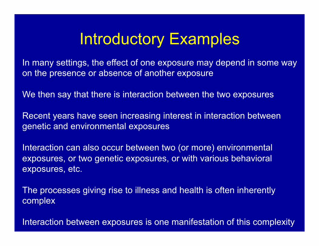
Introductory Examples In many settings, the effect of one exposure may depend in some way on the presence or absence of another exposure

We then say that there is interaction between the two exposures

Recent years have seen increasing interest in interaction between genetic and environmental exposures

Interaction can also occur between two (or more) environmental exposures, or two genetic exposures, or with various behavioral exposures, etc.

The processes giving rise to illness and health is often inherently complex

Interaction between exposures is one manifestation of this complexity

Introductory Examples Figueiredo et al. (2004) studied the effects of XRCC3-T241M polymorphisms and various environmental factors on breast cancer risk

For XRCC3-T241M using a case-control study they found the OR for breast cancer for the M/M genotype was 1.47 (CI: 1.00, 2.15) times that of the reference T/T or T/M genotype

However the effect varied by strata of alcohol consumption:

OR for Breast Cancer (by strata of alcohol consumption and XRCC3-T241M)

No Alcohol Alcohol T/T or T/M 1.00 1.12 (0.81-1.54) M/M 1.21 (0.70-2.09) 2.09 (1.16-3.78)

It seems as though XRCC3-T241M polymorphisms do not have much of an effect unless accompanied by alcohol consumption

This is an example of what we might call a gene-environment interaction

Introductory Examples In a review article, Hunter (2005) lists numerous examples of other “gene-environment interactions” including

Polymorphisms of: Environmental Exposure Outcome

MTHFR Folic acid Colorectal cancer NAT2 Heterocyclic amines in cooked meat Colorectal cancer APOE Dietary cholesterol Serum cholesterol ADH1C Alcohol intake MI PPARG2 Dietary fat Obesity

Likewise we might also be interested in the interactions of two genetic factors on various outcomes (though there are fewer clearer examples of this)

We will consider (i) statistical ideas to conceptualize interactions and (ii) how these relate to more mechanistic or causal notions of interaction

Notation We will let G denote our genetic factor of interest We will let E denote our environmental factor of interest We will let D denote our outcome of interest

For simplicity we will assume that G and E are binary i.e. E = 0 for the environmental exposure absent; E = 1 for present i.e. G = 0 for low genetic risk; G = 1 for high genetic risk

e.g. for a genetic factor with dominant mode of inheritance we let: G = 0 for a/a genotype G = 1 for a/A or A/A genotype (or for recessive inheritance G = 0 for a/a or a/A; G = 1 for A/A)

The ideas presented here apply more generally to exposures that are not binary

Additive Interactions How do we measure interaction? Suppose we had the following data on risks from a cohort study:

E=0 E=1 G=0 0.02 0.05 G=1 0.04 0.15

Let pij = P(D=1 | G=i, E=j ). A natural way to assess interactions is to measure the extent to which the effect of the two factors together exceeds the effect of each considered individually:

(p11 - p00) - [(p10 - p00) + (p01 - p00)] = p11 - p10 - p01 + p00

This is sometimes referred to as a measure of interaction on the additive scale

Additive Interactions Data: E=0 E=1 G=0 0.02 0.05 G=1 0.04 0.15

Additive measure of interaction: p11 - p10 - p01 + p00

If p11 - p10 - p01 + p00 > 0 the interaction is said to be positive or “super-additive” If p11 - p10 - p01 + p00 < 0 the interaction is said to be negative or “sub-additive”

Here we have: p11 - p10 - p01 + p00 = 0.15 - 0.04 - 0.05 + 0.02 = 0.08 > 0 i.e. a positive interaction

Multiplicative Interactions Data: E=0 E=1 G=0 0.02 0.05 G=1 0.04 0.15

As an alternative to assessing interactions on the additive scale using risks we might consider a multiplicative scale using relative risks:

Let RR11 = p11/p00 = 0.15/0.02 = 7.5 Let RR10 = p10/p00 = 0.04/0.02 = 2 Let RR01 = p01/p00 = 0.05/0.02 = 2.5

A measure of multiplicative interaction for risk ratios is: RR11 / (RR10 x RR01) = 7.5 / (2 x 2.5 ) = 7.5 / 5 = 1.5 If the multiplicative interaction is > 1 it is positive, < 1 it is negative

Multiplicative Interactions Data: E=0 E=1 G=0 0.02 0.05 G=1 0.04 0.15

In case control studies it is not in general possible to estimate risks or even risk ratios but one can still estimate odds ratios: Let OR11 = {p11/(1-p11)} / {p00/(1-p00)} Let OR10 = {p10/(1-p10)} / {p00/(1-p00)} Let OR01 = {p01/(1-p01)} / {p00/(1-p00)}

Interaction on the odds ratio scale is then measured by: OR11 / (OR10 x OR01) Again if this is > 1 the interaction is positive, if < 1 then negative If the outcome is rare then the OR interaction measure approximates the RR interaction measure

Additive vs. Multiplicative Interactions Conceived of in this way, interaction depends on the scale (multiplicative or additive)

We may in fact have additive interaction w/o multiplicative interaction E=0 E=1 G=0 0.02 0.05 G=1 0.04 0.10

Additive: p11 - p10 - p01 + p00 = 0.10 - 0.04 - 0.05 + 0.02 = 0.03 > 0

Multiplicative: RR11 / (RR10 x RR01) = 5 / (2 x 2.5) = 1

In other settings we may have multiplicative interaction but no additive interaction:

E=0 E=1 G=0 0.02 0.05 G=1 0.07 0.10

Additive: p11 - p10 - p01 + p00 = 0.10 - 0.07 - 0.05 + 0.02 = 0

Multiplicative: RR11 / (RR10 x RR01) = 5 / (3.5 x 2.5) = 0.57 < 1

Additive vs. Multiplicative Interactions

For some time in the epidemiologic literature, there was debate as to which scale one should assess interactions on (Blot and Day, 1979; Saracci, 1980; Rothman et al., 1980)

The general historical consensus was: (1) Often the additive scale is of greatest public health importance

It allows one to discern whether the effect would be different in different subgroups (Rothman et al., 1980)

(2) The additive scale also seemed to correspond to the more biological notion of synergism as conceived of by Rothman (1976); (later in lecture)

(3) However, sometimes the multiplicative scale (or neither scale) may be the one that more naturally corresponds to the biological mechanisms (Siemiatycki and Thomas, 1981); though in these cases the additive scale is still important for assessing public health impact


Suppose that E denotes some drug and the outcome is “cured”: And there are 100 with G=0 and 100 with G=1 and we have 100 doses E=0 E=1 G=0 0.01 0.05 G=1 0.04 0.10

The risk difference for E on those with G=0 is: 0.05 - 0.01 = 0.04 The risk difference for E on those with G=1 is: 0.10 - 0.04 = 0.06 p11 - p10 - p01 + p00 = 0.10 - 0.04 - 0.05 + 0.01 = 0.02 > 0

The risk ratio for E on those with G=0 is: 0.05 / 0.01 = 5 The risk ratio for E on those with G=1 is: 0.10 / 0.04 = 2.5 RR11 / (RR10 x RR01) = 10 / (5 x 4) = 0.5 < 1

If we give the drug to G=0 group we cure: 100*(0.05) + 100*(0.04) = 9 If we give the drug to G=1 group we cure: 100*(0.01) + 100*(0.10) = 11

We should treat the G=1 group; we cure an additional 2 persons Additive interaction (not multiplicative interaction) identifies this The risk ratio suggests treating the G=0 group; for public health purposes we should rely on additive interaction measure to decide which subgroups to target


In case-control studies we cannot in general estimate the risks themselves and generally odds ratios (which approximate risk ratios when the outcome is rare) are used. Assume a rare outcome so OR’s and RR’s are approximately equal: We cannot get the additive interaction directly but suppose we divide

Additive interaction p11 - p10 - p01 + p00 by p00 We get: RR11 - RR10 - RR01 + 1

This gives us something like the additive interaction but using RR’s (or OR’s); it is sometimes called the “Relative Excess Risk due to Interaction” or “RERI” (Rothman, 1986)

If RERI > 0 we have a positive additive interaction; if < 0 a negative additive interaction

We can thus assess additive interaction using risk ratios (or odds ratio if the outcome is rare)


Suppose we had a case-control study Assume the outcome is rare and we have the following OR’s or RR’s

E=0 E=1 G=0 1 2.5 G=1 2 5

Although we cannot get at the additive interaction directly we could estimate:

RR11 - RR10 - RR10 + 1 = 5 - 2 - 2.5 + 1 = 1.5 > 0

Although we have case-control data we know we still have positive interaction on the additive scale i.e. targeting one group will have greater public health benefit than targeting another group


In most published epidemiologic studies, interactions are evaluated and reported on the multiplicative scale

Interaction on the additive scale are often not e.g. perhaps only about 1 in 50 in epidemiology reported (Knol et al., 2009), even though there has been consensus that it should be reported for assessing public health relevance

The focus on multiplicative interaction is likely due to the statistical models which are used in such analyses (e.g. logistic regression) and the fact that the models employed immediately give interactions (and confidence intervals) on a multiplicative scale

In general, if interaction are interest it is probably good to report estimates and confidence intervals on both scales


Statistical Interactions

A statistical model on the linear scale accommodating interaction takes the form:

P(D=1|G=g,E=e) = α0 + α1g + α2e + α3eg

In the regression setting: α3 = p11 - p10 - p01 + p00 i.e. the interaction contrast on the additive scale

In fact: α0 = p00 α1 = p10 - p00 α2 = p01 - p00

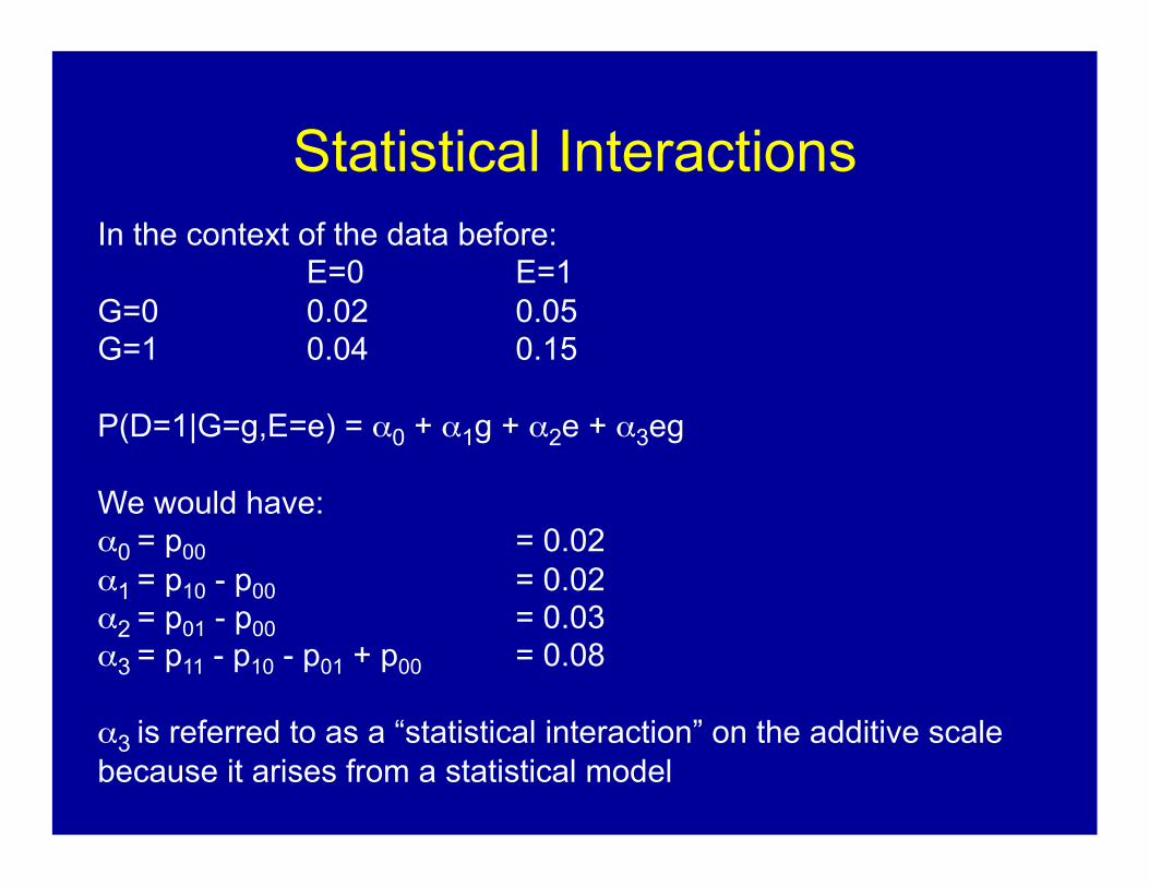
Statistical Interactions In the context of the data before: E=0 E=1 G=0 0.02 0.05 G=1 0.04 0.15

P(D=1|G=g,E=e) = α0 + α1g + α2e + α3eg

We would have: α0 = p00 = 0.02 α1 = p10 - p00 = 0.02 α2 = p01 - p00 = 0.03 α3 = p11 - p10 - p01 + p00 = 0.08

α3 is referred to as a “statistical interaction” on the additive scale because it arises from a statistical model

Statistical Interactions Similarly one might have a “log-linear” model for risk ratios: log {P(D=1|G=g,E=e)} = β0 + β1g + β2e + β3eg

exp(β0) = p00 exp(β1)= RR10 exp(β2) = RR01 exp(β3) = RR11 / (RR10 x RR01)

Or one might alternatively use a “logistic” model for odds ratios: logit {P(D=1|G=g,E=e)} = β0 + β1g + β2e + β3eg

exp(β0)=p00/(1-p00) (cohort study only) exp(β1)=OR10 exp(β2) = OR01 exp(β3) = OR11 / (OR10 x OR01)

In these cases β3 is again referred to as a “statistical interaction” but now on the risk ratio or odds ratio scale

Logistic Regression and the Delta Method

For RERI, if the outcome is rare (so that odds ratios approximate risk ratios; or if incidence density sampling is used) we can calculate RERI using the coefficients of a logistic regression model:

logit {P(D=1|G=g,E=e)} = β0 + β1g + β2e + β3eg

We can then calculate:

RERI ≈ OR11 - OR10 - OR01 + 1 = exp(β1 + β2 + β3) - exp(β1) - exp(β2) + 1

Statistical Interactions Consider again the data from Figueiredo et al. (2004) with odds ratios compared to the reference category G=0 (i.e. T/T or T/M) and E=0 (i.e. no alcohol):



exp(β1) = 1.21 exp(β2) = 1.12 exp(β3) = OR11 / (OR10 x OR01) = 2.09 / (1.21 x 1.12) = 1.54 There is a positive interaction on the multiplicative scale

Also RERI ≈ OR11 - OR10 - OR01 + 1 = 2.09 - 1.21 - 1.12 + 1.00 = 0.76 > 0 There is a positive interaction on the additive scale as well

Statistical Interactions The software used to fit models such as:

P(D=1|G=g,E=e) = α0 + α1g + α2e + α3eg logit {P(D=1|G=g,E=e)} = β0 + β1g + β2e + β3eg

will give confidence intervals and p-values for the interaction coefficients, i.e. α3 and β3 respectively.

These statistical models can also easily accommodate additional confounding variables or covariates in the model

For RERI, Hosmer and Lemeshow (1992) give standard errors using the delta method Lundberg et al. (1996) provides some SAS code to do these computations automatically Knol and VanderWeele (2012) provide an easy-to-use Excel spreadsheet to do this

Case-Only Estimators One other more recent approach deserves attention Consider the interaction term β3 in a logistic regression


Suppose also that G is independent of E in the population (plausible in many gene-environment interaction studies) and that the outcome is rare

Suppose that data are only collected on the cases (D=1) It turns out that the odds ratio relating G and E among the cases is equal to the interaction measure on the multiplicative scale exp(β3) (Yang et al. 1999; cf. Piergorsch et al., 1994)

P(G=1|E=1,D=1)/(P(G=0|E=1,D=1) = exp(β3) = RR11/(RR10 x RR01) P(G=1|E=0,D=1)/(P(G=0|E=0,D=1)

Essentially to get measures of multiplicative interaction, all that is needed is data on G and E among the cases

Case-Only Estimators This is referred to as the “case-only” estimator of interaction The case-only estimator depends critically on the assumption of GxE independence and can be quite biased if this is violated (Albert et al., 2001)

Under this assumption of GxE independence the case-only estimator is in fact more efficient than using the standard estimate from a logistic regression

We can condition on covariates C to make independence more plausible With the case-only estimator we can estimate the interaction parameter β3

logit {P(D=1|G=g,E=e,C=c)} = β0 + β1g + β2e + β3eg + β4’c

but we cannot estimate the main effect of the logistic regression

Estimates and confidence intervals for the case-only estimator can be obtained by running a logistic regression of G on E and C among the cases: logit {P(G=1|E=e,C=c,D=1)} = θ0 + β3e + θ1’c

Mechanistic Interactions…?

Do statistical interactions tell us anything about biological or mechanistic interactions?

Several authors have pointed out the potential danger of using statistical interaction to draw conclusions about biological interaction (Siemiatycki and Thomas, 1981; Thomas, 1991; Rothman and Greenland, 1998; Cordell, 2002)

How might we conceive of mechanistic interaction?

Can we conclude anything about mechanistic interaction from statistical interaction…?

Mechanistic Interaction

Sufficient Causation in Statistics and Epidemiology

Rothman (1976) defined a “sufficient cause” as minimal set of events, conditions or characteristics that inevitably produced the disease; a “component cause” (or “cause”) was an individual event, condition or characteristic required by a given sufficient cause.

G3 G2

E1 • Rothman also provided a schematic for these component causes which have come to be known as “causal pies” • There has been some work relating sufficient component causes to potential outcomes (Greenland and Poole 1988, Rothman and Greenland 1998, Aickin 2002, Flanders 2006, VanderWeele and Hernan 2006, VanderWeele and Robins 2007, 2008) • Similar ideas also appeared earlier in the philosophical literature (Mackie, 1965)

We may want to know whether two causes G and E are ever both present in the same sufficient cause

E

G

???

D

Mechanistic Interaction

Negative multiplicative interaction with no mechanistic interaction

A1G

A0

A2E

D

There is no mechanism requiring both G and E

There is no interaction between G and E in a mechanistic sense

Suppose there are just three mechanisms for outcome D One requiring G and some other factors A1

One requiring E and some other factors A2

One requiring neither G nor E, just some other factors A0

Suppose that G and E are independent in the population

Negative multiplicative interaction with no mechanistic interaction

G E Total Cases RR G=0 E=0 3980 20 1 G=1 E=0 980 20 4.0 G=0 E=1 3920 80 4.0 G=1 E=1 965 35 7.0

Multiplicative interaction: RR11 / (RR10 x RR01) =7.0/(4 x 4) = 0.44 < 1

RERI = 7.0 - 4.0 - 4.0 + 1 = 0

We have a non-zero negative multiplicative interaction but… This can arise without any sort of mechanistic interaction! i.e. no mechanism with both G and E

Suppose G, E, A1, A2 and A0 are all independent in the population Suppose G and E occur with probabilities 0.2 and 0.5 respectively Suppose A1 and A2 each occur with probability 0.015 Suppose A0 occurs with probability 0.005 Suppose there are 10,000 subjects in the population

Positive multiplicative interaction with no mechanistic interaction

There is no mechanism requiring both G and E

There is no interaction between G and E in a mechanistic sense

A1G

A3G

A2E

D

Suppose there are three mechanisms for outcome D One requiring G and some other factors A1

One requiring E and some other factors A2

One requiring absence of G (denoted by G) and factors A3

Suppose that G and E are independent in the population

Positive multiplicative interaction with no mechanistic interaction

Suppose G and E are independent and occur with probabilities 0.4 and 0.5 respectively Suppose distribution of A1, A2 and A3 is as follows P(A1 =0, A2 =1, A3 =1) = .004 P(A1 =1, A2 =0, A3 =0) = .004 P(A1 =0, A2 =1, A3 =0) = .001 P(A1 =1, A2 =1, A3 =0) = .001 P(A1 =0, A2 =0, A3 =0) = .99 Suppose there were 10,000 subjects in the population

G E Total Cases RR G=0 E=0 3000 12 1 G=1 E=0 2000 10 1.25 G=0 E=1 3000 18 1.50 G=1 E=1 2000 20 2.50

RR11 / (RR10 x RR01) = 2.50 / (1.25 x 1.50) = 1.33 > 1

RERI = 2.50 - 1.50 - 1.25 + 1 = 0.75 > 0

We have positive multiplicative and additive interaction

But there is no mechanistic interaction

Notation and Definitions When can we conclude that there is a mechanism that requires both exposures?

Counterfactuals: Let Dge denote the counterfactual outcome for an individual if, possibly contrary to fact, G is set to g and E is set to e

Causal Interaction: We say that there is causal interaction (or “sufficient cause interaction”) if for some individual D11=1 but D10=D01=0

It can be shown that if such “causal interaction” is present then there must be “synergism” in Rothman’s sufficient cause framework (VanderWeele and Robins, 2008) i.e. a sufficient cause with both G and E

Mechanistic Interaction We might ask…

Are there individuals who would develop breast cancer with the XRCC3-T241M risk allele and alcohol consumption but not if only one or the other were present?

Are there individuals who would have diarrheal disease if infected with both E. coli/Shigella and rotavirus but not if just infected with one or the other?

Are there individuals who would develop esophageal cancer only if both of two genetic variants are present?

These are questions about mechanistic interaction, not statistical interaction

Mechanistic Interaction Such sufficient cause interaction is not equivalent to statistical interaction (Greenland and Poole, 1988; Rothman and Greenland, 1998)

Testing for such sufficient cause interaction in general requires stronger assumptions than statistical interaction

Monotonicity: We will then say that G has a positive “monotonic effect” on the outcome D if Dge is non-decreasing in g (similarly for E)

Monotonicity requires the effect always operates in the same direction for all individuals; it might be plausible sometimes (e.g. the effect of smoking on lung cancer) but not others (e.g. alcohol on stroke)

Unconfoundedness: We say that the effects of G and E on D are unconfounded if P(Dge=1)=P(D=1|G=g,E=e)

Mechanistic Interaction Let pge = P(D=1|G=g,E=e)

Rothman and Greenland (1998) show that if the effects of G and E on D are unconfounded and if both G and E have positive monotonic effects on the outcome then one can test for a sufficient cause interaction by testing: p11 - p10 - p01 + p00 > 0 i.e. positive additive interaction [the effects of both exposures combined exceed the sum of the effects of each considered separately] We could also test this by RERI > 0

Rothman and Greenland (1998) go on to claim that without monotonicity conclusions about sufficient cause interaction cannot be drawn empirically with data

Mechanistic Interaction Result (VanderWeele and Robins, 2007, 2008): If the effects of G1 and G2 on D are unconfounded one can test for a sufficient cause interaction by testing: p11 - p10 - p01 > 0

This condition can be expressed as RERI > 1 It is a stronger condition than simply having positive additive interaction which would only require RERI > 0

By using this stronger condition one can in fact test for sufficient cause interaction even without monotonicity, contrary to what was previously thought

In the 3rd Edition of Modern Epidemiology, Rothman et al. (2008) correct the claim and discuss these results

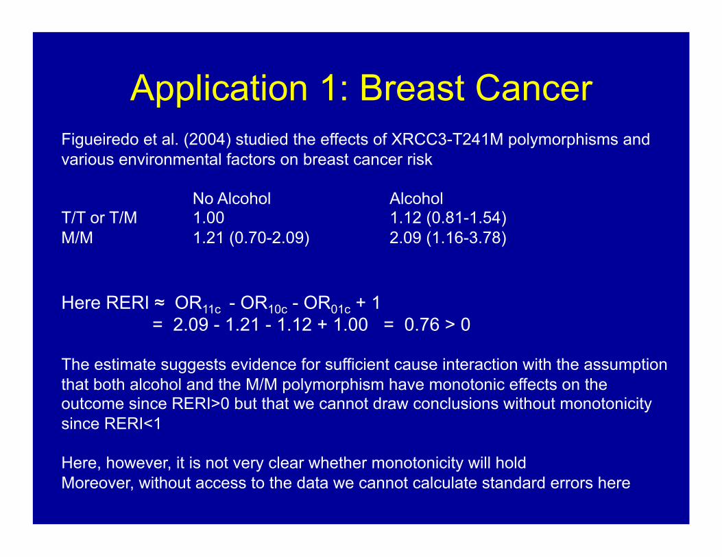
Application 1: Breast Cancer Figueiredo et al. (2004) studied the effects of XRCC3-T241M polymorphisms and various environmental factors on breast cancer risk


Here RERI ≈ OR11c - OR10c - OR01c + 1 = 2.09 - 1.21 - 1.12 + 1.00 = 0.76 > 0

The estimate suggests evidence for sufficient cause interaction with the assumption that both alcohol and the M/M polymorphism have monotonic effects on the outcome since RERI>0 but that we cannot draw conclusions without monotonicity since RERI<1

Here, however, it is not very clear whether monotonicity will hold Moreover, without access to the data we cannot calculate standard errors here

Application 2: Diarrheal Disease Data from a case-control study in Northwestern Ecuador (2003-2008) indicates that (Bhavnani et al., 2012): Giardia rotavirus E. coli/Shigella are all associated with increased risk of diarrheal disease

There is also strong evidence of interaction:

Giardia & rotavirus: RERI=10.7-2.6-1.1+1 = 7.9 (95% CI: 3.1, 18.9) E. coli/Shigella & rotavirus: RERI=13.2-2.6-1.6+1 = 9.9 (95% CI: 2.6, 28.4) E. coli/Shigella & giardia: RERI= 3.0-1.1-1.6+1 = 1.2 (95% CI: -1.4, 3.1)

For Giardia & rotavirus and for E. coli/Shigella & rotavirus, there is strong evidence of mechanistic interaction even without making any monotoncity assumptions (VanderWeele, 2012)

Epistasis Somewhat related ideas and issues appear in the genetics literature

Often the term “epistasis” is used to describe statistical interaction between two genetic factors

Cordell (2002, 2009) points out that although the word “epistasis” is now essentially used simply to describe a statistical gene-gene interaction, the word originally had a somewhat different sense

Bateson (1909) used “epistasis” to describe instances in which the effect of a particular genetic variant was masked by a variant at another locus so that variation of phenotype with genotype at one locus was only apparent amongst those with certain genotypes at the second locus

Epistasis Suppose then we think of interaction this way (different from the statistical approach) and ask the question whether there are any individuals for whom the first genetic factor G1 has no effect on the outcome unless the second genetic factor G2 is present (e.g. G2=1) as in the Table below:

G2=0 G2=1 G1=0 0 0 G1=1 0 1

We would then say that G1 is epistatic to G2 (the effect G1 can be masked if G2=0)

In our counterfactual notation, this would be: D11=1 but D10=D01=D00=0

Although this is a conceptually distinct notion from that of a statistical interaction, current terminology does not distinguish between “statistical gene-gene interaction” and “epistasis” in the sense of Bateson (1909)

Epistasis Cordell (2009) notes that Fisher (1933) used the term “epistacy” for statistical gene-gene interaction, distinguishing it from Bateson’s “epistasis”

However, the two terms were very similar and with time “epistasis” came to be used synonymously with “statistical interaction” between genetic factors

With the greater recognition that the two are distinct concepts, Phillips (2008) proposed using “statistical epistasis” for statistical interaction between two genetic factors and “compositional epistasis” for epistasis in the sense of masking (and “functional epistasis” for physical interaction)

The terminology has been adopted by others (Cordell, 2009; Moore & Williams, 2009)

Compositional epistasis: We say that there is compositional epistasis if for some individual D11=1 but D10=D01=D00=0 (This is stronger than a sufficient cause interaction)

Epistasis

Cordell (2002, 2009) moreover pointed out that tests for statistical interactions (“statistical epistasis”) will generally be of limited use in drawing conclusions about epitasis in the sense of masking (“compositional epistasis”) as Bateson had originally conceived of it

Although tests for ordinary statistical interaction between two genetic factors do not in general allow one to draw conclusions about epistasis, progress can be made for empirically testing for compositional epistasis

There are relations between empirical data patterns and compositional epistasis that have not been previously noted and that can be used to derive non-standard interaction tests to empirically test for such compositional epistasis (VanderWeele, 2010)

Epistasis Result (VanderWeele, 2010): If the effects of G1 and G2 on D are unconfounded then “compositional epistasis” is present if: p11 - p10 - p01 - p00 > 0

If at least one of the effects of G1 and G2 are monotonic then: p11 - p10 - p01 > 0 suffices

If the effects of both G1 and G2 are monotonic then: p11 - p10 - p01 + p00 > 0 suffices.

Only the final condition (under monotonicity) is the same as an additive interaction But we can test for compositional epistasis without monotonicity, using the other stronger empirical conditions Results were reported in Nature Reviews Genetics (VanderWeele, 2010)

Epistasis The measure RERI can also be used for testing for compositional epistasis RERI = OR11 - OR10 - OR01 + 1 ≈ RR11 - RR10 - RR01 + 1

The results above imply that to test for compositional epistasis: If both G1 and G2 have monotonic effects then we can test: RERI > 0 If only one of the factors has a monotonic effect we can test: RERI > 1 Without any monotonicity assumptions we can test: RERI > 2

The empirical conditions have analogues for multiplicative models Suppose the outcome is rare and we use a logistic model: logit {P(D=1|G1=g1,G2=g2)} = β0 + β1g1 + β2g2 + β3g1g2

If main effects β1 and β2 are non-negative the following conditions suffice: If both G1 and G2 have monotonic effects then we can test: β3 > 0 If only one of the factors has a monotonic effect we can test: β3 > log(2) Without any monotonicity assumptions we can test: β3 > log(3)

Application 3: Esophageal Cancer Yang et al. (2005) examine interaction in the effects of Arg variants on ADH2

(chr 4) and Glu/Glu versus Glu/Lys on ALDH2 (chr 12) on esophageal cancer

Using the case-control data from Yang et al. (2005) to examine additive interaction using the relative excess risk due to interaction one finds:

RERI = OR11 - OR10 - OR01 + 1 = 7.20 - 1.40 - 3.52 + 1 = 3.28 (95% CI: 0.4, 6.16)

The estimate RERI = 3.28 > 2 would suggest compositional epistasis without any assumptions about monotonicity at all

The confidence interval contains a value as small as RERI = 0.4 > 0 which would imply compositional epistasis only if both variants had monotonic effects on esophageal cancer

In a recent review article on gene-gene interaction (“epistasis”) Phillips (2008) distinguished three types of epistasis:

(1) Statistical epistasis (i.e. interaction in a statistical model) (2) Compositional epistasis (e.g. D occurs if and only if G1=G2=1) (3) Functional epistasis (e.g. the physical interaction of proteins)

We have considered new tests for “compositional epistasis” It was previously thought that such epistasis could not be detected

using statistical tests (Cordell, 2002); one can test for it but this requires non-standard interaction test (VanderWeele 2010ab)

But even compositional epistasis does not necessarily imply functional epistasis, i.e. the physical interaction of proteins

Further Remarks

Suppose that G1 and G2 are two genetic factors Suppose that when G1=1 protein 1 is not produced Suppose that when G2=1 protein 2 is not produced

Suppose that the outcome D occurs if and only if neither protein 1 nor protein 2 are present

We then have an epistatic interaction: the outcome occurs if and only if G1=1 and G2=1

But we do not have physical interaction here It is precisely the absence of the proteins that gives rise to the outcome (there is nothing to physically interact here)

It is important to understand the limits of the conclusions being drawn about these alternative forms of causal interaction

Further Remarks

Sufficient cause interaction was sometimes earlier referred to as “biologic interaction” (e.g. Rothman and Greenland, 1998); and sometimes just additive interaction was even referred to as “biologic interaction” (Andersson et al., 2005)

As we have seen, neither statistical interaction nor even sufficient cause interaction necessarily tells us anything about physical or functional interactions

Statistical analyses can only tell us limited information about the underlying biology (Siemiatycki and Thomas, 1981; Thomas, 1991; Rothman and Greenland, 1998; Cordell, 2002)

Because of this there has been a suggestion to move away from the use “biologic interaction” for sufficient cause interactions (cf. Lawlor, 2011; VanderWeele, 2011)

It may be more appropriate to refer to these sufficient cause or epistatic interactions as “mechanistic interactions” (both exposures together turns the outcome ‘on’ and the removal of one turns the outcome ‘off’)

Further Remarks

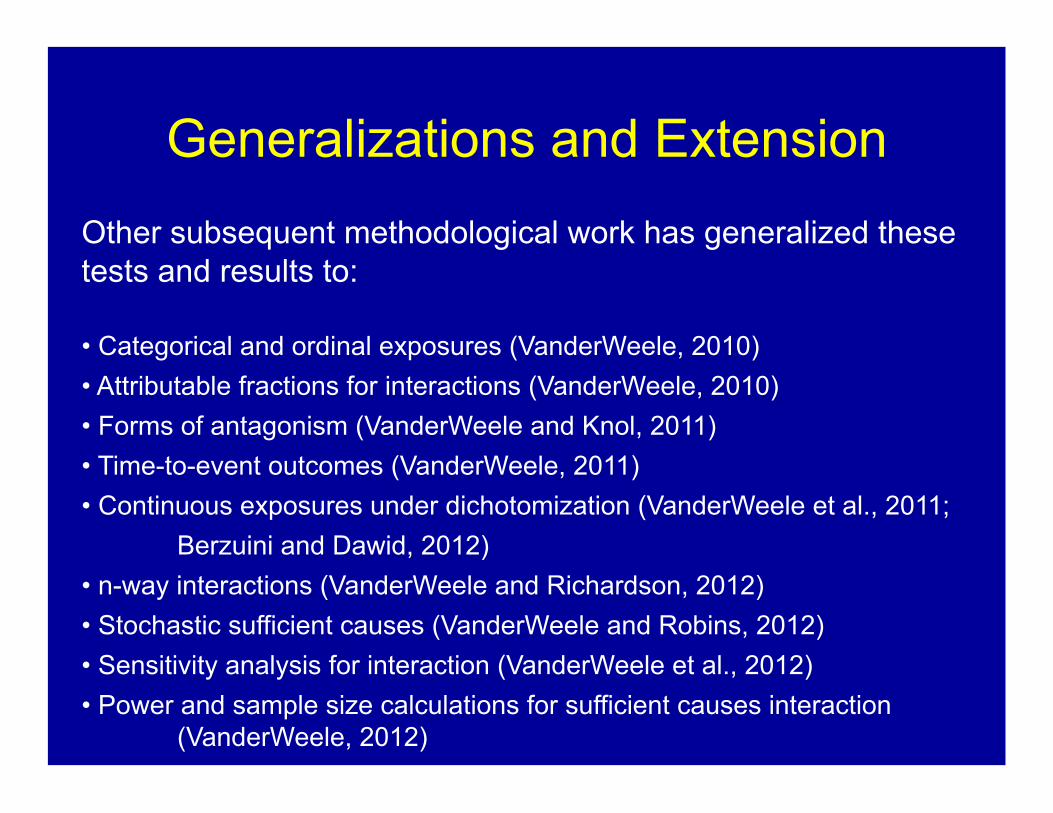
Generalizations and Extension Other subsequent methodological work has generalized these tests and results to:

• Categorical and ordinal exposures (VanderWeele, 2010) • Attributable fractions for interactions (VanderWeele, 2010) • Forms of antagonism (VanderWeele and Knol, 2011) • Time-to-event outcomes (VanderWeele, 2011) • Continuous exposures under dichotomization (VanderWeele et al., 2011; Berzuini and Dawid, 2012) • n-way interactions (VanderWeele and Richardson, 2012) • Stochastic sufficient causes (VanderWeele and Robins, 2012) • Sensitivity analysis for interaction (VanderWeele et al., 2012) • Power and sample size calculations for sufficient causes interaction (VanderWeele, 2012)

Application 4: Skin Lesions High levels of arsenic has been found in well water in Bangladesh HEALS study was design to assess long-term health consequences of arsenic and move participants to safer wells Data from large cohort study in Bangladesh (about 10,000 individuals)

Let X1 for level of arsenic in well water (µg/L), a continuous exposure Let X2=1 for smoking (ever vs. never) Let D denote our outcome, pre-malignant skin lesions

Covariate control for: sex, age, education, BMI, land and TV ownership (markers of socioeconomic status in Bangladesh), fertilizer use and pesticide use

Using methods for continuous exposures, there is evidence for mechanistic interaction between smoking and arsenic in well water for arsenic levels above about 80 µg/L

Application 4: Skin Lesions Plot of magnitude of additive interaction by level of well-water arsenic

There is strong evidence for causal interaction around values >80 µg/L

Concluding Remarks (1) Assessing interaction can be important when it is thought that the effect

of one exposure depends on another

(2) When interaction is of interest, both additive and multiplicative interaction can and should be reported

Additive interaction is always relevant for public health purposes

(3) Mechanistic forms of interaction (sufficient cause and epistatic interaction) are distinct from statistical interaction

(4) One can empirically test for these with data; the conditions are closely related to additive interaction

However in each case, without further assumptions about monotonicity the conditions for these causal interactions are stronger than simply statistical interactions

(5) It is important to understand the limits of the conclusions being drawn about these alternative forms of causal interaction

References Part I Blot WJ, Day NE. Synergism and interaction: are they equivalent? Am. J. Epidemiol. 1979;110:99-100.

Figueiredo JC, Knight JA, Briollais L, Andrulis IL, Ozcelik H. (2004). Polymorphisms XRCC1-R399Q and XRCC3-T241M and the risk of breast cancer at the Ontario Site of the Breast Cancer Family Registry. Cancer Epidemiology, Biomarkers and Prevention 13:583-591.

Hosmer, D.W., Lemeshow, S. (1992). Confidence interval estimation of interaction. Epidemiology 3:452-56.

Knol MJ, Egger M, Scott P, Geerlings MI, Vandenbroucke JP. When One Depends on the Other: Reporting of Interaction in Case-Control and Cohort Studies. Epidemiology. 2009; 20:161-166.

Knol, M.J. and VanderWeele, T.J. (2012). Guidelines for presenting analyses of effect modification and interaction. International Journal of Epidemiology, 41:514-520.

Hunter DJ. (2005). Gene-environment interactions in human diseases. Nature Reviews Genetics, 6:287-298.

References

Lundberg, M., Fredlund, P., Hallqvist, J., Diderichsen, F. (1996). A SAS program calculating three measures of interaction with confidence intervals. Epidemiology 7:655-656.

Rothman KJ. (1976). Causes. Am J of Epidemiol 104:587-592.

Rothman, K. J. Modern Epidemiology. 1st ed. Little, Brown and Company, Boston, MA (1986).

Rothman KJ, Greenland S. Modern Epidemiology. Philadelphia: Lippincott-Raven, 1998.

Rothman KJ, Greenland S, Walker AM. Concepts of interaction. Am. J. Epidemiol. 1980;112:467-470.

Saracci R. Interaction and synergism. Am. J. Epidemiol. 1980;112:465-466.

References Siemiatycki J, Thomas DC (1981). Biological models and statistical interactions: an example from multistage carcinogenesis. Int. J. Epidemiol. 10:383-387.

VanderWeele, T.J. (2009). On the distinction between interaction and effect modification. Epidemiology, 20:863-871.

VanderWeele, T.J. and Knol, M.J. (2011). The interpretation of subgroup analyses in randomized trials: heterogeneity versus secondary interventions. Annals of Internal Medicine, 154:680-683.

VanderWeele TJ, Robins JM. (2007) The identification of synergism in the SCC framework. Epidemiol, 18:329-339.

VanderWeele, T.J. and Robins, J.M. (2007). Four types of effect modification – a classification based on directed acyclic graphs. Epidemiology 18:561-568.

References Part II Andersson, T., Alfredsson, L., Kallberg, H., Zdravkovic, S. and Ahlbom, A. (2005). Calculating measures of biological interaction. European Journal of Epidemiology 20:575-579.

Cordell, H.J. (2002) Epistasis: what it means, what it doesn’t mean, and statistical methods to detect it in humans. Human Molecular Genetics, 11:2463-2468. Cordell, H.J. (2009). Detecting gene-gene interaction that underlie human diseases. Nature Reviews Genetics, 10:392-404.

Greenland, S. and Poole, C. (1988). Invariants and noninvariants in the concept of interdependent effects. Scandinavian Journal of Work, Environment and Health, 14:125-129. Lawlor, D.A. (2011). Biological interaction: time to drop the term? Epidemiology, 22:148-50.

Phillips, P.C. (2008). Epistasis – the essential role of gene interactions in the structure and evolution of genetic systems. Nature Reviews Genetic, 9:855-867. Rothman, K.J. (1976). Causes. American Journal of Epidemiology, 104:587-592.

References Stern MC, Johnson LR, Bell DA, Taylor JA. XPD codon 751 polymorphism, metabolism genes, smoking, and bladder cancer risk. Cancer Epidemiology, Biomarkers and Prevention 2002; 11:1004-1011.

Stern MC, Umbach DM, Lunn RM, Taylor JA. DNA repair gene XCRR3 codon 241 polymorphism, its interaction with smoking and XRCC1 polymorphisms, and bladder cancer risk. Cancer Epidemiology, Biomarkers and Prevention 2002; 11:939-943.

Thomas, W. (1991) Effect modification and the limits of biological inference from epidemiologic data. Journal of Clinical Epidemiology, 44:221-232.

VanderWeele, T.J. (2009). Sufficient cause interactions and statistical interactions. Epidemiology, 20:6-13. VanderWeele, T.J. (2010). Empirical tests for compositional epistasis. Nature Reviews Genetics, 11:166. VanderWeele, T.J. (2010). Empirical tests for compositional epistasis. Nature Reviews Genetics, 11:166.

References

VanderWeele, T.J. (2010). Epistatic interactions. Statistical Applications in Genetics and Molecular Biology, 9, Article 1:1-22.

VanderWeele, T.J. (2011). A word and that to which it once referred: assessing "biologic" interaction. Epidemiology, 22:612-613.

VanderWeele, T.J., Hernández-Diaz, S. and Hernán, M.A. (2010). Case-only gene-environment interaction studies: when does association imply mechanistic interaction? Genetic Epidemiology, 34:327-334

VanderWeele, T.J. and Knol, M.J. (2011). Remarks on antagonism. American Journal of Epidemiology, 173:1140-1147. VanderWeele, T.J. and Robins J.M. (2007), The identification of synergism in the sufficient-component cause framework. Epidemiology, 18:329-339. VanderWeele, T.J. and Robins, J.M. (2008). Empirical and counterfactual conditions for sufficient cause interactions. Biometrika, 95:49-61.

References

VanderWeele, T.J., Vansteelandt, S. and Robins, J.M. (2010). Marginal structural models for sufficient cause interactions. American Journal of Epidemiology, 171:506-514.

Vansteelandt, S., VanderWeele, T.J., Tchetgen, E.J., Robins, J.M., (2008). Multiply robust inference for statistical interactions. Journal of the American Statistical Association, 103:1693-1704.

Vansteelandt, S., VanderWeele, T.J. and Robins, J.M., Semiparametric inference for sufficient cause interactions. Journal of the Royal Statistical Society, Series B, in press.

Xu WH, Dai Q, Xiang YB, Long JR, Ruan ZX, Cheng JR, Zheng W, Shu XO. Interaction of soy food and tea consumption with CYP19A1 Genetic polymorphisms in the development of endometrial cancer. American Journal of Epidemiology 2007;166:1420-1430.

Documents

An Introduction to Interaction Analysis - Harvard … Introduction to Interaction Analysis Tyler J. VanderWeele Departments of Epidemiology and Biostatistics Harvard School of Public