Embed Size (px)
Citation preview

An Introduction to Hybrid Automata,Numerical Simulation andReachability Analysis
Goran FrehseSyDe Summer School, September 10, 2015Univ. Grenoble Alpes – Verimag,2 avenue de Vignate, Centre Equation,38610 Gières, France,[email protected]
Overview
Hybrid Automata
Numerical Simulation
Set-Based Reachability
Conclusions
2
Overview
Hybrid Automata
Running Example
Definition and Semantics
Numerical Simulation
Set-Based Reachability
Conclusions
3

Running Example: Ball on String
mFs
Fg
xr
xr + L
x
(a) extension
m
Fgxr
xr + L
x
(b) freefall
4
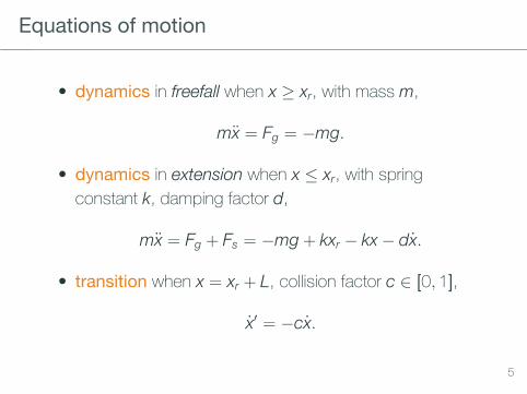
Equations of motion
• dynamics in freefall when x ≥ xr, with mass m,
mx = Fg = −mg.
• dynamics in extension when x ≤ xr, with springconstant k, damping factor d,
mx = Fg + Fs = −mg + kxr − kx− dx.
• transition when x = xr + L, collision factor c ∈ [0, 1],
x′ = −cx.
5
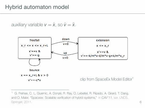
Hybrid automaton model
auxiliary variable v = x, so v = x.
clip from SpaceEx Model Editor1
1 G. Frehse, C. L. Guernic, A. Donzé, R. Ray, O. Lebeltel, R. Ripado, A. Girard, T. Dang,and O. Maler, “Spaceex: Scalable verification of hybrid systems,” in CAV’11, ser. LNCS,Springer, 2011. 6

Behavior
0 0.5 1 1.5 2 2.5−1
0
1
x0
x1
x2
x3 x4
x5
t
posit
ionx
0 0.5 1 1.5 2 2.5
−5
0
5
v0
v1
v−2
v2
v3
v4
v5
t
veloc
ityv
7
Overview
Hybrid Automata
Running Example
Definition and Semantics
Numerical Simulation
Set-Based Reachability
Conclusions
8
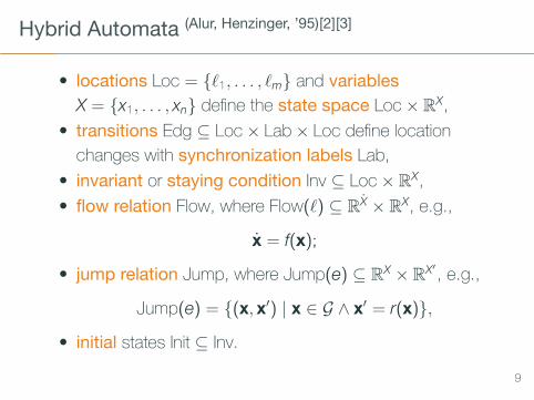
Hybrid Automata (Alur, Henzinger, ’95)[2][3]
• locations Loc = ℓ1, . . . , ℓm and variablesX = x1, . . . , xn define the state space Loc× RX,
• transitions Edg ⊆ Loc× Lab× Loc define locationchanges with synchronization labels Lab,
• invariant or staying condition Inv ⊆ Loc× RX,• flow relation Flow, where Flow(ℓ) ⊆ RX × RX, e.g.,
x = f(x);
• jump relation Jump, where Jump(e) ⊆ RX × RX′ , e.g.,
Jump(e) = (x, x′) | x ∈ G ∧ x′ = r(x),
• initial states Init ⊆ Inv.
9
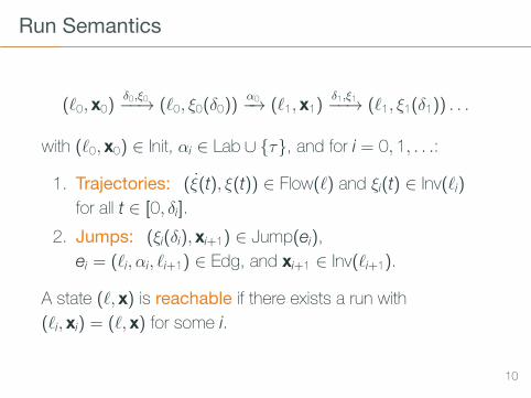
Run Semantics
(ℓ0, x0)δ0,ξ0−−→ (ℓ0, ξ0(δ0))
α0−→ (ℓ1, x1)δ1,ξ1−−→ (ℓ1, ξ1(δ1)) . . .
with (ℓ0, x0) ∈ Init, αi ∈ Lab ∪ τ, and for i = 0, 1, . . .:
1. Trajectories: (ξ(t), ξ(t)) ∈ Flow(ℓ) and ξi(t) ∈ Inv(ℓi)
for all t ∈ [0, δi].2. Jumps: (ξi(δi), xi+1) ∈ Jump(ei),
ei = (ℓi, αi, ℓi+1) ∈ Edg, and xi+1 ∈ Inv(ℓi+1).
A state (ℓ, x) is reachable if there exists a run with(ℓi, xi) = (ℓ, x) for some i.
10
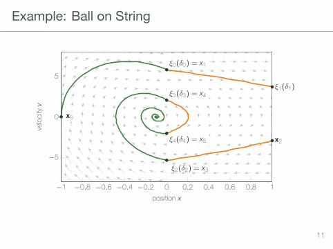
Example: Ball on String
−1 −0.8 −0.6 −0.4 −0.2 0 0.2 0.4 0.6 0.8 1
−5
0
5
x0
ξ0(δ0) = x1
ξ3(δ3) = x4ξ1(δ1)
x2
ξ2(δ2) = x3
ξ4(δ4) = x5
position x
veloc
ityv
11

Overview
Hybrid Automata
Numerical Simulation
Solving ODEs
Computing Trajectories and Jumps
Set-Based Reachability
Conclusions
12

Solving ODEs
Given an ordinary differential equation (ODE)
x = f(x), with initial value x0,
find ξ(t) with ξ(0) = x0 and ξ(t) = f(ξ(t)) for all t ≥ 0.
Numerical solution by computing x0, . . . , xN such thatxi ≈ ξ(ti) at time points t0, . . . , tN.2
Using fixed time step h: ti = ih.
2 R. P. Canale and S. C. Chapra, “Numerical methods for engineers,” Mc Graw Hill, NewYork, 1998. 13

Euler’s Method
Compute x0, . . . , xN with the sequence
xi+1 = xi + f(xi)h.
Comparing to Taylor series around xi,
xi+1 = xi + xih +xi2!h
2 + . . .+
(n−1)xin! hn + · · · ,
obtain estimate of local error εa = O(h2).
• global error εg = O(h)⇒ first-order method• accuracy limited by numerical roundoff error O(1/h)
14
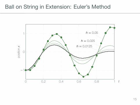
Ball on String in Extension: Euler’s Method
0 0.2 0.4 0.6 0.8 1
−1
0
1 h = 0.05
h = 0.025h = 0.0125
t
posit
ionx
15

Ball on String in Extension: Euler’s Method
x1
x2
x3
h = 0.05h = 0.025
−1.5 −1 −0.5 0 0.5 1 1.5
−10
−5
0
5
10
15
x0
x
veloc
ityv
16

Stability
The linear ODEx = ax,
converges to zero iff a < 0.
Euler’s method
xi+1 = xi + f(xi)h = xi + axih = (1 + ah)xi
converges to zero iff |1 + ah| < 1⇒ conditionally stable.
17
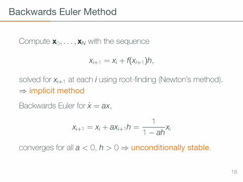
Backwards Euler Method
Compute x0, . . . , xN with the sequence
xi+1 = xi + f(xi+1)h,
solved for xi+1 at each i using root-finding (Newton’s method).⇒ implicit method
Backwards Euler for x = ax,
xi+1 = xi + axi+1h =1
1− ahxi
converges for all a < 0, h > 0⇒ unconditionally stable.
18
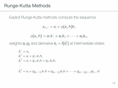
Runge-Kutta Methods
Explicit Runge-Kutta methods compute the sequence
xi+1 = xi + ϕ(xi, h)h,
ϕ(xi, h) = a1k1 + a2k2 + · · ·+ ankn,
weights ai,qij and derivative kj = f(xij) at intermediate states
xi1= xi,
xi2= xi + q11k1h,
xi3= xi + q21k1h + q21k2h,
...xi
n= xi + q(n−1)1k1h + q(n−1)2k2h + · · ·+ q(n−1)(n−1)kn−1h
19

Runge-Kutta Methods (Kutta, 1901)
Runge-Kutta method defined by n and parameters ai,qij
chosen to match first n terms of Taylor series.
Remaining degrees of freedom used to optimize, e.g.,truncation error O(hn+1) and global error O(hn) forn = 2, . . . , 5.
Ralston’s method has the smallest truncation error for n = 2:
k1 = f(x1i ), x1
i = xi,
k2 = f(x2i ), x2
i = xi + 3/4k1h,ϕ(xi, h) = 1
3k1 +23k2.
20
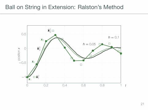
Ball on String in Extension: Ralston’s Method
0 0.2 0.4 0.6 0.8 1
−1
−0.5
0
0.5h = 0.1
x1
x2
x3
x21
x22
x23
h = 0.05
t
posit
ionx
21

Ball on String in Extension: Ralston’s Method
x21
x22
x23
x24
h = 0.1
x1
x2
x3
x4
h = 0.05
−1 −0.5 0 0.5
−5
0
5
x0
x
veloc
ityv
22

Error Estimation
Error estimation using difference between
• results for time steps h/2 and h,• results for (n− 1)th and nth order solver.
Runge-Kutta-Fehlberg (RKF) methods (Fehlberg, 1970)
• compare (n− 1)th and nth order RK,• reuse intermediate results,• no more evaluations than nth order RK.
Popular: RKF 2(3) and RKF 4(5), aka ode23 and ode45.
23
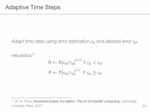
Adaptive Time Steps
Adapt time step using error estimation εa and desired error ϵd.
Heuristics3:h← h
∣∣ϵd/εa∣∣0.25 if εa < ϵd
h← h∣∣ϵd/εa
∣∣0.2 if εa ≥ ϵd
3 W. H. Press, Numerical recipes 3rd edition: The art of scientific computing. CambridgeUniversity Press, 2007. 24
Stiff Systems
Stiff ODEs have time constants (Eigenvalues) differing by afactor of 1000 or more.
Solvers take tiny time steps throughout the entire time horizon
Special solvers are available for stiff ODEs, using implicitmethods to achieve stability at larger time steps.
Ball on String example is stiff for small mass.
25

Ball on String: Stiff for Small Mass
0 0.02 0.04 0.06 0.08 0.1−1
−0.5
0h = 5 · 10−4
h = 2.5 · 10−4
h =
2.5 · 10−4, t ≤ 0.410 · 10−4, t > 0.4x0
t
posit
ionx
0 0.02 0.04 0.06 0.08 0.10
10
20
30
h = 5 · 10−4
h = 2.5 · 10−4
h =
2.5 · 10−4, t ≤ 0.410 · 10−4, t > 0.4
v0
t
veloc
ityv
26
Overview
Hybrid Automata
Numerical Simulation
Solving ODEs
Computing Trajectories and Jumps
Set-Based Reachability
Conclusions
27
Computing Trajectories and Jumps
Numerical simulation of hybrid automata:
• use ODE solver to approximate trajectories,• detect when trajectory enters guard,• detect when trajectory leaves invariant.
ODE solver offer zero crossing detection using root-findingalgorithms.
Detecting guards/invariants using root functions iscomputationally expensive and potentially inaccurate.
28
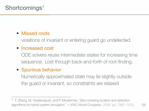
Shortcomings4
• Missed rootsviolations of invariant or entering guard go undetected.
• Increased costODE solvers reuse intermediate states for increasing timesequence. Lost through back-and-forth of root-finding.
• Spurious behaviorNumerically approximated state may lie slightly outsidethe guard or invariant, so constraints are relaxed
4 F. Zhang, M. Yeddanapudi, and P. Mosterman, “Zero-crossing location and detectionalgorithms for hybrid system simulation,” in IFAC World Congress, 2008, pp. 7967–7972. 29
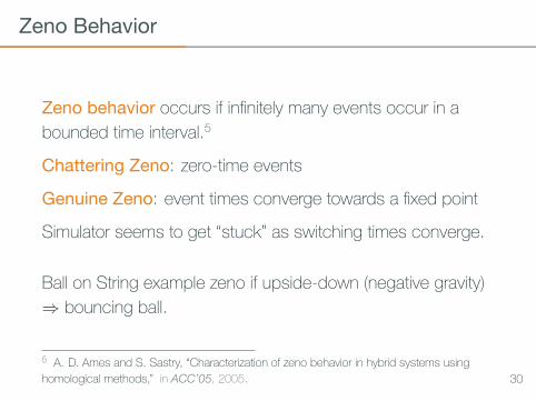
Zeno Behavior
Zeno behavior occurs if infinitely many events occur in abounded time interval.5
Chattering Zeno: zero-time events
Genuine Zeno: event times converge towards a fixed point
Simulator seems to get “stuck” as switching times converge.
Ball on String example zeno if upside-down (negative gravity)⇒ bouncing ball.
5 A. D. Ames and S. Sastry, “Characterization of zeno behavior in hybrid systems usinghomological methods,” in ACC’05, 2005. 30
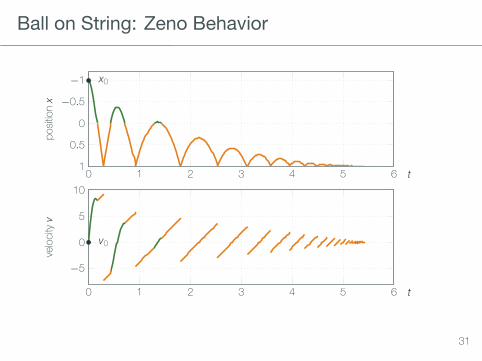
Ball on String: Zeno Behavior
0 1 2 3 4 5 6
−1
−0.5
0
0.5
1
x0
t
posit
ionx
0 1 2 3 4 5 6
−5
0
5
10
v0
t
veloc
ityv
31

Accounting for Nondeterminism
The biggest challenge is nondeterminism:
• select initial state and successor states in jump relation;• choose between transitions if guards overlap;• choose jump time from interval of time;• differential inclusions, such as x ∈ [−1, 1], require to
pick derivative for each time step;
Number of runs increases exponentially with each choice.
Simulators like Simulink, Modelica, or Ptolemy use purelydeterministic models that jump as soon as possible.
32
Overview
Hybrid Automata
Numerical Simulation
Set-Based Reachability
Piecewise Constant Dynamics
Piecewise Affine Dynamics
Set Representations
SpaceEx (advertisement)
Conclusions
33
Set-Based Reachability
Extending numerical simulation from numbers to sets
• account for nondeterminism• exhaustive• infinite time horizon
Downsides:
• only approximate for complex dynamics• generally not scalable in # of variables• trade-off between runtime and accuracy
34

Reachability Algorithm
One-step successors by time elapse from set of states S,
PostC(S) =(ℓ, ξ(δ))
∣∣ ∃(ℓ, x) ∈ S : (ℓ, x) δ,ξ−→ (ℓ, ξ(δ)).
One-step successors by jump from set of states S,
PostD(S) =(ℓ′, x′)
∣∣ ∃(ℓ′, x′) ∈ S,∃α ∈ Lab ∪ τ :(ℓ, x) α−→ (ℓ′, x′)
.
35

Reachability Algorithm
Compute sequence
R0 = PostC(Init),Ri+1 = Ri ∪ PostC(PostD(Ri)).
If Ri+1 = Ri, then Ri = reachable states.
• may not terminate if states unbounded (counter)• problem undecidable in general6
6 T. A. Henzinger, P. W. Kopke, A. Puri, and P. Varaiya, “What’s decidable about hybridautomata?” Journal of Computer and System Sciences, vol. 57, pp. 94–124, 1998. 36
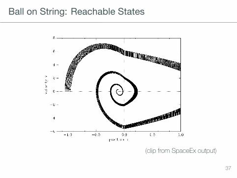
Ball on String: Reachable States
(clip from SpaceEx output)
37
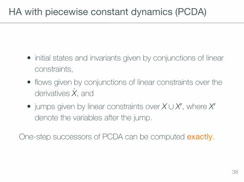
HA with piecewise constant dynamics (PCDA)
• initial states and invariants given by conjunctions of linearconstraints,
• flows given by conjunctions of linear constraints over thederivatives X, and
• jumps given by linear constraints over X ∪ X′, where X′
denote the variables after the jump.
One-step successors of PCDA can be computed exactly.
38
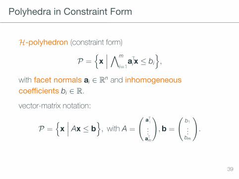
Polyhedra in Constraint Form
H-polyhedron (constraint form)
P =x∣∣∣ ∧m
i=1aT
ix ≤ bi
,
with facet normals ai ∈ Rn and inhomogeneouscoefficients bi ∈ R.
vector-matrix notation:
P =x∣∣∣ Ax ≤ b
, with A =
(aT
1...aT
m
),b =
(b1...
bm
).
39
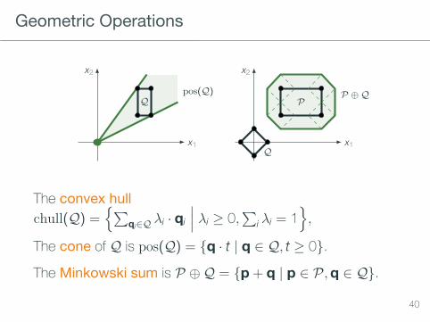
Geometric Operations
0 0.2 0.4 0.6 0.8 100.20.40.60.81
x1
x2
Qpos(Q)
x1
x2
P
Q
P ⊕Q
The convex hullchull(Q) =
∑qi∈Q λi · qi
∣∣∣ λi ≥ 0,∑
i λi = 1,
The cone of Q is pos(Q) = q · t | q ∈ Q, t ≥ 0.
The Minkowski sum is P ⊕Q = p+ q | p ∈ P ,q ∈ Q.
40

Polyhedra in Generator Form
V-polyhedron (generator form)
P = (V,R) = chull (V)⊕ pos(chull(R)).
with vertices V ⊆ Rn and rays R ⊆ Rn
conversion between H- and V-polyhedra is expensive
cube: 2n constraints, 2n vertices
cross-polytope (diamond): 2n vertices, 2n constraints
41

Time Elapse with Polyhedra
For PCDA, it suffices to consider straight-line trajectories:
Lemma (Constant Derivatives7)
There is a trajectory ξ(t) from x = ξ(0) to x′ = ξ(δ), δ > 0, iffη(t) = x+ qt with q = (x′ − x)/δ is a trajectory from x to x′.
7 P.-H. Ho, “Automatic analysis of hybrid systems,” Technical Report CSD-TR95-1536,PhD thesis, Cornell University, Aug. 1995. 42
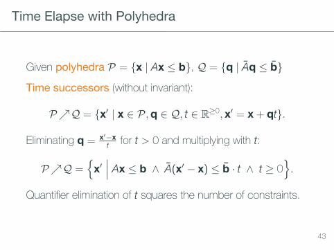
Time Elapse with Polyhedra
Given polyhedra P = x | Ax ≤ b, Q = q | Aq ≤ b
Time successors (without invariant):
PQ = x′ | x ∈ P ,q ∈ Q, t ∈ R≥0, x′ = x+ qt.
Eliminating q = x′−xt for t > 0 and multiplying with t:
PQ =x′∣∣∣ Ax ≤ b ∧ A(x′ − x) ≤ b · t ∧ t ≥ 0
.
Quantifier elimination of t squares the number of constraints.
43
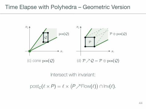
Time Elapse with Polyhedra – Geometric Version
x1
x2
Qpos(Q)
(c) cone pos(Q)
x1
x2
P
P ⊕ pos(Q)
(d) PQ = P ⊕ pos(Q)
Intersect with invariant:
postC(ℓ× P) = ℓ×(PFlow(ℓ)
)∩ Inv(ℓ).
44
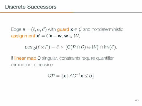
Discrete Successors
Edge e = (ℓ, α, ℓ′) with guard x ∈ G and nondeterministicassignment x′ = Cx+w, w ∈ W,
postD(ℓ× P) = ℓ′ ×(C(P ∩ G)⊕W
)∩ Inv(ℓ′).
If linear map C singular, constraints require quantifierelimination, otherwise
CP = x | AC−1x ≤ b
45

Computational Cost
polyhedraoperation m constraints k generators
cone m2 kMinkowski sum exp k2
linear map m / exp kintersection 2m exp
46
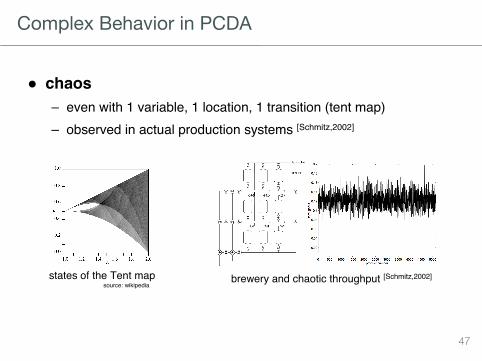
Complex Behavior in PCDA
36
Linear Hybrid Automata
Ɣ chaos– even with 1 variable, 1 location, 1 transition (tent map)– observed in actual production systems [Schmitz,2002]
states of the Tent mapsource: wikipedia
Schmitz, J. P. M., D. A. Van Beek, and J. E. Rooda. "Chaos in discrete production systems?." Journal of Manufacturing Systems 21.3 (2002): 236-246.c
brewery and chaotic throughput [Schmitz,2002]
47
40
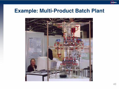
Example: Multi-Product Batch Plant
48
41
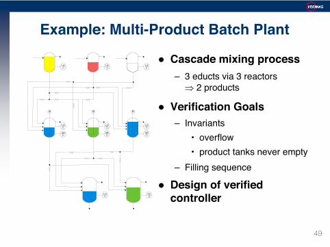
Example: Multi-Product Batch Plant
Ɣ Cascade mixing process– 3 educts via 3 reactors
2 products
Ɣ Verification Goals– Invariants
• overflow• product tanks never empty
– Filling sequence
Ɣ Design of verified controller
LIS11
M
LIS22
QIS22
LIS32
LIS31
M
LIS23
QIS23
M
LIS21
QIS21
LIS13
LIS12
49
42
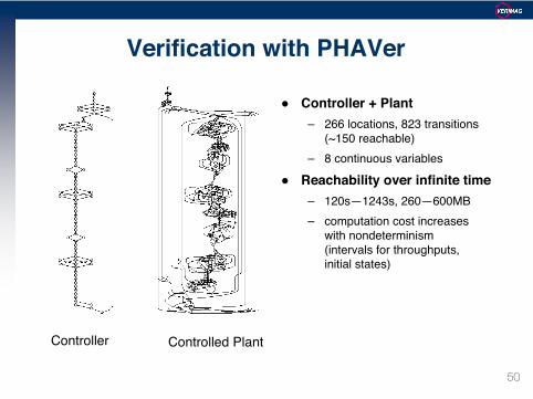
Verification with PHAVer
Ɣ Controller + Plant– 266 locations, 823 transitions
(~150 reachable)– 8 continuous variables
Ɣ Reachability over infinite time– 120s—1243s, 260—600MB– computation cost increases
with nondeterminism(intervals for throughputs, initial states)
Controller Controlled Plant
50
43
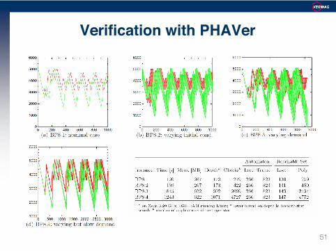
Verification with PHAVer
51
Overview
Hybrid Automata
Numerical Simulation
Set-Based Reachability
Piecewise Constant Dynamics
Piecewise Affine Dynamics
Set Representations
SpaceEx (advertisement)
Conclusions
52

Piecewise Affine Dynamics
Hybrid automata with piecewise affine dynamics (PWA)
• initial states and invariants are polyhedra,• flows are affine ODEs
x = Ax+ Bu, u ∈ U ,
• jumps have a guard set and assignments
x′ = Cx+w, w ∈ W .
53
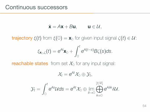
Continuous successors
x = Ax+ Bu, u ∈ U ,
trajectory ξ(t) from ξ(0) = x0 for given input signal ζ(t) ∈ U :
ξx0,ζ(t) = eAtx0 +
∫ t
0eA(t−s)Bζ(s)ds.
reachable states from set X0 for any input signal:
Xt = eAtX0 ⊕ Yt,
Yt =
∫ t
0eAsUds = eAtX0 ⊕ lim
δ→0
⌊t/δ⌋⊕k=0
eAδkδU .
54
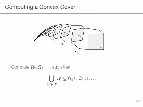
Computing a Convex Cover
X0
Ω0
Xδ
Ω1
X2δ
Ω2
Compute Ω0,Ω1, . . . such that∪0≤t≤T
Xt ⊆ Ω0 ∪ Ω1 ∪ . . . .
55

Time Discretization
X0Ω0
Xδ
Ω1
X2δ
Ω2
Semi-group property: (Xkδ)δ = X(k+1)δ
Time discretization: X(k+1)δ = eAδXkδ ⊕ Yδ.
Given initial approximations Ω0 and Ψδ such that∪0≤t≤δ
Xt ⊆ Ω0, Yδ ⊆ Ψδ,
Xt is covered by the sequenceΩk+1 = eAδΩk ⊕Ψδ.
56
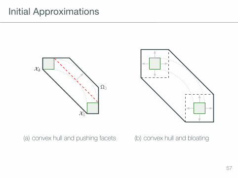
Initial Approximations
X0
Xδ
Ω0
(a) convex hull and pushing facets (b) convex hull and bloating
57
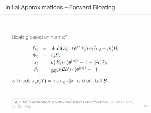
Initial Approximations – Forward Bloating
Bloating based on norms:8
Ω0 = chull(X0 ∪ eAδX0)⊕ (αδ + βδ)B,Ψδ = βδB,αδ = µ(X0) · (e∥A∥δ − 1− ∥A∥δ),βδ = 1
∥A∥µ(BU) · (e∥A∥δ − 1),
with radius µ(X ) = maxx∈X∥x∥ and unit ball B.
8 A. Girard, “Reachability of uncertain linear systems using zonotopes,” in HSCC, 2005,pp. 291–305. 58
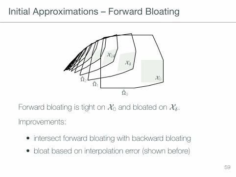
Initial Approximations – Forward Bloating
X0
Ω0
Xδ
Ω1
X2δ
Ω2
Forward bloating is tight on X0 and bloated on Xδ.
Improvements:
• intersect forward bloating with backward bloating• bloat based on interpolation error (shown before)
59
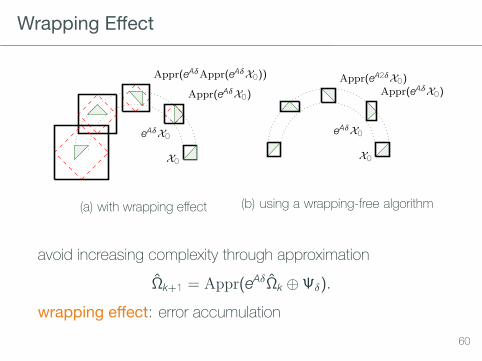
Wrapping Effect
X0
eAδX0
Appr(eAδX0)
Appr(eAδAppr(eAδX0))
(a) with wrapping effect
X0
eAδX0
Appr(eAδX0)Appr(eA2δX0)
(b) using a wrapping-free algorithm
avoid increasing complexity through approximationΩk+1 = Appr(eAδΩk ⊕Ψδ).
wrapping effect: error accumulation60
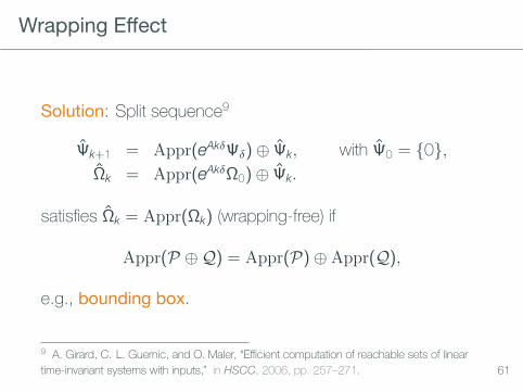
Wrapping Effect
Solution: Split sequence9
Ψk+1 = Appr(eAkδΨδ)⊕ Ψk, with Ψ0 = 0,Ωk = Appr(eAkδΩ0)⊕ Ψk.
satisfies Ωk = Appr(Ωk) (wrapping-free) if
Appr(P ⊕Q) = Appr(P)⊕ Appr(Q),
e.g., bounding box.
9 A. Girard, C. L. Guernic, and O. Maler, “Efficient computation of reachable sets of lineartime-invariant systems with inputs,” in HSCC, 2006, pp. 257–271. 61

Overview
Hybrid Automata
Numerical Simulation
Set-Based Reachability
Piecewise Constant Dynamics
Piecewise Affine Dynamics
Set Representations
SpaceEx (advertisement)
Conclusions
62
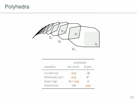
Polyhedra
X0
Ω0
Xδ
Ω1
X2δ
Ω2
polyhedraoperation m constr. k gen.
convex hull exp 2kMinkowski sum exp k2
linear map m / exp kintersection 2m exp
63
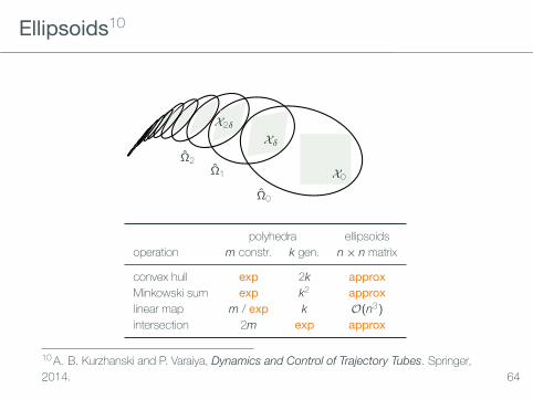
Ellipsoids10
X0
Ω0
Xδ
Ω1
X2δ
Ω2
polyhedra ellipsoidsoperation m constr. k gen. n × n matrix
convex hull exp 2k approxMinkowski sum exp k2 approxlinear map m / exp k O(n3)intersection 2m exp approx
10 A. B. Kurzhanski and P. Varaiya, Dynamics and Control of Trajectory Tubes. Springer,2014. 64

Zonotopes
v1v2
v3
v4c
Zonotope with center c ∈ Rn and generators v1, . . . , vk ∈ Rn
P =
c+
∑k
i=1αivi
∣∣∣∣ αi ∈ [−1, 1].
linear map: map center and generatorsMinkowski sum: add centers, take union of generators
65
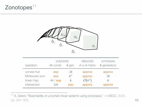
Zonotopes11
X0
Ω0
Xδ
Ω1
X2δ
Ω2
polyhedra ellipsoids zonotopesoperation m constr. k gen. n × n matrix k generators
convex hull exp 2k approx approxMinkowski sum exp k2 approx 2klinear map m / exp k O(n3) kintersection 2m exp approx approx
11 A. Girard, “Reachability of uncertain linear systems using zonotopes,” in HSCC, 2005,pp. 291–305. 66
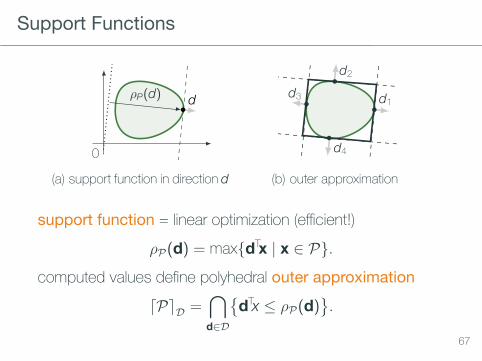
Support Functions
dρP(d)
P
0
(a) support function in direction d
d3
d4
d1
d2
P
⌈P⌉D
(b) outer approximation
support function = linear optimization (efficient!)ρP(d) = maxdTx | x ∈ P.
computed values define polyhedral outer approximation
⌈P⌉D =∩d∈D
dTx ≤ ρP(d)
.
67
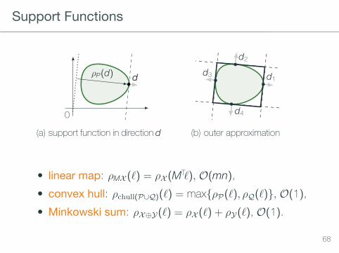
Support Functions
dρP(d)
P
0
(a) support function in direction d
d3
d4
d1
d2
P
⌈P⌉D
(b) outer approximation
• linear map: ρMX (ℓ) = ρX (MTℓ), O(mn),• convex hull: ρchull(P∪Q)(ℓ) = maxρP(ℓ), ρQ(ℓ), O(1),• Minkowski sum: ρX⊕Y(ℓ) = ρX (ℓ) + ρY(ℓ), O(1).
68

Support Functions (Le Guernic, Girard,’09)[13]
X0
Ω0
Xδ
Ω1
X2δ
Ω2X0
Ω0
Xδ
Ω1
X2δ
Ω2
support functions: lazy approximation on demand
polyhedra ellipsoids zonotopes support f.operation m constr. k gen. n × n matrix k generators —
convex hull exp 2k approx approx O(1)Minkowski sum exp k2 approx 2k O(1)linear map m / exp k O(n3) k O(n2)intersection 2m exp approx approx opt. / approx
69
68
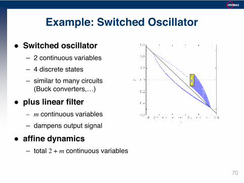
Example: Switched Oscillator
Ɣ Switched oscillator– 2 continuous variables– 4 discrete states– similar to many circuits
(Buck converters,…)
Ɣ plus linear filter– m continuous variables– dampens output signal
Ɣ affine dynamics– total 2 + m continuous variables
70
28
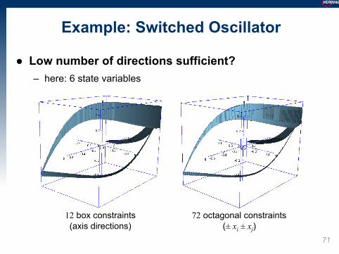
Example: Switched Oscillator
Low number of directions sufficient? – here: 6 state variables
12 box constraints (axis directions)
72 octagonal constraints (± xi ± xj)
71
69
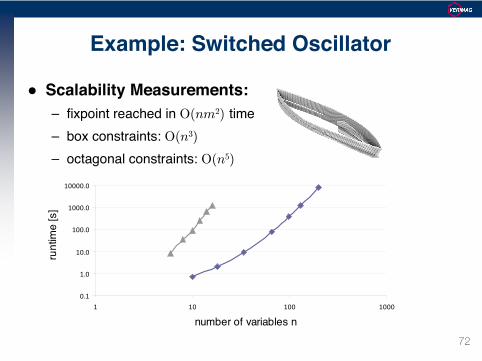
Example: Switched Oscillator
Ɣ Scalability Measurements:– fixpoint reached in O(nm2) time– box constraints: O(n3)
– octagonal constraints: O(n5)
0.1
1.0
10.0
100.0
1000.0
10000.0
1 10 100 1000
number of variables n
runt
ime
[s]
72

85
Example: Controlled Helicopter
Ɣ 28-dim model of a Westland Lynx helicopter– 8-dim model of flight dynamics– 20-dim continuous H' controller for disturbance rejection– stiff, highly coupled dynamics
S. Skogestad and I. Postlethwaite, Multivariable Feedback Control: Analysis and Design. John Wiley & Sons, 2005.
Photo by Andrew P Clarke
73
86
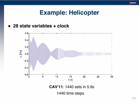
Example: Helicopter
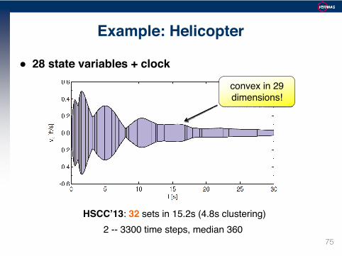
Ɣ 28 state variables + clock
CAV’11: 1440 sets in 5.9s1440 time steps
74
87
Ɣ 28 state variables + clock
Example: Helicopter
HSCC’13: 32 sets in 15.2s (4.8s clustering)2 -- 3300 time steps, median 360
convex in 29 dimensions!convex in 29 dimensions!
75
88
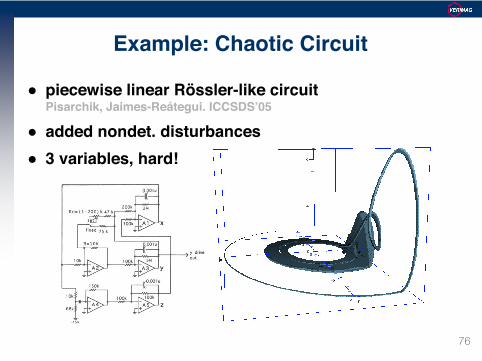
Example: Chaotic Circuit
Ɣ piecewise linear Rössler-like circuitPisarchik, Jaimes-Reátegui. ICCSDS’05
Ɣ added nondet. disturbancesƔ 3 variables, hard!
76

Nonlinear Dynamics – Linearization
x = f(x),
with f globally Lipschitz continuous.
Linearization: choose domain S (partition, sliding window)
overapproximate in S with x = Ax+ u,u ∈ U
linearizing f(x) around x0 ∈ S gives
aij =∂fi∂xj
∣∣∣∣x=x0
and b = f(x0)− Ax0.
U = Appr f(x)− (Ax+ b), x ∈ S ⊕ b.
77
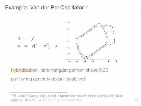
Example: Van der Pol Oscillator12
x = yy = y(1− x2)− x
hybridization: here triangular partition of size 0.05
partitioning generally doesn’t scale well
12 E. Asarin, T. Dang, and A. Girard, “Hybridization methods for the analysis of nonlinearsystems,” Acta Inf., vol. 43, no. 7, pp. 451–476, 2007. 78
Nonlinear Dynamics – Polynomial Approximations
Bernstein polynomials for polynomial f(x)
• polyhedral approximation of successors13
Taylor models
• polynomial approximations of Taylor expansion• represent sets with polynomials• Flow* verification tool[16]
13 T. Dang and R. Testylier, “Reachability analysis for polynomial dynamical systems using thebernstein expansion,” Reliable Computing, vol. 17, no. 2, pp. 128–152, 2012. 79

Overview
Hybrid Automata
Numerical Simulation
Set-Based Reachability
Piecewise Constant Dynamics
Piecewise Affine Dynamics
Set Representations
SpaceEx (advertisement)
Conclusions
80
90
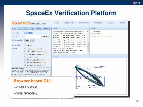
SpaceEx Verification Platform
Browser-based GUI–2D/3D output–runs remotely
81

91
SpaceEx Model Editor
Components = Hybrid Automata– real-values variables– ODE, linear DAE
82
92
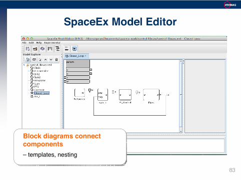
SpaceEx Model Editor
Block diagrams connect components– templates, nesting
83
93
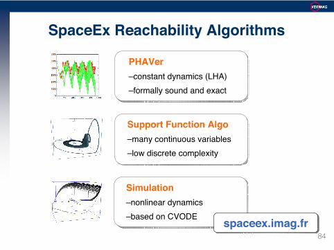
PHAVer–constant dynamics (LHA)–formally sound and exact
SpaceEx Reachability Algorithms
Support Function Algo–many continuous variables–low discrete complexity
Simulation–nonlinear dynamics–based on CVODE
spaceex.imag.frspaceex.imag.fr84

Overview
Hybrid Automata
Numerical Simulation
Set-Based Reachability
Conclusions
85
Conclusions
• Hybrid systems are easy to model with hybrid automatabut difficult to analyze.
• Numerical simulation scales, but is not exhaustive andcritical behavior may be missed.
• Set-based reachability covers all runs, sufficient forsafety and bounded liveness.
• computational cost,• scalable for piecewise affine dynamics
• Remaining challenges: trade-off between approximationaccuracy and computational cost, scalable extension tononlinear dynamics
86
References I
[2] R. Alur, C. Courcoubetis, N. Halbwachs, T. Henzinger, P.-H. Ho, X. Nicollin,A. Olivero, J. Sifakis, and S. Yovine, “The algorithmic analysis of hybrid systems,”Theoretical Computer Science, vol. 138, pp. 3–34, 1995.
[3] T. A. Henzinger, “The theory of hybrid automata.,” in LICS, Los Alamitos: IEEEComputer Society, 1996, pp. 278–292.
[13] C. Le Guernic and A. Girard, “Reachability analysis of linear systems using supportfunctions,” Nonlinear Analysis: Hybrid Systems, vol. 4, no. 2, pp. 250–262, 2010.
[16] X. Chen, E. Ábrahám, and S. Sankaranarayanan, “Taylor model flowpipe constructionfor non-linear hybrid systems,” in RTSS, IEEE Computer Society, 2012,pp. 183–192, ISBN: 978-1-4673-3098-5.
87


![A cellular learning automata based algorithm for detecting ... · by combining cellular automata (CA) and learning automata (LA) [22]. Cellular learning automata can be defined as](https://img.pdfslide.us/doc/110x75/601a3ee3c68e6b5bec07f1bb/a-cellular-learning-automata-based-algorithm-for-detecting-by-combining-cellular.jpg)