Embed Size (px)
Citation preview
An Introduction toHILBERT-HUANG TRANSFORM
and EMPIRICAL MODE DECOMPOSITION
(HHT-EMD)
Advanced Structural Dynamics
(CE 20162)
M. Ahmadizadeh, PhD, PE
O. Hemmati
1

Contents
• Scope and Goals
• Review on transformations
– STFT
– WAVELET
• Introduction
• HHT
• IMF
• EMD
– limitations
• Comparison b/w transformers
2
Scope and Goals
• Need a basis that determined through signal characteristics , not by user prior to the analysis.
• Need transformation that be able to overcome Heisenberg uncertainty theorem which is restricted resolution.
• Need to noise subtraction.
3

Review on transformations
• TRADITIONAL FOURIER
• STFT:
– which allow a signal to be nonstationary as long as it is piece-wise stationary
• WAVELET
– which can sift out particular signatures from a signal on a variety of size scales
• HHT
4

• General STFT
• Gabor Transform
Gaussian window function minimizes the Fourier uncertainty principle. (Gabor transform with modifications for multi-resolution becomes the Morlet wavelet transform).
• Generalized Time-Frequency Distributions
Overall, the Wigner-Ville distribution gives better time and frequency resolution than STFT and does not have to sacrifice one resolution for the benefit of the other.
STFT
5

WAVELET
• This was an improvement over STFT because, as the result of the flexible basis functions, both the high-frequency and the low-frequency structures could be analyzed.
• However, a drawback of wavelet analysis is that the wavelet basis functions, and therefore the structures being sifted out from the original signal, are chosen a priori.
• It is possible that the utilized wavelets may or may not reflect the processes in the analyzed signal.
6

Introduction
• HHT is able to extract the frequency components from possibly nonlinear and nonstationary intermittent signals
• HHT is able to overcome Heisenberg uncertainty theorem which is restricted resolution of Fourier transformation.
• HHT has been used to study a wide variety of data including rainfall, earthquakes, heart-rate variability, financial time series, Lidar data, and ocean waves to name a few subjects.
7

HHT
Hilbert transform is developed the unique and physical definitions of instantaneous frequency and instantaneous amplitude of a signal but with different physical explanation of frequency , generalized from the conventional Fourier definition.
𝑌 𝑡 = 𝐻 𝑥 𝑡 =1
𝜋 −∞
+∞ 𝑥 𝜏
𝑡 − 𝜏𝑑𝜏
𝑥(𝑡) arbitrary real signal𝑌 𝑡 Hilbert transform of 𝑥 𝑡𝑍 𝑡 analytic signal of 𝑥 𝑡 in polar coordinate representation
𝑍 𝑡 = 𝑥 𝑡 + 𝑖𝑌 𝑡 = 𝑎 𝑡 𝑒𝑖𝜃 𝑡
𝑎 𝑡 = 𝑥2 𝑡 + 𝑌2 𝑡 1/2
𝜃 𝑡 = 𝑎𝑟𝑐𝑡𝑎𝑛𝑌 𝑡
𝑥 𝑡𝜔 𝑡 = 𝜃′ 𝑡
𝜔 𝑡 is dominated as instantaneous frequency 𝑎 𝑡 the instantaneous amplitude
8

Mathematical Properties of Hilbert
• Linearity
• Inverse of Hilbert Transform𝐻2 = 𝐼𝐻3 = 𝐻−1
• Derivatives of Hilbert Transform𝐻 𝑓′ 𝑡 = 𝐻′ 𝑓 𝑡
• Orthogonality
9
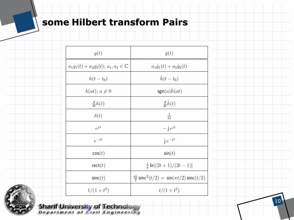
some Hilbert transform Pairs
10

Comparison b/w transformers (.wiki)
Transform Fourier Wavelet Hilbert
Basis a priori a priori adaptive
Frequencyconvolution: global, uncertainty
convolution: regional, uncertainty
differentiation: local, certainty
Presentationenergy-frequency
energy-time-frequency
energy-time-frequency
Nonlinear no no yes
Non-stationary no yes yes
Feature Extraction
nodiscrete: no, continuous: yes
yes
Theoretical Base
theory complete
theory complete
empirical
11

HHT
• not all functions give “good” Hilbert transforms, meaning those which produce physical instantaneous frequencies.
• It is essentially an algorithm which decomposes nearly any signal into a finite set of functions which have “good” Hilbert transforms that produce physically meaningful instantaneous frequencies.
• For this purposes, the empirical mode decomposition was introduced.
12

IMF
1- the number of local extrema and the number of zero crossings must either equal or differ at most by one;
2- at any point, the mean value of the envelope defined by local maxima and the envelope defined by local minima is zero.
Any signal satisfying these two conditions is called an intrinsic mode function (IMF)
13
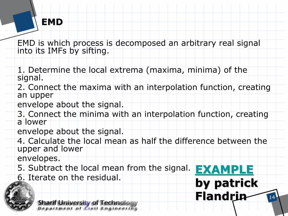
EMD
EMD is which process is decomposed an arbitrary real signal into its IMFs by sifting.
1. Determine the local extrema (maxima, minima) of the signal.2. Connect the maxima with an interpolation function, creating an upperenvelope about the signal.3. Connect the minima with an interpolation function, creating a lowerenvelope about the signal.4. Calculate the local mean as half the difference between the upper and lowerenvelopes.5. Subtract the local mean from the signal.6. Iterate on the residual.
14
EXAMPLEby patrickFlandrin

Limitations for IF computed through Hilbert Transform
• Data must be expressed in terms of Intrinsic Mode Function. IMF is only necessary but not sufficient.
• Bedrosian Theorem: Hilbert transform of a(t) cos θ(t)might not be exactly a(t) sin θ(t). Spectra of a(t) and cos θ(t) must be disjoint.
• Nuttall Theorem: Hilbert transform of cos θ(t) might not be sin θ(t) for an arbitrary function of θ(t). Quadrature and Hilbert Transform of arbitrary real functions are not necessarily identical.
• Therefore, a simple derivative of the phase of the analytic function for an arbitrary function may not work.
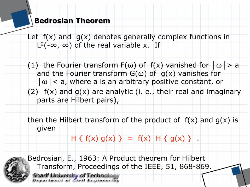
Bedrosian Theorem
Let f(x) and g(x) denotes generally complex functions in L2(-∞, ∞) of the real variable x. If
(1) the Fourier transform F(ω) of f(x) vanished for │ω│> a and the Fourier transform G(ω) of g(x) vanishes for │ω│< a, where a is an arbitrary positive constant, or
(2) f(x) and g(x) are analytic (i. e., their real and imaginary
parts are Hilbert pairs),
then the Hilbert transform of the product of f(x) and g(x) is given
H { f(x) g(x) } = f(x) H { g(x) } .
Bedrosian, E., 1963: A Product theorem for Hilbert Transform, Proceedings of the IEEE, 51, 868-869.
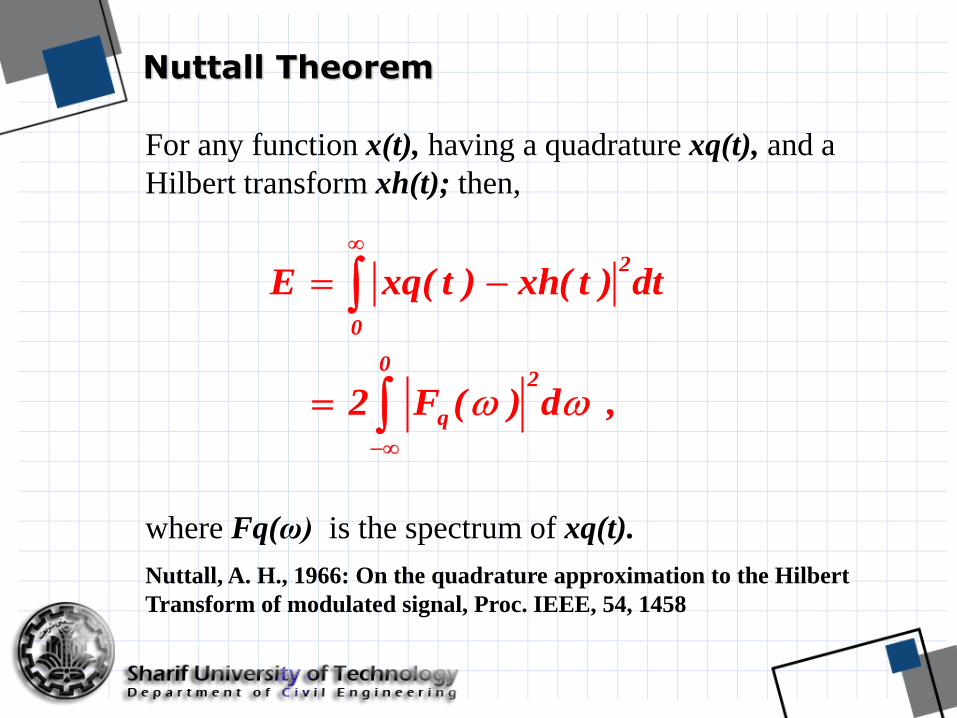
Nuttall Theorem
For any function x(t), having a quadrature xq(t), and a
Hilbert transform xh(t); then,
where Fq(ω) is the spectrum of xq(t).
Nuttall, A. H., 1966: On the quadrature approximation to the Hilbert
Transform of modulated signal, Proc. IEEE, 54, 1458
2
0
02
q
E xq( t ) xh( t ) dt
2 F ( ) d ,

Difficulties with the Existing Limitations
• Data are not necessarily IMFs.
• Even if we use EMD to decompose the data into IMFs. IMF is only necessary but not sufficient because of the following limitations:
• Bedrosian Theorem adds the requirement of not having strong amplitude modulations.
• Nuttall Theorem further points out the difference between analytic function and quadrature.
• The discrepancy, however, is given in term of the quadrature spectrum, which is an unknown quantity. Therefore, it cannot be evaluated. Nuttall Theorem provides a constant limit not a function of time; therefore, it is not very useful for non-stationary processes.

Analytic vs. Quadrature
X(t)
Y(t) Z(t) Analytic
Hilbert Transform
Q(t) Quadrature, not analytic
No Known general method
Analytic functions satisfy Cauchy-Reimann equation, but may be x2+ y2
≠ 1. Then the arc-tangent would not recover the true phase function.
Quadrature pairs are not analytic, but satisfy strict 90o phase shift;
therefore, x2+ y2 = 1, and the arc-tangent always gives the true phase
function.
For cosθ(t) with arbitrary function of θ(t) :

Other Limitations
The EMD has limitations in distinguishing components in narrowband signals.
1- End effect issue,
2- Order of the IMF extractions,
3- EMD’s unsatisfactory resolution.
20

example
[Chen, 2003]proposes a new method to eliminate this problem
21

Example
22

Sunspot number data set
23

Total solar Irradiance measurements
24
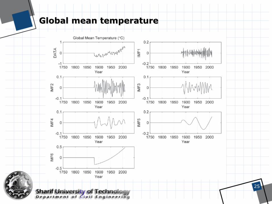
Global mean temperature
25

CO2 Concentration
26

Subsection of IM2
27

Comparison b/w TSI and sunspot number IMF
28

Comparison of IMFs for global mean temperature and TSI
29

Comparison of IMFs for global mean temperature and sunspot number data
30

Correlation Coeff. TSI and sunspot/GMT
31

Correlation Coeff. GMT and TSI/sunspot
32

Correlation Coeff. GMT and sunspot
33

Gibbs Effect (.wiki)
• In non-continuous signal with an abrupt discontinuity, when finite number of Fourier coefficients was used, Gibbs phenomenon was occurred.
• All of 3 mentioned transforms suffers this effect.
• Wavelets are more useful for describing these signals with discontinuities because of their time-localized behavior (both Fourier and wavelet transforms are frequency-localized, but wavelets have an additional time-localization property). Because of this, many types of signals in practice may be non-sparse in the Fourier domain, but very sparse in the wavelet domain.
• For HHT could be used more sophisticated methods, such as Riesz basis, to avoid the Gibbs phenomenon.
• The reducing methods of this phenomenon for Fourier, were introduced in [Hamming 2003]
34
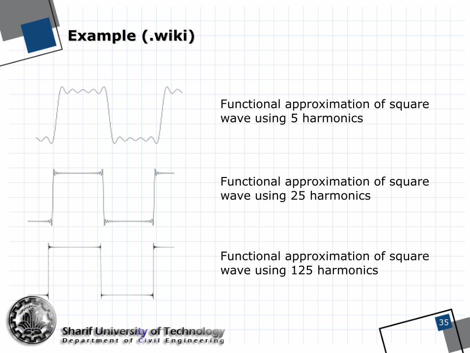
Example (.wiki)
35
Functional approximation of square wave using 5 harmonics
Functional approximation of square wave using 25 harmonics
Functional approximation of square wave using 125 harmonics

HHT implementation
• commercial software called the Hilbert-Huang transform data processing system (HHT-DPS) which was developed by Norden Huang at NASA and is available through NASA’s website.
• There are also publicly available Matlab codes by Patrick Flandrin and R code which extract IMFs from a given input data series.
36

REFERENCES
1. Chen, Yangbo, and Maria Q. Feng. "A technique to improve the empirical mode decomposition in the Hilbert-Huang transform." Earthquake Engineering and Engineering Vibration 2.1 (2003): 75-85.
2. Hamming, Richard R. Art of Doing Science and Engineering: Learning to Learn. CRC Press, 2003.
3. Adcock, Ben, and Anders C. Hansen. "Stable reconstructions in Hilbert spaces and the resolution of the Gibbs phenomenon." Applied and Computational Harmonic Analysis 32.3 (2012): 357-388.
4. Cheng, CK. " Lecture 12-13 Hilbert-Huang Transform Background " (Spring 2014) Topics on Numeric Methods for Biosignal Processing , University of California, San Diego.
5. Wang, Yung-Hung, et al. "On the computational complexity of the empirical mode decomposition algorithm." Physica A: Statistical Mechanics and its Applications 400 (2014): 159-167.
6. http://perso.ens-lyon.fr/patrick.flandrin/emd.html retrieved (04-03-2015)
7. http://en.wikipedia.org/wiki/Wavelet retrieved (04-03-2015)
8. http://en.wikipedia.org/wiki/Gibbs_phenomenon retrieved (04-03-2015)
37