Embed Size (px)
Citation preview

AN INTRODUCTION TO
HARMONICANALYSIS
Yitzhak Katznelson
Third Corrected Edition


Preface
Harmonic analysis is the study of objects (functions, measures, etc.),defined on topological groups. The group structure enters into the studyby allowing the consideration of the translates of the object under study,that is, by placing the object in a translation-invariant space. The studyconsists of two steps. First: finding the "elementary components" ofthe object, that is, objects of the same or similar class, which exhibitthe simplest behavior under translation and which "belong" to the ob-ject under study (harmonic or spectralanalysis); and second: findinga way in which the object can be construed as a combination of itselementary components (harmonic or spectralsynthesis).
The vagueness of this description is due not only to the limitationof the author but also to the vastness of its scope. In trying to make itclearer, one can proceed in various ways†; we have chosen here to sac-rifice generality for the sake of concreteness. We start with the circlegroupT and deal with classical Fourier series in the first five chap-ters, turning then to the real line in Chapter VI and coming to locallycompact abelian groups, only for a brief sketch, in Chapter VII. Thephilosophy behind the choice of this approach is that it makes it easierfor students to grasp the main ideas and gives them a large class of con-crete examples which are essential for the proper understanding of thetheory in the general context of topological groups. The presentation ofFourier series and integrals differs from that in [1], [7], [8], and [28] inbeing, I believe, more explicitly aimed at the general (locally compactabelian) case.
The last chapter is an introduction to the theory of commutativeBanach algebras. It is biased, studying Banach algebras mainly as atool in harmonic analysis.
This book is an expanded version of a set of lecture notes written
†Hence the indefinite article in the title of the book.
iii

IV AN INTRODUCTION TOHARMONIC ANALYSIS
for a course which I taught at Stanford University during the springand summer quarters of 1965. The course was intended for graduatestudents who had already had two quarters of the basic "real-variable"course. The book is on the same level: the reader is assumed to be fa-miliar with the basic notions and facts of Lebesgue integration, the mostelementary facts concerning Borel measures, some basic facts aboutholomorphic functions of one complex variable, and some elements offunctional analysis, namely: the notions of a Banach space, continuouslinear functionals, and the three key theorems—"the closed graph", theHahn-Banach, and the "uniform boundedhess" theorems. All the pre-requisites can be found in [23] and (except, for the complex variable)in [22]. Assuming these prerequisites, the book, or most of it, can becovered in a one-year course. A slower moving course or one shorterthan a year may exclude some of the starred sections (or subsections).Aiming for a one-year course forced the omission not only of the moregeneral setup (non-abelian groups are not even mentioned), but also ofmany concrete topics such as Fourier analysis onRn, n > l, and finerproblems of harmonic analysis inT or R (some of which can be foundin [13]). Also, some important material was cut into exercises, and weurge the reader to do as many of them as he can.
The bibliography consists mainly of books, and it is through the bib-liographies included in these books that the reader is to become famil-iar with the many research papers written on harmonic analysis. Onlysome, more recent, papers are included in our bibliography. In generalwe credit authors only seldom—most often for identification purposes.With the growing mobility of mathematicians, and the happy amountof oral communication, many results develop within the mathematicalfolklore and when they find their way into print it is not always easyto determine who deserves the credit. When I was writing Chapter Illof this book, I was very pleased to produce the simple elegant proof ofTheorem 1.6 there. I could swear I did it myself until I rememberedtwo days later that six months earlier, "over a cup of coffee," LennartCarleson indicated to me this same proof.
The book is divided into chapters, sections, and subsections. Thechapter numbers are denoted by roman numerals and the sections andsubsections, as well as the exercises, by arabic numerals. In cross ref-erences within the same chapter, the chapter number is omitted; thusTheorem llI.1.6, which is the theorem in subsection 6 of Section 1of Chapter Ill, is referred to as Theorem 1.6 within Chapter IlI, and

PREFACE V
Theorem Ill.1.6 elsewhere. The exercises are gathered at the end of thesections, and exercise V.1.1 is the first exercise at the end of Section 1,Chapter V. Again, the chapter number is omitted when an exercise isreferred to within the same chapter. The ends of proofs are marked bya triangle (J).
The book was written while I was visiting the University of Parisand Stanford University and it owes its existence to the moral and tech-nical help 1 was so generously given in both places. During the writingI have benefitted from the advice and criticism of many friends; 1 wouldlike to thank them all here. Particular thanks are due to L. Carleson, K.DeLeeuw, J.-P. Kahane, O.C. McGehee, and W. Rudin. I would alsolike to thank the publisher for the friendly cooperation in the productionof this book.
Y ITZHAK KATZNELSON
JerusalemApril 1968
The 2002 edition
The second edition was essentially identical with the first, except forthe correction of a few misprints. The current edition has some moremisprints and “miswritings” corrected, and some material added: anadditional section in the first chapter, a few exercises, and an additionalappendix. The added material does not reflect the progress in the fieldin the past thirty or forty years. Almost all of it could, and should havebeen included in the first edition of the book.
StanfordMarch 2002


Contents
I Fourier Series onT 11 Fourier coefficients . . . . . . . . . . . . . . . . . . . . 22 Summability in norm and homogeneous banach
spaces onT . . . . . . . . . . . . . . . . . . . . . . . . 83 Pointwise convergence ofσn(f). . . . . . . . . . . . . . 184 The order of magnitude of
Fourier coefficients . . . . . . . . . . . . . . . . . . . . 235 Fourier series of square summable functions . . . . . . 286 Absolutely convergent fourier series . . . . . . . . . . . 327 Fourier coefficients of linear functionals . . . . . . . . 358 Additional comments and applications . . . . . . . . . 49
II The Convergence of Fourier Series 601 Convergence in norm . . . . . . . . . . . . . . . . . . . 602 Convergence and divergence at a point . . . . . . . . . 65?3 Sets of divergence . . . . . . . . . . . . . . . . . . . . . 69
III The Conjugate Function 761 The conjugate function . . . . . . . . . . . . . . . . . . 762 The maximal function of Hardy and Littlewood . . . . 893 The Hardy spaces . . . . . . . . . . . . . . . . . . . . . 98
IV Interpolation of Linear Operators 1101 Interpolation of norms and of linear operators . . . . . 1102 The theorem of Hausdorff-Young . . . . . . . . . . . . 116
V Lacunary Series and Quasi-analytic Classes 1221 Lacunary series . . . . . . . . . . . . . . . . . . . . . . 122?2 Quasi-analytic classes . . . . . . . . . . . . . . . . . . . 130
vii

VIII AN INTRODUCTION TOHARMONIC ANALYSIS
VI Fourier Transforms on the Line 1371 Fourier transforms forL1(R) . . . . . . . . . . . . . . . 1382 Fourier-Stieltjes transforms. . . . . . . . . . . . . . . . 1493 Fourier transforms inLp(R); 1 < p ≤ 2. . . . . . . . . . 1604 Tempered distributions and pseudo-measures . . . . . 1675 Almost-Periodic functions on the line . . . . . . . . . 1756 The weak-star spectrum of bounded functions . . . . . 1897 The Paley–Wiener theorems . . . . . . . . . . . . . . . 193?8 The Fourier-Carleman transform . . . . . . . . . . . . . 1989 Kronecker’s theorem . . . . . . . . . . . . . . . . . . . 201
VII Fourier Analysis on Locally CompactAbelian Groups 206
1 Locally compact abelian groups . . . . . . . . . . . . . 2062 The Haar measure . . . . . . . . . . . . . . . . . . . . 2073 Characters and the dual group . . . . . . . . . . . . . . 2084 Fourier transforms . . . . . . . . . . . . . . . . . . . . 2105 Almost-periodic functions and the Bohr
compactification . . . . . . . . . . . . . . . . . . . . . . 211
VIII Commutative Banach Algebras 2141 Definition, examples, and elementary properties . . . . 2142 Maximal ideals and multiplicative
linear functionals . . . . . . . . . . . . . . . . . . . . . 2183 The maximal-ideal space and the
Gelfand representation . . . . . . . . . . . . . . . . . . 2254 Homomorphisms of Banach algebras . . . . . . . . . . 2335 Regular algebras . . . . . . . . . . . . . . . . . . . . . . 2416 Wiener’s general Tauberian theorem . . . . . . . . . . . 2467 Spectral synthesis in regular algebras . . . . . . . . . . 2498 Functions that operate in regular
Banach algebras . . . . . . . . . . . . . . . . . . . . . . 2559 The algebraM(T) and functions that operate on
Fourier-Stieltjes coefficients . . . . . . . . . . . . . . . 26410 The use of tensor products . . . . . . . . . . . . . . . . 269
A Vector-Valued Functions 2771 Riemann integration . . . . . . . . . . . . . . . . . . . 2772 Improper integrals . . . . . . . . . . . . . . . . . . . . . 2783 More general integrals . . . . . . . . . . . . . . . . . . 278

CONTENTS IX
4 Holomorphic vector-valued functions . . . . . . . . . . 278
B Probabilistic Methods 2801 Random series . . . . . . . . . . . . . . . . . . . . . . . 2802 Fourier coefficients of continuous functions . . . . . . 2833 Paley–Zygmund,
(
when∑
|an|2 =∞)
. . . . . . . . . 284
Bibliography 287
Index 289

Symbols
HC(D), 215A(T), 32Br,pq , 57Bc, 14C(T), 14Cn(T), 14Cm+η(T), 49C1∗(T), 49
Cr∗(B), 50Cr∗(B, `
q), 57Cr∗(T), 49Dn, 13En(ϕ), 49En(f,B), 50M(T), 38Pinv, 41S[µ], 35S[f ], 3Sn(µ), 37Sn(µ, t), 37Sn(f), 13Wn(f), 50Λ∗, 49Lipα(T), 16Ω(f, h), 26H, 28Hf , 41Tm,n, 49Tn, 49δ, 38δτ , 38f(n), 3χX , 158
lipα(T), 17L1(T), 2L∞(T), 16Lp(T), 15µf , 41ω(f, h), 26σn(µ), 37σn(µ, t), 37σn(f), 12σn(f, t), 12Jn(t), 16Kn, 12P(r, t), 16Vn(t), 15Trimλ, 282rn, 281˜S[f ], 3f ∗ g, 5f ∗Mg, 183
fτ , 4D, 207R, 1T, 1Z, 1D, 210
x

AN INTRODUCTION TO
HARMONIC ANALYSIS

Chapter I
Fourier Series onT
We denote byR the additive group of real numbers and byZ thesubgroup consisting of the integers. The groupT is defined as the quo-tient R/2πZ where, as indicated by the notation,2πZ is the group ofthe integral multiples of2π. There is an obvious identification betweenfunctions onT and2π-periodic functions onR, which allows an im-plicit introduction of notions such as continuity, differentiability, etc.for functions onT. TheLebesgue measureon T, also, can be definedby means of the preceding identification: a functionf is integrable onT if the corresponding2π-periodic function, which we denote again byf , is integrable on[0, 2π) and we set
∫
Tf(t)dt =
∫ 2π
0
f(x)dx.
In other words, we consider the interval[0, 2π) as a model forT and theLebesgue measuredt onT is the restriction of the Lebesgue measure ofR to [0, 2π). The total mass ofdt onT is equal to2π and many of ourformulas would be simpler if we normalizeddt to have total mass 1,that is, if we replace it bydx/2π. Taking intervals onR as "models" forT is very convenient, however, and we choose to putdt = dx in order toavoid confusion. We "pay" by having to write the factor1/2π in frontof every integral.
An all-important property ofdt on T is its translation invariance,that is, for allt0 ∈ T andf defined onT,
∫
f(t− t0)dt =∫
f(t)dt†
†Throughout this chapter, integrals with unspecified limits of integration are takenoverT.
1

2 AN INTRODUCTION TOHARMONIC ANALYSIS
1 FOURIER COEFFICIENTS
1.1 We denote byL1(T) the space of all (equivalence† classes of)complex-valued, Lebesgue integrable functions onT. For f ∈ L1(T)we put
‖f‖L1 =1
2π
∫
T|f(t)|dt.
It is well known thatL1(T), with the norm so defined, is a Banachspace.
DEFINITION: A trigonometric polynomialonT is an expression of theform
(1.1) P ∼N∑
n=−N
aneint.
The numbersn appearing in (1.1) are called the frequencies ofP ; thelargest integern such that|an| + |a−n| 6= 0 is calledthe degree ofP .The values assumed by the indexn are integers so that each of thesummands in (1.1) is a function onT. Since (1.1) is a finite sum, itrepresents a function, which we denote again byP , defined for eacht ∈ T by
(1.2) P (t) =N∑
n=−N
aneint.
LetP be defined by (1.2). Knowing the functionP we can computethe coefficientsan by the formula
(1.3) an =1
2π
∫
P (t)e−intdt
which follows immediately from the fact that for integers j,
12π
∫
eijtdt =
1 if j = 0,
0 if j 6= 0.
Thus we see that the functionP determines the expression (1.1)and there seems to be no point in keeping the distinction between theexpression (1.1) and the functionP ; we shall consider trigonometricpolynomials as both formal expressions and functions.
†f ∼ g if f(t) = g(t) almost everywhere

I. FOURIER SERIES ONT 3
1.2 DEFINITION: A trigonometric series onT is an expression ofthe form
(1.4) S ∼∞∑
n=−∞ane
int.
Again,n assumes integral values; however, the number of terms in (1.4)may be infinite and there is no assumption whatsoever about the sizeof the coefficients or about convergence. The conjugate‡ of the series(1.4) is, by definition, the series
S ∼∞∑
n=−∞−i sgn(n)aneint.
where sgn(n) = 0 if n = 0 and sgn(n) = n/|n| otherwise.
1.3 Let f ∈ L1(T). Motivated by (1.3) we define thenth Fouriercoefficient off by
(1.5) f(n) =1
2π
∫
f(t)e−intdt.
DEFINITION: The Fourier seriesS[f ] of a functionf ∈ L1(T) is thetrigonometric series
S[f ] ∼∞∑
−∞f(n)eint.
The series conjugate toS[f ] will be denoted by˜S[f ] and referred toas the conjugate Fourier series off . We shall say that a trigonometricseries is a Fourier series if it is the Fourier series of somef ∈ L1(T).
1.4 We turn to some elementary properties of Fourier coefficients.
Theorem. Let f, g ∈ L1(T), then
(a) (f + g)(n) = f(n) + g(n).
(b) For any complex numberα
(αf)(n) = αf(n).
(c) If f is the complex conjugate§ of f then ˆf(n) = f(−n).
‡See Chapter III for motivation of the terminology.§Defined by:f(t) = f(t)) for all t ∈ T.

4 AN INTRODUCTION TOHARMONIC ANALYSIS
(d) Denotefτ (t) = f(t− τ), τ ∈ T; then
fτ (n) = f(n)e−inτ .
(e) |f(n)| ≤ 12π
∫
|f(t)|dt = ‖f‖L1
The proofs of (a) through (e) follow immediately from (1.5) and thedetails are left to the reader.
1.5 Corollary. Assumefj ∈ L1(T), j = 0, 1, . . . , and‖fj−f0‖L1 → 0.Thenf(n)→ f0(n) uniformly.
1.6 Theorem. Let f ∈ L1(T), assumef(0) = 0, and define
F (t) =∫ t
0
f(τ)dτ.
ThenF is continuous,2π-periodic, and
(1.6) F (n) =1inf(n), n 6= 0.
PROOF: The continuity (and, in fact, the absolute continuity) ofF isevident. The periodicity follows from
F (t+ 2π)− F (t) =∫ t+2π
t
f(τ)dτ = 2πf(0) = 0,
and (1.6) is obtained through integration by parts:
F (n) =1
2π
∫ 2π
0
F (t)e−intdt =−12π
∫ 2π
0
F ′(t)1−in
e−intdt =1inf . J
1.7 We now define the convolution operation inL1(T). The readerwill notice the use of the group structure ofT and of the invariance ofdt in the subsequent proofs.
Theorem. Letf, g ∈ L1(T). For almost allt, the functionf(t− τ)g(τ)is integrable (as a function ofτ onT), and, if we write
(1.7) h(t) =1
2π
∫
f(t− τ)g(τ)dτ,
thenh ∈ L1(T) and
(1.8) ‖h‖L1 ≤ ‖f‖L1‖g‖L1 .
Moreover
(1.9) h(n) = f(n)g(n) for all n.

I. FOURIER SERIES ONT 5
PROOF: The functionsf(t− τ) andg(τ), considered as functions of thetwo variables(t, x), are clearly measurable, hence so is
F (t, τ) = f(t− τ)g(τ).
For everyτ , F (t, τ) is just a constant multiple offτ , hence integrabledt, and
12π
∫ (
12π
∫
|F (t, τ)|dt)
dτ =1
2π
∫
|g(τ)|·‖f‖L1dτ = ‖f‖L1‖g‖L1
Hence, by the theorem of Fubini,f(t−τ)g(τ) is integrable (over(0, 2π))as a function ofτ for almost allt, and
12π
∫
|h(t)|dt =1
2π
∫∣
∣
∣
12π
∫
F (t, τ)dτ∣
∣
∣dt ≤1
4π2
∫∫
|F (t, τ)|dt dτ
= ‖f‖L1‖g‖L1
which establishes (1.8). In order to prove (1.9) we write
h(n) =1
2π
∫
h(t)e−intdt =1
4π2
∫∫
f(t− τ)e−in(t−τ)g(τ)e−inτdt dτ
=1
2π
∫
f(t)e−intdt· 12π
∫
g(τ)e−inτdτ = f(n)g(n).
As above the change in the order of integration is justified by Fubini’stheorem. J
1.8 DEFINITION: The convolutionf ∗ g of the (L1(T) functions)fandg is the functionh defined by (1.8). Using the star notation for theconvolution, we can write (1.9):
(1.10) f ∗ g(n) = f(n)g(n).
Theorem. The convolution operation inL1(T) is commutative, asso-ciative, and distributive (with respect to the addition).
PROOF: The change of variableϑ = t− τ gives
12π
∫
f(t− τ)g(τ)dτ =1
2π
∫
g(t− ϑ)f(ϑ)dϑ,
that is,f ∗ g = g ∗ f.

6 AN INTRODUCTION TOHARMONIC ANALYSIS
If f1, f2, f3 ∈ L1(T), then
[(f1 ∗ f2)∗f3](t) =1
4π2
∫∫
f1(t− u− τ)f2(u)f3(τ)du dτ =
14π2
∫∫
f1(t− ω)f2(ω − τ)f3(τ)dω dτ = [f1 ∗ (f2 ∗ f3)](t).
Finally, the distributive law
f1 ∗ (f2 + f3) = f1 ∗ f2 + f1 ∗ f3
is evident from (1.7). J
1.9 Lemma. Assumef ∈ L1(T) and letϕ(t) = eint for some integern. Then
(ϕ ∗ f)(t) = f(n)eint.
PROOF:
(ϕ ∗ f)(t) =1
2π
∫
ein(t−τ)f(τ)dτ = eint1
2π
∫
12π
∫
f(τ)e−inτdτ. J
Corollary. If f ∈ L1(T) andk(t) =∑N−N ane
int, then
(1.11) (k ∗ f)(t) =N∑
−N
anf(n)eint.
EXERCISES FOR SECTION 1
1. Compute the Fourier coefficients of the following functions (defined bytheir values on[−π, π):
(a) f(t) =
√2π |t| < 1
2
0 12≤ |t| ≤ π.
(b) ∆(t) =
1− |t| |t| < 1
0 1 ≤ |t| ≤ π.
What relation do you see betweenf and∆ ?
(c) g(t) =
1 −1 < t ≤ 0
−1 0 < t < 1
0 1 ≤ |t|,

I. FOURIER SERIES ONT 7
What relation do you see betweeng and∆?
(d) h(t) = t − π < t < π.
2. Remembering Euler’s formulas
cos t =1
2(eit + e−it), sin t =
1
2i(eit − e−it),
oreit = cos t+ i sin t ,
show that the Fourier series of a functionf ∈ L1(T) is formally equal to
A0
2+
∞∑
n=1
(An cosnt+Bn sinnt)
whereAn = f(n) + f(−n) andBn = i(f(n)− f(−n)). Equivalently:
An =1
π
∫
f(t) cosnt dt
Bn =1
π
∫
f(t) sinnt dt.
Show also that iff is real valued, thenAn andBn are all real; iff is even,that is, if f(t) = f(−t), thenBn = 0 for all n; and if f is odd, that is, iff(t) = −f(−t), thenAn = 0 for all n.
3. Show that ifS ∼∑
aj cos jt, thenS ∼∑
aj sin jt.4. Letf ∈ L1(T) and letP (t) =
∑N
−N aneint . Compute the Fourier coeffi-cients of the functionfP .
5. Letf ∈ L1(T), letm be a positive integer, and write
f(m)(t) = f(mt).
Show
f(m)(n) =
f( nm
) if m | n.
0 if m - n
6. The trigonometric polynomialcosnt = 12(eint + e−int) is of degreen
and has2n zeros onT. Show that no trigonometric polynomial of degreen > 0
can have more than2n zeros onT.Hint: Identify
∑n
−n ajeijt onT with z−n
∑n
−n ajzn+j on |z| = 1.
7. Denote byC∗ the multiplicative group of complex numbers differentfrom zero. Denote byT ∗ the subgroup of allz ∈ C∗ such that|z| = 1. Provethat ifG is a subgroup ofC∗ which is compact (as a set of complex numbers),thenG ⊆ T ∗.
8. LetG be a compact proper subgroup ofT. Prove thatG is finite anddetermine its structure.

8 AN INTRODUCTION TOHARMONIC ANALYSIS
Hint: Show thatG is discrete.9. LetG be an infinite subgroup ofT. Prove thatG is dense inT.
Hint: The closure ofG in T is a compact subgroup.10. Letα be an irrational multiple of2π. Prove thatnα (mod 2π)n∈Z is
dense inT.11. Prove that a continuous homomorphism ofT into C∗ is necessarily
given by an exponential function.Hint: Use exercise 7 to show that the mapping is intoT ∗; determine the map-ping on "small" rational multiples of2π and use exercise 9.
12 If E is a subset ofT andτ0 ∈ T, we defineE + τ0 = t + τ0 : t ∈ E;we say thatE is invariant under translation byτ if E = E + τ . Show that,given a setE, the set ofτ ∈ T such thatE is invariant under translation byτ is a subgroup ofT. Hence prove that ifE is a measurable set onT andEis invariant under translation by infinitely manyτ ∈ T, then eitherE or itscomplement has measure zero.Hint: A setE of positive measure has points of density, that is, pointsτ suchthat(2ε)−1|E∩(τ−ε, τ+ε)| → 1 asε→ 0. (|E0| denotes the Lebesgue measureof E0.)
13. If E andF are subsets ofT, we write
E + F = t+ τ : t ∈ E, τ ∈ F
and callE + F the algebraic sum ofE andF . Similarly we define the sum ofany finite number of sets. A setE is calleda basisfor Tif there exists an integerN such thatE +E + · · ·+E (N times) isT. Prove that every setE of positivemeasure onT is a basis.Hint: Prove that ifE contains an interval it is a basis. Using points of densityprove that ifE has positive measure thenE + E contains intervals.
14. Show that measurable proper subgroups ofT have measure zero.15. Show that measurable homomorphisms ofT intoC∗ map it intoT ∗.
16. Letf be a measurable homomorphism ofT into T ∗. Show that for allvalues ofn, except possibly one value,f(n) = O.
2 SUMMABILITY IN NORM AND HOMOGENEOUS BANACHSPACES ONT
2.1 We have defined the Fourier series of a functionf ∈ L1(T) asa certain (formal) trigonometric series. The reader may wonder whatis the point in the introduction of such formal series. After all, thereis no more information in the (formal) expression
∑∞−∞ f(n)eint than
there is in the simpler onef(n)∞n=−∞ or the even simplerf with theunderstanding that the functionf is defined on the integers. As weshall see, both expressions,
∑
f(n)eint andf , have their advantages;

I. FOURIER SERIES ONT 9
the main advantages of the series notation being that it indicates theway in which f can be reconstructed fromf . Much of this chapterand all of chapter II will be devoted to clarifying the sense in which∑
f(n)eint representsf . In this section we establish some of the mainfacts; we shall see thatf determinesf uniquely and we show how wecan findf if we know f .
Two very important properties of the Banach spaceL1(T) are thefollowing:
H-1’ If f ∈ L1(T) andτ ∈ T, then
fτ (t) = f(t− τ) ∈ L1(T) and‖fτ‖L1 = ‖f‖L1
H-2’ TheL1(T)-valued functionτ 7→ fτ is continuous onT, that is, forf ∈ L1(T) andτ0 ∈ T
(2.1) limτ→τ0
‖fτ − fτ0‖L1 = 0.
We shall refer to (H-1’) as the translation invariance ofL1(T); it isan immediate consequence of the translation invariance of the measuredt. In order to establish (H-2’) we notice first that (2.1) is clearly valid iff is a continuous function. Remembering that the continuous functionsare dense inL1(T), we now consider an arbitraryf ∈ L1(T) andε > 0.Let g be a continuous function onT such that‖g − f‖L1 < ε/2; thus
‖fτ − fτ0‖L1 ≤ ‖fτ − gτ‖L1 + ‖gτ − gτ0‖L1 + ‖gτ0 − fτ0‖L1 =
= ‖(f − g)τ‖L1 + ‖gτ − gτ0‖L1 + ‖(g − f)τ0‖L1 ≤ ε+ ‖gτ − gτ0‖L1 .
Hencelim‖fτ − fτ0‖L1 < ε and,ε being an arbitrary positive number,(H-2’) is established.
2.2 DEFINITION: A summability kernelis a sequencekn of con-tinuous2π-periodic functions satisfying:
(S-1)1
2π
∫
kn(t)dt = 1
(S-2)1
2π
∫
|kn(t)|dt ≤ const
(S-3) For all0 < δ < π,
limn→∞
∫ 2π−δ
δ
|kn(t)|dt = 0

10 AN INTRODUCTION TOHARMONIC ANALYSIS
A positive summability kernelis one such thatkn(t) ≥ 0 for all t andn.For positive kernels the assumption (S-2) is clearly redundant.
We consider also familieskr depending on a continuous parameterr instead of the discreten. Thus the Poisson kernelP(r, t), which weshall define at the end of this section, is defined for0 ≤ r < 1 and wereplace in (S-3), as well as in the applications, the limit “limn→∞” by“ limr→1”.
The following lemma is stated in terms of vector-valued integrals.We refer to Appendix A for the definition and relevant properties.
Lemma. LetB be a Banach space,ϕ a continuousB-valued functiononT, andkn a summability kernel. Then:
limn→∞
12π
∫
kn(τ)ϕ(τ)dτ = ϕ(0).
PROOF: By (S-l) we have, for0 < δ < π,
12π
∫
kn(τ)ϕ(τ)dτ − ϕ(0) =1
2π
∫
kn(τ)(ϕ(τ)− ϕ(0))dτ
=1
2π
(
∫ δ
−δ+∫ 2π−δ
δ
)
kn(τ)(ϕ(τ)− ϕ(0))dτ.(2.2)
Now
(2.3)∥
∥
∥
12π
∫ δ
−δkn(τ)(ϕ(τ)− ϕ(0))dτ
∥
∥
∥
B≤ max|τ |≤δ‖ϕ(τ)− ϕ(0)‖B‖kn‖L1
and
∥
∥
∥
12π
∫ 2π−δ
δ
kn(τ)(ϕ(τ)− ϕ(0))dτ∥
∥
∥
B≤
≤ max∥
∥ϕ(τ)− ϕ(0)∥
∥
B
12π
∫ 2π−δ
δ
|kn(τ)|dτ.(2.4)
By (S-2) and the continuity ofϕ(τ) at τ = 0, givenε > 0 we can findδ > 0 so that (2.3) is bounded byε, and keeping thisδ, it results from(S-3) that (2.4) tends to zero asn → ∞ so that (2.2) is bounded by2ε.
J
2.3 For f ∈ L1(T) we putϕ(τ) = fτ (t) = f(t − τ). By (H-1’) and(H-2’), ϕ is a continuousL1(T)-valued function onT andϕ(0) = f .Applying lemma 2.2 we obtain

I. FOURIER SERIES ONT 11
Theorem. Let f ∈ L1(T) andkn be a summability kernel; then
(2.5) f = limn→∞
12π
∫
kn(τ)fτdτ
in theL1(T) norm.
2.4 The integrals in (2.5) have the formal appearance of a convolu-tion although the operation involved, that is, vector integration, is dif-ferent from the convolution as defined in section 1.7. The ambiguity,however, is harmless.
Lemma. Letk be a continuous function onT andf ∈ L1(T). Then
(2.6)1
2π
∫
k(τ)fτdτ = k ∗ f.
PROOF: Assume first thatf is continuous onT. We have, Appendix A,
12π
∫
k(τ)fτdτ =1
2πlim∑
j
(τj+1 − τj)k(τj)fτj ,
the limit being taken in theL1(T) norm as the subdivisionτj of [0, 2π)becomes finer and finer. On the other hand,
12π
lim∑
j
(τj+1 − τj)k(τj)f(t− τj) = (k ∗ f)(t)
uniformly and the lemma is proved for continuousf . For arbitraryf ∈ L1(T), let ε > 0 be arbitrary and letg be a continuous function onT such that‖f − g‖L1 < ε. Then, since (2.6) is valid forg,
12π
∫
k(τ)fτdτ − k ∗ f =1
2π
∫
k(τ)(f − g)τdτ + k ∗ (g − f)
and consequently
∥
∥
∥
12π
∫
k(τ)fτdτ − k ∗ f∥
∥
∥
L1≤ 2‖k‖L1 ε.
J
Using lemma 2.4 we can rewrite (2.5):
(2.5’) f = limn→∞
kn ∗ f in theL1(T) norm.

12 AN INTRODUCTION TOHARMONIC ANALYSIS
2.5 One of the most useful summability kernels, and probably thebest known, is Fejér’s kernel (which we denote byKn) defined by
(2.7) Kn(t) =n∑
j=−n
(
1− |j|n+ 1
)
eijt .
The fact thatKn satisfies (S-1) is obvious from (2.7); thatKn(t) ≥ 0and that (S-3) is satisfied is clear from
Lemma.
Kn(t) =1
n+ 1
(
sin n+12
sin 12 t
)2
.
PROOF: Recall that
(2.8) sin2 t
2=
12
(1− cos t) = −14e−it +
12− 1
4eit.
A direct computation of the coefficients in the product shows that
(
−14e−it +
12− 1
4eit) n∑
j=−n
(
1− |j|n+ 1
)
eijt =
=1
n+ 1
(
−14e−i(n+1)t +
12− 1
4ei(n+1)t
)
.J
We adhere to the generally used notation and writeσn(f) = Kn ∗ fandσn(f, t) = (Kn ∗ f)(t). It follows from corollary 1.9 that
(2.9) σn(f, t) =n∑
−n
(
1− |j|n+ 1
)
f(j)eijt.
2.6 The fact thatσn(f) → f in theL1(T) norm for everyf ∈ L1(T),which is a special case of (2.5’), and the fact thatσn(f) is a trigono-metric polynomial imply that trigonometric polynomials are dense inL1(T). Other immediate consequences are the following two importanttheorems.
2.7 Theorem (The Uniqueness Theorem). Let f ∈ L1(T) andassume thatf(n) = 0 for all n. Thenf = 0.
PROOF: By (2.9)σn(f) = 0 for all n. Sinceσn(f) → f , it follows thatf = 0. J

I. FOURIER SERIES ONT 13
An equivalent form of the uniqueness theorem is: Letf, g ∈ L1(T) andassumef(n) = g(n) for all n, thenf = g.
2.8 Theorem (The Riemann-Lebesgue Lemma). Let f ∈ L1(T),then
lim|n|→∞
f(n) = 0.
PROOF: Let ε > 0 and letP be a trigonometric polynomial onT suchthat‖f − P‖L1 < ε. If |n| > degree ofP , then
|f(n)| = | (f − P )(n)| ≤ ‖f − P‖L1 < ε. J
Remark: If K is a compact set inL1(T) andε > 0, there exist a finitenumber of trigonometric polynomialsP1 . . . , PN such that for everyf ∈K there exists aj, 1 ≤ j ≤ N , such that‖f −Pj‖L1 < ε. If |n| is greaterthan max1≤j≤N (degree ofPj) then |f(n)| < ε for all f ∈ K. Thus,the Riemann-Lebesgue lemma holds uniformly on compact subsets ofL1(T).
2.9 For∈ L1(T) we denote bySn(f) thenth partial sum ofS[f ], thatis,
(2.10) (Sn(f))(t) = Sn(f, t) =n∑
−nf(j)eijt.
If we compare (2.9) and (2.10) we see that
(2.11) σn(f) =1
n+ 1(S0(f) + S1(f) + · · ·+ Sn(f)),
in other words, theσn(f) are the arithmetic means† of Sn(f). It followsthat if Sn(f) converge inL1(T) asn → ∞, then the limit is necessarilyf .
From corollary 1.9 it follows thatSn(f) = Dn ∗ f whereDn is theDirichlet kernel defined by
(2.12) Dn(t) =n∑
−neijt =
sin(n+ 12 )t
sin 12 t
.
†Often referred to as the Cesàro means or, especially in Fourier Analysis, as the Fejérmeans.

14 AN INTRODUCTION TOHARMONIC ANALYSIS
It is important to notice thatDn is not a summability kernel in oursense. It does satisfy condition (S-1); however, it does not satisfy ei-ther (S-2) or (S-3). This explains why the problem of convergence forFourier series is so much harder than the problem of summability. Weshall discuss convergence in chapter II.
2.10 DEFINITION: A homogeneous Banach space onT is a linearsubspaceB of L1(T) having a norm‖ ‖B ≥ ‖ ‖L1 under which it is aBanach space, and having the following properties:
(H-1) If f ∈ B andτ ∈ T, thenfτ ∈ B and‖fτ‖B = ‖f‖B (wherefτ (t) = f(t− τ)).
(H-2) For allf ∈ B, τ, τ0 ∈ T, limτ→τ0‖fτ − fτ0‖ = 0.
Remarks:Condition (H-1) is referred to as translation invariance and(H-2) as continuity of the translation. We could simplify (H-2) some-what by requiring continuity at one specificτ0 ∈ T, sayτ0 = 0 ratherthan at everyτ ∈ T, since by (H-1)
‖fτ − fτ0‖B = ‖fτ−τ0 − f‖B
Also, the method of the proof of (H-2’) (see 2.1) shows that if we havea space B satisfying (H-1) and we want to show that it satisfies (H-2) aswell, it is sufficient to check the continuity of the translation on a densesubset of B. An almost equivalent statement is
Lemma. LetB ⊂ L1(T) be a Banach space satisfying (H-1). DenotebyBc the set of allf ∈ B such thatτ 7→ fτ is a continuousB-valuedfunction. ThenBc is a closed subspace ofB.
Examples of homogeneous Banach spaces onT .(a)C(T)–the space of all continuous2π-periodic functions with the
norm
(2.13) ‖f‖∞ = maxt|f(t)|
(b) Cn(T)–the subspace ofC(T) of all n-times continuously differ-entiable functions (n being a rational integer) with the norm
(2.13’) ‖f‖Cn =n∑
j=0
1j!
maxt|f (j)(t)|

I. FOURIER SERIES ONT 15
(c) Lp(T), 1 ≤ p < ∞–the subspace ofL1(T) consisting of all thefunctionsf for which
∫
|f(t)|pdt <∞ with the norm
(2.14) ‖f‖Lp =(
12π
∫
|f(t)|p)1/p
.
The validity of (H-1) for all three examples is obvious. The validityof (H-2) for (a) and (b) is equivalent to the statement that continuousfunctions on T are uniformly continuous. The proof of (H-2) for (c) isidentical to that of (H-2’) (see 2.1).
We now extend Theorem 2.3 to homogeneous Banach spaces onT.
2.11 Theorem.Let B be a homogeneous Banach space onT, letf ∈ B and letkn be a summability kernel. Then
‖kn ∗ f − f‖ → 0 as n→∞.
PROOF: Since‖ ‖B ≥ ‖ ‖L1 , theB-valued integral 12π
∫
kn(τ)fτdτ isthe same as theL1(T)-valued integral which, by Lemma 2.4, is equal tokn ∗ f . The theorem now follows from Lemma 2.2. J
2.12 Theorem.LetB be a homogeneous Banach space onT. Thenthe trigonometric polynomials inB are everywhere dense.
PROOF: For every.f ∈ B, σn(f)→ f . J
Corollary ( Weierstrass Approximation Theorem).Every contin-uous2π-periodic function can be approximated uniformly by trigono-metric polynomials.
2.13 We finish this section by mentioning three important summa-bility kernels.
a. The de la Vallée Poussin kernel:
(2.15) Vn(t) = 2K2n+1(t)−Kn(t)
(S-1), (S-2) and (S-3) are obvious from (2.15).Vn is a polynomial ofdegree2n + 1 having the property thatVn(j) = 1 if |j| ≤ n + 1; itis therefore very useful when we want to approximate a functionf bypolynomials having the same Fourier coefficients asf over prescribedintervals (namelyVn ∗ f).

16 AN INTRODUCTION TOHARMONIC ANALYSIS
b. The Poisson kernel: for0 < r < 1 put
(2.16) P(r, t) =∑
r|j|eijt = 1 + 2∞∑
j=1
rj cos jt =1− r2
1− 2r cos t+ r2.
It follows from Corollary 1.9 and from the fact that the series in (2.16)converges uniformly, that
(2.17) P(r, t) ∗ f =∑
f(n)r|n|eint.
ThusP ∗ f is the Abel mean ofS[f ] and Theorem 2.11 (with Poisson’skernel) states that forf ∈ B, S[f ] is Abel summable tof in theB norm.Compared to the Fejér kernel, the Poisson kernel has the disadvantageof not being a polynomial; however, being essentially the real part ofthe Cauchy kernel—precisely:P(r, t) = <
(
1+reit
1−reit)
, the Poisson kernellinks the theory of trigonometric series with the theory of analytic func-tions. We shall make much use of that in chapter III. Another importantproperty ofP(r, t) is that it is a decreasing function oft for 0 < t < π.
c. The Jackson kernel:Jn(t) = ‖Kn‖−2L2K2
n(t).The main advantage of the Jackson kernel over Fejér’s is being more
concentrated neart = 0. For example∫
T\[−1/n,1/n]Jn(t)dt = O(1/n),
while∫
T\[−1/n,1/n]Kn(t)dt ∼ log n
n . This will turn out to be importantin the study ofbest approximationby trigonometric polynomials. See8.2.
EXERCISES FOR SECTION 2
1. Show that every measurable homomorphism ofT into T ∗ has the formt 7→ eint wheren is a rational integer.Hint: Use Exercise 1.16.
2. Show that in the following examples (H-1) is satisfied but (H-2) is notsatisfied:(a)L∞(T)–the space of essentially bounded functions inL1(T) with the norm
‖f‖∞ = ess supt∈T|f(t)|
(b) Lipα(T), 0 < α < 1–the subspace ofC(T) consisting of the functionsffor which
supt∈T, h6=0
|f(t+ h)− f(t)||h|α <∞
with the norm
‖f‖Lipα = supt|f(t)|+ supt∈T, h6=0
|f(t+ h)− f(t)||h|α .

I. FOURIER SERIES ONT 17
3. Show that forB = L∞(T), Bc (see Lemma 2.10) isC(T).4. Assume0 < α < 1; show that forB = Lipα(T)
Bc = lipα(T) =
f : limh→0
supt|f(t+ h)− f(t)|
|h|α = 0
.
5. Show that forB = Lip1(T), Bc = C1(T) .
6. LetB be a Banach space onT, satisfying (H-1). Prove thatBc is theclosure of the set of trigonometric polynomials inB.
7. Use exercise 1.1 and the fact that step functions are dense inL1(T) toprove the Riemann-Lebesgue lemma.
8. (Fejér’s lemma). Iff ∈ L1(T) andg ∈ L∞(T), then
limn→∞
∫
f(t)g(nt)dt = f(0)g(0).
Hint: Approximatef in theL1(T) norm by polynomials.9. Show that forf ∈ L1(T) the norm of the operatorf : g 7→ f ∗ g onL1(T)
is ‖f‖L1 .Hint: ‖Kn‖L1 = 1, ‖Kn ∗ f‖L1 → ‖f‖L1 .
10. Defining thesupportof a functionf ∈ L1(T) as the smallest closed setS such thatf(t) = 0 almost everywhere in the complement ofS, show that thesupport off ∗ g for f, g ∈ L1(T) is included in the algebraic sum support(f) +support(g).
11. Forn = 1, 2, . . . let kn be a nonnegative, infinitely differentiable func-tion onT having the properties (i)
∫
kn(t)dt = 1, (ii) kn(t) = 0 if |t| > 1/n.Show thatkn is a summability kernel and deduce that ifB is a homogeneousBanach space onT andf ∈ B, thenf can be approximated in theB norm byinfinitely differentiable functions with supports arbitrarily close to the supportof f .
12. (Bernstein)‡ Let P be a trigonometric polynomial of degreen. Showthat supt|P
′(t)| ≤ 2n supt|P (t)|.Hint: P ′ = −P ∗ 2nKn−1(t) sinnt. Also ‖2nKn−1 sinnt‖L1(T) < 2n.
13. LetB be a homogeneous Banach space onT. Show that ifg ∈ L1(T)
andf ∈ B theng ∗ f ∈ B, and
‖g ∗ f‖B ≤ ‖g‖L1‖f‖B .
14. LetB be a homogeneous Banach space onT . LetH ⊂ B be a closed,translation-invariant subspace. Show thatH is spanned by the exponentials itcontains and deduce that a functionf ∈ B is in H if, and only if, for everyn ∈ Z such thatf(n) 6= 0, there existsg ∈ H such thatg(n) 6= 0.
‡Bernstein’s inequality is: sup|P ′| ≤ n sup|P |, and can be proved similarly, see exer-cise 14 on page 48.

18 AN INTRODUCTION TOHARMONIC ANALYSIS
3 POINTWISE CONVERGENCE OF σn(f).
We saw in section 2 that iff ∈ L1(T), thenσn(f) converges tofin the topology of any homogeneous Banach space that containsf . Inparticular, iff ∈ C(T) thenσn(f) converges tof uniformly. However,if f is not continuous, we cannot usually deduce pointwise convergenceof σn(f) from its convergence in norm, nor can we relate the limit ofσn(f, t0), in case it exists, tof(t0), We therefore have to reexamine theintegrals definingσn(f) for pointwise convergence.
3.1 Theorem (Fejér). Let f ∈ L1(T).
(a) Assume thatlimh→0(f(t0 + h) + f(t0 − h)) exists (we allow thevalues−∞ and+∞); then
(3.1) σn(f, t0)→ 12
limh→0
(f(t0 + h) + f(t0 − h))
In particular, if t0 is a point of continuity off , thenσn(f, t0)→ f(t0).
(b) If every point of a closed intervalI is a point of continuity forf ,σn(f, t) converges tof(t) uniformly onI.
(c) If for a.e. t, m ≤ f(t), thenm ≤ σn(f, t); if for a.e. t, f(t) ≤ M ,thenσn(f, t) ≤M .
Remark: The proof will be based on the fact thatKn(t) is a positivesummability kernel which has the following properties:
(3.2) For0 < ϑ < π, limn→∞
(
supϑ<t<2π−ϑKn(t))
= 0,
(3.3) Kn(t) = Kn(−t)
The statement of the theorem remains valid if we replaceσn(f) bykn ∗ f , wherekn is a positive summability kernel satisfying (3.2) and(3.3). For example: the Poisson kernel satisfies all the these require-ments and the statement of the theorem remains valid if we replaceσn(f) by the Abel means of the Fourier series off .
PROOF OFFEJÉR’ S THEOREM: We assume for simplicity thatf(t0) = lim 1
2
(
f(t0 + h) + f(t0 − h))
is finite; the modifications needed

I. FOURIER SERIES ONT 19
for the casesf(t0) = +∞ or f(t0) = −∞ being obvious. Now
σn(f, t0)− f(t0) =1
2π
∫
TKn(τ)
(
f(t0 − τ)− f(t0))
dτ =
=1
2π
(
∫ ϑ
−ϑ+∫ 2π−ϑ
ϑ
)
Kn(τ)(
f(t0 − τ)− f(t0))
dτ =
=1π
(
∫ ϑ
0
+∫ π
ϑ
)
Kn(τ)(f(t0 + τ) + f(t0 − τ)
2− f(t0)
)
dτ.
(3.4)
(Notice that the last equality in (3.4) depends on (3.3).)Givenε > 0, we chooseϑ > 0 so small that
(3.5) |τ | < ϑ⇒∣
∣
∣
f(t0 + τ) + f(t0 − τ)2
− f(t0)∣
∣
∣ < ε,
and thenn0 so large thatn > n0 implies
(3.6) supϑ<τ<2π−ϑKn(τ) < ε.
From (3.4), (3.5), and (3.6) we obtain
(3.7)∣
∣σn(f, t0)− f(t+ 0)∣
∣ < ε+ ε‖f − f(t0)‖L1
which proves part (a).Part (b) follows from the uniform continuity off on I; we can pick
ϑ so that (3.5) is valid for allt0 ∈ I, andn0 depends only onϑ (andε).Part (c) depends only on the fact thatKn(t) ≥ 0 and 1
2πKn(t)dt = 1;if m ≤ f then
σn(f, t)−m =1
2π
∫
Kn(τ)(
f(t− τ)−m)
dτ ≥ 0
the integrand being nonnegative. Iff ≤M then
M − σn(f, t) =1
2π
∫
Kn(τ)(
M − f(t− τ))
dτ ≥ 0
for the same reason. J
Corollary. If t0 is a point of continuity off and if the Fourier seriesof f converges att0 then its sum isf(t0) (cf. 2.9).

20 AN INTRODUCTION TOHARMONIC ANALYSIS
3.2 Fejér’s condition
f(t0) = limh→0
f(t0 + h) + f(t0 − h)2
implies that
(3.8) limh→0
1h
∫ h
0
∣
∣
∣
f(t0 + τ) + f(t0 − τ)2
− f(t0)∣
∣
∣dτ = 0.
Requiring the existence of a numberf(t) such that (3.8) is valid is farless restrictive than Fejér’s condition and more natural for summablefunctions. It does not change if we modifyf on a set of measure zeroand, although for some functionf Fejér’s condition may hold for novaluet0, (3.8) holds withf(t0) = f(t0) for almost allt0 (cf. [28], Vol.1, p. 65).
Theorem (Lebesgue).If (3.8) holds, thenσn(f, t0) → f(t0). In par-ticular σn(f, t)→ f(t) almost everywhere.
PROOF: As in the proof of Fejér’s theorem,
σn(f, t0)− f(t0) =
=1π
(
∫ ϑ
0
+∫ π
ϑ
)
Kn(τ)[f(t0 + τ) + f(t0 − τ)
2− f(t0)
]
dτ.(3.9)
AsKn(τ) = 1n+1
(
sin(n+1)τ/2sin τ/2
)2
andsin τ2 >
τπ for 0 < τ < π, we obtain
(3.10) Kn(τ) ≤ min(
n+ 1,π2
(n+ 1)τ2
)
.
In particular we see that the second integral in (3.9) tends to zero pro-vided(n+ 1)ϑ2 tends to∞. We pickϑ = n−1/4 and turn to evaluate thefirst integral.
Denote
Φ(h) =∫ h
0
∣
∣
∣
f(t0 + τ) + f(t0 − τ)2
− f(t0)∣
∣
∣dτ ;
then∣
∣
∣
1π
∫ ϑ
0
Kn(τ)[f(t0 + τ) + f(t0 − τ)
2− f(t0)
]
dτ∣
∣
∣ ≤1π
∣
∣
∣
∫ 1n
0
∣
∣
∣+1π
∣
∣
∣
∫ ϑ
1n
∣
∣
∣
≤ n+ 1π
Φ(1n
) +π
n+ 1
∫ ϑ
1n
∣
∣
∣
f(t0 + τ) + f(t0 − τ)2
− f(t0)∣
∣
∣
dτ
τ2.

I. FOURIER SERIES ONT 21
The termn+1π Φ( 1
n ) tends to zero by (3.8). Integration by parts gives
π
n+ 1
∫ ϑ
1n
∣
∣
∣
f(t0 + τ) + f(t0 − τ)2
− f(t0)∣
∣
∣
dτ
τ2=
=π
n+ 1
[Φ(τ)τ2
]ϑ
1/n+
2πn+ 1
∫ ϑ
1/n
Φ(τ)τ3
dτ .
(3.11)
For ε > 0 andn > n(ε) we have by (3.8)
Φ(τ) < ετ in 0 < τ < ϑ = n−1/4
hence (3.11) is bounded by
πεn
n+ 1+
2πεn+ 1
∫ ϑ
1/n
dτ
τ2< 3πε. J
Corollary. If the Fourier series off ∈ L1(T) converges on a setE ofpositive measure, its sum coincides withf almost everywhere onE. Inparticular, if a Fourier series converges to zero almost everywhere, allits coefficients must vanish.
Remark: This last result is not true for all trigonometric series. Thereare examples of trigonometric series converging to zero almost every-where† without being identically zero.
3.3 The need to impose in Theorem 3.2 the strict condition (3.8)rather than the weaker condition
(3.8’) Ψ(h) =∫ h
0
(f(t0 + τ) + f(t0 − τ)2
− f(t0))
dτ = o(h)
comes from the fact that in order to carry the integration by parts we
have to replaceKn(t) by the monotonic majorantmin(
n + 1, π2
(n+1)τ2
)
.
If we want to prove the analogous result forP(r, t) rather thatKn(t),the condition (3.8’) is sufficient. Thus we obtain:
Theorem (Fatou). If (3.8’) holds, then
limr→1
∞∑
−∞f(j)r|j|eijt0 = f(t0).
The condition (3.8’) withf(t0) = f(t0) is satisfied at every pointt0wheref is the derivative of its integral (hence almost everywhere).
†However, a trigonometric series converging to zero everywhere is identically zero(see [13], Chapter 5).

22 AN INTRODUCTION TOHARMONIC ANALYSIS
3.4 Fejér’s condition islimh→0|f(t0 + h) + f(t0− h)− 2f(t0)| = 0. Ifwe know the rate of convergence to zero we can obtain rates of decayfor |σn(f, t0) − f(t0)|, see exercise 1 below. This gives estimates forthe best approximation off by trigonometric polynomials, that is forEn(f) = inf‖f − P‖, whereP is an arbitrary trigonometric polynomialof degreen and the norm is often. but not always, the sup-norm. Forsome classesσn(f) is a good approximating polynomial, but for othersit needs to be replaced by Jackson’s or de la Valée Poussin’s kernels.
EXERCISES FOR SECTION 3
1. Let 0 < α < 1 and letf ∈ L1(T). Assume that at the pointt0 ∈ T, fsatisfies a Lipschitz condition of orderα, that is,|f(t0 + τ) − f(t0)| < K|τ |α
for |τ | < π Prove that forα < 1
|σn(f, t0)− f(t0)| ≤ π + 1
1− αKn−α
while for α = 1
|σn(f, t0)− f(t0)| ≤ 2πKlogn
n.
Hint: Use (3.10) and (3.4) withϑ = 1n
If f ∈ Lipα(T), 0 < α ≤ 1, then
‖σn(f)− f‖∞ ≤
const ‖f‖Lipαn−α when0 < α < 1,
const ‖f‖Lip1lognn
for α = 1.
3. Letf ∈ L∞(T) and assume|f(n)| < K|n|−1. Prove that for alln andt,|Sn(f, t)| ≤ ‖f‖∞ + 2K.Hint:
Sn(f, t) = σn(f, t) +
n∑
−n
|j|n+ 1
f(j)eijt .
4. Show that for alln andt, |∑n
1j−1 sin jt| ≤ 1
2π + 1.
Hint: Considerf(t) = t/2 in [0, 2π).5. Jackson’s kernel isJn(t) = ‖Kn‖−2
L2K2n(t). Verify
a. Jn is a positive summability kernel.
b. For−π < t < π, Jn(t) < 2π4n−3t−4.
c. If f ∈ Lip1(T), then‖Jn ∗ f − f‖∞ ≤ const ‖f‖Lip1n−1. Compare this to
the corresponding estimate for‖Kn ∗ f − f‖∞ in exercise 2 above.
d. The Zygmund classΛ∗ is the space of continuous functionsf such that‖f(t + h) + f(t − h) − 2f(t)‖∞ = O|h|. Prove that iff ∈ Λ∗ then
‖Jn ∗ f − f‖∞ = O(1/n).

I. FOURIER SERIES ONT 23
4 THE ORDER OF MAGNITUDE OFFOURIER COEFFICIENTS
The only things we know so far about the size of Fourier coefficientsf(n) of a functionf ∈ L1(T) is that they are bounded by‖f‖L1 ,(1.4(e)) and thatlim|n|→∞ f(n) = 0 (the Riemann-Lebesgue lemma).In this section we discuss the following three questions:
(a) Can the Riemann-Lebesgue lemma be improved to provide acertain rate of vanishing off(n) as|n| → ∞?
We show that the answer to (a) is negative;f(n) can go to zeroarbitrarily slowly (see 4.1).
(b) In view of the negative answer to (a), is it true that any sequencean which tends to zero as|n| → ∞ is the sequence of Fourier coeffi-cients of somef ∈ L1(T)?
The answer to (b) is again negative (see 4.2).(c) How are properties like boundedhess, continuity, smoothness,
etc. of a functionf reflected byf(n)?Question (c), in one form or another, is a recurrent topic in har-
monic analysis. In the second half of this section we show how var-ious smoothness conditions affect the size of the Fourier coefficients.“Order of magnitude” conditions on the Fourier coefficients are sel-dom necessary and sufficient for the function to belong to a givenfunction space. For example, a necessary condition forf ∈ C(T) is∑
|f(n)|2 <∞, a sufficient condition is∑
|f(n)| <∞; in both cases theexponents are best possible.
The only spaces, defined by conditions of size or smoothness ofthe functions, for which we obtain (in the following section) completecharacterization, that is, a necessary and sufficient condition expressedin terms of order of magnitude, for a sequencean to be the Fouriercoefficients of a function in the space, areL2(T) and its “derivatives”†.
4.1 Theorem. Let an∞n=−∞ be an even sequence of nonnegativenumbers tending to zero at infinity. Assume that forn > 0
(4.1) an−1 + an+1 − 2an ≥ 0.
Then there exists a nonnegative functionf ∈ L1(T) such thatf(n) = an.
PROOF: We remark first that∑
(an−an+1) = a0 and that the convexitycondition (4.1) implies that(an − an+1) is monotonically decreasing
†Such as the space of absolutely continuous functions with derivatives inL2(T).

24 AN INTRODUCTION TOHARMONIC ANALYSIS
with n, hencelimn→∞
n(an − an+1) = 0,
and consequently
N∑
n=1
n(an−1 + an+1 − 2an) = a0 − aN −N(aN − aN+1)
converges toa0 asN →∞. Put
(4.2) f(t) =∞∑
n=1
n(an−1 + an+1 − 2an)Kn−1(t),
whereKn denotes, as usual, the Fejér kernel. Since‖Kn‖L1 = 1, theseries (4.2) converges inL1(T) and, all its terms being nonnegative, itslimit f is nonnegative. Now
f(j) =∞∑
n=1
n(an−1 + an+1 − 2an)Kn−1(j) =
=∞∑
n=|j|+1
n(an−1 + an+1 − 2an)(
1− |j|n
)
= a|j|,
and the proof is complete. J
4.2 Comparing theorem 4.1 to our next theorem shows the basic dif-ference between sine-series (a−n = −an) and cosine-series (a−n = an).
Theorem. Let f ∈ L1(T) and assume thatf(|n|) = −f(−|n|) ≥ 0.Then
∑
n>0
1nf(n) <∞.
PROOF: Without loss of generality we may assume thatf(0) = 0. WriteF (t) =
∫ t
0f(τ)dτ ; thenF ∈ C(T) and, by theorem 1.6,
F (n) =1inf(n), n 6= 0.
Since F is continuous, we can apply Fejér’s theorem fort0 = 0 andobtain
(4.3) limN→∞
2N∑
n=1
(
1− n
N + 1
) f(n)n
= i(
F (0)− F (0))
= −iF (0),
and sincef(n)n ≥ 0, the theorem follows. J

I. FOURIER SERIES ONT 25
Corollary. If an > 0,∑
an/n = ∞, then∑
an sinnt is not a Fourierseries. Hence there exist trigonometric series with coefficients tendingto zero which are not Fourier series.
By Theorem 4.1, the series
∞∑
n=2
cosntlog n
=∑
|n|≥2
eint
2 log|n|
is a Fourier series while, by theorem 4.2, its conjugate series
∞∑
n=2
sinntlog n
= −i∑
|n|≥2
sgn(n)2 log|n|
eint
is not.
4.3 We turn now to some simple results about the order of magni-tude of Fourier coefficients of functions satisfying various smoothnessconditions.
Theorem. If f ∈ L1(T) is absolutely continuous, thenf(n) = o(1/n).
PROOF: By theorem 1.6 we havef(n) = (1/in)f ′(n) and (the Riemann-Lebesgue lemma)f ′(n)→ 0. J
Remark: By repeated application of Theorem 1.6 (i.e., by repeatedintegration by parts) we see that iff is k-times differentiable andf (k−1)
is absolutely continuous‡ then
(4.4) f(n) = o(
n−k)
as |n| → ∞.
4.4 We can obtain a somewhat more precise estimate than the asymp-totic (4.4). All that we have to do is notice that if0 ≤ j ≤ k, thenf(n) = (in)−jf (j)(n) and hence
(4.5) |f(n)| ≤ |n|−j‖f (j)‖L1 .
We thus obtain
‡So thatf (k) ∈ L1(T) andf (k−1) is its primitive,

26 AN INTRODUCTION TOHARMONIC ANALYSIS
Theorem. If f is k-times differentiable, andf (k−1) is absolutely con-tinuous, then
|f(n)| ≤ min0≤j≤k
‖f (j)‖L1
|n|j.
If f is infinitely differentiable, then
|f(n)| ≤ min0≤j
‖f (j)‖L1
|n|j.
4.5 Theorem. lf f is of bounded variation onT, then
|f(n)| ≤ var(f)2π|n|
.
PROOF: We integrate by parts using Stieltjes integrals
|f(n)| =∣
∣
12π
∫
e−intf(t)dt∣
∣ =∣
∣
∣
12πin
∫
e−intdf(t)∣
∣
∣ ≤var(f)2π|n|
.J
4.6 For f ∈ C(T) we denote byω(f, h) themodulus of continuityoff , that is,
ω(f, h) = sup|y|≤h‖f(t+ y)− f(t)‖∞.
For f ∈ L1(T) we denote byΩ(f, h) the integral modulus of continuityof f , that is,
(4.6) Ω(f, h) = ‖f(t+ h)− f(t)‖L1 .
We clearly haveΩ(f, h) ≤ ω(f, h).
Theorem. For n 6= 0, |f(n)| ≤ 12Ω(f, π|n| ).
PROOF: f(n) = 12π
∫
f(t)e−intdt = −12π
∫
f(t)e−in(t+π/n)dt; by a changeof variable,
f(n) =1
4π
∫
(
f(t+π
n)− f(t)
)
e−intdt,
hence|f(n)| ≤ 1
2Ω(f,
π
|n|) J
Corollary. lf f ∈ Lipα(T), thenf(n) = O (n−α).
4.7 Theorem. Let1 < p ≤ 2 and letq be the conjugate exponent, i.e.,q = p
p−1 . If f ∈ Lp(T) then∑
|f(n)|q <∞.

I. FOURIER SERIES ONT 27
The casep = 2 will be proved in the following section. The case1 < p < 2 will be proved in chapter IV.
Remark: Theorem 4.7 cannot be extended top > 2. Thus, iff ∈ Lp(T)with p > 2, thenf ∈ L2(T) and consequently
∑
|f(n)|2 < ∞. Thisis all that we can assert even for continuous functions. There existcontinuous functionsf such that
∑
|f(n)|2−ε = ∞ for all ε > 0, seeIV.2. In fact, given anycn ∈ `2, there exists a continuous functionfsuch that|f(n)| > |cn|, see Appendix B.2.1.
EXERCISES FOR SECTION 4
I. Given a sequenceωn of positive numbers such thatωn → 0 as|n| → ∞,show that there exists a sequencean satisfying the conditions of theorem 4.1and
an > ωn for all n.
2. Show that if∑
|f(n)||n|l < ∞, thenf is l-times continuously differen-tiable. Hence, iff(n) = O
(
|n|−k)
wherek > 2, and if
l =
k − 2 k integer
[k]− 1 otherwise
thenf is l-times continuously differentiable.
Remarks:Properly speaking the elements ofL1(T) are equivalence classes offunctions any two of which differ only on a set of measure zero. Saying thata functionf ∈ L1(T) is continuous or differentiable etc. is a convenient andinnocuous abuse of language with obvious meaning.
Exercise 2 is all that we can state as a converse to theorem 4.4 if we lookfor continuous derivatives. It can be improved if we allow square summablederivatives (see exercise 5.5).
3. A functionf is analytic onT if in a neighborhood of everyt0 ∈ T, f(t)
can be represented by a power series (of the form∑∞
n=0an(t − t0)n ). Show
that f is analytic if, and only if,f is infinitely differentiable onT and thereexists a numberR such that
supt|f(n)(t)| ≤ n!Rn, n > 0.
4. Show thatf is analytic onT if, and only if, there exist constantsK > 0
anda > 0 such that|f(j)| ≤ Ke−a|j|. Hence show thatf is analytic onT if,and only if,
∑
f(j)eijz converges for|=(z)| < a for somea > 0.5. Letf be analytic onT and letg(eit) = f(t). What is the relation between
the Laurent expansion ofg about0 (which converges in an annulus containingthe circle|z| = 1) and the Fourier series off?

28 AN INTRODUCTION TOHARMONIC ANALYSIS
6. Let f be infinitely differentiable onT and assume that for someα > 0,and alln ≥ 0, supt|f
(n)(t)| < Knαn. Show that
|f(j)| ≤ K exp(
−αe|j|1/α
)
.
7. Assume|f(j)| ≤ K exp(
−|j|1/α)
. Show thatf is infinitely differentiableand
|f (n)(t)| ≤ K1eannan
for some constantsa andK1.Hint: |f (n)(t)| ≤ 2K
∑
|j|n exp(−|j|1/α). Compare this last sum to the integral∫∞
0xn exp(−x1/α)dx and change the variable of integration puttingy = x1/α .8. Prove that if0 < α < 1, thenf(t) =
∑∞1
cos 3nt3nα
belongs to Lipα(T);hence corollary 4.6 cannot be improved.
9. Show that the series∑∞
n=2sinntlogn
converges for allt ∈ T.
5 FOURIER SERIES OF SQUARE SUMMABLE FUNCTIONS
In some respects the greatest success in representing functions bymeans of their Fourier series happens for square summable functions.The reason is thatL2(T) is a Hilbert space, its inner product being de-fined by
(5.1) 〈f, g〉 =1
2π
∫
f(t)g(t)dt,
and in this Hilbert space the exponentials form a complete orthogonalsystem. We start this section with a brief review of the basic prop-erties of orthonormal and complete systems in abstract Hilbert spaceand conclude with the corresponding statements about Fourier series inL1(T).
5.1 Let H be a complex Hilbert space. Letf, g ∈ H. We say thatfis orthogonal tog if 〈f, g〉 = 0. This relation is clearly symmetric. IfEis a subset ofH we say thatf ∈ H is orthogonal toE if f is orthogonalto every element ofE. A setE ⊂ H is orthogonalif any two vectors inE are orthogonal to each other. A setE ⊂ H is an orthonormal systemif it is orthogonal and the norm of each vector inE is one, that is, if,wheneverf, g ∈ E, 〈f, g〉 = 0 if f 6= g and〈f, f〉 = 1.
Lemma. Let ϕnNn=1 be a finite orthonormal system. Leta1, . . . , aNbe complex numbers. Then
∥
∥
N∑
1
anϕn∥
∥ =N∑
1
|an|2.

I. FOURIER SERIES ONT 29
PROOF:
∥
∥
N∑
1
anϕn∥
∥ = 〈N∑
1
anϕn,
N∑
1
anϕn〉 =N∑
1
an〈ϕn,N∑
1
amϕm〉
=∑
anan =∑
|an|2 J
Corollary. Let ϕn∞1 be an orthonormal system inH and letan∞1be a sequence of complex numbers such that
∑
|an|2 < ∞. Then∑∞n=1 anϕn converges inH.
PROOF: SinceH is complete, all that we have to show is that the partialsumsSN =
∑N1 anϕn form a Cauchy sequence inH. Now, forN > M ,
‖SN − SM‖2 =∥
∥
N∑
M+1
anϕn∥
∥
2 =N∑
M+1
|an|2 → 0 as M →∞.J
5.2 Lemma. LetH be a Hilbert space. Letϕn be a finite orthonor-mal system inH. For f ∈ H write an = 〈f, ϕn〉. Then
(5.2) 0 ≤∥
∥f −N∑
1
anϕn∥
∥
2 = ‖f‖2 −N∑
1
|an|2 .PROOF:
∥
∥f −N∑
1
anϕn∥
∥
2 = 〈f −N∑
1
anϕn, f −N∑
1
anϕn〉 =
= ‖f‖2 −N∑
1
an〈f, ϕn〉 −N∑
1
an〈ϕn, f〉+N∑
1
|an|2 = ‖f‖2 −N∑
1
|an|2 .
J
Corollary ( Bessel’s inequality).LetH be a Hilbert space andϕαan orthonormal system inH. For f ∈ H write aα = 〈f, ϕα〉 Then
(5.3)∑
|aα|2 ≤ ‖f‖2.
The familyϕα in the statement of Bessel’s inequality need not befinite nor even countable. The inequality (5.3) is equivalent to sayingthat for every finite subset ofϕα we have (5.2). In particularaα = 0except for countably many values ofα and the series
∑
|aα|2 converges.If H = L2(T) all orthonormal systems inH are finite or countable
(cf. exercise 2 at the end of this section) and we write them as sequencesϕn.

30 AN INTRODUCTION TOHARMONIC ANALYSIS
5.3 DEFINITION: A complete orthonormal systemin H is an or-thonormal system having the additional property that the only vector inH orthogonal to it is the zero vector.
Lemma. Letϕn be an orthonormal system inH. Then the followingstatements are equivalent:
(a) ϕn is complete.(b) For everyf ∈ H we have
(5.4) ‖f‖2 =∑
|〈f, ϕn〉|2.
(c) f =∑
〈f, ϕn〉ϕn.
PROOF: The equivalence of (b) and (c) follows immediately from (5.2).If f is orthogonal toϕn and if (5.4) is valid, then‖f‖2 = 0, hencef = 0. Thus (b)⇒ (a). We complete the proof by showing (a)⇒ (c).From Bessel’s inequality and corollary 5.1 it follows that
∑
〈f, ϕn〉ϕnconverges inH. If we denoteg =
∑
〈f, ϕn〉ϕn we have〈g, ϕn〉 = 〈f, ϕn〉or, equivalently,g − f is orthogonal toϕn. Thus ifϕn is completef = g. J
5.4 Lemma (Parseval). Letϕn be a complete orthonormal systemin H. Letf, g ∈ H. Then
(5.5) 〈f, g〉 =∞∑
n=1
〈f, ϕn〉〈ϕn, g〉 .
PROOF: If f is a finite linear combination ofϕn, (5.5) is obvious. Inthe general case
〈f, g〉 = limN→∞
〈N∑
n=1
〈f, ϕn〉ϕn, g〉 = limN→∞
N∑
n=1
〈f, ϕn〉〈ϕn, g〉 .J
5.5 For H = L2(T) the exponentialseint∞n=−∞ form a completeorthonormal system. The orthonormality is evident:
〈eint, eimt〉 =1
2π
∫
ei(n−m)tdt = δn,m .
The completeness is somewhat less evident; it follows from Theorem2.7 since
〈f, eint〉 =1
2π
∫
f(t)eintdt = f(n) .

I. FOURIER SERIES ONT 31
The general results about complete orthonormal systems in Hilbert spacenow yield
Theorem. Let f ∈ L2(T). Then
(a)∑
|f(n)|2 =1
2π
∫
|f(t)|2dt
(b) f = limN→∞
N∑
−Nf(n)eint in theL2(T) norm.
(c) For any square summable sequenceann∈Z of complex numbers,that is such that
∑
|an|2 <∞, there exists a uniquef ∈ L2(T) such thatan = f(n).(d) Let f, g ∈ L2(T). Then
12π
∫
f(t)g(t)dt =∞∑
n=−∞f(n)g(n) .
We denote by2 the space of all square summable sequencesan∞−∞,(that is, such that
∑
|an|2 < ∞). With pointwise addition and scalar
multiplication, and with the norm(∑
|an|2) 1
2 and the inner product〈an, bn〉 =
∑∞−∞ anbn, `2 is a Hilbert space. Theorem 5.5 amounts
to the statement that the correspondencef 7→ f(n) is an isometrybetweenL2(T) and`2.
EXERCISES FOR SECTION 5
1. LetϕnNn=1 be an orthogonal system in a Hilbert spaceH. Let f ∈ H.Show that
mina1,...,aN
∥
∥
∥f −N∑
1
ajϕj
∥
∥
∥
is attained at the pointaj = 〈f, ϕj〉, j = 1, . . . , N , and only there.2. A Hilbert spaceH is separableif it contains a dense countable subset.
Show that an orthonormal system in a separable Hilbert space is either finite orcountable.Hint: The distance between two orthogonal vectors of norm 1 is
√2.
3. Prove that an orthonormal systemϕn in H is complete if, and only if,the set of finite linear combinations ofϕn is dense inH.
4. Letf be absolutely continuous onT and assumef ′ ∈ L2(T); prove that
∑
|f(n)| ≤ ‖f‖L1 +
√
√
√
√2
∞∑
1
n−2 ‖f ′‖L2 .
32 AN INTRODUCTION TOHARMONIC ANALYSIS
Hint: |f(0)| ≤ ‖f‖L1 , and∑
|nf(n)|2 = ‖f ′‖2L2 ; apply the Cauchy-Schwarzinequality to the last identity,
5. Assumef ∈ L1(T) and f(n) = O(|n|−k). Show thatf is m-timesdifferentiable withf (m) ∈ L2(T) providedk −m > 1
2.
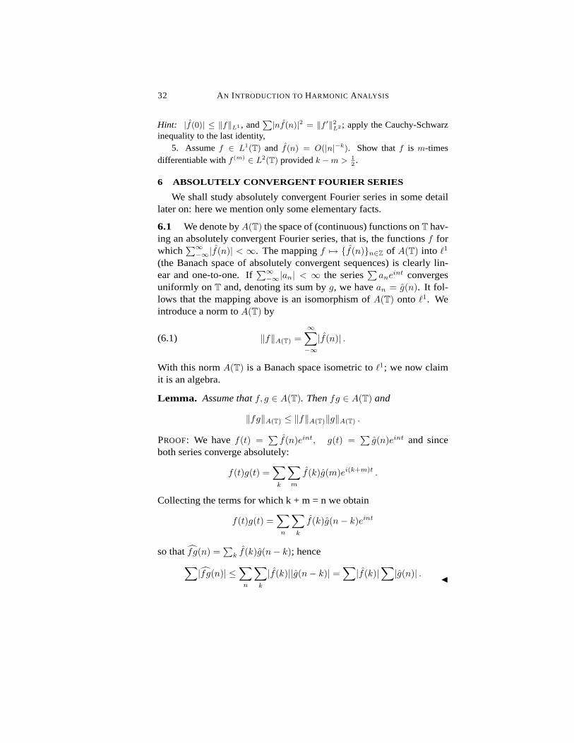
6 ABSOLUTELY CONVERGENT FOURIER SERIES
We shall study absolutely convergent Fourier series in some detaillater on: here we mention only some elementary facts.
6.1 We denote byA(T) the space of (continuous) functions onT hav-ing an absolutely convergent Fourier series, that is, the functionsf forwhich
∑∞−∞|f(n)| < ∞. The mappingf 7→ f(n)n∈Z of A(T) into `1
(the Banach space of absolutely convergent sequences) is clearly lin-ear and one-to-one. If
∑∞−∞|an| < ∞ the series
∑
aneint converges
uniformly onT and, denoting its sum byg, we havean = g(n). It fol-lows that the mapping above is an isomorphism ofA(T) onto `1. Weintroduce a norm toA(T) by
(6.1) ‖f‖A(T) =∞∑
−∞|f(n)| .
With this normA(T) is a Banach space isometric to`1; we now claimit is an algebra.
Lemma. Assume thatf, g ∈ A(T). Thenfg ∈ A(T) and
‖fg‖A(T) ≤ ‖f‖A(T)‖g‖A(T) .
PROOF: We havef(t) =∑
f(n)eint, g(t) =∑
g(n)eint and sinceboth series converge absolutely:
f(t)g(t) =∑
k
∑
m
f(k)g(m)ei(k+m)t .
Collecting the terms for which k + m = n we obtain
f(t)g(t) =∑
n
∑
k
f(k)g(n− k)eint
so thatfg(n) =∑
k f(k)g(n− k); hence∑
|fg(n)| ≤∑
n
∑
k
|f(k)||g(n− k)| =∑
|f(k)|∑
|g(n)| .J

I. FOURIER SERIES ONT 33
6.2 Not every continuous function onT has an absolutely convergentFourier series, and those that have cannot† be characterized by smooth-ness conditions (see exercise 5 of this section). Some smoothness con-ditions are sufficient, however, to imply the absolute convergence ofthe Fourier series.
Theorem. Let f be absolutely continuous onT andf ′ ∈ L2(T). Thenf ∈ A(T) and
(6.2) ‖f‖A(T) ≤ ‖f‖L1 +(
2∞∑
1
n−2) 1
2 ‖f ′‖L2 .
PROOF: This is exercise 4 of the previous section and the hint giventhere is essentially the whole proof. J
?6.3 We refer to exercise 2.2 for the definitions of Lipα(T) and of itsnorm.
Theorem (Bernstein). If f ∈ Lipα(T) for someα > 12 , thenf ∈ A(T)
and
(6.3) ‖f‖A(T) ≤ cα‖f‖Lipα
where the constantcα depends only onα.
PROOF:f(t− h)− f(t) ∼
∑
(e−inh − 1)f(n)eint.
if take h = 2π/(3 ·2m) and2m ≤ n ≤ 2m+1 we have|e−inh − 1| ≥√
3and consequently
∑
2m≤n<2m+1
|f(n)|2 ≤∑
n
|e−inh − 1|2|f(n)|2 = ‖fh − f‖2L2 ≤
≤ ‖fh − f‖2∞ ≤( 2π
3·2m)2α
‖f‖2Lip α .
(6.4)
Noticing that the sum on the left of (6.4) consists of at most2m+1 terms,we obtain by the Cauchy-Schwarz inequality
(6.5)∑
2m≤n<2m+1
|f(n)| ≤ 2(m+1)/2( 2π
3·2m)α
‖f‖Lip α .
Sinceα > 12 , we can sum the inequalities (6.5) form = 0, 1, . . . , and
remembering that|f(0)| ≤ ‖f‖Lipα we obtain (6.3). J
†See, however, exercise 7.8.
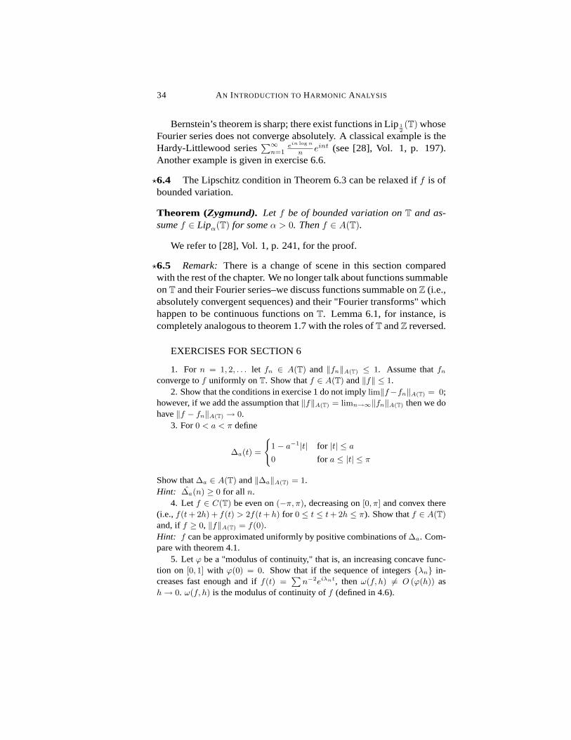
34 AN INTRODUCTION TOHARMONIC ANALYSIS
Bernstein’s theorem is sharp; there exist functions in Lip12(T) whose
Fourier series does not converge absolutely. A classical example is theHardy-Littlewood series
∑∞n=1
ein logn
n eint (see [28], Vol. 1, p. 197).Another example is given in exercise 6.6.
?6.4 The Lipschitz condition in Theorem 6.3 can be relaxed iff is ofbounded variation.
Theorem (Zygmund). Let f be of bounded variation onT and as-sumef ∈ Lipα(T) for someα > 0. Thenf ∈ A(T).
We refer to [28], Vol. 1, p. 241, for the proof.
?6.5 Remark: There is a change of scene in this section comparedwith the rest of the chapter. We no longer talk about functions summableonT and their Fourier series–we discuss functions summable onZ (i.e.,absolutely convergent sequences) and their "Fourier transforms" whichhappen to be continuous functions onT. Lemma 6.1, for instance, iscompletely analogous to theorem 1.7 with the roles ofT andZ reversed.
EXERCISES FOR SECTION 6
1. For n = 1, 2, . . . let fn ∈ A(T) and ‖fn‖A(T) ≤ 1. Assume thatfnconverge tof uniformly onT. Show thatf ∈ A(T) and‖f‖ ≤ 1.
2. Show that the conditions in exercise 1 do not implylim‖f−fn‖A(T) = 0;however, if we add the assumption that‖f‖A(T) = limn→∞‖fn‖A(T) then we dohave‖f − fn‖A(T) → 0.
3. For0 < a < π define
∆a(t) =
1− a−1|t| for |t| ≤ a0 for a ≤ |t| ≤ π
Show that∆a ∈ A(T) and‖∆a‖A(T) = 1.Hint: ∆a(n) ≥ 0 for all n.
4. Letf ∈ C(T) be even on(−π, π), decreasing on[0, π] and convex there(i.e.,f(t+ 2h) + f(t) > 2f(t+ h) for 0 ≤ t ≤ t+ 2h ≤ π). Show thatf ∈ A(T)
and, iff ≥ 0, ‖f‖A(T) = f(0).Hint: f can be approximated uniformly by positive combinations of∆a. Com-pare with theorem 4.1.
5. Letϕ be a "modulus of continuity," that is, an increasing concave func-tion on [0, 1] with ϕ(0) = 0. Show that if the sequence of integersλn in-creases fast enough and iff(t) =
∑
n−2eiλnt, thenω(f, h) 6= O (ϕ(h)) ash→ 0. ω(f, h) is the modulus of continuity off (defined in 4.6).

I. FOURIER SERIES ONT 35
6. (Rudin, Shapiro.) We define the trigonometric polynomialsPm andQminductively as follows:P0 = Q0 = 1 and
Pm+1(t) = Pm(t) + ei2mttQm(t)
Qm+1(t) = Pm(t)− ei2mttQm(t).
(a) Show that
|Pm+1(t)|2 + |Qm+1(t)|2 = 2(
|Pm(t)|2 + |Qm(t)|2)
hence |Pm(t)|2 + |Qm(t)|2 = 2m+1
and ‖Pm‖C(T) ≤ 2(m+1)/2 .
(b) For|n| < 2m, Pm+1(n) = Pm(n), hence there exists a sequenceεn∞n=0
such thatεn is either 1 or -1 and such thatPm(t) =∑2m−1
0εne
int.
(c) Write fm = Pm − Pm+1 = ei2m−1tQm−1 andf =
∑∞1
2−mfm. Showthatf ∈ Lip 1
2(T) andf 6∈ A(T).
Hint: For 2−k ≤ h ≤ 21−k write
f(t+ h)− f(t) =(
k∑
1
+
∞∑
k+1
)
2−m(fm(t+ h)− fm(t)) .
By part (a) the sum∑∞
k+1is bounded by2
∑∞k+1
2−m2m/2 < 5h12 . Using part
(a), exercise 2.12, and the fact thatfm is a trigonometric polyomial of degree2m − 1, one obtains a similar estimate for
∑k
1.
7. Letf, g ∈ L2(T). Show thatf ∗ g ∈ A(T).
7 FOURIER COEFFICIENTS OF LINEAR FUNCTIONALS
We consider a homogeneous Banach spaceB onT and assume, forsimplicity, thateint ∈ B for all n. As usual, we denote byB∗ the dualspace ofB.
7.1 The Fourier coefficients of a functionalµ ∈ B∗ are, by definition:
(7.1) µ(n) = 〈eint, µ〉, n ∈ Z;
and we call the trigonometric series
S[µ] ∼∞∑
−∞µ(n)eint
the Fourier series† of µ. Clearly
|µ(n)| ≤ ‖µ‖B∗‖eint‖B .
†We keep, however, the convention of 1.3 that a Fourier series, without complements,is a Fourier series of a summable function.

36 AN INTRODUCTION TOHARMONIC ANALYSIS
The notation (7.1) is consistent with our definition of Fourier coeffi-cients in case thatµ is identified naturally with a summable function.For instance, ifB = Lp(T), 1 < p < ∞, B∗ is canonically identifiedwith Lq(T) whereq = p/(p− 1). To the functiong ∈ Lq(T) correspondsthe linear functional
f 7→ 〈f, g〉 =1
2π
∫
f(t)g(t)dt, f ∈ Lp(T)
and〈eint, g〉 =
12π
∫
eintg(t)dt =1
2π
∫
e−intg(t)dt
thus g(n) defined in (7.1) for the functionalg coincides with thenthFourier coefficient of the functiong.
Theorem (Parseval’s formula).Let f ∈ B, µ ∈ B∗; then
(7.2) 〈f, µ〉 = limN→∞
N∑
−N
(
1− |n|N + 1
)
f(n)µ(n).
PROOF: (a) For polynomialsP (t) =∑N−N P (n)eint we clearly have
〈P, µ〉 =∑N−N P (n)µ(n).
(b) Since, by theorem 2.11,f = limN→∞ σN (f) in theB norm, itfollows from (a) and the continuity ofµ that
〈f, µ〉 = lim〈σN (f), µ〉 = limN→∞
N∑
−N
(
1− |n|N + 1
)
f(n)µ(n).J
Remark: The fact that the limit in (7.2) exists is an implicit part ofthe theorem. It is equivalent to the C-1 summability‡ of the series∑
f(n)µ(n). If this last series converges then clearly
(7.3) 〈f, µ〉 =∞∑
−∞f(n)µ(n)
We shall sometimes refer to (7.3) as Parseval’s formula, keeping inmind that if the series on the right does not converge then (7.3) is simplyan abbreviation for (7.2).
Corollary ( Uniqueness theorem).If µ(n) = 0 for all n, thenµ = 0.
‡Cesàro of order 1

I. FOURIER SERIES ONT 37
7.2 We shall writeµ ∼∑
µ(n)eint, and may writeµ =∑
µ(n)eint
if the series converges in some sense (which should be clear from thecontext). This is an abuse of language which, if used with caution,presents no risk of misunderstanding and obviates tedious repetitions.
In accordance with our abuse of language we define, forµ ∈ B∗, theelementsSn(µ) andσn(µ) of B∗ by
Sn(µ) =n∑
−nµ(j)eijt
σn(µ) =n∑
−n
(
1− |j|n+ 1
)
µ(j)eijt(7.4)
We shall also write
Sn(µ, t) =n∑
−nµ(j)eijt
σn(µ, t) =n∑
−n
(
1− |j|n+ 1
)
µ(j)eijt(7.5)
The correspondence between the functionals (7.4) and the functions(7.5) is clearly
〈f, Sn(µ)〉 =1
2π
∫
f(t)Sn(µ, t)dt =n∑
−nf(j)µ(j)
for all f ∈ B; similarly for σn(µ).The mappingSn : f 7→ Sn(f) on B is clearly a bounded linear
operator, and so isSn : µ 7→ Sn(µ) onB∗. It follows from Parseval’sformula thatSn onB∗ is the adjoint ofSn onB and consequently hasthe same norm. Similarly,σn : µ 7→ σn(µ) on B∗ is the adjoint ofσn : f 7→ σn(f) on B and consequently§ ‖σn‖B
∗= 1.
We remark that by Parseval’s formula, for everyµ ∈ B∗, σn(µ)converges weak-star toµ.
7.3 Parseval’s formula enables us to characterize sequences of Fouriercoefficients of linear functionals.
Theorem. LetB be a homogeneous Banach space onT. Assume thateint ∈ B for all n. Let an∞n=−∞ be a sequence of complex numbers.Then the following two conditions are equivalent:
§‖σn‖B∗
denotes the norm ofσn as operator onB∗.

38 AN INTRODUCTION TOHARMONIC ANALYSIS
(a) There existsµ ∈ B∗, ‖µ‖ ≤ C, such thatµ(n) = an for all n.(b) For all trigonometric polynomialsP
∣
∣
∑
P (n)an∣
∣ ≤ C‖P‖B .
PROOF: The implication (a)⇒ (b) follows immediately from Parse-val’s formula. If we assume (b) then
(7.6) P 7→∑
P (n)an
is a linear functional on the space of all trigonometric polynomials,bounded in the B norm, and therefore (theorem 2.12) admits a uniqueextensionµ of norm< C toB. Sinceµ extends (7.6) we have
µ(n) = 〈eint, µ〉 = an. J
Corollary. A trigonometric seriesS ∼∑
aneint is the Fourier series
of someµ ∈ B∗, ‖µ‖ ≤ C, if, and only if, ‖σN (S)‖ ≤ C for all N .Here σN (S) denotes the element in B* the Fourier series of which is∑NN (1− |j|/(N + 1))ajeijt.
PROOF: The necessity follows from 7.2; the sufficiency from the cur-rent theorem and the observation that for trigonometric polynomialsP
∑
P (n)an = limN→∞
〈P, σN (S)〉 .J
7.4 In the caseB = C(T ) the dual spaceB∗ is identified with thespaceM(T) of all (Borel) measures onT (we set〈f, µ〉 =
∫
fdµ) Weshall refer to Fourier coefficients of measures as Fourier-Stieltjes co-efficients and to Fourier series of measures as Fourier-Stieltjes series.The mappingf 7→ (1/2π)f(t)dt is an isometric embedding ofL1(T)in M(T). The Fourier coefficients of(1/2π)f(t)dt are preciselyf(n),hence a Fourier series is a Fourier-Stieltjes series.
An example of a measure that is not obtained as(1/2π)f(t)dt is theso-called Dirac measure; it is the measureδ of mass one concentratedat t = 0. δ can also be defined by〈f, δ〉 = f(0) for all f ∈ C(T). Wedenote byδτ , τ ∈ T, the unit mass concentrated atτ . Thusδ = δ0 and〈f, δτ 〉 = f(τ) for all τ ∈ T. From (7.1) it follows thatδτ (n) = e−inτ
and in particularδ(n) = 1. This shows that Fourier-Stieltjes coefficientsneed not tend to zero at infinity (however, by 7.1,|µ(n)| ≤ ‖µ‖M(T)).

I. FOURIER SERIES ONT 39
7.5 We recall that a measureµ is positive ifµ(E) ≥ 0 for every mea-surable setE, or equivalently, if
∫
fdµ ≥ 0 wheneverf ∈ C(T) is non-negative. Ifµ is absolutely continuous, that is, ifµ = (1/2π)g(t)dt withg ∈ L1(T), thenµ is positive if and only ifg(t) ≥ 0 almost everywhere.
Lemma. A seriesS ∼∑
aneint is the Fourier-Stieltjes series of a
positive measure if, and only if, for alln andt ∈ T,
σn(S, t) =n∑
−n
(
1− |j|/(n+ 1))
ajeijt ≥ 0.
PROOF: If S = S(µ) for a positiveµ ∈ M(T) and if f ∈ C(T) is non-negative, we have
12π
∫
f(t)σn(S, t)dt =n∑
−n
(
1− |j|n+ 1
)
f(j)µ(j) = σn(f)dµ ≥ 0
sinceµ ≥ 0 and, by 3.1,σn(f, t) > 0. Since this is true for arbitrarynonnegativef , σn(S, t) ≥ 0 onT. Assumingσn(S, t) ≥ 0 we obtain
‖σn(S)‖M(T) =1
2π
∫
σn(S, t)dt = a0
and, by Corollary 7.3,S = S(µ) for someµ ∈ M(T). For arbitrarynonnegativef ∈ C(T),
∫
fdµ = limn→∞(l/2π∫
f(t)σn(S, t)dt ≥ 0 andit follows thatµ is a positive measure. J
Remark: The condition “σn(S, t) ≥ 0 for all n” can clearly be replacedby “σn(S, t) ≥ 0 for infinitely manyn’s”.
7.6 We are now able to characterize Fourier-Stieltjes coefficients ofpositive measures as positive definite sequences.
DEFINITION: A numerical sequenceann∈Z is positive definite if forany sequencezn having only a finite number of terms different fromzero we have
(7.7)∑
n,m
an−mznzm ≥ 0.
Theorem (Herglotz). A numerical sequenceann∈Z is positive def-inite if, and only if, there exists a positive measureµ ∈ M(T) such thatan = µ(n) for all n.

40 AN INTRODUCTION TOHARMONIC ANALYSIS
PROOF: Assumean = µ(n) with positiveµ. Then
(7.8)∑
n,m
an−mznzm =∑
n,m
∫
e−inteimtznzm =∫∣
∣
∣
∑
n
zne−int
∣
∣
∣
2
dµ ≥ 0.
If, on the other hand, we assume thatan is positive definite, we writeS ∼
∑
aneint and, for arbitraryN andt ∈ T we choose
zn =
eint |n| ≤ N0 |n| > N
We have∑
n,m an−mznzm =∑
j Cj,Najeijt whereCj,N is the number
of ways to writej in the formn −m where|n| ≤ N and|m| ≤ N , thatis,Cj,N = max(0, 2N + 1− |j|). It follows that
σ2N (S, t) =1
2N + 1
∑
j
Cj,Najeijt ≥ 0
and the theorem follows from 7.5. J
7.7 If an is positive definite, then
(7.9) |an| ≤ a0,
and the sequence(an − an−1+an+12 ) is positive definite. This can be
seen directly by checking condition (7.7), or deduced from Herglotz’theorem and the observations that ifµ is the positive measure such thatan = µ(n), thena0 = µ(0) = ‖µ‖, ν = (1 − cos t)µ is nonnegative, andν(n) = an − an−1+an+1
2 .Also, sincean = a−n, we havea0 −<a1 = a0 − a−1+a1
2 = ν(0).Combining all this, we obtain
Lemma. If an is positive definite, then
(7.10)∣
∣
∣
(
an −an−1 + an+1
2)
∣
∣
∣ ≤ a0 −<a1.
Positive definite functions can be defined over any abelian group bythe same inequality (7.7). In Chapter VI we shall see that the precedinglemma implies in particular that positive definite functions onR thatare continuous at0 are in fact uniformly continuous.

I. FOURIER SERIES ONT 41
7.8 The Spectral Theorem.Positive definite sequences arise nat-urally in the context of unitary operators on a Hilbert space. LetHbe a Hilbert space,U a unitary operator onH, and f ∈ H; writean = 〈U−nf, f〉. The sequencean is positive definite since for anyfinite sequencezn we have
∑
n,m
an−mznzm =∑
n,m
〈znU−nf, zmU−mf〉
=∥
∥
∥
∑
n
znU−nf
∥
∥
∥
2
H≥ 0.
(7.11)
The positive measureµ = µf ∈M(T) for which µ(n) = an is calledthespectral measure off . Comparing (7.8) and (7.11), one realizes thatthe correspondence
(7.12) H 3 Unf ←→ eint ∈ L2(µf )
extends to an isometry of the closed spanHf of Unf in H ontoL2(µf ), which conjugatesU to the operator of multiplication byeit onL2(µf ). This is in essence¶ the spectral theorem for unitary operatorson a Hilbert space.
Corollary ( The Ergodic Theorem).LetH be a Hilbert space andU a unitary operator onH. Denote byHinv the subspace ofU-invariantvectors inH, and byPinv the orthogonal projection ofH onHinv. Then
lim1N
N−1∑
0
U j = Pinv,
the limit in the strong operator topology.
PROOF: The claim is that for everyf ∈ H, lim 1N
∑N−10 U jf = Pinvf in
norm. By the spectral theorem, we may assume thatU is multiplicationby eit onL2(µf ), and so1
N
∑N−10 U j is just multiplication by
ϕN (t) =1N
N−1∑
0
eijt =eiNt − 1N(eit − 1)
.
The elements ofL2(µf ) which are invariant under multiplication byeit are just the multiples of110 (the indicator function of0), and
¶What we omit here is the analysis of themultiplicity of U onH.

42 AN INTRODUCTION TOHARMONIC ANALYSIS
Pinv in this context is multiplication by110. As ‖ϕN‖∞ = 1 andϕNconverge pointwise to110, we havelimϕNψ = ψ(0)110 in norm foranyψ ∈ L2(µf ), and in particular for the constant 1, the image off
under the “spectral” isometry. J
7.9 An important property of Fourier-Stieltjes coeffcients is that ofbeing "universal multipliers." More precisely:
Theorem. LetB be a homogeneous Banach space onT andµ ∈M(T).There exists a unique linear operatorµ onB having the following prop-erties:(i) ‖µ‖ ≤ ‖µ‖M(T)
(ii) µf(n) = µ(n)f(n) for all f ∈ B.
PROOF: If an operatorµ satisfies (ii), then forf =∑n−N f(n)eint we
haveµf =∑N−N µ(n)f(n)eint, that is,µ is completely determined on
the polynomials inB. If µ is bounded it is completely determined. Inorder to show the existence ofµ it is suffcient to show that if we define
(7.13) µf =∑
µ(n)f(n)eint
for all polynomialsf then
(7.14) ‖µf‖ ≤ ‖µ‖M(T)‖f‖B ,
sinceµ would then have a unique extension of norm≤ ‖µ‖M(T) to allof B. If µ = (1/2π)g(t)dt with g ∈ C(T), it is clear thatµf , as definedin (7.13), is simplyg ∗ f which we can write as aB-valued integral (see2.4)
(7.15) µf = g ∗ f =1
2π
∫
g(τ)fτdτ
and deduce the estimate
‖µf‖B ≤ ‖f‖B ·1
2π
∫
|g(τ)|dτ = ‖µ‖M(T)‖f‖B .
For arbitraryµ ∈ M(T), σn(µ) has the form(1/2π)gn(t)dt, wheregn(t) =
∑n−n(1− |j|/(n+ 1))µ(j)eijt and
12π
∫
|gn(t)|dt = ‖σn(µ)‖M(T) ≤ ‖µ‖M(T) .
By our previous remark‖gn∗f‖B ≤ ‖µ‖M(T)‖f‖B. Sincef is a trigono-metric polynomial, we clearly haveµf = limn→∞ gn ∗ f and (7.14)follows. J

I. FOURIER SERIES ONT 43
Corollary. Letf ∈ B andµ ∈M(T). Thenµ(n)f(n) is the sequenceof Fourier coefficients of some function inB.
In view of (7.15) we shall writeµ ∗ f instead ofµf , and refer to it asthe convolution ofµ andf . With this notation, our earlier condition (ii)becomes a (formal) extension of (1.10).
7.10 Forµ ∈M(T) we defineµ# ∈M(T) by
(7.16) µ#(E) = µ(−E)
for every Borel setE (recall that−E = t : − t ∈ E), or equivalently,by
(7.17)∫
f(t)dµ# =∫
f(−t)dµ
for all f ∈ C(T). It follows from (7.17) that
(7.18) µ#(n) = µ(n) .
7.11 By Parseval’s formula, the adjoint ofµ is the operator whichassigns to everyν ∈ B∗ the element ofB∗ whose Fourier series is givenby∑
µ(n)ν(n)eint =∑
µ#(n)ν(n)eint. We extend the notation of 7.7,write this element ofB∗ asµ# ∗ ν, and refer to it as the convolution ofµ# andν. We summarize:
Theorem. Let B be a homogeneous Banach space onT andB∗ itsdual. Letµ ∈M(T), ν ∈ B∗; then
∑
µ(n)ν(n)eint is the Fourier seriesof an elementµ ∗ ν ∈ B∗. Moreover‖µ ∗ ν‖B∗ ≤ ‖µ‖M(T)‖ν‖B∗ .
The norm estimate follows from (7.14) and the facts that the normof the adjoint of an operator is equal to the norm of the operator, and‖µ#‖M(T) = ‖µ‖M(T) .
It follows, in particular, that ifµ, ν ∈M(T), then∑
µ(n)ν(n)eint isthe Fourier-Stieltjes series of the measureµ ∗ ν.
7.12 We have introduced the convolution ofµ, ν ∈ M(T) by itsFourier-Stieltjes series. It can, of course, be done directly. Withµ
andν given, and forf ∈ C(T), the double integral
I(f) =∫∫
f(t+ τ)dµ(t)dν(τ)

44 AN INTRODUCTION TOHARMONIC ANALYSIS
is well defined, is clearly linear inf , and satisfies
|I(f)| ≤ ‖µ‖M(T)‖ν‖M(T).
By the Riesz representation theorem, which identifiesM(T) as the dualof C(T), there exists a measureλ ∈ M(T) such thatI(f) =
∫
f(t)dλ.Takingf(t) = e−int we obtainλ(n) = µ(n)ν(n), that is,λ = µ ∗ ν. Inother words
(7.19)∫
fd(µ ∗ ν) =∫∫
f(t+ τ)dµ(t)dν(τ) .
Taking a (bounded) sequence of functionsf which converge to the in-dicator function of an arbitrary closed setE, we see that (7.19) is equiv-alent to (denotingE − τ = t : t+ τ ∈ E)
(7.20) (µ ∗ ν)(E) =∫
µ(E − τ)dν(τ) .
By regularity, (7.20) holds for every Borel setE.
7.13 We recall that a measureµ ∈ M(T) is discrete ifµ =∑
ajδτjwhereaj are complex numbers; we then have‖µ‖M(T) =
∑
|aj |. Ameasureµ is continuous ifµ(t) = 0 for every t ∈ T (t is the setwhose only member is the pointt). Equivalentlyµ is continuous iflimη→0
∫ t+η
t−η |dµ| = 0 for all t ∈ T. Everyµ ∈ M(T) can be uniquelydecomposed to a sumµ = µc + µd whereµc is continuous andµd isdiscrete.
It is clear from (7.20) that ifµ is a continuous measure then, foreveryν ∈M(T), µ∗ν is continuous. Also, sinceδ(τ)∗δ(τ ′) = δ(τ +τ ′),if µ =
∑
ajδτj , and ν =∑
bkδτ ′k
thenµ ∗ ν =∑
j,k ajbkδτj+τ ′k . Ifµ = µc + µd is the decomposition ofµ into continuous and discreteparts, thenµ#
c the continuous part ofµ# andµ#d is its discrete part.
Thusµ ∗ µ# = (µc ∗ µ#
c + µc ∗ µ#d + µd ∗ µ#
c ) + µd ∗ µ#d ,
the sum of the first three terms is continuous and the last term is dis-crete. Ifµd =
∑
ajδτj thenµ#d =
∑
ajδ−τj and consequently the massat τ = 0 of the measureµ ∗ µ# is
∑
|aj |2. We have proved:
Lemma. Let µ ∈ M(T). Then∑
|µ(τ)|2 = (µ ∗ µ#)(0). Inparticular: µ is continuous if, and only if,
(µ ∗ µ#)(0) = 0.

I. FOURIER SERIES ONT 45
The discrete part of a measureµ can be “recovered” from its Fourier-Stieltjes series.
Theorem. Letµ ∈M(T), τ ∈ T. Then
µ(τ) = limN→∞
12N + 1
N∑
−N
µ(n)einτ .
PROOF: The functionsϕN (t) = 12N+1DN (t−τ) = 1
2N+1
∑N−N e
−inτeint
are bounded by 1 and tend to zero uniformly outside any neighborhoodof t = τ . Remembering that
limϑ→0
∫ τ+ϑ
τ−ϑ|d(µ− µ(τ)δτ )| = 0
we obtain
(7.21) limN→∞
〈ϕN , µ− µ(τ)δτ 〉 = 0
Now
〈ϕN , µ− µ(τ)δτ 〉 =1
2N + 1
N∑
−N
µ(n)einτ − µ(τ)
and the theorem follows from (7.21). J
Corollary ( Wiener). Letµ ∈M(T). Then
(7.22)∑
|µ(τ)|2 = limN→∞
12N + 1
N∑
−N
|µ(n)|2 .
In particular: µ is continuous if, and only if,
(7.23) limN→∞
12N + 1
N∑
−N
|µ(n)|2 = 0.
Remarks:a. The averaging that appears in the Theorem and in thecorollary need not be on intervals symmetric with respect to 0. IfMjis an arbitrary sequence of integers, andNj →∞, then for allτ ∈ T
(7.24) µ(τ) = limj→∞
1Nj + 1
Mj+Nj∑
Mj
µ(n)einτ .

46 AN INTRODUCTION TOHARMONIC ANALYSIS
The proof as above, withϕN replaced byΦj = 1Nj+1
∑Mj+NjMj
eint .
b. The exponent 2 in (7.22) is essential, in (7.23) it can be re-placed by any positive number. What the condition really says is thatµ(n) tends to zero in density, that is: givenε > 0, the proportion in allsufficiently large intervals, of the integersn such that|µ(n)| > ε, is ar-bitrarily small. In particular, for everyε > 0 and positiveN there existin any sufficiently large interval onZ, intervals of lengthN , on which|µ| < ε.
EXERCISES FOR SECTION 7
1. LetB be homogeneous onT andB∗ its dual. Show thatS ∼∑
aneint
is the Fourier series of someµ ∈ B∗ if and only if ‖σN (S)‖ is bounded asN →∞.
2. DenoteKn,τ (t) = KN (t− τ). Show that for everyµ ∈M(T)
σn(µ, τ) = 〈Kn,τ , µ〉 .
Deduce thatσn(µ, τ) ≥ 0 if µ is positive.3. Show that a trigonometric series
∑
aneint such that
∑N
−N aneint ≥ 0
for all N andt ∈ T is a Fourier-Stieltjes series of a positive measure.4. We shall prove later (see IV.2.1) that iff ∈ Lp(T) with 1 < p ≤ 2, then
‖f‖`q =(∑
|f(n)|q)1/q
≤ ‖f‖Lp(T)
(
q =p
p− 1
)
, .
Assuming this, show that ifan ∈ `p is a numerical sequence then there existsa functiong ∈ Lq(T) such thatg(n) = an, and‖g‖Lq(T) ≤ ‖an‖`p .
5. The elements of the dual space ofCm(T) are calleddistributions oforderm onT. We denote byDm(T) = (Cm(T))∗ the space of distributions oforderm on T. SinceCm+1(T) ⊂ Cm(T) we haveDm(T) ⊂ Dm+1(T). WriteD(T) = ∪mDm(T).
(a) Prove that ifµ ∈ Dm then
|µ(n)| ≤ const |n|m n 6= 0.
(b) Given a numerical sequencean satisfyingan = O (|n|m), there exists adistributionµ ∈ Dm+1 such thatan = µ(n) for all n.
Hint: If f ∈ Cm+1(T) then∑
|nmf(n)| <∞.
Thus a trigonometric series∑
aneint is the Fourier series of a distribution
onT if and only if, for somem, an = O (|n|m) n 6= 0.
Let µ ∈ D and letO be an open subset ofT. We say thatµ vanishes onOif 〈ϕ, µ〉 = 0 for all ϕ ∈ C∞(T) such that the support ofϕ (i.e., the closureof the sett :ϕ(t) 6= 0) is contained inO.

I. FOURIER SERIES ONT 47
(c) Prove that ifµ vanishes on the open setsO1 andO2, then it vanishes onO1 ∪O2.
Hint: Show that if the support ofϕ ∈ C∞(T) is contained inO1 ∪ O2
then there existϕ1, ϕ2 ∈ C∞(T), with supports contained inO1, O2 re-spectively, such thatϕ = ϕ1 + ϕ2.
(d) Extend the result of (c) to any finite union of open sets; hence, using thecompactness of the support of the test functionsϕ, show that ifµ vanishesin the open setsOα, α running over some index setI, thenµ vanishess on⋃
α∈I Oα.
Thus the union of all the open subsets ofT on whichµ vanishes is againsuch a set. This is clearly the largest open set on whichµ vanishes.
DEFINITION: Thesupportof µ is the complement inT of the largest opensetO ⊂ T on whichµ vanishes.
(e) Show that ifµ ∈ Dm and if f ∈ Cm(T) vanishes on a neighborhood ofthe support ofµ, then〈f, µ〉 = 0. The same conclusion holds if for somehomogeneous Banach spaceB, the distributionµ belongs toB∗ andf ∈ B(see exercise 2.11).
(f) We define the derivativeµ′ of a distributionµ ∈ Dm by
〈f, µ′〉 = −〈f ′, µ〉 for f ∈ Cm+1(T).
Show thatµ′ ∈ Dm+1 andµ′(n) = in µ(n).
(g) Show thatsupport(µ′) ⊂ support(µ).
(h) Show that the mapµ 7→ µ′ mapsDm onto the subspace ofDm+1 consistingof all µ ∈ Dm+1 satisfyingµ(0) = 0.
Hence, everyµ ∈ Dm can be written in the formµ(0)dt + µ1 whereµ1 isthemth derivative of a measure.
(i) A distribution µ on T is positiveif 〈f, µ〉 ≥ 0 for every nonnegative testfunctionf ∈ C∞(T). Show that a positive distribution is a measure.
Hint: Positivity implies, for real-valuedf , 〈f, µ〉 ≤ max f(t)〈1, µ〉.6. The dual space ofA(T) is commonly denoted byPM(T) and its ele-
ments referred to as pseudo-measures. Show that with the natural identifica-tionsM(T) ⊂ PM(T) ⊂ D1(T), andPM(T) consists precisely of thoseµ forwhich µ(n) is bounded. Moreover, the correspondenceµ ↔ µ(n) is anisometry ofPM(T) onto`∞.
7. Letα, β ∈ T, letN be an integer, and letµ be the measure carried by thearithmetic progressionα+ jβNj=−N , which places the mass zero atα and themassj−1 atα+ jβ, 1 ≤ |j| ≤ N . Show that‖µ‖PM(T) ≤ π + 2.Hint: See exercise 3.4.
8. Letf ∈ A(T) be real valued and monotonic in a neighborhood oft0 ∈ T.Show that|f(t)− f(t0)| = O
(
(log|t− t0|−1)−1)
ast→ t0.

48 AN INTRODUCTION TOHARMONIC ANALYSIS
9. Let µ, µn ∈ M(T), n = 1, 2, . . . . Prove thatµn → µ in the weak-startopology if, and only if,‖µn‖M(T) = O (1) andµn(j)→ µ(j) for all j.
10. By definition, a sequenceξn∞n=1 ⊂ T is uniformly distributedif forany arcI ⊂ T we havelimN→∞N
−1∑N
n=111I(ξn) = (2π)−1|I|. Prove the
following statements:a. ξn∞n=1 ⊂ T is uniformly distributed if, and only if,µn = n−1
∑n
1δξj
converge in the weak-star topology to(2π)−1dt, i.e., if for all integersl 6= 0,n−1
∑n
1eilξj → 0. (Weyl’s criterion).
b. if α is an irrational multiple ofπ, the sequencenα is uniformly distributedonT.
11. Show that a measureµ ∈M(T) is absolutely continuous if, and only if,limτ→0‖µτ − µ‖ = 0, whereµτ is the translate ofµ by τ (defined byµτ (E) =
µ(E − τ)).12. Letµ ∈M(T). Prove:σn(µ, t) converge to zero at everyt 6∈ support(µ),
the convergence uniform on every closed set disjoint from support(µ).13. Letµ ∈M(T) be singular with respect to dt (that is, there exists a Borel
setE0 of Lebesgue measure zero, such thatµ(E) = µ(E ∩ E0) for every BorelsetE). Show thatσn(µ, t)→ 0 almost everywhere (dt).
14. Show that the conclusion of exercise 12 is false if we assumeµ ∈ D1
instead ofµ ∈ M(T); however, if we replace Fejér’s kernel by Poisson’s, theconclusion is valid for everyµ ∈ D.Hint: For 0 < δ < π, and positive integersm, limr→1
∂mP(r,t)∂tm
= 0 uniformlyin (δ, 2π − δ).
15. (Bernstein’s inequality)Let tj,n = (2j+1)π4n
, andδj,n = δtj,n . Write
µn =1
2n
2n−1∑
0
δj,n, νn = Kn(t)µn.
(a) Check that‖νn‖ = νn(0) = 1.
(b) Writeν∗n = neintνn, then‖ν∗n‖ = n, and ν∗n(j) is periodic of period4n and
ν∗n(j) =
j for |j| ≤ n,2n− j for n ≤ j ≤ 3n.
(c) Prove Bernstein’s inequality:if P =∑n
−n ajeijt, then
(7.25) ‖P ′‖∞ ≤ n ‖P‖∞ .
Hint: P ′ = ν∗n ∗ P .
(d) Prove that ifP =∑n
−n ajeijt, then ‖˜P ′‖∞ ≤ n ‖P‖∞ .
Hint: Find a measureµn of normn such thatµn(j) = |j| for |j| ≤ n.
(e) LetB be a homogeneous Banach space onT, andP =∑n
−n ajeijt ∈ B.
Prove that‖P ′‖B ≤ n‖P‖B, and‖˜P ′‖B ≤ n ‖P‖B .
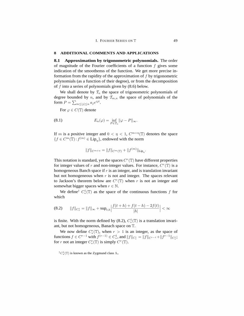
I. FOURIER SERIES ONT 49
8 ADDITIONAL COMMENTS AND APPLICATIONS
8.1 Approximation by trigonometric polynomials. The orderof magnitude of the Fourier coefficients of a functionf gives someindication of the smoothenss of the function. We get more precise in-formation from the rapidity of the approximation off by trigonometricpolynomials (as a function of their degree), or from the decompositionof f into a series of polynomials given by (8.6) below.
We shall denote byTn the space of trigonometric polynomials ofdegree bounded byn, and byTm,n the space of polynomials of theform P =
∑
m≤|j|≤n ajeijt.
Forϕ ∈ C(T) denote
(8.1) En(ϕ) = infP∈Tn
‖ϕ− P‖∞.
If m is a positive integer and0 < η < 1, Cm+η(T) denotes the spacef ∈ Cm(T) : f (m) ∈ Lipη, endowed with the norm
‖f‖Cm+η = ‖f‖Cm(T) + ‖f (m)‖Lipη .
This notation is standard, yet the spacesCr(T) have different propertiesfor integer values ofr and non-integer values. For instance,Cr(T) is ahomogeneous Banch space ifr is an integer, and is translation invariantbut not homogeneous whenr is not and integer. The spaces relevantto Jackson’s theorem below areCr(T) when r is not an integer andsomewhat bigger spaces whenr ∈ N.
We define† C1∗(T) as the space of the continuous functionsf for
which
(8.2) ‖f‖C1∗
= ‖f‖∞ + supt,h∣
∣
∣
f(t+ h) + f(t− h)− 2f(t)|h|
∣
∣
∣ <∞
is finite. With the norm defined by (8.2),C1∗(T) is a translation invari-
ant, but not homogeneous, Banach space onT.We now defineCr∗(T), whenr > 1 is an integer, as the space of
functionsf ∈ Cr−1 with f (r−1) ∈ C1∗ , and‖f‖Cr∗ = ‖f‖Cr−1 +‖fr−1‖C1
∗;
for r not an integerCr∗(T) is simplyCr(T).
†C1∗(T) is known as the Zygmund classΛ∗

50 AN INTRODUCTION TOHARMONIC ANALYSIS
8.2 Jackson’s theorem is the direct part of the following
Theorem. Let r > 0. If f ∈ Cr∗(T), then:
(8.3) En(f) = O(
n−r)
.
Conversely,(8.3) impliesf ∈ Cr∗(T).
We prove the theorem in a more general context and slightly differ-ent form. We replaceC(T) by any homogeneous Banach spaceB onTand defineEn(f,B) for f ∈ B byEn(f,B) = inf‖f −P‖B, the infimumfor all trigonometric polynomialsP of degree≤ n.
For 0 < r < 1 we defineCr∗(B) akaCr(B) aka Lipr(B) as the setf ∈ B : ‖fh − f‖B = O(|h|r). With the norm
‖f‖Cr∗(B) = ‖f‖B + suph|h|−r‖fh − f‖Bit is a translation invariant Banach space onT.
For r = 1 we set
‖f‖C1∗(B) = ‖f‖B + suph|h|−1‖fh + f−h − 2f‖B
andC1∗(B) the subspace ofB of elementsf with ‖f‖C1
∗finite. Finally,
for r > 1 we writer = m+ η, m an integer and0 < η ≤ 1, define
‖f‖Cr∗(B) = ‖f‖B + ‖f (m)‖Cη∗ (B)
andCr∗(B) the subspace ofB of elementsf with ‖f‖Cr∗ finite.
8.3 The usefulness of the de la Vallée Poussin kernel in this contextbecomes apparent from the following observation‡.
Lemma. AssumeB a homogeneous Banach space onT and f ∈ B.Then
(8.4) E2n+1(f,B) ≤ ‖f − Vn ∗ f‖B ≤ 4En(f,B).
PROOF: The inequality on the left is obvious. For the other inequalitynotice that ifP is a polynomial of degreen, thenVn ∗ P = P , and
‖f − Vn ∗ f‖B =‖(f − P )− Vn ∗ (f − P‖B ≤≤(
1 + ‖Vn‖L1(T)
)
‖f − P‖B < 4‖f − P‖B . J
Forn ≥ 2, we writeWn(f) = (V2n − Vn) ∗ f . With P as above,
(V2n − Vn) ∗ f = (V2n − Vn) ∗ (f − P ),
‡By comparison: forf = cos t andn > 0, En(f) = 0 while σn(f)− f = n−1f .

I. FOURIER SERIES ONT 51
and since‖V2n − Vn‖L1(T) < 3, we obtain
(8.5) ‖Wn(f)‖B ≤ 3En(f,B).
We setW1(f) = V2 ∗ f , and have
(8.6) f = limV2k ∗ f =∑
k≥1
W2k(f).
In particular,f − V2j ∗ f =∑
k≥jW2k(f), so that
(8.7) E2j+1+1(f,B) ≤∑
k≥j
‖W2k(f)‖B .
In view of (8.5) and (8.7) the following is equivalent to Theorem 8.2.
Theorem. LetB be a homogeneous Banach space onT, andr > 0. Anecessary and sufficient condition forf ∈ Cr∗(B) is
(8.8) ‖Wn(f)‖B = O(
n−r)
.
In the proof that (8.8) follows fron the assumptionf ∈ Cr∗(B) weuse Bernstein’s as well as the “reverse inequality”, which are discussedin the next subsection. The converse is proved in the subsection 8.5.
8.4 The “reverse Bernstein inequality”. Bernstein’s inequality,for polynomials of degreen, ‖P ′‖∞ ≤ n‖P‖∞, is outlined in detailin exercise 7.15. The main observation is that for anyn there exists ameasureν∗n such that‖ν∗n‖ = n andν∗n(j) = j for |j| ≤ n.
If P is a polynomial of degreen, thenP ′ = iν∗n ∗ P and hence‖P ′‖B ≤ n‖P‖B for any homogeneous Banach spaceB. Applying thisrepeatedly one has, for any integerm > 0,
(8.9) ‖P (m)‖B ≤ nm‖P‖B .
The “reverse inequality” is proven in a similar way; its statement isthe following theorem.
Theorem. LetB be a homogeneous Banach space onT, andm > 0an integer. There exist a constantCm such that iff =
∑
|j|≥n ajeijt is
in Cm(T) andf (m) ∈ B, thenf ∈ B and
(8.10) ‖f‖B ≤ Cm|n|−m‖f (m)‖B .

52 AN INTRODUCTION TOHARMONIC ANALYSIS
For evenm we obtainCm = m+ 1, for oddm, Cm = 12m will do§.
PROOF: We prove the following statement:given positive integersmandn, there exist measuresµm,n such that
(8.11) ‖µm,n‖M(T) ≤ Cmn−m, and µm,n(j) = j−m for |j| ≥ n.
Sincef = i−mµm,n ∗ f (m), this clearly implies (8.10).Denote byφm,n the positive function inL1(T) whose Fourier coef-
ficients are given by
φm,n(j) =
|j|−m for |j| ≥ nn−m + (n− |j|)(n−m − (n+ 1)−m) for |j| < n.
The coefficients in the range|j| < n are chosen so as to fulfill theconditions of Theorem 4.1: they are symmetric, linear in[0, n+ 1] withslope matching that ofj−m on [n, n+ 1], so thatφm,n(j) is convex on[0,∞). It follows that
‖φm,n‖L1 = φm,n(0) < (m+ 1)n−m.
For evenm setµm,n = φm,ndt and obtainCm = m+ 1.
Form = 1, writeψl =(
e2lit + 12e
3lit)
Kl−1 and Ψn,k = ψn2k−1 .
‖Ψn,k‖L1(T) ≤ 3/2, Ψn,k(j) = 0 for j ≤ 0, and∑∞k=0
Ψn,k(j) = 1for j ≥ n. It follows that the function
Φ∗n(t) =∞∑
k=0
Ψn,k ∗ φ1,n2k
satisfies:Φ∗n(j) = 0 for j ≤ 0, Φ∗n(j) = 1/j for all j ≥ n, and
(8.12)∥
∥
∥Φ∗n∥
∥
∥
L1(T)≤ 3/2
∞∑
k=0
‖φ1,n2k‖ ≤ 6n−1.
We setµ1,n =(
Φ∗n(t)− Φ∗n(−t))
dt, and (8.10) holds withC1 = 12.Finally, form = 2l + 1 we setµm,n = µ1,n ∗ µ2l,n andCm = 12m. J
Remark: If P ∈ Tn,4n, that is has the formP =∑
n≤|j|≤4n ajeijt, then
(8.13) C−1m nm‖P‖B ≤ ‖P (m)‖B ≤ (4n)m‖P‖B .
§Notice that the general case follows, by iteration, from the casem = 1; however theestimate forC(m) obtained this way is exponential rather than linear inm.

I. FOURIER SERIES ONT 53
We turn to the proof that the assumptionf ∈ Cr∗(B) implies (8.8),and begin with the case0 < r ≤ 1. We estimateEn(f) using the JacksonkernelJn(t) = ‖Kn‖−2
L2K2n(t). It is a symmetric summability kernel and,
for −π < t < π, it satisfies
Jn(t) < 2π4n−3t−4.
If f ∈ Cr∗(B) we have
∥
∥
∥Jn ∗ f − f∥
∥
∥
B=∥
∥
∥
12π
∫
Jn(τ)(fτ − f)dτ∥
∥
∥
B
=∥
∥
∥
12π
∫ π
0
Jn(τ)(fτ + f−τ − 2f)dτ∥
∥
∥
B
=∥
∥
∥
12π
(
∫ 1/n
0
+∫ π
1/n
)
Jn(τ)(fτ + f−τ − 2f)dτ∥
∥
∥
B
(8.14)
In [0, 1/n] we have‖fτ + f−τ − 2f‖B = O(n−r). In [1/n, π] we have‖fτ + f−τ − 2f‖B = O(τ r) so that
∥
∥
∥
∫ π
1/n
Jn(τ)(fτ + f−τ − 2f)dτ∥
∥
∥
B≤ Cn−3
∫ π
1/n
τ r−4dτ = O(n−r).
By (8.5) we have‖Wn(f)‖B = O(n−r).If r > 1 we write r = m + η, m an integer and0 < η ≤ 1, and
apply the estimate just obtained tog = f (m). Sinceg ∈ Cη∗ (B), Wn(g)is themth derivative ofWn(f), and (8.13) applies, we obtain (8.8) forall r > 0.
8.5 The converse side of Theorem 8.3 is the following lemma.
Lemma. LetPk be trigonometric polynomials of degrees bounded by2k and assume that‖Pk‖B = O
(
2−rk)
. Thenf =∑
Pk ∈ Cr∗(B).
PROOF: Write r = m + η, m an integer and0 < η ≤ 1. By Bernstein’sinequality, we have‖Pk‖Cm(T) = O
(
2−ηk)
so the series converges in
Cm(B), andf (m) =∑
P(m)k . Focusing onP (m)
k we have
(8.15) ‖P (m)k ‖B = O
(
2−ηk)
, and ‖P (m+1)k ‖B = O
(
2(1−η)k)
.
For η < 1 this implies¶
(8.16)∥
∥P(m)k (t+ h)− P (m)
k (t)∥
∥
B≤
C|h|2k(1−η)) for |h| ≤ 2−k,
C2−kη for |h| ≥ 2−k,

54 AN INTRODUCTION TOHARMONIC ANALYSIS
the constantC coming from theO bound. For anyh and anyt ∈ T,∥
∥f (m)(t + h) − f (m)(t)∥
∥
B≤ C
(
∑
|h|≤2−k |h|2k(1−η) +∑
|h|≥2−k 2−kη)
≤C1|h|η, which proves thatf ∈ Cm+η(T).
If η = 1 we use (8.15) as well as‖P (m+2)k ‖B = O
(
2k)
and obtain¶
∥
∥P(m)k (t+ h) + Pmk (t− h)− 2P (m)
k (t)∥
∥
B≤ C min(h22k, 2−k),
and hence∥
∥
∥|h|−1(
P(m)k (t+ h) + Pmk (t− h)− 2P (m)
k (t))
∥
∥
∥
B≤
≤
C|h|2k) for |h| ≤ 2−k,
C|h|−12−k for |h| ≥ 2−k.
Summing overk we obtain‖f (m)‖C1∗(B) <∞. J
8.6 Theorem 8.3 gives a convenient way to compare function spaces.Consider, for exampleCr∗(L
2(T)) andCr∗(T) (= Cr∗(C(T))). For poly-nomials of the formP =
∑
n≤|j|≤4n ajeijt, we have
‖P‖∞ ≤ 3√n‖P‖L2(T),
and hence‖Wn(f)‖L2(T) = O(
n−r−1/2)
implies‖Wn(f)‖∞ = O (n−r).This proves
Theorem. For r > 0,
(8.17) Cr+1/2∗ (L2(T)) ⊂ Cr∗(T).
8.7 One application of Theorem 8.3 is the fact that iff ∈ Cr∗ , r > 0,then ˜S[f ], the conjugate Fourier series off , is also the Fourier seriesof a function inCr∗ . In the terminology of the next chapter,Cr∗ admitsconjugation. This follows from
Lemma. LetP ∈ Tn,4n, and ˜P its conjugate. Then
‖ ˜P‖B ≤ 7‖P‖B .
PROOF: ˜P = P − 2(e−i 3ntV2n ∗ P ). J
¶For a differentiableB-valued functionϕ we haveϕ(h) − ϕ(0) =∫ h
0ϕ′(τ)dτ and
ϕ(h) + ϕ(−h)− 2ϕ(0) =∫ h
0
∫ τ
−τ ϕ′′(s)ds dτ

I. FOURIER SERIES ONT 55
Theorem. For every homogeneous Banach space onT andr > 0, thespaceCr∗(B) admits conjugation.
PROOF: With some abuse of notation we may writef =∑
n≥1 W2n(f),use the lemma, and invoke Theorem 8.3. J
8.8 Multipliers on Fourier coefficients. Let B andB1 be ho-mogeneous Banach spaces onT and letT be an operator fromB intoB1 which commutes with translations. Then, for alln, Teint = t(n)eint
and for f ∈ B the Fourier series ofTf is∑
t(n)f(n)eint. In otherwords,T is expressed as amultiplier on the Fourier coefficients off .We have seen concrete examples of this whenT was differentiation, orconvolution by a fixed measure, and just in the previous subsection—conjugation, for which the multiplier ist(n) = sgn(n).
The proof of Theorem 8.7 can be imitated for other multipliers. For-mally, if t(n) is given, the operatorT : f 7→
∑
t(n)f(n)eint is welldefined for polynomialsf . If we denote‖T‖n,B the norm of the multi-plier restricted toT2n,2n+2 , endowed with the norm induced byB, thenthe proof of Theorem 8.7 consisted in the observation that‖T‖n,B isuniformly bounded whent(n) = sgn(n). The same argument, usingTheorem 8.3, proves
Theorem. A sequencet(n) is a multiplierCr1∗ (B) 7→ Cr2∗ (B), if andonly if ‖T‖n,B = O∗
(
2n(r2−r1))
. In particular, this is true if
(8.18)∑
2n≤|j|≤2n+2
|t(j)|2 = O(
22n(r2−r1))
.
PROOF: For polynomials of the form∑
2n≤|j|≤2n+2 ajeijt the operatorT
is the convolution with the kernelTn(t) =∑
2n≤|j|≤2n+2 t(j)eijt, and itsnorm is bounded by‖Tn‖L1(T) ≤ ‖Tn‖L2(T) = O
(
2n(r2−r1))
by (8.18).J
8.9 The difference equation. Given a functionf ∈ L1(T) andα ∈ T, we are asked to findg such that
(8.19) g(t+ α)− g(t) = f(t).
Under what condition can this be done and what can be said about the“solution” g?

56 AN INTRODUCTION TOHARMONIC ANALYSIS
Formally the solution is obvious, at least ifg ∈ L1(T): (8.19) issatisfied if, and only if,
(8.20) for alln ∈ Z g(n)(einα − 1) = f(n),
in other words, we need to setg(0) = 0 and
(8.21) g(n) = (einα − 1)−1f(n),
and the question becomes that of identifying (pairs of) spaces on whichthe sequence(einα − 1)−1 is a multiplier. The answer depends on thediophantine properties ofα, i.e., on the rate of growth of(einα − 1)−1.
Theorem. If |einα − 1| ≥ C|n|−γ then the sequence(einα − 1)−1 isa multiplierCr1∗ (T) 7→ Cr2∗ (T) wheneverr1 − r2 ≥ γ.
Lemma. Let zjM−M ⊂ T be such that forj 6= k, |zj − zk| ≥ a, and|zj − 1| ≥ a. Then
∑
|zj − 1|−2 ≤ 4a−2.
PROOF: The worst estimate is obtained when the points are packed asclose to 1 as the condition permits, that is, forzj = eija, j 6= 0, andz0 = ei(M+1)a. J
PROOF OF THE THEOREM. The lemma, withM = 2n+2 anda = C2−nγ ,implies
∑
2n≤|j|≤2n+2
|(einα − 1)|−2 = O(
22nγ)
.
Now apply theorem 8.8. J
EXERCISES FOR SECTION 8
1. Show that ifm is an integer, the conditionEn(f) = o(
n−m logn)
isnecessary forf ∈ Cm(T) but is not sufficient. Show also that the condition∑
k2kmE2k(f) <∞ is sufficient; is it necessary?2. Give an alternate proof for the casem = 1 in Theorem 8.4 by taking
Φ∗n = φ− Jn/2 ∗ φ, whereφ(t) = t− π in [0, 2π].3. LetB be a homogenoeous Banach space onT. For f ∈ B consider the
B-valued functionϕ(τ) = fτ . Prove that ifϕ is differentiable at someτ0 ∈ T,it is uniformly differentiable onT, and that this happens if, and only if,f ′ ∈ B.
4. Denote byTn the space of trigonometric polynomials of degree≤ n.Denote‖ ‖p the norm induced onTn by Lp(T). Prove that forp1 < p2 thereexists a constantC such that for allf ∈ Tn,
(8.22) ‖f‖p1 ≤ ‖f‖p2 ≤ Cn(
1p1− 1p2
)
‖f‖p1 .

I. FOURIER SERIES ONT 57
Hint: Verify and use the estimate‖Vn‖q ≤ Cn(1− 1
q), and apply Young’s in-
equality:For r, s, t ∈ [1,∞] such that1 + 1/t = 1/r + 1/s,‖f ∗ g‖Lt ≤ ‖f‖Lr‖g‖Ls
to Vn ∗ P = P for all P ∈ Tn. (For Young’s inequality see IV.1.6.)5. Let B be a homogeneous Banach space onT. Let Cr∗(B, `
q) be thesubspace ofB of the elementsf of finite
‖f‖B,r,q =∥
∥2rn‖W2n(f)‖B∥
∥
`q.
Notice that ifB = Lp(T), the spaceCr∗(B, `q) is the Besov spaceBr,pq .
Prove the inclusions
a. Cr∗(B, `q) ⊂ Cr1∗ (B, `q1) if either r > r1, or r = r1 andq ≤ q1.
b. Cr1∗ (Lp(T)) ⊂ Cr2∗ (T) if r1 − r2 ≥ 1/p.
c. Cr1∗ (Lp1(T)) ⊂ Cr2∗ (Lp2(T)) if r1 − r2 ≥ 1p1− 1
p2.
6. LetB be a homogeneous Banach space onT, write Bm,n = B ∩ Tm,nendowed with the norm induced byB, and letB∗m,n be its dual.
a. Prove that for any formal trigonometric seriesν ∼∑
ν(j)eijt,
‖Wn(ν)‖B∗ ≤ 3‖ν‖B∗2n,2n+2
≤ C‖Wn−1(ν) +Wn(ν) +Wn+1(ν)‖B∗
b. Identify the dual space ofCr∗(B, `q), q <∞.
————————–
Most of the notions, results and methods developed so far for functionson the circle—that is periodic functions of one variable—extend naturally toperiodic functions ofd variables, that is functions onTd, the d-dimensionaltorus. We write the points in thed-torus ast = (t1, . . . , td); addition is definedby t + τ = (t1 + τ1, . . . , td + τd).
The translation invariant measuredt is the product ofdtj , the invariant mea-sures on the components. The exponentials are defined forn = (n1, . . . , nd) ∈Zd by ein·t = ei(n1t1+···+ndtd).
We denoteT [d]N the space of trigonometric polynomials of degree bounded
byN , that is sums∑
|n|≤N anein·t where|n| = max1≤j≤d|nj |.
The definitions of “a homogeneous Banach space onTd” for d > 1 is essen-tially identical with that ford = 1, as are the definitions ofCr∗(B) andEn(f,B).
Summability kernels play the same role for homogeneous Banach spaceson Td as they do onT. We define the Jackson and the de la Vallée Poussinkernels by
(8.23) J[d]n (t) = Jn(t1) · · · Jn(td) and V[d]
n (t) = Vn(t1) · · ·Vn(td),
The following exercises review the results of the current section in the con-text ofTd.

58 AN INTRODUCTION TOHARMONIC ANALYSIS
7. Denote|t| = supj(|tj |) (|t| is the distance oft to 0 in T). For k, n ∈ Nsuch that2k+1 < n write In,k = t ∈ Td : 2k−1n−1 ≤ |t| < 2kn−1. Prove
(8.24)1
(2π)d
∫
t∈In,k
J[d]n (t)dt ≤ C(d)2−3k.
whereC(d) is a constant depending only ond.Hint: Write In,k as the union of thed setst : 2k−1n−1 ≤ ‖tj‖ < 2kn−1, anduse the boundJn(t) ≤ C1n
−3‖t‖−4 to obtain∫
2k−1n−1≤‖tj‖<2kn−1
Jn(tj)dtj ≤ C2−3k.
Notice that the integration in the other directions contributes a factor boundedby 1.
8. LetB be a Banach space andF (t) a continuousB-valued function onTd such that‖F (t)‖ ≤ C‖t‖η, with 0 < η ≤ 1. Then
(8.25)1
(2π)d
∫
J[d]n (t)F (t)dt ≤ Cn−η
Hint: Use (8.24) and the estimate‖F (t)‖ < C2ηkn−η in In,k.9. Verify Bernstein’s inequality:If P is a polynomial of degreen on Td,
then for any homogeneous banach space and every0 < j ≤ d,
(8.26) ‖ ∂∂tj
P‖B ≤ n‖P‖B .
10. For nonnegative integersk1, . . . , kd denoteD(m)
(k1,...,kd) = ∂m
∂tk11 ···∂t
kdd
,
where.m =∑
kj . Verify the “reverse inequality”: If f(n) = 0 for |n| ≤ N ,m > 0, andD(m)
(k1,...,kd)f ∈ B for all choices ofk1, . . . , kd such that∑
kj = m,thenf ∈ B and
(8.27) ‖f‖B ≤ C(d,m)N−m maxk1+···+kd=m
‖D(m)
(k1,...,kd)f‖B .
Hint: It is enough to do the casem = 1. Notice that for anyg, there are noexponentials in the Fourier series ofg − VN (tk) ∗ g in which |nk| < N . ByTheorem 8.4
(8.28)∥
∥g − VN (tk) ∗ g∥
∥
B≤ CN−1
∥
∥
∥
∂
∂tkg − VN (tk) ∗ ∂
∂tjg∥
∥
∥
B
Write
(8.29) f =(
f − VN (t1) ∗ f)
+
d∑
k=2
(k−1∏
1
∗VN (tj)−k∏
1
∗VN (tj))
∗ f

I. FOURIER SERIES ONT 59
and apply (8.28) to each of the summands.11. LetB be a homogeneous Banach space onTd. Assume thatf ∈ Cη∗ (B),
0 < η ≤ 1. Then
(8.30) ‖J[d]n ∗ f − f‖B = O
(
n−η)
.
Conversly, (8.30) implies thatf ∈ Cη∗ (B).Hint: Apply exercise 8 to the functionF (t) = f(τ − t) + f(τ + t)− 2f(τ ).For the converse verify and use Lemma 8.5 in the present context.
12. Prove Theorem 8.3 in the context ofTd.13. Prove theTd version of 8.9: Ifα ∈ Td and|ein·α − 1| ≥ C|n|−γ then
c(n) = (ein·α − 1)−1 is a multiplierCr1∗ (Td) 7→ Cr2∗ (Td) providedr1 − r2 ≥ γ.

Chapter II
The Convergence of Fourier Series
We have mentioned already that the problems of convergence ofFourier series, that is, the convergence of the (symmetric) partial sums,Sn(f), are far more delicate than the corresponding problems of summa-bility with respect to "good" summability kernels such as Fejér’s orPoisson’s. As in the case of summability, problems of convergence "innorm" are usually easier than those of pointwise convergence. Manyproblems, concerning pointwise convergence for various spaces, arestill unsolved and the convergence almost everywhere of the Fourierseries of square summable functions was proved only recently (L. Car-leson 1965). Convergence is closely related to the existence and proper-ties of theconjugate function. In this chapter we give only a temporaryincomplete definition of the conjugate function. A proper definitionand the study of the basic properties of conjugation are to be found inchapter III.
1 CONVERGENCE IN NORM
1.1 LetB be a homogeneous Banach space onT. As usual we write
(1.1) Sn(f) = Sn(f, t) =n∑
−nf(j)eijt.
We say thatB admits convergence in norm if
(1.2) limn→∞
‖Sn(f)− f‖B = 0.
Our purpose in this section is to characterize the spacesB which havethis property.
We have introduced the operatorsSn : f 7→ Sn(f) in chapter I.Snis well defined in every homogeneous Banach spaceB; we denote itsnorm, as an operator onB, by ‖Sn‖B.
60

II. T HE CONVERGENCE OFFOURIER SERIES 61
Theorem. A homogeneous Banach spaceB admits convergence innorm if, and only if,‖Sn‖B are bounded (asn → ∞), that is, if thereexist a constantK such that
(1.3) ‖Sn(f)‖B ≤ K‖f‖B
for all f ∈ B andn > 0.
PROOF: If Sn(f) converge tof for all f ∈ B, thenSn(f) are boundedfor everyf ∈ B. By the uniform boundedness theorem, it follows that‖Sn‖B = O(1). On the other hand, if we assume (1.3), letf ∈ B, ε > 0,and letP be a trigonometric polynomial satisfying‖f − P‖B ≤ ε/2K.Forn greater than the degree ofP , we haveSn(P ) = P and hence
‖Sn(f)− f‖B =‖Sn(f)− Sn(P ) + P − f‖B
≤‖Sn(f − P )‖B + ‖P − f‖B ≤ Kε
2K+
ε
2K≤ ε. J
1.2 The fact thatSn(f) = Dn ∗ f , whereDn, is the Dirichlet kernel
(1.4) Dn(t) =n∑
−neijt =
sin(n+ 1/2)tsin t/2
yields a simple bound for‖Sn‖B. In fact,‖Dn ∗f‖B ≤ ‖Dn‖L1‖f‖B, sothat
(1.5) ‖Sn‖B ≤ ‖Dn‖L1 .
The numbersLn = ‖Dn‖L1 are called theLebesgue constants; theytend to infinity like a constant multiple oflog n (see exercise 1 at theend of this section).
In the caseB = L1(T) the inequality (1.5) becomes an equality. Thiscan be seen as follows: denote byKN the Fejér kernel and rememberthat‖KN‖L1 = 1. We have‖Sn‖L
1 ≥ ‖Sn(KN )‖L1 = ‖σN (Dn)‖L1 andsinceσN (Dn)→ Dn, asN →∞, we obtain
‖Sn‖L1(T) ≥ ‖Dn‖L1 ; hence‖Sn‖L
1(T) = ‖Dn‖L1 .
It follows thatL1(T) does not admit convergence in norm.

62 AN INTRODUCTION TOHARMONIC ANALYSIS
1.3 In the caseB = C(T) convergence in norm is simply uniformconvergence. We show that Fourier series of continuous functions neednot converge uniformly by showing that‖Sn‖C(T) are unbounded; moreprecisely we show that‖Sn‖C(T) = Ln. For this, we consider continu-ous functionsψn satisfying
‖ψn‖∞ = supt|ψn(t)| ≤ 1
and such thatψn(t) = sgn(Dn(t)) except in small intervals around thepoints of discontinuity of sgn(Dn(t)). If the sum of the lengths of theseintervals is smaller thanε/2n, we have
‖Sn‖C(T) ≥ |Sn(ψn, 0)| = 12π
∫
Dn(t)ψn(t) dt > Ln − ε
which, together with (1.5), proves our statement.
1.4 For a class of homogeneous Banach spaces onT, the problemof convergence in norm can be related to invariance under conjugation.In chapter I we defined the conjugate series of a trigonometric series∑
aneint to be the series−i
∑
sgn(n)aneint. If f ∈ L1(T) and if theseries conjugate to
∑
f(n)eint is the Fourier series of some functiong ∈ L1(T), we call g the conjugate function off and denote it byf .This definition is adequate for the purposes of this section; however, itdoes not definef for all f ∈ L1(T) and we shall extend it later.
DEFINITION: A space of functionsB ⊆ L1(T) admits conjugationif for every f ∈ B, f is defined and belongs toB.
If B is a homogeneous Banach space which admits conjugation,then the mappingf 7→ f is a bounded linear operator onB. The linear-ity is evident from the definition and in order to prove the boundednesswe apply the closed graph theorem. All that we have to do is show thatthe operatorf 7→ f is closed, that is, that iflim fn = f andlim fn = g inB, theng = f . This follows from the fact that for every integerj
g(j) = limn→∞
ˆfn(j) = lim
n→∞−i sgn(j)fn(j) = −i sgn(j) lim
n→∞fn(j)
= −i sgn(j)f(j) = ˆf(j).
If B admits conjugation then the mapping
(1.6) f 7→ f [ =12f(0) +
12
(f + if) ∼∞∑
0
f(j)eijt

II. T HE CONVERGENCE OFFOURIER SERIES 63
is a well-defined, bounded linear operator onB. Conversely, if the map-ping f 7→ f [ is well-defined in a spaceB, thenB admits conjugationsincef = −i(2f [ − f − f(0)).
Theorem. LetB be a homogeneous Banach space onT and assumethat for f ∈ B and for alln, eintf ∈ B and
(1.7) ‖eintf‖B = ‖f‖B .
ThenB admits conjugation if, and only if,B admits convergence innorm.
PROOF: By Theorem 1.1 and the foregoing remarks, it is clearly suf-ficient to prove that the mappingf 7→ f [ is well defined inB if, andonly if, the operatorsSn are uniformly bounded onB. Assume firstthat there exists a constantK such that‖Sn‖B ≤ K. Define
(1.8) S[n(f) =2n∑
0
f(j)eijt = eintSn(e−intf);
by (1.7) we have‖S[‖B ≤ K.let f ∈ B and ε > 0; let P ∈ B be a trigonometric polynomial
satisfying‖f − P‖B ≤ ε/2K. We have
(1.9) ‖S[n(f)− S[n(P )‖B = ‖S[n(f − P )‖B ≤ε
2.
If n andm are both greater than the degree ofP , S[n(P ) = S[m(P ) andit follows from (1.9) that
‖S[n(f)− S[m(f)‖B ≤ ε.
The sequenceS[n(f) is thus a Cauchy sequence inB; it converges andits limit has the Fourier series
∑∞0 f(j)eijt. Sof [ = limS[n(f) ∈ B.
Assume conversely thatf 7→ f [ is well defined, hence bounded, inB. Then
S[nf = f [ − ei(2n+1)t(e−i(2n+1)tf)[
which means that‖S[n‖B is bounded by twice the norm overB of themappingf 7→ f [. Since, by (1.7) and (1.8),‖Sn‖B = ‖S[n‖B, the theo-rem follows. J
64 AN INTRODUCTION TOHARMONIC ANALYSIS
1.5 We shall see in chapter III that, for1 < p < ∞, Lp(T) admitsconjugation, hence:
Theorem. For 1 < p < ∞, the Fourier series of everyf ∈ Lp(T)converges tof in theLp(T) norm.
EXERCISES FOR SECTION 1
1. Show that the Lebesgue constantsLn = ‖Dn‖L1(T), satisfyLn = 4/π2 logn+O (1).Hint:†
Ln =1
π
∫ π
0
∣
∣
sin(n+ 12)t
sin t/2
∣
∣dt =2
π
n−1∑
j=1
∫ (j+1)πn+1/2
jπn+1/2
|sin(n+ 12)t|
tdt+O (1) ;
remember that∫ (j+1)π
n+1/2
jπn+1/2
|sin(n+ 1/2)t|dt =2
n+ 1.
2. Show that if the sequenceNj tends to infinity fast enough, then theFourier series of the function
f(t) =
∞∑
1
2−jKNj (t)
does not converge inL1(T).3. Let an be an even sequence of positive numbers, convex on(0,∞)
and vanishing at infinity (cf. I.4.1). Prove that the partial sums of the series∑
aneint are bounded inL1(T) if, and only if, an logn = O (1) and the series
converges inL1(T) if, and only if, lim an logn = 0.4. Show thatB = Cm(T) does not admit convergence in norm.
Hint: Sn commute with derivation.5. Letϕ be a continuous, concave (i.e.,ϕ(h) +ϕ(h+ 2δ) ≤ 2ϕ(h+ δ)), and
increasing function on[0, 1], satisfyingϕ(0) = 0. Denote byΛϕ the subspaceof C(T) consisting of the functionsf for which, ash→ 0, ω(f, h) = O (ϕ(h)).Denote byλϕ the subspace ofΛϕ consisting of the functionsf for whichω(f, h) = o(ϕ(h)) ash → 0. (ω(f, h) is the modulus of continuity off ; seeI.4.6.) Consider the following statements:
(a)ϕ(h) = O(
−(log h)−1)
ash→ 0.(b) For everyf ∈ λϕ S[f ] is uniformly convergent.(c) ϕ(h) = o(−(log h)−1) ash→ 0.(d) For everyf ∈ Λϕ, S[f ] is uniformly convergent.Show that (a) is equivalent to (b) and that (c) is equivalent to (d).
†For another way, see [16].

II. T HE CONVERGENCE OFFOURIER SERIES 65
2 CONVERGENCE AND DIVERGENCE AT A POINT
We have seen in the previous section that the Fourier series of acontinuous function need not converge uniformly. In this section weshow that it may even fail to converge pointwise, and then give twocriteria for the convergence of Fourier series at a point.
2.1 Theorem. There exists a continuous function whose Fourier se-ries diverges at a point.
We give two proofs which are in fact one; the first is "abstract"based on the Uniform Boundedness Principle, and is very short. Thesecond is a construction of a concrete example in essentially the wayone proves the Uniform Boundedness Principle.
PROOFA: The mappingsf 7→ Sn(f, 0) are continuous linear function-als onC(T), We saw in the previous section that these functionals arenot uniformly bounded and consequently, by the Uniform Boundednesstheorem, there exists anf ∈ C(T) such thatSn(f, 0) is not bounded.In other words, the Fourier series off diverges unboundedly att = 0.
J
PROOFB: As we have seen in section 1, there exists a sequence offunctionsψn ∈ C(T) satisfying:
(2.1) ‖ψn‖∞ ≤ 1,
(2.2) |Sn(ψn, 0)| > 12‖Dn‖L1 >
110
log n.
We putϕn(t) = σn2(ψn, t) and notice thatϕn is a trigonometricpolynomial of degreen2 satisfying
(2.1’) ‖ϕn‖∞ ≤ 1,
and |Sn(ϕn,t) − Sn(ψn,t)| < 2
hence
(2.2’) |Sn(ϕn, 0)| > 110
log n− 2.
With λn = 23n we define
(2.3) f(t) =∑ 1
n2ϕλn(λnt)

66 AN INTRODUCTION TOHARMONIC ANALYSIS
and claim thatf is a continuous function whose Fourier series divergesat t = 0. The continuity off follows immediately from the uniformconvergence of the series in (2.3); to show the divergence of the Fourierseries off at zero, we notice thatϕλj (λjt) =
∑
m ϕλj (m)eiλjt; hence
|Sλ2n(f, 0)| = |Sλ2
n
(n∑
1
1j2ϕλj (λjt), 0
)
+∞∑
n+1
1j2ϕλj (0)|
=∣
∣
∣
n−1∑
1
1j2ϕλj (0) +
1n2Sλn(ϕλn , 0) +
∞∑
n+1
1j2ϕλj (0)
∣
∣
∣
≥ K
n2log λn − 3,
(2.4)
which tends to∞, and the theorem follows. J
Remark:
f(t) =m−1∑
1
1n2ϕλn(λnt) +
∞∑
n
1n2ϕλn(λnt).
The first sum is a trigonometric polynomial and so does not affect theconvergence of the Fourier series off . The second sum is periodicwith period2π/λm (sinceλm dividesλk for k ≥ m); consequently thepartial sums of the Fourier series off are unbounded at every point ofthe form2πj/λm for any positive integersj andm. If we want to obtaindivergence at every rational multiple of2π, all that we have to do is putλn = n!23n .
2.2 Our first convergence criterion is really a simple Tauberian theo-rem due to Hardy.
Theorem. Let f ∈ L1(T) and assume
(2.5) f(n) = O
(
1n
)
as |n| → ∞.
ThenSn(f, t) andσn(f, t) converge for the same values oft and to thesame limit. Also, ifσn(f, t) converges uniformly on some set, so doesSn(f, t).
PROOF: The condition (2.5) implies the following weaker conditionwhich is really all that we need: for everyε > 0 there exists aλ > 1such that
(2.5’) lim supn→∞
∑
n≤|j|≤λn
|f(j)| < ε.

II. T HE CONVERGENCE OFFOURIER SERIES 67
Let ε > 0 and letλ > 1 be such that (2.5’) is valid. We have
Sn(f, t) =[λn] + 1[λn]− n
σ[λn](f, t)−n+ 1
[λn]− nσn(f.t)
− [λn] + 1[λn]− n
∑
n≤|j|≤λn
(
1− |j|[λ] + 1
)
f(j)eijt .(2.6)
(where[λn] denotes the integral part ofλn). By (2.5’) there exists ann0 such that ifn > n0, the last term in (2.6) is bounded byε. If σn(f, t0)converge to a limitσ(f, t0), it follows from (2.6) that forn1 sufficientlylarge,n > n1 implies
(2.7) |Sn(f, t0)− σ(f, t0)| < 2ε,
in other words,
(2.8) limSn(f, t0) = σ(f, t0).
The choice ofn1 depends only on the rate of convergence ofσn(f, t0)to σ(f, t0) so that if this convergence is uniform on some set, so is (2.8).
J
Corollary. Let f be of bounded variation onT; then the partial sumsSn(f, t) converge to1
2 (f(t+0)+f(t−0)) and in particular tof(t) at ev-ery point of continuity. The convergence is uniform on closed intervalsof continuity off .
PROOF: By Fejér’s theorem the foregoing holds true forσn(f, t), andthe statement follows from the fact that for functions of bounded varia-tion, (2.5) is valid (cf. Theorem I.4.5). J
2.3 Lemma. Let f ∈ L1(T) and assume∫ 1
−1
∣
∣f(t)t
∣
∣dt <∞. Then
limSn(f, 0) = 0.
PROOF:
Sn(f, 0) =1
2π
∫
f(t)sin t
2
sin(n+ 1/2)t dt =
12π
∫
f(t) cosntdt+1
2π
∫
f(t) cos t/2sin t/2
sin tdt(2.9)
By our assumptionf(t) cos t/2sin t/2 ∈ L1(T); hence, by the Riemann-Lebesgue
lemma, all the integrals in (2.9) tend to zero. J

68 AN INTRODUCTION TOHARMONIC ANALYSIS
2.4 Theorem (Principle of localization). Let f ∈ L1(T) and as-sume thatf vanishes in an open intervalI. ThenSn(f, t) converge tozero fort ∈ I, and the convergence is uniform on closed subsets ofI.
PROOF: The convergence to zero at everyt ∈ I is an immediate conse-quence of Lemma 2.3. IfI0 is a closed subinterval ofI, the functions
ϕt0(t) = f(t− t0) cos t/2sin t/2 , t0 ∈ I0, form a compact family inL1(T),
hence by Remark I.2.8, the integrals in (2.9) corresponding tof(t− t0),t0 ∈ I0, tend to zero uniformly. J
The principle of localization is often stated as follows:let f, g ∈ L1(T)and assume thatf(t) = g(t) in some neighborhood of a pointt0. Thenthe Fourier series off andg at t0 are either both convergent and to thesame limit or both divergent and in the same manner.
2.5 Another immediate application of Lemma 2.3 yields
Theorem (Dini’s test). Let f ∈ L1(T). If
∫ 1
−1
∣
∣
∣
f(t+ t0)− f(t0)t
∣
∣
∣dt <∞
thenSn(f, t0)→ f(t0).
EXERCISES FOR SECTION 2
1. Show that if a sequence of continuous functions on some interval isunbounded on a dense subset of the interval, then it is bounded only on a set ofthe first category. Use that to show that the Fourier series off (defined in (2.3))converges only on a set of the first category.
2. Show that for every given (countable) sequencetn there exists a con-tinuous function whose Fourier series diverges at everytn.
3. Letg be the2π-periodic function defined by:g(0) = 0, g(t) = t− π for0 < t < 2π.
(a) Discuss the convergence of the Fourier series ofg.(b) Show that|Sn(g, t)| ≤ π + 2 for all n andt.(c) Putϕn(t) = (π+2)−1eintSn(g, t); show that‖ϕn‖∞ ≤ 1 and|Sn(ϕn, 0)| >
K logn for some constantK > 0.(d) Show that for|t| < π/2, some constantK1, and alln andm,
|Sm(ϕn, t)| ≤K1
|t|

II. T HE CONVERGENCE OFFOURIER SERIES 69
(e) Show that for a proper choice of the integersnj andλj , the Fourierseries of the continuous function
f(t) =
∞∑
j=1
1
j2eiλjtϕnj (t)
diverges fort = 0 and converges for all othert ∈ T.
?3 SETS OF DIVERGENCE
3.1 We consider a homogeneous Banach spaceB onT.
DEFINITION: A setE ⊂ T is aset of divergence forB if there existsanf ∈ B whose Fourier series diverges at every point ofE.
3.2 DEFINITION: For f ∈ L1(T) we put
S∗n(f, t) = supm≤n|Sm(f, t)|
S∗(f, t) = supn|Sn(f, t)|.(3.1)
Theorem. E is a set of divergence forB if, and only if, there exists anelementf ∈ B such that
(3.2) S∗(f, t) =∞ for t ∈ E.
The theorem is an easy consequence of the following:
Lemma. Letg ∈ B. There exist an elementf ∈ B, and a positive evensequenceΩj such thatlimj→∞ Ωj =∞ monotonically, and such thatf(j) = Ωj g(j) for all j ∈ Z.
PROOF OF THE LEMMA: Let λ(n) be such that‖σλ(n)(g) − g‖B < 2−n.We writef = g +
∑
(g − σλn(g)). The series converges in norm; hencef ∈ B. Also f(j) = Ωj g(j) whereΩj = 1 +
∑∞n=1 min(1, |j|/(λn + 1)).
J
PROOF OF THE THEOREM: Condition (3.2) is clearly sufficient for thedivergence of
∑
f(j)eijt for all t ∈ E. Assume, on the other hand, thatfor someg ∈ B,
∑
g(j)eijt diverges at every point ofE. Let f ∈ B
andΩj be the function and the sequence corresponding tog by thelemma. We claim that (3.2) holds forf .

70 AN INTRODUCTION TOHARMONIC ANALYSIS
This follows from: forn > m,
Sn(g, t)− Sm(g, t) =n∑
m+1
(
Sj(f, t)− Sj−1(f, t))
Ω−1j
=Sn(f, t)Ω−1n − Sm(f, t)Ω−1
m+1
+n−1∑
m+1
(Ω−1j − Ω−1
j+1)Sj(f, t),
(3.3)
hence∣
∣Sn(f, t)− Sm(f, t)∣
∣ ≤ 2S∗(f, t)Ω−1m+1.
It follows that if S∗(f, t) < ∞, the Fourier series ofg converges andt 6∈ E. J
Remark: Let ωn, n ≥ 1, be positive numbers such thatωj = O (Ωj),and
∑∞1 (Ω−1
j − Ω−1j+1)ωj < ∞. Then, for allt ∈ E, Sj(f, t) 6= o(ωj).
This follows immediately from (3.3).
3.3 For the sake of simplicity we assume throughout the rest of thissection that
(3.4) If f ∈ B and n ∈ Z then eintf ∈ B and ‖eintf‖B = ‖f‖B .
Lemma. Assume(3.4); then E is a set of divergence forB if, andonly if, there exists a sequence of trigonometric polynomialsPj ∈ B
such that
(3.5)∑
‖Pj‖B <∞ and supS∗(Pj , t) =∞ on E.
PROOF: Assume the existence of a sequencePj satisfying (3.5). De-note bymj the degree ofPj and letνj be integers satisfying
νj > νj−1 +mj−1 +mj .
Putf(t) =∑
eiνjtPj(t). Forn ≤ mj we have
Sνj+n(f, t)− Sνj−n−1(f, t) = eiνjtSn(Pj , t);
hence∑
f(j)eijt diverges onE.Conversely, assume thatE is a set of divergence forB. By Remark
3.2 there exists a monotone sequenceωn → ∞ and a functionf ∈ B

II. T HE CONVERGENCE OFFOURIER SERIES 71
such that|Sn(f, t)| > ωn infinitely often for everyt ∈ E. We now picka sequence of integersλj such that
(3.6) ‖f − σλj (f)‖B < 2−j
and then integersµj such that
(3.7) ωµj > 2 supt S∗(σλj (f), t)
and writePj = Vµj+1 ∗ (f − σλj (f)) where as usualVµ denotes de laVallée Poussin’s kernel (see 1.2.13). It follows immediately from (3.6)that
∑
‖Pj‖B <∞. If t ∈ E andn is an integer such that|Sn(f, t)| > ωn,then for somej, µj < n ≤ µj+1 and
Sn(Pj , t) = Sn(f − σλj (f), t) = Sn(f, t)− Sn(σλj (f), t).
Hence, by (3.7),|Sn(Pj , t)| > 12ωn, and (3.5) follows. J
Theorem. Assume (3.4). LetEj, j = 1, 2, . . . , be sets of divergencefor B. ThenE = ∪Ej is a set of divergence forB.
PROOF: Let P jn be the sequence of polynomials corresponding toEj.Omitting a finite number of terms for eachj does not change (3.5), butpermits us to assume
∑
j,n‖P jn‖ < ∞ which shows, by the lemma, thatE is a set of divergence forB. J
3.4 We turn now to examine the sets of divergence forB = C(T).
Lemma. LetE be a union of a finite number of intervals onT; denotethe measure ofE by δ. There exists a trigonometric polynomialϕ suchthat
S∗(ϕ, t) >1
2πlog( 1
3δ
)
onE
‖ϕ‖∞ ≤ 1 .(3.8)
PROOF: It will be convenient to identifyT with the unit circumferencez : |z| = 1. Let I be a (small) interval onT, I = eit|t− t0| ≤ ε : ;the functionψI = (1 + ε− ze−it0)−1 has a positive real part throughoutthe unit disc, its real part is larger than1/3ε on I, and its value at theorigin (z = 0) is (1 + ε)−1. We now writeE ⊂ ∪N1 Ij, thelj being smallintervals of equal length2ε such thatNε < δ, and consider the function
ψ(z) =1 + ε
N
∑
ψtj (z).

72 AN INTRODUCTION TOHARMONIC ANALYSIS
ψ has the following properties:
<(ψ(z)) >0 for |z| ≤ 1
ψ(0) =1
|ψ(z)| ≥ <(ψ(z)) >1
3Nε>
13δ
on E .
(3.9)
The functionlogψ which takes the value zero atz = 0 is holomorphicin a neighborhood ofz : |z| ≤ 1 and has the properties
|=(logψ(z))| < π onT|logψ(z)| > log(3δ)−1 onE
(3.10)
Since the Taylor series oflogψ converges uniformly onT, we can takea partial sumΦ(z) =
∑M1 anz
n of that series such that (3.10) is validfor Φ in place oflogψ. We can now put
ϕ(t) =1πe−iMt=(Φ(eit)) =
1πie−iMt
(M∑
1
aneint −
M∑
1
ane−int
)
and notice that
|SM (ϕ, t)| = 12π|Φ(eit)|. J
Theorem. Every set of measure zero is a set of divergence forC(T).
PROOF: If E is a set of measure zero, it can be covered by a union∪In, theIn being intervals of length|In| such that
∑
|In| < 1 and suchthat everyt ∈ E belongs to infinitely manyln’s. Grouping finite setsof intervals we can coverE infinitely often by∪En such that everyEn is a finite union of intervals and such that|En| <−2n . Let ϕn bea polynomial satisfying (3.8) forE = En and putPn = n−2ϕn Weclearly have
∑
‖Pn‖∞ < ∞ andS∗(Pn, t) > 2n−1/2πn2 onEn. Sinceeveryt ∈ E belongs to infinitely manyEn’s, our theorem follows fromLemma 3.3. J
3.5 Theorem. LetB be a homogeneous Banach space onT satisfy-ing the condition(3.4). AssumeB ⊃ C(T); then eitherT is a set ofdivergence forB or the sets of divergence forB are precisely the setsof measure zero.

II. T HE CONVERGENCE OFFOURIER SERIES 73
PROOF: By Theorem 3.4 it is clear that every set of measure zero is aset of divergence forB. All that we have to show in order to completethe proof is that, if some set of positive measure is a set of divergencefor B, thenT is a set of divergence forB.
Assume thatE is a set of divergence of positive measure. Forα ∈ Tdenote byEα the translate ofE by α; Eα is clearly a set of divergencefor B. Let αn be the sequence of all rational multiples of2π and putE = ∪Eα. By Theorem 3.2E is a set of divergence, and we claim thatT \ E is a set of measure zero. In order to prove that, we denote byχ
the indicator function ofE and notice that
χ(t− α) = χ(t) for all t andαn.
This means∑
j
χ(j)e−iαnjeijt =∑
j
χ(j)eijt
orχ(j)e−iαnj = χ(j) (all αn)
If j 6= 0, this impliesχ(j) = 0; henceχ(t) =constant almost everywhereand, sinceχ is an indicator function, this implies that the measure ofE
is either zero or2π. SinceE ⊃ E, E is almost all ofT.Now T \ E is a set of divergence (being of measure zero) andE is a
set of divergence, henceT is a set of divergence. J
3.6 Thus, for spacesB satisfying the conditions of Theorem 3.5, andin particular forB = Lp(T), 1 < p < ∞, or B = C(T), either thereexists a functionf ∈ B whose Fourier series diverges everywhere, orthe Fourier series of everyf ∈ B converges almost everywhere. In thecaseB = L1(T) it was shown by Kolmogorov that the first possibilityholds. The case ofB = L2(T) was settled only recently by L. Carleson[4], who proved the famous "Lusin conjecture"; namely that the Fourierseries of functions inL2(T) converge almost everywhere. This resultwas extended by Hunt [12] to allLp(T) with p > 1. The proof of theseresults is still rather complicated and we do not include it. We finishthis section with Kolmogorov’s theorem.
Theorem. There exists a Fourier series diverging everywhere.
PROOF: For arbitraryκ > 0 we shall describe a positive measureµκ, oftotal mass one having the property that for almost allt ∈ T
(3.11) S∗(µκ, t) = supn|Sn(µκ, t)| > κ.

74 AN INTRODUCTION TOHARMONIC ANALYSIS
Assume for the moment that suchµκ exist; it follows from (3.11) thatthere exists an integerNκ and a setEκ of (normalized Lebesgue) mea-sure greater than1− 1/κ, such that fort ∈ Eκ
(3.12) supn<Nκ |Sn(µκ, t)| > κ
If we write nowϕκ = µκ ∗ VNκ , (VNκ being de la Vallée Poussin’skernel), thenϕκ is a trigonometric polynomial,‖ϕκ‖L1(T) < 3 and
S∗(ϕκ, t) ≥ supn<Nκ |Sn(ϕκ, t)| = supn<Nκ |Sn(µκ, t)| > κ
onEκ. Applying Lemma 3.3 withPj = j−2ϕ2j we obtain that the setE = ∩m ∪m≤j E2j is a set of divergence forL1(T). SinceE is almostall T, Kolmogorov’s theorem would follow from Theorem 3.5.
The description of the measuresµκ is very simple; however, for theproof that (3.11) holds for almost allt ∈ T, we shall need the followingvery important theorem of Kronecker (see VI.9).
Theorem (Kronecker). Let xjNj=1, N ≥ 1, be real numbers suchthat x1, . . . , xN , π are linearly independent over the field of rationalnumbers. Letε > 0 andα1, . . . , αN be real numbers, then there existsan integern such that
|einxj − eiαj | < ε j = 1, . . . , N.
We construct now the measuresµκ as follows: letN be an integer,let x1, . . . , xN be real numbers such thatx1, . . . , xN , π are linearly inde-pendent over the rationals and such that|xj − (2πj/N)| < 1/N2, and letµ = 1/N
∑
δxj .For t ∈ T we have
Sn(µ, t) =∫
Dn(t− x)dµ(x) =1N
N∑
1
Dn(t− xj) =
=1N
N∑
1
sin(n+ 12 )(t− xj)
sin(t− xj).
For almost allt ∈ T, the numberst − x1, . . . , t − xN , π are linearlyindependent over the rationals. By Kronecker’s theorem there exist, foreach sucht, integersn such that
∣
∣
∣ei(n+ 12 )(t−xj) − isgn
(
sint− xj
2)
∣
∣
∣ <12
j = 1, . . . , N :

II. T HE CONVERGENCE OFFOURIER SERIES 75
hence
sin(n+ 12 )(t− xj)
sin 12 (t− xj)
>12
∣
∣
∣sint− xj
2
∣
∣
∣
−1
for all j.
It follows that
(3.13) Sn(µ, t) >1
2N
N∑
j=1
∣
∣
∣sint− xj
2
∣
∣
∣
−1
and since thexj ’s are so close to the roots of unity of orderN , thesum in (3.13) is bounded below by1
2
∫ π
1/N|sin t/2|−1dt > logN > κ,
provided we takeN large enough. J
EXERCISE FOR SECTION 3
1. LetB be a homogeneous Banach space onT. Show that for everyf ∈ Bthere existg ∈ B andh ∈ L1(T) such thatf = g ∗ h.Hint: Use Lemma 3.2 and Theorem I.4.1.

Chapter III
The Conjugate Function and FunctionsAnalytic in the Unit Disc
We defined the conjugate function for some summable functions bymeans of their conjugate Fourier series. Our first purpose in this chap-ter is to extend the notion to all summable functions and to study thebasic properties of the conjugate function for various classes of func-tions. This is done mainly in the first two sections. In section 1 we usethe "complex variable" approach to define the conjugate function andobtain some basic results about the distribution functions of conjugatesto functions belonging to various classes. In section 2 we introducethe Hardy-Littlewood maximal functions and use them to obtain re-sults about the so-called maximal conjugate function. We show that theconjugate function can also be defined by a singular integral and usethis to obtain some of its local properties. In section 3 we discuss theHardy spacesHp. As further reading we mention [11].
1 THE CONJUGATE FUNCTION
1.1 We identify T with the unit circumferencez : z = eit in thecomplex plane. The unit discz : |z| < 1 is denoted byD and theclosed unit disc,z : |z| ≤ 1, by D. For f ∈ L1(T) we denote byf(reit), r < 1, thePoisson integralof f ,
(1.1) f(reit) = (P(r, ·) ∗ f)(t) =∞∑
−∞r|n|f(n)eint.
In chapter I we have consideredP(r, ·) ∗ f as a family of functionsonT, depending on the parameterr, 0 ≤ r < 1. The main idea in thissection is to consider it as a function of the complex variablez = reit
in D.
76

III. T HE CONJUGATEFUNCTION 77
The functionsr|n|eint, −∞ < n < ∞, are harmonic inD, and,since the series in (1.1) converges uniformly on compact subsets ofD, it follows that f(reit) is harmonic inD. We saw in I.3.3 that atevery pointt wheref is the derivative of its integral (hence almosteverywhere)f(eit) = limr→1 f(reit). Actually it is not very hard to seethat for almost allt, f(z) → f(eit) asz → eit nontangentially (i.e., ifz → eit, remaining in a sector of the formζ : |arg(1−ζe−it)| ≤ α < π.(See [28], Vol. 1, p. 101.)
The harmonic conjugate to (1.1) is the function
(1.2) f(reit) = −i∞∑
−∞sgn(n)(n)r|n|f(n)eint = (Q(r,·) ∗ f)(t)
where
(1.2’) Q(r, t) = −i∞∑
−∞sgn(n)(n)r|n|)eint =
2r sin t1− 2r cos t+ r2
is the harmonic conjugate of Poisson’s kernelP (r, t) (normalized by theconditionQ(0, t) = sgn(0) = 0). We shall show thatf(reit) has a radiallimit for almost allt. Denoting this radial limit byf(eit) we shall showthat if f has a conjugate in the sense of section II.1, then this conjugateis f(eit). We may therefore callf the conjugate function off .
1.2 Lemma. Every function harmonic and bounded inD is the Pois-son integral of some bounded function onT.
PROOF: Let F be harmonic and bounded inD. Let rn ↑ 1 and writefn(eit) = F (rneit). The sequencefn is a bounded sequence inL∞(T);hence for some sequencenj → ∞, fnj converges in the weak-startopology (L∞(T) being the dual ofL1(T)) to some functionF (eit). Letρeiτ ∈ D, then
12π
∫
P(ρ, t− τ)F (eit)dt = limj→∞
12π
∫
P(ρ, t− τ)fnj (eit)dt
= limj→∞
F (rnjρeiτ ) = F (ρeiτ ).
J
1.3 Lemma. Assumef ∈ L1(T) and letf(reit) be defined by(1.2) .Then, for almost allt, f(reit) tends to a limit asr → 1.
PROOF: Since the mappingf 7→ f(reit) is clearly linear and since anyf in L1(T) can be written asf1 − f2 + if3 − if4 with fj ≥ 0 in L1(T),

78 AN INTRODUCTION TOHARMONIC ANALYSIS
there is no loss of generality in assumingf > 0. The functionF (z) =e−f(z)−if(z) is holomorphic (hence harmonic) inD. Since the Poissonintegral of a nonnegative function is nonnegativef(z) > 0, and sincef is real valued (being the harmonic conjugate of the real valuedf),it follows that |F (z)| ≤ 1 in D. By Lemma 1.2 (and I.3.3)F has aradial limit of moduluse−f(t) almost everywhere. Sincef ∈ L1(T),f(eit) < ∞, hencelimr→1 F (reit) 6= 0 almost everywhere; and at everypoint whereF (eit) exists and is nonzero,f(reit) has a finite radial limit.
J
1.4 DEFINITION: The conjugate functionof a functionf ∈ L1(T)is the functionf(eit) = limr→1 f(reit).
If the series conjugate to the Fourier series off is the Fourier seriesof someg ∈ L1(T), then the Poisson integral ofg is clearly f(reit),which converges radially tog(eit) for almost allt (theorem I.3.3). Itfollows that in this casef = g and our new definition of the conjugatefunction extends that of II.1.
We have seen in I.4.2 that∑∞n=2
cosntlog n is a Fourier series while
the conjugate series,∑∞n=2
sinntlog n , is not. Since
∑∞n=2
sinntlog n converges
everywhere, its sum is the conjugate function off =∑∞n=2
cosntlog n and
we can check that∑∞n=2
sinntlog n 6∈ L
1(T). Thus the conjugate function
of a summable function need not be summable.
Remark: At this point we cannot deduce that∑∞n=2
sinntlog n 6∈ L1(T)
from the mere fact that the series is not a Fourier series. However, weshall prove in section 3 that iff ∈ L1(T), for somef ∈ L1(T), thenf(reit) is the Poisson integral off . From that we can deduce that iff ∈ L1(T) then its Fourier series isS[f ] so that ifS[f ] is not a Fourierseries thenf 6∈ L1(T).
The difficulty in asserting immediately thatf(reit) is the Poissonintegral of f stems from the fact that we have only established point-wise convergence almost everywhere off(reit) to f(eit) and this typeof convergence is not sufficient to imply convergence of integrals.
1.5 We denote the (Lebesgue) measure of a measurable setE ⊂ T by|E|.DEFINITION: The distribution functionof a measurable, real-valuedfunctionf onT is the function
m(x) = mf (x) = |t : f(t) ≤ x|, −∞ < x <∞.

III. T HE CONJUGATEFUNCTION 79
Distribution functions are clearly continuous to the right and mono-tone, increasing from zero atx = −∞ to 2π asx → ∞. The basicproperty of distribution functions is: for every continuous functionF
onR
(1.3)∫
TF (f(t))dt =
∫
F (x)dmf (x).
DEFINITION: A measurable functionf is of weakLp type,0 < p <∞,if there exists a constantC such that for allλ > 0
(1.4) mf (λ) ≥ 2π − Cλ−p
(or equivalently,|t : |f(t)| ≥ λ| ≤ Cλ−p).Everyf ∈ Lp(T) is clearly of weakLp type. In fact, for allλ > 0
‖f‖pLp =1
2π
∫ ∞
0
xpdm|f |(x) ≥ 12π
∫ ∞
λ
xpdm|f |(x)
≥ 12πλp∫ ∞
λ
dm|f |(x) =λp
2π(2π −m|f |(λ))
hence (1.4) is satisfied withC = 2π‖f‖pLp . It is equally clear that thereare functions of weakLp type which are not inLp(T); |sin t|−1/p is asimple example.
Lemma. lf f is of weakLp type thenf ∈ Lp′(T) for everyp′ < p.
PROOF:∫
|f |p′dt =
∫ ∞
0
xp′dm|f |(x) ≤m|f |(1) +
∫ ∞
1
xpdm|f |(x) =
= m|f |(1)− [xp′(2π −m|f |(x))]∞1 +
∫ ∞
1
(2π −m|f |(x))d(xp′)
≤ 2π + C
∫ ∞
1
x−pd(xp′) = 2π + C
∫ ∞
1
xp′−p−1dx <∞.
J
1.6 Theorem. lf f ∈ L1(T) thenf is of weakL1 type.
PROOF: We assume first thatf > 0; also, we normalizef by assuming‖f‖L1 = 1. We want to evaluate the measure of the set of points where
|f | > λ. The functionHλ(z) = 1 + 1π arg z−iλ
z+iλ = 1 + 1π=(
log z−iλz+iλ
)
is
clearly harmonic and nonnegative in the half plane<(z) > 0, and itslevel lines are circular arcs passing through the pointsiλ and−iλ. The

80 AN INTRODUCTION TOHARMONIC ANALYSIS
level lineHλ(z) = 12 is the half circlez = λeiϑ, −π/2 < ϑ < π/2, hence
if |z| > λ thenHλ(z) > 12 . Also it is clear that
Hλ(1) = 1− (2π) arctanλ < 2/πλ.
Now Hλ(f(z) + if(z)) is a well-defined positive harmonic function inD, hence
(1.5)1
2π
∫
Hλ
(
f(reit) + if(reit))
dt = Hλ(f(0)) = Hλ(1) <2πλ
,
and remembering thatHλ(f + if) ≥ 12 if |f + if | > λ, we obtain,
|t : |f(reit)| > λ| ≤ 8λ.
Since the mappingf 7→ f is linear it is clear that if we omit the normal-ization‖f‖L1 = 1 we obtain, lettingr → 1, that forf ≥ 0 in L1(T)
|t : |f(eit)| > λ| ≤ 8‖f‖L1λ−1.
Everyf ∈ L1(T) can be written asf = f1 − f2 + if3 − if4 wherefj ≥ 0and‖fj‖L1 ≤ ‖f‖L1 . We havef = f1 − f2 + if3 − if4 and consequently
t : |f(eit)| > λ ⊂4⋃
j=1
t : |fj(eit)| > λ/4.
It follows that forc = 128 and everyf ∈ L1(T)
(1.6) |t : |f(reit)| > λ| ≤ c‖f‖L1λ−1. J
Corollary. If f ∈ L1(T) thenf ∈ Lα(T) for all α < 1.
PROOF: Lemma 1.5. J
1.7 The method of proof of Theorem 1.6 can be used for boundedfunctions as well.
Theorem. lf f is real valued and|f | ≤ 1, then for0 ≤ α < π/2
(1.7)1
2π
∫
eα|f(eit)|dt ≤ 2cosα
.

III. T HE CONJUGATEFUNCTION 81
PROOF: PutF (z) = f(z)− if(z). Sincecos(αf(z)) ≥ cosα, we have
<(eαf(z)) ≥ cosα |eαF (z)| = cosα eαf(z),
and since 12π
∫
<(eαF (reit))dt = <(eαF (0)) = cosαf(0) ≤ 1, it followsthat
12π
∫
eαf(reit)dt ≤ 1cosα
. Similarly,1
2π
∫
e−αf(reit)dt ≤ 1cosα
.
Adding and lettingr → 1 we obtain (1.7). J
Corollary. If |f | ≤ 1, then
(1.8) m|f |(λ) > 2π(
1− 4cos√
2e−λ
)
PROOF: Write f = f1 + if2 wheref1, f2 are real valued. We havef = f1 + if2 and consequently|f(eit)| > λ happens only if either
|f1(eit)| > 2−12λ or |f2(eit)| > 2−
12λ
Now, by (1.7) withα =√
2,
∣
∣
∣t : |fj | > 2−12λ
∣
∣
∣ <4π
cos√
2e−λ, j = 1, 2
and (1.8) follows. J
?1.8 We shall see in chapter VI that a finite Borel measure onR is com-pletely determined by its Fourier-Stieltjes transform (just as measuresonT are determined by their Fourier-Stieltjes coefficients). This meansthat two distribution functions,m1(x) andm2(x), of real-valued func-tions onT are equal if
∫
eiξxdm1(x) =∫
eiξxdm2(x) for all ξ ∈ R.Using this remark we shall show now that iff is the indicator func-tion of some setU ⊂ T, thenmf (λ) depends only on the measure ofU
and not on the particular structure ofU . Thus we can computemf (λ)explicitly by replacingU by an interval of the same measure.
Theorem. LetU ⊂ T be a set of measure2α. Let f be the indicatorfunction ofU and letχα be the indicator function of(−α, α). Writemα(λ) = mχα(λ). Thenmf (λ) = mα(λ).

82 AN INTRODUCTION TOHARMONIC ANALYSIS
PROOF: Apply Cauchy’s formula onz = reit to the analytic functionsF ξ(z) = eξ(f(z)+if(z)), let r → 1 and remember thatf = 0 onT \ U andf = 1 onU ; this gives
(1.9)∫
T\Ueiξf(eit)dt+ eξ
∫
U
eiξf(eit)dt = 2πF ξ(0) = 2πeξα/π.
Rewriting (1.9) for−ξ instead ofξ and then taking complex conjugates,we obtain
(1.10)∫
T\Ueiξf(eit)dt+ e−ξ
∫
U
eiξf(eit)dt = 2πe−ξα/π.
From (1.9) and (1.10) we obtain
∫
U
eiξf(eit)dt = 2πsinh ξα
π
sinh ξ∫
T\Ueiξf(eit)dt = 2π
sinh ξ(
1− απ
)
sinh ξ.
(1.11)
We write nowmf (λ) = n1(λ) + n2(λ) where
n1(λ) = |U ∩ t : f(eit) ≤ λ|
andn2(λ) = |(T \ U) ∩ t : f(eit) ≤ λ|
and we can rewrite (1.11) as
∫
eiξxdn1(x) = 2πsinh ξα
π
sinh ξ∫
eiξxdn2(x) = 2πsinh ξ
(
1− απ
)
sinh ξ.
(1.12)
We see thatn1(x) andn2(x) are uniquely determined byα and so theyare the same forf andχα We thus obtain thatf andχα have the samedistribution of values not only onT but also onU for f and(−α, α) forχα. J
The Fourier series ofχa is
∞∑
−∞
sinnαπn
eint =α
π+ 2
∞∑
1
sinnαπn
cosnt

III. T HE CONJUGATEFUNCTION 83
hence
χα(reit) =2∞∑
1
rnsinnαπn
sinnt =∞∑
1
rncosn(t− α)− cosn(t+ α)
πn
=1π<(∞∑
1
1nrnein(t−α) −
∞∑
1
1nrnein(t+α)
)
=1π
log∣
∣
∣
reit − eiα
reit − e−iα∣
∣
∣
and finally
(1.13) χα(eit) =1π
log∣
∣
∣
eit − eiα
eit − e−iα∣
∣
∣ =1
2πlog
1− cos(t− α)1− cos(t+ α)
.
It follows from (1.13) that forλ > 1 the sett : χα(eit) > λ is aninterval containingt = −α and contained in(−α− β1,−α+ β2) where
β12α+ β1
= β22α− β2
= e−πα, hence
(1.14) mα(λ) ≥ 2π − 5αe−πλ .
Corollary. Let f be the indicator function of a setU of measure2αonT. Then, forλ > 1
(1.15)∣
∣t : |f(eit)| > λ∣
∣ < 10αe−πλ.
1.9 Returning toL1(T), we use Theorem 1.6 and the fact that conjuga-tion is an operator of norm 1 onL2(T) to obtain the following theorem.The method applies in a general context which we discuss briefly in thefollowing subsection.
Theorem. If † f log+|f | ∈ L1(T), thenf ∈ L1(T).
PROOF: We shall use the fact that forg ∈ L2(T) we haveg ∈ L2(T) and‖g‖L2 ≤ ‖g‖L2 . This is an immediate corollary of Theorem I.5.5. Aswe have seen in 1.5, this implies
(1.16) m|g|(λ) ≥ 2π(1− ‖g‖2L2λ−1).
We have to prove that∫∞
1λdm|f |(λ) < ∞ which is the same thing as
∫ R
1λdm|f |(λ) = O (1) asR→∞. Integrating by parts and remembering
†log+ x = sup(log x, 0) for x ≥ 0.

84 AN INTRODUCTION TOHARMONIC ANALYSIS
(1.6) we see that the theorem is equivalent to
(1.17)∫ R
1
(
2π −m|f |(λ))
dλ = O (1) asR→∞.
In order to estimate2π−m|f |(λ) we writef = g+h, whereg = f when
|f | ≤ λ andh = f when|f | > λ. We havef = g + h and consequently
(1.18) t : |f(t)| > λ ⊂ t : |g(t)| > λ/2 ∪ t : |h(t)| > λ/2.
By (1.16)
(1.19) |t : |g(t)| > λ/2| ≤ 8πλ−2‖g‖2L2 = 8πλ−2
∫ λ
0
x2dm|f |
and by (1.6)
|t : |h(t)| > λ/2| ≤ 2cλ−1‖h‖L1 = 2cλ−1
∫ ∞
λ
xdm|f |;
for x ≥ λ, (log x)12 ≥ (log λ)
12 and we obtain
(1.20) |t : |h(t)| > λ/2| ≤ 2cλ√
log λ
∫ ∞
λ
x√
log xdm|f |
By (1.18), (1.19), and (1.20) we have
2π −m|f |(λ) ≤ 8πλ−2
∫ λ
0
x2dm|f | +2c
λ√
log λ
∫ ∞
λ
x√
log xdm|f |.
Thus (1.17), and hence the theorem, will follow if we show that asR→∞,
∫ R
1
λ−2(
∫ λ
0
x2dm|f |)
dλ = O (1)
∫ R
1
1λ√
log λ
(
∫ ∞
λ
x√
log xdm|f |)
dλ = O (1)(1.21)
The information that we have concerningm|f | is that it is a monotonicfunction tending to2π at infinity and such that
(1.22)∫ ∞
1
x log xdm|f | <∞

III. T HE CONJUGATEFUNCTION 85
In order to derive (1.21) from (1.22) we apply Fubini’s theorem. Thedomain for the first integral is the trapezoid
(x, λ) : 1 < λ < R, 0 < x < λ
and integrating first with respect toλ we obtain
∫ R
1
λ−2(
∫ λ
0
x2dm|f |)
dλ =∫ 1
0
(
1− 1R
)
x2dm|f | +∫ R
1
( 1x− 1R
)
x2dm|f |
≤2π +∫ R
1
xdm|f | = O (1)
The domain for the second integral is the strip
(x, λ) : 1 < λ < R, λ < x.
Integrating first with respect toλ we obtain
∫ R
1
1λ√
log λ
(
∫ ∞
λ
x√
log xdm|f |)
dλ =
2∫ R
1
x log xdm|f | + 2√
logR∫ ∞
R
x√
log xdm|f | = O (1)
and the proof is complete. J
1.10 When the underlying measure space is infinite, e.g. the lineRrather thanT, we can useµ(x : f(x) > λ) instead of the distributionfunction. For postive integrable functions it gives the complete infor-mation about the distribution off .
A slightly coarser gauge, which is often more transparent and easierthan the distribution function to work with, even when the underlyingmeasure is finite, is the “lumping” ofdmf , defined (for arbitrary mea-sure spaceX,B, µ, finite or infinite), as follows:
DEFINITION: For a measurable real-valuedf andn ∈ Z set
mn = mn(f) = µ(x : 2n−1 < |f(x)| ≤ 2n).
Observe that: a)f is of weak typep if, and only if, mn(f) = O (2−np),b) f ∈ Lp if and only if
∑∞−∞ 2npmn(f) <∞, in fact
(1.23) ‖f‖pLp ≤∞∑
−∞2npmn(f) ≤ 2p‖f‖pLp .

86 AN INTRODUCTION TOHARMONIC ANALYSIS
1.11 What we have done in 1.9 isinterpolate, using what we knowabout the properties of an operator (the conjugation operatorf 7→ f)on L1(T) and onL2(T), to prove that it maps the intermediate spaceL logL(T) into L1(T).
The same method can be used to prove M. Riesz’ theorem below.We use the parametersmn rather than the distribution functions, andthe reader should compare thefirst proof below to that of 1.9.
Riesz’ original proof is given assecond proof.
Theorem (M. Riesz).For 1 < p < ∞, the mappingf 7→ f is abounded linear operator onLp(T).
We have mentioned already that forp = 2 the theorem is obvious(from Theorem I.5.5). From Parseval’s formula (I.7.1) it follows thatif p andq are conjugate exponents, the mappingsf 7→ f in Lp(T) andin Lq(T) are, except for a sign, each other’s adjoints and consequentlyif one is bounded, so is the other and by the same bound. Thus it isenough to prove the theorem for1 < p < 2.
FIRST PROOF: Assume1 < p < 2. We need to show that there exists aconstantCp such that iff ∈ Lp(T) thenf ∈ Lp(T), and‖f‖p ≤ Cp‖f‖p.
Since‖f‖pLp ≤∑∞−∞ 2npmn(f), we estimatemn(f). Givenn, we
write f = f0,n + f1,n wheref0,n(t) = f(t) if |f(t)| ≥ 2n (and is zeroelsewhere) andf1,n(t) = f(t) if |f(t)| < 2n, (and is zero elsewhere).Since1 < p < 2, f0,n ∈ L1 andf1,n ∈ L2. We have
(1.24) ‖f0,n‖L1 ≤∞∑
n+1
2nmn(f), ‖f1.n‖L2 ≤n∑
22nmn(f).
As f = f0,n + f1,n, the inequality|f(t)| > 2n implies at least one ofthe inequlities|f0,n(t)| > 2n−1 or |f1,n(t)| > 2n−1, so that
(1.25) mn+1(f) ≤ µ(t : |f0,n(t)| > 2n−1) + µ(t : |f1,n(t)| > 2n−1)
By 1.6 we have
(1.26) µ(t : |f0,n(t)| > 2n−1) ≤ ‖f0,n‖L1
2n−1≤ c12−n
∞∑
n+1
mj(f)2j ,
and since conjugation has norm 1 onL2(T),
(1.27) µ(t : |f1,n(t)| > 2n−1) ≤‖f1,n‖2L2
22n−2≤ c22−2n
n∑
mj(f)22j .

III. T HE CONJUGATEFUNCTION 87
It follows that
mn(f) ≤ c12−n∞∑
n
mj(f)2j + c22−2nn∑
mj(f)22j
and ‖f‖pLp ≤∞∑
−∞2npmn(f)
≤c3∑
2pn(
2−n∞∑
n+1
mj(f)2j + 2−2nn∑
mj(f)22j)
=c3(∑
n≤j
2(n−j)(p−1)mj(f)2jp +∑
n≥j
2(p−2)(n−j)mj(f)2jp)
the sums with respect to bothn andj. Summing first with respect tonproduces constants which depend only onp and we have
‖f‖pLp ≤ cp∑
j
mj(f)2jp ≤ C(p)‖f‖pLp .J
SECOND PROOF: Let f ∈ Lp(T), f ≥ 0. Let f(reit) be its Poisson inte-gral, f(reit) the harmonic conjugate, andH(reit) = f(reit) + if(reit).We may clearly assume thatf does not vanish identically, and, sincef ≥ 0, it follows thatf(reit) > 0, henceH(reit) 6= 0 in D. LetG(reit)be the branch of(H(reit))p which is real atr = 0. Let γ be a realnumber satisfying
(1.28) γ <π
2, pγ >
π
2,
For 0 < r < 1 we have
12π
∫
|G(reit)|dt =1
2π
∫
I
|G(reit)|dt+1
2π
∫
II
|G(reit)|dt,
where∫
Iis taken over the set where|arg(H(z))| < γ and
∫
IIis taken
over the complementary set (defined by the conditionγ ≤ |arg(H(z))|< π/2, wherez = reit). In
∫
Iwe have
|H(z)| < f(z)(cos γ)−1,
hence
(1.29)1
2π
∫
I
|G(reit)|dt ≤ (cos γ)−p‖f‖plp

88 AN INTRODUCTION TOHARMONIC ANALYSIS
and, in particular,
(1.30)1
2π
∫
<G(reit)dt ≤ (cos γ)−p‖f‖plp
On the other hand, we have in∫
II
(1.31) |G(z)| ≤ <(G(z))(cos pγ)−1
(both factors being negative). Now, since
12π
∫
<(G(reit))dt = G(0) = (f(0))p ,
it follows from (1.30) that
12π
∫
II
|<(G(reit))|dt ≤ (f(0))p + (cos γ)−p‖f‖pLp(T)
and this, combined with (1.31) and (1.29), implies
(1.32)1
2π
∫
|G(reit)|dt ≤ cp‖f‖pLp
wherecp is a constant depending only onp.Since |f(reit)|p ≤ |H(reit)|p = |G(reit)|, it follows from (1.32),
letting r → 1, thatf ∈ Lp(T) and
‖f‖Lp ≤ c1/pp ‖f‖Lp .
The theorem now follows from the casef > 0 and the linearity of themappingf 7→ f . J
EXERCISES FOR SECTION 1
1. Show that there exists a constantA such that for alln, λ andf ∈ C(T),such that‖f‖∞ ≤ 1,
∣
∣t :Sn(f, t) > λ∣
∣ < Ae−λ
2. Show that for1 ≤ p < ∞ there exist constantsAp such that for alln, λandf ∈ Lp(T), such that‖f‖Lp ≤ 1
∣
∣t :Sn(f, t) > λ∣
∣ <Apλp.
3. Prove that iff ∈ Lp(T), 1 < p <∞, then
limr→1‖f(reit)− f(eit)‖Lp = 0.

III. T HE CONJUGATEFUNCTION 89
4. Prove that iff ∈ Lp(T), g ∈ Lq(T), wherep−1 + q−1 = 1, 1 < p < ∞then
∑∞−∞ f(n)g(n) converges.
5. Show that Theorem 1.7 is sharp in the sense that there exist real valuedfunctionsf such that|f | ≤ 1 and
∫
eπ|f |/2dt =∞.Hint: Takef = 2χα − 1.
6. Prove that iff ∈ C(T) thenef ∈ L1(T) no matter how large‖f‖∞ is.
Hint: Write f = P + f1 whereP is a polynomial and‖f1‖ < 1
7. Show thatlog∣
∣
∣
eit − eiαeit − eiβ
∣
∣
∣ = <(
log(
eit − eiαeit − eiβ
))
is a constant multi-
ple of the conjugate function of the indicator function of(α, β) by examining
=(
log(
eit − eiαeit − eiβ
))
.
8. Let 1 < p < ∞. Show that there exists a constantcp such that forf inLp(T), andλ > 0,
∣
∣t : |f(eit)| > λ∣
∣ < cp‖f‖pLpλ−p.
Remark: This is an immediate consequence of 1.11; try, however, to prove itby using 1.8.Hint: Assume thatf is real valued. DenoteUλ = t : f(eit) > λ andVλ =
t : f(eit) < −λ. Denote bygλ the indicator function ofUλ; deduce fromParseval’s formula that (withq = p/(p− 1))
λ|Uλ| ≤∫
f(eit)gλ(eit)dt = −∫
f(eit)gλ(eit)dt ≤ 2π‖f‖Lp‖gλ‖Lq
and use (1.15) to evaluate‖gλ‖Lq . Repeat forVλ.
2 THE MAXIMAL FUNCTION OF HARDY AND LITTLEWOOD
2.1 DEFINITION: The maximal functionof a functionf ∈ L1(T) isthe function
(2.1) Mf (t) = sup0<h≤π
∣
∣
∣
12h
∫ t+h
t−hf(τ)dτ
∣
∣
∣ .
If we allow the value+∞ thenMf (t) is well defined for allt ∈ T. Weshall see presently thatMf (t) is finite for almost allt ∈ T and thatMf
is of weakL1-type. This will follow from the following simple
Lemma (Vitali). From any familyΩ = Iα of intervals onT one canextract a sequenceIn of pairwise disjoint intervals, such that
(2.2)∣
∣
∣
∞⋃
n=1
In
∣
∣
∣ >14
∣
∣
∣
⋃
α
Iα
∣
∣
∣ .

90 AN INTRODUCTION TOHARMONIC ANALYSIS
PROOF: Denotea1 = supI∈Ω|I| and letI1 be any interval ofΩ satisfy-ing |I1| > 3
4a1; let Ω2 be the subfamily of all the intervals inΩ whichdo not intersectI1. Denotea2 = supI∈Ω2
|I| and letI2 ∈ Ω2 be suchthat |I2| > 3
4a2. We continue by induction; having pickedI1, . . . , Ikwe consider the familyΩk+1 of the intervals ofΩ which intersect noneof Ij , j ≤ k, and pickIk+1 ∈ Ωk+1 such that|Ik+1| > 3
4ak+1 whereak+1 = supI∈Ωk+1
|I|. We claim that the sequenceIn so obtained sat-isfies (2.2). In fact, denoting byJn the interval of length4|In| of whichIn is the center part, we claim that
⋃
Jn ⊃⋃
Iα which clearly implies(2.2).
We notice first thatak → 0 and consequently∩Ωk = ∅. ForI ∈ Ω letk denote the first index such thatI 6∈ Ωk; thenI ∩ Ik−1 6= ∅ and, since|Ik−1| ≥ 3
4 |I|, I ⊂ Jk−1 and the lemma is proved. J
2.2 Theorem. For f ∈ L1(T), Mf is of weakL1 type.
PROOF: SinceMf (t) ≤ M|f |(t), we may assume thatf ≥ 0. Let λ > 0;if Mf (t) > λ let It be an interval centered att such that
(2.3)∫
It
f(t)dt > λ|It|.
Thus we cover the sett :Mf (t) > λ by a family of intervalsIt. LetIn be a pairwise disjoint subsequence ofIt satisfying (2.2). Then,by (2.2) and (2.3),
(2.4) |t :Mf (t) > λ| ≤ |⋃
It| ≤ 4|⋃
In| ≤ 4λ
∫
∪In f(t)dt ≤ 4λ
∫
T f(t)dt.J
2.3 The maximal function of a bounded function is clearly boundedby the same bound so that the mapf 7→ Mf has norm 1 inL∞(T).The map is subliniear† rather then linear, but we can still interpolatebetweenL1(T) andL∞(T).
Lemma. Let f ∈ L1(T) and letm(λ) = m|f |(λ) be the distributionfunction of|f |. Then
(2.5) |t :Mf (t) > 2λ| ≤ 4λ
∫ ∞
λ
ydm(y).
†An operatorS is sublinearif S(f1 + f2) is defined wheneverSf1 andSf2 are bothdefined, and if
|S(f1 + f2)| ≤ |Sf1|+ |Sf2| a.e.

III. T HE CONJUGATEFUNCTION 91
PROOF: Write f = g + h whereg = f when|f | ≤ λ andh = f when|f | > λ. We haveMf (t) ≤Mg(t) +Mh(t) ≤ λ+Mh(t); hence, by (2.4),
|t :Mf (t) > 2λ| ≤ |t :Mh(t) > λ| ≤ 4λ
∫
|h(τ)|dτ ≤ 4λ
∫ ∞
λ
ydm(y).
J
In terms of the “lumped” distribution this says, (withn shifted ton−2),
(2.6) mn(Mf ) ≤ 4·22−n∑
j≥n−1
2jmj(f) = 16∑
j≥n−1
2(j−n)mj(f)
Theorem. (a) For 1 < p < ∞ there exists a constantcp such that iff ∈ Lp(T), thenMf ∈ Lp(T) and‖Mf‖Lp ≤ cp‖f‖Lp .
(b) If f log+|f | ∈ L1(T) thenMf ∈ L1(T) and
‖Mf‖L1 ≤ 2 + 4∫
T|f | log+|f |dt.
PROOF: (a) If f ∈ Lp(T) then∑
j 2jpmj(f) ≤ 2p‖f‖pLp . By (2.6),
‖Mf‖pLp ≤∑
2npmn(Mf ) ≤ 16∑
j+1≥n
2np+(j−n)mj(f)
= 16∑
j+1≥n
2(n−j)(p−1) ·2jpmj(f) = 16∑
n≤1
2(p−1)n∑
j
2jpmj(f)
≤ 16∑
n≤1
2(p−1)n ·‖f‖pLp = cpp‖f‖pLp .
(b) If f log+|f | ∈ L1(T) then∑
j>0 jmj(f) ≤ log 2· 12π
∫
|f | log+|f |.
‖Mf‖L1 ≤ 1 +∑
n≥1
2nmn(Mf ) ≤ 1 + 16∑
j+1≥n≥1
2n+(j−n)mj(f)
= 1 + 16∑
j>0
∑
1≤n≤j+1
2jmj(f) = 1 + 16∑
j>0
(j + 1)2jmj(f).
by (2.6). J
The use of the “lumped distribution” necessarily gives somewhatworse constants than the same proof done with the distribution func-tions. Here is the proof done “properly”.

92 AN INTRODUCTION TOHARMONIC ANALYSIS
PROOF: Denote bym(λ) andn(λ) the distribution functions of|f | andMf respectively. We can rewrite (2.5) in the form
(2.7) 2π − n(2λ) ≤ 4λ
∫ ∞
λ
y dm(y) ≤ 4λp
∫ ∞
λ
yp dm(y);
hence iff ∈ Lp(T), 1 ≤ p <∞, we haveλp(2π − n(λ))→ 0 asλ→∞.We have‖Mf‖pLp = 1
2π
∫∞0λpdn(λ) = 2p
2π
∫∞0λpdn(2λ); integrating by
parts we obtain (1 ≤ p <∞)
∫ ∞
0
λpdn(2λ) = [λp(2π − n(2λ))]∞0 +∫ ∞
0
(2π − n(2λ))pλp−1dλ
≤
8p∫∞
0λp−2
∫∞λydm(y)dλ if p > 1
2π + 8∫∞
1λ−1
∫∞λydm(y)dλ if p = 1
and integrating by parts again we finally obtain:
(for p>1)∫ ∞
0
λpdn(2λ) ≤ 8pp− 1
∫ ∞
0
λpdm(λ) =8pp− 1
2π‖f‖pLp ;
∫ ∞
0
λdn(2λ) ≤ 2π + 8∫ ∞
1
λ log λdm(λ)
= 2π + 8∫
T|f | log+|f |dt.
(for p=1)
J
2.4 Lemma. Letk be a nonnegative even function on(−π, π), mono-tone nonincreasing on(0, π), such that
∫ π
−π k(t)dt = 1. Then for allf ∈ L1(T)
(2.8)∣
∣
∣
∫
k(t− τ)f(τ)dτ∣
∣
∣ ≤Mf (t).
PROOF: The definition (2.1) is equivalent to
Mf (t) = sup0<h≤π
∣
∣
∣
∫
φh(t− τ)f(τ)dτ∣
∣
∣
whereφh is the indicator function of(−h, h) multiplied by1/2h (so that∫
φhdt = 1). A function k satisfying the conditions of the lemma canbe uniformly approximated by convex combinations ofφh, 0 < h ≤ π,and (2.8) is then obvious. J

III. T HE CONJUGATEFUNCTION 93
2.5 Let f ∈ L1(T), let f(reit) be its Poisson integral and letf(reit) bethe harmonic conjugate,
DEFINITION: The maximal conjugate function off is the function
˜f(eit) = sup0<r<1|f(reit)|.
Theorem. Let f ∈ Lp(T), 1 < p <∞; then ˜f ∈ Lp(T) and
‖ ˜f‖Lp ≤ Cp‖f‖Lp
PROOF: Since f(reit) is the Poisson integral off(eit) and the Pois-son kernel satisfies the condition of Lemma 2.4, we obtain|f(reit)| ≤Mf (t). Hence ˜
f(eit) < Mf (t) and the theorem follows from 2.3 and1.11. J
2.6 We have defined the conjugatef of a functionf ∈ L1(T) as theboundary value of the harmonic functionf(reit) = (Q(r,·)∗f)(t) where
(2.9) Q(r, t) =2r sin t
1− 2r cos t+ r2
is the conjugate Poisson kernel. Since the limit
(2.10) Q(1, t) = limr→1
Q(r, t) =sin t
1− cos t=
cos t/2sin t/2
= cott
2
is so obvious and so explicit, we are tempted to reverse the order of theoperations and write
(2.11) f = Q(1, t) ∗ f
The difficulty, however, is thatQ(1, t) is not Lebesgue integrable so thatthe convolution (2.11) is, as yet, undefined. We propose to show nextthat, the convolution appearing in (2.11) can be defined as an improperintegral and that, with this definition, (2.11) is valid almost everywhere.
Lemma. For f ∈ L1(T) andϑ = 1− r, we have
E(r, t) =∣
∣
∣
12π
∫ 2π−ϑ
ϑ
Q(1, τ)f(t− τ)dτ − f(reit)∣
∣
∣ ≤ 4M|f |(t).

94 AN INTRODUCTION TOHARMONIC ANALYSIS
PROOF: Write
E(r, t) ≤∣
∣
∣
12π
∫ 2π−ϑ
ϑ
(
Q(1, τ)−Q(r, τ))
f(t− τ)dτ∣
∣
∣+
+∣
∣
∣
12π
∫ ϑ
−ϑQ(r, τ)f(t− τ)dτ
∣
∣
∣ = E1(r, t) + E2(r, t).(2.12)
We notice that the function
Q(1, t)−Q(r, t) =(1− r)2 sin t
(1− cos t)(1− 2r cos t+ r2)
=1− r1 + r
Q(1, t)P(r, t)(2.13)
is odd, and is monotone decreasing on(0, π). Forϑ < t < π
1− r1 + r
Q(1, t) ≤ 1− r1 + r
(
sinϑ/2)−1
< π
so that
(2.14) Q(1, t)−Q(r, t) < πP(r, t).
It follows that
E1(r, t) ≤ 12π
∫ 2π−ϑ
ϑ
|Q(1, t)−Q(r, t)||f(t− τ)|dτ
≤ 12
∫
P(r, τ)|f(t− τ)|dτ ≤ πM|f |(t).(2.15)
In order to estimateE2(r, t) it is sufficient to notice that in(−ϑ, ϑ) wehave|Q(r, t)| < 2
1−r and consequently
(2.16) E2(r, t) ≤ 1π(1− r)
∫ ϑ
−ϑ|f(t− τ)|dτ ≤ 2
πM|f |(t).
J
Corollary.
supo<ϑ<π∣
∣
∣
∫ 2π−ϑ
ϑ
Q(1, τ)f(t− τ)dτ∣
∣
∣ ≤ ˜f(eit) + 4M|f |(t).

III. T HE CONJUGATEFUNCTION 95
2.7 The estimates (2.15) and (2.16) are clearly very wasteful. Theydo not take into account the fact thatQ(r, t) is odd and we can improvethem by writing
(2.17) E1(r, t) =∣
∣
∣
12π
∫ π
ϑ
(
Q(1, τ)−Q(r, τ))(
f(t− τ)− f(t+ τ))
dτ∣
∣
∣
and
E2(r, t) =∣
∣
∣
12π
∫ ϑ
0
Q(r, τ)(
f(t− τ)− f(t+ τ))
dτ∣
∣
∣
≤ 1π(1− r)
∣
∣
∣
∫ ϑ1
0
(
f(t− τ)− f(t+ τ))
dτ∣
∣
∣
(2.18)
where0 < ϑ1 < ϑ (the mean value theorem).At every pointt of continuity of f , and more generally, at every
point in which the primitive off is differentiable, we have:
(2.19)∫ ϑ1
0
(
f(t− τ)− f(t+ τ))
dτ = o(ϑ1).
By (2.18) it is clear that if (2.19) holds,E2(r, t)→ 0.
Theorem. Let f ∈ L1(T); at everyt ∈ T for which (2.19) is valid wehave,(ϑ = 1− r),
E(r, t) =∣
∣
∣
12π
∫ 2π−ϑ
ϑ
Q(1, τ)f(t− τ)dτ − f(reit)∣
∣
∣→ 0
asr → 1.
PROOF: As in (2.12),E(r, t) ≤ E1(r, t) + E2(r, t). We have alreadyremarked that under the assumption (2.19),limr→1E2(r, t) = 0 so thatwe can confine our attention toE1(r, t). For ε > 0, let η > 0 be suchthat for0 < ϑ1 ≤ η
(2.20)∣
∣
∣
∫ ϑ1
0
(
f(t− τ)− f(t+ τ))
dτ∣
∣
∣ ≤ εϑ1
and write
2πE1(reit) =∣
∣
∣
(
∫ η
ϑ
+∫ π
η
)
(
Q(1, τ)−Q(r, τ))(
f(t− τ)− f(t+ τ))
dτ∣
∣
∣ .

96 AN INTRODUCTION TOHARMONIC ANALYSIS
The second integral tends to zero by virtue of the fact that on(η, π),Q(r, τ) → Q(1, τ) uniformly. The first integral is integrated by parts.Writing
Φ(ϑ1) =∫ ϑ1
0
(
f(t− τ)− f(t+ τ))
dτ,
we see that it is bounded by
[Φ(ϑ1)(
Q(1, ϑ1)−Q(r, ϑ1))
]ηϑ + ε∣
∣
∣
∫ η
ϑ
ϑ1d(
Q(1, ϑ1)−Q(r, ϑ1))
∣
∣
∣;
integrating by parts once more and remembering thatQ(1, ϑ1) < π/ϑ1,it follows from (2.14) and (2.20) thatE1(r, t) < 10ε + o(1) and thetheorem is proved. J
2.8 LetF be defined onT and assume that for allϑ > 0, F is integrableonT \ (−ϑ, ϑ).
DEFINITION: The principal value of∫
T F (t)dt is
PV
∫
TF (t)dt = lim
ϑ→0
∫ 2π−ϑ
ϑ
F (t)dt.
For f ∈ L1(T) condition (2.19) is satisfied for almost allt ∈ T; sincef(reit)→ f(eit) almost everywhere, we obtain,
Theorem. Letf ∈ L1(T). The principal value of12π∫
f(t− τ) cot τ2dτexists for almost allt ∈ T, and, almost everywhere,
f(eit) = PV1
2π
∫
f(t− τ) cotτ
2dτ.
2.9 Theorem 2.7 can be used both ways. We can use it to show theexistence of the principal value ofPV
∫
f(t − τ) cot τ2dτ if we knowthatf(eit) exists or to obtain the existence off(eit) at points where
PV
∫
f(t− τ) cotτ
2dτ
clearly exists. For instance, iff satisfies a Lipschitz condition att,that is, if |f(t + h) − f(t)| < K|h|α for someK > 0 andα > 0, then∫ π
0|f(t− τ)− f(t+ τ)| cot τ2dτ <∞ and it follows thatf(eit) exists and
(2.21) f(eit) =1
2π
∫ π
0
(
f(t− τ)− f(t+ τ))
cotτ
2dτ

III. T HE CONJUGATEFUNCTION 97
If f satisfies a Lipschitz condition uniformly on a setE ⊂ T, that is, iffor someK > 0 andα > 0
|f(t+ h)− f(t)| ≤ K|h|α for all t ∈ E,
then the integrals (2.21) are uniformly bounded and
12π
∫ π
ε
(
f(t− τ)− f(t+ τ))
cotτ
2dτ → f(eit)
uniformly in t ∈ E asε → 0. It follows, reexamining the proof of 2.7,that f(reit)→ f(eit) uniformly for t ∈ E asr → 1. In particular, ifE isan interval, it follows thatf(eit) is continuous onE.
2.10 Conjugation is not a local operation; that is, it is not true that iff(t) = g(t) in some intervalI, thenf(t) = g(t) on I, or equivalently,that if f(t) = 0 on I, thenf(t) = 0 on I. However,
Theorem. lf f(t) = 0 on an intervalI, thenf(t) is analytic onI.
PROOF: By the previous remarksf is continuous onI. Thus the func-tionF = f + if is analytic inD and is continuous and purely imaginaryon I. By Schwarz’s reflection principleF admits an analytic extensionthroughI, and sinceF (eit) = if(eit) on I, the theorem follows. J
Remark: Using (2.21) we can estimate the successive derivatives off
at pointst ∈ I and show thatf is analytic onI without the use of the"complex" reflection principle.
EXERCISES FOR SECTION 2
The first three exercises were covered already in Theorem I.8.7. The mainpoint here is the localization (exercise 4).
1. Assumef ∈ Lipα(T), 0 < α ≤ 1. Show thatf ∈ Lipα′(T) for all α′ < α.
2. Assumef ∈ Cn(T), n ≥ 1. Show thatf ∈ Cn−1(T) and f (n−1) ∈Lipα(T) for all α < 1.
3. Assumef ∈ Lipα(T), 0 < α < 1. Show thatf ∈ Lipα(T)
98 AN INTRODUCTION TOHARMONIC ANALYSIS
Hint:
f(t+ h)− f(t) =1
2π
∫
(
f(t+ h− τ)− f(t+ h))
cotτ
2dτ
− 1
2π
∫
(
f(t− τ)− f(t))
cotτ
2dτ
=O (hα) +
∫ 2π−2h
2h
(
f(t− τ)− f(t+ h))
cotτ + h
2dτ−
−∫ 2π−2h
2h
(
f(t− τ)− f(t))
cotτ
2dτ
=O (hα) +
∫ 2π−2h
2h
(
f(t− τ)− f(t))(
cotτ + h
2− cot
τ
2
)
dτ
−(
f(t+ h)− f(t))
∫ 2π−2h
2h
cotτ + h
2dτ.
4. Localize exercises 1-3, that is, assume thatf satisfies the respectiveconditions on an an intervalI ⊂ T and show that the conclusions hold inI.
3 THE HARDY SPACES
In this section we study some spaces of functions holomorphic inthe unit discD. These spaces are closely related to spaces of functionson T and we obtain, for example, a characterization ofLp functionsand of measures whose Fourier coefficients vanish for negative valuesof n. We also prove that if for somef ∈ L1(T), f(eit) is summahiethenS[f ] = S[f ], and, finally, we obtain results concerning the absoluteconvergence of some classes of Fourier series. We start with somepreliminary remarks about products of Moebius functions.
3.1 Let 0 < |ζ| < 1; the functionb(z, ζ) = ζ(ζ−z)|ζ|(1−zζ) defines, as is
well known, a conformal representation ofD onto itself, takingζ intozero and zero into|ζ|. The important thing for us now is thatb(z, ζ)vanishes only atz = ζ and|b(z, ζ)| = 1 on |z| = 1. If 0 < |ζ| < r, thenb(
zr ,
ζr
)
= r ζ(ζ−z)|ζ|(r2−zζ) is holomorphic in|z| < r, vanishes only atz = ζ,
and∣
∣b(
zr ,
ζr
)∣
∣ = 1 on |z| = r. Forζ = 0 we defineb(z, 0) = z.Let f be holomorphic in|z| < r and denote its zeros there by
ζ1, . . . , ζk (counting each zero as many times as its multiplicity). The
function f1(z) = f(z)(
∏
b(
zr ,
ζnr
)
)−1
is holomorphic in|z| < r, is
zero-free and satisfies|f1(z)| = |f(z)| for |z| = r. Sincelog|f1(z)| is
III. T HE CONJUGATEFUNCTION 99
harmonic in|z| < r we have
log|f1(0)| = 12π
∫
log|f1(reit)|dt
and if we assume, for simplicity, thatf(0) 6= 0, the formula above isequivalent toPoisson-Jensen’s formula:
(3.1) log|f(0)|+ logk∏
n=1
r|ζn|−1 =1
2π
∫
log|f(reit)|dt.
We implicitly assumed thatf has no zeros of modulusr; however,since both sides of the formula depend continuously onr, the above isvalid even iff vanishes on|z| = r. The reader should check the formthat Poisson-Jensen’s formula takes whenf vanishes atz = 0.
The termlog∏kn=1 r|ζn|−1 is positive, and removing it from (3.1)
we obtain Jensen’s inequality
(3.2) log|f(0)| ≤ 12π
∫
log|f(reit)|dt.
or, if f has a zero of orders at z = 0,
log| limz→0
z−sf(z)|+ log(rs) ≤ 12π
∫
log|f(reit)|dt.
Another form of Jensen’s inequality is: letf be holomorphic in|z| < r and letζ ′1, . . . , ζ
′m, be (some) zeros off in |z| < r, counted each
one at most as many times as its multiplicity. Then
(3.3) log|f(0)|+m∑
1
log(r|ζ ′n|−1) ≤ 12π
∫
log|f(reit)|dt.
Inequality (3.3) is obtained from (3.1) by deleting some (positive) termsof the formlog(r|ζn|−1) from the left-hand side.
3.2 Let p > 0 and letf be holomorphic inD. We introduce the nota-tion
(3.4) hp(f, r) =1
2π
∫
|f(reit)|pdt.
If 0 < r < I andρ < 1 we havef(rρeit) = f(reit) ∗ P(ρ, t) and conse-quently forp > 1 we have
hp(f, rρ) = ‖f(rρeit)‖pLp ≤ ‖f(reit)‖pLp = hp(f, r)

100 AN INTRODUCTION TOHARMONIC ANALYSIS
or, in other words,hp(f, r) is a monotone nondecreasing function ofr.The casep = 2 is particularly obvious since forf(z) =
∑
anzn we have
h2(f, r) =∑
|an|2r2n. We show now that the same is true for allp > 0.
Lemma. Let f be holomorphic inD and p > 0. Thenhp(f, r) is amonotone nondecreasing function ofr.
PROOF: We reduce the case of an arbitrary positivep to the casep = 2.Let r1 < r < 1. Assume first thatf has no zeros on|z| ≤ r and considerthe function† g(z) = (f(z))p/2; then
12π
∫
|f(r1eit)|pdt =
12π
∫
|g(r1eit)|2dt ≤ 1
2π
∫
|g(reit)|2dt
=1
2π
∫
|f(reit)|pdt
or hp(f, r1) ≤ hp(f, r).If f has zeros inside|z| < r but not on|z| = r, we denote the zeros,
repeating each according to its multiplicity, byζ1, . . . , ζk, and write
f1(z) = f(z)(k∏
1
b(z
r,ζnr
)
)−1
For |z| < r we have|f(z)| < |f1(z)|, for |z| = r we have|f(z)| = |f1(z)|andf1 is zero-free in|z| ≤ r. It follows that
hp(f, r1) < hp(f1, r1) ≤ hp(f1, r) = hp(f, r).
Sincehp(f, r) is a continuous function ofr, the same is true even iffdoes have zeros on|z| = r, and the lemma is proved, J
3.3 Lemma. Let ζn be a sequence of complex numbers satisfying|ζn| < 1 and
∑
(1− |ζn|) <∞. Then the product
(3.5) B(z) =∞∏
1
b(z, ζn) = zm∏
ζn 6=0
ζn(ζn − z)|ζn|(1− zζn)
converges absolutely and uniformly in every discDr = z : |z| ≤ r,r < 1.
†Any branch of(f(z))p/2.

III. T HE CONJUGATEFUNCTION 101
PROOF: It is sufficient to show that∑∣
∣1 − ζn(ζn−z)|ζn|(1−zζn)
∣
∣ converges uni-formly in |z| ≤ r < 1. But
∣
∣
∣1−ζn(ζn − z)|ζn|(1− zζn)
∣
∣
∣ =∣
∣
∣
(
|ζn|+ zζn)(
1− |ζn|)
|ζn|(1− zζn)
∣
∣
∣ ≤1 + r
1− r(1− |ζn|)
and the series converges∑
(1− |ζn|) <∞. J
The product (3.5), often called the Blaschke product correspondingto ζn, is clearly holomorphic inD and it vanishes precisely at thepoints ζn. Nothing prevents, of course, repeating the same complexnumber a (finite) number of times inζn, so that we can prescribe notonly the zeros but their multiplicities as well. Since all the terms in(3.5) are bounded by 1 in modulus, we have|B(z)| < 1 in D.
3.4 We now introduce the spacesHp (H for Hardy) andN (N forNevanlinna).
DEFINITION: The spaceHp, p > 0, is the (linear) space of all func-tionsf holomorphic inD, such that
(3.6) ‖f‖pHp = limr→1
hp(f, r) = sup0<r<1hp(f, r) <∞.
The spaceN is thc space of all functionsf holomorphic inD, such that
(3.7) ‖f‖N = sup0<r<1
12π
∫
log+|f(reit)|dt <∞.
Remarks:(a) Forp ≥ 1, ‖ ‖Hp as defined in (3.6) is a norm and weshall show later thatHp endowed with this norm, can be identified witha closed subspace ofLp(T). For p < 1, ‖ ‖pHp satisfies the triangleinequality and is homogeneous of degreep. It can be used as a metricfor Hp; ‖ ‖Hp is homogeneous of degree one but does not satisfy thetriangle inequality.‖ ‖N is not homogeneous and does not satisfy thetriangle inequality.
(b) If p′ < p we haveN ⊃ Hp′ ⊃ Hp.
The spaceH2 has a simple characterization:
Lemma. Let f(z) =∑
anzn; thenf ∈ H2 if, and only if,
∑∞0 |an|2 is
finite.
PROOF: h2(f, r) =∑∞
0 |an|2r2n. It follows that‖f‖2H2 =∑∞
0 |an|2. J

102 AN INTRODUCTION TOHARMONIC ANALYSIS
An immediate consequence is that in this casef is the Poisson integralof f(eit) ∼
∑∞0 ane
int.
3.5 Lemma. Let f ∈ N and denote its zeros inD by ζ1, ζ2, . . . , eachrepeated according to its multiplicity. Then
∑
(1− |ζn|) <∞.
Remark: The convergence of the series∑
(1−|ζn|) is equivalent to theconvergence of the product
∏
|ζn| hence to the boundedhess (below) ofthe series
∑
log|ζn| (not counting the zeros at the origin, if any).
PROOF: We may assumef(0) 6= 0. By Jensen’s inequality (3.3), ifMis fixed andr sufficiently close to 1
log|f(0)| − ‖f‖N ≤M∑
1
log|ζn| −M log r.
Letting r → 1 we obtain
log|f(0)| − ‖f‖N ≤M∑
1
log|ζn|
and sinceM is arbitrary the lemma follows J
3.6 If we combine Lemma 3.3 with 3.5 we see that iff ∈ N , theBlaschke product corresponding to the sequence of zeros off is a well-defined holomorphic function inD, having the same zeros (with thesame multiplicities) asf and satisfying|B(z)| < 1 in D. If we writeF (z) = f(z)(B(z))−1 then F is holomorphic and satisfies|F (z)| >|f(z)| in D. We shall refer tof = BF as thecanonical factorizationof f .
Theorem. Let f ∈ Hp, p > 0, and let f = BF be its canonicalfactorization. ThenF ∈ Hp and‖F‖Hp = ‖f‖Hp .
PROOF: The Blaschke productB has the form
B(z) = limN→∞
zmN∏
1
b(z, ζn).
If we write FN (z) = f(z)(
zm∏N
1 b(z, ζn))−1
, thenFN converges toFuniformly on every disc of the form|z| < r < 1. Since the absolutevalue of the finite product appearing in the definition ofFN tends to

III. T HE CONJUGATEFUNCTION 103
one uniformly as|z| → 1, it follows from Lemma 3.2 thatFN ∈ Hp and‖FN‖Hp = ‖f‖Hp . Let r < 1, then
hp(F, r) = limN→∞
hp(FN , r) ≤ limN→∞
‖FN‖pHp = ‖f‖pHp .
Now hp(F, r) ≤ ‖f‖pHp for all r < 1 is equivalent to‖F‖Hp = ‖f‖Hp ,and since the reverse inequality is obvious, the theorem is proved.J
Theorem 3.6 is a key theorem in the theory ofHp spaces. It allowsus to operate mainly with zero-free functions which, by the fact of beingzero-free, can be raised to arbitrary powers and thereby move from oneHp to a more convenient one. This idea was already used in the proofof Lemma 3.2. Our first corollary to Theorem 3.6 deals with Blaschkeproducts.
3.7 Corollary. LetB be a Blaschke product. Then|(eit)| = 1 almosteverywhere.
PROOF: Since|B(z)| < 1 in D it follows from Lemma 1.2 thatB(eit)exists as a radial (actually: nontangential), limit for almost allt ∈ T.The canonical factorization off = B is trivial, the functionF is identi-cally one, and consequently
‖B‖2H2 =1
2π
∫
|B(eit)|2dt.
Since |B(eit)| ≤ 1, the equality above can hold only if|B(eit)| = 1almost everywhere. J
3.8 Theorem. Assumef ∈ Hp, p > 0. Then the limitlimr→1 f(reit)exists for almost allt ∈ T and, denoting it byf(eit), we have
‖f‖pHp =1
2π
∫
|f(eit)|pdt.
PROOF: The case p = 2 follows from 3.4.For arbitraryp > 0, let f = BF be the canonical factorization of
f , and writeG(z) = (F (z))p/2. ThenG belongs toH2 and conse-quentlyG(reit) → G(eit) for almost allt ∈ T; at every sucht, F (reit)converges to someF (eit) such that|F (eit)|p/2 = |G(eit)|. SinceBhas radial limit of absolute value one almost everywhere we see thatf(eit) = lim f(reit) exists and|f(eit)|p/2 = |G(eit)| almost everywhere.Now ‖f‖pHp = ‖F‖pHp = ‖G‖2H2 = 1
2π
∫
|G(eit)|2dt = 12π
∫
|f(eit)|p andthe proof is complete. J

104 AN INTRODUCTION TOHARMONIC ANALYSIS
3.9 The convergence assured by Theorem 3.8 is pointwise conver-gence almost everywhere. Forp ≥ 2 we know thatf is the Poissonintegral of f(eit) and consequentlyf(reit) converges tof(eit) in theLp(T) norm. We shall show that the same holds forp = 1 (hence forp ≥ 1); first, however, we use the casep ≥ 2 to prove:
Theorem. Let 0 < p < p′ and supposef ∈ Hp and f(eit) ∈ Lp′(T).Thenf ∈ Hp′ .
PROOF: As before, if we writef = BF , G(z) = (F (z))p/2, thenG ∈H2 andG(eit) ∈ L2p′/p(T). G is the Poisson integral ofG(eit) andconsequentlyG ∈ H2p′/p which meansF ∈ Hp′ , hencef ∈ Hp′ . J
Corollary. Letf ∈ L1(T) and assumef ∈ L1(T): then(f + if) ∈ H1.
PROOF: We know (Corollary 1.6) that(f + if) ∈ Hp for all p < 1 andby the assumption(f + if)(eit) ∈ L1(T). J
3.10 Theorem.Every functionf in H1 can be factored asf = f1f2
with f1, f2 ∈ H2.
PROOF: Let f = BF be the canonical factorization off . We can takef1 = F 1/2, f2 = BF 1/2. J
3.11 We can now prove:
Theorem. Let f ∈ H1 and letf(eit) be its boundary value. Thenf isthe Poisson integral off(eit).
PROOF: We prove the theorem by showing thatf(reit) converges tof(eit) in theL1 norm. This implies that iff(z) =
∑
anzn, thenan are
the Fourier coefficients off(eit) which is clearly equivalent tof beingthe Poisson integral off(eit).
Write f = f1f2 with fj ∈ H2, j = 1, 2.
f(reit)− f(eit) = f1(reit)f2(reit)− f1(eit)f2(eit);
adding and subtractingf1(eit)f2(reit) and using the Cauchy-Schwarzinequality, we obtain
‖f(reit)− f(eit)‖L1 ≤ ‖f2‖L2‖f1(reit)− f1(eit)‖L2
+ ‖f1‖L2‖f2(reit)− f2(eit)‖L2
As r → 1, ‖fj(reit)− fj(eit)‖L2 → 0, and the proof is complete. J

III. T HE CONJUGATEFUNCTION 105
Remark: See exercise 2 at the end of the section for an extension ofthe theorem to the case0 < p < 1.
Corollary. Let f ∈ L1(T) and f ∈ L1(T). ThenS[f ] = S[f ].
PROOF: From 3.9 and the theorem above follows thatf(reit) is thePoisson integral off(eit) (see Remark 1.4). J
3.12 Theorem.Assumep ≥ 1. A functionf belongs toHp if, andonly if, it is the Poisson integral of somef(eit) ∈ Lp(T) satisfying
(3.8) f(n) = 0 for all n < 0.
PROOF: Let f ∈ Hp; by Theorem 3.11,f is the Poisson integral off(eit) and (3.8) is clearly satisfied. On the other hand, letf ∈ Lp(T)and assume (3.8); the Poisson integral off ,
f(reit) =∞∑
0
f(n)rneint =∞∑
0
f(n)zn
is holomorphic inD, and since‖f(reit)‖Lp ≤ ‖f(eit)‖Lp , it follows thatf(z) ∈ Hp. J
3.13 Forp > 1, we can prove that everyf ∈ Hp is the Poisson integralof f(eit) without appeal to Theorem 3.11 or any other result obtained inthis section. We just repeat the proof of Lemma 1.2 (which is the casep = ∞ of 3.12): if f ∈ Lp(R), ‖f(reit)‖p is bounded asr → 1; we canpick a sequencern → 1 such thatfn(eit) = f(rneit) converge weaklyin Lp(T) to somef(eit). Since weak convergence inLp(T) impliesconvergenee of Fourier coefficients, it is clear that (3.8) is satisfied andthat the functionf with which we started is the Poisson integral off(eit).
For p = 1 the proof as given above is insufficient.L1(T) is a sub-space ofM(T), the space of Borel measures onT, which is the dual ofC(T), and the argument above can be used to show that everyf ∈ H1
is the Poisson integral of some measureµ onT. This measure has theproperty
(3.9) µ(n) = 0, for all n < 0.
All that we have to do in order to complete the (alternative) proof ofTheorem 3.12 in the casep = 1 is to prove that the measures satisfying(3.9), often called analytic measures, are absolutely continuous withrespect to the Lebesgue measure onT.

106 AN INTRODUCTION TOHARMONIC ANALYSIS
Theorem (F. and M. Riesz).Letµ be a Borel measure onT satisfy-ing
(3.9) µ(n) = 0, for all n < 0.
Thenµ is absolutely continuous with respect to Lebesgue measure.
We first prove:
Lemma. Let E ⊂ T be a closed set of measure zero. There exists afunctionϕ holomorphic inD and continuous inD such that:
(i) ϕ(eit) = 1 onE,
(ii) |ϕ(eit)| < 1 on D \ E.(3.10)
PROOF: SinceE is closed and of measure zero we can construct a func-tion ψ onT such thatψ(eit) > 0 everywhere,ψ(eit) is continuously dif-ferentiable in each component ofT \ E, ψ(eit) → ∞ as t approachesE, andψ(eit) ∈ L2(T). The Poisson integralψ(z) of ψ(eit) is positiveon D andψ(z) → ∞ as z approachesE. The conjugate function iscontinuous inD \ E (see the end of section 2) and consequently, if we
putϕ(z) = ψ(z)+iψ(z)
ψ(z)+iψ(z)+1thenϕ is holomorphic inD and continuous in
D \ E. At every point whereψ(z) < ∞ we have|ϕ(z)| < 1, and asψ(z) → ∞, ϕ(z) → 1. If we defineϕ(z) = 1 on E thenϕ satisfies(3.10). J
PROOF OF THE THEOREM: Assume thatµ satisfies the condition (3.9).We can assumeµ(0) = 0 as well (otherwise considerµ− µ(0)dt) and itthen follows from Parseval’s formula that
(3.11) 〈f , µ〉 =∫
fdµ = 0
for everyf ∈ C(T) which is the boundary value of a holomorphic func-tion in D or, equivalently, such thatf(n) = 0 for all negativen. LetE ⊂ T be closed and of (Lebesgue) measure zero. Letϕ be a functionsatisfying (3.10). Then, by (3.11)
∫
ϕmdµ = 0 for all m > 0
and by (3.10)
limm→∞
∫
ϕmdµ = µ(E).
Thusµ(E) = 0 for every closed setE of Lebesgue measure zero and,sinceµ is regular, the theorem follows. J

III. T HE CONJUGATEFUNCTION 107
3.14 Theorem 3.13 can be given a more complete form in view of thefollowing important
Theorem. Let f ∈ Hp, p > 0; then
log|f(eit)| ∈ L1(T)
Remarks:The same conclusion holds under the weaker assumptionf ∈ N . We state it forHp since we did not prove the existence off(eit)for f ∈ N (cf. [28], Vol. 1, p. 276). Sincep log+|f | < |f |p we alreadyknow thatlog+|f(eit)| ∈ L1(T). Thus the content of the theorem is thatf(eit) cannot be too small on a large set.
PROOF: Replacingf by z−mf , if f has a zero of orderm at z = 0, wemay assumef(0) 6= 0. Let r < 1; then, by Jensen’s inequality
log|f(0)| − ‖f‖N ≤ −1
2π
∫
log−|f(reit)|dt ≤ 0
(wherelog− x = − log x if x < 1 and zero otherwise). It follows that∫
|log|f(reit)||dt is bounded asr → 1 and the theorem follows fromFatou’s lemma. J
Corollary. If f 6= 0 is inHp, f(eit) can vanish only on a set of measurezero.
Combining Theorem 3.13 with our last corollary we obtain that ana-lytic measures are equivalent to Lebesgue’s measure (i.e., they all havethe same null sets).
3.15 Theorem.LetE be a closed proper subset ofT. Any continuousfunction onE can be approximated uniformly by Taylor polynomials‡.
PROOF: We denote byC(E) the algebra of all continuous functions onE endowed with the supremum norm. The theorem claims that therestrictions toE of Taylor polynomials are dense inC(E).
If a measureµ carried byE is orthogonal to allzn, n = 0, 1, . . . ,it is analytic: 〈zn, µ〉 = µ(n) = 0, and henceµ = fdt with f ∈ H1, fcarried byE. By Theorem 3.14,f = 0. Hence there is no nontrivialfunctional onC(E), which is orthogonal to all Taylor polynomials, andthe theorem follows from the Hahn-Banach theorem. J
‡We use the term "Taylor polynomial" to designate trigonometric polynomials of theform
∑N
0aneint.

108 AN INTRODUCTION TOHARMONIC ANALYSIS
3.16 We finish this section with another application of 3.10.
Theorem (Hardy). Letf(z)=∑∞
0 anzn ∈H1. Then
∑∞1 |an|n−1<∞.
Remark: The theorem can also be stated:Let f ∈ L1(T) satisfy(3.8),then
∑∞1 |f(n)|n−1 ≤ ‖f‖L1 .
PROOF: If F (eit) is a primitive off(eit) thenF is continuous onT andconsequently its Fourier series is Abel summable toF at everyt ∈ T.In particular
∑∞1 (an/n)rn tends to a finite limit asr → 1. If we assume
an ≥ 0 for all n then∑∞
1 an/n is clearly convergent (compare withI.4.2).
In the general case we writef = f1f2 with fj =∑
Aj,nzn ∈ H2,
j = 1, 2. Write f∗j (z) =∑
|Aj,n|zn, andf∗(z) = f∗1 (z)f∗2 (z) =∑
a∗nzN .
The functionsf∗j are clearly inH2, hencef∗ ∈ H1 and, sincea∗n ≥ 0,it follows from the first part of the proof that
∑
(a∗n/n) <∞. But
|an| =∣
∣
n∑
k=0
A1,kA2,n−k∣
∣ ≤n∑
k=0
|A1,k||A2,n−k| = a∗n
and the theorem follows. J
3.17 Let f ∈ H1 and assume thatf(eit) is of bounded variation onT. If f ∼
∑∞0 ane
int then∑∞
1 inaneint is the Fourier-Stieltjes series
of df . Thus the measuredf satisfies the condition of Theorem 3.13 andconsequentlydf = f ′dt andf ′(z) is in H1. Combining this with 3.16we obtain:
Theorem. Let f ∈ H1 and assume thatf(eit) is of bounded variationonT. Thenf(eit) is absolutely continuous and
∑∞−∞|f(n)| <∞.
An equivalent form of the theorem is (see 3.9):
Theorem. Let f, f ∈ L1(T) and assume that bothf and f are ofbounded variation. Then bothf and f are absolutely continuous. and∑∞−∞|f(n)| <∞.
EXERCISES FOR SECTION 3
1. Deduce Theorem 3.13 (F. and M. Riesz) from Theorem 3.11.2. Show that for allp > 0, if f ∈ Hp, then
∫
|f(eit) − f(reit)|pdt → 0 asr → 1.

III. T HE CONJUGATEFUNCTION 109
Hint: Reduce the general case to the case in whichf is zero-free. In the casethatf is zero-free, writef1 = f
12 ; thenf1 ∈ H2p and
f(eit)− f(reit) = (f1(eit)− f1(reit))(f1(eit) + f1(reit));
hence show that if the statement is valid for2p is also valid forp. Use the factthat it is valid forp ≥ 2.
3. Let E be a closed set of measure zero onT. Let ϕ be a continuousfunction onE.
(a) Show that there exists a functionΦ, holomorphic inD and continuouson D such thatΦ(eit) = ϕ(eit) onE.
(b) Show thatΦ can be chosen satisfying the additional condition
supz∈D|Φ(z)| = supeit∈E |ϕ(eit)|.
Hint: ConstructΦ by successive approximation using 3.15 and Lemma 3.13.4. Letf ∈ L1(T) be absolutely continuous and assumef ′ log+|f ′| ∈ L1(T).
Prove that∑
|f(n)| <∞.

Chapter IV
Interpolation of Linear Operators and theTheorem of Hausdorff-Young
Interpolation of norms and of linear operators is really a topic infunctional analysis rather than harmonic analysis proper; but, thoughless so than ten years ago, it still seems esoteric among authors in func-tional analysis and we include a brief account. The interpolation theo-rems that are the most useful in Fourier analysis are the Riesz-Thorintheorem and the Marcinkiewicz theorem. We give a general descriptionof the complex interpolation method and prove the Riesz-Thorin theo-rem in section 1. In the second section we use Riesz-Thorin to provethe Hausdorff-Young theorem. We do not discuss the Marcinkiewicztheorem although it appeared implicitly in the proof of theorem III.1.9.We refer the reader to Zygmund ([28] chap. XII) for a complete accountof Marcinkiewicz’s theorem.
1 INTERPOLATION OF NORMS AND OF LINEAR OPERATORS
1.1 Let B be a normed linear space and letF be defined in some do-main Ω in the complex plane, taking values inB. We say thatF isholomorphic inΩ if, for every continuous linear functionalµ onB, thenumerical functionh(z) = 〈F (z), µ〉 is holomorphic inΩ. Assume nowthatB is a linear space with two norms‖ ‖0 and‖ ‖1 defined on it. Weconsider the familyB of all B-valued functions which are holomorphicand bounded, with respect to both norms, in a neighborhood of the stripΩ = z : 0 ≤ <(z) ≤ 1. B is a linear space which we norm as follows:for F ∈ B put
(1.1) ‖F‖ = supy‖F (iy)‖0, ‖F (1 + iy)‖1.
For 0 < α < 1, the setBα = F ∈ B :F (α) = 0 a linear subspace ofB. We shall say that‖ ‖0 and‖ ‖1 are consistent ifBα is closed inB for
110

IV. I NTERPOLATION OFL INEAR OPERATORS 111
all 0 < α < 1. A convenient criterion for consistency is the followinglemma:
Lemma. Assume that for everyf ∈ B, f 6= 0, there exists a functionalµ continuous with respect to both‖ ‖0 and‖ ‖1 , such that〈f, µ〉 6= 0.Then‖ ‖0 and‖ ‖1 are consistent.
PROOF: Let 0 < α < 1 and letFn ∈ B, Fn → F in B. Let µ be anarbitrary linear functional continuous with respect to both norms. Thefunctions〈Fn(z), µ〉 are bounded on the stripΩ and tend to〈F (z), µ〉uniformly on the linesz = iy and z = 1 + iy. By the theorem ofPhragmèn-Lindelöf the convergence is uniform throughoutΩ and inparticular 〈F (α), µ〉 = limn→∞〈Fn(α), µ = 0. Since this is true forevery functional It it follows thatF (α) = 0, that is,F ∈ Bα and thelemma is proved. J
Remark: The condition of the lemma is satisfied if‖ ‖0 and‖ ‖1 bothmajorize a third norm‖ ‖2. This follows from the Hahn-Banach theo-rem: if f 6= 0, there exists a functionalµ continuous with respect to‖ ‖2such that〈f, µ〉 6= 0. It is clear that if ,‖ ‖j ≥ ‖ ‖2 thenµ is continuouswith respect to‖ ‖j , j = 0, 1.
1.2 We interpolate consistent norms onB as follows: for0 < α < 1,the quotient spaceB/Bα is algebraically isomorphic toB (through themappingF 7→ F (α)). SinceBα is closed inB, B/Bα has a canonicalquotient norm which we can transfer toB through the aforementionedisomorphism; we denote this new norm onB by ‖ ‖α.
The usefulness of this method of interpolating norms comes fromthe fact that it permits us to interpolate linear operators in the followingsense:
Theorem. LetB (resp.B′) be a normed linear space with two consis-tent norms‖ ‖0 and‖ ‖1 (resp.‖ ‖′0 and‖ ‖′1. Denote the interpolatingnorms by‖ ‖α (resp.‖ ‖′α), 0 < α < 1. LetS be a linear transformationfromB toB′ which is bounded as
(1.2) (B, ‖ ‖jS−→ (B′, ‖ ‖′j) j = 0, 1.
ThenS is bounded as
(1.3) (B, ‖ ‖α) S−→ (B′, ‖ ‖′α),
and its norm‖S‖α satisfies
(1.4) ‖S‖α ≤ ‖S‖1−α0 ‖S‖α1 .

112 AN INTRODUCTION TOHARMONIC ANALYSIS
PROOF: We denote byB′ the space of holomorphicB′-valued functions
which is used in defining‖ ‖′α. The mapB S−→ B′ can be extended to a
mapB S−→ B′ by writing SF (z) = S(F (z)). To show thatSF so definedis holomorphic, we consider an arbitrary functionalµ continuous withrespect to‖ ‖′0 or ‖ ‖′1 and notice that〈SF (z), µ〉 = 〈F (z),S∗µ〉. SinceSF (z) is clearly bounded it follows thatSF ∈ B′.
Let f ∈ B, ‖f‖α = 1; then there exists anF ∈ B such thatF (α) = f
and such that‖F‖ < 1 + ε. Applying S to F , we obtain
‖Sf‖′
α ≤ ‖SF‖′≤ (1 + ε) max(‖S‖0, ‖S‖1);
hence‖S‖α ≤ max(‖S‖0, ‖S‖1)
which proves the continuity of (1.3). To prove the better estimate (1.4),we consider the functionea(z−α)F (z), whereea = ‖S‖0, ‖S‖−1
1 . Wehave
‖Sf‖′
α ≤ ‖S(ea(z−α)F (z))‖′
= supte−aα‖SF (it)‖
′
0, ea(1−α)‖SF (1 + it)‖
′
1
≤ (1 + ε) supe−aα‖S‖0, ea(1−α)‖S‖1= (1 + ε)‖S‖1−α0 ‖S‖α1 . J
Remark: The idea of using the functionea(z−α) goes back to Hadamard(the "three-circles theorem"); it can be used to show that, for everyf ∈ B,
(1.5) ‖f‖α ≤ ‖f‖1−α0 ‖f‖α1 .
1.3 A very important example of interpolation of norms is the follow-ing: let (X, dx) be a measure space, let1 ≤ p0 < p1 ≤ ∞, and letBbe a subspace ofLp0 ∩ Lp1(dx). We claim that the norms‖ ‖0 and‖ ‖1induced onB by Lp0(dx) andLp1(dx), respectively, are consistent. ByLemma 1.1, all we have to show is that, givenf ∈ B, f 6= 0, there existsa linear functionalµ, continuous with respect to both norms, such that〈f, µ〉 6= 0; we can take asµ the functional defined by〈f, µ〉 =
∫
fgdx
whereg ∈ L1 ∩ L∞(dx) has the property† thatfg > 0 whenever|f | > 0.
†If we write f = |f |eiϕ with real-valuedϕ, we may takeg = min(1, |f |p0 )eiϕ.

IV. I NTERPOLATION OFL INEAR OPERATORS 113
Theorem. Let (X, dx) be a measure space,B = Lp0 ∩ Lp1(dx) (with1 ≤ p0 < p1 ≤ ∞). Denote by‖ ‖j, the norms induced byLpj (dx), andby ‖ ‖α the interpolating norms. Then‖ ‖α coincides with the norminduced onB byLpα(dx) where
(1.6) pα =p0p1
p0α+ p1(1− α)
(
=p0
1− αif p1 =∞
)
.
PROOF: Let f ∈ B and‖f‖pα ≤ 1. ConsiderF (z) = |f |a(z+α)+1eiϕ
wheref = |f |eiϕ and
a =p0 − p1
p0α+ p1(1− α)
(
=−1
1− αif p1 =∞
)
.
We haveF (α) = f and consequently‖f‖α ≤ ‖F‖. Notice now that|F (iy)| = |f |1−aα = |fpα/p0 | so that
‖F (it)‖0 =(
∫
|f |pαdx)1/pα
≤ 1;
similarly ‖F (1 + it)‖1 ≤ 1 (use the same argument ifp1 <∞ and checkdirectly if p1 = ∞); hence‖f‖α ≤ 1. This proves‖ ‖α ≤ ‖ ‖Lpα . Inorder to prove the reverse inequality, we denote byq0, q1 the conjugateexponents ofp0 andp1 and notice that the exponent conjugate topα is
(1.6’) qα =q0q1
q0α+ q1(1− α)
(
=q1
αif q0 =∞
)
We now setB′ = Lq0 ∩ Lq1(dx) and denote byB′ the correspondingspace of holomorphicB′-valued functions.
Let fB and assume‖f‖Lpα > 1; then, sinceB′ is dense inLqα , thereexists ag ∈ B′ such that‖g‖Lqα ≤ 1 and such that
∫
fgdx > 1. As in thefirst part of this proof, there exists a functionG ∈ B′ such thatG(α) = g
and‖G‖ (with respect toq0, q1) is bounded by 1. LetF ∈ B such thatF (α) = f . The functionh(z) = fF (z)G(z)dx (remember that for eachz ∈ Ω, F (z) ∈ B andG(z) ∈ B′) is holomorphic and bounded inΩ (seeAppendix A). Nowh(α) > 1, hence, by the Phragmèn-Lindelöff theo-rem, |h(z)| must exceed 1 on the boundary. However, on the boundary|h(z)| ≤ ‖F‖‖G‖ ≤ ‖F‖ so that‖F‖ > 1. This proves‖f‖α ≥ 1 and itfollows that‖ ‖α and‖ ‖Lpα are identical. J
1.4 As a corollary to Theorems 1.2 and 1.3, we obtain the Riesz-Thorin theorem.

114 AN INTRODUCTION TOHARMONIC ANALYSIS
Theorem. Let (X, x) and (Y, y) be measure spaces. LetB = Lp0 ∩Lp1(dx) andB′ = Lp
′0 ∩ Lp′1(dy), and letS be a linear transformation
fromB toB′, continuous asS : (B, ‖ ‖j) 7→ (B′, ‖ ‖′j), j = 0, 1, where
‖ ‖j (resp.‖ ‖′j) is the norm induced byLpj (dx) (resp.Lp′j (dy)). ThenS
is continuous asS : (B, ‖ ‖α) 7→ (B′, ‖ ‖′α)
where‖ ‖α, (resp.‖ ‖′α) is the norm induced byLpα(dx) (resp.Lp′α(dy)),
pα andp′α are defined in(1.6)).
A bounded linear transformationS from one normed spaceB toanother can be completed in one and only one way, to a transformationhaving the same norm, from the completion ofB into the completionof the range space ofS. Thus, under the assumption of 1.4,S canbe extended as a transformation fromLpα(x) into Lp
′α(y) with norm
satisfying (1.4). The same remark is clearly valid for Theorem 1.2.
1.5 Our first application of the Riesz-Thorin theorem is Bochner’sproof of M. Riesz’ Theorem III.1.11. We show thatLp(T) admits con-jugation if p is an even integer. It then follows by interpolation that thesame is true for allp > 2, and by duality, for allp > 1.
Let f be a real-valued trigonometric polynomial and assume, forsimplicity, f(0) = 0. As usual we denote the conjugate byf and putf [ = 1
2 (f + if). f [ is a Taylor polynomial‡ and its constant term iszero; the same is clearly true for(f [)p, p being any positive integer.Consequently
12π
∫
(f [(t))pdt = 0 .
Assume now thatp is even,p = 2k, and consider the real part of theidentity above; we obtain:
12π
∫
(f)2kdt−(
2k2
)
12π
∫
(f)2k−2f2dt+(
2k4
)
12π
∫
(f)2k−4f4dt
− · · · = 0.
By Hölder’s inequality
∣
∣
12π
∫
(f)2k−2mf2mdt∣
∣ ≤ ‖f‖2k−2mL2k ‖f‖2mL2k ;
‡We use the term "Taylor polynomial" to designate trigonometric polynomials of theform
∑N
0eint.

IV. I NTERPOLATION OFL INEAR OPERATORS 115
hence
‖f‖2kL2k ≤(
2k2
)
‖f‖2k−2L2k ‖f‖2L2k +
(
2k4
)
‖f‖2k−4L2k ‖f‖4L2k + . . . ,
or, denotingY = ‖f‖L2k‖f‖−1
L2k
we have
Y 2k ≤(
2k2
)
Y 2k−2 +(
2k4
)
Y 2k−4Y 2k−4 + · · ·+ 1
which implies thatY is bounded by a constant depending onk (i.e.,on p). Thus the mappingf 7→ f is bounded in theLp(T) norm for allpolynomialsf , and, since polynomials are dense inLp(T), the theoremfollows.
1.6 Young’s inequalityAnother useful application is the following.
Theorem. Let p1, p2 ∈ [1,∞), and 1p1
+ 1p2≥ 1. Defines by 1 + 1
s =1p1
+ 1p2. Then
(1.7) ‖f ∗ g‖s ≤ ‖f‖p1‖g‖p2
PROOF: If p2 = 1 thens = p1 and the inequality follows from I.7.9.If p2 = q is the dual exponent ofp1, thens = 0 and the inequality is
equivalent to the fact thatLq(T) is the dual ofLp1(T).Fix f ∈ Lp1(T) and interpolate the operatorf∗
f ∗ L1(T) 7→ Lp1(T)
f ∗ Lq(T) 7→ L∞(T)(1.8)
for 1 ≤ p2 ≤ q. J
EXERCISES FOR SECTION 1
1. Prove inequality (1.5).2. Letan be a sequence of numbers. Findmin(
∑
|an|) under the condi-tions
∑
|an|2 = 1,∑
|an|4 = a.3. LetB be a vector space with consistent norms‖ ‖0, ‖ ‖1, and ˜B a space
of linear functionals onB which are continuous with respect to both‖ ‖0 and‖ ‖1. Let ‖ ‖∗j be the norm on˜B induced by the duality with(B, ‖ ‖j), j = 0, 1,

116 AN INTRODUCTION TOHARMONIC ANALYSIS
and‖ ‖∗α the interpolating norms. Let‖ ‖α∗ be the norm on˜B induced by thedual of(B, ‖ ‖α). Prove that forf ∈ ˜B,
‖f‖α∗ ≤ ‖f‖∗α.
4. Let(
X,B)
be a measurable space, and letµ andν be positive measureson it. LetB = L2
(
X,B, µ)
∩ L2(
X,B, ν)
.
i. What are necessary and sufficient conditions for the consistency of thenorms (onB): ‖ ‖0 = ‖ ‖L2(µ), and‖ ‖1 = ‖ ‖L2(ν).
ii. When the norms above are consistent, what are the interpolating norms‖ ‖α?
5. Let 0 < a < b. For f ∈ C∞(T), define‖f‖0 =(
∑
|f(n)|2|n|2a) 1
2, and
‖f‖1 =(
∑
|f(n)|2|n|2b) 1
2. Show that the norms so defined are consistent on
C∞(T) and find the interpolating norms‖ ‖α.6. LetB be a homogeneous Banach space onT, andCr∗(B) as defined in
I.8.2. What are the interpolating norms between the ones induced onC∞(T)
byCa∗ (B) andCb∗(B), 0 < a < b.
Hint: For f ∈ L1(T) define‖f‖W,k = ‖W2k(f)‖B; the notation is that ofI.8.4. For0 < a < b, and forf ∈ C∞(T), define‖f‖0 = supk‖f‖W,k2ak and‖f‖1 = supk‖f‖W,k2bk.
2 THE THEOREM OF HAUSDORFF-YOUNG
The theorem of Riesz-Thorin enables us to prove now a theoremthat we stated without proof at the end of 1.4 (Theorem I.4.7); it isknown as the Hausdorff-Young theorem:
2.1 Theorem. Let 1 ≤ p ≤ 2 and letq be the conjugate exponent,that is,q = p/(p− 1). If f ∈ Lp(T) then
∑
|f(n)|q <∞. More precisely(∑
|f(n)|q)1/q ≤ ‖f‖Lp
PROOF: The mappingF : f 7→ f(n) is a transformation of functionson the measure space(T, dt) into functions on(Z, dn),Z being the groupof integers anddn the so-called counting measure, that is, the measurethat places a unit mass at each integer. We know that the norm of themapping asL1(T) 7→ L∞(Z) = `∞ is 1 (I.1.4) and we know that it is anisometry ofL2(T) ontoL2(Z) = `2 (I.5.5). It follows from the Riesz-Thorin theorem thatF is a transformation of norm≤ 1 fromLp(T) intoLq(Z) = `q, which is precisely the statement of our theorem. We canadd that since the exponentials are mapped with no loss in norm, thenorm ofF onLp(T) into `q is exactly 1. J

IV. I NTERPOLATION OFL INEAR OPERATORS 117
2.2 Theorem. Let 1 ≤ p ≤ 2 and letq be the conjugate exponent. Ifan ∈ `p then there exists a functionf ∈ Lq(T) such thatan = f(n).Moreover,‖f‖Lq ≤ (
∑
|an|p)1/p.
PROOF: Theorem 2.2 is the exact analog to 2.1 with the roles of thegroupsT andZ reversed. The proof is identical: ifan ∈ `1 thenf(t) =
∑
aneint is continuous onT and f(n) = an. The casep = 2 is
again given by Theorem I.5.5 and the case1 < p < 2 is obtained byinterpolation. J
2.3 We have already made the remark (end of 1.4) that Theorem 2.1cannot be extended to the casep > 2 since there exist continuous func-tions f such that
∑
|f(n)|2−ε = ∞ for all ε > 0. An example of sucha function isf(t) =
∑∞n=2
ein logn
n1/2(log n)2 eint (see [28], vol. I, p. 199);
another example isg(t) =∑
m−22−m/2fm(t) wherefm are the Rudin-Shapiro polynomials (see exercise 6, part c of I.6). We can try to ex-plain the phenomenon by a less explicit but more elementary construc-tion.
The first remark is that this, like many problems in analysis, is aproblem of comparison of norms. It is sufficient, we claim, to showthat, givenp < 2, there exist functionsg such that‖g‖∞ ≤ 1 and∑
|g(n)|p is arbitrarily big. If we assume that, we may assume that ourfunctionsg are polynomials (replaceg by σn(g) with sufficiently bign) and then, taking a sequencepj → 2, gj satisfying‖gj‖∞ ≤< 1 and∑
|gj(n)|pj > 2j we can writef =∑
j−1eimjtgj(t) where the integersmj increase fast enough to ensure thateimjtgj(t) andeimktgk(t) haveno frequencies in common ifj 6= k. The series definingf convergesuniformly and for anyp < 2 we have
∑
|f(n)|p =∑
j
∑
n
1j2|gj(n)|p ≥
∑
pj>p
1j2|gj(n)|p =∞ .
One way to show the existence of the functionsg above is to show that,givenε > 0, there exist functionsg satisfying
(2.1) ‖g‖∞ ≤ 1, ‖g‖L2 ≥ 12, supn|g(n)| ≤ ε .
In fact, if (2.1) is valid then
∑
|g(n)|p ≥ εp−2∑
|g(n)|2 ≥ 14εp−2,

118 AN INTRODUCTION TOHARMONIC ANALYSIS
and if ε can be chosen arbitrarily small, the correspondingg will have∑
|g(n)|p arbitrarily large.Functions satisfying (2.1) are not hard to find; however, it is im-
portant to realize that when we need a function satisfying certain con-ditions, it may be easier to construct an example rather than look forone in our inventory. We therefore include a construction of functionssatisfying (2.1). The key remark in the construction is simple yet veryuseful: ifP is a trigonometric polynomial of degreeN , f ∈ L1(T) andλ > 2N is an integer, then the Fourier coefficients ofϕ(t) = f(λt)P (t)are either zero or have the formf(m)P (k). This follows from the iden-tity ϕ(n) =
∑
λm+k=n f(m)P (k) and the fact that there is at most oneway to writen = λm+ k with integersm, k such that|k| < N < λ/2.
Consider now any continuous function of modulus 1 onT, which isnot an exponential (of the formeint); for example the functionψ(t) =ei cos t. Since
∑
|ψ|2 = ‖ψ‖2L2 = 1 and the sum contains more than oneterm, it follows that sup|ψ(n)| = ρ < 1. LetM be an integer such thatρM < ε. Let η < 1 be such thatηM > 1
2 . Let ϕ = σN (ψ), where theorderN is high enough to ensureη < |ϕ(t)| < 1. It follows from thepreceding remark that if we setλ = 3N andg(t) =
∏Mj=1 ϕ(λjt), the
Fourier coefficients ofg are products ofM Fourier coefficients ofϕ;hence|g(n)| ≤ ρM < ε. On the other hand12 < ηM < |g(t)| < 1 and(2.1) is valid.
2.4 We can use the polynomials satisfying (2.1) to show also that The-orem 2.2 does not admit an extension to the casep > 2. In fact, wecan construct a trigonometric series
∑
aneint which is not a Fourier-
Stieltjes series, and such that∑
|an|p <∞ for all p > 2.Let gj be a trigonometric polynomial satisfying (2.1) withε = 2−j.
Since nowp > 2 we have∑
|gj(n)|p ≤ εp−2∑
|gj(n)|2 ≤ 2−j(p−2)
and consequently, for any choice of the integersmj,∑
jeimjtgj(t) =∑
aneint does satisfy
∑
|an|p < ∞ for all p > 2. We now choose theintegersmj increasing very rapidly in order to well separate the blockscorresponding tojeimjtgj(t) in the series above. If we denote byNjthe degree of the polynomialgj, we can takemj so thatmj − 3Nj >mj−1 + 3Nj−1. If
∑
aneint is the Fourier-Stieltjes series of a measureµ
then
µ ∗ eimjtVNj = jeimjtgj (VNj being de la Vallée Poussin’s kernel)

IV. I NTERPOLATION OFL INEAR OPERATORS 119
and consequently
3‖µ‖M(T) > j‖gj‖L1 >j
4
which is impossible. We have thus proved
Theorem. (a) There exists a continuous functionf such that for allp < 2,
∑
|f(n)|p =∞.(b) There exists a trigonometric series,
∑
aneint, which is not a Fourier-
Stieltjes series, such that∑
|f(n)|p <∞ for all p > 2.
Both statements can be improved. See Appendix B.
2.5 We finish this section with another construction: that of a setE
of positive measure onT which carries no function with Fourier coeffi-cients in p for any p < 2. Such a set clearly must be totally disconnectedand therefore carries no continuous functions. Its indicator function,however, is a bounded function whose Fourier coefficients belong to no`p, p < 2.
Theorem. There exists a compact setE on T such thatE has pos-itive measure and such that, the only functionf carried byE with∑
|f(j)|p <∞ for somep < 2, is f = 0.
First, we introduce the notation†
(2.2) ‖f‖F`∞ = sup|f(j)| ‖f‖F`p =(∑
|f(j)|p)1/p;
and prove:
Lemma. Let ε > 0, 1 ≤ p < 2. There exists a closed setEε,p ⊂ Thaving the following properties:(1) The measure ofEε,p is> 2π − ε.(2) If f is carried byEε,p then
‖f‖F`∞ ≤ ε‖f‖F`p .
PROOF: Let γ > 0. Put
ϕγ(t) =
γ−2πγ for 0 < t < γ mod 2π
1 for γ ≤ t ≤ 2π mod 2π.
†Notice that‖ ‖F`1 is the same as‖ ‖A(T).

120 AN INTRODUCTION TOHARMONIC ANALYSIS
Then, by Theorem 2.1
(2.3) ‖ϕγ‖F`q ≤ ‖ϕγ‖Lp ≤ 2πγ1p−1, where
1p
+1q
= 1.
We notice thatϕγ(0) = 0 so that, if we choose the integersλ1, λ2, . . . , λNincreasing fast enough, every Fourier coefficient of
∑N1 ϕγ(λjt) is es-
sentially a Fourier coefficient of one of the summands. It then followsthat
(2.4)∥
∥
∥
1N
N∑
1
ϕγ(λjt)∥
∥
∥
F`q≤ N
1q−1‖ϕγ‖F`q .
We take a large value forN and putγ = ε/N and
Φ(t) =1N
N∑
1
ϕγ(λjt).
Then, by (2.3) and (2.4), it follows that
‖Φ‖F`q ≤ 4πγ1p−1N
1q−1 = 4πε
1p−1N
1q−
1p
so that ifN is large enough‖Φ‖F`q ≤ ε. We can take
Eε,p = t : Φ(t) = 1 =N⋂
1
t :ϕγ(λjt) = 1.
Sinceϕγ(λjt) 6= 1 on a set of measureγ, it follows that
|Eε,p| ≥ 2π −Nγ = 2π − ε.
Now if f is carried byEε,p, then for arbitrary n,
f(n) =1
2π
∫
e−intf(t)dt =1
2π
∫
e−intf(t)Φ(t)dt.
It follows from Parseval’s formula that
|f(n)| = |∑
f(n−m)Φ(m)| ≤ ‖Φ‖F`q‖f‖F`p ≤ ε‖f‖F`p ;
and the proof of the lemma is complete. J
PROOF OF THE THEOREM: TakeE = ∩∞n=1Eεn,pn whereεn = 3−n, andpn = 2− εn. The measure ofE is clearly positive, and iff is carried byE and‖f‖F`q <∞, it follows that for alln large enough
‖f‖F`∞ ≤ εn‖f‖F`pn ≤ εn‖f‖F`p ,
hencef = 0 and sof = 0. J

IV. I NTERPOLATION OFL INEAR OPERATORS 121
EXERCISES FOR SECTION 2
1. Verify that 2−(m+1)/2fm (fm, as defined in exercise 6 part c) of I.6,satisfy (2.1) when2−(m+1)/2 < ε.
2. Show that ifN > ε−1 and ifmn increases fast enough, theng, definedby: g(t) = eiNmnt for 2πn/N ≤ t ≤ 2π(n+ 1)/N, n = 0, . . . , N , satisfies (2.1).
3. Letan be an even sequence of positive numbers. A closed setE ⊂ Tis a set of typeU(an) if the only distributionµ carried byE and satisfyingµ(n) = o(an) as|n| → ∞, is µ = 0. Show that ifan → 0 there exist setsE ofpositive measure which are of typeU(an). Hint: For 0 < a < π we write (seeexercise 3 of I.6):
∆a(t) =
1− a−1|t| |t| ≤ a0 a ≤ |t| ≤ π.
We have∆a ∈ A(T), ‖∆a‖A(T) = 1, and∆a(0) = a/2π. Choosenj so that|n| > nj impliesan < 10−j ; putEj = t : ∆2−j (2njt) = 0 andE = ∩∞j=1Ej .Notice that|E| ≥ 2π−
∑
21−j > 0. If µ is carried byE we have, for allm andj, 〈eimt∆3−j(2njt), µ〉 = 0 since∆3−j (2njt) vanishes in a neighborhood ofE.By Parseval’s formula
0 = 〈eimt∆3−j(2njt), µ〉 =3−j
2πµ(m) +
∑
k 6=0
∆3−j (k)µ(m+ 2njk).
If nj > |m| and if |µ(n)| ≤ an we have fork ≥ 0, |µ(m+ 2njk)| < 10−j , hence(3−j/2π)|µ(m)| < 10−j . Letting j → ∞ we obtainµ(m) = 0, and,m beingarbitrary,µ = 0.
Chapter V
Lacunary Series and Quasi-analyticClasses
The theme of this chapter is that of I.4, namely, the study of theways in which properties of functions or of classes of functions arereflected by their Fourier series.
We consider important special cases of the following general prob-lem: let Λ be a sequence of integers andB a homogeneous Banachspace onT; denote byBΛ the closed subspace ofB spanned byeiλtλ∈Λ
or, equivalently, the space of allf ∈ B with Fourier series of the form∑
λ∈Λ aλeiλt. Describe the properties of functions inBΛ in terms of
their Fourier series (andΛ). An obvious example of the above is thecase of a finiteΛ in which all the functions inBΛ are polynomials. IfΛ is the sequence of nonnegative integers andB = Lp(T), 1 < p <
∞, thenBΛ is the space of boundary values of functions in the cor-respondingHp. In the first section we consider lacunary sequencesΛ and show, for instance, that ifΛ is lacunary à la Hadamard then(L1(T))Λ = (L1(T))Λ and every bounded function in(L1(T))Λ has anabsolutely convergent Fourier series.
In the second section we prove the Denjoy-Carleman theorem onthe quasi-analyticity of classes of infinitely differentiable functions anddiscuss briefly some related problems.
1 LACUNARY SERIES
1.1 A sequence of positive integersλn is said to beHadamard la-cunary, or simply lacunary, if there exists a constantq > 1 such thatλn+1 > qλn for all n. A power series
∑
anzλn is lacunary if the se-
quenceλn is, and a trigonometric series is lacunary if all the fre-quencies appearing in it have the form±λn whereλn is lacunary.
The reason for mentioning Hadamard’s name is his classical theo-
122

V. L ACUNARY SERIES AND QUASI-ANALYTIC CLASSES 123
rem stating that the circle of convergence of a lacunary power series is anatural boundary for the function given by the sum of the series withinits domain of convergence. The general idea behind Hadamard’s theo-rem and behind most of the results concerning lacunary series is that thesparsity of the exponents appearing in the series forces on it a certainhomogeneity of behavior.
1.2 Lacunarity can be used technically in a number of ways. Our firstexample is "local"; it illustrates how a Fourier coefficient that standsapart from the others is affected by the behavior of the function in aneighborhood of a point.
Lemma. Let f ∈ L1(T) and assume thatf(j) = 0 for all j satisfying1 ≤ |n0 − j| ≤ 2N . Assume thatf(t) = O (t) ast→ 0. Then
(1.1) |f(n0)| ≤ 2π4(
N−1 sup|t|<N−1/4 |t−1f(t)|+N−2‖f‖L1
)
.
PROOF: We use the conditionf(j) = 0 for 1 < |n0−j| < 2N as follows:if gN be any polynomial of degree2N satisfyinggN (0) = 1, then
f(n0) =1
2π
∫
e−in0tf(t)gN (t)dt.
As gN we take the Jackson kernel,JN = ‖KN‖−2L2K2
N . By I.(3.10), and
the estimate‖KN‖2L2 =∑N−N
(
1− |j|N+1
)2
> N2 , we obtain
JN (t) < 2π4N−3t−4.
We now write
|f(n0)| ≤ 12π
∫
|f(t)|JN (t)dt =
=
(
∫
|t|<N−1+∫
N−1<|t|<N−1/4+∫
N−1/4<|t|<π
)
12π|f(t)|JN (t)dt.
The first integral is bounded by
N−1 sup|t|<N−1 |t−1f(t)| 12π
∫
|JN (t)|dt = N−1 sup|t|<N−1 |t−1f(t)|.
The second integral is bounded by
π3N−3 sup|t|<N−1/4 |t−1f(t)|∫ N−1/4
N−1t−3dt ≤ π3N−1 sup|t|<N−1/4 |t−1f(t)|.

124 AN INTRODUCTION TOHARMONIC ANALYSIS
The third integral is bounded by
π3N−2
∫
|f(t)|dt = 2π4N−2‖f‖L1 .
Adding up the three estimates we obtain (1.1). J
Corollary. Let λn be a lacunary sequence andf ∼∑
an cosλntbe inL1(T). Assume thatf is differentiable at one point. Thenan =o(λ−1
n ).
PROOF: Assume thatf is differentiable att = 0. Replacing it, if nec-essary, byf − f(0) cos t − f ′(0) sin t we can assumef(0) = f ′(0) = 0.It follows thatf(t) = o(t) ast → 0. The lacunarity condition onλnis equivalent to saying that there exists a positive constantc such that,for all n, none of the numbersj satisfying1 ≤ |λn − j| ≤ cλn, is inthe sequence; hencef(j) = 0 for all suchj. Applying the lemma withn0 = λn and2N = cλn, we obtainan = 2f(λn) = o(λ−1
n ). J
Corollary. The Weierstrass function∑
2−n cos 2nt is nowhere differ-entiable.
The conditionan = o(λ−1n ) clearly implies that
∑
|an| <∞. It is nothard to see (see Zygmund [28], chap. 2, §3, 4) thatf(t) =
∑
an cosλntis then in Lipα(T) for all α < 1 and that it is differentiable on a sethaving the power of the continuum in every interval. Thus, for a lacu-nary series, differentiability at one point implies differentiability on aneverywhere dense set. This is one example of the "certain homogeneityof behavior" mentioned earlier. We can obtain a more striking resultif instead of differentiability we consider Lipschitz conditions. For in-stant, if0 < α < 1, a lacunary series that satisfies a Lipα condition at apoint satisfies the same conditioneverywhere(see exercise 1 at the endof the section).
1.3 Another typical use of the condition of lacunarity is through itsarithmetical consequences. A useful remark is that ifλj+1 ≥ qλj withq ≥ 3, then every integern has at most one representation of the formn =
∑
ηjλj whereηj = −1, 0, 1. With this remark in mind we considerproducts of the form
(1.2) PN (t) =N∏
1
(
1 + aj cos(λjt+ ϕj))

V. L ACUNARY SERIES AND QUASI-ANALYTIC CLASSES 125
theaj ’s being arbitrary complex numbers andϕj ∈ T.The Fourier coefficients of a factor1 + aj cos(λjt + ϕj) are: 1 for
n = 0, 12ajie
iϕj for n = λj), 12ajie
−iϕj n = −λj), and zero else-where. If we assume the lacunarity condition withq ≥ 3, it followsthat PN (n) = 0 unlessn =
∑
ηjλj, with ηj = −1, 0, 1, in which casePN (n) =
∏
ηj 6=012ajie
iηjϕj ; in particularPN (0) = 1. If we compare theFourier series ofPN+1 to that ofPN we see thatPN+1 containsPN asa partial sum, and contains two more blocks:1
2aN+1ieiϕN+1eiλN+1tPN
and 12aN+1ie
−iϕN+1e−iλN+1tPN . The frequencies appearing in the firstblock lie within the interval(λN+1−
∑N1 λj , λN+1+
∑N1 λj) ⊂ (λN+1(q−
2)/(q−1), λN+1q/(q−1)) and the second block is symmetric to the firstwith respect to the origin. No matter what coefficientsaj we take, the(formal) infinite product
P (t) =∞∏
1
(
1 + aj cos(λjt+ ϕj))
can be expanded as a well-defined trigonometric series, and if the prod-uct converges in the weak-star topology ofM(T) to a functionf or ameasureµ, then the corresponding trigonometric series is the Fourierseries off (resp.µ).
We shall refer to the finite or infinite products described above asRiesz products. Two classes of Riesz products will be of special inter-est.
1. The coefficientsaj are all real and|aj | ≤ 1. In this case1 +aj cos(λjt+ϕj) ≥ 0 hencePN (t) ≥ 0 for allN . It follows that‖PN‖L1 =1 and, taking a weak-star limit point, it follows thatP is a positive mea-sure of total mass 1 (i.e., that the trigonometric series formally corre-sponding toP is ’the Fourier-Stieltjes series of a positive measure ofmass 1).
2. The coefficientsaj are purely imaginary (in which case we shallwriteP (t) =
∏(
1+ iaj cos(λjt+ϕj))
with aj real) and satisfy∑
|aj |2 <∞. In this case1 < |1 + iaj cos(λjt + ϕj)|2 ≤ 1 + a2
j 1 ≤ |PN (t)|2 ≤∏∞
1 (1 + a2j ) < ∞. Since thePN are uniformly bounded we can pick a
sequenceNj such thatPNj converge weakly to a bounded functionPwhose Fourier series is the formal expansion ofP .
1.4 The usefulness of the Riesz products can be seen in the proof of
Lemma. Let f(t) =∑N−N cje
iλjt with λ−j = −λj , λ1 > 0 and, for

126 AN INTRODUCTION TOHARMONIC ANALYSIS
someq > 1, λj+1 > qλj, j = 1, 2, . . . , N . Then
(1.3)∑
|cj | ≤ Aq‖f‖∞
and
(1.4) ‖f‖L2 ≤ Bq‖f‖L1
whereAq andBq are constants depending only onq.
PROOF: We remark first that it is sufficient to prove (1.3) and (1.4) inthe case thatf is real valued (i.e.,cj = c−j) since we can then applythem separately to the real and imaginary parts of arbitraryf , therebyat most doubling the constantsAq andBq.
Assume first thatq > 3. In order to prove (1.3) we consider theRiesz productP (t) =
∏N1
(
1 + cos(λjt + ϕj))
whereϕj is defined bythe conditioncjeiϕj = |cj |. We have‖P‖L1 = 1 and consequently|1/2π
∫
P (t)f(t)dt| ≤ ‖f‖∞. SinceP (λj) = 12eiϕj we obtain from Par-
seval’s formula:12
∑
cjeiϕj = 1
2
∑
|cj | ≤ ‖f‖∞, and (1.3) follows withAq = 2 for real-valuedf andAq = 4 in the general case.
For the proof of (1.4) we consider a Riesz product of the secondtype. We remark that‖f‖2L2 =
∑
|cj |2 and if we takeaj = |cj | ·‖f‖−1L2
andϕj such thaticjeiϕj = |cj | thenP (t) =∏(
1 + iaj cos(λjt + ϕj))
is uniformly bounded by∏
(1 + a2j )
12 ≤ e
12
∑
a2j ≤ e
12 . By Parseval’s
formula
‖f‖L2 =12
∑
|cj |aj =1
2π
∫
P (t)f(t)dt ≤ e 12 ‖f‖L1
which is (1.4) withBq = 2e12 . Again if we putBq = 4e
12 then (1.4) is
valid for complex-valued functions as well.If 1 < q < 3 and we try to repeat the proofs above, we face the dif-
ficulty that, having set the productP the way we did, we cannot assertthat P (λj) is 1
2eiϕj (or 1
2 iajeiϕj in case 2) sinceλj may happen to sat-
isfy nontrivial relations of the formλj =∑
ηkλk with ηk = 0, 1,−1. Wecan, however, construct the Riesz products for subsequences ofλj.LetM = Mq be an integer large enough so that
(1.5) qM > 3, 1− 1qM − 1
>1q
and 1 +1
qM − 1< q.
For k ≤ m < M write λ(m)j = λm+jM and notice thatλ(m)
j+1 > qMλ(m)j .
By the remark concerning the frequencies appearing in a Riesz product

V. L ACUNARY SERIES AND QUASI-ANALYTIC CLASSES 127
it follows that all the frequenciesn appearing in any product corre-
sponding toλ(m)j satisfy ||n| − λ(m)
j | < λ(m)j
qM−1for somej, hence by
(1.5) if k > 0, k 6≡ m mod M , ±λk does not appear as a frequency in aRiesz product constructed onλ(m)
j . It follows that if
P (t) =N∏
1
(
1 + am+jM cos(λm+jM t+ ϕm+jM ))
then
12π
∫
P (t)f(t)dt =∑ 1
2am+jM
(
eiϕm+jM cm+jM + e−iϕm+jM c−m−jM)
and repeating the two constructions used above we obtain
(1.3’)∑
|cm+jM | ≤ 4‖f‖∞
(1.4’)(∑
|cm+jM |2) 1
2 ≤ 4e12 ‖f‖1
Adding (1.3’) and (1.4’) form = 1, . . . ,M we obtain (1.3) and (1.4)with Aq = 4Mq andBq = 4e
12Mq. J
Theorem. Let λj be lacunary. (a) Iff =∑
cjeiλjt is the Fourier
series of a bounded function, then∑
|cj | <∞.(b) If
∑
cjeiλjt is a Fourier series, then
∑
|cj |2 <∞.
PROOF: Write f ∼∑
cjeiλjt and apply (1.3) resp.(1.4) toσn(f, t). J
1.5 The role of the Riesz products in the proof of Lemma 1.4 maybecome clearer if we consider the statements obtained from 1.4 by du-ality. For an arbitrary sequence of integersΛ, we denote byCΛ thespace of all continuous functionsf on T such thatf(n) = 0 if n 6∈ Λ.CΛ is clearly a closed subspace ofC(T).
DEFINITION: A set of integersΛ is aSidon setif everyf ∈ CΛ has anabsolutely convergent Fourier series. It follows from the closed-graphtheorem thatΛ is a Sidon set if, and only if, there exists a constantK
such that
(1.6)∑
|f(n)| ≤ K‖f‖∞
for every polynomialf ∈ CΛ.

128 AN INTRODUCTION TOHARMONIC ANALYSIS
Lemma. A set (of integers)Λ is a Sidon set if, and only if, for everybounded sequencedλλ∈Λ there exists a measureµ ∈ M(T) such thatµ(λ) = dλ for λ ∈ Λ.
PROOF: Let Λ be a Sidon set anddλλ∈Λ a bounded sequence onΛ.The mappingf 7→
∑
λ∈Λ f(λ)dλ is a well-defined linear functional onCΛ. By the Hahn-Banach theorem it can be extended to a functional onC(T), that is, a measureµ. For this measureµ we have
(1.7) µ(λ) =∫
eiλtdµ = dλ for all λ ∈ Λ.
Assume, on the other hand, that the interpolation (1.7) is always pos-sible. Letf ∈ CΛ and writedλ = sgn(f(λ)). Then, by Parseval’s for-mula,
∑
|f(λ)| =∑
f(λ)dλ is summable to〈f, µ〉 whereµ is a measurewhich satisfies (1.7). Since for series with positive terms summabilityis equivalent to convergence,
∑
|f(λ)| < ∞ and the proof is complete.J
The statement of part (a) of Theorem 1.4 is that lacunary sequencesare Sidon sets, and the Riesz product is simply an explicit constructionof corresponding interpolating measures.
1.6 The statement of part (b) of Theorem 1.4 is that for lacunaryΛ,(L1T))Λ = (L2(T))Λ. Every sequencedλ such that
∑
|dλ|2 < ∞defines, as above, a linear functional on(L2(T))Λ which, by 1.4, is aclosed subspace ofL1(T). Remembering that the dual space ofL1(T)is L∞(T), we obtain, using the Hahn-Banach theorem, that there existsa bounded measurable functiong such that
(1.8) g(λ) = dλ λ ∈ Λ.
Here, again, Riesz products (of type 2) provide explicit construction ofsuch functionsg. One can actually prove the somewhat finer result:
Theorem. Let Λ be lacunary and assume that∑
|dλ|2 < ∞. Thenthere exists a continuous functiong such that(1.8) is valid.
We refer the reader to exercise 6 for the proof.
EXERCISES FOR SECTION 1
1. Letλn be lacunary and letf ∼∑
an cosλnt. Assume thatf satisfiesa Lipα condition with0 < α < 1 at t = t0. Show thatan = O
(
λ−αn)
asn→∞.Deduce thatf ∈ Lipα(T).

V. L ACUNARY SERIES AND QUASI-ANALYTIC CLASSES 129
2. Letλn be a sequence of integers and assume that for some0 < α < 1
the following statement is true: iff ∼∑
an cosλnt satisfies a Lipα conditionat one point, thenf ∈ Lipα(T). Show thatλn is lacunary.Hint: If the sequenceλn is not lacunary it has a subsequenceµk such thatlimµ2k−1/µ2k = 1 andlimµ2k+1/µ2k =∞. For an appropriate sequenceak,the functionf(t) =
∑
ak(cosµ2kt − cosµ2k−1t) satisfies a Lipα condition att = 0 but f 6∈ Lipα(T).
3. Letf ∈ L1(T), f ∼∑
an cosλnt with λn lacunary. Assumef(t) = 0
for |t| < η, η being a positive number. Show thatf is infinitely differentiable.4. Show directly, without the use of Riesz products, that ifλn+1 > 4λn and
f(t) =∑N
1an cosλnt is real-valued, then
sup|f(t)| ≥ 1
2
∑
|an|.
Hint: Consider the setst : an cosλnt > |an/2|.5. If dn → 0 asn → ∞ we can writedn = δnψn whereδn is bounded
andψn = ψ(n) for someψ ∈ L1(T). (See theorem 1.4.1 and exercise 1.4.1.)Deduce that ifΛ is a lacunary sequence anddλ → 0 as|λ| → ∞, there exists afunctiong ∈ L1(T) such that
dλ = g(λ) for λ ∈ Λ
6. Use Theorem I.4.1 to show that if∑
|dn|2 < ∞, there exist sequencesδn andψn such thatdn = δnψn,
∑
|δn|2 < ∞, andψn = ψ(n) for someψ ∈ L1(T). Remembering that the convolution of a summable function with abounded function is continuous, prove Theorem 1.6.
7. Assumeλj+1/λj > q > 1. There exists a numberM = Mq such thatevery integern has at most one representation of the formn =
∑
ηjλmj+jMwhereηj = −1, 0, 1, and1 ≤ mj ≤ M . Use this to show that the product∏∞
1(1 +
∑M
m=1dm+jM cos(λm+jM t+ ϕm+jM )) has (formally) the Fourier co-
efficient 12dke
iϕk at the pointλk). Show that if0 < dk < I/Mq for all k, thenthe product above is the Fourier Stieltjes series of a positive measure whichinterpolates 1
2dke
iϕk onλk.8. Assumeλj+1/λj > q > 1 and
∑
|dj |2 < ∞. Find a product analogousto that of exercise 7), which is the Fourier series of a bounded function, andwhich interpolatesdj onλj.
*9. Show that the following condition is sufficient to imply that the se-quenceΛ is a Sidon set: to every sequencedλ such that|dλ| ≤ 1 there existsa measureµ ∈M(T) such that|µ(λ)− dλ| < 1
2.
10. Show that a finite union of lacunary sequences is a Sidon set.*11. Let λn be positive integers such thatλn+1/λn ≥ 3. Show that for
everyU > 0 andε > 0 there existsa > 0 such that ifbn are real numbers,∑
|bn|2 = 2 and sup|bn| ≤ a, then, if |u| < U , we have
(1.9)∣
∣
∣
1
2π
∫
eiu∑
bn cosλnt − e−u22
∣
∣
∣ < ε.

130 AN INTRODUCTION TOHARMONIC ANALYSIS
Hint: Write∏
eiubn cosλnt =∏(
1 + iubn cosλnt − 12u2b2n cos2 λnt
)
(1 + cn)
with |cn| ≤ U3|bn|3. If aU3 << ε, we have∣
∣
∏
(1+cn)−1∣
∣ << ε, and the factor∏
(1+cn) can be ignored. In the main factor replacecos2 λnt by 12(1+cos 2λnt),
and check that the constant term of the product is the product of the constantterms of the factors.
?2 QUASI-ANALYTIC CLASSES
2.1 We consider classes of infinitely differentiable functions onT. LetMn be a sequence of positive numbers; we denote byC∗Mn theclass of all infinitely differentiable functionsf on T such that for anappropriateR > 0
(2.1) ‖f (n)‖∞ ≤ RnMn n = 1, 2, . . .
We shall denote byC#Mn the class of infinitely differentiable func-tions onT satisfying:
(2.2) ‖f (n)‖L2 ≤ RnMn n = 1, 2, . . .
for someR (depending onf).The inclusionC∗Mn ⊂ C#Mn is obvious; on the other hand,
since the mean value of derivatives onT is zero, we obtain‖f (n)(t)‖∞ ≤‖f (n+1)‖L2 and consequentlyC#Mn ⊂ C∗Mn+1. Thus the twoclasses are fairly close to each other.
Examples: If Mn = 1 for all n, thenC#Mn is precisely the class ofall trigonometric polynomials onT.
If Mn = n!, C#Mn is precisely the class of all functions analyticonT. (See exercise I.4.3)
We recall that a sequencecn, cn > 0, is log-convexif the sequencelog cn is a convex function ofn. This amounts to saying that, givenk < l < m in the range ofn, we have
(2.3) log cl ≤m− lm− k
log ck +l − km− k
log cm
or equivalently
(2.4) cl ≤ c(m−l)/(m−k)k c(l−k)/(m−k)
m
2.2 The identity‖f (n)‖L2 = (∑
f(j)2j2n)12 allows an expression of
condition (2.2) directly in terms of the Fourier coefficients off . Also itimplies

V. L ACUNARY SERIES AND QUASI-ANALYTIC CLASSES 131
Lemma. Let f beN times differentiable onT. Then the sequence‖f (n)‖L2 is monotone increasing and log-convex for1 ≤ n ≤ N .
PROOF: The fact that‖f (n)‖L2 = (∑
f(j)2j2n)12 is monotone increas-
ing is obvious. In order to prove (2.4) we writep = (m − k)/(m − l),andq = (m − k)/(l − k); then 1/p + l/q = 1 and by Hölder’s inequality∑
|f(j)|2j2l =∑
(|f(j)|2/pj2k/p)(|f(j)|2/qj2m/q) ≤ ‖f (k)‖2/pL2 ‖f (m)‖2/qL2
which is exactly (2.4). J
It follows from lemma 2.2 (cf. exercise 2 at the end of this section) thatfor every sequenceM ′n there exists a sequenceMn which is mono-tone increasing and log-convex such thatC#Mn = C#M ′n. Thus,when studying classesC#Mn we may assume without loss of gener-ality thatMn is monotone increasing and log-convex; throughout therest of this section we always assume that, fork < l < m,
(2.5) Ml ≤M (m−l)/(m−k)k M (l−k)/(m−k)
m
2.3 For a (monotone increasing and log-convex) sequence we definetheassociated functionτ(r) by
(2.6) τ(r) = infn≥0
Mnr−n.
We consider sequencesMn which increase faster thatRn for all R > 0;the infimum in (2.6) is attained and we can writeτ(r) = minn≥0Mnr
−n.If we write µ1 = M−1
1 , andµn = Mn−1/Mn for n > 1; thenµn ismonotone-decreasing since by (2.5),µn+1/µn = M2
n/Mn−1Mn+1 < 1;we haveMnr
−n =∏n
1 (µjr)−1 and consequently
(2.6’) τ(r) =∏
µjr>1
(µjr)−1.
The functionτ(r) was implicitly introduced in 1.4; thus it follows fromI.4.4 that iff ∈ C#Mn then, for the appropriateR > 0
|f(j)| ≤ τ(jR−1),
and exercise 1.4.6 is essentially an estimate forτ(r) in the caseMn =nαn.

132 AN INTRODUCTION TOHARMONIC ANALYSIS
2.4 An analytic function onT is completely determined by its Tay-lor expansion around any point tot0 ∈ T, that is, by the sequencef (n)(t0)∞n=0. In particular iff (n)(t0) = 0, n = 0, 1, 2, . . . , it followsthatf = 0 identically.
DEFINITION: A class of infinitely differentiable functions onT isquasi-analyticif the only function in the class, which vanishes withall its derivatives at somet0 ∈ T, is the function which vanishes identi-cally.
The main result of this section is the so-called Denjoy-Carlemantheorem which gives a necessary and sufficient conditions for the quasi-analyticity of classesC#Mn.
Theorem. LetMn be monotone increasing and log-convex. Letτ(r)be the associated function(2.6). The following three conditions areequivalent:
(i) C#Mn is quasi-analytic
(ii)∫ ∞
1
log τ(r)1 + r2
dr = −∞
(iii)∑ Mn
Mn+1=∞
The proof will consist in establishing the three implications(ii)⇒ (i)(Theorem 2.4 below),(i)⇒ (iii) (Theorem 2.8), and(iii)⇒ (ii) (Lemma2.9).
We begin with:
2.5 Lemma. Let ϕ(z) 6≡ 0 be holomorphic and bounded in the halfplane<(z) > 0 and continuous on<(z) ≥ 0. Then
∫ ∞
0
log|ϕ(±iy)| dy
1 + y2> −∞
PROOF: The functionF (ζ) = ϕ(
1+ζ1−ζ
)
is holomorphic and bounded in
the unit discD (and is continuous onD except possibly atζ = 1). ByIII.3.14 we have
∫ π
0log|F (eit)|dt > −∞. The change of variables that
we have introduced gives for the boundarieseit = (iy − 1)/(iy + 1), ort = 2 arc coty.
Consequentlydt = −2dy1+y2 and
∫ ∞
0
log|ϕ(iy)| dy
1 + y2=
12
∫ π
0
log|F (eit)|dt > −∞;

V. L ACUNARY SERIES AND QUASI-ANALYTIC CLASSES 133
similarly∫∞
0log|ϕ(−iy)| dy1+y2 > −∞ and the lemma is proved. J
2.6 Theorem. A sufficient condition for the quasi-analyticity of theclassC#Mn is that
∫∞1
log τ(r)1+r2 dr = −∞ whereτ(r) is defined by
(2.6).
PROOF: Let f ∈ C#Mn and assume thatf (n)(0) = 0 n = 0, 1, . . . .Define
ϕ(z) =1
2π
∫ 2π
0
e−ztf(t)dt.
Integrating by parts we obtain,z 6= 0,
ϕ(z) =1
2π[−1ze−ztf(t)
]2π
0+
12πz
∫ 2π
0
e−ztf ′(t)dt
and sincef(0) = f(2π) = 0 the first term vanishes for allz 6= 0 (we haveused the same integration by parts in I.4.5; there we did not assumef(0) = 0 but considered only the casez = im, that is,e−ztf is 2π-periodic.) Repeating the integration by partsn times (usingf (j)(0) =f (j)(2π) = 0 for j ≤ n), we obtain
ϕ(z) =1
2πzn
∫ 2π
0
e−ztf (n)(t)dt.
For<(z) ≥ 0, |e−zt| ≤ 1 on (0, 2π) and consequently
|ϕ(z)| ≤ Mn
|z|nfor n = 0, 1. . . .
hence|ϕ(z)| ≤ τ(|z|)
orlog|ϕ(z)| ≤ log τ(|z|).
It follows that∫∞
1log|ϕ(iy)| dy1+y2 = −∞ and by lemma 2.4ϕ(z) = 0.
Sinceϕ(in) = f(n) it follows thatf = 0. J
2.7 Lemma. Assumeµj > 0,∑∞
0 µj ≤ 1. Writeϕ(k) =∏∞
0sinµjkµjk
.
Thenf(t) =∑∞−∞ ϕ(k)eikt is carried by [−1, 1] ( mod 2π), it is in-
finitely differentiable and‖f (n)‖ ≤ 2∏n
0 µ−1j .

134 AN INTRODUCTION TOHARMONIC ANALYSIS
PROOF: All the factors in the product definingϕ(k) are bounded by1so that the product either converges or diverges to zero (actually it con-verges for allk) andϕ(k) is well defined.ϕ(k) clearly tends to zerofaster than any power ofk so that the series definingf converges uni-formly andf is infinitely differentiable. We haveϕ(0) = 1 so thatf 6≡ 0.
The sequence
sinµjkµjk
∞
k=−∞is the sequence of Fourier coefficients of
the functionΓj(t) = πµ−1j 11[−µj ,µj ]. If we writeϕN (k) =
∏N0
sinµjkµjk
, wehave
fN (t) =∞∑
−∞ϕN (k)eikt = Γ0 ∗ Γ1 ∗ . . .ΓN
and the support offN is equal to[−∑N
0 µj ,∑N
0 µj ] mod 2π. SincefNconverges uniformly tof , the support off is equal to[−
∑∞0 µj ,
∑∞0 µj ]
mod 2π. Finally, since‖f (n)‖2L2 =∑
|ϕ(k)|2k2n and
|ϕ(k)| ≤n∏
0
(µjk)−1 = (n∏
0
µj)−1k−n−1,
we obtain‖f (n)‖L2 ≤ (∏n
0 µj)−1(∑
k 6=0 k−2)1/2 and the proof is com-
plete. J
2.8 Theorem. A necessary condition for the quasi-analyticity of theclassC#Mn is that
∑ Mn
Mn+1=∞.
PROOF: Assume that∑ Mn
Mn+1<∞. Without loss of generality we may
assume∑ Mn
Mn+1< 1
2 (replacingMn by M ′n = MnRn does not change
the classC#Mn while∑ M ′n
M ′n+1
= R−1∑ Mn
Mn+1).
Write µ0 = µ1 = 1/4, µj = Mj−1/Mj , j ≥ 2. Then the functionf defined by Lemma 2.7 has a zero of infinite order (actually vanishesoutside of[−1, 1]), is not identically zero, andf ∈ C#Mn. J
2.9 Lemma. Under the assumption of theorem 2.4 we have
∑ Mn
Mn+1≤ 2e4
∫ ∞
e2
log τ(r)1 + r2
dr.
PROOF: As before we writeµn = Mn−1Mn
. We define the counting func-tionM(r) of µn by:
M(r) = the number of elementsµj such thatµjr > e,

V. L ACUNARY SERIES AND QUASI-ANALYTIC CLASSES 135
and recall thatτ(r) =∏
µjr>1(µjr)−1; hence
− log τ(r) =∑
µjr>1
log(µjr) ≥∑
µjr>e
log(µjr) ≥M(r).
Thus fork = 2, 3, . . .
(2.7)∫ ek+1
ek
− log τ(r)1 + r2
dr ≥ M(ek)2e2k+2
∫ ek+1
ekdr >
12e2
M(ek)ek
;
on the other hand,
(2.8)∑
e1−k<µj<e2−k
µj ≤(
M(ek)−M(ek−1))
e2−k ≤ e2M(ek)ek
and the theorem follows by summing (2.7) and (2.8) with respect tok, k = 2, 3, . . . . J
Remark: Theorems 2.4, 2.8, and lemma 2.9 together prove Theorem2.4. We see in particular that ifC#Mn is not quasi-analytic, it con-tains functions (which are not identically zero) having arbitrarily smallsupports.
For further reading, generalizations, and related topics we mention[17]].
EXERCISES FOR SECTION 2
1. Show thatcn is log-convex if, and only if,c2n ≤ cn−1cn+1 for all n.2. (a) Letcαn∞n=1 be a log-convex sequence for allα belonging to some
index setI. Assume thatMn = supα∈Icαn < ∞ for all n. Prove thatMn is
log-convex.(b) Let M ′n be a sequence of positive numbers. Letcαn be the family
of all log-convex sequences satisfyingcαn ≤ M ′n for all n. PutMn = supα cαn.
ThenC#Mn = C#M ′n.3. LetMj ≤ j! for infinitely many values ofj. Show thatC∗Mn and
C#Mn are quasi-analytic.Hint: Assumingf ∈ C∗Mn andf (k)(0) = 0 for all k, use Taylor’s expansionwith remainder to showf ≡ 0.
4. We say that a functionϕ ∈ C∞(T) is quasi-analytic ifC#‖ϕ(n)‖L2 isquasi-analytic. Letf ∈ C∞(T); show that if the sequenceλj increases fastenough and if we set
f1(t) =∑
j
∑
λ2j < k ≤ λ2j+1f(k)eikt,

136 AN INTRODUCTION TOHARMONIC ANALYSIS
then bothf1 andf2 = f − f1 are quasi-analytic. Thus, every infinitely differen-tiable function is the sum of two quasi-analytic functions.
5. Show thatC#n!(logn)αn is quasi-analytic if0 ≤ α ≤ 1, and isnonquasi-analytic ifα > 1.
6. Letτ(r) be the function associated with a sequenceMn.(a) Show that(τ(r))−1 is log-convex function ofr.(b) Show thatMn = maxr r
nτ (r).7. Letωn be a log-convex sequence,n = 0, 1, . . . , ωn ≥ 1, and letAωn
be the space of allf ∈ C(T) such that‖f‖ωn =∑
|f(n)|ω|n| < ∞. Showthat with the norm‖ ‖ωn, Aωn is a Banach space. Show that a necessaryand sufficient condition forAωn to contain functions with arbitrarily smallsupport is
∑∞1
logωnn2 <∞.
8. Let ωn be log-convex,ωn ≥ 1, and assume thatωn → ∞ faster thanany power of n. The sequencesσn =
nk
ω|n|
∞n=−∞
tend to zero as|n| → ∞.
Show that the subspace thatσn, k = 0, 1, . . . generate inc0 (the spaceof sequences tending to zero at∞) is uniformly dense inc0 if, and only if,σ logωn
n2 =∞Hint: The dual space ofc0 is `1. If an ∈ `1 is orthogonal toσk, k = 0, . . . ,
the functionf(t) =∑
anωneint, which clearly belongs toAωn, has a zero of
infinite order.9. Letf be as in exercise 1.3. Show thatf = 0 identically.

Chapter VI
Fourier Transforms on the Line
In the preceding chapters we studied objects (functions, measures,and so on) defined onT. Our aim in this chapter is to extend the studyto objects defined on the real lineR. Much of the theory, especially theL1 theory, extends almost verbatim and with only trivial modificationsof the proofs; such results, analogous in statement and in proof to the-orems that we have proved forT, often are stated without a proof. Thedifference between the circle and the line becomes more obvious whenwe try to see what happens forLp with p > 1. The (Lebesgue) measureof Rbeing infinite entails that, unlikeL1(T) which contains most of the"natural" function spaces onT, L1(R) is relatively small; in particularLp(R) 6⊂ L1(R) for p > 1. The definition of Fourier transforms inL1(R)has now a much more special character and a new definition (i.e., anextension of the definition) is needed forLp(R), p > 1. The situationturns out to be quite different forp ≤ 2 and forp > 2. If p < 2, Fouriertransforms of functions inLp(R) can be defined by continuity as func-tions inLq(R), q = p/(p − 1); however, ifp > 2, the only reasonableway to define the Fourier transform onLp(R) is through duality andFourier transforms are now defined as distributions. The plan of thischapter is as follows: in section 1 we define the Fourier transform inL1(R) and discuss its elementary properties. We also mention the con-nection between Fourier transforms and Fourier coefficients and provePoisson’s formula. In section 2 we define Fourier-Stieltjes transformsand obtain various characterizations of Fourier-Stieltjes transforms ofarbitrary and positive measures. In section 3 we prove Plancherel’stheorem and the Hausdorff-Young inequality, thereby defining Fouriertransforms inLp(R), 1 < p < 2. In section 4 we use Parseval’s for-mula, that is duality, to define the Fourier transforms of tempered dis-tributions, and study some of the properties of Fourier transforms offunctions inLp(R), p ≤ ∞. Sections 5 and 6 deal with spectral anal-
137
138 AN INTRODUCTION TOHARMONIC ANALYSIS
ysis and synthesis inL∞(R). In section 5 we consider the problemsrelative to the norm topology and show that the class of functions forwhich we have satisfactory theory is precisely that of Bohr’s almost pe-riodic functions. In section 6 we study the analogous problems for theweak-star topology. Sections 7 and 8 are devoted to relations betweenFourier transforms and analytic functions. Finally, section 9 containsKronecker’s theorem (which we have already used in chapter II) andsome variations on the same theme.
1 FOURIER TRANSFORMS FOR L1(R)
1.1 We denote byL1(R) the space of Lebesgue integrable functionson the real line. Forf ∈ L1(R) we write
‖f‖L1(R) =∫ ∞
−∞|f(x)|dx,
and when there is no risk of confusion, we write‖f‖L1 or simply‖f‖instead of‖f‖L1(R).
The Fourier transformf of f is defined by
(1.1) f(ξ) =∫
f(x)e−iξxdx for all realξ†
This definition is analogous to I.(1.5), and the disappearance of thefactor1/2π is due to none other than our (arbitrary) choice to removeit. It was a natural normalizing factor for the Lebesgue measure onT;but, at this point, it seems arbitrary forR. The factor1/2π will reappearin the inversion formula and some authors, seeking more symmetry forthe inversion formula, write
√
1/2π in front of the integral (1.1) so thatthe same factor appear in the Fourier transform and its inverse. Theadded symmetry, however, may increase the possibility of confusionbetween the domains of definition of a function and its transform. InL1(T) the functions are defined onT whereas the Fourier transformsare defined on the integers; inL1(R) the functions are defined onR andthe domain of definition of the Fourier is again the real line. It may behelpful to consider two copies of the real line: one isR and the other,which will serve as the domain of definition of Fourier transforms offunctions inL1(R), we denote byR. This notation is in accordance withthat of chapter VII.
†Throughout this chapter, integrals with unspecified limits of integration are alwaysto be taken over the entire real line.
VI. FOURIER TRANSFORMS ON THEL INE 139
Most of the elementary properties of Fourier coefficients are validfor Fourier transforms.
Theorem. Let f, g ∈ L1(R). Then
(a) (f + g)(ξ) = f(ξ) + g(ξ)
(b) For any complex numberα
(αf)(ξ) = αf(ξ)
(c) If f is the complex conjugate off , then
ˆf(ξ) = f(−ξ)
(d) Denotefy(x) = f(x− y), y ∈ R. Then
fy(ξ) = f(ξ)e−iξy
(e) |f(ξ)| ≤∫
|f(x)|dx = ‖f‖
(f) For positiveλ denote
ϕ(x) = λf(λx);
thenϕ(ξ) = f(
ξ
λ).
PROOF: The theorem follows immediately from (1.1). Parts (a) through(e) are analogous to the corresponding parts of I.1.4. Part (f) is obtainedby a change of variabley = λx:
ϕ(ξ) =∫
f(λx)e−i(ξ/λ)λxdλx =∫
f(y)e−i(ξ/λy)dy = f(ξ
λ). J
1.2 Theorem. Let f ∈ L1(R). Thenf is uniformly continuous onR.
PROOF:
f(ξ + η)− f(ξ) =∫
f(x)(
e−i(ξ+η)x − e−iξx)
dx,
hence
(1.2) |f(ξ + η)− f(ξ)| ≤∫
|f(x)||e−iηx − 1|dx.
The integral on the right of (1.2) is independent ofξ, the integrand isbounded by2|f(x)| and tends to zero everywhere asη → 0. J

140 AN INTRODUCTION TOHARMONIC ANALYSIS
1.3 The following are immediate adaptations of the corresponding the-orems in chapter I.
Theorem. Letf, g ∈ L1(R). For almost allx, f(x−y)g(y) is integrable(as a function ofy) and, if we write
h(x) =∫
f(x− y)g(y)dy,
thenh ∈ L1(R) and‖h‖ ≤ ‖f‖ ‖g‖;
moreover,h(ξ) = f(ξ)g(ξ) for all ξ.
As in chapter I we denoteh = f ∗g, callh theconvolutionof f andg,and notice that the convolution operation is commutative, associative,and distributive.
1.4 Theorem. Let f, h ∈ L1(R) and
h(x) =1
2π
∫
H(ξ)eiξxdξ
with integrableH(ξ). Then
(1.3) (h ∗ f)(x) =1
2π
∫
H(ξ)f(ξ)eiξxdξ.
PROOF: The functionH(ξ)f(y) is integrable in(ξ, y), hence, by Fu-bini’s theorem,
(h ∗ f)(x) =∫
h(x− y)f(y)dy =1
2π
∫ ∫
H(ξ)eiξxe−iξyf(y)dξdy
=1
2π
∫
H(ξ)eiξx∫
e−iξyf(y)dydξ =1
2π
∫
H(ξ)f(ξ)eiξxdξ.
J
1.5 Theorem. Let f ∈ L1 (R) and define
F (x) =∫ x
−∞f(y)dy.
Then, ifF ∈ L1(R) we have
(1.4) F (ξ) =1iξf(ξ) all real ξ 6= 0.

VI. FOURIER TRANSFORMS ON THEL INE 141
An equivalent statement of the theorem is: ifF, F ′ ∈ L1 (R), thenF ′(ξ) = iξF (ξ).
1.6 Theorem. Let f ∈ L1(R) andxf(x) ∈ L1(R). Thenf is differen-tiable and
(1.5)d
dξf(ξ) = (−ixf)(ξ).
PROOF:
(1.6)f(ξ + h)− f(ξ)
h=∫
f(x)e−iξx(e−ihx − 1
h
)
dx.
The integrand in (1.6) is bounded by|xf(x)| (which is inL1(R) byassumption) and tends to−ixf(x)e−iξx pointwise, hence (Lebesgue) itconverges to−ixf(x)e−iξx in the L1(R) norm. This implies that, as
h → 0, the right-hand side of (1.6) converges to(−ixf)(ξ) and thetheorem follows. J
1.7 Theorem (Riemann-Lebesgue lemma).For f ∈ L1(R)
lim|ξ|→0
f(ξ) = 0.
PROOF: If g is continuously differentiable and with compact supportwe have, by 1.5 and 1.1,|ξg(ξ)| ≤ ‖g′‖L1(R) hencelim|ξ|→∞|g(ξ)| = 0.For arbitraryf ∈ L1(R), letε > 0 andg be a continuously differentiable,compactly supported function such that‖f − g‖L1(R). We have both|f(ξ)− g(ξ)| < ε andlimξ→∞|g(ξ)| = 0; hencelim sup|ξ|→∞||f(ξ)|| < ε.
This being true for allε > 0, we obtainlimξ→∞ f(ξ) = 0. J
1.8 We denote byA(R) the space of all functionsϕ on R, which arethe Fourier transforms of functions inL1(R). By the results above,A(R) is an algebra of continuous functions vanishing at infinity, thatis, a subalgebra ofC0(R), the algebra of all continuous functions onRwhich vanish at infinity. We introduce a norm toA(R) by transferringto it the norm ofL1(R), that is, we write
‖f‖A(R) = ‖f‖L1(R).
It follows from 1.3 that the norm‖ ‖A(R), is multiplicative, that is,satisfies the inequality:
‖ϕ1ϕ2‖A(R)‖ϕ1‖A(R)‖ϕ2‖A(R)

142 AN INTRODUCTION TOHARMONIC ANALYSIS
The norm‖ ‖A(R) is not equivalent to the supremum norm; conse-
quently,A(R) is a proper subalgebra ofC0(R).
1.9 A summability kernel on the real line is a family of continuousfunctionskλ onR, with either discrete or continuous parameter‡ sat-isfying the following:
∫
kλ(x)dx = 1
‖kλ‖ = O∗(1) asλ→∞
limλ→∞
∫
|x|>δ|kλ(x)|dx = 0, for all a > 0.
(1.7)
A common way to produce summability kernels onR is to take a func-tion f ∈ L1(R) such that
∫
f(x)dx = 1 and to writekλ(x) = λf(λx)for λ > 0. Condition (1.7) is satisfied since, introducing the change ofvariabley = λx, we obtain
∫
kλ(x)dx =∫
f(y)dy = 1
‖kλ‖ =∫
|kλ(x)|dx =∫
|f(y)|dy = ‖f‖
and∫
|x|>δ|kλ(x)|dx =
∫
|y|>λδ|f(y)|dy → 0 as λ→∞.
The Fejér kernel onR is defined by
Kλ(x) = λK(λx), λ > 0,
where
(1.8) K(x) =1
2π
(
sinx/2x/2
)2
=1
2π
∫ 1
−1
(
1− |ξ|)
eiξxdξ .
The second equality in (1.8) is obtained directly by integration. By theprevious remark it is clear that the only thing we need to check, in orderto establish thatKλ is a summability kernel, is that
∫
K(x)dx = 1.This can be done directly, for example, by contour integration, or using
‡The indexing parameterλ is often real valued; however, it should not be consideredas an element ofR so that no confusion with the notation of 1.1.d should arise.

VI. FOURIER TRANSFORMS ON THEL INE 143
the information that we have about the Fejér kernel of the circle, thatis, that for all0 < δ < π
(1.9) limn→∞
12π
∫ δ
−δ
1n+ 1
(
sin(n+ 1)x/2sinx/2
)2
dx = 1.
Since∫
K(x)dx =∫
Kλ(x)dx, we may takeλ = n + 1, in which case
Kλ(x) = 12π(n+1)
(
sin(n+1)x/2x/2
)2
, and notice that ifδ > 0 is small enough,
the ratio of2πKλ(x) to the integrand in (1.9) is arbitrarily close to onein |x| < δ. More precisely, we obtain (λ = n+ 1):
(
sin δδ
)2 12π
∫ δ
−δ
1n+ 1
(
sin(n+ 1)x/2x/2
)2
dx <1
2π
∫ δ
−δKλ(x)
<1
2π
∫ π
−π
1n+ 1
(
sin(n+ 1)x/2sinx/2
)2
dx
Lettingn→∞ we see that∫
K(x)dx = limλ→∞∫ δ
−δ Kλ(x)dx is a num-ber betweensin2 δ/δ2 and1; sinceδ > 0 is arbitrary
∫
K(x)dx = 1.
1.10 Theorem.Let f ∈ L1(R) and letkλ be a summability kernelon R, then
limλ→∞
‖f − kλ ∗ f‖L1(R) = 0.
PROOF: Repeat the proof of theorem I.2.3 and lemma I.2.4. J
1.11 Specifying theorem 1.10 to the Fejér kernel and using theorem1.4, we obtain
Theorem. Let f ∈ L1(R), then
(1.10) f = limλ→∞
12π
∫ λ
−λ
(
1− |ξ|λ
)
f(ξ)eiξx dξ
in theL1(R) norm.
Corollary ( The uniqueness theorem).Let f ∈ L1(R) and assumethat f(ξ) = 0 for all ξ ∈ R thenf = 0.

144 AN INTRODUCTION TOHARMONIC ANALYSIS
1.12 If it happens thatf is Lebesgue integrable, the integral on theright-hand side of (1.10) converges, uniformly inx, to 1
2π
∫
f(ξ)eiξx dξ.We see thatf is equivalent to a uniformly continuous function and ob-tain the so-called "inversion formula":
(1.11) f(x) =1
2π
∫
f(ξ)eiξx dξ .
An immediate consequence of (1.11) is
(1.12) Kλ(ξ) = max(
1− |ξ|λ, 0)
and, by theorem 1.3,
(1.13) (Kλ ∗ f)(ξ) =
(
1− |ξ|λ)
f(ξ) |ξ| ≤ λ
0, |ξ| ≥ λ.
Combining this with theorem 1.10, we obtain
Theorem. The functions with compactly carried Fourier transformsform a dense subspace ofL1(R).
This theorem is analogous to the statement that trigonometric poly-nomials form a dense subspace ofL1(T).
1.13 Besides the Fejér kernel we mention the following:De la Vallée Poussin’s kernel
(1.14) Vλ(x) = 2K2λ(x)−Kλ(x),
whose Fourier transform is given by
(1.15) Vλ(ξ) =
1, |ξ| ≤ 1
2− |ξ|λ , λ ≤ |ξ| ≤ 2λ
0, 2λ ≤ |ξ|.
Poisson’s kernelPλ(x) = λP(λx),
where
(1.16) P(x) =1
π(1 + x2)

VI. FOURIER TRANSFORMS ON THEL INE 145
and
(1.17) P(ξ) = e−|ξ|,
and finally Gauss’ kernel
Gλ(x) = λG(λx),
where
(1.18) G(x) = (2π)−12 e−
x22
and
(1.19) G(ξ) = e−ξ2
2 .
To the inversion formula (1.11) and the summability in norm (theo-rems 1.10 and 1.11, one should add results about pointwise summabil-ity. Both the statements and the proofs of section I.3 can be adapted toL1(R) almost verbatim and we avoid the repetition.
1.14 As in chapter I, we can replace theL1(R) norm, in the statementof theorems 1.10 and 1.11, by the norm of any homogeneous BanachspaceB ⊂ L1(R). As in chapter I, a homogeneous Banach space is aspace of functions which is invariant under translation and such that foreveryf ∈ B, fy (defined byfy(x) = f(x − y)) depends continuouslyon y. The assumptionB ⊂ L1(R) is more restrictive than was the as-sumptionB ⊂ L1(T) in chapter I; it excludes such natural spaces asLp(R), p > 1. We can obtain a reasonably general theory by consid-ering homogeneous Banach space of locally summable functions, thatis, functions which are Lebesgue integrable on every finite interval. Wedenote byL the space of all measurable functionsf onR such that
‖f‖L = supy
∫ y+1
y
|f(x)|dx <∞
and byLc the subspace ofL consisting of all the functions f whichsatisfy
‖fy − f‖L → 0 asy → 0.
Theorem. If B is a homogeneous Banach space of locally summablefunctions onR and if convergence inB implies convergence in measure,then theL norm is majorized by theB norm and, in particular,B ⊂ Lc.

146 AN INTRODUCTION TOHARMONIC ANALYSIS
PROOF: If the L norm is not majorized by‖ ‖B, we can choose a se-quencefn ∈ B such that‖fn‖B < 2−n and‖fn‖L > 3n. Replacingfnby fn(x − yn) (if necessary) we may assume
∫
|fn(x)|dx > 3n Since‖fn‖B → 0, fn converges to zero in measure and it follows that ifnj → ∞ fast enough
∑
fnj , which belongs toB, is not integrable on(0, 1). J
We can now extend Theorem 1.10 to homogeneous Banach spaces oflocally summable functions (see exercises 11-14 at the end of this sec-tion); Theorem 1.11 can be generalized only after we extend the defi-nition of the Fourier transformation.
1.15 We finish this section with a remark concerning the relation be-tween Fourier coefficients and Fourier transforms.
Let f ∈ L1(R) and defineϕ by
ϕ(t) = 2π∞∑
j=−∞f(t+ 2πj).
t is a real number, but it is clear thatϕ(t) depends only ont (mod 2π)so that we can considerϕ as defined onT. We clearly haveϕ ∈ L1(T)and
‖ϕ‖L1(T) ≤ ‖f‖L1(R).
Forn ∈ Z, we have
ϕ(n) =1
2π
∫
ϕ(t)e−intdt =∞∑
j=−∞
∫ 2π
0
f(t+ 2πj)e−intdt
=∫
f(x)e−inxdx = f(n).
so thatϕ is simply the restriction to the integers off . Similarly, if wewrite fλ(x) = λf(λx) and:
(1.20) ϕλ(t) = 2π∞∑
j=−∞fλ(t+ 2πj),
we obtain, using 1.1,
(1.21) ϕλ(n) = f(n
λ).
The preceding remarks, as simple as they sound, link the theory ofFourier integrals to that of Fourier series, and we can obtain a great
VI. FOURIER TRANSFORMS ON THEL INE 147
many facts about Fourier integrals from the corresponding facts aboutFourier series. (For examples, see exercises 5 and 6 at the end of thissection.)
An application to the procedure above is the very importantformulaof Poisson:
(1.22) 2πλ∞∑
n−=∞f(2πλn) =
∞∑
n=−∞f(n
λ).
In order to establish Poisson’s formula, to understand its meaning andits domain of validity, all that we need to do is simply rewrite it as
(1.23) ϕλ(0) =∞∑
n=−∞ϕλ(n).
If ϕλ(0), as defined by (1.20), is well defined and if the Fourier series ofϕλ converges toϕλ(0) for t = 0, then (1.23) and (1.22) are valid. Oneenhances the generality of (1.22) considerably by interpreting the sumon the right as
limN→∞
N∑
−N
(
1− |n|N
)
f(n
λ),
that is, using C-1 summability instead of summation. Using Fejér’stheorem, for instance, one obtains that, with this interpretation, (1.22)is valid if t = 0 is a point of continuity ofϕλ. We remark that thecontinuity off andf is not sufficient to imply (1.22) even if both sidesof (1.22) converge absolutely (see exercise 15).
EXERCISES FOR SECTION I
1. Perform the integration in (1.8).2. Prove that1
2π
∫ (
sin x/2x/2
)
dx = 1 by contour integration.3. Prove (1.17).
Hint: Use contour integration.4. Prove (1.19).
Hint: Show thatG(ξ) satisfies the equationd/dξG(ξ) = −ξG(ξ), (use 1.5 and1.6).
5. Letf ∈ L1(R) andϕλ(t) defined by (1.20). Show thatlimλ→∞‖ϕλ‖L1(T)
= ‖f‖L1(R); hence deduce the uniqueness theorem from (1.21).6. Prove Theorem 1.7 using (1.21), the uniform continuity of Fourier trans-
forms and the Riemann-Lebesgue lemma for Fourier coefficients.
148 AN INTRODUCTION TOHARMONIC ANALYSIS
7. Show thatA(R) contains every twice continuously differentiable func-tion with compact support onR. Deduce thatA(R) is uniformly dense inC0(R);however, show thatA(R) 6= C0(R).
8. Letf ∈ L1(R) be continuous atx = 0 and assume thatf(ξ) ≥ 0, ξ ∈ R.Show thatf ∈ L1(R) andf(0) = 1
2π
∫
f(ξ)dξ.Hint: Use the analog to Fejér’s theorem and the fact that for positive functionsC-1 summability is equivalent to convergence.
9. Show thatC0 ∩ L1(R), with the norm‖h‖ = supx|f(x)| + ‖f‖L1(R) isa homogeneous Banach space onR and conclude that iff ∈ C0 ∩ L1(R) thenf(x) = limλ→∞
12π
∫ λ
−λ
(
1− |ξ|/λ)
f(ξ)dξ uniformly.10. Letf be bounded and continuous onR and letkλ be a summability
kernel. Show thatkλ ∗ f =∫
kλ(x − y)f(y)dy converges tof uniformly oncompact sets onR.
11. Letf ∈ Lc and letϕ be continuous with compact support; write
ϕ ∗ f =
∫
ϕ(y)f(x− y)dy.
Interpreting the integral above as anLc-valued integral, show thatϕ ∗ f ∈ Lcand‖ϕ ∗ f‖L ≤ ‖ϕ‖L1(R)‖f‖L. Use this to defineg ∗ f for g ∈ L1(R) andf ∈ Lc.
12. Show that iff ∈ Lc then|f | ∈ Lc (notice, however, thateix log|x| 6∈ Lc)and, using exercise 11, prove that iff ∈ Lc andg ∈ L1(R) then for almost allx ∈ R, g(y)f(x − y) ∈ L1(R) andg ∗ f , as defined in exercise 11, is equal to∫
g(y)f(x− y)dy.13. Let f ∈ L and letg ∈ L1(R). Prove thatg(y)f(x − y) ∈ L1(R) for
almost allx, and thath(x) =∫
g(y)f(x− y)dy satisfies‖h‖L ≤ ‖g‖L1(R)‖f‖L.14. Letkλ be a summability kernel inL1(R) and letB ⊂ Lc be a ho-
mogeneous Banach space. Show that for everyfeB, ‖kλ ∗ f − f‖B → O, andconclude that iff ∈ B ∩L1(R), f = limλ→∞
∫ λ
−λ(1− |ξ|/λ)f(ξ)eiξxdξ in theBnorm.
15. Construct a continuous functionf ∈ L1(R) such thatf ∈ L1(R),f(2πn) = 0 for all integersn, f(0) = 1 andf(n) = 0 for all integersn 6= 0.Hints:
(a) We denote‖f‖A(R) = 12π
∫
|f(ξ)|dξ. Let g be continuous with support in[0, 2π] and such thatg ∈ L1(R). Write
gN (x) =1
N + 1
N∑
N
(
1− |j|N + 1
)
g(x− 2πj).
Show thatgN (ξ) = (N + 1)−1KN (ξ)g(ξ) whereKN is the2π-periodic Fejérkernel, and deduce that‖gN‖A(R) → 0 asN →∞.

VI. FOURIER TRANSFORMS ON THEL INE 149
(b) Let g(j) be nonnegative continuous functions such thatg(j) ∈ L1(R)
and such that∑∞
1g(j)(x) =
1 0 < x < 1,
0 otherwise.Then, ifNj → ∞ fast
enough,‖g(j)Nj‖A(R) ≤ 2−j andf =
∑∞j=1
g(j)Nj
has the desired properties.
2 FOURIER-STIELTJES TRANSFORMS.
2.1 We denote byM(R) the space of all finite Borel measures onR.M(R) is identified with the dual space ofC0(R)—the (sup-normed)space of all continuous functions onR which vanish at infinity—bymeans of the coupling
(2.1) 〈f, µ〉 =∫
fdµ f ∈ C0(R), µ ∈M(R),
The total mass norm onM(R) is defined by‖µ‖M(R) =∫
|dµ| and isidentical to the "dual space" norm defined by means of (2.1). The map-ping f 7→ f(x)dx identifiesL1(R) with a closed subspace ofM(R).The convolution of a measureµ ∈ M(R) and a functionϕ ∈ C0(R) isdefined by the integral
(2.2) (µ ∗ f)(x) =∫
ϕ(x− y)dµ(y).
and it is clear thatµ∗ϕ ∈ C0(R) and that‖µ∗ϕ‖∞ ≤ ‖µ‖M(R)‖ϕ‖∞. Theconvolution of two measures,µ, ν ∈M(R), can be defined by means ofduality and (2.2), analogously to what we have done in 1.7, or directlyby defining
(µ ∗ ν)(E) =∫
µ(E − y)dν(y)
for every Borel setE. Whichever way we do it, we obtain easily that‖µ ∗ ν‖M(R) ≤ ‖µ‖M(R)‖ν‖M(R).
2.2 The Fourier-Stieltjes transform of a measureµ ∈ M(R) is definedby:
(2.3) µ(ξ) =∫
eiξxdµ(x) =∫
e−iξxdµ(x) ξ ∈ R.
It is clear that ifµ is absolutely continuous with respect to Lebesguemeasure, saydµ = f(x)dx, thenµ(ξ) = f(ξ). Many of the propertiesof L1 Fourier transforms are shared by Fourier-Stieltjes transforms: ifµ, ν ∈ M(R) then|µ(ξ)| ≤ ‖µ‖M(R), µ(ξ) is uniformly continuous, and

150 AN INTRODUCTION TOHARMONIC ANALYSIS
µ ∗ ν(ξ) = µ(ξ)ν(ξ). A departure from the theory ofL1 Fourier trans-forms is the failing of the Riemann-Lebesgue lemma (the same way itfails forM(T)); the Fourier-Stieltjes transform of a measureµ need notvanish at infinity.
Theorem (Parseval’s formula).Let µ ∈ M(R) and letf be a con-tinuous function inL1(R) such thatf ∈ L1(R). Then†
(2.4)∫
f(x)dµ(x) =1
2π
∫
f(ξ)µ(−ξ).
PROOF: By (1.11)
f(x) =1
2π
∫
f(ξ)eiξxdξ;
hence∫
f(x)dµ(x) =1
2π
∫∫
f(ξ)eiξxdµ(x) dξ =1
2π
∫
f(ξ)µ(−ξ). J
Corollary ( uniqueness theorem).If µ(ξ) = 0 for all ξ, thenµ = 0.
The assumptionf(ξ) ∈ L1(R) justifies the change of order of integra-tion (by Fubini’s theorem); however, it is not really needed. Formula(2.4) is valid under the weaker assumptionf(ξ)µ(−ξ) ∈ L1(R), and isvalid for all bounded continuousf ∈ L1(R) if we replace the integral on
the right bylimλ→∞1
2π
∫ λ
−λ
(
1− |ξ|λ)
f(ξ)µ(−ξ)dξ (cf. exercise 1.10).
2.3 The problem of characterizing Fourier-Stieltjes transforms amongbounded and uniformly continuous functions onR is very hard. Asfar as local behavior is concerned this is equivalent to characterizingA(R): everyf ∈ A(R) is a Fourier-Stieltjes transform, and on the otherhand, ifµ ∈ M(R) andVλ is de la Vallée Poussin’s kernel (1.14), thenµ ∗ Vλ ∈ L1(T) andµ ∗ Vλ(ξ) = µ(ξ) for |ξ| ≤ λ.
The following theorem is analogous to I.7.3:
Theorem. Letϕ be continuous onR, defineΦλ by:
Φλ(x) =1
2π
∫ λ
−λ
(
1− |ξ|λ
)
ϕ(ξ)eiξxdξ .
Thenϕ is a Fourier-Stieltjes transform if, and only if,Φλ ∈ L1(R) forall λ > 0, and‖Φλ‖L1(R) is bounded asλ→∞.
†Notice that (2.4) is equivalent to∫
f(x)dµ(x) = 1/2π∫
f(ξ)µ(ξ)dξ

VI. FOURIER TRANSFORMS ON THEL INE 151
PROOF: If ϕ = µ with µ ∈ M(R), thenΦλ = µ ∗Kλ. It follows that forall λ > 0, Φλ ∈ L1(R) and‖Φλ‖L1(R) ≤ ‖µ‖M(R).
If we assume thatΦλ ∈ L1(R) with uniformly bounded norms, weconsider the measuresΦλ(x)dx and denote byµ a weak-star limit pointof Φλ(x)dx asλ → ∞. We claim thatϕ = µ and since both functionsare continuous, this will follow if we show that
(2.5)∫
ϕ(−ξ)g(ξ)dξ =∫
µ(−ξ)g(ξ)dξ
for every twice continuously differentiableg with compact support. Forsuchg we haveg = G with G ∈ L1 ∩ C0(R); by Parseval’s formula
∫
g(ξ)ϕ(−ξ)dξ = limλ→∞
∫ λ
−λg(ξ)ϕ(−ξ)
(
1− |ξ|λ
)
dξ
= limλ→∞
2π∫
G(x)Φλ(x)dx = 2π∫
G(x)dµ(x)
=∫
g(ξ)µ(−ξ)dξ
and the proof is complete. J
Remark: The application of Parseval’s formula above is typical and isthe, more or less, standard way to check that weak-star limits inM(R)are what we expect them to be. Nothing like that was needed in the caseof M(T) since weak-star convergence inM(T) implies pointwise con-vergence of the Fourier-Stieltjes coefficients (the exponentials be1ng toC(T) of whichM(T) is the dual). The exponentials onR do not be1ongto C0(R) and it is false that weak-star convergence inM(R) impliespointwise convergence of the Fourier-Stieltjes transforms (cf. exercise1 at the end of this section.) However, the argument above gives:
Lemma. Let µn ∈ M(R) and assume thatµn → µ in the weak-startopology. Assume also thatµn(ξ)→ ϕ(ξ) pointwise,ϕ being continuouson R. Thenµ = ϕ.
2.4 A similar application of Parseval’s formula gives the followinguseful criterion:
Theorem. A functionϕ defined and continuous onR, is a Fourier-Stieltjes transform if, and only if, there exists a constantC such that
(2.6) | 12π
∫
f(ξ)ϕ(−ξ)dξ| ≤ C supx|f(x)|

152 AN INTRODUCTION TOHARMONIC ANALYSIS
for every continuousf ∈ L1(R) such thatf has compact support.
PROOF: If ϕ = µ, (2.6) follows from (2.4) withC = ‖µ‖M(R). if (2.6)holds,f 7→ 1
2π
∫
f(ξ)ϕ(−ξ)dξ defines a bounded linear functional ona dense subspace ofC0(R), namely on the space of all the functionsf ∈ C0∩L1(R) such thatf has a compact support. This functional has aunique bounded extension toC0(R), which, by the Riesz representationtheorem, has the formf 7→
∫
f(x)dµ(x). Moreover,‖µ‖M(R) ≤ C.Using (2.4) again we see thatµ− ϕ is orthogonal to all the continuous,compactly supported functionsf with f ∈ L1(R), and consequentlyϕ = µ. J
Remark: The family f of test functions for which (2.6) should bevalid can be taken in many ways. The only properties that have beenused are thatf is dense inC0(R) andf is dense inC0(R). Thus wecould require the validity of (2.6) only for (a) functionsf such thatf isinfinitely differentiable with compact support; or (b) functionsf whichare themselves infinitely differentiable with compact support, and soon.
2.5 With measures onR we can associate measures onT simply byintegrating2π-periodic functions. Formally: ifE is a Borel set onT(T being identified with(−π, π]) we denote byEn the setE + 2πn andwrite E = ∪En; if µ ∈M(R) we define
µT(E) = µ(E) .
It is clear thatµT is a measure onT and that, identifying continuousfunctions on T with2π-periodic functions onR
(2.7)∫
Rf(x)dx =
∫
Tf(t)dt.
The mappingµ 7→ µT is an operator of norm one fromM(R) ontoM(T), and its restriction toL1(R) is the mapping that we have discussedin section 1.15. It follows from (2.7) thatµ(n) = µT(n) for all n; thusthe restriction of a Fourier-Stieltjes transform to the integers gives asequence of Fourier-Stieltjes coefficients.
Theorem. A functionϕ defined and continuous onR, is a Fourier-Stieltjes transform if, and only if, there exists a constantC > 0, suchthat for all λ > 0, ϕ(λn)∞n=−∞ are the Fourier-Stieltjes coefficientsof a measure of norm≤ C onT.

VI. FOURIER TRANSFORMS ON THEL INE 153
PROOF: If ϕ = µ with µ ∈ M(R) we haveϕ(n) = µ(n) = µT(n) with‖µT‖ ≤ ‖µ‖. Writing dµ(x/λ) for the measure satisfying
∫
f(x) dµ(x
λ
)
=∫
f(λx) dµx
we have‖µ(x/λ)‖M(R) = ‖µ‖M(R) andµ(x/λ)(ξ) = µ(ξλ). This implies
ϕ(λn) = µ(x/λ)T(n) and the "only if" part is established.For the converse we use 2.4. Letf be continuous and integrable
onR and assume thatf is infinitely differentiable and compactly sup-ported. We want to estimate the integral1
2π
∫
f(ξ)ϕ(−ξ)dξ and, sincethe integrand is continuous and compactly supported, we can approxi-mate the integral by its Riemann sums. Thus, for arbitraryε > 0, if λ issmall enough:
(2.8)∣
∣
∣
12π
∫
f(ξ)ϕ(−ξ)dξ∣
∣
∣ <∣
∣
∣
λ
2π
∑
f(λn)ϕ(−λn)∣
∣
∣+ ε .
Now, (λ/2π)f(λn) are the Fourier coefficients of the functionψλ(t) =∑∞m=−∞ f((t+ 2πm)/λ) onT, and since the infinite differentiability of
f implies a very fast decrease off(x) as |x| → ∞, we see that ifλ issufficiently small
(2.9) sup|ψλ(t)| ≤ sup|f(x)|+ ε .
Assuming thatϕ(λn) = µλ(n), µλ ∈ M(T) and‖µλ‖M(T) ≤ C, weobtain from Parseval’s formula
∣
∣
∣
∣
λ
2π
∑
f(λn)ϕ(−λn)∣
∣
∣
∣
=∣
∣
∣
∑
ψλ(n)µλ(−n)∣
∣
∣ ≤ C sup|ψλ(t)|;
by (2.8) and (2.9)∣
∣
∣
∣
12π
∫
f(ξ)ϕ(−ξ) dξ∣
∣
∣
∣
≤ C sup|f(x)|+ (C + 1)ε
and sinceε > 0 is arbitrary, (2.6) is satisfied and the theorem followsfrom theorem 2.4. J
2.6 Parseval’s formula also offers an obvious criterion for determin-ing when a functionϕ is the Fourier-Stieltjes transform of a positivemeasure. The analog to 2.4 is

154 AN INTRODUCTION TOHARMONIC ANALYSIS
Theorem. A functionϕ, bounded and continuous onR, is the Fourier-Stieltjes transform of a positive measure onR if, and only if,
(2.10)∫
f(ξ)ϕ(−ξ) ≥ 0
for every nonnegative functionf which is infinitely differentiable andcompactly supported.
PROOF: Parseval’s formula clearly implies the "only if" part and alsothe fact that if we assumeϕ = µ with µ ∈ M(R), thenµ is a positivemeasure. To complete the proof we show that (2.10) implies (2.6),with C = ϕ(0), for every real-valued, compactly supported infinitelydifferentiablef (hence withC = 2ϕ(0) for complex-valuedf).
As usual, we denote byKλ(x) the Fejér kernel (1.8) and notice that
λ−1Kλ(x) = K(λx) = 12π
(
sinλx/2λx/2
)2
is nonnegative and tends to1/2π,asλ → 0, uniformly on compact subsets ofR. By (1.12) the Fouriertransform ofK(λx) is λ−1 max(1 − |ξ|/λ, 0) and, asϕ(ξ) is continuousat ξ = 0,
(2.11) limλ→0
∫
1λKλ(ξ)ϕ(−ξ) dξ = ϕ(0).
If f is real-valued and compactly supported andε > 0, then, for suffi-ciently smallλ and allx,
2π(ε+ sup|f |)K(λx)− f(x) ≥ 0;
hence, by (2.10) and (2.11), iff ∈ L1(R)
(2.12)1
2π
∫
f(ξ)ϕ(−ξ) dξ ≤ ϕ(0)(2ε+ sup|f |),
rewriting (2.12) for−f and lettingε→ 0 we obtain:∣
∣
∣
∣
12π
∫
f(ξ)ϕ(−ξ) dξ∣
∣
∣
∣
≤ ϕ(0) sup|f |. J
2.7 The analog to 2.5 is:
Theorem. A functionϕ, defined and continuous onR, is the Fourier-Stieltjes transform of a positive measure, if and only if, for allλ > 0,ϕ(λn)∞n=−∞ are the Fourier-Stieltjes coefficients of a positive mea-sure onT.

VI. FOURIER TRANSFORMS ON THEL INE 155
PROOF: The "only if" part follows as in 2.5. For the "if" part we noticefirst that if ϕ(λn) = µλ(n) with µλ > 0 on T, then‖µλ‖ = ϕ(0) andconsequently, by 2.5,ϕ is a Fourier-Stieltjes transform. Using the con-tinuity of ϕ we can now establish (2.10) by approximating the integralby its Riemann sums as in the proof of 2.5. J
2.8 Definition: A functionϕ defined onR is said to bepositive definiteif, for every choice ofξ1, . . . , ξN ∈ R and complex numbersz1, . . . , zN ,we have
(2.13)N∑
j,k=1
ϕ(ξj − ξk)zjzk ≥ 0 .
Immediate consequences of (2.13) are:
(2.14) ϕ(−ξ) = ϕ(ξ)
and
(2.15) |ϕ(ξ)| ≤ ϕ(0) .
In order to prove (2.14) and (2.15), we takeN = 2, z1 = 1, z2 = z;then (2.13) reads
ϕ(0)(1 + |z|2) + ϕ(ξ)z + ϕ(−ξ)z ≥ 0 ;
setz = 1, we getϕ(ξ) + ϕ(−ξ) real; setz = i, we geti(ϕ(ξ) − ϕ(−ξ)real, hence (2.14). If we takez such thatzϕ(ξ) = −|ϕ(ξ)| we obtain:
2ϕ(0)− 2|ϕ(ξ)| ≥ 0
which establishes (2.15).
Theorem (Bochner). A functionϕ defined onR, is a Fourier-Stieltjestransform of a positive measure if, and only if, it is positive definite andcontinuous.
PROOF: Assume firstϕ = µ with µ ≥ 0. Let ξ1, . . . , ξN ∈ N andz1, . . . , zN be complex numbers; then
∑
j,k
ϕ(ξj − ξk)zjzk =∫
∑
e−iξjxzjeiξkxzkdµ(x)
=∫∣
∣
∣
N∑
1
zje−iξjx
∣
∣
∣
2
dµ(x) ≥ 0
(2.16)
156 AN INTRODUCTION TOHARMONIC ANALYSIS
so that Fourier-Stieltjes transforms of positive measures are positivedefinite.
If, on the other hand, we assume thatϕ is positive definite, it followsthat for allλ > 0, ϕ(λn) is a positive definite sequence (cf. I.7.6).By Herglotz’ theorem I.7.6,ϕ(λn) = µλ(n) for some positive measureµλ onT, and by theorem 2.7,ϕ = µ for some positiveµ ∈M(R). J
?2.9 Some assumption of continuity ofϕ in Bochner’s theorem is es-sential, but one may assume only that it is continuous atξ = 0 since apositive definite function which is continuous atξ = 0 is uniformly con-tinuous on the line. This can be obtained directly from condition (2.13)or as a consequence of Lemma I.7.7 applied toϕ(λn), and lettingλ→ 0(see exercise 9).
Lemma. Let ϕ = µ for some positiveµ ∈ M(R). Assume thatϕ istwice differentiable atξ = 0 or just that2ϕ(0)−ϕ(h)−ϕ(−h) = O
(
h2)
.Then
∫
x2dµ <∞, andϕ has a uniformly continuous second derivativeon R.
PROOF: The assumption is that for some constantC,
2h−2(ϕ(0)− ϕ(h)− ϕ(−h)) =∫
2h−2(1− coshx)dµ(x) ≤ C.
Since the integrand is nonnegative, for everya > o,∫ a
−ax2dµ(x) ≤ lim inf
h→0
∫
2h−2(1− coshx)dµ(x) ≤ C.
Now, ν = x2µ ∈M(R), andϕ′′ = −ν. J
Notice that if 2ϕ(0)− ϕ(h)− ϕ(−h) = o(h2), we haveµ = ϕ(0)δ0.By induction onm we obtain
Proposition. Let ϕ = µ for some positiveµ ∈ M(R). Assume thatϕ is 2m-times differentiable atξ = 0, then
∫
x2mdµ < ∞, andϕ hasa uniformly continuous derivative of order2m on R. If ϕ(2m)(0) = 0,thenµ = ϕ(0)δ0.
?2.10 Positive definite functions which are analytic atξ = 0 are au-tomatically analytic in a stripζ : ζ = ξ + iη, |η| < a, with a > 0.By Bochner’s theorem (and the previous remark) such functions areFourier-Stieltjes transforms of positive measures.

VI. FOURIER TRANSFORMS ON THEL INE 157
Lemma. Letµ be a positive measure onR. Assume thatF (ξ) = µ(ξ)is analytic atξ = 0. Then there existsb > 0 such that
∫
eb|x|dµ <∞ andµ is the restriction toR of the function
(2.17) F (ζ) =∫
e−iζxdµ(x).
PROOF: The assumption is: for somea > 0, F (ξ) =∑∞
0F (n)(0)n! ξn
in |ξ| ≤ a. This implies|F (n)(0)| ≤ Cn!a−n, and in particular that∫
x2mdµ ≤ C(2m)!a−2m. Since|x|2m+1 ≤ x2m + x2m+2, we have
∫
|x|2m+1dµ ≤ (2 + a2)C(2m+ 2)!a−2m+2
and
(2.18)∫
eη|x|dµ =∑
∫
ηn|x|n
n!dµ =
∑
ηn∫
|x|ndµn!
<∞
for all η < a. J
An immediate corollary of (2.17) is the fact thatF (ξ + iη) is positivedefinite inξ, and (withζ = ξ + iη),
(2.19) |F (ζ)| ≤ F (iη).
Also, sinceF (k)(ζ) =∫
(−ix)ke−iζxdµ, we have
(2.20) |F (k)(ζ)| ≤ |F (k)(iη)|+O (1) .
It follows that if ζ = ξ + iη : a0 < η < a1 is a maximal strip in whichF (ζ) is holomorphic, then the pointsia0 andia1 are both singular pointsof F .
If F is holomorphic on the entire imaginary axis, it is entire and weobtain the following special case of a theorem of Marcinkiewicz:
Theorem. Assume thateP (ξ) is the Fourier-Stieltjes transform of apositive measure, withP a polynomial, thendegP ≤ 2.
PROOF: We must haveeP (ζ) =∫
e−iζxdµ. If P (ξ) =∑k
0 ajξj, ak 6= 0,
there arek directionsϑj such thatF (reiϑj ) ≈ e|akrk|+O(rk−1). By (2.19)
ϑj = ±π2 andk ≤ 2. J

158 AN INTRODUCTION TOHARMONIC ANALYSIS
?2.11 Positive measures and positive definite functions are the breadand butter of Probability theory, which uses its own terminology.
A real-valued random variableis, by definition, a measurable real-valued functionX on some probability measure space
(
Ω,B,P)
.The expectationof an integrable random variableX is its integral
with respect toP. It is denotedE (X).The distribution of a (real-valued) random variableX is the image
of P underX; it is a probability measure onR.The (cumulative) distribution functionof X is the function
(2.21) FX(λ) = P (X ≤ λ) ;
(so that the distribution ofX is simply the measuredFX). If Φ is con-tinuous onR thenΦ X is integrable on
(
Ω,B,P)
if, and only if Φ isintegrabledFX , and
(2.22) E (Φ X) =∫
Φ(λ)dFX(λ).
The characteristic functionof a random variableX is, by definition, theFourier-Stieltjes transform of its distribution. TakingΦ(X) = eiξX inequation (2.22), we have
(2.23) χX(ξ) = E(
eiξX)
=∫
eiξλdFX(λ).
The term is justified by the uniqueness theorem 2.2A normal (real-valued) variableis one whose distributiondFX is
G(x)dx; X is Gaussianif it is a constant multiple of a normal variable.
Notice thatX is normal if, and only if,χX(ξ) = G(ξ) = e−ξ2
2 .
A sequenceXn of real-valued random variablesconverge in distri-butiontoX0 means:dFXn → dFX0 in the weak-star topology.
2.12 For the convenience of future reference we state here the analogto Wiener’s theorem I.7.13. The theorem can be proved either by es-sentially repeating the proof of I.7.13 or by reducing it to I.7.13. Weleave the proof as an exercise (exercise 7 at the end of this section) tothe reader.
Theorem. Letµ ∈M(R). Then
∑
|µ(x)|2 = limλ→∞
12λ
∫ λ
−λ|µ(ξ)|2 dξ .

VI. FOURIER TRANSFORMS ON THEL INE 159
In particular, a necessary and sufficient condition for the continuity ofµ is
limλ→∞
12λ
∫ λ
−λ|µ(ξ)|2 dξ = 0 .
EXERCISES FOR SECTION 2
1. Denote byδn, the measure of mass one onR concentrated atx = n.Show thatlimn→∞ δn = 0 in the weak-star topology ofM(R) and concludethat weak-star convergence of a sequence of measures does not imply pointwiseconvergence of the Fourier-Stieltjes transforms.
2. Let µn = n−1(δ1 + δ2 + · · · + δn). Show thatµn → 0 in the weak-star topology andµn(ξ) converges for everyξ ∈ R; however,lim µn(ξ) is notidentically zero.
3. A setB ⊂ M(R) is uniformly-boundedly-spread(B ∈ UBS for short),if it is bounded andlimλ→∞ supµ∈B
∫
|x|>λ|dµ| = 0.
a. Prove thatB ∈ UBS implies equi-continuity ofµ :µ ∈ B.b. If µn are probability measures, andµn is equi-continuous atξ = 0 thenµn ∈ UBS.c. If µn ∈ UBS, andµn → µ in the weak-star topology, thenµn(ξ) → µ(ξ)
uniformly on compact subsets ofR.4. Letµn ∈M(R) such that‖µn‖ ≤ 1. Assume thatµn converges pointwise
to a continuous functionϕ. Show thatϕ = µ for someµ ∈ M(R) such that‖µ‖ ≤ 1; moreover,µn → µ weak-star.
5. Letλn be integers such thatλn+1/λn > 3. WriteXn =√
2n
∑n
1cosλjt.
(Xn are real-valued random variables on the probability spaceT endowed withthe normalized Lebesgue measure). Prove thatXn converge in distribution to anormal variable.Hint: Exercise V.1.11.
6. Show that ifϕ is continuous onR and (2.10) is valid, thenϕ is posi-tive definite. Conclude from (2.15) that the boundedness assumption of 2.6 issuperfluous.
7. Prove Theorem 2.12.8. Expressµ[a, b] andµ(a, b) in terms ofµ. ([a, b] is the closed interval
with endpointsa andb, and(a, b) is the open one.)9. Let an be complex numbers,|an| ≤ 1. Setbn = an+1 − an andcn =
bn − bn−1 = an+1 + an−1 − 2an. Prove that if|cn| ≤ ε, then|bn| ≤ 2√ε.
a. How does this imply that a positive definite function which is continuous atξ = 0 is uniformly continuous onR?b. Prove that ifϕ is positive definite andϕ(0)−<ϕ(h) = o(h2), ash→ 0, thenϕ is a constant.

160 AN INTRODUCTION TOHARMONIC ANALYSIS
10. Show that there exists a uniformly continuous bounded functionϕ
which is not a Fourier-Stieltjes transform, and such thatϕ(λn) is a sequenceof Fourier-Stieltjes coefficients for everyλ > 0.Hint: Construct a continuous function with compact support which is not aFourier transform of a summable function.
3 FOURIER TRANSFORMS IN Lp(R); 1 < p ≤ 2.
The definition of the Fourier transform (i.e., Fourier coefficients)for functions in various function spaces onT, was largely simplifiedby the fact that all these spaces were contained inL1(T). The fact thatthe Lebesgue measure ofR is infinite changes the situation radically.If p > 1 we no longer haveLp ⊂ L1, and, if we want to have Fouriertransforms for functions inLp(R) (or other function spaces onR), wehave to find a new way to define them. In this section we consider thecase1 < p ≤ 2 and obtain a reasonably satisfactory extension of theFourier transformation for this case.
3.1 We start withL2(R).
Lemma. Let f be continuous and with compact support onR; then
12π
∫
|f(ξ)|2dξ =∫
|f(x)|2dx .
We give two proofs.
PROOF I: Assume first that the support off is included in(−π, π). Bytheorem I.5.5,
12π
∫
|f(x)|2dx =∞∑
n=−∞
∣
∣
∣
12πf(n)
∣
∣
∣
2
and replacingf by e−iαxf we have
(3.1)∫
|f(x)|2dx =1
2π
∞∑
n=−∞|f(n+ α)|2;
integrating both sides of (3.1) with respect toα on0 ≤ α ≤ 1, we obtain
∫
|f(x)|2dx =1
2π
∫
|f(ξ)|2dξ.

VI. FOURIER TRANSFORMS ON THEL INE 161
If the support off is not in (−π, π), we considerg(x) = λ1/2f(λx). Ifλ is sufficiently big, the support ofg is included in(−π, π) and, sinceg(ξ) = λ−1/2f(ξ/λ), we obtain
∫
|f(x)|2dx =∫
|g(x)|2dx =1
2π
∫
|g(ξ)|2dξ =1
2π
∫
|f(ξ)|2dξ.
J
PROOF II: Write g = f ∗ f(−x); we haveg(0) =∫
f(x)f(x)dx =∫
|f(x)|2dx andg(ξ) = |f(ξ)|2. If we know that∫
|f(ξ)|2dξ <∞ (e.g., weassume thatf is differentiable), it follows from the inversion formula(1.11) that
12π
∫
|f(ξ)|2 dξ = g(0) =∫
|f(x)|2 dx .
In the general case we may apply Fejér’s theorem and obtain
limλ→∞
12π
∫ (
1− |ξ|λ
)
|f(ξ)|2dξ = g(0)
and, since the integrand is nonnegative, its C-1 summability is equiva-lent to its convergence and the proof is complete. J
DEFINITION: For g ∈ L2(R) we write
‖g‖L2(R) =(
12π
∫
|g(ξ)|2dξ)1/2
.
Theorem (Plancherel). There exists a unique operatorF fromL2(R)ontoL2(R) having the properties:
Ff = f for f ∈ L1 ∩ L2(R),(3.2)
‖Ff‖L2(R) = ‖f‖L2(R).(3.3)
Remark:In view of (3.2) we shall often writef instead ofFf .
PROOF: We notice first thatL1 ∩ L2(R) is dense inL2(R) and conse-quently any continuous operator defined onL2(R) is determined by itsvalues onL1 ∩ L2(R). This shows that there exists at most one oper-ator satisfying (3.2) and (3.3). By the lemma, (3.3) is satisfied iff iscontinuous with compact support, and since continuous functions withcompact support are dense inL1 ∩ L2(R) (with respect to the norm‖ ‖L1(R) + ‖ ‖L2(R)), (3.3) holds for allf ∈ L1 ∩ L2(R). The mapping

162 AN INTRODUCTION TOHARMONIC ANALYSIS
f 7→ f clearly can be extended by continuity to an isometry fromL2(R)into L2(R). Finally, since every twice differentiable compactly sup-ported function onR is the Fourier transform of a bounded integrablefunction onR (1.5 and the inversion formula), it follows that the rangeof f 7→ f is dense inL2(R) and hence coincides with it. J
Remarks:(a) Given a functionf ∈ L2(R) we definef as the limit (inL2(R)) of fn, wherefn is any sequence inL1 ∩ L2(R) which convergesto f in L2(R). As such a sequence we can take
fn =
f(x) |x| < n
0 |x| ≥ n
and obtain the following form of Plancherel’s theorem: the sequence
(3.4) fn(ξ) =∫ n
n
f(x)e−iξxdx
converges, inL2(R), to a function which we denote byf , and for which(3.2) and (3.3) are valid.
(b) The mappingf 7→ f being an isometry ofL2(R) ontoL2(R),clearly has an inverse. Using theorem 1.11 and the fact that we have anisometry, we obtain the inverse map byf = lim f(n) in L2(R) where
(3.5) f(n)(x) =1
2π
∫ n
−nf(ξ) dξ .
(c) Parseval’s formula
(3.6)∫
f(x)g(x)dx =1
2π
∫ π
−πf(ξ)g(ξ)dξ
for f. g ∈ L2(R), follows immediately from (3.3) (and in fact is equiva-lent to it).
3.2 We turn now to define Fourier transforms for functions inLp(R),1 < p < 2. Using the Riesz-Thorin theorem and the fact thatF : f 7→ f
has norm 1 as operator fromL1(R) into L∞(R) and fromL2(R) ontoL2(R), we obtain as in IV.2:
Theorem (Hausdorff-Young). Let 1 < p < 2, q = p/(p − 1) andf ∈ L1 ∩ L2(R). Then
(
12π
∫
|f(ξ)|qdξ)1/q
≤(∫
|f(x)|pdx)1/p
.

VI. FOURIER TRANSFORMS ON THEL INE 163
For f ∈ Lp(R), 1 < p < 2, we now definef by continuity; forexample, as the limit inLq(R) of
∫ n
−n e−iξxf(x)dx. The mappingF :
f 7→ f so defined is an operator of norm 1 fromLp(R) into Lq(R);however, it is no longer an isometry and the range is not the whole of(see exercise 10 at the end of this section).
3.3 The fact that forp < 2, F is not an invertible operator fromLp(R)onto Lq(R) makes the inversion problem more delicate than it is forL2. The situation in the case ofLp(R) is similar to that which weencountered forLp(T). We have inversion formulas both in terms ofsummability and in terms of convergence. The summability result canbe stated in terms of general summability kernels without reference tothe Fourier transform as we did in 1.10 forL1(R); and in fact the state-ment of Theorem 1.10 remains valid if we replace in itL1(R)byLp(R),1 ≤ p < ∞. For p ≤ 2 we can generalize theorem 1.11. We firstcheck (see exercise 9 at the end of this section) that ifg ∈ Lp(R) andf ∈ L1(R) thenf ∗ g is a well-defined element inLp(R) and f ∗ g = f g.This is particularly simple if we take forf the Fejér kernelKλ: we have
Kλ ∗ g =(
1− |ξ|λ
)
g
and, sinceKλ ∗ g is clearly bounded (Kλ ∈ Lq(R), q = p/(p − 1)) andhence belongs toL1 ∩ L∞(R) ⊂ L2(R), it follows that
Kλ ∗ g =1
2π
∫ λ
−λ
(
1− |ξ|λ
)
g(ξ)eiξxdξ
and from the general form of theorem 1.10 we obtain:
Theorem. Let g ∈ Lp(R), 1 ≤ p ≤ 2; then
g = limλ→∞
12π
∫ λ
−λ
(
1− |ξ|λ
)
g(ξ)eiξxdξ
in theLp(R) norm.
Corollary. The functions whose Fourier transforms have compact sup-port form a dense subspace ofLp(R).
3.4 The analog to the inversion given by 3.1, remark (b) (i.e., con-vergence rather than summability) is valid for1 < p < 2 but not aseasy to prove as forp = 2; it corresponds to theorem II.1.5 and can be

164 AN INTRODUCTION TOHARMONIC ANALYSIS
proved either through the study of conjugate harmonic functions in thehalf-plane, analogous to that done for the disc in chapter III, or directlyfrom II.1.5. The idea needed in order to obtain the norm inversion for-mula forLp(R), 1 < p < 2, from II.1.5 is basically the one we haveused in proof I of lemma 3.1.
For f ∈ ∪1≤p≤2Lp(R) we writeSN (f, x) = 1
2π
∫ N
−N f(ξ)eiξx dξ.
Lemma. For 1 < p <∞, there exist constantsCp such that
(3.7) ‖SNf‖Lp(R) ≤ cp‖f‖Lp(R)
for every functionf with compact support and everyN > 0.
PROOF: Inequality (3.7) is equivalent to the statement that, forM →∞
(3.8)
(
∫ M
−M|SN (f, x)|pdx
)1/p
≤ Cp‖f‖Lp(R).
Writing ϕM (x) = M1/pf(Mx) we see that‖ϕM‖Lp(R) = ‖f‖Lp(R) andcheck that
(3.9) SMN (ϕM , x) = M1/pSN (f,Mx).
In view of (3.9), (3.8) is equivalent to
(3.10)(∫ 1
−1
|SMN (ϕM , x)|pdx)1/p
≤ Cp‖ϕM‖Lp(R).
As M → ∞, the support ofϕM shrinks to zero and consequently thelemma will be proved if we show that (3.8) is valid, with an appropriateCp, for all f with support contained in(−π, π) for M = 1 (or any otherfixed positive number) and for all integersN . We now write
(3.11) SN (f, x) =∫ 1
0
N−1∑
−N
12πf(n+ α)ei(n+α)xdα
and notice that∑N−1−N ( 1
2π )f(n + α)einx is a partial sum of the Fourierseries off(x)e−iαx (it is carried by(−π, π) which we now identify withT). As anLp(T)-valued function ofα, the integrand in (3.11) is clearlycontinuous† and, by II.1.2 and II.1.5, it is bounded inLp(T) by a con-stant multiple of‖feiαx‖lt[p] = (2π)−1/p‖f‖Lp(R). We therefore obtain
(∫ 1
−1
|SN (f, x)|pdx)1/p
≤(∫ π
−π|SN (f, x)|pdx
)1/p
≤ Cp‖f‖Lp(R)
†Note thatf , having a compact a support, is inL1(R) andf is therefore continuous.

VI. FOURIER TRANSFORMS ON THEL INE 165
and the proof is complete. J
Corollary. For 1 < p ≤ 2, inequality(3.7) is valid for all f ∈ Lp(R).
PROOF: Write f = limn→∞ fn, with fn ∈ Lp(R), fn having compactsupports and the limit being taken in theLp(R) norm. By theorem 3.2,f = lim fn in Lq(R) and consequently, we have for every fixedN > 0,SN (f, x) = limn SN (fn, x) uniformly in x. It follows that
‖SN (f)‖Lp(R) ≤ lim infn‖SN (fn)‖Lp(R) ≤
Cp limn‖fn‖Lp(R) = Cp‖f‖Lp(R). J
Theorem. Let f ∈ Lp(R), 1 < p ≤ 2. Then
limN→∞
‖SN (f)− f‖Lp(R) = 0.
PROOF: SN is a uniformly bounded family of operators which con-verge to the identity, asN → ∞, on all functions with compactly sup-ported Fourier transform, and hence, by corollary 3.3, it converges tothe identity in the strong topology. J
EXERCISES FOR SECTION 3
1. LetB ⊂ Lc be a homogeneous Banach space onR and letf ∈ B. Showthat: (a) for everyϕ ∈ L1(R), ϕ ∗ f can be approximated (in theB norm)by linear combinations of translates off . In other words: for everyε > 0,there exist numbersy1, . . . , yn ∈ R and complex numbersA1, . . . , An such that‖ϕ ∗ f −
∑n
j=1Ajfyj‖ < ε, wherefy(x) = f(x− y).
(b) For everyy ∈ R, fy can be approximated by functions of the formϕ ∗ fwith ϕ ∈ L1(R). Deduce that a closed subspaceH of B is translation invariant(i.e., f ∈ H implies fy ∈ H for all y ∈ R) if, and only if, f ∈ H impliesϕ ∗ f ∈ H for everyϕ ∈ L1(R).
2. LetF,G ∈ L2(R) and assumeF (ξ) = 0 impliesG(ξ) = 0 for almost allξ ∈ R. Show that, givenε > 0, there exists a twice-differentiable compactlysupported functionΦ such that
‖ΦF −G‖L2(R) < ε.
3. Let f, g ∈ L2(R) and assume thatf(ξ) = 0 implies g(ξ) = 0 for almostall ξ ∈ R. Show thatg can be approximated onL2(R) by linear combinationsof translates off . Hint: Use exercises I and 2 and Plancherel’s theorem.

166 AN INTRODUCTION TOHARMONIC ANALYSIS
4. For measurable setsE ⊂ R denoteHE = f ∈ L2(R) : f = 11E f.Prove thatHE is a closed translation invariant subspace ofL2(R), and thatevery closed translation invariant subspace ofL2(R) is obtained this way.
5. Show that every closed translation invariant subspace ofL2(R) is singlygenerated.
6. Letf ∈ L2(R). Show that the translates off generateL2(R) if, and onlyif, f 6= 0 almost everywhere.
7. The information obtained from exercises 2 through 6 can be obtainedvery easily by duality arguments (i.e., using the Hahn-Banach theorem). Forinstance, by Plancherel’s theorem, exercise 6 is equivalent to the statement thatf(ξ)eiξxx∈R spansL2(R) if, and only if, f(ξ) 6= 0 almost everywhere. By theHahn-Banach theoremf(ξ)eiξxx∈R doesnot spanL2(R) if, and only if, thereis a functionψ ∈ L2(R), not identically zero, such that
∫
f(ξ)ψ(ξ)eiξxdξ = 0 forall x ∈ R. By the uniqueness theorem this is equivalent to:f ψ = 0 identically,that is,f vanishes on the support ofψ.
Use the same method to prove exercises 3 through 5.8. Both the "if" and the "only if" parts of exercise 6 are based on Plancherel’s
theorem and are both false forLp(R), p < 2. Assuming the existence of a mea-sureµ carried by a closed set of measure zero and such thatµ ∈ Lq for all q > 2,construct a functionf ∈ L1∩L∞(R) such thatf(ξ) 6= 0 almost everywhere andsuch that the translates off do not spanLp(R) for anyp < 2.Hint: Putµ on R.
9. Show that iff ∈ L1(R) andg ∈ Lp(R), thenf ∗ g = f g.We denote byFLp the space of all functionsf such thatf ∈ Lp(R), (thus
FL1 = A(R)). By definition:
‖f‖FLp = ‖f‖Lp(R).
10. If µ ∈M(R) andϕ ∈ FLp, 1 ≤ p ≤ 2, thenµϕ ∈ FLp.11. Show that ifϕ ∈ FLp, 1 < p ≤ 2, and if we write
ψ(ξ) =
ϕ(ξ) ξ > 0
0 ξ ≤ 0,
thenψ ∈ FLp, and‖ψ‖ ≤ Cp‖ϕFLp‖.12. Letα andβ be real numbers,αβ 6= 0. Show that ifϕ ∈ FLp, I < p ≤ 2,
and if we write
ψα,β(ξ) =
ϕ(αξ) ξ > 0
ϕ(βξ) ξ ≤ 0,
thenψα,β ∈ FLp.13. Letf ∈ Lp(R), 1 < p ≤ 2. Show thath(x) = π−1
∫
f(x − y) sin y/ydy
is well defined and continuous onR, h ∈ Lp(R) and‖h‖Lp(R) ≤ Cp‖f‖Lp(R).14. Show that, for1 ≤ p < 2, the norms‖ϕ‖FLp and‖ϕ‖Lq(R) are not
equivalent. Deduce thatFLp 6= Lq(R) (q = p/(p− 1)). Hint: See IV.2.

VI. FOURIER TRANSFORMS ON THEL INE 167
4 TEMPERED DISTRIBUTIONS AND PSEUDO-MEASURES
In the previous section we defined the Fourier transforms for func-tions inLp(R), 1 < p ≤ 2, by showing that on dense subspace on whichF : f 7→ f is already well defined (e.g., onL1 ∩ L2(R)), we have thenorm inequality
‖f‖Lq(R) ≤ ‖f‖Lp(R)
and consequently there exists a unique continuous extension ofF , asan operator fromLp(R) into Lq(R). If p > 2 this procedure fails. It isnot hard to see that not only is it impossible to extend the validity of theHausdorff-Young theorem forp > 2, but also there is no homogeneousBanach spaceB onR such that for somep > 2, some constantC andall f ∈ L1 ∩ L∞(R),
‖f‖B ≤ C‖f‖Lp(R).
So, a different procedure is needed if we want to extend the notionof Fourier transforms toLp(R), p > 2. Clearly, we try to extend thenotion, keeping as many of its properties as possible; in particular, wewould like to keep some form of the inversion formula and the very use-ful Parseval’s formula. We realize immediately that, since the Fouriertransforms of measures are bounded functions, if any reasonable formof inversion is to be valid, the Fourier transforms of some boundedfunctions will have to be measures; and once we accept the idea thatFourier transforms need not be functions but could be other objects,such as measures, the procedure that we look for is given to us by Par-seval’s formula.
So far we have established Parseval’s formula for various functionspaces as a theorem following the definition of the Fourier transformsof functions in the corresponding spaces. In this section we considerParseval’s formula as a definition of Fourier transform for a much largerclass of objects. Having proved Parseval’s formula forLp(R), 1 ≤ p ≤2, we are assured that our new definition is consistent with the previousones.
4.1 We denote byS(R) the space of all infinitely differentiable func-tions onR which satisfy:
(4.1) lim|x|→∞
xnf (j)(x) = 0 for all n ≥ 0, j ≥ 0.
S(R) is a topological vector space, the topology given by the familyof seminorms
(4.2) ‖f‖j,n = sup|xnf (j)(x)|.

168 AN INTRODUCTION TOHARMONIC ANALYSIS
This topology onS(R) is clearly metrizable† andS(R) is complete, inother words,S(R) is a Frechet space.
DEFINITION: A tempered distribution onR is a continuous linearfunctional onS(R).
We denote the space of tempered distributions onR that is, the dualof S(R), by S∗(R). S(R) is a natural space to study within the theoryof Fourier transforms. By theorems 1.5 and 1.6 we see that iff ∈S(R) then f ∈ S(R) (the analogous space onR) and, asξnf (j)(ξ) is
the Fourier transform of(−i)n+j dn(xjf(x))dxn , we see that the mapping
f 7→ f is continuous fromS(R) into S(R). By the inversion formulathis mapping is ontoS(R) and is bicontinuous.
We now defineµ, for µ ∈ S∗(R), as the tempered distribution onRsatisfying
(4.3) 〈f , µ〉 = 〈f, µ〉
for all f ∈ S(R).The space of tempered distributions onR is quite large. Every
function g which is measurable and locally summable, and which isbounded at infinity by a power ofx can be identified with a tempereddistribution by means of:
〈f, g〉 =∫
f(x)g(x)dx f ∈ S(R)
and so can everyg ∈ Lp(R), for anyp ≥ 1, and every measureµ ∈M(R);thus our definition has a very satisfactory domain. However, the rangeof the definition is as large and this is clearly a disadvantage; it givesrelatively little information about the Fourier transform. We thus haveto supplement this definition with studies of the following general prob-lem: knowing that a distributionµ ∈ S∗(R) has some special properties,what can we say aboutµ?
Much of what we have done in the first three sections of this chapterfalls into this category: ifµ is (identified with) a summable function,thenµ is (identified with) a function inC0(R); if µ is a measure, then
†A sequence of functionsfm ∈ S(R) converges tof if limm→∞‖fm− f‖j,n = 0 forall j ≥ 0 andn ≥ 0. The metric inS(R) can be defined by:
dist(f, g) =∑
j,n≥0
1
2j+n‖f − g‖j,n
1 + ‖f − g‖j,n.

VI. FOURIER TRANSFORMS ON THEL INE 169
µ is a uniformly continuous bounded function; ifµ ∈ Lp(R) with1 < p ≤ 2, thenµ ∈ Lq(R), q = p/(p− 1).
We shall presently obtain some information about Fourier trans-forms of functions inLp(R) with 2 < p ≤ ∞ but we should not leavethe general setup without mentioning the notion of the support of atempered distribution.
4.2 DEFINITION: A distributionν ∈ S∗(R) vanishes on an open setO ⊂ R, if 〈ϕ, ν〉 = 0 for all ϕ ∈ S(R) with compact support containedin O.
Lemma. LetO1, O2 be open onR and letK be a compact set such thatK ⊂ O1 ∪ O2. Then there exist two compactly supportedC∞ functionsϕ1 andϕ2 satisfying: support ofϕj ⊂ oj andϕ1 + ϕ2 = 1 onK.
PROOF: Let Uj ⊂ Oj have the following properties:Uj is open,U j iscompact and included inOj, andK ⊂ U1 ∪ U2. Denote the indicatorfunction ofU1 by ψ1 and that ofU2 \ U1 by ψ2. Let ε > 0 be smallerthan the distance ofK to the boundary ofU1 ∪U2 and also smaller thanthe distance ofUj to the complement ofOj , j = 1, 2. Let δ(x) be aninfinitely differentiable function carried by(−ε, ε) and whose integralis 1. Then we can takeϕj = ψj ∗ δ J
Corollary. If ν ∈ S∗(R) vanishes onO1 and onO2, it vanishes onO1 ∪O2.
PROOF: Let f ∈ S(R) have a compact support included inO1 ∪ O2.Denote the support off byK and letϕ1, ϕ2 be the functions describedin the lemma. Thenϕj ∈ S(R), f = f(ϕ1 + ϕ2) = fϕ1 + fϕ2. Now〈fϕ1, ν〉 = 0, 〈fϕ1, ν〉 = 0, and consequently〈f, ν〉 = 0. J
Our corollary clearly implies that the union of any finite number ofopen sets on whichν vanishes has the same property, and since ourtest functions all have compact support, the same is valid for arbitraryunions. The union of all the open sets on whichν vanishes is clearlythe largest such set.
4.3 DEFINITION: The supportΣ(ν) of ν ∈ S∗(R) is the complementof the largest open setO ⊂ R on whichν vanishes.
Remarks:(a) If ν is (identified with) a continuous functiong thenΣ(ν)is the closure ofx : g(x) 6= 0. If ν is a measurable functiong thenΣ(ν)

170 AN INTRODUCTION TOHARMONIC ANALYSIS
is the closure of the set of points of density ofx : g(x) 6= 0. The setof points of density ofx : g(x) 6= 0 is a finer notion of support whichmay be useful (cf. exercise 3.4).
(b) The definition ofΣ(ν) implies that ifϕ ∈ S(R) and if the sup-port ofϕ is compact and disjoint fromΣ(ν) then〈ϕ, ν〉 = 0. It may beuseful to notice that ifψ ∈ S(R) and if δ is infinitely differentiable withcompact support andδ(0) = 1, thenψ = limλ→0δ(λx)ψ in S(R), andconsequently if the support ofψ is disjoint fromΣ(ν) (but not neces-sarily compact) we have〈ψ, ν〉 = limλ→0〈δ(λx)ψ, ν〉 = 0. In particular,if Σ(ν) = ∅ thenν = 0.
(c) LetB ⊃ S(R) be a function space and assume that everyf ∈ Bwith compact support can be approximated in the topology ofB byfunctionsϕn ∈ S(R) such that the supports ofϕn tend to that off . Letν ∈ S∗(R) and assume thatν can be extended to a continuous linearfunctional onB. If f ∈ B has a compact support disjoint fromΣ(ν),then〈f, ν〉 = 0.
4.4 S(R) is an algebra under pointwise multiplication. The productfν
of a functionf ∈ S(R) and a distributionν ∈ S∗(R) is defined by
〈g, fν〉 = 〈gf , ν〉, g ∈ S(R).
i.e., the multiplication byf in S∗(R) is the adjoint of the multiplicationby f in S(R). From the definitions above, it is clear thatΣ(fν) ⊂Σ(f) ∩Σ(ν).
4.5 We denote byFLp = FLp(R)) the space of distributions onRwhich are Fourier transforms of functions inLp(R), 1 < p ≤ ∞ (wekeep the notationA(R) for FL1(R)). FLp inherits fromLp(R) its Ba-nach space structure; we simply put‖f‖FLp = ‖f‖Lp(R); and we canidentify FLp with the dual ofFLq if q = p/(p − 1) < ∞. In par-ticular, FL∞ is the dual ofA(R). This identification may be consid-ered as purely formal: writing〈f , g〉 = 〈f, g〉 carries the duality from(Lp(R), Lq(R)) to (FLp,FLq); however, we have already made enoughformal identifications to allow a somewhat clearer meaning to the oneabove. Having identified functions with the corresponding distribu-tions, we clearly haveS(R) ⊂ FLp and, if p < ∞, S(R) is densein FLp; consequently, every continuous linear functional onFLp iscanonically identified with a tempered distribution. The identificationof FLq as the dual ofFLp now becomes a theorem stating that a dis-tribution ν ∈ S∗(R) is continuous onS(R) with respect to the norm

VI. FOURIER TRANSFORMS ON THEL INE 171
induced byFLp if, and only if, ν ∈ FLq. We leave the proof as anexercise to the reader.
We now confine our attention toFL∞. If µ is a measure inM(R),it is the Fourier transform of the bounded functionh(x) =
∫
eiξxdµ(ξ);thusM(R) ⊂ FL∞. The elements ofFL∞ are commonly referred toas pseudo-measures. It is clear thatM(R) is a relatively small part ofFL∞; for instance, ifϕ ∈ L∞ is not uniformly continuous onR, ϕcannot be a measure.
DEFINITION: The convolutionh1 ∗ h2 of the pseudo-measuresh1 andh2, (hj ∈ L∞(R)), is the Fourier transform ofh1h2.
Again we reverse the roles; we take something which we have provedfor measures, as a definition for the larger class of pseudo-measures.Thus, if h1 and h2 happen to be measures,h1 ∗ h2 is their (measuretheoretic) convolution.
4.6 Another case in which we can identify the convolution is given by
Lemma. Leth1 ∈ L∞(R) andh2 ∈ L1 ∩ L∞(R); then
(4.4) (h1 ∗ h2)(ξ) = 〈h2(ξ − η), h1(η)〉.
PROOF: We remark first thath1h2 ∈ L1 ∩ L∞(R) and consequentlyh1 ∗ h2 = h1H2 ∈ A(R) so that we can talk about its value atξ ∈ R. Ifh1 ∈ S(R) we have
(h1 ∗ h2)(ξ) =∫
h1(x)h2(x)e−iξxdx =1
2π
∫∫
h1(η)h2(x)ei(η−ξ)x dx dη
=1
2π
∫
h2(ξ − η)h1(η)dη = 〈h2(ξ − η), h1(η)〉.
SinceS(R) is dense inL∞(R) in the weak-star topology (as dual ofL1(R)), and since both sides of (4.4) depend onh1 continuously with re-spect to the weak-star topology, (4.4) is valid for arbitraryh1 ∈ L∞(R).
Corollary. If h1 ∈ L∞(R) andh2 ∈ L1 ∩ L∞(R), then
Σ(h1 ∗ h2) ⊂ Σ(h1) + Σ(h2).
4.7 This corollary can be improved:
Lemma. Assumeh1, h2 ∈ L∞(R). Then
Σ(h1 ∗ h2) ⊂ Σ(h1) + Σ(h2).

172 AN INTRODUCTION TOHARMONIC ANALYSIS
PROOF: Consider a smooth functionf ∈ A(R) with compact supportdisjoint fromΣ(h1) +Σ(h2). We have to show that〈f , h1h2〉 = 0 which
is the same as∫
fh1h2dx = 〈fh1,h2〉 = 0.
NowΣ(h1) = ξ :−ξ ∈ Σ(h1) and, by 4.6,Σ(fh1) ⊂ Σ(f)+Σ(h1).
If ξ0 ∈ Σ(fh1)∩Σ(h2), then there existη0 ∈ Σ( f) andη1 ∈ Σ(h1) suchthat ξ0 = η0 − η1, that is,η0 = ξ0 + η1. This would contradict the
assumptionΣ( f) ∩(
Σ(h1) + Σ(h2))
= ∅. It follows that Σ(fh1) is
disjoint fromΣ(h2), hence〈 f, h1h2〉 = 〈fh1,h2〉 = 0 and the lemma isproved. J
4.8 The reader might have noticed that we were using not only the du-ality betweenL1(R) andL∞(R) but also the fact that a multiplicationby a bounded function is a bounded operator onL1(R). Another opera-tion betweenL1(R) andL∞(R) which we have used is the convolutionthat takesL1 × L∞ into L∞(R). Passing to Fourier transforms we seethatFL∞ is a module overA(R) the multiplication of a pseudomeasureby a function inA(R) being the adjoint of the multiplication inA(R).This extends the notion of multiplication introduced in 4.4.
4.9 Letk be an infinitely differentiable function onR, carried by[−1, 1]and such that
∫
k(ξ)dξ = 1. For f ∈ A(R) we set
fλ = λk(λξ) ∗ f = λ
∫
k(λη)f(ξ − η)dη.
fλ is infinitely differentiable,Σ(fλ) ⊂ Σ(f) + [−1/λ, 1/λ], and asλ→∞, fλ → f in A(R).
By 4.3, remark (c) it follows that ifν ∈ FL∞ and if f ∈ A(R) hasa compact support disjoint fromΣ(ν), we have〈f , ν〉 = 0. Further, iff ∈ A(R) andΣ(f) ∩ Σ(ν) = ∅, it follows that 〈(1 − |ξ|/λ)f , ν〉 = 0for all λ > 0 and lettingλ → ∞, we obtain〈f , ν〉 = 0. For convenientreference we state this as:
Lemma. Let ν ∈ FL∞ and f ∈ A(R). If Σ(f) ∩ Σ(ν) = ∅ then〈f , ν〉 = 0.
4.10 We leave the proof of the following lemma as an exercise to thereader.
Lemma. Let ν ∈ FL∞ and f ∈ A(R): then
Σ(fν) ⊂ Σ(f) ∩Σ(ν).

VI. FOURIER TRANSFORMS ON THEL INE 173
4.11 We show now that a pseudo-measure with finite support is a mea-sure. Using the multiplication by elements ofA(R) we see that a pseu-domeasure with finite support is a linear combination of pseudomea-sures carried by one point each; thus it would be sufficient to prove:
Theorem. A pseudo-measure carried by one point is a measure.
PROOF: Let h ∈ L∞(R) and assumeΣ(h) = 0. If ϕ1, ϕ2 ∈ ARandϕ1(ξ) = ϕ2(ξ) in a neighborhood ofξ = 0, then〈ϕ1, h〉 = 〈ϕ2, h〉.Put c = 〈ϕ, h〉 whereϕ is any function inA(R) such thatϕ(ξ) = 1nearξ = 0. As usual we denote byK the Fejér kernel and recall thatK(ξ) = sup(1− |ξ|, 0). By lemma 4.6 we have
(4.5) hK(ξ) = 〈K(ξ − η), h(η)〉.
For |ξ| ≥ 1 we clearly havehK(ξ) = 0. If −1 < ξ1 < ξ2 < 0 we haveK(ξ2 − η) = K(ξ1 − η) = ξ2 − ξ1 for η near zero. By (4.5) and thedefinition ofc we conclude thathK(ξ2 − hK(ξ2 = c(ξ2 − ξ1), and sincehK(ξ) is continuous, upon lettingξ1 → −1 we obtainhK(ξ) = c(1 + ξ)for −1 < ξ < 0. Repeating the argument for0 ≤ ξ ≤ 1 we obtainhK(ξ) = cK(ξ) and by the uniqueness theoremh(x) = c a.e. It followsthat h is the measure of massc concentrated at the origin. J
4.12 We add a few remarks about distributions inFLp, 2 < p < ∞.There is clearly no inclusion relation betweenLp(R) andL∞(R) butit might be useful to notice that locallyFLp ⊂ FLp′ if p ≤ p′ and inparticular all distributions inFLp are locally pseudomeasures. (We re-call that a tempered distributionν belongs locally to a setG ⊂ S∗(R)if for every ξ ∈ R there existsµ ∈ G such thatΣ(µ − ν) does notcontainξ). If ν ∈ FLp and ξ ∈ R we may takeλ > |ξ| and con-siderµ = Vλν whereVλ is de la Vallée Poussin’s kernel (Vλ(ξ) = 1for |ξ| ≤ λ, = 2 − |ξ|λ−1 for λ < |ξ| < 2λ, and= 0 for |ξ| ≥ λ).It is clear thatν = µ on (−λ, λ), that is,Σ(µ − ν) ∩ (−λ, λ) = ∅ and ifν = f with f ∈ Lp(R), thenµ = Vλ ∗ f andVλ ∗ f ∈ Lp ∩ L∞(R) sinceVλ ∈ L1 ∩ Lq(R), q = p/(p − 1). In particular, ifΣ(ν) is compact, sayΣ(ν) ⊂ (−λ, λ), thenµ = ν; we have thus proved:
Theorem. If ν ∈ FLp andΣ(ν) is compact, thenν ∈ FL∞.
4.13 If ν ∈ FLp ∩ FL∞ we can consider the repeated convolution ofν with itself; writing ν = f with f ∈ Lp ∩ L∞(R), the convolution ofν with itself m times is the Fourier transform offm, and if m ≥ p,

174 AN INTRODUCTION TOHARMONIC ANALYSIS
fm ∈ L1(R) so thatν ∗ · · · ∗ ν ∈ A(R). In particular, assumingν 6= 0Σ(ν ∗ · · · ∗ν) ⊂ Σ(ν)+ · · ·+Σ(ν) contains an interval. As an immediateconsequence we obtain:
Theorem. Let ν ∈ FLp, p < ∞, and letJ be an open interval onR,such thatJ ∩Σ(ν) 6= ∅. ThenJ ∩Σ(ν) is a basis forR.
Theorems 4.11 and 4.13 are equivalent to the following approxima-tion theorems:
4.11’ Theorem. Let ξ ∈ R and denote
I(ξ) = f : f ∈ A(R), f(ξ) = 0
I0(ξ) = f : f ∈ S(R), ξ 6∈ Σ(f)
ThenI0(ξ) is dense inI(ξ) in theA(R) topology.
4.13’ Theorem. LetE ⊂ R be closed, and denote
I0(E) = f : f ∈ S(R),Σ(f) ∩ E = ∅.
Assume thatE + E + · · ·+ E (m times) has no interior. Let1 < p ≤ m
andq = p/(p− 1). ThenI0(E) is (norm) dense inFLq.
The proofs of 4.11’ and 4.13’ are essentially the same and followimmediately from the Hahn-Banach theorem (and 4.11, 4.13, respec-tively). A linear functional onA(R) which annihilatesI0(ξ) is a pseu-domeasure supported byξ, hence is constant multiple of the Diracmeasure atξ, and hence annihilatesI(ξ). A linear functional onFLqwhich annihilatesI0(E) is an element ofFLp supported byE; hence itmust be zero. J
EXERCISES FOR SECTION 4
1. Deduce 4.11 from 4.11’.2. Deduce 4.13 from 4.13’.3. What is a functionh ∈ L∞(R) such thatΣ(h) is finite?4. If f ∈ A(R) andν ∈ FL∞, then
‖fν‖FL∞ ≤ ‖f‖A(R)‖ν‖FL∞
5. Letf ∈ L∞(R). Show thatΣ(<(f)) ⊂ Σ(f) ∪ (−Σ(f)).6. (Bernstein) Let h ∈ L∞(R) and assume thatΣ(h) ⊂ [−k, k]. Show that
h is infinitely differentiable and that‖h(m)‖∞ ≤ km‖h‖∞.

VI. FOURIER TRANSFORMS ON THEL INE 175
7. Leth ∈ L∞(R), h 6= 0. Assume thath(x + y) = h(x)h(y) a.e. in(x, y).Show that for someξ0 ∈ R, h(x) = eiξ0x a.e.
8. Assumeνj ∈ FL∞, j = 0, 1, . . . , andνj → ν0 in the weak-star topology.LetU be an open set such thatU ∩Σ(νj) = ∅ for infinitely manyj’s. Show thatU ∩Σ(ν0) = ∅.
9. Fourier transforms of functions inC0(R) are calledpseudofunctions(onR).
(a) Show that iff ∈ L1(R), thenf is a pseudo-function.(b) Show that iffj are pseudo-functions onR, ‖fj‖FL∞ ≤ c andλj → ∞
fast enough, then∑
Eiλjξfj converges (weak-star) inFL∞.10. Leth(x) = sinx2. Show thateiλξh→ 0 (weak-star) as|λ| → ∞
5 ALMOST-PERIODIC FUNCTIONS ON THE LINE
The usefulness of Fourier series of functions on T is largely dueto the information they offer about approximation of the functions bytrigonometric polynomials. On the line, trigonometric polynomials donot belong to many of the function spaces in which we are interested,for example, toLp(R) for p < ∞; and the positive results, which wehad forLp(R), 1 ≤ p ≤ 2, were in terms of trigonometric integrals ratherthan polynomials. Trigonometric polynomials do belong toL∞(R), andin this section we characterize the functions that are uniform limits oftrigonometric polynomials.
5.1 DEFINITION: Let f be a complex-valued function onR and letε > 0. An ε-almost-period off is a numberτ such that
supx|f(x− τ)− f(x)| < ε.
Examples:t = 0 is a trivialε-almost-period for allε > 0; if f is periodicthen its period, or any integral multiple thereof, is anε-almost-periodfor all ε > 0; if f is uniformly continuous, every sufficiently smallt isanε-almost-period.
5.2 DEFINITION: A functionf is (uniformly) almost-periodic onR ifit is continuous and if for everyε > 0 there exists a numberΛ = Λ(ε, f)such that every interval of lengthΛ onR contains anε-almost-period off . We denote byAP (R) the set of all almost-periodic functions onR.
Examples: (a) Continuous periodic functions are almost-periodic.(b) We shall show (see 5.7) that the sum of two almost-periodic
functions is almost-periodic; hencef = cosx+cosπx is almost periodic(see also exercise 1 at the end of this section); noticing, however, thatf(x) = 2 only for x = 0, we see thatf is not periodic.

176 AN INTRODUCTION TOHARMONIC ANALYSIS
(c) If f is almost-periodic, so are|f |, f , af for any complex numbera, andf(λx) for any realλ.
5.3 Lemma. Almost-periodic functions are bounded.
PROOF: Let f be almost-periodic. Takeε = 1 and letΛ = Λ(1, f). Forarbitraryx ∈ R let τ be a 1-almost-period in the interval[x − Λ, x].We have0 ≤ x − r ≤ Λ and |f(x) − f(x − τ)| < 1, consequently|f(x)| ≤ sup0≤y≤Λ|f(y)|+ 1. J
Corollary. If f is almost-periodic, so isf2.
PROOF: Without loss of generality we may assume|f(x)| ≤ 1/2 for allx ∈ R. We havef2(x− τ)− f2(x) = (f(x− τ) + f(x))(f(x− τ)− f(x))which implies that, for everyε > 0, ε-almost-periods off are alsoε-almost-periods off2. J
5.4 Lemma. Almost-periodic functions are uniformly continuous.
PROOF: Let f be almost-periodic,ε > 0, Λ = Λ(ε/3, f). Sincef isuniformly continuous on[0,Λ], there existsη0 > 0 such that for all|η| < η0
sup0<x<Λ|f(x+ η)− f(x)| ≤ ε/3.
Let y ∈ R; we can find anε/3-almost-period off sayτ , within theinterval [y − Λ, y], and writing
f(y + η)− f(y) = (f(y + η)− f(y − τ + η))+
+(f(y − τ + η)− f(y − τ)) + (f(y − τ)− f(y)),
we see that each of the three summands is bounded byε/3; the firstand the third sinceτ is anε/3-almost-period, and the second since0 ≤y − τ ≤ Λ and|η| < η0. Thus if |η| < η0, |f(x+ η)− f(x)| < ε for all x,and the proof is complete. J
5.5 For a functionf ∈ L∞(R) we denote byW0(f) the set of all trans-lates off ; W0(f) = fyy∈R†
Theorem. A functionf ∈ L∞(R) is almost-periodic if, and only if,W0(f) is precompact (in the norm topology ofL∞(R)).
†Remember the notationfy(x) = f(x− y).

VI. FOURIER TRANSFORMS ON THEL INE 177
PROOF: We recall that a set in a complete metric space is precompact(i.e., has a compact closure) if, and only if, it is totally bounded, thatis, if for everyε > 0, it can be covered by a union of a finite numberof balls of radiusε. Assume first thatf is almost-periodic and let usshow thatW0(f) is totally bounded inL∞(R). Let ε > 0 be given andlet Λ = Λ(ε/2, f); by the uniform continuity off we can find numbersη1, . . . , ηM in [0,Λ] such that if0 ≤ y0 ≤ Λ, inf1≤j≤M‖fy0 −fηj‖ < ε/2.For arbitraryy ∈ R let τ be anε/2-almost-period off in [y − Λ, y];writing y0 = y − τ we obtain0 ≤ y0 ≤ Λ and ‖fy − fy0‖∞ < ε/2;consequently,inf1≤j≤M‖fy − fηj‖∞ < ε andW0(f) is covered by theunion of balls of radiusε, centered atfηj , j = 1, . . . ,M .
Assume now thatW0(f) is precompact. Letε > 0 and letO1, . . . , OMbe balls of radiusε/2 such thatW0(f) ⊂ ∪M1 Oj. We may clearly assumethatOj ∩W0(f) 6= ∅ and hence pickfyj ∈ Oj , j = 1, . . . ,M . The ballsof radiusε centered atyj coverW0(f).
We claim that every intervalJ of lengthΛ = 2 max1≤j≤M |yj | con-tains anε-almost-period off . If J is such an interval, denote byyits midpoint. There exists aj0 such that‖fy − fyj0‖∞ < ε; writingτ = y − yj0 it is clear thatτ ∈ J and, on the other hand,
‖fτ − f‖∞ = ‖fτ+yj0− fyj0‖∞ < ε.
All that we have to do in order to complete the proof is show that, underthe assumption thatW0(f) is precompact,f is continuous.‡ We showthat it is uniformly continuous, that is,limη→0‖fη − f‖∞ = 0. Givenε > 0, letO1, . . . , OM be balls of radiusε/2 coveringW0(f), as above,and writeEj = τ : fτ ∈ Oj. Since∪Ej = R, at least one of these, sayEj0 , has positive mesure. But thenEj0 − Ej0 is a neighborhood of0 inR, and fory ∈ Ej − Ej we have‖fy − f‖∞ ≤ ε. J
5.6 DEFINITION: The translation convex hull,W (f), of a functionf ∈ L∞(R) is the closed convex hull of
⋃
|a|≤1W0(af). Equivalently, itis the set of uniform limits of functions of the form
(5.1)∑
akfxk , xk ∈ R,∑
|ak| ≤ 1.
Remark: Iff is uniformly continuous we can defineW (f) as the clo-sure of the set of all functions of the form
(5.1’) ϕ ∗ f with ϕ ∈ L1(R), ‖ϕ‖L1(R) ≤ 1.
‡That is:f is equal a.e. to a continuous function.

178 AN INTRODUCTION TOHARMONIC ANALYSIS
Another observation that will be useful later is:
(5.2) W (eiξxf) = eiξxg : g ∈W (f).
By its very definitionW (f) is convex and closed inL∞(R). SinceW (f) ⊃ W0(f), it is clear that ifW (f) is compact thenW0(f) is pre-compact; the converse is also true: ifW0(f) is precompact, there existfor everyε > 0, a finite number of translatesfyjMj=1 such that everytranslate off lies within less thanε from fyj for some1 ≤ j ≤ M .Thus, every function of the form (5.1) lies withine of a function havingthe form
∑Mj=1 bjfyj with
∑
|bj | ≤ 1. In the unit disc|b| ≤ 1 we canpick a finite number of pointsckNk=1 such that everyb in the unit disclies withinεM−1‖f‖−1
L∞(R) from one of theck’s; thus every combination∑
bjfyj∑
|bj | ≤ 1 lies within ε of some
(5.3)M∑
1
b′jfyj , b′j ∈ ckNk=1.
It follows thatW (f) is covered by the union ofMN balls of radius3ε centered at the functions of the form (5.3); henceW (f) is precom-pact and being closed it is compact. We have proved:
Lemma. W (f) is compact if, and only if,W0(f) is precompact, thatis, if, and only if,f ∈ AP (R).
5.7 Theorem.AP (R) is a closed subalgebra ofL∞(R).
PROOF: In order to show thatAP (R)is a subspace, we have to show thatif f, g ∈ AP (R) so doesf+g. We clearly haveW (f+g) ⊂W (f)+W (g)and since, by 5.6,W (f) andW (g) are both compact,W (f) + W (g) iscompact and henceW (f + g) is precompact. SinceW (f + g) is closed,it is compact, and by 5.6,f + g ∈ AP (R).
It follows from the corollary 5.3 thatf2, g2, (f + g)2 ∈ AP (R) andconsequentlyfg = 1/2((f + g)2 − f2 − g2) is almost-periodic and wehave proved thatAP (R)is a subalgebra ofL∞(R). In order to showthat it is closed, we consider a functionf in its closure. Sincef is theuniform limit of continuous functions, it is continuous. Givenε > 0we can find ag ∈ AP (R) such that‖f − g‖∞ < ε/3, and if τ , is anε/3almost-period ofg we have
fτ − f = (fτ − gτ ) + (gτ − g) + (g − f),

VI. FOURIER TRANSFORMS ON THEL INE 179
hence‖fτ − f‖∞ < ε/3 + ε/3 + ε/3 = ε andτ is anε-almost-period off . Thus every interval of lengthΛ(ε/3, g) contains anε-almost-periodof f , andf is almost-periodic. J
5.8 DEFINITION: A trigonometric polynomialonR is a function ofthe form
f(x) =n∑
1
ajeiξjx, ξj ∈ R.
The numbersξj are calledthe frequencies off .By theorem 5.7, all trigonometric polynomials and all uniform lim-
its of trigonometric polynomials are almost-periodic. The main theo-rem in the theory of almost-periodic functions states that every almost-periodic function is the uniform limit of trigonometric polynomials,and actually gives a recipe, analogous to Fejér’s theorem for periodicfunctions, for finding the approximating polynomials (see 5.20.
5.9 DEFINITION: The norm spectrumof a functionh ∈ L∞(R) is theset
σ(h) = ξ : ξ ∈ R, aeiξx ∈W (h) for sufficiently smalla 6= 0.
σ(h) may well be empty even ifh 6= 0; for instance, ifh ∈ C0(R) wehaveW (h) ⊂ C0(R) and consequentlyσ(h) = ∅. We notice that from(5.2) and our definition above it follows immediately that
(5.4) σ(eiξxh) = ξ + σ(h) = ξ + η : η ∈ σ(h).
Lemma. If h ∈ L∞(R) thenσ(h) ⊂ Σ(h).
PROOF: Since hy = eiξyh it is clear thatΣ(hy) = Σ(h) and conse-quentlyΣ(f) ⊂ Σ(h) for any f ∈ W (h). If f = aeiξx, then f = aδξ(δξ is the measure of mass one concentrated atξ) andΣ(f) = ξ; thusif ξ ∈ σ(h) thenξ ∈ Σ(h). J
5.10 Lemma. Let h be bounded and uniformly continuous. Assumethat ηK(ηx) ∗ h converges uniformly asη → 0 to a limit which is notidentically zero. Then0 ∈ σ(h).
PROOF: Writing gη = ηK(ηx) ∗ h we havegη = K(ξ/η)h, so thatΣ(gη) ⊂ [−η, η] and henceΣ( limη→0 gη) = 0. By 4.11, limη→0 gηis a constant, and by the remark following definition 5.6,gη ∈ W (h)and hencelimη→0 gη ∈ W (h) ; now, aslim gη is a constant differentfrom zero, we obtain0 ∈ σ(h). J

180 AN INTRODUCTION TOHARMONIC ANALYSIS
Corollary. Let µ be a measure onR and assumeµ(0) 6= 0. Leth(x) =
∫
eiξxdµ(ξ) (so thatµ = h); then0 ∈ σ(h).
PROOF: Keeping the notations above, we havegη = K(ξ/η)µ and con-sequentlygη tends toµ(0)δ0 in M(R) which impliesgη → µ(0)uniformly. J
5.11 Remarks: It is clear that0 ∈ R plays no specific role in 5.9;if µ(ξ) 6= 0 we haveξ ∈ σ(h) (h as above). Also, it is not essen-tial to use Fejér’s kernel: ifF ∈ L1(R), and if we assume thatFη ∗ hconverges uniformly to a nonvanishing limit, whereFη = ηF (ηx), itfollows that0 ∈ σ(h). This can be seen as follows: given a sequenceεn → 0, we can writeF = Gn + Hn such thatGn, Hn ∈ L1(R), Gnhas compact support, say included in(−cn, cn), and‖Hn‖L1(R) < εn.Writing Gn,η(x) = ηGn(ηx), Hn,η(x) = ηHn(ηx) and noticing that‖Hn,η ∗ h‖L∞(R) < εn‖h‖, we obtainlimn→∞Gn,η ∗ h = Fη ∗ h. Re-
membering thatΣ(Gn,η ∗ h) ⊂ (−ηcn, ηcn) we obtain, lettingη → 0faster thancn →∞, Σ( limFη ∗ h) = 0 as before.
The condition of existence of a uniform limit ofFη ∗ h asη → 0 canclearly be replaced by the less stringent condition of the existence of anonvanishing limit point, that is. a limit of some sequenceFηn ∗ h withηn→0. We restate these remarks as:
Lemma. Letf ∈ AP (R) and assume0 6∈ σ(f); then for allF ∈ L1(R)limη→0‖ηF (ηx) ∗ f‖L∞(R) = 0.
PROOF: Let F ∈ L1(R); with no loss of generality we may assume that‖F‖L1(R) ≤ 1. It follows thatηF (ηx)∗f ∈W (f) and, if it did not tend tozero asη → 0, it would have,W (f) being compact, other limit points.By the preceding remarks this would imply0 ∈ σ(f). J
5.12 Lemma 5.11 has the following converse:
Lemma. Let f ∈ AP (R), F ∈ L1(R) and∫
F (x)dx 6= 0. If for somesequenceηn → 0, limn→∞‖ηnF (ηnx) ∗ f‖ = 0, then0 6∈ σ(f).
PROOF: We notice first that for any translate off , hence for any lin-ear combination of translates, and hence for anyg ∈ W (f), we havelimn→∞‖ηnF (ηnx) ∗ g‖L∞(R) = 0. If g = const , ηnF (ηnx) ∗ g = F (0)gand consequently the only constant in W(f) is zero, that is,0 6∈ σ(f). J

VI. FOURIER TRANSFORMS ON THEL INE 181
5.13 Theorem.To everyf ∈ AP (R) there corresponds a uniquenumberM(f), called the mean value off , having the property that0 6∈ σ(f −M(f)).
PROOF: We have seen before that uniform limit points ofηK(ηx) ∗ fas η → 0 are necessarily constants. SinceηK(ηx) ∗ f ∈ W (f) andsinceW (f) is compact, there exists a numberα such that for an ap-propriate sequenceηn → 0, ηnK(ηnx) ∗ f converges uniformly toα.SinceK(0) = 1, ηnK(ηnx) ∗ (f − α) → 0 uniformly; hence, by 5.12,0 6∈ σ(f − α). If β is another number such that0 6∈ σ(f − β) we obtain,using 5.11, that asη → 0
ηK(ηx) ∗ [(f − α)− (f − β)] = ηK(ηx) ∗ (f − α)− ηK(ηx) ∗ (f − β)
converges to zero uniformly. ButηK(ηx) ∗ [(f − α)− (f − β)] = β − αidentically and consequentlyβ = α. Thus the property0 6∈ σ(f − α)determinesα uniquely and we setM(f) = α. J
Corollary. If f ∈ AP (R) andF ∈ L1(R), thenηF (ηx) ∗ f convergesuniformly asη → 0 to F (0)M(f).
In particular, takingF (x) =
1/2 |x| < 1
0 |x| ≥ 1writing T = η−1, and
evaluating the convolution at the origin, we obtain:
Corollary. For f ∈ AP (R),
(5.5) M(f) = limT→∞
12T
∫ T
−Tf(x)dx.
Using the mean value we can determine the norm spectrum off
completely. By (5.4) it is clear thatξ ∈ σ(f) if, and only if, 0 ∈σ(fe−iξx) and consequently
(5.6) ξ ∈ σ(f)⇔M(fe−iξx) 6= 0
By our definition ofM(f) and by corollary 5.9 it is clear that iff isa measure thenf(0) = M(f) and similarly
(5.6’) f(ξ) = M(fe−iξx);
thus we can recover the discrete part off . We shall soon see thatf hasno continuous part whenf ∈ AP (R).

182 AN INTRODUCTION TOHARMONIC ANALYSIS
5.14 The mean value clearly has the basic properties of a translationinvariant integral, namely:
M(f + g) = M(f) +M(g),(5.7)
M(af) = aM(f),(5.8)
M(fy) = M(f) (wherefy(x) = f(x− y)).(5.9)
It is also positive:
Lemma. Assumef ∈ AP (R), f(x) ≥ 0 on R, and f not identicallyzero. ThenM(f) > 0.
PROOF: By (5.7) we may assumef(0) > 0 and consequently, ifα > 0is small enough,f(x) > α on−α < x < α. Let Λ = Λ(α/2, f); everyinterval of lengthΛ contains anα/2-almost-period off , say τ , andf(x) > α/2 in (τ − α, τ + α). It follows that the integral off over anyinterval of lengthΛ is at leastα2; henceM(f) > α2/Λ. J
5.15 We define the inner product of almost-periodic functions by:
(5.10) 〈f, g〉M = M(fg)
and claim that with the inner product so defined,AP (R) is a preHilbertspace, that is, satisfies all the axioms of a Hilbert space except forcompleteness. The bilinearity of〈f, g〉M is obvious and the fact that〈f, g〉M > 0 unlessf = 0 has been established in 5.14. In this pre-Hilbert space, the exponentialseiξxξ∈R form an orthonormal family,since
〈eiξx, eiηx〉M = limT→∞
12T
∫ T
−Tei(ξ−η)xdx =
1 if ξ = η
0 if ξ 6= η.
We now introduce the notation§
(5.11) f(ξ) = 〈f, eiξx〉M = M(fe−iξx).
that is,f(ξ) are the Fourier coefficients off relative to the orthonor-mal family eiξxξ∈R. Bessel’s inequality now reads
(5.12)∑
ξ∈R
|f(ξ)|2 ≤ 〈f, f〉M = M(|f |2)
§If f is a measure onR, (5.11) agrees with (5.6’). By abuse of language we shallsometimes refer tof(ξ) for arbitraryf ∈ AP (R), as the mass of the pseudomeasuref
at ξ.

VI. FOURIER TRANSFORMS ON THEL INE 183
and it follows thatf(ξ) = 0 except possibly for a countable set ofξ’s.Combining this with (5.6) we obtain that for allf ∈ AP (R), σ(f) iscountable.
5.16 We now introduce the mean convolutionf ∗Mg of two almost-
periodic functions.Let f, g ∈ AP (R); then for everyx ∈ R, f(x− y)g(y), as a function
of y, is almost periodic andMy(f(x− y)g(y)) is well defined. Write:
(5.13) (f ∗Mg)(x) = My(f(x− y)g(y)) = lim
T→∞
∫ T
−Tf(x− y)g(y)dy.
Lemma. f ∗Mg is almost-periodic. IfM(|g|) ≤ 1, thenf ∗
Mg ∈W (f).
PROOF: Without loss of generality we assume thatM(|g|) < 1. It fol-lows that for all sufficiently largeT
12T
∫ T
−Tf(x− y)g(y)dy ∈W (f)
and, combining the compactness ofW (f) with the fact that the point-wise limit in (5.13) is well defined, we obtainf ∗
Mg as the uniform limit
of 12T
∫ T
−T f(x− y)g(y)dy. J
The convolutionf ∗Mg has all the properties of convolutions onT
andR; in particular
(f ∗Mg) (ξ) = Mx
(
My
(
f(x− y)g(y))
e−iξx)
= MxMy
(
f(x− y)e−iξ(x−y)g(y)e−iξ(y))
= f(ξ)g(ξ).(5.14)
Also,
f ∗Meiξx = My(f(x− y)eiξy) = Mt(f(t)eiξ(x−t)) = f(ξ)eiξx,
so that ifg(x) =∑
g(ξ)eiξx (finite sum) then
f ∗Mg =
∑
g(ξ)f(ξ)eiξx.
184 AN INTRODUCTION TOHARMONIC ANALYSIS
5.17 For f ∈ AP (R), write f∗(x) = f(−x), and
(5.15) h = f ∗Mf∗ = My
(
f(y)f(x+ y))
.
Sincef∗(ξ) = f(ξ) we have by (5.14),
h(ξ) = |f(ξ)|2.
If ‖f‖∞ ≤ 1, which we assume for convenience, thenh ∈W (f).
Lemma. h, defined by(5.15), is positive definite.
PROOF: Let xj ∈ R andzj are complex numbers,j = 1, . . . , N , then
∑
h(xj − xk)zj zk = limn→∞
12T
∫ T
−T
∑
f(xj + y)f(xk + y)zj zkdy
= limn→∞
12T
∫ T
−T
∣
∣
∣
∑
zjf(xj + y)∣
∣
∣
2
dy ≥ 0 .
J
Sinceh is continuous, Bochner’s theorem 2.8 says thath is the Fouriertransform of a positive measure or, equivalently,h is a positive measure.
5.18 Proposition. If f ∈ AP (R) andf ∈M(R), thenf =∑
f(ξ)δξ,‖f‖M(R) =
∑
|f(ξ)|, andf(x) =∑
f(ξ)eiξx.
PROOF: By (5.6’), the discrete part off is∑
f(ξ)δξ, and we have∑
|f(ξ)| ≤ ‖f‖M(R). We claim that the continuous part off is zero.
Denote the continuous part off by µ; it is the Fourier transformof the almost-periodic functiong = f −
∑
f(ξ)eiξx. By Wiener’stheorem 2.12,lim(2T )−1
∫ T
−T |g(x)|2dx = 0 and, by 5.14,µ = 0. J
5.19 Theorem (Parseval’s identity).Let f ∈ AP (R), then
(5.16)∑
|f(ξ)|2 = M(|f |2) .
PROOF: Defineh by (5.15). By Proposition 5.18 we have∑
|f(ξ)|2 =∑
h(ξ) = h(0) = M(|f |2).
J
Corollary ( Completeness).eiξxξ∈R is a complete orthonormal ba-sis forAP (R).
Corollary ( Uniqueness).Let f ∈ AP (R), f 6= 0. Thenσ(f) 6= ∅.

VI. FOURIER TRANSFORMS ON THEL INE 185
5.20 For arbitraryf ∈ AP (R), the series∑
f(ξ)eiξx, to which werefer as the Fourier series off , converges tof in the norm induced bythe bilinear form〈·, ·〉M . Our next goal is to show that, as in the case ofperiodic functions, the Fourier series of anyf ∈ AP (R) is summable tof in the uniform norm.
5.21 Lemma. Given a finite number of pointsξ1, . . . , ξN ∈ R and anε > 0, there exists a trigonometric polynomialB having the followingproperties:
(a) B(x) ≥ 0
(b) M(B) = 1
(c) B(ξj) > 1− ε for j = 1, . . . , N.
PROOF: We notice first that ifξ1, . . . , ξN happen to be integers and ifmis an integer larger thanε−1 max|ξj |, then the Fejér kernel of orderm,namelyKm =
∑m−m(
1− |k|m+1
)
eikx has all the properties mentioned. Inthe general case letλ1, . . . , λq be a basis forξ1, . . . , ξN ; that is,λ1, . . . , λqare linearly independent over the rationals and everyξj can be writtenin the form ξj =
∑q1Aj,kλk with integralAj,k. Let ε1 > 0 be such
that (1 − ε1)q > 1 − ε, and letm > ε−11 maxj,k|Aj,k|; we contend that
B =∏q
1 Km(λkx) has all the required properties. Property (a) is obvioussinceB is a product of nonnegative functions. In order to check (b) and(c) we rewriteB as
(5.17) B(x) =∑(
1− |k1|m+ 1
)
. . .(
1− |kq|m+ 1
)
ei(k1λ1+···+kqλq)x,
the summation extending over|k1| ≤ m, . . . , |kq| ≤ m. Because of theindependence of theλj ’s there is no regrouping of terms having thesame frequency and we conclude from (5.17) thatB(0) = the constantterm in (5.17)= M(B) = 1, which establishes (b), and
B(ξj) = B(
q∑
1
Aj,kλk)
=q∏
k=1
(
1− |Aj,k|m+ 1
)
> (1− ε1)q > 1− ε,
which establishes (c). J
Theorem. Let f ∈ AP (R). Thenf can be approximated uniformly bytrigonometric polynomialsPn ∈W (f).

186 AN INTRODUCTION TOHARMONIC ANALYSIS
PROOF: Sinceσ(f) is countable we can write it asξj∞j=1. For eachn let Bn be the polynomial described in the lemma forξ1, . . . , ξn andε = 1/n. Write Pn = f ∗
MBn. By 5.17,Pn ∈ W (f) and taking account
of (c) above,lim Pn(ξj) = f(ξ) for everyξj ∈ σ(f). If ξ 6∈ σ(f) wehavePn(ξ) = f(ξ) = 0 for all n. It follows that ifg is a limit pointof Pn in W (f), then g(ξ) = f(ξ) for all ξ and by the uniquenesstheoremg = f . Thus,f is the only limit point of the sequencePn in thecompact spaceW (f) and it follows thatPn converge tof (in norm, i.e.,uniformly.) J
Corollary. Every closed translation invariant subspace ofAP (R) isspanned by exponentials.
5.22 We finish this section with two theorems providing sufficientconditions for functions to be almost-periodic. Though apparently dif-ferent they are essentially equivalent and both are derived from thesame principle. We start with some preliminary definitions and lem-mas.
For h ∈ AP (R), we say, by abuse of language, thath is analmost-periodic pseudo-measure.
DEFINITION: A pseudo-measureν is almost-periodic at a pointξ0 ∈ R, if there exists a functionϕ ∈ A(R), ϕ(ξ) = 1 in some neighbor-hood ofξ0, such thatϕν is almost-periodic.
It is clear thatν is almost-periodic atξ0 if, and only if,ψν is almost-periodic for everyψ ∈ A(R) whose support is sufficiently close toξ0(e.g., within the neighborhood ofξ0 on which the functionϕ above isequal to one). In particular,ν is almost-periodic at everyξ 6∈ Σ(ν).
Lemma. Letν ∈ FL∞ and assume thatΣ(ν) is compact and thatν isalmost-periodic at every point ofΣ(ν). Thenν is almost-periodic.
PROOF: By a standard compactness argument we see that there existsan η > 0 such thatν is almost-periodic for everyψ ∈ A(R) which issupported by an interval of lengthη. Let ψj ∈ A(R) have their sup-ports contained in intervals of lengthη, j = 1, 2, . . . , N , and such that∑N
1 ψj = 1 on a neighborhood ofΣ(ν). By the assumption concerningthe supports ofψj, ψjν is almost-periodic for allj, and consequently
N∑
1
(ψjν) =(N∑
1
ψj
)
ν = ν
is almost-periodic. J

VI. FOURIER TRANSFORMS ON THEL INE 187
5.23 Theorem.Leth ∈ L∞(R) and assume thatΣ(h) is compact andthat ν is almost-periodic at everyξ ∈ R except, possibly, atξ = 0. Thenh ∈ AP (R).
5.24 Theorem (Bohr). Let h ∈ L∞(R) and assume that it is differ-entiable and thath′ ∈ AP (R). Thenh ∈ AP (R).
These two theorems are very closely related. We shall first show howtheorem 5.23 follows from 5.24, and then prove 5.24.
PROOF OF5.23: We begin by showing that ifΣ(h) is compact, thenh is differentiable andh′ = iξh (see exercise 4.6). Letf ∈ S(R) besuch thatf(ξ) = 1 in a neighborhood ofΣ(h). We haveh = fh andconsequentlyh = f ∗ h or h(x) =
∫
f(x− y)h(y)dy. Sinceh is boundedandf ∈ S(R) we can differentiate under the integral sign and obtainthath is (infinitely) differentiable and thath′ = f ′ ∗ h. Rememberingthat f ′(ξ) = iξ in a neighborhood ofΣ(h), we obtainh′ = f ′h = iξh.
By theorem 4.11’ there exists a sequenceϕn in L1(R) such that
ϕn(ξ) = 0 in a neighborhood ofξ = 0, and such that‖ϕn− f ′‖A(R) → 0.This implies (exercise 4.4) that‖ϕnh − h′‖FL∞ → 0, that is,h′ is theuniform limit of ϕn ∗ h. Now, sinceϕn, vanishes in a neighborhood ofξ = 0, it follows from 5.22 thatϕn ∗ h ∈ AP (R); by 5.7,h′ ∈ AP (R),and by 5.24h ∈ AP (R).
PROOF OF5.24: Sinceh is clearly continuous we only have to showthat for everyε > 0 there exists a constantΛ(ε, h) such that every inter-val of lengthΛ(ε, h) contains anε-almost period ofh. In view of 5.7 wemay consider the real and the imaginary parts ofh separately, so thatwe may assume thath is real-valued. Denote
(5.18) M = supx h(x), m = infxh(x).
Let ε > 0. Let x0 andx1 be real numbers such that
(5.19) h(x0) < m+ε
8, h(x1) > M − ε
8;
we pute1 = ε4|x1−x0| and claim that ifτ is anε1-almost period ofh′ then

188 AN INTRODUCTION TOHARMONIC ANALYSIS
h(x0 − τ) < m+ ε/2. In order to see this we write
h(x1 − τ)− h(x0τ) =∫ x1
x0
h′(x− τ)dx
=∫ x1
x0
h′(x)dx+∫ x1
x0
(
h′(x− τ)− h′(x))
dx
= h(x1)− h(x0) +∫ x1
x0
(
h′(x− τ)− h′(x))
dx,
(5.20)
and, since the last integral is bounded by|x1 − x0|ε1 = ε/4 it followsfrom (5.19) and (5.20) that
h(x1 − τ)− h(x0 − τ) > M −m− ε
2
and, sinceh(x1 − τ) ≤M , we obtainh(x0 − τ) < m+ ε/2.We now use the pointsx0 − τ, whereτ is anε1/2-almost-period
of h′ as reference points. LetΛ1 = Λ(ε1/2, h′) and defineε2 by ε2 =min(q/2, ε1/2, ε/Λ1). We claim that everyε2-almost-period ofh′ is anε-almost-period ofh. In order to prove it letx ∈ R and letτ1 be anε2-almost-period ofh′; we takeτ0 to be anε1/2-almost-period ofh′ suchthatx ≤ x0 − τ0 ≤ x+ Λ1, and write
h(x− τ1)− h(x) = h(x− τ1)− h(x0 − τ0 − τ1)
(5.19) + h(x0 − τ0 − τ1)− h(x0 − τ0) + h(x0 − τ0)− h(x)
= h(x0 − τ0 − τ1)− h(x0 − τ0) +∫ x0−τ0
x
(
h′(y)− h′(y − τ1))
dy .
Sinceτ0 andτ0 + τ1 are bothε1-almost-periods we have
m ≤ h(x0 − τ0 − τ1) ≤ m+ ε/2 and m ≤ h(x0 − τ0) ≤ m+ ε/2,
hence|h(x0 − τ0 − τ1) − h(x0 − τ0)| ≤ ε/2. The integral in (5.21) isbounded bye2Λ1 ≤ ε/2 and it follows that|h(x− τ1)−h(x)| < ε. Thus,every interval of lengthΛ(ε2, h
′) contains anε-almost-period ofh andthe proof is complete. J
5.25 Theorem.Leth ∈ L∞(R) and assume thatΣ(h) is compact andcountable. Thenh ∈ AP (R).
PROOF: This is a corollary of 5.20. The set of pointsξ such thath is notalmost-periodic atξ is a subset ofΣ(h) and, by 5.23, has no isolatedpoints. Since a countable set contains no nonempty perfect sets,h isalmost-periodic at everyξ ∈ R and, by 5.22,h ∈ AP (R). J

VI. FOURIER TRANSFORMS ON THEL INE 189
EXERCISES FOR SECTION 5
1. Show thatf = cos 2πx + cosx is almost-periodic by showing directlythat givenε > 0, there exists an integerM such that at least one of anyMconsecutive integers lies withinε from an integral multiple of2π.
2. Leth ∈ L∞(R). Show that, ifh is uniformly continuous,σ(h) containsevery isolated point ofΣ(h).
3. Letf, g ∈ AP (R). Show thatf ∗Mg =
∑
f(ξ)g(ξ)eiξx.4. Let f ∈ AP (R) and assume thatW (f) is minimal in the sense that if
h ∈ W (f) andh 6= 0 thenaf ∈ W (h) for sufficiently smalla. Show thatf is aconstant multiple of an exponential.
5. Let f ∈ AP (R) and assume thatf ′ is uniformly continuous. Show thatf ′ ∈ AP (R).
6. Show that the assumption thatΣ(h) is compact is essential in the state-ment of theorem 5.25.Hint: Consider discontinuous periodic functions.
7. Show that in the statement of theorem 5.25, the assumption thatΣ(h) iscompact can be replaced by the weaker condition thath be uniformly continu-ous.
8. Deduce 5.24 from 5.23.9. Let P be a trigonometric polynomial onR, and letε > 0. Show that
there exists a positiveη = η(P, ε) such that ifQ ∈ L∞(R), ‖Q‖ < 1 andΣ(Q) ⊂ (−η, η), then
range(P +Q) + (−e, e) ⊃ range(P ) + range(Q).
Hint: The conditions onQ imply that‖Q′‖ ≤ η; see exercise 4.6.10. Leth ∈ FL∞, ξ0 ∈ R andηn a sequence tending to zero. Show that
if K(η−1n (ξ − ξ0))h tends to a limit (in the weak-star topology), then the limit
has the formaδξ0 . Introducing the notationa = h(ξ0,K, ηn), show that∑
|h(ξ0,K, ηn)|2 < ∞ where the summation extends over allξ0 ∈ R suchthat weak-star-limn→∞ K(η−1
n (ξ − ξ0))h exists.11. Let h ∈ FL∞. Show that for allξ0 ∈ R, except possibly countably
many, weak-star-limn→∞K(η−1n (ξ − ξ0))h exists and is equal to zero.
12. Show that ifh ∈ L∞(R), σ(h) is countable.
13. LetB be a homogeneous Banach space onR such thatAP (R) ⊂ B ⊂Lc (see 1.14). Describe the closure inB of AP (R).
6 THE WEAK-STAR SPECTRUM OF BOUNDED FUNCTIONS
6.1 Given a functionh ∈ L∞(R), we denote by[h] the smallest trans-lation invariant subspace ofL∞(R) that containsh; that is, the spanof hyy∈R. We denote by[h] the norm closure of[h] in L∞(R), and

190 AN INTRODUCTION TOHARMONIC ANALYSIS
by [h]w∗ , the weak-star closure[h] in L∞(R). Our definition 5.9 of thenorm spectrum ofh is clearly equivalent to
σ(h) = ξ : eiξx ∈ [h]
and we define the weak-star spectrum by
σw∗(h) = ξ : eiξx ∈ [h]w∗ .
Let h ∈ L∞(R). The problem of weak-star spectral analysis is: findσw∗(h). The problem of weak-star spectral synthesis is: doesh belongsto the weak-star closure of spaneiξxξ∈σw∗ (h)?
The corresponding problems for the uniform topology were studiedin section 5. We have obtained some information aboutσ(h) for arbi-traryh and complete information in the case thath was almost-periodic(see (5.6)); we proved that the norm spectral synthesis is valid forh if,and only if, h ∈ AP (R). The problem of weak-star spectral analysisadmits the following answer:
Theorem. For h ∈ L∞(R), σw∗(h) = Σ(h).
PROOF: The subspace ofL1(R) orthogonal to[h] is composed of all thefunctionsf ∈ L1(R) satisfying
∫
f(x)h(x− y)dx = 0 for all y ∈ R
which is equivalent to
(6.1) f ∗ h(−x) = 0 .
We denote this subspace ofL1(R) by [h]⊥.By the Hahn-Banach theorem,eiξx ∈ [h]w∗ if, and only if,
∫
f(x)eiξxdx = f(ξ) = 0
for all f ∈ [h]⊥.We thus have an equivalent definition ofσw∗(h) as the set of all
common zeros off : f ∈ [h]⊥.Assumeξ0 6∈ Σ(h); if ε > 0 is small enough(ξ0−ε, ξ0+ε)∩Σ(h) = ∅
so that iff ∈ L1(R) and the support off is contained in(ξ0 − ε, ξ0 + ε)we have
〈f , h〉 =∫
f(x)h(x)dx = 0.

VI. FOURIER TRANSFORMS ON THEL INE 191
We claim thatf is orthogonal not only toh, but also to all the translatesof h, hence to[h]. This follows from
(6.2)∫
f(x)h(x− y)dx =∫
f(x+ y)h(y)dx,
and since the Fourier transform off(x+y) is eiξy f , hence supported by(ξ0−ε, ξ0+ε), both sides of (6.2) must vanish. There are many functionsf in A(R) supported by(ξ0 − ε, ξ0 + ε) such thatf(ξ0) 6= 0; it followsthat ξ0 is not a common zero off : f ∈ [h]⊥ henceξ0 6∈ σw∗(h); thisprovesσw∗(h) ⊂ Σ[h].
In the course of the proof of the converse inclusion we shall needthe following lemma, due to Wiener. The proof of the lemma will comein chapter VIII (see VIII.6.2).
Lemma. Assumef , f1 ∈ A(R) and assume that the support off1 iscontained in a bounded intervalU on whichf is bounded away fromzero. Then
f1 = gf for someg ∈ L1(R).
To proveΣ[h] ⊂ σw∗(h), we have to show that ifξ0 6∈ σw∗(h), thenh vanishes in some neighborhood ofξ0. Now, sinceξ0 6∈ σw∗(h), thereexists a functionf ∈ L1(R) satisfying (6.1) and such thatf(ξ0) 6= 0 andconsequentlyf is bounded away from zero on some neighborhood U ofξ0. We contend thath vanishes inU , a contention that will be proved ifwe show that iff1 ∈ L1(R) and the support off1 is contained inU thenf1 ∗ h(−x) = 0. By Wiener’s lemma there exists a functiong ∈ L1(R)such thatf1 = gf or equivalentlyf1 = g ∗ f . Now
f1 ∗ h(−x) = (g ∗ f) ∗ h(−x) = g ∗ (f ∗ h(−x)) = 0
and the proof is complete. J
6.2 The Hahn-Banach theorem, used as in the foregoing proof, givesa convenient restatement of the problem of spectral synthesis. We in-troduce first the following notations: ifE is a closed set onR write
(6.3) I(E) = f : f ∈ L!(R), f(ξ) = 0 on E
and
(6.4) Ω(E) = g : g ∈ L∞(R) and〈f, g〉 = 0 for all f ∈ I(E).

192 AN INTRODUCTION TOHARMONIC ANALYSIS
I(E) is clearly the orthogonal complement inL1(R) to the span ofeiξxξ∈E andΩ(E) is the orthogonal complement inL∞(R) of I(E).By the Hahn-Banach theoremΩ(E) is precisely the weak-star closureof spaneiξxξ∈E and the problem of (weak-star) spectral synthesis forh ∈ L∞(R) can be formulated as: is it true thath ∈ Ω(σw∗(h))? Equiv-alently, is it true that forf ∈ A(R)
(6.5) f(ξ) = 0 on σw∗(h)⇒ 〈f, h〉 = 0?
or: is it true that,(f ∈ A(R))
(6.6) f(ξ) = 0 on ⇒ f h = 0?
(The equivalence of (6.5) and (6.6) follows from (6.2)).
Theorem. Let f ∈ A(R) and h ∈ FL∞ and assume thatf(ξ) = 0 onΣ(h). ThenΣ(f h) is a perfect subset ofΣ(f) ∩ bdry(Σ(h)).
PROOF: By 4.10,Σ(f h) ⊂ Σ(f) ∩Σ(h) and sincef vanishes onΣ(h),no interior point ofΣ(h) is in Σ(f). Let ξ0 be an isolated point ofΣ(f h); with no loss of generality we may assumeξ0 = 0 and that(−η, η) contains no other point ofΣ(f h).
WriteKη(ξ) = K(η−1ξ) = sup(0, 1−|η−1ξ|). We haveΣ(Kη f h) = 0and consequently (see 4.11)Kη f h = aδ, with a 6= 0 a constant, andδthe unit mass concentrated atξ = 0. By 4.11’ there exists a functiong ∈ L1(R) such thatg vanishes in a neighborhood ofξ = 0, say in(−η1, η1), and such that‖g − f‖L1(R) < (|a|/2)‖h‖−1
L∞(R), (remember
that f(0) = 0). Since‖Kη‖ = 1, we have‖Kη(f − g)h‖ < |a|/2 and,multiplying everything byKη1 we obtain, (remember thatKη1 g = 0),|a| = ‖aδ‖FL∞ < |a|/2 which is a contradiction. ThusΣ(f h) has noisolated points and the proof is complete. J
Corollary. If Σ(h) has countable boundary thenh admits weak-starspectral synthesis; that is,h ∈ Ω(σw∗(h)).
We recall that ifΣ(h) itself, and not just its boundary, is countable,and if h is uniformly continuous, thenh ∈ AP (R) (theorem 5.25), thatis, admits norm spectral synthesis.
Weak-star spectral synthesis is closely related to the structure ofclosed ideals inA(R), and we shall discuss it further in chapter VIII. Inparticular, we shall show that weak-star spectral synthesis inFL∞ isnot always possible.

VI. FOURIER TRANSFORMS ON THEL INE 193
7 THE PALEY–WIENER THEOREMS
7.1 Our purpose in this section is to study the relationship betweenproperties of analyticity and growth of a function onR, and the growthof its Fourier transform onR. The situation is similar to, though not assimple as, the case of functions on the circle. We have seen in chapterI (see exercise I.4.4) that a functionf , defined onT, is analytic if, andonly if, f(n) tends to zero exponentially as|n| → ∞. The simplicity ofthis characterization of analytic functions onT is due to the compact-ness ofT. If we consider the canonical identification ofT with the unitcircle in the complex plane (i.e.t↔ eit), then a functionf is analytic onT (i.e., is locally the sum of a convergent power series) if, and only if,f is the restriction toT of a functionF , holomorphic in some annulus,concentric and containing the unit circle. This functionF is automati-cally bounded in an annulus containing the unit circle, and the Fourierseries off is simply the restriction toT of the Laurent expansion ofF .
ConsideringR as the real axis in the complex plane, it is clear thata functionf is analytic onR if, and only if, it is the restriction toR ofa functionF , holomorphic in some domain containingR; however, thisdomain need not contain a whole stripz : z = x+ iy, |y| < a, nor needF be bounded in strips aroundR or onR itself (cf. exercises 1 through3 at the end of this section). If we assume exponential decrease off atinfinity we can deduce more than just the analyticity off onR; in fact,writing
F (z) =1
2π
∫
f(ξ)eiξzdξ,
we see that iff(ξ) = O(
e−a|ξ|)
for somea > 0, thenF is well definedand holomorphic in the stripz : |y| < a, and is bounded in every stripz : |y| < a1, a1 < a; by the inversion formula†, F R = f . Under thesame assumption we obtain also that, sincef ∈ L2(R), f ∈ L2(R); andsince for|y| < a, F (x + iy) is the inverse Fourier transforms ofe−ξy f ,we see that, as a function ofx, F (x+ iy) ∈ L2(R) for all |y| < a. Evenwith all this added information about the analytic function extendingf to a strip, we cannot obtain exponential decrease off ; we can onlyobtain thate−ξy f ∈ L2(R) for all |y| < a.
Theorem (Paley-Wiener).For f ∈ L2(R), the following two condi-tions are equivalent:
†F R denotes the restriction ofF toR.
194 AN INTRODUCTION TOHARMONIC ANALYSIS
(1) f is the restriction toR of a functionF holomorphic in the stripz : |y| < a and satisfying
(7.1)∫
|F (x+ iy)2|dx ≤ const |y| < a.
(2) ea|ξ|f ∈ L2(R).
PROOF: (2)⇒ (1): write
(7.2) F (z) =1
2π
∫
f(ξ)eiξzdξ;
then by the inversion formulaF R = f ; the functionF is well definedand holomorphic inz : |y| < a, and, by Plancherel’s theorem:
∫
|F (x+ iy)2|dx =1
2π
∫
|f(ξ)|2e2ξydξ ≤ ‖f ea|ξ|‖2L2(R)
.
(1)⇒ (2); write fy(x) = F (x + iy) (thus f = f0), and consider theFourier transformsfy. We want to show thatfy(ξ) = f(ξ)e−ξy sinceby Plancherel’s theorem and (7.1), we would then have
∫
|f(ξ)|2e2ξydx
uniformly bounded in|y| < a, which clearly implies (2). Notice that ifwe assume (2) then, by the first part of the proof, we do havefy(ξ) =f(ξ)e−ξy.
Forλ > 0 andz in the stripz : |y| < a we put:
(7.3) Gλ(z) = Kλ ∗ F =∫ ∞
−∞F (z − u)Kλ(u)du,
whereK denotes Fejér’s kernel.Gλ is clearly holomorphic in the stripz : |y| < a and we notice thatgλ,y(x) = Gλ(x+iy) = Kλ∗fy and hencegλ,y(ξ) = Kλfy(ξ). Now sincegλ,y(ξ) has a compact support (containedin [−λ, λ]) we havegλ,y(ξ) = gλ,0(ξ)e−ξy and consequently if|ξ| < λ,fy(ξ) = f(ξ)e−ξy. Sinceλ > 0 is arbitrary, the above holds for allξ andthe proof is complete. J
We may clearly replace the "symmetric" conditions of 7.1 by non-symmetric ones. The assumption (7.1) for−a1 < y < a, with a, a1 > 0,is equivalent to:(ea1ξ + e−aξ)f(ξ) ∈ L2(R).
7.2 Theorem (Paley-Wiener).For f ∈ L2(R) the following twoconditions are equivalent:

VI. FOURIER TRANSFORMS ON THEL INE 195
(1) There exists a functionF , holomorphic in the upper half-planez : y > 0, and satisfying:
(7.4)∫
|F (x+ iy)|2dx < const , y > 0
and
(7.5) limy↓0
∫
|F (x+ iy)− f(x)|2dx = 0.
(2) f(ξ) = 0 for ξ < 0.
PROOF: (2)⇒ (1): DefineF (z), for y > 0, by (7.2).F is clearly holo-morphic,F (x + iy) is the inverse Fourier transform ofe−ξy f and, byPlancherel’s theorem,
‖F (x+ iy)‖L2(R) = ‖f e−ξy‖L2(R) ≤ ‖f‖L2(R)
which establishes (7.4), and also
‖F (x+ iy)− f‖L2(R) = ‖f(e−ξy − 1)‖L2(R) → 0
asy ↓ 0.(1)⇒ (2); write f1(x) = F (x+ i). By 7.1:
‖f e−ξy‖L2(R) = ‖F (x+ i+ iy)‖L2(R) for −1 < y <∞
and, in particular, by (7.4):
(7.6)∫
|f1(ξ)|2e−2ξydξ ≤ const .
Letting y → ∞, (7.6) clearly implies thatf(ξ) = 0 for ξ < 0. By7.1, the Fourier transform ofF (x + iy) is f(ξ)eξ(1−y); hence, by (7.5),f(ξ) = f1(ξ)eξ, andf(ξ) = 0 for ξ < 0. J
?7.3 The foregoing proofs yield more information than that stated ex-plicitly. The proof of the implication(2)⇒ (1) also shows thatF isbounded fory ≥ ε > 0 since
∫
|f(ξ)e−ξy|dξ is then bounded. In theproof (1)⇒ (2) no mention off is needed nor is the assumption (7.5);if we simply assume thatF is holomorphic in the upper half-plane andsatisfies (7.4), we obtain, keeping the notations of the proof above, thatf1e
ξ ∈ L2(R) and, denoting byf the function inL2(R) of which f1eξ
is the Fourier transform, we obtain (7.5) as a consequence (rather thanas an assumption). The Phragmén-Lindelöf theorem allows a furtherimprovement:

196 AN INTRODUCTION TOHARMONIC ANALYSIS
Lemma. LetF be holomorphic in a neighborhood of the closed upperhalf-planez : y ≥ 0 and assume that
(7.7)∫
|F (x)|2dx <∞
and
(7.8) limr→∞
r−1 log+|F (reiϑ)| = 0
for all 0 < ϑ < π. Then(7.4) is valid.
PROOF: Let ϕ be continuous with compact support onR, ‖ϕ‖L2 ≤ 1.Write G(z) = ϕ ∗ F =
∫∞−∞ F (z − u)ϕ(u)du; thenG is holomorphic in
z : y ≥ 0, satisfies the condition (7.8), and, onR,‡
|G(x)| ≤ ‖F R‖L2‖ϕ‖L2 ≤ ‖F R‖L2 .
By the Phragmén-Lindelöf theorem we have|G(z)| ≤ ‖F R‖L2 through-out the upper half-plane, which means|
∫
F (x+iy)ϕ(−x)dx| ≤ ‖F R‖L2
for y > 0. Since this is true for everyϕ (continuous and with compactsupport) such that‖ϕ‖L2 ≤ 1, it follows that
∫
|F (x+ iy)|2dx ≤∫
|F (x)|2dxJ
7.4 Theorem. LetF be an entire function anda > 0. The followingtwo conditions onF are equivalent:
(1) F R ∈ L2(R) and
(7.9) |F (z)| = o(ea|z|)
(2) There exists a functionf ∈ L2(R), f(ξ) = 0 for |ξ| > a, suchthat
(7.10) F (z) =1
2π
∫ a
−af(ξ)eiξzdξ.
PROOF: (2) ⇒ (1); if (7.10) is valid we have
|F (z)| ≤ ‖f(ξ)e−ξy‖L1(R) ≤ ‖f‖L2(R)
( 12π
∫ a
−ae2ξydξ
) 12.
‡F R denotes the restriction ofF toR.

VI. FOURIER TRANSFORMS ON THEL INE 197
Now1
2π
∫ a
−ae2ξydξ =
14πy
(
e2ay − e−2ay)
≤ e2ay
2π|y|and consequently
|F (z)| ≤ ea|y|√
2π|y|‖f‖L2(R)
which is clearly stricter than (7.9). The square summability ofF Rfollows from Plancherel’s theorem.
(1)⇒ (2); assume first thatF R is bounded. The functionG(z) =eiazF (z) is entire, satisfies (7.9) in the upper half-plane, andG(iy)→ 0asy → ∞. By the Phragmén-Lindelöf theorem,G is bounded in theupper half-plane and, writingg = G R, it follows from Lemma 7.3 andTheorem 7.2 thatg is carried by(0,∞). Writing f = F R we clearlyhavef(ξ) = g(ξ + a) which impliesf(ξ) = 0 for ξ < −a. Similarly,consideringG1(z) = e−iazF (z), we obtainf(ξ) = 0 for ξ > a and,writing H(z) = 1/2π
∫
f(ξ)eiξxdξ, we obtain, by the inversion theorem,H R = F R so thatH = F and (7.10) is established.
In the general case, that is without assuming thatF is bounded onR, we considerFϕ(z) = ϕ ∗ F =
∫
F (z − u)ϕ(u)du whereϕ is anarbitrary continuous function with compact support.Fϕ satisfies theconditions in (1) and is bounded onR. Writing fϕ = Fϕ R we havefϕ(ξ) = f(ξ)ϕ(ξ) and fϕ(ξ) = 0 if |ξ| > a. Sinceϕ is arbitrary thisimplies f(ξ) = 0 for |ξ| > a and the proof is completed as before.J
EXERCISES FOR SECTION 7
1. Show thatF (z) =∑∞
n=12−n[(z + n)2 + n−1]−1 is analytic onR and
F R ∈ L1 ∩ L∞(R); however,F is not holomorphic in any stripz : |y| < a,
a > 0.2. Show that for a proper choice of the constantsan andbn the function
G(z) =∑
ane−bn(z−n)2
is entire,G R ∈ L1(R), butG is unbounded onR.
3. Show thatH(z) = e−ez2
is entire,H R ∈ L1 ∩ L∞(R); however,H is
unbounded on any liney = const 6= 0.4. LetF be holomorphic in a neighborhood of the stripz : |y| ≤ a and
assume∫
|F (x+ iy)|2dx < const for |y| ≤ a. Show that forz in the interior ofthe strip:
F (z) =1
2πi
∫ ∞
∞
(
F (u− ia)
u− ia− z −F (u+ ia)
u+ ia− z
)
du.

198 AN INTRODUCTION TOHARMONIC ANALYSIS
5. Letµ be a measure onR, supported by[−a, a]. Define:
F (z) =
∫
e−iξzdµ(ξ).
Show thatF is entire and satisfiesF (z) = O(
ea|y|)
. Give an example to showthatF need not satisfy (7.9).Hint: F (z) = cos az.
6. Letν be a distribution onR, supported by[−a, a]. Show that the functionF , defined byF (z) =
∫
e−iξzdν, is entire and that there exists an integerN suchthat
F (z) = O(
zNea|y|)
as|z| → ∞.
7. Titchmarsh’s convolution theorem:(a) LetF be an entire function of exponential type (i.e.,F (z) = O
(
ea|z|)
for somea > 0) and assume that|F (x)| ≤ 1 for all realx and thatF (iy) is realvalued. Assuming thatF is unbounded in the upper half-plane, show that thedomainD = z : y > 0, |F (z)| > 2 is symmetric with respect to the imaginaryaxis, is connected, and its intersection with the imaginary axis is unbounded.Hint: Phragmén-Lindelöf.
(b) Let F1 andF2 both have the properties ofF in part (a) and denote thecorresponding domains byD1, D2, respectively. Show thatD1 ∩ D2 6= ∅ anddeduce thatF1F2 is unbounded in the upper half-plane.
(c) Let fj ∈ L2(R), j = 1, 2, and assume thatfj are both real-valued andcarried by[−a, 0]. Show that iff1 ∗ f2 vanishes in a neighborhood ofξ = 0, sodoes at least one of the functionsfj .
Remark: : Titchmarsh’s theorem is essentially statement (c) above. The as-sumption thatfj are real-valued is introduced to ensure that the correspondingFj , defined by an integral analogous to (7.10), is real-valued on the imaginaryaxis. This assumption is not essential; in fact, part (c) is an immediate conse-quence of the Paley-Wiener theorems in the casef1 = f2 (in which case part(b) is trivial), and the full part (c) can be obtained from it quite simply (see[18]).
?8 THE FOURIER-CARLEMAN TRANSFORM
We sketch briefly another way to extend the domain of the Fouriertransformation. There is no aim here at maximum generality and wedescribe the main ideas usingL∞(R) as an example, although only mi-nor modifications are needed in order to extend the theory to functionsof polynomial growth at infinity or, more generally, to functions whosegrowth at infinity is slower than exponential. For more details we referthe reader to [3].

VI. FOURIER TRANSFORMS ON THEL INE 199
8.1 Forh ∈ L∞(R) we write
F1(h, ζ) =∫ 0
−∞e−iζxh(x)dx ζ = ξ + iη, η > 0
F2(h, ζ) = −∫ ∞
0
e−iζxh(x)dx ζ = ξ + iη, η < 0.(8.1)
F1(h, ζ) and F2(h, ζ) are clearly holomorphic in their respective do-mains of definition, and it is apparent from (8.1) that ifη > 0, thenF1(h, ξ + iη) − F2(h, ξ − iη) is the Fourier transform ofe−η|x|h. Henceif h ∈ L1(R) we obtain
(8.2) limη→0+
(F1(h, ξ + iη)− F2(h, ξ − iη)) = h(ξ)
uniformly. Sincee−η|x|h tends toh in the weak-star topology for anyh ∈ L∞(R), (8.2) is valid for everyh ∈ L∞(R) providedh is allowed tobe a pseudo-measure and the limit is in the weak-star topology ofFL∞as dual ofA(R).
Let us consider the caseh ∈ L1(R). If I is an interval onR disjointfrom the support ofh, andD is the disc of whichI is a diameter, and ifwe define the functionF in D by
(8.3) F (h, ζ) =
F1(h, ζ) η ≥ 0
F2(h, ζ) η ≤ 0,
then it follows from (8.2) thatF (h, ζ) is well defined and continuous inD and it is holomorphic inD\I. It is well known that this implies (e.g.,by Morera’s theorem) thatF (h, ζ) is holomorphic inD. We see that inthe caseh ∈ L1∩L∞(R), F1(h, ζ) andF2(h, ζ) are analytic continuationsof each other through the complement ofΣ(h) on R. On the other hand,if F1(h, ζ) andF2(h, ζ) are analytic continuations of each other throughan open intervalI, h(ξ) = F1(h, ξ)−F2(h, ξ) = 0 onI, andI∩Σ(h) = ∅.Denoting byc(h) the set of concordance of(F1(h, ζ), F2(h, ζ)), that is,the set of points onR in the neighborhood of whichF1(h, ζ) andF2(h, ζ)are analytic continuations of each other, we can state our result as
Lemma. Assumeh ∈ L1 ∩ L∞(R); then Σ(h) is the complement ofc(h).
8.2 We now show that the same is true without assumingh ∈ L1(R).
Theorem. For every bounded functionh, Σ(h) is the complement ofc(h).
200 AN INTRODUCTION TOHARMONIC ANALYSIS
PROOF: Let E be a compact subset ofc(h); then, asη → 0+,F1(h, ξ + iη) − F2(h, ξ − iη) → 0 uniformly for ξ ∈ E. If f ∈ A(R)and the support off is contained inE, then
(8.4) 〈f , h〉 = limη→0+
12π
∫
f(ξ)F1(h, ξ + iη)− F2(h, ξ − iη)dξ = 0
which provesΣ(h) ∩ c(h) = ∅.The fact thatξ0 6∈ Σ(h) implies ξ0 ∈ c(h) is obtained from Lemma
8.1 and the following simple lemma about removable singularities:
8.3 Lemma. Let I be an interval on the real line,D the disc in theζ plane of whichI is a diameter,F a holomorphic function defined inD \ I, satisfying the growth condition
(8.5) |F (ξ + iη)| < const |η|−n.
Assume that there exist functionsΦj which are holomorphic inD,satisfy(8.5) (with a constant independent ofj) and Φj(ζ) → F (ζ) inD \ I. ThenF can be extended to a function holomorphic inD.
PROOF: Let D1 be a concentric disc properly included inD andD2 aconcentric disc properly included inD1. Denote byζ1, ζ2 the points ofintersection of the boundary ofD1 with I.
The functions(ζ − ζ1)n(ζ − ζ2)nΦj(ζ) are uniformly bounded onthe boundary ofD1, hence inD1, and consequentlyΦj are uniformlybounded inD2. The Cauchy integral formula now shows thatΦj con-verge uniformly inD2 to a holomorphic function which agrees withFon D2 \ I. SinceD2 is an arbitrary concentric disc inD, the lemmafollows. J
8.4 Lemma. Leth ∈ L∞(R); then
|F1(h, ζ)| ≤ ‖h‖∞η−1 ζ = ξ + iη, η > 0
|F2(h, ζ)| ≤ ‖h‖∞|η|−1 ζ = ξ + iη, η > 0.
PROOF:
|F1(h, ζ)| ≤∫ 0
−∞eηx|h(x)|dx ≤ ‖h‖∞
∫ 0
−∞eηxdx = ‖h‖∞η−1
and similarly forF2. J

VI. FOURIER TRANSFORMS ON THEL INE 201
We can now finish the proof of Theorem 8.2. We have to show thatif ξ0 6∈ Σ(h), thenξ0 ∈ c(h). Assumeξ0 6∈ Σ(h); by Lemma 4.7,ξ0has an intervalI about it which does not intersectΣ(hKλ) providedλis large enough (Kλ is the Fejér kernel andΣ(Kλ) = [−1/λ, 1/λ]). If Dis the disc for whichI is a diameter, it follows from Lemma 8.1 thatthe pair(F1(hKλ, ζ), F2(hKλ, ζ)) defines holomorphic functionsΦλ inD, which clearly converge, asλ→∞ to (F1(h, ζ), F2(h, ζ)) onD\ l. ByLemma 8.4 we can apply Lemma 8.3 and the theorem follows. J
The Fourier-Carleman transform thus gives an alternative definitionof the weak-star spectrum of a bounded function. As an illustrationwe indicate briefly how Theorem 4.11 can be obtained by Carleman’smethod. We assume againh ∈ L∞(R) and Σ(h) = 0. The pair(F1(h, ζ), F2(h, ζ)) defines an analytic function whose only singularityin the finite ζ plane is at the pointζ = 0. By Lemma 8.4 and thePhragmén-Lindelöf theorem,Φ tends to zero at infinity and has a simplepole atζ = 0. Hence, for some constantc, Φ(ζ) = c/iζ, which is theFourier-Carleman transform of the constantc.
9 KRONECKER’S THEOREM
9.1 Theorem (Kronecker). Let λ1, λ2, . . . , λn be real numbers, in-dependent over the rationals. Letα1, . . . , αn be real numbers andε > 0.Then there exists a real numberx such that
(9.1) |eiλjx − eiαj | < ε, j = 1, 2, . . . , n.
Kronecker’s theorem is equivalent to
9.2 Theorem. λ1, λ2, . . . , λn be real numbers, independent over therationals,λ0 = 0, and leta0, a1, . . . , an be any complex numbers. Then
(9.2) supx∣
∣
∣
n∑
j=0
ajeiλjx
∣
∣
∣ =n∑
j=0
|aj |.
We first establish the equivalence of Theorems 9.1 and 9.2 and thenobtain 9.2 as a limit theorem.
PROOF THAT 9.1⇒ 9.2: Write aj = rjeiαj , rj ≥ 0. By 9.1, there exist
values ofx for which |eiλjx− ei(α0−αj)| is small,j = 1, . . . , n. For thesevalues ofx,
∑nj=0 aje
iλjx is close toeiα0∑
rj. J

202 AN INTRODUCTION TOHARMONIC ANALYSIS
PROOF THAT 9.2⇒ 9.1: Consider the polynomial1+∑n
1 e−iαjeiλjx and
notice that its absolute value can be close to n + 1 only if all the sum-mands are close to 1, that is, only if (9.1) is satisfied. J
Remark: If λ1, . . . , λn, π are linearly independent over the rationals,we can add the condition|e2πix − 1| < ε which essentially means thatwe can pickx in (9.1) to be an integer.
Theorem 9.2 is a limiting case of Theorem 9.3N below. The idea in theproof is that used in the proof of Lemma V.1.3, that is, the applicationof Riesz products and of the inequality
(9.3) M(fg) ≤ ‖f‖∞M(|g|)
which is clearly valid forf, g ∈ AP (R) (see (5.5)). Actually, we use(9.3) for polynomials only, in which case the existence of the limit (5.5)and the fact that it equals the constant term are obvious, and this sectionis essentially independent of section 5.
For the sake of clarity we state 9.3N first forN = 1, as
9.3 Theorem. Let λ1, . . . , λn be real numbers having the followingproperties:
(a)n∑
1
εjλj = 0 εj = −1, 0, 1, ⇒ εj = 0 for all j.
(b)n∑
1
εjλj = λk εj = −1, 0, 1, ⇒ εj = 0 for j 6= k.
Then, for any complex numbersa1, . . . , an
(9.4) supx∣
∣
∣
∑
ajeiλjx
∣
∣
∣ ≥12
∑
|aj |.
PROOF: Write aj = rjeiαj , rj ≥ 0 and
g(x) =n∏
1
(
1 + cos(λjx+ αj))
f(x) =∑
ajeiλjx.
g is a nonnegative trigonometric polynomial whose frequencies all havethe form
∑
εjλl, εj = −1, 0, 1. By (a), the constant term ing is 1, hence
VI. FOURIER TRANSFORMS ON THEL INE 203
M(g) = M(|g|) = 1. By (b), the constant term (which is the same as themean value) offg is 1
2
∑n1 rj and, by (9.3),
12
n∑
1
rj ≤ sup|f |.J
9.3N Theorem. Letλ1, . . . , λn be real numbers having the followingproperties:
(a)n∑
1
εjλj = 0 εj integers, |εj | ≤ N ⇒ εj = 0 for all j.
(b)n∑
1
εjλj = λk εj integers, |εj | ≤ N ⇒ εj = 0 for j 6= k.
Then, for any complex numbersa1, . . . , an
(9.4N ) supx∣
∣
∣
∑
ajeiλjx
∣
∣
∣ ≥(
1− 1N + 1
)∑
|aj |.
PROOF: Virtually identical to that of 9.3; we only have to replaceg asdefined there by
g(x) =n∏
1
KN (λjx+ αj)
whereKN (x) =∑N−N
(
1− |j|N+1e
ijx)
. We leave the details to the reader,J
It is clear that ifλ1, . . . , λn are linearly independent, the conditionsof 9.3N are satisfied for allN and consequently we obtain (9.4N ) forall N , hence (9.2). This completes the proof of theorem 9.2 and henceof Kronecker’s theorem. J
For a different approach see VII.3.
9.4 The extension of theorem 9.1 to infinite, linearly independent setspresents a certain number of problems, not all of which are solved. Werestrict our attention to compact linearly independent setsE and askunder what conditions is it possible to approximate uniformly onE ev-ery function of modulus 1, by an exponential. The obvious answer isthat this is possible if, and only if, E is finite; this follows from Kro-necker’s theorem ("if") and the fact that uniform limits of exponentials

204 AN INTRODUCTION TOHARMONIC ANALYSIS
must be continuous onE, and ifE is infinite (and compact) not all func-tions of modulus 1 are continuous ("only if"). We therefore modify ourquestions and ask under what condition is it possible to approximateuniformly onE every continuous function of modulus 1 by an expo-nential. We do not have a satisfactory answer to this question; for somesetsE the approximation is possible, for others it is not, and we intro-duce the following:
DEFINITION: A compact setE ⊂ R is aKronecker setif every contin-uous function of modulus 1 onE can be approximated onE uniformlybe exponentials.
The existence of an infinite perfect Kronecker set is not hard to es-tablish by a direct construction. We choose, however, to prove it by aless direct method which also may be used to obtain finer results (see[14]).
Theorem. Let E be a perfect totally disconnected set onR. Denoteby CR(E) the space of continuous, real-valued functions onE. Thenthere exists a setG of the first category† in CR(E) such that everyϕ ∈CR(E) \G mapsE homeomorphically onto a Kronecker set.
PROOF: A functionϕ ∈ CR(E) mapsE homeomorphically onto a Kro-necker set if, and only if, for every continuous functionh of modulus 1onE and for everyε > 0, there exists a real numberλ such that
(9.5) supx∈E∣
∣eiλϕ(x) − h(x)∣
∣ < ε
We show first that if we fixh andε, the set of functionsϕ for which(9.5) holds for an appropriateλ is everywhere dense inCR(E). For this,let ψ ∈ CR(E) and letη > 0. We takeλ = 10η−1 and writeE as aunion of disjoint closed subsetsEj , j = 1, . . . , N, theEj ’s being smallenough so that the variation of eitherh or eiλψ onEj does not exceedε/3. Let eiαj be a value assumed byh onEj andeiβj a value assumedby eiλψ onEj; we may clearly assume|αj | ≤ π and|βj | ≤ π for all j.We now define
(9.6) ϕ(x) = ψ(x) +αj − βj
λfor x ∈ Ej .
We haveϕ ∈ CR(E) and‖ϕ−ψ‖∞ ≤ 2π/λ < η; also, checking on eachEj, it is clear that (9.5) holds.
†CR(E), with the metric given by the norm‖ϕ‖∞ = supx∈E |ϕ(x)|, is a completemetric space.

VI. FOURIER TRANSFORMS ON THEL INE 205
It follows that the setG(h, ε) of all ϕ ∈ CR(E) for which (9.5) holdsfor no λ ∈ R, a set which is clearly closed, is nondense. Taking a se-quence of continuous functions of modulus 1, sayhn, which is densein the set of all such functions, and taking a sequence of positive num-bersεm such thatεm → 0, it is clear thatG = ∪n,mG(hn, em) is of thefirst category. Also, ifϕ 6∈ G, then everyhn can be approximated uni-formly onE by eiλϕ with appropriateλ’s hence so can every continuousfunction of modulus 1 and the theorem follows. J
EXERCISES FOR SECTION 9
1. Letλ1, . . . , λn be linearly independent over the rationals and letf1, . . . , fnbe continuous and periodic onR, having periodsλ−1
j respectively. Show thatthe closure of the range off = f1 + · · ·+fn is precisely range(f0)+ · · ·+range(fn). Deduce that if0 ∈ range(fj) for all j, then
∥
∥
∑
fj∥
∥
∞≥ 1
6
∑
‖fj‖∞.
Hint: Show that ifc1 . . . , cn are complex numbers, one can findε1, . . . , εn, theεj ’s being zero or one, such that|
∑
εjcj | ≥ 16
∑
|cj |.2. Let f ∈ AP (R) and assume thatσ(f) is independent over the rationals.
Show thatf is a measure and that‖f‖∞ = ‖f‖M(R).
3. Let f ∈ AP (R) and assume thatσ(f) ⊂ 3−j∞j=1. Show thatf is ameasure and that‖f‖M(R) ≤ 2‖f‖∞.
4. Let λ1, . . . , λn be real numbers. Setλ0 = 0 and assume that for anychoice of complex numbersa0, . . . , an, (9.2) is valid. Show thatλ1, . . . , λn arelinearly independent over the rationals.
5. Construct a sequenceλj of linearly independent numbers such thatλj → 0, and such thatλj ∪ 0 is not a Kronecker set.
6. Show that every convergent sequence of linearly independent numberscontains an (infinite) subsequence which is a Kronecker set.

Chapter VII
Fourier Analysis on Locally CompactAbelian Groups
We have been dealing so far with spaces of functions defined onthe circle groupT, the group of integersZ, or the real lineR (or R).Most of the theory can be carried, without too much effort, to spaces offunctions defined on any locally compact abelian group. The interestin such a generalization lies not only in the fact that we have a moregeneral theory, but also in the light it sheds on the "classical" situations.We give only a brief sketch of the theory: proofs, many more facts, andother references can be found in [5], [9], [15] and [24].
1 LOCALLY COMPACT ABELIAN GROUPS
A locally compact abelian (LCA) group is an abelian group, sayG,which is at the same time a locally compact Hausdorff space and suchthat the group operations are continuous. To be precise: if we writethe group operation as addition, the continuity requirement is that bothmappingsx 7→ −x of G ontoG and(x, y) 7→ x + y of GxG ontoG arecontinuous. For a fixedx ∈ G, the mappingsy 7→ x+ y is a homeomor-phism ofG onto itself which takes0 into x. Thus the topological natureof G at anyx ∈ G is the same as it is at0.
Examples:
(a) Any abelian groupG is trivially an LCA group with the discretetopology.
(b) The circle groupT and the real lineR with the usual topology.
(c) Let G be an LCA group andH a closed subgroup, thenH withthe induced structure is an LCA group. The same is true for thequotient groupG/H if we put on it the canonical quotient topology
206

VII. F OURIER ANALYSIS ON LOCALLY COMPACT ABELIAN GROUPS 207
that is, if we agree that a setU in G/H is open if, and only if, itspreimage inG is open.
(d) The direct sum of a finite number of LCA groups is defined as thealgebraic direct sum endowed with the product topology; it is againan LCA group.
(e) Thecomplete direct sumof a family Gα, α ∈ I, of abeliangroups is the group of all "vectors"xαα∈I , xα ∈ Gα, where theaddition is performed coordinatewise:xα+yα = xα +yα. Iffor all α ∈ I, Gα is a compact abelian group, the product topologyon the complete direct sums make it a compact abelian group. Thisfollows easily from Tychonoff’s theorem.
If for every positive integern, Gn is the group of order two, thenthe complete direct sum ofGn is the group of all sequencesεn,εn = 0, 1 with coordinatewise addition modulo 2, and with the topologythat makes the mappingεn 7→ 2
∑
εn3−n a homeomorphism of thegroup onto the classical cantor set on the line. We denote this particulargroup byD.
2 THE HAAR MEASURE
LetG be a locally compact abelian group. A Haar measure onG isa positive regular Borel measureµ having the following two properties:
(1) µ(E) <∞ if E is compact;
(2) µ(E + x) = µ(E) for all measurableE ⊂ G and allx ∈ G.
One proves that a Haar measure always exists and that it is unique upto multiplication by a positive constant; by abuse of language one maytherefore talk abouttheHaar measure. The Haar measure ofG is finiteif, and only if,G is compact and it is then usually† normalized to havetotal mass one. IfG = T or G = Tn the Haar measure is simply thenormalized Lebesgue measure. IfG = R the Haar measure is again amultiple of the Lebesgue measure. IfG is discrete, the Haar measure isusually† normalized to have mass one at each point. IfG is the directsum afG1 andG2, the Haar measure ofG is the product measure ofthe Haar measures ofG1 andG2. The Haar measure on the complete
†Except when G is finite; it is as usual to introduce the "compact" normalization as itis the "discrete."

208 AN INTRODUCTION TOHARMONIC ANALYSIS
direct sum of a family of compact groups is the product of the corre-sponding normalized Haar measures. In particular, the Haar measureon the groupD defined above corresponds to the well-known Lebesguemeasure on the Cantor set, the homeomorphism defined above beingalso measure preserving.
Let G be an LCA group; we denote the Haar measure onG by dx,and the integral off with respect to the Haar measure by
∫
Gf(x)dx or
simply∫
f(x)dx. For 1 ≤ p ≤ ∞ we denote byLp(G) theLp spaceonG corresponding to the Haar measure. One defines convolution onG by (f ∗ g)(y) =
∫
Gf(y − x)g(x)dx and proves that iff, g ∈ L1(G)
thenf ∗ g ∈ L1(G) and‖f ∗ g‖L1(G) ≤ ‖f‖L1(G)‖g‖L1(G) so thatL1(G)is a Banach algebra under convolution. We may define homogeneousBanach spaces on any LCA groupG as we did forT or R, that is, asBanach spacesB of locally integrable functions, norm invariant undertranslation and such that the mappingsy 7→ fy are continuous fromGto B for all f ∈ B. Remembering that for1 < p < ∞ the continuousfunctions with compact support are norm dense inLp(G), it is clear thatLp(G) is a homogeneous Banach space onG.
LetB be a homogeneous Banach space on an LCA groupG. Usingvector-valued integration we can extend the definition of convolutionso thatf ∗ g is defined and belongs toB for all f ∈ L1(G) andg ∈ Band show that‖f ∗ g‖B ≤ ‖f‖L1(G)‖g‖B.
DEFINITION: A summability kernelon the LCA groupG is a di-rected familykα in L1(G) satisfying the following conditions:
(a) ‖kα‖L1(G) < const;
(b)∫
kα(x)dx = 1;
(c) if V is an neighborhood of0 in G, limα
∫
G\V |kα(x)|dx = 0.
If kα is a summability kernel onG and if B is a homogeneousBanach space onG, thenlimα‖kα ∗ g − g‖B = 0 for all g ∈ B.
3 CHARACTERS AND THE DUAL GROUP
A characteron an LCA groupG is a continuous homomorphism ofG into the multiplicative group of complex numbers of modulus 1, thatis, a continuous complex-valued functionξ(x) onG satisfying:
|ξ(x)| = 1 and ξ(x+ y) = ξ(x)ξ(y).

VII. F OURIER ANALYSIS ON LOCALLY COMPACT ABELIAN GROUPS 209
The trivial character isξ(x) = 1 identically. IfG is non-trivial there arenon-trivial characters on it.
The setG of all the characters onG is clearly a commutative multi-plicative group (under pointwise multiplication). We change the nota-tion and write the group operation ofG as addition and replaceξ(x) by〈x, ξ〉 or sometimes byeiξx.
We introduce a topology toG by stipulating that convergence inG is equivalent to uniform convergence on compact subsets ofG (theelements ofG being functions onG). Thus, a basis of neighborhoodsof 0 in G is given by sets of the formξ : |〈x, ξ〉 − 1| < ε for all x ∈ KwhereK is a compact subset ofG andε > 0. Neighborhoods of otherpoints inG are translates of neighborhhods of 0. It is not hard to seethat with this topologyG is an LCA group; we call itthe dual groupofG.
For eachx ∈ G, the mappingξ 7→ 〈x, ξ〉 defines a character onG.The Pontryagin duality theorem states that every character onG has thisform and that the topology of uniform convergence on compact subsetsof G coincides with the original topology onG. In other words, ifG isthe dual group ofG, thenG is the dual ofG.
Examples: (a) ForG = T with the usual topology every characterhas the formt 7→ e−int for some integern, the topology of uniformconvergence onT is clearly the discrete topology andT = Z. Similarly,we checkZ = T; this illustrates the Pontryagin duality theorem.
The exampleG = T hints the following general theorem:The dualgroup of any compact group is discrete(see exercise 5 at the end of thissection). Also: The dual group of every discrete group is compact.
(b) Characters onR all have the formx 7→ eiξx for some realξ.The dual group topology is the usual topology of the reals andR isisomorphic toR.
(c) If H is a closed subgroup of an LCA groupG, the annihilatorof H, denotedH⊥, is the set of all characters ofG which are equal to1 onH. H⊥ is clearly a closed subgroup ofG . If ξ ∈ H⊥, ξ definescanonically a character onG/H; on the other hand, every characteron G/H defines canonically (by composition with the mappingG 7→G/H) a character onG. This establishes an algebraic isomorphismbetween the dual group ofG/H andH⊥. One checks that this is also ahomeomorphism and the dual ofG/H can be identified withH⊥.
If H is a proper closed subgroup, thenH⊥ is non-trivial.(d) By (c) above and the Pontryagin duality theorem:G/H⊥ is the

210 AN INTRODUCTION TOHARMONIC ANALYSIS
dual group ofH.(e) If G1 andG2 are LCA groups, thenG1 ⊕G2 can be identified
with G1 ⊕ G2 through
< (x1, x2), (ξ1, ξ2) >=< x1, ξ1 >< x2, ξ2 > .
In particular, the dual group ofTn is Zn, the characters have theform (t1, . . . , tn) 7→ e−i
∑
ajtj with aj ∈ Z.(f) If Gα, is a compact abelian group for everyα belonging to some
index setI, and ifG is the complete direct sum ofGα, thenG can beidentified with the direct sum ofGα (with the discrete topology). Thedirect sumof a family Gα of groups is the subgroup of the completedirect sum consisting of those vectorsξαα∈I , ξα ∈ Gα, such thatξα = 0 in Gα for all but a finite number of indices.
The dual group of the group of order two is again the group of ordertwo. Consequently, the dual group of the groupD introduced above isthe direct sum of a sequence of groups of order two. If we identify theelements ofD as sequencesεn, εn = 0, 1, thenD is the discrete groupof sequencesζn, ζn = 0, 1 with only a finite number of ones, and
< εn, ζn >= (−1)∑
εnζn .
Remark: A natural way to look at Kronecker’s theorem VI.9.3 is:Assume thatλ1, . . . , λn’s are rationally independent mod2π and
considerλ = (λ1 . . . λn) ∈ Tn. The setΛ = jλ : j ∈ Z is a subgroup,and Kronecker’s theorem states that it is dense inTn. If it weren’t,its closureΛ would be a closed proper subgroup and there would be anon-trivial (a1, . . . , an) ∈ Zn which is trivial onΛ, i.e.
∑
ajλj ∈ 2πZ.
4 FOURIER TRANSFORMS
Let G be an LCA group; the Fourier transform off ∈ L1(G) isdefined by
f(ξ) =∫
G
< x, ξ >f(x) dx, ξ ∈ G.
We denote byA(G) the space of all Fourier transforms of functions in
L1(G). Since we have(f + g) = f + g and f ∗ g = f g, A(G) is an al-gebra of functions onG under the pointwise operations. The functionsin A(G) are continuous onG; in fact, an equivalent way to define thetopology onG is as the weak topology determined byA(G), that is, asthe weakest topology for which all the functions inA(G) are continu-ous.

VII. F OURIER ANALYSIS ON LOCALLY COMPACT ABELIAN GROUPS 211
With the Haar measures onG andG properly normalized one provesinversion formulas stating essentially thatf(−x) is the Fourier trans-form of f in some appropriate sense, and literally iff is continuousand f ∈ L1(G). One deduces the uniqueness theorem stating that iff ∈ L1(G) andf = 0 thenf = 0.
From the inversion formulas one can also prove Plancherel’s the-orem. This states that the Fourier transformation is an isometry ofL1 ∩ L2(G) onto a dense subspace ofL2(G) and can therefore be ex-tended to an isometry ofL2(G) ontoL2(G). One can now define theFourier transform of functions inLp(G), 1 < p < 2, by interpolation,and obtain inequalities generalizing the Hausdorff-Young theorem (aswe did in VI.3 for the caseG = R).
We denote byM(G) the space of (finite) regular Borel measuresonG. M(G) is a Banach space canonically identified with the dual ofC0(G). The fact that the underlying spaceG is a group permits the def-inition of convolution inM(G) (analogous to that which we introducedin I.7 for the caseG = T). With the convolution as multiplication,M(G) is a Banach algebra. We keep the notationµ ∗ ν for the convolu-tion of the measuresµ andν. L1(G) is identified as a closed subalgebraof M(G) through the correspondencef 7→ fdx.
The Fourier (Fourier-Stieltjes) transform ofµ ∈M(G) is defined by
µ(ξ) =∫
< x, ξ >dµ(x), ξ ∈ G.
For allµ ∈ M(G), µ(ξ) is uniformly continuous onG. If µ = fdx withf ∈ L1(G), then µ(ξ) = f(ξ). The mappingµ 7→ µ is clearly linearand we haveµ ∗ ν = µν so that the familyB(G) = µ :µ ∈ M(G) ofall Fourier-Stieltjes transforms is an algebra of uniformly continuousfunctions onG under pointwise addition and multiplication.
A function ϕ defined onG is calledpositive definiteif, for everychoice of ξ1, . . . , ξN ∈ G and complex numbersz1, . . . , zN we have∑Nj,k=1 ϕ(ξj−ξk)zjzk ≥ 0. Weil’s generalization of Herglotz-Bochner’s
theorem states that a functionϕ(ξ) on G is the Fourier transform of apositive measure onG if, and only if, it is continuous and positive def-inite.
5 ALMOST-PERIODIC FUNCTIONS AND THE BOHRCOMPACTIFICATION
Let G be an LCA group. A functionf ∈ L∞(G) is, by definition,almost-periodicif the set of all translates off , fyy∈G is precom-

212 AN INTRODUCTION TOHARMONIC ANALYSIS
pact in the norm topology ofL∞(G) (compare with VI.5.5). We de-note the space of all almost-periodic functions onG by AP (G). Oneproves that almost-periodic functions are uniformly continuous and areuniform limits of trigonometric polynomials onG (i.e., of finite lin-ear combinations of characters). Since trigonometric polynomials areclearly almost-periodic, one obtains thatAP (G) is precisely the closurein L∞(G) of the space of trigonometric polynomials.
If G is compact we haveAP (G) = C(G). In the general case weconsider the groups(G)d, the dual group ofGwith its topology replacedby the discrete topology, andG, the dual group of(G)d. G is the groupof all homomorphisms ofG into T, and it therefore containsG (whichis identified with the group of all continuous homomorphisms ofG intoT). One proves that the natural imbedding ofG into G is a continuousisomorphism and thatG is dense inG. Being the dual of a discretegroup,G is compact; we call itthe Bohr compactification ofG. TheBohr compactification of the real line is the dual group of the discretereal line and is usually called theBohr group.
Assumef ∈ AP (G); let Pj be a sequence of trigonometric poly-nomials which converges tof uniformly. Then, sinceG is dense inG, Pj converges uniformly onG (every character onG extends bycontinuity to a character onG. It follows thatf is the restriction toGof limPj = F ∈ C(G). Conversely, since every continuous functionFon G can be approximated uniformly by trigonometric polynomials, itfollows thatAP (G) is simply the restriction toG of C(G).
EXERCISES
1. LetG be an LCA group andµ the Haar measure onG. Show that ifU isa nonempty open set inG thenµ(U) > 0.Hint: Every compact setE ⊂ G can be covered by a finite number of translatesof U .
2. Let G be an LCA group andµ the Haar measure onG. Let H be acompact subgroup. Describe the Haar measure onG/H.
3. LetG1 andG2 be compact abelian groups and letG = G1 ⊕G2. Denoteby µ, µ1, µ2 the normalized Haar measures onG, G1, G2, respectively. Con-sideringµj , j = 1, 2, as measures onG (carried by the closed subgroupsGj),prove that
µ = µ1 ∗ µ2.
4. LetG be a compact group andHn an increasing sequence of compactsubgroups such that∪∞1 Hn is dense inG. Denote byµ, µn, respectively, the

VII. F OURIER ANALYSIS ON LOCALLY COMPACT ABELIAN GROUPS 213
normalized Haar measure ofG, Hn, respectively. Considering theµn’s asmeasures onG, show thatµn → µ in the weakstar topology of measures.
5. LetG be a group and letξ1 andξ2 be distinct characters onG. Show that
supx∈G|< x, ξ1 > − < x, ξ2 >| ≥√
3.
Deduce that ifG is a compact abelian group, thenG is discrete.6. LetG be a compact abelian group with normalized Haar measure and let
ξ ∈ G. Show that∫
G
< x, ξ > dx =
1 if ξ = 0
0 if ξ 6= 0.
7. LetG be a compact abelian group. Show that the characters onG form acomplete orthonormal family inL2(G).

Chapter VIII
Commutative Banach Algebras
Many of the spaces we have been dealing with are algebras. Weused this fact, implicitly or semi-explicitly, but only on the most ele-mentary level. Our purpose in this chapter is to introduce the readerto the theory of commutative Banach algebras and to show, by meansof examples, how natural and useful the Banach algebra setting can bein harmonic analysis. There is no claim, of course, that every prob-lem in harmonic analysis has to be considered in this setting; however,if a space under study happens to be either a Banach algebra, or thedual space of one, keeping this fact in mind usually pays dividends.The introduction that we offer here is by no means unbiased. The top-ics discussed are those that seem to be the most pertinent to harmonicanalysis and some very important aspects of the theory of commutativeBanach algebras (as well as the entire realm of the noncommutativecase) are omitted. As further reading on the theory of Banach algebraswe mention [5], [15], [19] and [21].
1 DEFINITION, EXAMPLES, AND ELEMENTARY PROPERTIES
1.1 DEFINITION: A complex Banach algebrais an algebraB over thefield C of complex numbers, endowed with a norm‖ ‖ under which itis a Banach space and such that
(1.1) ‖xy‖ ≤ ‖x‖‖y‖
for anyx, y ∈ B.
Examples: (1) The fieldC of complex numbers, with the absolutevalue as norm.
(2) LetX be a compact Hausdorff space andC(X) the algebra ofall continuous complex-valued functions onX with pointwise additionand multiplication. C(X) is a Banach algebra under the supremum
214

VIII. C OMMUTATIVE BANACH ALGEBRAS 215
norm (also referred to as the sup-norm)
(1.2) ‖f‖∞ = supx∈X |f(x)|.
(3) Similarly, if X is a locally compact Hausdorff space, we denoteby C0(X) the sup-normed algebra (with pointwise addition and multi-plication) of all continuous functions on X which vanish at infinity (i.e.,the functionsf for whichx : |f(x)| ≥ ε is compact for allε > 0).
(4 )Cn(T)–the algebra of all n-times continuously differentiable func-tions onTwith pointwise addition and multiplication and with the norm
‖f‖Cn =n∑
0
1j!
maxt|f (j)(t)|.
(5)HC(D)—the algebra of all functions holomorphic inD (the unitdisc z : |z| < 1) and continuous inD, with pointwise addition andmultiplication and with the sup-norm. (6)L1(T)–with pointwise addi-tion and the convolution (I.1.8) as multiplication, and with the norm‖ ‖L1 . Condition (1.1) is proved in Theorem I.1.7. Similarly–L1(R).
(7) M(T )–the space of (Borel) measures onT with convolution asmultiplication and with the norm‖ ‖M(T) (see I.1.7). Similarly–M(R).
(8) The algebra of linear operators on a Banach space with the stan-dard multiplication and the operator norm.
(9) LetB be a Banach space; we introduce to B the trivial multipli-cationxy = 0 for all x, y ∈ B. With this multiplicationB is a Banachalgebra. All the foregoing examples, except (8), have the additionalproperty that the multiplication is commutative. In all that follows weshall deal mainly with commutative Banach algebras.
1.2 In all the examples except for (3), (6), and (9), the algebras havea unit element for the multiplication: the number 1 in (1); the functionf(x) = 1 in (2), (4), and (5); the unit mass at the origin in (7); and theidentity operator in (8). It is clear from I.1.7 that iff ∈ L1(T) were aunit element, we would havef(n) = 1 for all n which, by the Riemann-Lebesgue lemma, is impossible; thusL1(T) does not have a unit.
Let B be a Banach algebra. We consider the direct sumB1 = B⊕C,that is, the set of pairs(x, λ), x ∈ B, λ ∈ C; and define addition,

216 AN INTRODUCTION TOHARMONIC ANALYSIS
multiplication, scalar multiplication and norm inB1 by:
(x1, λ1) + (x2, λ2) = (x1 + x2, λ1 + λ2)
(x1, λ1)(x2, λ2) = (x1x2 + λ1x2 + λ2x1, λ1λ2)
λ(x1, λ1) = (λx1, λλ1)
‖(x, λ)‖B1 = ‖x‖B + |λ|.
It is clear, by direct verification, thatB1 is a Banach algebra with a unitelement (namely(0, 1)). We now identifyB with the set of pairs of theform (x, 0), which is clearly an ideal of codimension 1 inB1. We saythatB1 is obtained fromB by a formal adjoining of a unit element;this simple operation allows the reduction of many problems concern-ing Banach algebras without a unit to the corresponding problems forBanach algebras with unit. If B is an algebra with a unit element weoften denote the unit by 1 and identify its scalar multiples with the cor-responding complex numbers. Thus we write "1 ∈ B" instead of "Bhas a unit element," and so on. This notation will be used when con-venient and may be dropped when the unit element has been identifieddifferently.
1.3 Every normed algebra, that is, complex algebra with a norm satis-fying (1.1) but under which it is not necessarily complete, can be com-pleted into a Banach algebra. This is done in the same way a normedspace is completed into a Banach space. IfB0 is a normed algebra, wedenote byB the space of equivalence classes of Cauchy sequences inB0, determined by the equivalence relation:
xn ∼ yn if, and only if, lim‖xn − yn‖ = 0.
One checks immediately, and we leave it to the reader, that ifxn ∼x′n andyn ∼ y′n thenxn + yn ∼ x′n + y′n, λxn ∼ λx′n,xnyn ∼ x′ny′n andlimn→∞‖xn‖ = limn→∞‖x′n‖; hence we can de-fine addition, scalar multiplication, multiplication, and norm inB asfollows: for x, y ∈ B, let xn (resp. yn) be a Cauchy sequence inthe equivalence classx (resp.y), thenx + y (resp.λx, xy) will be theequivalence class containingxn + yn (resp.λxn, xnyn) and‖x‖is, by definition,limn→∞‖xn‖. With these definitions,B is a Banachalgebra and the mapping which associates with an elementa ∈ B0 theequivalence class of the "constant" sequencexn, xn = a for all n, isan isometric embedding ofB0 in B as a dense subalgebra.

VIII. C OMMUTATIVE BANACH ALGEBRAS 217
1.4 The condition (1.1) on the norm in a Banach algebra implies thecontinuity of the multiplication in both factors simultaneously. Con-versely:
Theorem. LetB be an algebra with unit and with a norm‖ ‖ underwhich it is a Banach space. Assume that the multiplication is continu-ous in each factor separately. Then there exists a norm‖ ‖′ equivalentto ‖ ‖, for which(1.1)is valid.
PROOF: By the continuity assumption, everyx ∈ B defines a contin-uous linear operatorAx : y 7→ xy on B. If x 6= 0, Ax(1) = x, andconsequentlyAx 6= 0; alsoAx1x2(y) = x1x2y = Ax1(x2y) = Ax1Ax2y
hence the mappingx 7→ Ax is an isomorphism of the algebraB into thealgebra of all continuous linear operators onB. Let ‖ ‖′ be the inducednorm, that is,
(1.3) ‖x‖′ = ‖Ax‖ = sup‖y‖≤1‖xy‖
then‖ ‖′ is clearly a norm onB and it clearly satisfies (1.1). We alsoremark that
(1.4) ‖x‖′ ≥ ‖1‖−1‖x‖
(takey = ‖1‖−1 in (1.3)) and, consequently, ifxn, is a Cauchy sequencein ‖ ‖′, it is also a Cauchy sequence in‖ ‖, and so converges to somex0 ∈ B. We contend now thatlim‖xn − x0‖′ = 0 which is the sameas lim‖Axn − Ax0‖ = 0. This follows from: (a)Axn is a Cauchysequence in the algebra of linear operators onB hence converges innorm to some operatorA0; (b)Axny = xny → x0y = Ax0y for all y ∈ B(here we use the continuity ofxy in x). It follows thatA0 = Ax0 andthe contention is proved. We have proved thatB is complete under thenorm‖ ‖′, and since the two norms,‖ ‖ and‖ ‖′ are comparable, (1.4),they are in fact equivalent (closed graph theorem). J
Remark: The norm‖ ‖′ has the additional property that‖1‖′ = 1;hence there is no loss of generality in assuming as we shall henceforthdo implicitly, that whenever1 ∈ B, ‖1‖ = 1.
1.5 Theorem. Let B be a commutative Banach algebra and letI
be a closed ideal inB. The quotient algebraB/I endowed with thecanonical quotient norm is a Banach algebra.

218 AN INTRODUCTION TOHARMONIC ANALYSIS
PROOF: The only thing to verify is the validity of (1.1). Letε > 0,let x, y ∈ B/I and letx, y ∈ B be representatives of the cosetsx, yrespectively, such that‖x‖ ≤ ‖x‖+ ε, ‖y‖ ≤ ‖y‖+ ε. We havexy ∈ xyand consequently
‖xy‖ ≤ ‖xy‖ ≤ ‖x‖‖y‖ ≤ ‖x‖‖y‖+ ε(‖x‖+ ‖y‖) + ε2
and sinceε > 0 is arbitrary,‖xy‖ ≤ ‖x‖‖y‖. J
EXERCISES FOR SECTION 1
1. Verify condition (1.1) in the case ofCn(T) (example 4 above).2. LetB be a homogeneous Banach space onT, define multiplication inB
as convolution (inherited fromL1(T)). Show that with this multiplicationB isa Banach algebra.
3. LetX be a locally compact, noncompact, Hausdorff space and denote byX∞ its one-point compactification. Show thatC(X∞) is isomorphic (thoughnot isometric) to the algebra obtained by formally adjoining a unit toC0(X).
4. Let B be an algebra with two consistent norms (see IV.1.1,‖ ‖0 and‖ ‖1. Assume that both these norms are multiplicative (i.e., satisfy condition(1.1)). Show that all the interpolating norms‖ ‖α, 0 < α < 1 (see IV.1.2), aremultiplicative.
Hint: B is a normed algebra andBα are ideals inB.
2 MAXIMAL IDEALS AND MULTIPLICATIVELINEAR FUNCTIONALS
2.1 LetB be a commutative Banach algebra with a unit 1. An elementx ∈ B is invertible if there exists an elementx−1 ∈ B such thatxx−1 =1.
Lemma. Consider a Banach algebraB with a unit 1. Letx ∈ B andassume‖x− 1‖ < 1. Thenx is invertible and
(2.1) x−1 =∞∑
j=0
(1− x)j .
PROOF: By (1.1),‖(1− x)j‖ ≤ ‖(1− x)‖j; hence the series on the rightof (2.1) converges inB. Writing x = 1 − (1 − x) and multiplying termbe term we obtainx
∑∞j=0(1− x)j = 1 J

VIII. C OMMUTATIVE BANACH ALGEBRAS 219
2.2 Lemma. Letx ∈ B be invertible andy ∈ B satisfying‖y − x‖ <‖x−1‖−1. Theny is invertible and
(2.2) y−1 = x−1∞∑
j=0
(1− x−1y)j .
PROOF: ‖1− x−1y‖ ≤ ‖x−1‖‖x− y‖. Apply Lemma 2.1 tox−1y. J
Corollary. The setU of invertible elements inB is open and the func-tion x 7→ x−1 is continuous onU .
PROOF: We only need to check the continuity, Letx ∈ U, y → x; by(2.2) we havey−1 − x−1 = x−1
∑∞j=1(1− x−1y)j; hence
‖y−1 − x−1‖ ≤∞∑
j=1
‖x−1‖j+1‖x− y‖j ≤ 2‖x−1‖2‖x− y‖
provided‖x− y‖ ≤ 12‖x−1‖−1. J
2.3 DEFINITION: Theresolvent setR(x) = RB(x) of an elementx in aBanach algebraB with a unit is the set of complex numbersλ such thatx− λ is invertible.
Lemma. For x ∈ B, R(x) is open andF (λ) = (x−λ)−1 is a holomor-phicB-valued function onR(x).
PROOF: This is again an immediate consequence of Lemma 2.2. Ifλ0 ∈ R(x) andλ is close toλ0, it follows from (2.2) that
(x− λ)−1 = (x− λ0)−1∑
(1−(x− λ0)−1(x− λ0 + λ0 − λ)j
= −∑
(x− λ0)−j−1(λ0 − λ)j .(2.3)
(2.3) is the expansion of(x−λ)−1 to a convergent power series inλ−λ0
with coefficients in B. J
2.4 Lemma. R(x) can never be the entire complex plane.
PROOF: AssumeR(x) = C. The function(x − λ)−1 is an entireB-valued function and as|λ| → ∞
‖(x− λ)−1‖ = |λ|−1∥
∥
(x
λ− 1)−1∥
∥ ∼ |λ|−1 → 0.
It follows from Liouville’s theorem (see appendix A) that(x−λ)−1 ≡ 0,which is impossible. J
220 AN INTRODUCTION TOHARMONIC ANALYSIS
Theorem (Gelfand–Mazur). A complex commutative Banach alge-bra which is a field is isomorphic toC.
PROOF: Let x ∈ B, λ a complex numberλ 6∈ R(x); thenx − λ is notinvertible and, since the only noninvertible element in a field is zero,x = λ. Thus, having identified the unit ofB with the number l,B iscanonically identified withC.
2.5 We now turn to establish some basic facts about ideals in a Banachalgebra.
Lemma. Let I be an ideal in an algebraB with a unit. ThenI iscontained in a maximal ideal.
PROOF: Consider the familyI of all the ideals inB which containI.I is partially ordered by inclusion and, by Zorn’s lemma, contains amaximal linearly ordered subfamilyI0. The union of all the ideals inI0 is a proper ideal, since it does not contain the unit element ofB, andit is clearly maximal by the maximality ofI0. J
Remark: The condition1 ∈ B in the statement of the lemma can berelaxed somewhat. For instance, ifI ⊂ B is an ideal and ifu ∈ B issuch that(u, I)–the ideal generated byu and I–is the whole algebra,thenu belongs to no proper ideal containingI, and the union of all theideals inI0 (in the proof above) is again a proper ideal since it does notcontainu.
2.6 DEFINITION: The idealI ⊂ B is regular if B has a unit modI;that is, if there exists an elementu ∈ B such thatx − ux ∈ I for allx ∈ B. If B has a unit element, everyI ⊂ B is regular. IfI is regular inB andu is a unit modI then, since for everyx ∈ B, x = ux+ (x− ux),we see that(u, I) = B. Using Remark 2.5 we obtain:
Lemma. LetI be a regular ideal in an algebraB. ThenI is containedin a (regular) maximal ideal.
2.7 Lemmas 2.5 and 2.6 did not depend on the topological structureof B. If B is a Banach algebra with a unit it follows from Lemma2.1 that the distance of 1 to any proper ideal is one, and consequentlythe closure of any proper ideal is again a proper ideal; in particular,maximal ideals inB are closed. Our next lemma shows that the sameis true even ifB does not have a unit element provided we restrict ourattention to regular maximal ideals.

VIII. C OMMUTATIVE BANACH ALGEBRAS 221
Lemma. Let I be a regular ideal in a Banach algebraB. Letu be aunit modI. Thendist(()u, I) ≥ 1.
PROOF: We show that ifv ∈ B and‖u− v‖ < 1, then(I, v) = B; hencev 6∈ I. Forx ∈ B we have
(2.4) x =
( ∞∑
0
(u− v)jx− u∞∑
0
(u− v)j)
+ v
∞∑
0
(u− v)jx.
The difference(∑∞
0 (u − v)jx − u∑∞
0 (u − v)j) belongs toI sinceu isa unit modI, and the third term is a multiple ofv; hence(I, v) = B andthe lemma is proved. J
Corollary. Regular maximal ideals in a Banach algebra are closed.
2.8 DEFINITION: A multiplicative linear functionalon a Banach alge-braB is a nontrivial† linear functionalw(x) satisfying
(2.5) w(xy) = w(x)w(y), x, y ∈ B.
Equivalently, it is a homomorphism ofB onto the complex numbers.
We do not require in the definition thatw be continuous—we canprove the continuity:
Lemma. Multiplicative linear functionals are continuous and havenorms bounded by 1.
PROOF: Let w be a multiplicative linear functional; denote its kernelbyM . M is clearly a regular maximal ideal and is consequently closed.The mappingx 7→ w(x) identifies canonically the quotient algebraB/Mwith C, and if we denote by‖ ‖′ the norm induced onC by B/M , weclearly have‖λ‖′ = ‖1‖′|λ| for all λ ∈ C. By (1.1), ‖1‖′ ≥ 1 andhence|λ| ≤ ‖λ‖′ for all λ ∈ C; it follows that for anyx ∈ B, |w(x)| ≤‖w(x)‖′ ≤ ‖x‖. J
Theorem. The mappingw 7→ ker(w) defines a one-one correspon-dence between the multiplicative linear functionals onB and its regularmaximal ideals.
†A linear functional which is not identically zero.

222 AN INTRODUCTION TOHARMONIC ANALYSIS
PROOF: A multiplicative linear functionalw is completely determinedby its kernelM : if x ∈ M thenw(x) = 0: if x 6∈ M , w(x) is the uniquecomplex number for whichx2 − w(x)x ∈ M . On the other hand, ifM is a regular maximal ideal in a commutative Banach algebraB, thequotient algebraB/M is a field. SinceM is closedB/M is itself acomplex Banach algebra (Theorem 1.5), and by Theorem 2.4,B/M iscanonically identified withC. It follows that the mappingB 7→ B/M isa multiplicative linear functional onB. J
Corollary. LetB be a commutative Banach algebra with a unit ele-ment. An elementx ∈ B is invertible if, and only ifw(x) 6= 0 for everymultiplicative linear functionalw onB.
PROOF: If x is invertiblew(x)w(x−1) = 1 for every multiplicative lin-ear functionalw, hencew(x) 6= 0. If x is not invertible thenxB is aproper ideal which by Lemma 2.5, is contained in a maximal idealM .Sincex = x ·1 ∈ xB ⊂ M it follows thatw(x) = 0 wherew is themultiplicative linear functional whose kernel isM . J
2.9 At this point we can already give one of the nicest applications ofthe theory of Banach algebras to harmonic analysis.
Theorem (Wiener). Letf ∈ A(T) and assume thatf vanishes nowhereonT; thenf−1 ∈ A(T).
PROOF: We have seen in I.6.1 thatA(T) is an algebra under pointwisemultiplication and that the norm
‖f‖A(T) =∞∑
−∞|f(n)|
is multiplicative. SinceA(T) is clearly a Banach space (isometric to`1), it follows that it is a Banach algebra.
Let w be a multiplicative linear functional onA(T); denoteλ =w(eit) (the value ofw at the functioneit ∈ A(T)). Since‖eit‖A(T) = 1it follows from Lemma 2.8 thatλ ≤ 1; similarly we obtain thatλ−1 =w((eit)−1) = w(e−it) satisfies|λ−1| ≤ 1, and consequently|λ| = l, thatis λ = eit0 for somet0. By the multiplicativity ofw, w(eint) = eint0 forall n; by the linearity,w(P ) = P (t0) for every trigonometric polynomialP ; and by the continuity,w(f) = f(t0) for all f ∈ A(T). It follows thatevery multiplicative linear functional on A(T) is an evaluation at some

VIII. C OMMUTATIVE BANACH ALGEBRAS 223
to t0 ∈ T; every tot0 ∈ T clearly gives rise to such a functional andwe have thus identified all multiplicative linear functionals onA(T).Let f ∈ A(T) such thatf(t) 6= 0 for all t ∈ T. By Corollary 2.8,f isinvertible inA(T), that is, there exists a functiong ∈ A(T) such thatg(t)f(t) = 1 or equivalentlyf−1 ∈ A(T). J
2.10 The algebraA(T) is closely related toA(R) and Theorem 2.9 canbe used in determining the maximal ideals ofA(R) (or, equivalently,L1(R)); this can also be done directly and our proof below has the ad-vantage of applying for many convolution algebras (see also exercise 4at the end of this section).
Theorem. Every multiplicative linear functional onL1(R) has theform f 7→ f(ξ0) for someξ0 ∈ R.
PROOF: Let w be a multiplicative linear functional onL1(R). As anylinear functional onL1(R) w has the formw(f) =
∫
f(x)h(x)dx forsomeh ∈ L∞(R). We have
w(f ∗ g) =∫∫
f(x− y)g(y)h(x)dy dx =∫∫
f(x)g(y)h(x+ y)dx dy
w(f)w(g) =∫
f(x)h(x)dx∫
g(y)h(y)dy =∫∫
f(x)g(y)h(x)h(y)dx dy
By the multiplicativity ofw and the fact that the linear combinations ofthe form
∑
fj(x)gj(y), fj , gj ∈ L1(R) are dense inL1(RxR), it followsthath(x+y) = h(x)h(y) almost everywhere inRxR. Thus (see exerciseVI.4.7) h(x) = eiξ0x for someξ0 ∈ R, andw(f) = f(ξ0). J
2.11 We shall use the term “function algebra” for algebras of contin-uous functions on a compact or locally compact Hausdorff space withpointwise addition and multiplication. It is clear that ifB is a functionalgebra on a spaceX and ifx ∈ X, thenf 7→ f(x) is either a multiplica-tive linear functional onB, or zero, and consequently (Lemma 2.8) ifB is a Banach algebra under a norm‖ ‖, we have|f(x)| ≤ ‖f‖ for allx ∈ X andf ∈ B.
2.12 LetB be a function algebra on a locally compact Hausdorff spaceX and assume that for allx ∈ X there exists a functionf ∈ B such thatf(x) 6= 0. Denote bywx the multiplicative linear functionalf 7→ f(x).Recall thatB is separating onX if for any x1, x2 ∈ X, x1 6= x2, thereexists anfB such thatf(x1) 6= f(x2); this amounts to saying that ifx1 6= x2 thenwx1 6= wx2 . Thus, ifB is separating onX and not all the
224 AN INTRODUCTION TOHARMONIC ANALYSIS
functions inB vanish at anyx ∈ X, the mappingx 7→ wx identifiesXas a set of multiplicative linear functionals onB. In general we obtainonly part of the set of multiplicative linear functionals aswx, x ∈ X
(see exercise 6 at the end of this section); however, in some importantcases, every multiplicative linear functional onB has the formwx forsomex ∈ X. We give one typical illustration.
DEFINITION: A function algebraB on a spaceX is self-adjoint onXif wheneverf ∈ B then alsof ∈ B (wheref(x) = f(x)).
DEFINITION: A function algebraB on a spaceX is inverse closedif1 ∈ B and wheneverf ∈ B andf(x) 6= 0 for all x ∈ X, thenf−1 ∈ B.Thus we can restate Theorem 2.9 as: "A(T) is inverse closed."
Theorem. LetB be a separating, self-adjoint, inverse-closed functionalgebra on a compact Hausdorff spaceX. Then every multiplicativelinear functional onB has the formwx (i.e.,f 7→ f(x)) for somex ∈ X.
PROOF: If we denoteMx = f : f(x) = 0, or equivalentlyMx =ker(wx), then, by theorem 2.8, the assertion that we want to prove isequivalent to the assertion that every maximal ideal inB has the formMx for somex ∈ X. We prove this by showing that every proper idealis contained in at least oneMx. Let I be an ideal inB and assumeI 6⊂ Mx for all xX. This means that for everyx ∈ X there exists afunction f ∈ I such thatf(x) 6= 0. Sincef is continuous,f(y) 6= 0for all y in some neighborhoodOx of x. By the compactness ofX wecan find a finite number of pointsx1, . . . , xn with correspondingfj ∈ land neighborhoodsOj, j = 1, . . . , n, such thatX = ∪n1Oj and such thatfj(y) 6= 0 for y ∈ Oj. The functionϕ =
∑
j fjfj belongs toI, is positiveonX, and sinceB is assumed to be inverse closed,ϕ is invertible and1 ∈ I, that is,I = B. J
Corollary. LetX be a compact Hausdorff space. Then every multi-plicative linear functional onC(X) has the formwx (i.e.,f 7→ f(x)) forsomex ∈ X.
EXERCISES FOR SECTION 2
1. Use the method of the proof of 2.9 to determine all the multiplicativelinear functionals onC(T).
2. The same forCn(T).Hint: ‖eimt‖Cn = O (mn).

VIII. C OMMUTATIVE BANACH ALGEBRAS 225
3. Check the results of exercises 1 and 2 using 2.12.4. LetG be an LCA group, and letB denote the convolution algebraL1(G).
Show that every multiplicative linear functional onB has the formf 7→ f(γ)
for someγ ∈ G. Hint: Repeat the proof of 2.10.5. Determine the multiplicative linear functionals onHC(D) (see section
1, example 5).6. LetB be the sup-norm algebra of all the continuous functionsf on T
such thatf(n) = 0 for all negative integersn. Show thatB is a separatingfunction algebra onT; however, not every multiplicative linear functional onBhas the formwt for somet ∈ T. Hint: What is the relationship betweenB andHC(D)?
7. Show that a commutative Banach algebraB may have no multiplicativelinear functionals (hint: example 9 of section 1); however, if1 ∈ B, B has atleast one such functional.
8. Determine the multiplicative linear functionals onC0(X), X being alocally compact Hausdorff space.
3 THE MAXIMAL-IDEAL SPACE AND THEGELFAND REPRESENTATION
3.1 Consider a commutative Banach algebraB and denote byM theset of all of its regular maximal ideals. By Theorem 2.8 we have canon-ical identification of everyM ∈ M with a multiplicative linear func-tional, and hence, by Lemma 2.8, we can identifyM with a subset ofthe unit ballU∗ of B∗–the dual space ofB. This identification induceson M whatever topological structure we have onU∗, and two impor-tant topologies come immediately to mind: the norm topology and theweak-star topology. We limit our discussion of the metric induced onM by the norm inB∗ to exercises 1-3 at the end of this section and referto [6] for a more complete discussion. The topology induced onM bythe weak-star topology onB∗ is more closely related to the algebraicproperties ofB; we shall refer to it as the weak-star topology onM.
Lemma. M ∪ 0 is closed inU∗ in the weak-star topology. If1 ∈ BthenM is closed.
PROOF: In order to prove the first statement we have to show that ifu0 ∈ M, thenu0(xy) = u0(x)u0(y) for all x, y ∈ B. From this it wouldfollow that eitheru0 ∈ M or u0 = 0. Let ε > 0, x, y ∈ B and considerthe neighborhood ofu0 in U∗ defined by
(3.1) u : |u(x)−u0(x)| < ε, |u(y)−u0(y)| < ε, |u(xy)−u0(xu)| < ε;

226 AN INTRODUCTION TOHARMONIC ANALYSIS
Sinceu0 ∈ M there exists aw ∈ M in (3.1), and remembering thatw(xy) = w(x)w(y) we obtain
|u0(xy)− u0(x)u0(y)| ≤ ε(1 + ‖x‖+ ‖y‖).
Sinceε > 0 is arbitrary,u0(xy) = u0(x)u0(y).In order to prove the second statement we have to show that if1 ∈ B,
then0 6∈ M. Sincew(1) = 1 for all w ∈ M, it follows thatu : |u(1)| <12 is a neighborhood of0 disjoint fromM and the proof is complete.
J
SinceU∗ with the weak-star topology is a compact Hausdorff space,it follows that the same is true forM ∪ 0 or, if 1 ∈ B, for M. This issufficiently important to be stated as:
Corollary. M, with the weak-star topology, is a locally compact Haus-dorff space. If1 ∈ B thenM is compact.
We shall see later (see Theorem 3.5) that in some cases the com-pactness ofM implies 1 ∈ B. However, considering example (9) ofsection 1, we realize thatM may be compact (as a matter of fact empty!) for algebras without unit. The reader who feels unconvinced by anexample consisting of the empty set should refer to exercise 4 at theend of this section.
3.2 For x ∈ B andM ∈ M we now writex(M) = x mod M (i.e.,the image ofx under the multiplicative linear functional correspondingto M). By its definition, the weak-star topology onM is the weakesttopology such that all the functionsx(M) :x ∈ B are continuous.
Lemma. If 1 ∈ B, the mappingx 7→ x is a homomorphism of normone of B intoC(M).
PROOF: The algebraic properties of the mapping are obvious. ForeveryM ∈ M and x ∈ B, |x(M)| ≤ ‖x‖ (Lemma 2.8) and hencesupM |x(M)| ≤ ‖x‖. On the other hand1(M) = 1 and the norm ofnot smaller than one. J
If we do not assume1 ∈ B, the setM : |x(M)| ≥ ε is compact inMfor everyx ∈ B andε > 0; consequentlyx 7→ x is a homomorphismof norm at most one, ofB into C0(M). The subalgebraB of C(M)(resp. C0(M)) obtained as the image ofB under the homomorphismx 7→ x is calledthe Gelfand representation ofB. The functionx(M) issometimes referred to as the Fourier-Gelfand transform ofx.

VIII. C OMMUTATIVE BANACH ALGEBRAS 227
3.3 In many cases we can identify the weak-star topology on con-cretely in virtue of the following simple fact (cf. [15], p.6): letτ, τ1be Hausdorff topologies on a spaceM and assume thatM is compactin both topologies and that the two topologies are comparable; thenτ = τ1. In our case this means that if1 ∈ B and if τ is a Hausdorfftopology onM in which M is compact, and such that all the func-tionsx(M) in B areτ -continuous, then, since the weak-star topology isweaker than or equal toτ , the two are equal. By a formal adjoining ofa unit we obtain, similarly, that ifI 6∈ B andτ is a Hausdorff topologyon M such thatM is locally compact andB ⊂ C0(M, τ) thenτ is theweak-star topology onM.
3.4 DEFINITION: The radical,Rad(B), of a commutative BanachalgebraB is the intersection of all the regular maximal ideals inB.
Rad(B) is clearly a closed ideal inB and is the kernel of the ho-momorphismx 7→ x of B ontoB. The radical ofB may coincide withB (example 9 of section 1) in which case we say thatB is a radicalalgebra; it may be a nontrivial proper ideal, or it may be reduced tozero.
3.5 DEFINITION: A commutative Banach algebraB is semisimpleifRad(B) = 0. Equivalently:B is semisimple if the mappingx 7→ x is anisomorphism.
3.6 DEFINITION: Thespectral norm† of an elementx ∈ B, denoted‖x‖sp , is supM∈M|x(M)|. The spectral norm can be computed fromtheB norm by:
Lemma. ‖x‖sp = limn→∞‖xn‖1/n.
PROOF: The claim is that the limit on the right exists and is equal to‖x‖sp. This follows from the two inequalities:
(a) ‖x‖sp ≤ lim inf‖xn‖1/n;(b) ‖x‖sp ≥ lim sup‖xn‖1/n.
†The origin of the term is in the fact that the set of complex numbersλ for whichx− λ is not invertible (assuming1 ∈ B) is commonly called "the spectrum ofx" and thespectral norm ofx is defined as sup|λ| for λ in the spectrum ofx. By Corollary 2.8, thespectrum ofx coincides with the range ofx(M), which justifies our definition; we preferto avoid using the much abused word "spectrum" in any sense other than that of chapterVI.

228 AN INTRODUCTION TOHARMONIC ANALYSIS
We notice first that for everyn, ‖x‖nsp = ‖xn‖sp ≤ ‖xn‖, that is,‖x‖sp ≤ ‖xn‖1/n, which proves (a). In the proof of (b) we assume firstthat1 ∈ B, and consider(x − λ)−1 as a function ofλ. By Lemma 2.3,(x− λ)−1 is holomorphic for|λ| > ‖x‖sp. If |λ| > ‖x‖ we have
(x− λ)−1 = −λ−1(1− x/λ)−1 = −λ∑
xnλ−n;
and ifF is any linear functional onB,
〈(x− λ)−1, F 〉 = −λ∑
〈xn, F 〉λ−n
is holomorphic, hence convergent for|λ| > ‖x‖sp. Pick anyλ > ‖x‖spthen〈λ−nxn, F 〉 is bounded (in fact, it tends to zero) for allF ∈ B∗,and it follows from the Uniform Boundedness Principle thatλ−n‖xn‖ isbounded, hencelim sup‖xn‖1/n < λ. Sinceλ is any number of modulusgreater than‖x‖sp, (b) follows. If 1 6∈ B we may adjoin a unit formally.Both the norm and the spectral norm of an elementx ∈ B are the samein the extended algebra and since (b) is valid in that algebra, the proofis complete. J
Corollary. x ∈ Rad(B) ⇐⇒ lim‖xn‖1/n = 0
PROOF: x ∈ Rad(B) ⇐⇒ ‖x‖sp = 0. J
3.7 Lemma 3.6 allows a simple characterization of the Banach alge-bras for which the spectral norm is equivalent to the original norm.Such an algebra is clearly semisimple, and the Gelfand representationidentifies it with a (uniformly) closed subalgebra of the algebra of allcontinuous functions on its maximal ideal space.
Theorem. A necessary and sufficient condition for the equivalence of‖ ‖sp and the original norm‖ ‖ of a Banach algebraB is the existenceof a constantK such that‖x‖2 ≤ K‖x2‖ for all x ∈ B.
PROOF: If ‖ ‖ ≤ K1‖ ‖sp, then‖x‖2 <≤ K21‖x‖2sp ≤ K2
1 ; ‖x‖2; thisestablishes the necessity. On the other hand, if the condition above issatisfied,
‖x‖ ≤< K1/2‖x2‖1/2 ≤K1/2+1/4‖x4‖1/4 ≤
≤ · · · ≤ K1/2+1/4+···+2−n‖x2n‖2−n,
and, by Lemma 3.6,‖x‖ ≤ K‖x‖sp. J

VIII. C OMMUTATIVE BANACH ALGEBRAS 229
3.8 DEFINITION: A commutative Banach algebraB is self-adjointifB is self-adjoint on the maximal ideal spaceM.
Remark: Notice the specific reference to the maximal ideal space. Thealgebra of functions defined on the segmentI = [0, 1] which are restric-tions toI of functions holomorphic on the unit disc and continuous onthe boundary (i.e., of functions inHC(D)), is self-adjoint as a functionalgebra onI. As a Banach algebra it is isomorphic toHC(D) which isnot self-adjoint. (See also exercise 11 at the end of this section).
Theorem. LetB be self-adjoint with unit and assume that there existsa constantK such that‖x‖2 ≤ K‖x2‖ for all x ∈ B. ThenB = C(M).
PROOF: By the Stone-Weierstrass theoremB is dense inC(M), and by3.7 it is uniformly closed. J
3.9 Let F (z) =∑
anzn be a holomorphic function in the disc|z| < R
andx an element in a Banach algebraB such that‖x‖sp < R. It followsfrom Lemma 3.6 that the series
∑
anxn converges inB (if 1 6∈ B, we
assumea0 = 0) and we denote its sum byF (x). If M is a maximal idealin B, we clearly haveF (x)(M) = F (x(M)).
Instead of power series expansion, we can use the Cauchy integralformula:
Theorem. Assume1 ∈ B. LetF be a complex-valued function, holo-morphic in a region‡ G in the complex plane. Letx ∈ B be such thatthe range ofx is contained inG. Letγ be a closed rectifiable curve‡ inG, enclosing the range ofx, and whose index with respect to anyx(M),M ∈ M, is one, and is zero with respect to any point outside G. Thenthe integral
(3.2) F (x) =1
2πi
∫
γ
F (z)z − x
dz
is a well-defined element inB and
(3.3) F (x)(M) = F (x(M))
for all M ∈M.
PROOF: The integrand is a continuousB-valued function ofz, hence(3.2) is well defined and (3.3) is valid. J
‡Not necessarily connected!

230 AN INTRODUCTION TOHARMONIC ANALYSIS
Remarks:: (a) The elementF (x) defined by (3.2) does not dependon the particular choice ofγ. Also, it can be shown, using the Cauchyintegral (3.2), that for a givenx ∈ B, the mappingF 7→ F (x) is a homo-morphism of the algebra of functions holomorphic in a neighborhoodof the range ofx intoB (cf. [5], §6).
(b) Though the integral (3.2) clearly depends upon the assumption1 ∈ B, we can "save" the theorem in the case1 6∈ B by formally adjoin-ing a unit. Denoting byB′ the algebra obtained by adjoining a unit toB, we notice that forx ∈ B the range ofx overM′ (the maximal idealspace ofB′) is the union of0 with the range ofx onM. If we require0 ∈ G, then (3.2) can be taken as aB′-valued integral, and ifF (0) = 0then F (x) vanishes wheneverx does, and in particularF (x) ∈ B.
3.10 Theorem 3.9 states essentially thatB is stable under the oper-ation of analytic functions. For the algebraA(T) this is Paul Levy’sextension of Wiener’s theorem 2.9:
Theorem (Wiener-Levy).Let f(t) =∑
f(j)eijt with∑
|f(j)| < ∞.LetF be holomorphic in a neighborhood of the range off . Theng(t) =F (f(t)) has an absolutely convergent Fourier series.
3.11 As another simple application we mention that if there exists anelementx ∈ B such thatx(M) is bounded away from zero onM then,denoting byF (z) the function which is identically 1 for|z| > ε andidentically zero for|z| < ε/2 (whereε = 1
2 inf|x(M)|), we see thatF (x) = 1 onM. If we assume thatB is semisimple it follows thatF (x)
is a unit element inB.The assumption thatx is bounded away from zero for somexeB
implies directly thatM is compact (see the proof of 3.1); if we assume,on the other hand, thatM is compact, then0 is not a limit point ofM in U∗ and consequently there exists a neighborhood of zero inU∗,disjoint from M. By the definition of the weak-star topology this isequivalent to the existence of a finite number of elementsx1, . . . , xn inB such that|x1|+· · ·+|xn| is bounded away from zero onM. Operatingwith functions of several complex variables one can prove again that1 ∈ B. We refer the reader to ([5], §13) for a discussion of operation byfunctions of several complex variables on elements inB and state thefollowing theorem without proof:
Theorem. If B is semisimple andM is weak-star compact, then1 ∈B.
VIII. C OMMUTATIVE BANACH ALGEBRAS 231
3.12 Another very important theorem which is proved by applicationof holomorphic functions of several complex variables, deals with theexistence of idempotents:
Theorem. Assume thatM is disconnected and letU ⊂ M be bothopen and compact in the weak-star topology. Then there exists an ele-mentu ∈ B such that
(a) u2 = u
(b) u(M) =
0 M 6∈ U1 M ∈ U
Remarks:(i) If B is semisimple then (a) is a consequence of (b).(ii) The idempotentu allows a decomposition ofB into a direct sum
of ideals. WriteI1 = uB = x ∈ B :x = ux andI2 = x ∈ B :ux = 0;it is clear thatI1 andI2 are disjoint closed ideals and for anyx ∈ B,x = ux+ (x− ux); thusB = I1 ⊕ I2.
We refer to ([5], §14) for a proof; here we only point out that ifwe know thatB is uniformly dense inC(M) (resp. C0(M)), and inparticular ifB is self-adjoint onM, theorem 3.12 follows from 3.9. Infact, there exists an elementx ∈ B such that|x(M)− 1| < 1
4 for M ∈ Uand|x(M)| < 1
4 for M ∈M \ U . DefiningF (z) as1 for |z − 1| < 14 and
0 for |z| < 14 , we obtainu asF (x).
EXERCISES FOR SECTION 3
1. Show that the distance between any two points ofT, considered as themaximal ideal space ofC(T), in the metric induced by the dual (in this caseM(T)) is equal to2; hence the norm topology is discrete.
2. We have seen that the maximal ideal space ofHC(D) is D = D ∪ T =
z : |z| ≤ 1. Show that the norm topology onD (i.e., the topology inducedby the metric of the dual space on the set of multiplicative linear functionals)coincides with the topology of the complex plane onD and with the discretetopology onT.Hint: Schwarz’ lemma.
3. Show that the relation‖w1 − w2‖ < 2 is an equivalence relation in thespace of maximal ideals (multiplicative linear functionals) of a sup-normed Ba-nach algebraB. The corresponding equivalence classes are called the "Gleasonparts" of the maximal ideal space.
4. LetB be an arbitrary Banach algebra and letB1 be a Banach algebrawith trivial multiplication (example 9 of section 1). Denote byB the orthogonal

232 AN INTRODUCTION TOHARMONIC ANALYSIS
direct sum ofB andB1, that is, the set of all pairs(x, y) with x ∈ B, y ∈ B1
with the following operations:
(x, y) + (x1, y1) = (x+ x1, y + y1)
λ(x, y) = (λx, λy) for complexλ
(x, y)(x1, y1) = (xx1, 0)
and the norm‖(x, y)‖ = ‖x‖B + ‖y‖B1 . Show thatB is a Banach algebrawithout unit and with the same maximal ideal space asB.
5. LetX be a compact (locally compact) Hausdorff space. Show that themaximal ideal space ofC(X) (resp.C0(X)), with the weak-star topology, co-incides withX as a topological space.
6. We recall that a setx1, . . . , xn ⊂ B is a set of generators inB if it iscontained in no proper closed subalgebra ofB, or, equivalently, if the algebraof polynomials inx1, . . . , xn is dense inB. Show that ifx1, . . . , xn is a set ofgenerators inB, then the mappingM 7→ (x1(M), . . . , xm(M)) identifiesM, asa topological space, with a bounded subset ofCn.
7. Let I be a closed ideal inB. Denote byh(I)–the hull ofI–the set of allregular maximal ideals containing I. Show that the maximal ideal space ofB/I
can be canonically identified withh(I).8. Let I1, I2 be (nontrivial) closed ideals in an algebraB such that1 ∈ B.
Assume thatB = I1 ⊕ I2. Show thatM is disconnected.9. Show that not every multiplicative linear functional onM(T) has the
form µ 7→ µ(n) for some integern.10. Show that for any LCA groupG, L1(G) andM(G) are semisimple.11. LetB be a Banach algebra with a unit, realized as a self-adjoint function
algebra on a spaceX.(a) Prove thatB is self-adjoint if, and only if,f is real valued onM for everyf ∈ B which is real valued onX.(b) Prove thatB is self-adjoint if, and only if,1 + |f |2 is invertible inB for allf ∈ B.
12. Letwnn∈Z be a sequence of positive numbers satisfying1 ≤ wn+m ≤wnwm for all n,m ∈ Z. Denote§ byAwn the subspace ofA(T) consisting ofthe functionsf for which
‖f‖wn =
∞∑
−∞
|f(n)|wn <∞.
(a) Show that with the norm so defined,Awn is a Banach algebra.(b) Assume that for somek > 0, wn = O
(
|n|k)
. Show that the maximalideal space ofAwn can be identified withT.
§Compare with exercise V.2.7.

VIII. C OMMUTATIVE BANACH ALGEBRAS 233
(c) Under the assumption of (b), show thatAwn is self-adjoint if, andonly if,
wnw−1−n = O (1) as|n| → ∞.
13. LetB be a Banach algebra with norm‖ ‖0 and maximal ideal spaceM. LetB1 ⊂ B be a dense subalgebra which is itself a Banach algebra undera norm‖ ‖1. Assume that its maximal ideal space is againM (this means thatevery multiplicative linear functional onB1 is continuous there with respect to‖ ‖0). Assume that‖ ‖0 and‖ ‖1 are consistent onB1 and denote by‖ ‖α,0 < α < 1, the interpolating norms (see IV.I.2 and exercise 1.4) and byBα thecompletion ofB1 with respect to the norm‖ ‖α. Show that the maximal idealspace ofBα is againM.
Remark: If B is semisimple the norm‖ ‖0 is majorized by‖ ‖1, (see section4) and hence by‖ ‖α for all 0 < α < 1.
14. LetB1 ⊂ B′ ⊂ B be Banach algebras with norms‖ ‖1, ‖ ‖′ and‖ ‖ respectively. Assume thatB1 is dense inB and inB′ in their respectivenorms and thatB andB1 have the same maximal ideal spaceM. Show that themaximal ideal space ofB′ is againM.
Remark: The assumption thatB1 is dense inB′ is essential; see exercise 11 ofSection 9.
4 HOMOMORPHISMS OF BANACH ALGEBRAS
4.1 We have seen (Lemma 2.8) that homomorphisms of any Banachalgebra into the fieldC are always continuous. The Gelfand represen-tation enables us to extend this result:
Theorem. LetB be a semisimple Banach algebra, letB1 be any Ba-nach algebra and letϕ be a homomorphism ofB1 into B. Thenϕ iscontinuous.
PROOF: We use the closed graph theorem and prove the continuity ofϕ by showing that its graph is closed. Letxj ∈ B1 and assume thatxj → x0 in B1 andϕxj → y0 in B. Let M be any maximal ideal inB; the mapx 7→ ϕx(M) is a multiplicative linear functional onB1, andby Lemma 2.8 it is continuous. It follows thatϕxj(M) converges toϕx0(M); on the other hand, sinceϕxj → y0 in B, ϕxj(M) → y0(M),so thatϕx0(M) = y0(M). Henceϕx0 − y0 ∈ M for all maximal idealsM in B and, by the assumption thatB is semisimple,ϕx0 = y0. Thusthe graph ofϕ is closed andϕ is continuous. J
Corollary. There exists at most one norm, up to equivalence, withwhich a semisimple algebra can be a Banach algebra.

234 AN INTRODUCTION TOHARMONIC ANALYSIS
4.2 Let B andB1 be Banach algebras with maximal ideal spacesM
andM1, respectively. Letϕ be a homomorphism ofB1 into B. As wehave seen in the course of the preceding proof, everyM ∈ M definesa multiplicative linear functionalw(x) = ϕx(M) onB1. We denote thecorresponding maximal ideal byϕM . It may happen, of course, thatw is identically zero and the "corresponding maximal ideal" is then theentireB1; thusϕ is a map fromM into M1 ∪ B1. In terms of linearfunctionals,ϕ is clearly the restriction toM of the adjoint ofϕ.
Theorem. ϕ : M 7→ M1 ∪ B1 is continuous when both spaces areendowed with the weak-star topology. Ifϕ(B1) is dense inB in thespectral norm, thenϕ is a homeomorphism ofM onto a closed subsetof M1.
PROOF: A sub-basis for the weak-star topology onM1 ∪ B1 is thecollection of sets of the formU1 = M : x1(M1) ∈ O, O an open set inC andx1 ∈ B1. Theϕ pre-image inM of U1 is U = M : ϕx1(M) ∈ Owhich is clearly open. Ifϕ(B1) is uniformly dense inB, the functionsϕx1(M), x1 ∈ B1, determine the weak-star topology onM and it isobvious thatϕ is one-to-one intoM1 and that it is a homeomorphism.What remains to show† is that if ϕ(B1) is uniformly dense inB thenϕ(M) is closed inM1. We start with two remarks:
(a) ForM1 ∈ M1 the mapϕx1 7→ x1(M1) is well defined onϕ(B1)if, and only if, for allx1 ∈ B1, ϕx1 = 0 implies x1(M1) = 0.
(b) When the above-mentioned map is defined, it is clearly multi-plicative and (assumingϕ(B1) uniformly dense inB) it can be extendedto a multiplicative linear functional onB if, and only if, for allx1 ∈ B1:
|x1(M1)| ≤ ‖ϕx1‖sp .
Assume now thatM1 ∈ M1 is in the weak-star closure ofϕ(M). Foranyx1 ∈ B1 andε > 0 there exists anM ∈M such that
|x1(M1)− x1(ϕM)| = |x1(M1)− ϕx1(M)| < ε.
Sinceε > 0 is arbitrary and since|ϕx1(M)| ≤ ‖ϕx1‖sp, it follows that|x1(M1)| ≤ ‖ϕx1‖sp, and by our remark (b) there exists anM0 ∈ M
such thatϕx1(M0) = x1(M1) for all x1 ∈ B1; that is,ϕM0 = M1 andM1 ∈ ϕ(M). J
†Notice that if1 ∈ B thenM is compact andϕ(M) is therefore compact, so that inthis case the rest of the proof is superfluous.

VIII. C OMMUTATIVE BANACH ALGEBRAS 235
4.3 From 4.2 it follows in particular that ifϕ is an automorphism ofB, thenϕ is a homeomorphism ofM, and ifB is semisimple (so thatwe can identify it with its Gelfand representation), thenϕ is given byϕx(M) = x(ϕM).
In other words:Every automorphism, of a semisimple Banach alge-bra is given by a (homeomorphic) "change of variable" on the maximalideal space.
Of course not every homeomorphism ofM defines an automor-phism of B (or B), and the question which homeomorphisms do, isequivalent to the characterization of all the automorphisms ofB andcan be quite difficult.
?4.4 The following lemma is sometimes helpful in determining the au-tomorphisms of Banach algebras of functions on the line.
Lemma. Let ϕ be a continuous function defined on an interval[a, b]and having the following property: Ifr0, r1, . . . , rN are real numberssuch that all the2N points
(4.1) ηα = r0 +N∑
1
εjrj , εj = 0, 1
lie in [a, b], then the numbersϕ(ηj) are linearly dependent over therationals. Then the set of points in a neighborhood of whichϕ is apolynomial of degree smaller thanN is everywhere dense in[a, b].
PROOF: Let I be any interval contained in[a, b]; we show that there ex-ists an intervalI ′ ⊂ I such thatϕ coincides onI ′ with some polynomialof degree smaller thanN . Without loss of generality we may assumethatI ⊃ [0, N +1] so that if0 ≤ rj ≤ 1, j = 0, 1, . . . , N , all the pointsηαdefined by (4.1) are contained inI. By the assumption of the lemma,to each choice of(r0, . . . , rN ) such that0 ≤ rj < 1, corresponds at leastone vector(A1, . . . , A2N ) with integral entries not all of which vanish,such that
(4.2)2N∑
α=1
Aαϕ(ηα) = 0.
Denote byE(A1, . . . , A2N ) the set of points(r0, . . . , rN ) in theN + 1-
dimensional cube0 ≤ rj ≤ 1, for which (4.2) is valid. Sinceϕ is con-tinuous it follows thatE(A1, . . . .A2N ) is closed for every(A1, . . . , A2N )

236 AN INTRODUCTION TOHARMONIC ANALYSIS
and since⋃
E(A1, . . . , A2N ) is the entire cube0 ≤ rj ≤ 1, it followsfrom Baire’s category theorem that someE(A1, . . . , A2N ) contains abox of the formr0
j ≤ rj ≤ r1j, j = 0, . . . , N .
Let ε > 0 be smaller than12 (r10 − r0
0) and letψε be infinitely differ-entiable function carried by(−ε, ε) such that
∫
ψα(ξ)dξ = 1. We putϕε = ϕ ∗ ψε and notice that
2N∑
α=1
Aαϕε(ηα) = ψε(
2N∑
α=1
Aαϕ(ηα))
and consequently
(4.3)2N∑
α=1
Aαϕε(ηα) = 0
for
(4.4) r00 + ε ≤ r0 ≤ r1
0 − ε, r0j ≤ rj ≤ r1
j , j = 1, . . . , N.
Now, ϕε is infinitely differentiable and we can differentiate (4.3) withrespect to variousrj ’s, j > 1. Assume thatAα0 6= 0 and that the coef-ficient of rj0 in ηα is equal to one. Differentiating (4.3) with respect torj0 we obtain
(4.5)∑
Aαϕ′ε(ηα) = 0
where the summation extends now only over those values ofα suchthat the coefficient ofrj0 in ηα is equal to one. Also, (4.5) is nontrivialsince it contains the termAα0ϕ
′ε(ηα0). Repeating this argument with
otherrj ’s we finally obtain a nontrivial relationAαϕ(M)ε (ηα) = 0, that
is ϕ(M)ε (ηα) = 0, with M < N, and it follows that on the range ofηα
corresponding to (4.4), sayI ′, ϕε is a polynomial of degree smallerthanM − 1 < N . As ε → 0, ϕε → ϕ andϕ is a polynomial of degreesmaller thanN on I ′. J
Corollary. If ϕ, as above, isN-times continuously differentiable on[a, b], then it is a polynomial of degree smaller thanN on [a, b].
?4.5 Theorem (Beurling-Helson).Let ϕ be an automorphism ofA(R) and letϕ be the corresponding change of variable onR (see 4.3).Thenϕ(ξ) = aξ + b with a, b ∈ R anda 6= 0.

VIII. C OMMUTATIVE BANACH ALGEBRAS 237
PROOF: The proof is done in two steps. First we show thatϕ is linearon some interval onR, and then that the fact thatϕ is linear on someinterval implies that it is linear onR.
First step: By 4.1,ϕ is a continuous linear operator onA(R). LetN be an even integer such that2N > ‖ϕ‖4; we claim thatϕ satisfies thecondition of Lemma 4.4 for this value ofN . If we show this, it followsfrom 4.4 thatϕ is a polynomial on some intervalI ′ ⊂ R. ϕ mapsI ′
onto some intervalI0 and, sinceϕ is an automorphism we can repeatthe same argument forϕ−1 and obtain that the inverse function ofϕis a polynomial on some intervalI ′0 ⊂ I0. Since a polynomial whoseinverse function (on some interval) is again a polynomial must be linearit follows thatϕ is linear onI ′.
The adjointϕ∗ of ϕ maps the unit measure concentrated atξ to theunit measure concentrated atϕ(ξ). Since‖ϕ∗‖ = ‖ϕ‖ we obtain thatfor every choice ofaj ∈ C andξj ∈ R
(4.6)∥
∥
∑
ajδϕ(ξj)
∥
∥
FL∞ ≤ ‖ϕ‖∥
∥
∑
ajδξj∥
∥
FL∞
We remember also that by Kronecker’s theorem (VI.9.2) ifϕ(ξj) arelinearly independent over the rationals, then‖
∑
ajδϕ(ξj)‖FL∞ =∑
|aj |.We show now that for every choice ofr0, r1, . . . , rN ∈ R, if the 2N
pointsηα given by (4.1) are all distinct, there exists a measureν carriedby ηα such that‖ν‖M(R) = 1 and‖ν‖FL∞ ≤ 2−N/4.
Put
(4.7) µj =14
(δ0 + δr2j−1 + δr2j − δ(r2j−1+r2j)) j = 1, . . . , N/2.
The total mass ofµj is clearly 1 and
µj(x) =14
(1 + eir2j−1x + eir2jx − ei(r2j−1+r2j)x) =
=12eir2j−1x/2 cos r2j−1x/2 +
i
2e−i(r2j−1+r2j/2)x sin r2r−1x/2
(4.8)
so that
(4.9) |µ(x)| ≤ 12
(|cos r2j−1x/2|+ |sin r2j−1x/2|) ≤ 2−12 .
We now takeν = δr0 ∗ µ1 ∗ · · · ∗ µN/2. ν is clearly carried byηj and if

238 AN INTRODUCTION TOHARMONIC ANALYSIS
theη’s are all distinct the total mass ofν is 1. On the other hand
‖ν‖FL∞ ≤N/2∏
1
‖µj‖FL∞ ≤ 2−N/4.
If ηj are linearly independent over the rationals it follows first that theη’s are all distinct, and by (4.6) applied toν, and Kronecker’s theorem1 ≤ ‖ϕ‖2−N/4 which contradicts the assumption2N > ‖ϕ‖4.
Second step:For alln andλ, ‖einξVλ‖A(R) ≤ 3; hence
‖einϕ(ξ)Vλ(ϕ(ξ))‖A(R) ≤ 3‖ϕ‖.
As λ → ∞, Vλ(ϕ(ξ)) becomes 1 on larger and larger intervals onR,which eventually cover any finite interval onR. By VI.2.4 (or by takingweak limits), einϕ(ξ) is a Fourier-Stieltjes transform of a measure oftotal mass at most3‖ϕ‖. If we denote byµ1 the measure onR such thatµ1(ξ) = eiϕ(ξ), it follows thateinϕ(ξ) is the Fourier-Stieltjes transformof
µ∗n1 = µ1 ∗ · · · ∗ µ1 (n times)
and we have
(4.10) ‖µ∗n1 ‖M(R) ≤ 3‖ϕ‖.
By the first step we know thatϕ(ξ) = aξ + b on some intervalI onR. We now consider the measureµ obtained fromµ1 by multiplying itby e−ib and translating it bya. We haveµ(ξ) = e−i(aξ+b)µ1(ξ), that isµ(ξ) = 1 on I (and|µ(ξ)| = 1 everywhere). It follows from (4.10) that
(4.11) ‖µ∗n‖M(R) ≤ 3‖ϕ‖.
Consider the measuresνn = 2−n(δ + µ)∗n, (δ = δ0 being the unit massat ξ = 0). We have
νn = 2−nn∑
0
(
n
j
)
µ∗j
and consequently‖νn‖ ≤ 3‖ϕ‖; also,νn(ξ) =(
1+µ(ξ)2
)n
which is equal
to 1 if µ(ξ) = 1 and tends to zero ifµ(ξ) 6= 1. Taking a weak limit ofνnasn→∞we obtain a measureν such thatν is equal almost everywhereto the indicator function of the setξ : µ(ξ) = 1 which clearly impliesν(ξ) = 1 identically onR, henceµ(ξ) = 1 almost everywhere onR andsinceµ is continuous,µ(ξ) = 1 everywhere. It follows thateiϕ(ξ)) =ei(aξ+b) everywhere onR, andϕ(ξ) = aξ + b. J

VIII. C OMMUTATIVE BANACH ALGEBRAS 239
Remarks:(a) The first step of the proof applies to a large class ofalgebras. For instance, ifB is an algebra whose maximal ideal space isR,B ⊃ A(R) and for each constantK there exists an integerN such thatevery setηα defined by (4.1) (such that theη’s are all distinct) carriesa measureν such that‖ν‖B∗ < K−1‖ν‖M(R), step 1 goes verbatim forB.
(b) If we assume thatϕ is continuously differentiable, step 2 is su-perfluous. In fact, step 1 shows that the set of points near whichϕ islinear is everywhere dense and ifϕ′ exists and is continuous, the slopemust be always the same andϕ must be linear. This proves that forthe algebras discussed in remark (a), the continuously differentiablechanges of variable induced by an automorphism must be linear.
(c) We have used the fact thatϕ was an automorphism ofA(R)rather than an endomorphism once, when deducing in the first step thatϕ was linear in some interval from the fact that it is a polynomial (onan interval) whose inverse function is also a polynomial. This partof the argument can be replaced (see exercise 12 at the end of thissection), and we thereby obtain that every nontrivial endomorphism ofA(R) is given by a linear change of variable (and consequently is anautomorphism).
EXERCISES FOR SECTION 4
1. LetB be a semisimple Banach algebra with norm‖ ‖ andB1 ⊂ B asubalgebra ofB which is a Banach algebra with a norm‖ ‖1. Show that thereexists a constantC such that‖x‖ ≤ C‖x‖1 for all x ∈ B1.
2. LetB be a Banach algebra of infinitely differentiable functions on[0, 1],having[0, 1] as its space of maximal ideals. Show that there exists a sequenceMn∞n=0 such that sup|f (n)(x)| ≤Mn‖f‖ for everyf ∈ B.
3. Show that the space of all infinitely differentiable functions on[0, 1]
cannot be normed so as to become a Banach algebra. 4. Let B be a semisimpleBanach algebra with maximal ideal spaceM. Prove that a homeomorphismψof M is induced by an endomorphism ofB if, and only if f ∈ B⇒ f ψ ∈ B,where(f ψ)(M) = f(ψ(M)).
5. What condition onψ above is equivalent to its being induced by anautomorphism?
6. Construct examples of semisimple Banach algebrasB andB1 and ahomomorphismϕ : B1 7→ B (such thatϕB1 is not dense inB) and such thatthe corresponding mappingϕ (a) is not one-to-one; (b) is one-to-one but not ahomeomorphism; (c) mapsM onto a dense proper subset ofM1.
7. Show that a homeomorphismϕ of T onto itself is induced by an auto-morphism ofA(T) if, and only if,einϕ ∈ A(T) for all n and‖einϕ‖A(T) = O (1).

240 AN INTRODUCTION TOHARMONIC ANALYSIS
8. (Van der Corput’s lemma): (a) Letϕ be real-valued on an interval[a, b],and assume that it has there a monotone derivative satisfyingϕ′(ξ) > ρ > 0 on[a, b]. Show that
∣
∣
∫ b
aeiϕ(ξ)dξ
∣
∣ ≤ 2/ρ.(b) Instead of assumingϕ′(ξ) > ρ > 0 on [a, b], assume thatϕ is twice
differentiable and thatϕ′′ > κ > 0 on [a, b]. Show that
∣
∣
∫ b
a
eiϕ(ξ)dξ∣
∣ ≤ 6κ−12
Hint: For (a) write∫
eiϕ(ξ)dξ = −i∫
dΦ(ξ)/ϕ′(ξ), whereΦ(ξ) = eiϕ(ξ). andapply the so-called "second mean-value theorem." For (b), ifϕ′(c) = 0, write
∫ b
a
=
∫ c−κ−12
a
+
∫ c+κ− 1
2
c−κ−12
+
∫ b
c+κ− 1
2
the middle integral is clearly bounded by2κ−12 ; evaluate the other two integrals
by (a).9. Letϕ be twice differentiable, real-valued function on[0, 1] and assume
thatϕ′′ > κ > 0 there. Show that
∣
∣
∫ 1
0
ξeiϕ(ξ)dξ∣
∣ ≤ 12κ−12
Hint: Integrate by parts and use exercise 8.10. Letϕ be twice differentiable, real-valued function on[−1, 1] and as-
sume thatϕ′′ > η > 0 there. PutΦn(ξ) =(
1 − |ξ|)
einϕ(ξ) for |ξ| ≤ 1 andΦn(ξ) = 0 for |ξ| ≥ 1 Show that for allx ∈ R,
∣
∣
1
2π
∫ 1
−1
Φn(ξ)eiξxdξ∣
∣ ≤ 4η−12 n−
12
Hint: Φn(ξ)eiξx =(
1−|ξ|)
ei(nϕ(ξ)−ξx). The second derivative of the exponentis≥ ηn; use exercise 9.
11. Show that for somec > 0, ‖Φn‖A(R) ≥ c√n; Φn being the function
introduced in exercise 10.Hint: Use exercise 10, Plancherel’s theorem, and the fact that‖Φn‖L2(R), isindependent ofn.
12. Prove that every nontrivial endomorphism ofA(R) is given by a linearchange of variable.Hint: See remark (c) of 4.5. Ifϕ is the change of variable induced by anendomorphismϕ, ϕ is a polynomial on some interval and if it is not linear,ϕ′′(ξ) > η (orϕ′′(ξ) < −η) for someη > 0 on some intervalI. A linear changeof variable allows the assumption[−1, 1] ⊂ I. As in the second step of the proofof 4.5, ‖einϕ(ξ)
Vλ(ϕ(ξ))‖A(R) ≤ 3‖ϕ‖, hence‖Φn(ξ)Vλ(ϕ(ξ))‖A(R) ≤ 3‖ϕ‖.For λ sufficiently largeΦn(ξ)Vλ(ϕ(ξ)) = Φn(ξ) and by exercise 11,‖Φn‖A(R)
tends to infinity withn, which gives the desired contradiction.

VIII. C OMMUTATIVE BANACH ALGEBRAS 241
5 REGULAR ALGEBRAS
5.1 DEFINITION: A function algebraB on a compact Hausdorff spaceX is regular if, given a pointp ∈ X and a compact setK ⊂ X suchthat p 6∈ K, there exists a functionf ∈ B such thatf(p) = 1 andfvanishes onK. The algebraB is normal if, given two disjoint compactsetsK1,K2 in X, there existsf ∈ B such thatf = 0 onK1 andf = 1onK2.
Examples: (a) LetX be a compact Hausdorff space. ThenC(X) isnormal. This is essentially the contents of Urysohn’s lemma (see [15],p. 6).
(b) HC(D), the algebra of functions holomorphic inside the unitdisc and continuous on the boundary, is not regular.
Theorem (partition of unity). LetX be a compact Hausdorff spaceandB a normal function algebra onX, containing the identity. LetUjnj=1, be an open covering ofX. Then there exist functionsϕj, j =1, . . . , n, in B satisfying
(5.1)
support of ϕj ⊂ Uj∑
ϕj = 1.
PROOF: We use induction onn. Assumen = 2. LetV1, V2 be open setssatisfyingVj ⊂ Uj andV1 ∪V2 = X. There exists a functionf ∈ B suchthatf = 0 on the complement ofV1 andf = 1 on the complement ofV2. Putϕ1 = f , ϕ2 = 1− f .
Assume now that the statement of the theorem is valid for coveringsby fewer thann open sets and letU1, . . . , Un be an open covering ofX. Put U ′ = Un−1 ∪ Un and apply the induction hypothesis to thecoveringU1, . . . , Un−2, U
′ thereby obtaining functionsϕ1, . . . , ϕn−2, ϕ′
in B, satisfying (5.1). Denote the support ofϕ′ by S and letVn−1, Vnbe open sets such thatVj ⊂ Uj (j = n − 1, n) andVn−1 ∪ Vn ⊃ S. Letf ∈ B such thatf = 0 onS \ Vn−1 andf = 1 onS \ Vn. Putϕn−1 = ϕ′f
andϕn = ϕ′(1− f). The functionsϕ1, . . . , ϕn satisfy (5.1). J
Remark: The familyϕj satisfying (5.1) is calleda partition of unityin B, subordinate toUj. Partitions of unity are the main tool in tran-sition from "local" properties to "global" ones. A typical and very im-portant illustration is Theorem 5.2 below.
242 AN INTRODUCTION TOHARMONIC ANALYSIS
5.2 Let F be a family of functions on a topological spaceX. A func-tion f is said to belong toF locally at a pointp ∈ X, if there exists aneighborhoodU of p and a functiong ∈ F such thatf = g in U . If fbelongs toF locally at everyp ∈ X, we say thatf is locally inF .
Theorem. LetX be a compact Hausdorff space andF a normal al-gebra of functions onX. If a functionf belongs toF locally, thenf ∈ F .
PROOF: For everyp ∈ X letU be an open neighborhood ofp andg ∈ Fsuch thatg = f in U . SinceX is compact, we can pick a finite cover ofX, Ujnj=1, among the above mentioned neighborhoods. Denote thecorresponding elements ofF by gj; that is,gj = f in Uj. Let ϕj be apartition of unity inF subordinate toUj. Then
(5.2) f =∑
ϕjf =∑
ϕjgj ∈ F . J
Remark: It is clear from (5.2) that ifJ ⊂ F is an ideal, and iff belongsto J locally (i.e.,gj ∈ J), thenf ∈ J .
5.3 We consider a semisimple Banach algebraB with a unit, and de-note its maximal ideal space byM
DEFINITION: The hull, h(I), of an idealI in B, is the set of allM ∈M
such thatI ⊂ M . Equivalently:h(I) is the set of all common zeros ofx(M) for x ∈ I. Since the set of common zeros of any family ofcontinuous functions is closed,h(I) is always closed inM.
DEFINITION: Thekernel, k(E), of a setE ⊂M, is the ideal∩M∈EM .Equivalently: k(E) is the set of allx ∈ B such thatx(M) = 0 on E.k(E) is always a closed ideal inB.
5.4 If E ⊂ M, thenh(k(E)) is a closed set inM that clearly containsE. One can show (see [15], p. 60) that the hull-kernel operation is aproper closure operation defining a topology onM. Sinceh(k(E)) isclosed inM, the hull-kernel topology is not finer than the weak-startopology. The two coincide if for every closed setE ⊂ M we haveE = h(k(E)) which means that ifM0 6∈ E there exists an elementx ∈ k(E) such thatx(M0) 6= 0. Remembering thatx ∈ k(E) meansx(M) = 0 onE, we see that the hull-kernel topology coincides with theweak-star topology onM if, and only if B is a regular function algebra.In this case we say thatB is regular.
VIII. C OMMUTATIVE BANACH ALGEBRAS 243
DEFINITION: A semisimple Banach algebraB is regular (resp. nor-mal) if B is regular (resp. normal) onM.
5.5 Theorem. Let B be a regular Banach algebra andE a closedsubset ofM. Then the maximal ideal space ofB/k(E) can be identifiedwithE.
PROOF: The maximal ideals inB/k(E) are the canonical images ofmaximal ideals inB which containk(E), that is, which belong toh(k(E)) = E. This identifiesM(B/k(E)) andE as sets and we claimthat they can be identified as topological spaces. We notice that theGelfand representation ofB/k(E) is simply the restriction ofB to E. Atypical open set in a sub-base for the topology ofM(B/k(E)) has theform
U = M :M ∈ E, xE(M) ∈ O,
O an open set in the complex plane,x ∈ B, andxE = xmod k(E).A typical open set in a sub-base for the topology ofM has the formU ′ = M : x1(M) ∈ O′ with O′ open inC andx1 ∈ B. If O = O′ andx = x1 thenU = E ∩ U ′ and the topology onM(B/k(E)) is preciselythe topology induced byM. J
5.6 Theorem. LetB be a regular Banach algebra,I an ideal inB,Ea closed set inM such thatE ∩ h(I) = ∅. Then there exists an elementx ∈ I such thatx(M) = 1 onE.
PROOF: The ideal generated byI andk(E) is contained in no maximalideal sinceM ⊃ (I,k(E)) implies M ⊃ I andM ⊃ k(E), that is,M ∈ E ∩ h(I). It follows that the image ofI in B/k(E) is the entirealgebra and consequently there exists an elementx ∈ I such thatx ≡ 1mod k(E), which is the same as sayingx(M) = 1 onE. J
Corollary. A regular Banach algebra is normal.
PROOF: If E1 andE2 are disjoint closed sets inM, apply the theoremto I = k(E1), andE = E2. J
5.7 We turn now to some general facts about the relationship betweenideals in regular Banach algebras and their hulls.
Theorem. LetI be an ideal in a regular Banach algebraB andx ∈ B.Thenx belongs toI locally at every interior point ofh(x) and at everypointM 6∈ h(I).

244 AN INTRODUCTION TOHARMONIC ANALYSIS
PROOF: We writeh(x) for h((x)), that is, the set of zeros ofx in M. IfM is an interior point ofh(x), x = 0 in a neighborhood ofM and0 ∈ I.If M 6∈ h(I), M has a compact neighborhoodE disjoint fromh(I). ByTheorem 5.6 there exists an elementy ∈ I such thaty(M) = 1 onE.Now x = xy onE andxy ∈ l. J
Corollary. Let I be an ideal in a regular semisimple Banach algebraB andx ∈ B. If the support ofx is disjoint fromh(I), thenx ∈ I.
PROOF: By Theorem 5.7,x belongs toI locally at every point, andby Corollary 5.6 and the remark following Theorem 5.2 it follows thatx ∈ I hencex ∈ l. J
5.8 Let E be a closed subset ofM. The setI0(E) of all x ∈ B suchthat x(M) vanishes on a neighborhood ofE is clearly an ideal and ifB is regular,h(I0(E)) = E. It follows from Corollary 5.7 thatI0(E) iscontained in every idealI such thath(I) = E. In other words:I0(E) isthe smallest ideal satisfyingh(I) = E, andI0(E) is the smallest closedideal satisfyingh(I) = E. On the other hand,k(E) is clearly the largestideal satisfyingh(I) = E.
DEFINITION: A primary idealin a commutative Banach algebra is anideal contained in only one maximal ideal.
In other words, an ideal is primary if its hull consists of a singlepoint.
If B is a semisimple regular Banach algebra, every maximal idealM ⊂ B contains a smallest primary ideal, namelyI0(M). We sim-plify the notation and writeI0(M) instead ofI0(M). The closure,I0(M), is clearly the smallest closed primary ideal contained inM . Insome casesI0(M) = M and we say then thatM contains no nontrivialclosed primary ideals. Such is the case ifB = C(T) (trivial) and also ifB = A(T) (Theorem VI.4.11’). On the other hand, ifB = Cn(T) withn ≥ 1, the maximal idealf : f(t0) = 0 contains the nontrivial closedprimary idealf : f(t0) = f ′(t0) = 0.
5.9 DEFINITION: A semisimple Banach algebraB satisfies condition(D) atM ∈M if, for any x ∈ M there exists a sequencexn ⊂ I0(M)such thatxxn → x in B. We say thatB satisfies the condition (D) ifBsatisfies (D) at everyM ∈M.
If B satisfies condition (D) atM ∈ M, M contains no nontrivialclosed primary ideal sinceI0(M) is dense inM . It is not known if

VIII. C OMMUTATIVE BANACH ALGEBRAS 245
the condition thatM contains no nontrivial closed primary ideals issufficient to imply (D) or not; however, if we know that there exists aconstantK such that for every neighborhoodU of M there existsy ∈ Bsuch that‖y‖ ≤ K, y has its support inU andy = 1 in some (smaller)neighborhood ofM , then we can deduce (D) fromI0(M) = M . Forx ∈ M let zn ∈ I0(M) such thatzn → x. Let Un be a neighborhood ofM such thatzn = 0 onUn, and letyn ∈ B such that‖yn‖ ≤ K, yn = 0outsideUn andyn = 1 nearM . Putxn = 1− yn. We havexn ∈ I0(M),x− xxn = xyn = (x− zn)yn (sinceznyn = 0), and‖(x− zn)yn‖ ≤ K‖x− zn‖ → 0. J
5.10 Lemma. LetB be a regular semisimple Banach algebra satisfy-ing condition (D) atM0 ∈M. LetI be a closed ideal inB andx ∈M0.Assume that there exists a neighborhoodU ofM0 such thatx ∈ l locallyat everyM ∈ U \ M0. Thenx ∈ l locally atM0.
PROOF: Let y ∈ B be such that the support ofy is included inU andy = 1 in some neighborhoodV of M0. yx belongs toI locally at everyM 6= M0 andyxxn belongs locally toI everywhere (xn being thesequence given by (D); remember thatxn = 0 nearM0); henceyxxn ∈ Iand sincexxn → x andI is closed,yx ∈ I. But yx = x in V and thelemma follows. J
Theorem (Ditkin-Shilov). Let B be a semisimple regular Banachalgebra satisfying (D). LetI be a closed ideal inB and x ∈ k(h(I))such that the intersection of the boundary ofh(x) with h(I) contains nonontrivial perfect sets. Thenx ∈ I.
PROOF: Denote byN the set ofM ∈ M such thatx does not belongto I locally at M . By Theorem 5.7,N ⊂ (bdry(h)(x)) ∩ h(I) andby the lemma,N has no isolated points; henceN is perfect and since(bdry(h)(x))∩h(I) contains no nontrivial perfects sets,N = ∅ andx ∈ I.
J
Corollary. Under the same assumptions onB; if E ⊂ M is compactand its boundary contains no nontrivial perfect subsets, thenI0(E) =k(E).

246 AN INTRODUCTION TOHARMONIC ANALYSIS
5.11 We have been dealing so far with algebras with a unit element.The definitions and most of the results can be extended to algebraswithout a unit element simply by identifying the algebraB as a maxi-mal ideal inB ⊕ C. Instead ofM we consider its one point compact-ification M and we say thatB is regular onM if B ⊕ C is regular onM. This is equivalent to adding to the regularity condition the follow-ing regularity at infinity: givenM ∈ M, there existsx ∈ B such thatx(M) = 1 andx has compact support. Similarly, we have to require indefining "x belongs locally toI" not onlyx ∈ I locally at everyM ∈M,but alsox ∈ I at infinity, that is, the existence of somey ∈ l such thatx = y outside of some compact set. The condition (D) at infinity is: foreveryx ∈ B there exists a sequencexn ∈ B such thatxn are compactlysupported andxxn → x.
EXERCISES FOR SECTION 5
1. LetB be a semisimple Banach algebra, letx1, . . . , xn ∈ B be generatorsfor B, and assume that
∫ ∞
−∞
log‖eiyxj‖1 + y2
dy <∞, j = 1, . . . , n.
Show thatB is regular.2. Describe the closed primary ideals ofCn(T), n a positive integer.
6 WIENER’S GENERAL TAUBERIAN THEOREM
In this section we prove Wiener’s lemma stated in the course ofthe proof of theorem VI.6.1, and Wiener’s general Tauberian theorem.These results are obtained as more or less immediate consequences ofsome of the material in the preceding section; it should be kept in mindthat Wiener’s work preceded, and to some extent motivated, the studyof general Banach algebras.
6.1 We start with the analog of Wiener’s lemma forA(T).
Lemma. Let f, f1 ∈ A(T) and assume thatf is bounded away fromzero on the support off1. Thenf1f
−1 ∈ A(T).
PROOF: A(T) is a regular Banach algebra. Denote byI the principalideal generated byf ; thenh(I) = t : f(t) = 0 is disjoint from thesupport off1. By corollary 5.7,f1 ∈ I, which meansf1 = gf for someg ∈ A(T). Thusf1f
−1 ∈ A(T) locally and we apply Theorem 5.2. J

VIII. C OMMUTATIVE BANACH ALGEBRAS 247
6.2 We obtain Wiener’s lemma by showing thatA(R) is locally thesame asA(T).
Lemma. Let ε > 0 and letψ be a continuously differentiable functionsupported by(−π + ε, π − ε). There exists a constantK depending onψ such that for all−1 ≤ α ≤ 1, ‖eiαtψ‖A(T) ≤ K.
PROOF: We clearly have‖eiαtψ‖C1(T) bounded, and theA(T) norm ismajorized by theC1(T) norm. J
Theorem. Let f be a continuous function carried by(−π + ε, π − ε).Then
∫
|f(ξ)|dξ <∞ ⇐⇒∑
|f(n)| <∞.
PROOF: Let ψ ∈ C1 be carried by(−π + ε/2, π − ε/2), andψ(t) = 1on (−π + ε, π − ε). Assume that
∑
|f(n)| < ∞; thenf ∈ A(T); hencefeiαtψ ∈ A(T) and‖feiαtψ‖A(T) ≤ K‖f‖A(T) for −1 ≤ α ≤ 1. Nowfeiαtψ = feiαt and itsA(T) norm is(1/2π)
∑
|f(n−α)|. Integrating theinequality
∑
|f(n− α)| ≤ K∑
|f(n)|
on 0 ≤ α ≤ 1, we obtain∫
|f(ξ)|dξ ≤ K∑
|f(n)|.
Conversely, if we assume that∫
|f(ξ)|dξ =∑∫ 1
0|f(n − α)|dα < ∞
it follows from Fubini’s theorem that for almost allα, 0 ≤ α ≤ 1,∑
|f(n−α)| <∞, which meanseiαtf ∈ A(T). As in the first part of theproof this implieseiαtfe−iαtψ = f ∈ A(T) and
∑
|f(n)|. J
Corollary. IdentifyingT with (−π, π], a functionf defined in a neigh-borhood oft0 ∈ T belongs toA(T) locally at t0 if, and only if, it belongstoA(R) at t0.
6.3 Lemma (Wiener’s lemma). Let f andf1 ∈ A(R) be such thatthe support off1 is compact andf is bounded away from zero on it.Thenf1 = gf with g ∈ A(R).
PROOF: Without loss of generality we assume that the support off1 isincluded in(−2, 2). Replacingf by fϕ, whereϕ ∈ A(R), ϕ = 1 on(−2, 2) andϕ = 0 outside of(−3, 3), it follows from Lemma 6.1 thatg = f1f
−1 ∈ A(T); hence, by Theorem 6.2,g ∈ A(R). J

248 AN INTRODUCTION TOHARMONIC ANALYSIS
6.4 Theorem (Wiener’s general Tauberian theorem). Let f ∈A(R) and assumef(ξ) 6= 0 for all ξ ∈ R. Thenf is contained in noproper closed ideal ofA(R).
PROOF: By Lemma 6.2 it follows that iff1 ∈ A(R) has compact sup-port, thenf1/f ∈ A(R), that is,f1 belongs to(f) (the principal idealgenerated byf). By theorem VI.1.12,(f) is dense inA(R) and theproof is complete. J
Instead of considering principal ideals, one may consider any closedideal I. If for every ξ ∈ R, there existsf ∈ I such thatf(ξ) 6= 0, thenI = A(R). As a corollary we obtain again that all maximal ideals inA(R) have the formf : f(ξ0) = 0 for someξ0 ∈ R. We leave thedetails to the reader.
6.5 The Tauberian character of Theorem 6.4 may not be obvious atfirst glance. A Tauberian theorem is a theorem that indicates condi-tions under which some form of summability implies convergence or,more generally, another form of summability. The first such theoremwas proved by Tauber and stated that iflimx→1−0
∑∞n=0 anx
n = A andan = o(1/n), then
∑
an = A. Hardy and Littlewood, who introducedthe term "Tauberian theorem," improved Tauber’s result by showingthat Tauber’s conditionan = o(1/n) can be replaced by the weakeran = O(1/n), an improvement that is a great deal deeper and harderthan Tauber’s rather elementary result. Wiener’s original statement ofTheorem 6.4 was much more clearly Tauberian:
Theorem (Wiener’s general Tauberian theorem).LetK1 ∈ L1(R)andf ∈ L∞(R). AssumeK(ξ) 6= 0 for all ξ ∈ R and
(6.1) limx→∞
∫
K1(x− y)f(y)dy = A
∫
K1(x)dx.
Then
(6.2) limx→∞
∫
K2(x− y)f(y)dy = A
∫
K2(x)dx.
for all K2 ∈ L1(R).
Remark: If f(x) tends to a limit whenx → ∞ then (6.1) is clearlysatisfied withA = limx→∞ f(x). (6.1) states thatf(x) tends to the limitA in the mean with respect to the kernelK1; the theorem states thatthe existence of the limit with respect to the meanK1 implies that of
VIII. C OMMUTATIVE BANACH ALGEBRAS 249
the limit with respect to any meanK2, providedK1 never vanishes.We refer to [27], chapter 3, for examples of derivations of "concrete"Tauberian theorems from theorem 6.5.
PROOF OF THEOREM6.5: Denote byI the subset ofL1(R) of functionsK2 satisfying (6.2). I is clearly a linear subspace, invariant under trans-lation and closed in theL1(R) norm, that is, a closed ideal inL1(R).SinceK1 ∈ I, it follows from Theorem 6.4 thatI = L1(R) and theproof is complete. J
7 SPECTRAL SYNTHESIS IN REGULAR ALGEBRAS
LetB be a semisimple regular Banach algebra with a unit†. Denoteby M its maximal ideal space and byB∗ its dual.
7.1 DEFINITION: A functional ν ∈ B∗ vanishes on an open setO if〈x, ν〉 = 0 for everyx ∈ B such that the support ofx is contained inO.
Lemma. If ν ∈ B∗ vanishes on the open setsO1 andO2 thenν van-ishes onO1 ∪O2.
PROOF: Let x ∈ B and assume that the support ofx is contained inO1∪O2. Denote byO3 the complement inM of the support ofx and letϕj , j = 1, 2, 3 be a partition of unity inB subordinate toOj , j = 1, 2, 3.Thenx = xϕ1 +xϕ2 and〈x, ν〉 = 〈xϕ1, ν〉+ 〈xϕ2, ν〉 = 0, sincexϕ3 = 0andxϕj has its support inOj. J
From the lemma it follows immediately that ifν ∈ B∗ vanishes onevery set in some finite collection of open sets it vanishes also on theirunion; and sinceM is compact the same holds for arbitrary unions. Theunion of all the open sets on whichν vanishes is the largest set havingthis property and we define the support,Σ(ν), of ν as the complementof this set (compare with VI.4).
7.2 ForM ∈ M we denote byδM the multiplicative linear functionalassociated withM , 〈x, δM 〉 = x(M); thusδM is naturally identifiablewith the measure of mass 1 concentrated atM .
DEFINITION: A functionalν ∈ B∗ admits spectral synthesisif ν be-longs to the weak-star closure of the span inB∗ of δMM∈ Σ(ν).
†The standing assumption1 ∈ B is introduced for convenience only. It is not essentialand the reader is urged to extend the notions and results to the case1 6∈ B.

250 AN INTRODUCTION TOHARMONIC ANALYSIS
Since the subspace ofB orthogonal to the span ofδMM∈ Σ(ν) is
precisely the set of allx ∈ B such thatx(M) = 0 for all M ∈ Σ(ν), thatis, the idealk(Σ(ν)), we see, using the Hahn-Banach theorem as we didin VI.6, thatν admits spectral synthesis if, and only if, it is orthogonalto k(Σ(ν)).
7.3 It seems natural to define a set of spectral synthesis as a setE
having the property that everyν ∈ B∗ such thatΣ(ν) = E admitsspectral synthesis. IfM is very large, however, there may be setsE
which are the support of noν ∈ B∗ and we prefer to introduce thefollowing.
DEFINITION: A closed setE ⊂ M is a set of spectral synthesisifeveryν ∈ B∗ such thatΣ(ν) ⊂ E is orthogonal tok(E).
This condition implies in particular that ifΣ(ν) = E thenν admitsspectral synthesis.
It is clear that the conditionΣ(ν) ⊂ E is equivalent to the conditionthatν be orthogonal toI0(E). The condition thatE is of spectral syn-thesis is therefore equivalent to requiring that everyν ∈ B∗ which isorthogonal toI0(E) be also orthogonal tok(E). By the Hahn-Banachtheorem this meansI0(E) = k(E). Thus:E is of spectral synthesis ifand only ifI0(E) is dense ink(E). We restate Corollary 5.10 as:
Theorem. Assume thatB satisfies (D) and letE ⊂ M be closed andits boundary contain no perfect subsets. ThenE is of spectral synthesis.
7.4 In some cases every closedE ⊂ M is of spectral synthesis andwe say that spectral synthesis is possible inB. Spectral synthesis ispossible ifB = C(X), X a compact Hausdorff space. Another class ofexamples is given by Theorem 7.3:B satisfying (D) withM contain-ing no perfect subsets. In particular, ifG is a discrete abelian group andB = A(G) (to which we formally add a unit if we want to remain withinour standing assumptions), then (D) is satisfied andM contains no per-fect subsets. It follows that for discreteG spectral synthesis holds inA(G). We devote the rest of this section to prove:
Theorem (Malliavin). If G is a nondiscrete LCA group then spectralsynthesis fails forA(G).
The construction is somewhat simpler technically in the caseG = Dthan in the general case and we do it there. For a nondiscrete LCAgroupG, a Cantor setE onG is a compact set for which there exists

VIII. C OMMUTATIVE BANACH ALGEBRAS 251
a sequencerj ⊂ G such that the finite sums∑n
1 εjrj , εj = 0, 1, areall distinct and form a dense subset ofE. The construction we givebelow can be adapted to show that every Cantor set ofG contains asubset which is not of spectral synthesis forA(G). Notice that everynondiscrete LCA group has Cantor subsets. We mention, finally, thatfor G = Rn with n ≥ 3, any sphere is an example of a set which isnot of spectral synthesis; this was shown by L. Schwartz (some elevenyears before the general case was settled).
7.5 We state the principle on which our construction depends in thegeneral setting of this section, that is, for a semisimple regular Banachalgebra with a unit. For typographical simplicity we identifyB andBand use the lettersf, g and so on, for elements ofB. We remind thereader that the dualB∗ is canonically aB module.
Theorem. Let f ∈ B andµ ∈ B∗, µ 6= 0, and denote
(7.1) C(u) = ‖eiufµ‖B∗ .
Assume that for an integerN > 1
(7.2)∫ ∞
−∞C(u)|u|Ndu <∞.
Then there exists a real valuea0 such thatf0 = a0 + f has the propertythat the closed ideals generated byfn0 , n = 1, ..., N + 1 are all distinct.
PROOF: We begin with two remarks.First: There is no loss of generality assuming that〈1, µ〉 6= 0. In fact
for someh ∈ B 〈h, µ〉 = 〈1, hµ〉 6= 0 and since
‖eiufhµ‖B∗ ≤ ‖h‖B‖eiufµ‖B∗ ,
(7.2) remains valid if we replaceµ by hµ.Second: Write Φ(u) = 〈1, eiufµ〉; then |Φ(u)| ≤ C(u) ∈ L1(R),
Φ(u) is continuous andΦ(0) = 〈1, µ〉 6= 0. It follows that Φ(ξ) is welldefined and is not identically zero so that there exists a real numbera0
for which Φ(−a0) 6= 0. This is thea0 we are looking for (as we shallsee) and again we may simplify the typography by assuminga0 = 0;we simply replacef by a0 + f and notice thateiu(a0+f) = eiua0eiuf sothat‖eiu(a0+f)µ‖B∗ = ‖eiufµ‖B∗ . Thus we assume
(7.3)∫ ∞
−∞〈1, eiufµ〉du 6= 0

252 AN INTRODUCTION TOHARMONIC ANALYSIS
For p ≤ N theB∗-valued integral
(7.4) ∆p(f, µ) =∫ ∞
−∞(iu)p(eiufµ)du
is well defined since the integrand is continuous and, by (7.2), normintegrable.
Let q ≥ 0 be an integer,g1 ∈ B and consider
(7.5) Ip,q = 〈g1fq,∆p(f, µ)〉 =
∫ ∞
−∞〈g1f
q, eiufµ〉(iu)pdu.
Integrating (7.5) by parts we obtain
(7.6)Ip,q = −pIp−1,q−1 if p > 0, q > 0,
Ip,q = 0 if p = 0, q > 0.
It follows that if q > p we haveIp,q = 0 no matter what isg1 ∈ B. Inother words,∆p(f, µ) is orthogonal to the ideal generated byfp+1.
Now, using (7.6) withp = q, g1 = 1, we obtain
(7.7) 〈fp,∆p(f, µ)〉 = (−1)pp!∫ ∞
−∞〈1, eiufµ〉du 6= 0
by (7.3). Thusfp does not belong to the closed ideal generated byfp+1
and the proof is complete. J
Corollary. The setsf−1(0) andΣ(µ)∩ f−1(0) are not sets of spectralsynthesis.
PROOF: The hull of the ideal generated byfp is f−1(0). Since we founddistinct closed ideals havingf−1(0) as hull,f−1(0) is not of spectralsynthesis. The fact that∆p(f, µ) is orthogonal to the ideal generated byfp+1 implies (see Corollary 5.7) thatΣ(∆p(f, µ)) ⊂ f−1(0).
For g ∈ B we have
(7.8) 〈g,∆p(f, µ)〉 =∫ ∞
−∞〈g, eiufµ〉(iu)pdu =
∫ ∞
−∞〈geiuf , µ〉(iu)pdu
so that if the support ofg is disjoint fromΣ(µ) then〈g,∆p(f, µ)〉 = 0.This means thatΣ(∆p(f, µ)) ⊂ Σ(µ); hence
(7.9) Σ(∆p(f, µ)) ⊂ Σ(µ) ∩ f−1(0). J

VIII. C OMMUTATIVE BANACH ALGEBRAS 253
7.6 In the caseB = A(D) we show thatµ andf can be chosen so thatC(u), defined by (7.1), goes to zero faster than any (negative) powerof |u|. We can take asµ simply the Haar measure ofD and we shallhavef quite explicitly too, but before describing it we make a fewobservations.
We identify the elements ofD as sequencesεn, εn = 0, 1, thegroup operation being addition mod 2. Functions onD are functionsof the infinitely many variablesεn, n = 1, 2, . . . . Denote byxm theelement inD all of whose coordinates except themth are zero. De-note byEm the subgroup ofD generated byx2m−1 andx2m, that is,0, x2m−1, x2m, x2m−1 + x2m. Denote byµm the measure having themass1/4 at each of the points ofEm. µm is the Haar measure onEmand one checks easily that the convolutionsµ1 ∗ · · · ∗µn converge in theweak-star topology of measures to the Haar measureµ of D. We writethis formally asµ =
∏∞1 ∗µm.
Lemma. LetE1 = x1, . . . , xk andE2 = y1, . . . , yl be finite sets ona groupG. LetE = E1 +E2 = xp + yq, p = 1, . . . , k, q = 1, . . . , l andassume thatE haskl points. Leth1 andh2 be functions onE such thath1(xp+yq) = g1(xp) andh2(xp+yq) = g2(yq). Then, ifµm is a measurecarried byEm,m = 1, 2,
(7.10) h1h2(µ1 ∗ µ2) = (g1µ1) ∗ (g2µ2).
PROOF: Both sides of equation (7.10) are carried byE and have themassg1(xp)g2(yq)µ1(xp)µ2(yq) atxp + yq. J
The lemma can be generalized either by induction or by direct ver-ification to sums ofN setsEm. The flaw in notation of denoting byEm first specific sets and then, in the lemma, variable sets (and simi-larly for µ) is forgivable in view of the fact that we use the lemma pre-cisely for the setsEm, and the measuresµm, introduced above. Thus,if hm, m = 1, 2, . . . are functions onD and if hm depends only on thevariablesε2m−1 andε2m, we have
(7.11)(N∏
1
hm
)
µ1 ∗ · · · ∗ µN = (h1µ1) ∗ · · · ∗ (hNµN ).
We shall havef =∑
amϕm with ϕm ∈ A(D), ϕm depending only on thevariablesε2m−1 andε2m, and the series convergent in theA(D) norm.

254 AN INTRODUCTION TOHARMONIC ANALYSIS
Using (7.11) and taking weak-star limits, we obtain the convenient for-mula:
(7.12) eiufµ =∞∏
1
∗(eiuamϕmµm).
We recall that the norm of a measure inA(D)∗ is the supremum of itsFourier transform, and that the Fourier transform of a convolution is theproduct of the transforms of the factors; thus we obtain
(7.13) ‖eiufµ‖A(D)∗ ≤∞∏
1
‖eiuamϕmµm‖A(D)∗
The functionsϕm are defined by:
(7.14) ϕ(x) = ε2m−1ε2m for x = εj.
If we denote byξm the character onD defined by
(7.15) < x, ξm >= (−1)εm for x = εj,
then
(7.16) ϕm = 14 (1 + ξ2m−1ξ2m − ξ2m−1 − ξ2m)
so thatϕm ∈ A(D), and‖ϕm‖A(D) = 1.The Fourier transform of the measureeiαϕmµm, can be computed
explicitly: if ξ = ζj ∈ D then
∫
< x, ξ > eiαϕm(x)dµm(x) =
= 14
(
1 + (−1)ζ2m−1 + (−1)ζ2m + eiα(−1)ζ2m−1+ζ2m)
,
(7.17)
which assumes only the three values:3+eiα
4 , 1−eiα4 , eiα−1
4 . It followsthat if |α− π| ≤ π/3 mod 2π, then
(7.18) ‖eiαϕmµm‖A(D)∗ ≤ 34 .
Theorem. Denote the Haar measure onD by µ. There exists a real-valued functionf ∈ A(D) such that, as|u| → ∞, C(u) = ‖eiufµ‖A(D)∗
vanishes faster than any power of|u|.

VIII. C OMMUTATIVE BANACH ALGEBRAS 255
PROOF: Let Nk be a sequence of integers such that∑
Nk2−k < ∞.Write am = π/3 ·2k−1 for
∑k−11 Nj < m ≤
∑k1 Nj. We clearly have
∑
am = (2π/3)∑
Nk2−k < ∞, so that writingf =∑
amϕm as in(7.14), we havef ∈ A(D). For 2k ≤ u ≤ 2k+1 we have2π/3 ≤ uam ≤4π/3 for theNk values ofm such thatam = π/3·2k−1. For these valuesit follows from (7.18) that
‖eiuamϕmµm‖A(D)∗ ≤ 34
and consequently, using (7.13),
(7.19) C(u) ≤∞∏
1
‖eiuamϕmµm‖A(D)∗ ≤ ( 34 )Nk
since all the factors in (7.19) are bounded by 1 and at leastNk of themby 3
4 . If we takeNk = 2kk−2 we obtainC(u) ≤ ( 34 )u log2 u for u → ∞,
and since for real-valuedf , C(−u) = C(u), the proof is complete. J
Corollary. There exists a real-valuedf ∈ A(D) such that the closedideals generated byfn, n = 1, 2, . . . , are all distinct.
EXERCISES FOR SECTION 7
1. Prove that for every functiona(u) such thatu−1a(u) is monotonic and∑
2−ka(2k) < ∞ , there exists a real-valued functionf ∈ A(D) for whichC(u) = O
(
e−a(|u|)).2. Denote byBα, 0 < α < 1, the algebras obtained fromA(D) andC(D)
by the interpolation procedure described in IV.1. Show that spectral synthesisfails inBα.
8 FUNCTIONS THAT OPERATE IN REGULARBANACH ALGEBRAS
8.1 We again consider regular semisimple Banach algebras with unit.
DEFINITION: A function F , defined in a setΩ in the complex plane,operates inB if F (x) ∈ B for everyx ∈ B whose range is included inΩ. The study of functions that operate inB is also calledthe symboliccalculus inB. Theorem 3.9 can be stated as: a functionF definedand analytic in an open setΩ operates in (any)B. Saying thatB isself-adjoint is equivalent to saying thatF (z) = z operates inB. If Bis self-adjoint and regular, we can prove Theorem 3.9 and a great dealmore without the use of Cauchy’s integral formula. We first prove:

256 AN INTRODUCTION TOHARMONIC ANALYSIS
Lemma. LetB be a regular, self-adjoint Banach algebra with maxi-mal ideal spaceM. LetM0 ∈ M and letU be a neighborhood ofM0.Then there exists an elemente ∈ B such thate has its support withinU ,e = 1 on some neighborhoodV ofM0 and0 ≤ e ≤ 1 onM.
PROOF: By the regularity ofB there exists anx ∈ B such thatx hasits support inU andx ≡ 1 in some neighborhoodV of M0. Takee =sin2 πxx/2. (Notice thatsin2 πxx/2 is well defined by means of powerseries.) J
Theorem. Let x ∈ B and letf be a continuous function onM suchthat in a neighborhood of eachM0 ∈ M, f can be written asF (x),whereF (ζ) = F (ξ + iη) is real-analytic inξ andη in a neighborhoodof x(M0). Thenf ∈ B.
Remark: The two points in which this result is more general than The-orem 3.9 are:
(a) We allow real-analytic functions.(b) We allow many-valued functions (providedF (x(M)) can be de-
fined as a continuous function.)
PROOF: We show thatf(M) ∈ B locally at every point. LetM0 ∈ M,x ∈ B, andF such thatf = F (x) in a neighborhoodU0 of M0. Re-placingx by x − x(M0) andF (ζ) by F (ζ − x(m0)), we may assumethat x(M0) = 0, and that near zero, say for|ξ| ≤ 1, |η| ≤ 1, we haveF (ξ + iη) =
∑
an,mξnηm.
Let U ⊂ U0 be a neighborhood ofM0 such that|x(M)| < 12 in U , let
e ∈ B have the properties listed in the lemma and writex1 = <(ex) =12 (ex + ex) and x2 = =(ex). By Lemma 3.6 the series
∑
an,mxn1x
m2
converges inB and we denotey =∑
an,mxn1x
m2 ; theny(M) = F (x(M))
in V . J
8.2 It is not hard to see that operation by analytic (or real-analytic)functions, even in the setup of Theorem 8.1 which allows many valuedfunctions, is continuous. This follows from the (local) power seriesexpansion. There is no reason to assume, however, that whenever afunctionF operates in a regular semisimple algebraB, the operation iscontinuous (see exercise 2 at end of this section). Still, the regularityof B makes it easy to "condense singularities" which allows us to showthat the "bad" behavior of the operation is localized onM to the neigh-borhood of a finite set. The notions, arguments, and results that followare typical of regular algebras.

VIII. C OMMUTATIVE BANACH ALGEBRAS 257
8.3 We assume thatB is self-adjoint, regular, and with a unit, and weassume for simplicity thatF is a continuous function, defined on thereal line, and operates inB.
DEFINITION: F operates boundedlyif there exist constantsε > 0 andK > 0 such that ifx(M) is real valued and‖x‖ < ε, then† ‖F (x)‖ < K.F operates boundedly atM ∈ M, if there exists a neighborhoodUMof M and constantsε > 0 andK > 0 such that if the support ofx iscontained inUM and‖x‖ < ε, then‖F (x)‖ ≤ K.
Lemma. F operates boundedly if, and only if, it operates boundedlyat everyM ∈M.
PROOF: ReplacingF by F −F (0) we may assumeF (0) = 0. It is clearthat if F operates boundedly, it does so locally at eachM . Assume thatthe operation is bounded locally, and pickM1,M2, . . . ,Mn such that thecorresponding neighborhoodsUM1 , . . . , UMn coverM. Let V1, . . . , Vnbe open sets such thatVj ⊂ Umj and such thatVj cover M. Letψj ∈ B be real valued with support insideUMj andψj ≡ 1 on Vj,and letϕj be a partition of the unity inB relative toVj. Let εjandKj be the constants corresponding toUMj and now takeε > 0 sothat ‖εψj‖ < εj for all j, andK =
∑
Kj‖ϕj‖. Assume thatx ∈ B
is real valued and‖x‖ < ε; then‖xψj‖ ≤ ‖x‖‖ψj‖ < εj and xψj issupported byUMj , hence‖F (xψj)‖ ≤ Kj. But F (x) =
∑
ϕjF (xψj) sothat‖F (x)‖ ≤
∑
‖ϕj‖Kj = K. J
8.4 Lemma. LetB be a regular, self-adjoint Banach algebra andFa function defined on the real line and operating in B. Then there existsat most a finite number of points ofM at whichF does not operateboundedly.
PROOF: Again we assume, with no loss of generality, thatF (0) = 0.Assume thatF operates unboundedly at infinitely many points inM andpick a sequence of such pointsMj having pairwise disjoint neighbor-hoodsVj. We now pick a neighborhoodWj of Mj such thatWj ⊂ Vj.Saying thatF does not operate boundedly atMj means that, given anyneighborhoodWj of Mj and any constantsεj > 0 andKj > 0, thereexists a real-valuedfj ∈ B carried byWj such that‖fj‖ ≤ εj, and‖F (fj)‖ ≥ Kj. We takeεj = 2−j andKj = 2j‖ϕj‖, whereϕj ∈ B iscarried byVj andϕj ≡ 1 onWj. We now considerf =
∑
fj andF (f).
†We denote byF (x) the element inB whose Gelfand transform isF (x).

258 AN INTRODUCTION TOHARMONIC ANALYSIS
By the choice ofεj the series definingf converges and consequentlyf ∈ B andF (f) ∈ B. Now
‖F (f)‖ ≥ 1‖ϕj‖
‖ϕjF (f)‖ =1‖ϕj‖
‖F (fj)‖ ≥ 2j for all j,
which gives the desired contradiction. J
8.5 For some Banach algebras, Lemma 8.4 takes us as far as we cango; for others it can be improved. Consider, for instance, an automor-phismσ of B inducing the change of variablesσ on M. If f ∈ B, thenF (σf) = F (f(σM)) = σ(F (f)), which means that the operations byF (on the function) and byσ (on the variables) commute. Sinceσ isa bounded, invertible operator, it follows thatF operates boundedly ata pointM ∈ M if and only if it operates boundedly atσM . From thisremark and Lemma 8.4 it follows that ifF does not operate boundedlyatM ∈ M, the set of images ofM under all the automorphisms ofBis finite. In particular, if for everyM ∈ M the setσM, σ rangingover all the automorphisms ofB, is infinite, then every function thatoperates inB does so boundedly at everyM ∈ M, and consequently,operates boundedly. In particular:
Theorem. Let G be a compact abelian group andF a continuousfunction defined on the real line. IfF operates inA(G), it does soboundedly.
PROOF: The maximal ideal space ofA(G) is G. For everyy ∈ G themappingf 7→ fy
‡ is an automorphism ofA(G) which carries the max-imal ideal corresponding toy to that corresponding to0 ∈ G. If G isinfinite the statement of the theorem follows from the discussion above.If G is finite the operation byF is clearly continuous. J
Remark: Since the operation of a function on a Banach algebra isnot linear, we cannot usually deduce continuity from boundedness, norboundedness in one ball inB from boundedness in another (see exer-cise 3 at the end of this section).
8.6 For some algebras Theorem 8.1 is far from being sharp. For in-stance, ifB = C(M) every continuous function operates inB; if B =Cn(T) everyn-times continuously differentiable function operates. For
‡fy(x) = f(x− y).

VIII. C OMMUTATIVE BANACH ALGEBRAS 259
group algebras of infinite LCA groups Theorem 8.1 is sharp. We shallprove now that for the algebraB = A(T), only analytic functions oper-ate. This is a special case of the following:
Theorem. LetG be a nondiscrete LCA group and letF be a functiondefined on an intervalI of the real line. Assume thatF operates inA(G). ThenF is analytic onI.
Remark: If G is not compact, one of our standing assumptions, namely1 ∈ B, is not satisfied. Since in this case all the functions inA(G) tendto zero at infinity, we have to add to the statement of the theorem theassumption0 ∈ I since otherwise every function defined onI operatestrivially (the condition of operation being void). The theorem can beextended to infinite discrete groups: we have to assume0 ∈ I (sincediscrete and compact implies finite) and the conclusion is thatF is an-alytic at zero (see exercise 1 at the end of this section). As mentionedabove we prove the theorem forG = T; the proof of the general caseruns along the same lines (see [24], chapter 6).
PROOF OF THE THEOREM(G = T): Let b be an interior point ofI andconsider the functionF1(x) = F (x + b). F1 is defined onI − b andclearly operates inA(T). If we prove thatF (x) is analytic atx = 0 itwould follow thatF (x) is analytic atb, so that, in order to prove thatF is analytic at every interior point ofI we may assume0 ∈ int(I)and prove the analyticity ofF at 0. Once we know that functions thatoperate are necessarily analytic at the interior points ofI we obtainthe analyticity at the endpoints as follows (we assume, for simplicity,that I = [0, 1] and we prove that F(x) is analytic atx = 0): considerF1(x) = F (x2). F1 is defined on[−1, 1] and clearly operates inA(T) sothat nearx = 0, F1(x) =
∑
bjxj. Now, sinceF1(x) = F (x2) is even,
b2j−1 = 0 for all j, so thatF1(x) =∑
b2jx2j andF (x) =
∑
b2jxj. The
proof will therefore be complete if, assuming0 ∈ int(I), we prove thatF is analytic at0.
By Theorem 8.5,F operates boundedly which means that there existconstantsε > 0 andK > 0 such that iff ∈ A(T) is real valued and‖f‖ < ε, then‖F (f)‖ < K. Pickα > 0 so small that (i)[−α, α] ⊂ I,and (ii) αe5 < ε, and considerF1(x) = F (α sinx). By (i), F1 is welldefined and it clearly is2π-periodic and operates inA(T). Now if f ∈A(T) is real valued and‖f‖ < 5, thenα sin f is real-valued, and by (ii),‖α sin f‖ < ε so that‖F1(f)‖ < K.

260 AN INTRODUCTION TOHARMONIC ANALYSIS
In particular, ifϕ ∈ A(T), ‖ϕ‖ ≤ 1, τ ∈ R, |τ | ≤ π, then
(8.1) ‖F1(ϕ+ τ)‖ < K
Now α sinx ∈ A(T); henceF1 ∈ A(T) and we can write
(8.2) F1(x) =∑
Aneinx;
in particular,F1 is continuous. For real-valuedf ∈ A(T), F1(f) ∈ A(T)and therefore can be written as
(8.3) F1(f(t)) =∑
an(f)eint,∑
|an(f)| <∞
SinceF1 is uniformly continuous onR it follows that
an(f) =1
2π
∫
F1(f(t))e−intdt
depends continuously onf and therefore, for eachN , the mapping
(8.4) f 7→N∑
−N
an(f)eint
is continuous from the real functions inA(T) into A(T). We concludefrom (8.3) thatF1(f) is a pointwise limit of continuous functions onA(T), that is, is a Baire function onA(T), and in particular:F1(ϕ + τ)considered as a function ofτ on [−π, π] is a measurable vector-valuedfunction which is bounded byK if ‖ϕ‖ ≤ 1. It follows that
(8.5)∥
∥
∥
12π
∫
F1(ϕ+ τ)e−inτdτ∥
∥
∥ ≤ K :
however,
(8.6)1
2π
∫
F1(ϕ+ τ)e−inτdτ = Aneinϕ,
as can be checked by evaluating both sides of (8.6) for everyt ∈ T, andwe rewrite (8.5) as
(8.5’) ‖Aneinϕ‖ ≤ K.
Let us write
(8.7) N (u) = supf real, ‖f‖≤u‖eif‖A(T);
VIII. C OMMUTATIVE BANACH ALGEBRAS 261
then it follows from (8.5’) that
(8.8) |An| ≤ K(
N (n))−1
and if we show thatN (u) grows exponentially withu, it would followthat (8.2) converges not only on the real axis, but in a strip around it, sothatF1 is analytic onR and, finally,F is analytic at0. All that we needin order to complete the proof is:
Lemma. LetN (u) be defined by(8.7). Then
(8.9) N (u) = eu.
PROOF: It is clear from the power series expansion ofeif that for anyBanach algebra
N (u) ≤ eu.
The proof that, forA(T), N (u) ≥ eu is based on the following tworemarks:
(a) Letf, g ∈ A(T), then
(8.10) ‖f(t)g(λt)‖ → ‖f‖ ‖g‖ asλ→∞
(λ being integer). We prove (8.10) by noticing that iff is a trigono-metric polynomial andλ is greater than twice the degree off then‖f(t)g(λt)‖ = ‖f‖ ‖g‖. For arbitraryf ∈ A(T) and ε > 0 we writef = f1 + f2 wheref1 is a trigonometric polynomial and‖f2‖ < ε‖f‖. Ifλ/2 is greater than the degree off1 we have
‖f(t)g(λt)‖ ≥ ‖f1(t)g(λt)‖ − ‖f2(t)g(λt)‖ ≥ (1− 2ε)‖f‖ ‖g‖.
(b) If α is positive, theneiα cos t = 1 + iα cos t+ . . . so that
(8.11) ‖eiα cos t‖A(T) = 1 + α+O(
α2)
.
Let u > 0; we pick a largeN and writef =∑
(u/N) cosλjt where theλj ’s increase fast enough to ensure
(8.12)∥
∥
∥
N∏
j=1
ei(u/N) cosλjt∥
∥
∥ > (1− 1N
)N∏
j=1
∥
∥
∥ei(u/N) cos t∥
∥
∥
f is clearly real valued,‖f‖ = u, and, by (8.11) and (8.12),
‖eif‖ ≥(
1− 1N
)(
1 +u
N+O
( u2
N2
))N
> (1− ε)eu
if N is large enough. J

262 AN INTRODUCTION TOHARMONIC ANALYSIS
This completes the proof of the theorem (forG = T).The lemma is not accidental: the exponential growth ofN (u) is the
real reason for the validity of the theorem. The function as definedby (8.7) can be considered for any Banach algebraB and if, for someB, N (u) does not have exponential growth at infinity, then there existnonanalytic functions which operate inB. As an example we can takeanyF (x) =
∑
Aneinx such thatAn does not vanish exponentially as
|u| → ∞ but such that for allk > 0,∑
AnN (k|n|) < ∞; F operatesin B since for any real-valuedf ∈ B, F (f) =
∑
Aneinf and the series
converges in norm.
8.7 We finish this section with some remarks concerning the so-called“individual symbolic calculus” in regular semisimple Banach algebras.Inasmuch as "symbolic calculus" is the study of functions that operatein an algebra and of their mode of operation, individual symbolic cal-culus is the study of the functions that operate on a fixed element inthe algebra. Let us be more precise. We consider a regular, semisimpleBanach algebra (identify it with its Gelfand transform) and say that afunctionF operates on an elementf ∈ B if the domain ofF containsthe range off andF (f) ∈ B. It is clear that a functionF operates inB if it operates on everyf ∈ B with range contained in the domainof F . It is also clear that for each fixedf ∈ B, the set of functionsthat operate onf is a function algebra on the range off ; we denotethis algebra by[f ]. ForF ∈ [f ] we write ‖F‖[f ] = ‖F (f)‖B and withthis norm[f ] is a normed algebra. If we denote by[[f ]] the subalge-bra ofB consisting of the elementsF (f), F ∈ [f ], it is clear that thecorrespondenceF ↔ F (f) is an isometry of[f ] onto [[f ]]. Since[[f ]]consists of allg ∈ B which respect the level lines off (i.e., such thatf(M1) = f(M2)⇒ g(M1 = g(M2)), [[f ]] and [f ] are Banach algebras.We say that[[f ]] is the subalgebragenerated formallyby f ; it clearlycontains the subalgebra generated byf (which corresponds to the clo-sure of the polynomials in[f ]).
It should be noted that the "concrete" algebra[f ] depends onf morethan [[f ]]. The latter depends only on the level lines off and is thesame, for example, if we replace a real-valuedf by f3. Even if theranges off andf3 are the same we usually have[f ] 6= [f3].
If f is real valued,[f ] always contains non-analytic functions. Infact, since‖eif‖sp = 1, it follows from Lemma 3.6 that
limn→∞
‖einf‖1/n = 1

VIII. C OMMUTATIVE BANACH ALGEBRAS 263
so that there exists a sequenceAn that does not vanish exponentiallysuch that
∑
Aneinf converges in norm; henceF (x) =
∑
Aneinx be-
longs to[f ]. The fact thatAn does not vanish exponentially impliesthatF (x) is not analytic on the entire real line but it can still be analyticon portions thereof which may contain the range off . So we imposethe additional condition thatAn = 0 unlessn = m!,m = 1, 2, . . . ,whichimplies that
∑
Aneinx is analytic nowhere onR.
8.8 Individual symbolic calculus is related to the problem of spectralsynthesis inB. Assume for instance that the range off is [−1, 1] andthat [f ] ⊂ Cm([−1, 1]), m ≥ 1. Since inCm, F (x) = x does not belongto the ideal generated byx2, and since (Theorem 4.1) the imbedding of[f ] in Cm is continuous,f does not belong to the ideal generated byf2
in [[f ]]. This does not mean a-priori that the same is true inB. We dohave a linear functionalν on [[f ]] which is orthogonal to(f2) and suchthat 〈f, ν〉 6= 0 and we can extend it by the Hahn-Banach theorem to afunctional onB; there is no reason, however, to expect that the supportof the extended functional should always be contained inf−1(0). If νcan be extended toB with Σ(ν) ⊂ f−1(0), spectral synthesis fails inB.
Going back toCn one identifies immediately a functional orthog-onal to the ideal generated byx2 but not tox; for instance,δ′, thederivative (in the sense of the theory of distributions) of the point massat zero, which assigns to everyF ∈ Cm the value of its derivative atthe origin. In [[f ]] the corresponding functional can be denoted byδ′(f) and remembering that the Fourier transform ofδ′ is δ′(u) = −iuone may try to extendδ′(f) to B using the Fourier inversion formulaδ′(f) = 1
2π
∫
(iu)eiufdu. Strictly speaking this is meaningless, but itprovided the motivation for Theorem 7.5.
EXERCISES FOR SECTION 8
1. LetB be a semisimple Banach algebra without unit and with discretemaximal ideal space. Show that every functionF analytic near zero and satis-fying F (0) = 0, operates inB.
2. As in chapter I, Lip1(T) denotes the subalgebra ofC(T) consisting of thefunctionsf satisfying supt1 6=t2
∣
∣f(t1)−f(t2)
t1−t2
∣
∣ <∞.
(a) Find the functions that operate in Lip1(T).
(b) Show that every function which operates in Lip1(T) is bounded in everyball.
(c) Show thatF (x) = |x| does not operate continuously atf = sin t.

264 AN INTRODUCTION TOHARMONIC ANALYSIS
3. Assume thatF is defined onR and operates inA(T). Assume that foreveryr > 0 there existsK = K(r) such that iff is real-valued and‖f‖ ≤ r,then‖F (f)‖ ≤ K(r). Show thatF is the restriction toR of an entire function.
4. LetB be a regular, semisimple, self-adjoint Banach algebra with a unit.Assume thatF (x) =
√
|x| operates boundedly inB. Prove thatB = C(M).Hint: Use Theorem 3.8.
5. Use the construction of section 7 to show that for the algebraB = A(D),N (u) has exponential growth at infinity; hence prove Theorem 8.6 for the caseG = D.
6. Let α(u) be a positive function,0 < u < ∞, such thatα(u) ≤ 12
andα(u)→ 0 asu→∞. Show that there exists a real-valuedf ∈ A(T) such that
‖eiuf‖ ≥ euα(u).
7. (a) Show that ifϕ(t, τ) ∈ A(T2), then for everyτ ∈ T, ψτ (t) = ϕ(t, τ),considered as a function oft alone, belongs toA(T) and‖ψτ‖A(T) ≤ ‖ϕ‖A(T2).Furthermore:ψτ (t) is a continuousA(T)-valued function ofτ .
(b) Prove: for every functionα(u) as in exercise 6. above, there exists areal-valuedg ∈ A(T2) whose range contains[−π, π] and such that ifF (x) =∑
Aneinx ∈ [g], thenAn = O
(
e−|n|α(|n|)) .Hint: Takeg(t, τ) = f(t)+5 sin τ , wheref is a function constructed in exercise6 above. Apply part (a) and the argument of 8.6.
(c) Deduce theorem 8.6 for the caseG = T2 from part (b).
9 THE ALGEBRA M(T) AND FUNCTIONS THAT OPERATE ONFOURIER-STIELTJES COEFFICIENTS
In this section we study the Banach algebra of measures on a non-discrete LCA group. We shall actually be more specific and considerM(T); this in order to avoid some (minor) technical difficulties whilepresenting all the basic phenomena of the general case.
9.1 We have little information so far about the Banach algebraM(T).We know that for everyn ∈ Z, the mappingµ 7→ µ(n) is a multiplicativelinear functional onM(T); this identifiesZ as part of the maximal idealspaceM of M(T). How big a part ofM is Z? We have one negativeindication: sinceM is compact the range of everyµ on M is compactand therefore contains the closure of the sequenceµ(n)n∈Z, whichmay well be uncountable (e.g., ifµ(n) = cosn, n ∈ Z). ThusM isuncountable and is therefore much bigger thanZ. But we also have apositive indication: a measureµ is determined by its Fourier-Stieltjescoefficients, that is, ifµ = 0 onZ thenµ = 0 and thereforeµ = 0 onM.

VIII. C OMMUTATIVE BANACH ALGEBRAS 265
This proves thatM(T) is semisimple and may suggest the followingquestion:
(a) IsZ dense inM?Other natural questions are:
(b) IsM(T) regular?(c) lsM(T) self-adjoint?
Theorem. There exists a measureµM(T) such thatµ is real valuedonZ but is not real valued onM.
Corollary. The answer to all three questions above is "no."
PROOF: It is clear that the theorem implies thatZ is not dense inM. IfM ∈M is not in the closure ofZ, there is noµ ∈M(T) such thatµ = 0on Z while µ(M) 6= 0 (sinceµ = 0 on Z impliesµ = 0); soM(T) isnot regular. Finally: ifµ is a measure with real-valued Fourier-Stieltjescoefficients and if for someν ∈ M(T), ν = µ on M, we haveν = µ onZ, henceν = µ andµ = µ onM which means thatµ is real valued onM.Thus, ifµ has the properties described in the theorem, thenµ 6∈ M(T).
J
9.2 In the proof of Theorem 9.1 we shall need
Lemma. Let G1 and G2 be disjoint† subgroups ofT and letEj ⊂Gj , j = 1, 2, be compact. Letµj be carried byEj , j = 1, 2. Then
(9.1) ‖µ1 ∗ µ2‖M(T) = ‖µ1‖M(T)‖µ2‖M(T).
PROOF: Let ε > 0 and letϕj be continuous onEj, satisfying|ϕj | ≤ 1and
∫
ϕjdµj ≥ ‖µj‖ − ε. The functionψ(t + τ) = ϕ1(t)ϕ2(τ) is welldefined and continuous onE1 + E2 (this is where we use the fact thatEj are contained in disjoint subgroups) and
∫
ψd(µ1 ∗ µ2) =∫∫
ψ(t+ τ)dµ1dµ2 =∫
ϕ1dµ1
∫
ϕ2dµ2
which implies‖m1 ∗ µ2‖ ≥ (‖µ1‖ − ε)(‖µ2‖ − ε). J
†That is:G1 ∩G2 = 0.

266 AN INTRODUCTION TOHARMONIC ANALYSIS
9.3 PROOF OF9.1: We construct a measureµ ∈M(T) with real Fourier-Stieltjes coefficients and such that
(9.2) ‖eiuµ‖M(T) = en for n ≥ 0.
By Lemma 3.6 it follows that the spectral norm ofeiµ is equal toewhich means that=(µ) = −1 somewhere onM.
Let E be a perfect independent set onT (see VI.9.4). Letν be acontinuous measure carried byE and ν# the symmetric image ofν,defined byν#(F ) = ν(−F ) for all measurable setsF . ν# is clearlycarried by−E and if we writeµ = v+ v# we haveµ(n) = 2<(ν(n)) forall n ∈ Z. We claim that for suchµ
(9.2’) ‖eiµ‖ = e‖µ‖.
Let N be a large integer and writeE as a union ofN disjoint closedsubsetsEj such that the norm of the portion ofµ carried byEj ∪ −Ej,call it µj, is precisely‖µ‖N−1 (Here we use the fact thatµ is continu-ous.) Noweiµj = δ+ iµj+[a measure whose norm isO
(
N−2)
] whereδis the identity inM(T), that is, the unit mass concentrated at the origin.We have‖δ + iµj‖ = 1 + ‖µ‖N−1 and
eiµ =N∏
1
∗eiµj =N∏
1
∗(δ + iµj) + ρ
whereρ is a measure whose norm isO(
N−1)
. SinceE is independentthe subsetsEj generate disjoint subgroups ofT and, by Lemma 9.2,‖eiµ‖ = (1 + ‖µ‖N−1)N + O
(
N−1)
; asN → ∞, (9.2’) follows. It isnow clear that if we normalizeµ to have norm1 and apply (9.2’) tonµwe have (9.2). J
Remark: Since the measureµ, described above, has norm 1, its spec-trum lies in the disc|z| ≤ 1. The only point in the unit disc whoseimaginary part is -1 isz = −i. It follows that -1 is in the spectrum ofµwhich means thatδ + µ2 is not invertible. The Fourier-Stieltjes coeffi-cients ofδ + µ2 are1 + (µ(n))2 ≥ 1 (sinceµ(n) is real-valued) and yet(1 + (µ(n))2)−1 are not the Fourier-Stieltjes coefficients of any measureonT. This phenomenon was discovered by Wiener and Pitt.
9.4 DEFINITION: A function F , defined in some subset ofC, oper-ates on Fourier-Stieltjes coefficientsif F (µ(n))n∈Z is a sequence of

VIII. C OMMUTATIVE BANACH ALGEBRAS 267
Fourier-Stieltjes coefficients for everyµ ∈M(T) such thatµ(n)n∈Z iscontained in the domain of definition ofF .
SinceZ is not the entire maximal ideal space ofM(T) there is noreason to expect that ifF is holomorphic on its domain, it operateson Fourier-Stieltjes coefficients; and by the remark above, the functiondefined onR byF (x) = (1+x2)−1 does not operate on Fourier-Stieltjescoefficients. This is a special case of
Theorem. Let F be defined in an intervalI ⊂ R and assume that itoperates on Fourier-Stieltjes coefficients. ThenF is the restriction toIof an entire function.
The theorem can be proved along the same lines as 8.6. The maindifference is that one shows that ifF operates on Fourier-Stieltjes co-efficients, the operation is bounded in every ball ofM(T) (rather thansome ball, as in the case ofA(G)), that is, for allr > 0 there exists aK = K(r) such that if‖µ‖ ≤ r andµ(n) ∈ I for all n ∈ Z, thenF (µ(n))are the Fourier-Stieltjes coefficients of a measure of norm< K. Werefer to [24], chapter 6 and to exercises 6 through 9 at the end of thissection for further details.
9.5 The individual symbolic calculus onM(T) is also more restrictivethan an individual symbolic calculus can be in a Banach algebra consid-ered as function algebra on the entire maximal ideal space. There existmeasuresµ in M(T) with real-valued Fourier-Stieltjes coefficients suchthat every continuous function which operates onµ must be the restric-tion toR of some function analytic in a disc (see exercise 10 at the endof this section). This suggests that portions of the maximal ideal spaceof M(T) may carry analytic structure.
EXERCISES FOR SECTION 9
1. Let µ ∈ M(T) be such that‖eαµ‖ = e|α|‖µ‖ for all α ∈ C. Show thatµn, n = 0, 1, 2 . . . are mutually singular.
2. LetE be a linearly independent compact set onT and letµ be a contin-uous measure carried byE ∪−E. Show thatµn, n = 0, 1, 2 . . . are mutuallysingular.
3. Show that ifµ ∈ M(T), µ(n) is real for alln ∈ Z andµn are mutuallysingular forn = 1, 2, . . . thenµ is continuous.
4. Deduce Theorem 9.1 from Theorem 9.4.5. Let rj , j = 1, 2, . . . be positive numbers such thatrj/rj−1 < 1
2and
rj/rj−1 → 0 as j → ∞. Show thatϕ(n) =∏∞
1cos rjn, n ∈ Z are the

268 AN INTRODUCTION TOHARMONIC ANALYSIS
Fourier-Stieltjes coefficients of a measureµ, and thatµn are mutually singular,n = 1, 2, . . . .Hint: Show that ifrj−1/rj > M for all j, thenµnMn=1 are mutually singular.
6. LetF be continuous on[−1, 1] andF (0) = 0. Show that the followingtwo conditions are equivalent:
(i) If µ ∈ M(T), ‖µ‖ < r and−1 < µ(n) < 1 for all n, thenF (µ(n))are the Fourier-Stieltjes coefficients of some measureF (µ) ∈ M(T) such that‖F (µ)‖M(T) < K.
(ii) If −1 < an < 1 andP =∑
anelnt a polynomial satisfying‖P‖L1(T) < r,
then‖∑
F (an)eint‖L1(T) < K.Also show that in (ii) we may add the assumption that thean are rational
numbers without affecting the equivalence of (i) and (ii).7. (For the purpose of this exercise) we say that a measureµ contains a
polynomialP if for appropriatem andM , P (n) = µ(m+ nM) for all integersn which are bounded in absolute value by twice the degreed of P . Notice thatif µ containsP then
P (Mt) = Vd(Mt) ∗ (e−imtµ)
and consequently‖P‖L1(T) ≤ 2‖µ‖M(T). Show that there exists a measureµwith real Fourier-Stieltjes coefficients,‖µ‖ ≤ 2, andµ contains every polyno-mial P with rational coefficients such that‖P‖L1(T) ≤ 1.Hint: Show that for every sequence of integersNj there exists a sequence ofintegersλj such that, writingΛj = kλj
Njk=1 andΛ = ∪jΛj , every function
f ∈ CΛ (see chapter V for the notationCΛ) can be writtenf =∑
fj , withfj ∈ CΛj , and
∑
‖fj‖∞ ≤ 2‖f‖∞. Deduce, using the Hahn-Banach theorem,that if the numbersaj,k are such that for eachj, ‖
∑Njk=1
aj,keikt‖ < 1, then
there exists a measureµ ∈ M(T) such that‖µ‖M(T) < 2 andµ(kλj) = aj,k forappropriateλj and1 ≤ k ≤ Nj . If the numbersaj,k above are real, one canreplaceµ by 1
2(µ+ µ#).
8. Let F be defined and continuous onR and assume that it operates onFourier-Stieltjes coefficients. Prove that the operation is bounded on every ballof M(T).Hint: Use exercises 6 and 7 above; show that if‖ν‖M(T) < r then‖F (ν)‖M(T) ≤2‖F (rµ)‖M(T).
9. Prove Theorem 9.4.10. Show that ifF is defined and continuous onR and if F (µ(n)) are
Fourier-Stieltjes coefficients,µ being the measure introduced in exercise 7, thenF is analytic at the origin. IfF (kµ(n)) are Fourier Stieltjes coefficients for allk, thenF is entire.
11. Letµ ∈M(T) be carried by a compact independent set and assume thatµ(n) → 0 as |n| → ∞. (Such measures exist: see [25].) LetB be the closedsubalgebra ofM(T) generated byL1(T) andµ.

VIII. C OMMUTATIVE BANACH ALGEBRAS 269
(a) Check that Theorems 9.1 and 9.4 are valid if we replace in their state-mentM(T) byB.
(b) Notice that the restriction ofB to Z is a function algebra onZ, interme-diate betweenA(Z) andc0 both of which haveZ as maximal ideal space, andyet its maximal ideal space is larger thanZ.
10 THE USE OF TENSOR PRODUCTS
In this final section we prove a theorem concerning the symboliccalculus and the failing of spectral synthesis in some quotient algebrasof A(R). The theorem and its proof are due to Varopoulos and servehere as an illustration of a general method which he introduced. Werefer to [26] for a systematic account of the use of tensor algebras inharmonic analysis.
10.1 Let E ⊂ R be compact. We denote byA(E) the algebra of func-tions onE which are restrictions toE of elements ofA(R). A(E)is canonically identified with the quotient algebraA(R)/k(E) (wherek(E) = f : f ∈ A(R) andf = 0 onE) and is therefore a Banach alge-bra withE as the space of maximal ideals (see 5.5). The main theoremof this section is:
Theorem. LetE1, E2 be nonempty disjoint perfect subsets ofR, suchthatE1 ∪ E2 is a Kronecker set. PutE = E1 + E2
†. Then:(a) Every functionF , defined onR, which operates inA(E) is analytic.(b) Spectral synthesis fails inA(E).
Remarks:(i) We placeE on R for the sake of technical simplicityand in accordance with the general trend of this book. Only minormodifications are needed in order to placeE in an arbitrary nondiscreteLCA group, obtaining thereby a proof of Malliavin’s theorem 7.4 in itsfull generality.
(ii) We shall actually prove more, namely:A(E) is isomorphic to afixed Banach algebra (subsections 10.2, 10.3, and 10.4) for which (a)and (b) are valid (subsection 10.5).
10.2 LetX andY be compact Hausdorff spaces,X×Y their cartesianproduct. We denote byV = V (X,Y ) the projective tensor product ofC(X) andC(Y ); that is, the space of all continuous functionsϕ onX × Y that admit a representation of the form
†E1 + E2 = x :x = x1 + x2 with xj ∈ Ej.

270 AN INTRODUCTION TOHARMONIC ANALYSIS
(10.1) ϕ(x, y) =∑
fj(x)gj(y)
with fj ∈ C(X), gj ∈ C(Y ), and
(10.2)∑
‖fj‖∞‖gj‖∞ <∞.
We introduce the norm
(10.3) ‖ϕ‖V = inf∑
‖fj‖∞‖gj‖∞
where the infimum is taken with respect to all possible representationsof ϕ in the form (10.1). It is immediate to check that the norm‖ ‖V ismultiplicative and thatV is complete; thusV is a Banach algebra.
Lemma. The maximal ideal space ofV can be identified canonicallywithX × Y .
PROOF: Denote byV1 (resp. V2) the subalgebra ofV consisting ofthe functionsϕ(x, y) which depend only onx (resp. only ony). Itis clear thatV1 andV2 are canonically isomorphic toC(X) andC(Y )respectively. A multiplicative linear functionalw on V induces, byrestriction, multiplicative linear functionalsw1 onV1 andw2 onV2. ByCorollary, 2.12,w1 has the formf 7→ f(x0) for somex0 ∈ X; w2 hasthe formg 7→ g(y0) for somey0 ∈ Y , and it follows that if
ϕ(x, y) =∑
fj(x)gj(y),
thenw(ϕ) =
∑
fj(x0)gj(y0) = ϕ(x0, y0). J
Corollary. V is semisimple, self-adjoint, and regular.
10.3 We assume now thatX is homeomorphic to a compact abeliangroupG (more precisely, to the underlying topological space ofG) andthatY is homeomorphic to a compact abelian groupH. We denote bothhomeomorphismsX 7→ G andY 7→ H by σ. σ induces canonically ahomeomorphism ofX × Y ontoG ⊕H, and hence an isomorphism ofC(G⊕H) ontoC(X × Y ).
Lemma. The canonical isomorphism ofC(G ⊕ H) onto C(X × Y )mapsA(G⊕H) into V .

VIII. C OMMUTATIVE BANACH ALGEBRAS 271
PROOF: Let χ be a character onG⊕H and letχ be its image under thecanonical isomorphism, namely
(10.4) χ(x, y) = χ(σx, σy).
Sinceχ(σx, σy) = χ(σx, 0)χ(0, σy) we have
(10.5) χ(x, y) = χ(x, 0)χ(0, y)
so thatχ ∈ V and ‖χ‖V = 1. If ϕ ∈ A(G ⊕ H) thenϕ =∑
aχχ
the summation extending overG⊕H and‖ϕ‖A =∑
|aχ|. The imageof ϕ under the canonical isomorphism isϕ =
∑
aχχ and therefore‖ϕ‖V ≤
∑
|aχ| = ‖ϕ‖A. J
If ϕ ∈ A(G⊕H) depends only on the first variable, that is, ifϕ(x, y) =ψ(x), thenψ ∈ A(G). AssumingG to be infinite we haveA(G) 6= C(G)and it follows that the image ofA(G⊕H) in V does not containV1 andis therefore a proper part ofV .
The connection betweenA(G⊕H) andV is only that of (canonical)inclusion, which is too loose for obtaining information for one algebrafrom the other. A closer look reveals, however, that the structure neededfor the lemma is not the group structure onG or onH but only thecartesian structure ofG ⊕H, while in order to show that the image ofA(G⊕H) is not the entireV we use the group structure ofG. The ideanow is to keep the useful structure and obliterate the hampering one;this is the reason for the appeal to Kronecker sets.
10.4 Theorem.LetE1, E2, andE be as in the statement of Theorem10.1. LetX andY be homeomorphic to the (classical) Cantor set. ThenA(E) is isomorphic toV (X,Y ).
PROOF: We begin by noticing thatE1 and E2, being portions of aKronecker set, are clearly totally disconnected and, being perfect andnonempty, are homeomorphic to the Cantor set. Thus,X, Y, E1 andE2
are all homeomorphic and we simplify the typography by identifyingX with E1 andY with E2. SinceE1 ∪ E2 is a Kronecker set, henceindependent, the mapping(x, y) 7→ x+y is a homeomorphism ofX×YonE. We now show that the induced mapping ofC(E) ontoC(X × Y )mapsA(E) ontoV . The fact thatA(E) is mapped intoV (and that themap is of norm 1) is a verbatim repetition of 10.3. We therefore haveonly to prove that the mapping is surjective that is, mapsA(E) ontoV .We shall need:

272 AN INTRODUCTION TOHARMONIC ANALYSIS
Lemma. Let E be a Kronecker set. Then everyf ∈ C(E) can bewritten asf(x) =
∑
aneiλnx with
∑
|an| ≤ 3‖f‖C(E). In particular:
A(E) = C(E) and‖f‖A(E) ≤ 3‖f‖∞.
PROOF OF THE LEMMA: It is enough to show that iff ∈ C(E) is realvalued,f(x) =
∑
aneiλnx with
∑
|an| ≤ 3/2‖f‖∞. Let f real valuedand assume, for simplicity, that‖f‖∞ = 1; defineg(x) =
√
1− (f(x))2,theng is continuous andΦ = f + ig has modulus 1 onE. Let λ1 besuch that|Φ− eiλ1x| < 1
10 on E; this implies|f − cosλ1x| < 110 on E. If
‖f‖∞ is not 1 consider‖f‖−1∞ f and obtainλ1 such that
|f − ‖f‖∞ cosλ1x| ≤110‖f‖∞ on E.
We now proceed by induction. Definea1 = ‖f‖∞, λ1 as above, andf1 = f − a1 cosλ1x; once we havea1 . . . , an, λ1 . . . , λn, andfn, definean+1 = ‖fn‖∞, λn+1 by the condition|fn − cosλn+1x| ≤ an+1/10, andfn+1 = fn − an+1 cosλn+1x = f −
∑n+11 aj cosλjx.
We clearly havean+1 ≤ an/10 ≤ ‖f‖∞10−n and it follows thatf(x) =
∑
aneiλnx with
∑
|an| =∑
an ≤ ‖f‖∞∑∞
0 10−n < 3/2‖f‖∞.Writing cosλnx = 1
2 (eiλnx + e−iλnx) we obtainf as a series of expo-nentials. J
Remark:A(E) is actually isometric toC(E); see exercise 2 at the endof this section.
PROOF OF THE THEOREM, COMPLETED: We identifyX×Y withE, andV with the subalgebra ofC(E) consisting of the functionsϕ whichadmit a representation
(10.6) ϕ(x+ y) =∑
fj(x)gj(y), x ∈ E1, y ∈ E2
wherefj ∈ C(E1), gj ∈ C(E2) such that (10.2) is valid. All that weneed to show is that ifϕ ∈ V thenϕ ∈ A(E).
Letϕ ∈ V and consider a representation of the form (10.6) such that
(10.7)∑
‖fj‖∞‖gj‖∞ ≤ 2‖ϕ‖V .
Using the lemma we write eachfj as an exponential series (E1, beinga portion of a Kronecker set, is itself one) and similarly for thegj.Denoting the frequencies appearing in thef ’s byλ, and those appearingin theg’s by ν, and taking account of (10.6) and (10.7), we obtain
(10.8) ϕ(x+ y) =∑
λ,ν
aλ,νeiλxeiνy, x ∈ E1, y ∈ E2

VIII. C OMMUTATIVE BANACH ALGEBRAS 273
where
(10.9)∑
|aλ,ν | ≤ 18‖ϕ‖V .
We now use the fact thatE1 ∪E2 is a Kronecker set: let(λ, ν) be a pairwhich appears in (10.8) and define
h(x) =
eiλx x ∈ E1,
eiνx x ∈ E2;
h is clearly continuous and of modulus 1 onE1 ∪E2 and it follows thatthere exists a real numberξ such that
(10.10) |eiξx − h(x)| < 1/200 onE1 ∪ E2.
We have (forx ∈ E1, y ∈ E2),
eiξ(x+y) − eiλxeiνy = (eiξx − e−λx)eiξy + eiλx(eiξy − eiνy)
which means that (with the canonical identifications)
‖eiξ(x+y) − eiλxeiνy‖V ≤ 1/100.
We can now writeϕ = ϑ1 + ϕ1 where
ϑ1(x+ y) =∑
aλ,νeiξ(x+y)
andϕ1(x+ y) =
∑
aλ,ν(eiλxeiνy − eiξ(x+y))
and notice thatϑ1 ∈ A(E) and, by (10.9),
‖ϑ1‖A(E) ≤∑
|aλ,ν | ≤ 18‖ϕ‖V ;
also‖ϕ1‖V ≤
18100‖ϕ‖V ≤
15‖ϕ‖V .
Repeating, we obtain inductively
ϕn = ϑn+1 + ϕn+1
where
ϑn+1 ∈ A(E), ‖ϑn+1‖A(E) ≤ 18‖ϕn‖V , and ‖ϕn+1‖V ≤15‖ϕn‖V .
It follows thatϕ =∑
ϑn ∈ A(E) and
‖ϕ‖A(E) ≤ (∑∞
0 5−n)‖ϕ‖V ≤ 25‖ϕ‖V . J
274 AN INTRODUCTION TOHARMONIC ANALYSIS
10.5 We now show that statements (a) and (b) of Theorem 10.1 arevalid for V = V (X,Y ) (X andY being both homeomorphic imagesof the Cantor set). This is obtained as a consequence of the fact that(a) and (b) are valid for the algebraA(D)) (see exercise 8.5 for (a) andTheorem 7.4 for (b)).
SinceX andY are homeomorphic toD we may considerV as afunction algebra onD × D. Using the group structure and the Haarmeasure on 1) we now define two linear operatorsM andP as follows:
(10.11) forf ∈ C(D), write Mf(x, y) = f(x+ y);
(10.12) forϕ ∈ C(D×D), write Pϕ(x) =∫
Dϕ(x− y, y)dy.
M mapsC(D) into C(D × D), P mapsC(D × D) into C(D), and, sincefor f ∈ C(D);
PMf(x) =∫
DMf(x− y, y)dy =
∫
Df(x)dy = f(x),
it follows thatPM is the identity map ofC(D).
Lemma. M mapsA(D) into V and its norm as such is1. P mapsVintoA(D) and its norm as such is 1.
PROOF: If f =∑
aχχ with∑
|aχ| = ‖f‖A(D) <∞ then
Mf =∑
aχχ(x)χ(y) ∈ V and ‖Mf‖V ≤∑
|aχ| = ‖f‖A(D)
If ϕ(x, y) = f(x)g(y) then
Pϕ =∫
f(x− y)g(y)dy = f ∗ g
hence
‖Pϕ‖A(D) =∑
|f(χ)g(χ)| ≤(∑
|f(χ)|2)1/2(∑
|g(χ)|2)1/2
= ‖f‖L2‖g‖L2 ≤‖f‖∞‖g‖∞
(10.13)
By (10.13) and the definition (10.3) of the norm inV it follows that forarbitraryϕ ∈ V , ‖Pϕ‖A(D) ≤ ‖ϕ‖V . J
VIII. C OMMUTATIVE BANACH ALGEBRAS 275
Corollary. Letϕ ∈ C(D× D) and assume that for someψ ∈ C(D) wehaveϕ(x, y) = ψ(x+ y). Thenϕ ∈ V if, and only if,ψ ∈ A(D), and then‖ϕ‖V = ‖ψ‖A(D).
In other words,M is an isometry ofA(D) onto the closed subalgebraV3 of V of all the functionsϕ(x, y) which depend only onx+ y.
Remark: The subalgebraV3 is determined by the "level lines":x + y = const, which clearly depend on the group structure ofD. In-stead ofDwe can take any groupGwhose underlying topological spaceis homeomorphic to the Cantor set; for every suchG, V has a closedsubalgebra isometric toA(G).
We are now ready to prove:
Theorem. (a) Every functionF , defined onR, which operates inV isanalytic. (b) Spectral synthesis is not always possible inV .
PROOF: (a) If F operates inV , so it does inV3 (since the operation byF conserves the level lines), hence inA(D) and by Theorem 8.6 (rather,exercise 8.5),F is analytic.
(b) LetH ⊂ D be a closed set which is not a set of spectral synthesisfor A(D) (see Theorem 7.4). Define:
H∗ = (x, y) :x+ y ∈ H ⊂ D× D.
We contend thatH∗ is not a set of spectral synthesis inV . By 7.3we have a functionf ∈ A(D) which vanishes onH and which cannotbe approximated by functions inI0(H) (i.e., functions that vanish ina neighborhood ofH), that is, for someδ > 0, ‖f − g‖A(D) > δ foreveryg ∈ I0(H). We show thatH∗ is not of spectral synthesis forV byshowing that forMf , which clearly vanishes onH∗, and everyϕ ∈ Vwhich vanishes in a neighborhood ofH∗, we have‖Mf − ϕ‖V > δ.
For this we notice that ifϕ vanishes on a neighborhood ofH∗, thenPϕ vanishes on a neighborhood of H, so that
‖Mf − ϕ‖V ≥ ‖PMf −Pϕ‖A(D) = ‖f −Pϕ‖A(D) > δ.J
Theorems 10.4 and 10.5 clearly imply Theorem 10.1.

276 AN INTRODUCTION TOHARMONIC ANALYSIS
EXERCISES FOR SECTION 10
1. Let f be a continuous complex-valued function on a topological spaceX. Assume0 < |f(x)| ≤ 1 onX. Show thatf admits a unique representationin the formf = 1
2(g1 + g2) such that|gj(x)| = 1 onX andgj are continuous,
j = 1, 2. Deduce that ifX is homeomorphic to the Cantor set, every con-tinuous complex-valued functionf on X admits representations of the formf = 1
2‖f‖∞(g1 − g2) + f1 wheregj are continuous,|gj(x)| = 1 on X, and
‖f1‖∞ is arbitrarily small.2. Let B be a Banach space with the norm‖ ‖0 and letB1 ⊂ B be a
subspace which is a Banach space under a norm‖ ‖1 such that the imbedding ofB1 in B is continuous. Show that if there exist constantsK > 0 and0 ≤ η < 1
such that for everyf ∈ B there existg ∈ B1 andf1 ∈ B satisfyingf = g − f1,‖g‖1 ≤ K‖f‖0, and‖f1‖0 ≤ η‖f‖0, thenB1 = B and‖ ‖1 ≤ K(1 − η)−1‖ ‖0.Use this and exercise 1 to prove remark 10.4.Hint: See either proof in 10.4.

Appendix A
Vector-Valued Functions
1 RIEMANN INTEGRATION
Consider a Banach spaceB and letF be aB-valued function, de-fined and continuous on a compact interval[a, b] ⊂ R. We define the(Riemann) integral ofF on [a, b] in a manner completely analogous tothat used in the case of numerical functions, namely:
DEFINITION:∫ b
aF (x)dx = lim
∑Nj=0(xj+1 − xj)F (xj) where
a = x0 < x1 < · · · < xN+1 = b,
and the limit is taken as the subdivisionxjN+1j=0 becomes finer and
finer, that is: asN →∞ andmax0≤j≤N (xj+1−xj)→ 0. The existenceof the limit is proved, as in the case of numerical functions, by showingthat if xj andyj are subdivisions of[a, b] which are fine enough toensure that‖F (α) − F (β)‖ ≤ ε wheneverα andβ belong to the sameinterval [xj , xj+1] (or [yj , yj+1]), then
∥
∥
N∑
j=0
(xj+1 − xj)F (xj)−M∑
j=0
(yk+1 − yk)F (yk)∥
∥ ≤ 2(b− a)ε.
This is done most easily by comparing either sum to the sum corre-sponding to a common refinement ofxj andyk.
The following properties of the integral so defined are obvious:(1) If F andG are both continuousB-valued functions on[a, b], andc1, c2 ∈ C, then:
∫ b
a
(c1F (x) + c2G(x))dx = c1
∫ b
a
F (x)dx+ c2
∫ b
a
G(x)dx .
(2) If a < c < b then∫ b
a
F (x)dx =∫ c
a
F (x)dx+∫ b
c
F (x)dx
277

278 AN INTRODUCTION TOHARMONIC ANALYSIS
(3)∥
∥
∫ b
a
F (x)dx∥
∥ ≤∫ b
a
‖F (x)‖dx .
(4) If µ is a continuous linear functional onB, then:
〈∫ b
a
F (x)dx, µ〉 =∫ b
a
〈F (x), µ〉dx .
2 IMPROPER INTEGRALS
LetF be aB-valued function, defined and continuous in a nonclosedinterval (open or half-open; finite or infinite) say(a, b).
The (improper) integral∫ b
aF (x)dx is, by definition, the limit of
∫ b′
a′F (x)dx wherea < a′ < b′ < b and the limit is taken asa′ → a
andb′ → b. As in the case of numerical functions the improper integralneed not always exist. A sufficient condition for its existence is
∫ b
a
‖F (x)‖dx <∞.
3 MORE GENERAL INTEGRALS
Once in this book (in VIII.8) we integrate a vector-valued functionwhich we do not know a-priori to be continuous. It is, however, thepointwise limit of a sequence of continuous functions and is thereforeBochner-integrable. We refer the reader to [10], chapter 3, §1, for de-tails on the Bochner integral; we point out also that for the purpose ofVllI.8, as well as in other situations where the integral is used mainly toevaluate the norm of a given vector, one can obviate the vector-valuedintegration by applying linear functionals to the integrand before theintegration.
4 HOLOMORPHIC VECTOR-VALUED FUNCTIONS
A B-valued functionF (z), defined in a domainΩ ⊂ C is holomor-phic inΩ if for every continuous linear functionalµ onB, the numericalfunctionh(z) = 〈F (z), µ〉 is holomorphic inΩ.
This condition is equivalent to the apparently stronger one statingthat for eachz0 ∈ Ω, F has the representationF (z) =
∑∞n=0 an(z− z0)n
in some neighborhood ofz0; the coefficientsan being vectors inBand the series converging in norm. One proves that, as in the case ofcomplex-valued functions, the power series expansion converges in thelargest disc, centered atz0, which is contained inΩ. These results are

APPENDIX A. V ECTOR-VALUED FUNCTIONS 279
consequences of the uniform boundedness theorem (see [10], chapter3, §2).
Many theorems about numerical holomorphic functions have theirgeneralizations to vector-valued functions. The generalizations of the-orems dealing with "size and growth" such as the maximum princi-ple, the theorem of Phragmèn-Lindelöf, and Liouville’s theorem arealmost trivial to generalize. For instance: the form of Liouville’s theo-rem which we use in Vlll.2.4 is
Theorem. LetF be a bounded entireB-valued function. ThenF is aconstant.
PROOF: If F (z1) 6= F (z2) there should exist functionalsµ ∈ B∗ suchthat 〈F (z1), µ〉 6= 〈F (z2), µ〉 However, for allµ ∈ B∗, 〈F (z), µ〉 is abounded (numerical) entire function and hence, by Liouville’s theorem,is a constant. J
Another theorem which we use in IV.I.3 is an immediate conse-quence of the power series expansion. We refer to
Theorem. LetF be aB-valued function holomorphic in a domainΩ.Let Ψ be aB∗-valued function inΩ, holomorphic inz. Thenh(z) =〈F (z),Ψ(z)〉 is a holomorphic (numerical) function inΩ.
PROOF: Let z0 ∈ Ω; in some disc around itF (z) =∑
an(z − z0)n,Ψ(z) =
∑
bn(z − z0)n, henceh(z) =
∑
(∑nk=0〈ak, bn−k〉)(z − z0)n, and
the series converges in the same disc.
Remark: Φ of IV.1.3 corresponds toΨ here.

Appendix B
Elementary Probabilistic methods
In this appendix we give a few examples of the power of Probabilis-tic methods in Harmonic analysis.
The approach is to replace the study ofparticular functions or se-ries, by the study oftypical functions or series. There are several waysto define “typical”,
1. The Baire category “typical” in a complete metric space— whathappens for all but an exceptional set of the first category.
2. The measure or probabilistic definition. Here one defines a prob-ability measure on a class of objects, say series, and “typical” is whathappens for all but an exceptional set of measure zero.
A beautiful example of the use of the category method is Kaufman’stheorem VI.9.4. Here we limit ourselves to the second approach in oneconcrete case, that of series with coefficients that have random signs.
1 RANDOM SERIES
1.1 Independence.We refer the reader to VI.?2.11 for some of thebasic terms.
Let(
Ω,B,P)
be a probability space andFj, j = 1, . . . , k sub-sigma-algebras ofB.
DEFINITION: Fj areindependentif, wheneverOj ∈ Fj, j = 1, . . . , k,then
(1.1) P(k⋂
1
Oj
)
=k∏
1
P(Oj).
The variablesX1, . . . , Xk areindependentif FXj are independent, whereFXj denotes the field of the variableXj, that is the sub-σ-algebra ofBspanned by the eventsXj ∈ O = ω :Xj(ω) ∈ O, O open.
Theorem. The following conditions are equivalent:
280

APPENDIX B. PROBABILISTIC METHODS 281
1. The random variablesX1, . . . , Xk are independent.
2. The image ofµ under the mapX 7→ Rk given by(X1, . . . , Xk) isa product measure.
3. If fj are continuous functions on the line such thatfj(Xj) haveexpectation (are integrable), thenE (
∏
fj(Xj)) =∏
E (fj(Xj)) .
4. dF∑k
1Xj
=∏
∗dFXj (convolution product).
1.2 Rademacher functions.TheRademacher functions, rn, is asequence of independent random variables, taking the values1 and−1with probability 1
2 for each.A standard concrete realization is to definern on the interval[0, 1],
(endowed with the Lebesgue measure) as follows: letεn(x) be the co-efficients in the (non-terminating) binary expansion ofx ∈ [0, 1), thatis x =
∑
εj(x)2−j, with εj(x) either zero or one, and setrn(x) =(−1)εn(x).
Another common representation of the Rademacher functions is asthe charactersξm defined by VIII.(7.15) on the groupD (with its Haarmeasure).
Proposition. Let an be real numbers such that∑
|an|2 = a2. Then,for all λ > 0,
(1.2) P(∑
anrn > aλ)
≤ e−λ22 ,
and
(1.3) P(∣
∣
∣
∑
anrn∣
∣
∣ > aλ)
≤ 2e−λ22 .
For complexan with∑
|a2n| = a2,
(1.4) P(∣
∣
∣
∑
anrn∣
∣
∣ > aλ)
≤ 4e−λ22 .
PROOF: Write Y =∑
anrn. For real valuedan,
E(
eλ∑
anrn)
=∏
E(
eλanrn)
=∏
coshλan ≤∏
ea2nλ
2
2 = ea2λ2
2 .
As eλ22 ≥ E
(
ea−1λY
)
≥ eλ2P (Y ≥ aλ), we obtain (1.2). Applying
the same inequality to−Y , we have (1.3).

282 AN INTRODUCTION TOHARMONIC ANALYSIS
If the an are complex we writeaj = cj + idj, the decompositionto real and imaginary parts, and notice that|aj |2 = c2j + d2
j so that if∑
c2j = c2 and∑
d2j = d2, thena2 = c2 + d2. If
∣
∣
∣
∑
ajrj∣
∣
∣ > aλ theneither
∣
∣
∣
∑
cjrj∣
∣
∣ > cλ or∣
∣
∣
∑
djrj∣
∣
∣ > dλ
and we have (1.4) J
1.3 We denote byTrimλ the operator oftrimming at heightλ, namely,given a complex valued functiong, we define
(1.5) Trimλ g = min(|g|, λ)·sgn(g),
where sgn(g) = g/|g| (and sgn(0) = 0).
Lemma. Assume∑
|an|2 = a2, and setX =∑
anrn. Then, forλ > 0,
(1.6) E(
|X −TrimλX|2)
≤ 4a2e−λ2
2a2 .
PROOF: If GX(x) = P (|X| > x), then
E(
|X −TrimλX|2)
= −∫ ∞
λ
(x− λ)2dGX = 2∫ ∞
λ
(x− λ)GX(x)dx.
SinceGX(x) ≤ 4e−x2
2a2 , this is bounded by
8∫ ∞
λ
xe−x2
2a2 dx = 4a2e−λ2
2a2 .
J
1.4 Fubini. Let∑
a2n = a2, andX(t) = X(t, ω) =
∑
aneintrn(ω).
Givenλ > 0, we have estimate (1.6) for everyt ∈ T, and integratingdtwe have
(1.7)∫
E(
|X(t)−TrimλX(t)|2) dt
2π≤ 4a2e−
λ2
2a2
Reversing the order of integration (Fubini’s theorem) we obtain thatthere exist choices ofω for which
(1.8) ‖X(t)−TrimλX(t)‖2L2(T) ≤ 4a2e−λ2
2a2 .
This proves

APPENDIX B. PROBABILISTIC METHODS 283
Theorem. Given complex numbersan such that∑
|a2n| = a2 and given
λ > 0, there exists a choice ofεn = ±1 such that, withg(t) =∑
εnaneint,
(1.9) ‖g(t)−Trimλ g(t)‖2L2(T) ≤ 4a2e−λ2
2a2
When (1.9) is valid, andN is sufficiently large, we can replaceTrimλ g by the Fejér sumϕ = σN (Trimλ g) and still have‖ϕ‖∞ ≤ λ
and
(1.10) ‖g(t)− ϕ‖2L2(T) ≤ 4a2e−λ2
2a2
In the next section we use (1.10) systematically withλk = 10k‖gk‖L2 ,andϕk = σNk(Trimλk gk), whereNk is big enough to guarantee
(1.11) ‖gk(t)− ϕk(t)‖2L2(T) ≤ 4 exp(−102k/2)‖gk‖2L2 .
These inequalities are valid for apropriate choices of signs.
2 FOURIER COEFFICIENTS OF CONTINUOUS FUNCTIONS
What we show here is that, in terms of size, Fourier transforms ofcontinuous functions majorize any`2 sequence.
2.1 Theorem (deLeeuw-Kahane-Katznelson).For any sequencean ∈ `2 there exist functionsf ∈ C(T) such that|f(n)| ≥ |an| for alln ∈ Z.
PROOF: We may clearly assume thatan ≥ 0, and that∑
a2n = 1. The
required continuous functionf is obtained as a uniformly convergentsum
∑
k ϕk with ϕk defined recursively.Write g1 = 2
∑
εnaneint, λ1 = 20, and chooseεn = ±1 such that
(1.11) is valid forg1, λ1, andϕ1, so that
‖g1 − ϕ1‖2L2 < 16e−50.
The choice ofλ1 = 20 is not optimal; it is done to make obvious thesuper–exponential decay of‖gk‖L2 below. Write
A1 = n ∈ Z : |ϕ1(n)| < 3an/2.
If n ∈ A1 then|g1(n)− ϕ1|(n) ≥ an/2, which implies
(2.1)∑
n∈A1
a2n < 4 ‖g1 − ϕ1‖2L2 < 64e−50.

284 AN INTRODUCTION TOHARMONIC ANALYSIS
Write g2 = 3∑
n∈A1εn,2ane
int whereεn,2 = ±1 are chosen such that(1.9) is valid forg2, λ2 = 100 ‖g2‖L2 , (‖g2‖L2 is known independentlyof the choice of signs). Then takeN2 large enough so that (1.11) isvalid with ϕ2 = σN2(Trimλ2 g2).
Notice that‖g2‖L2 ≤ 24e−25, λ2 ≤ 2400e−25 and|ϕ1(n) + g2(n)| ≥(1 + 2−1)an for all n.
Proceed by induction: assume thatgj andϕj are known forj ≤ k,and
(2.2) |ϕ1(n) + · · ·+ ϕk−1(n) + gk(n)| ≥ (1 + 21−k)an
for all n. Set
(2.3) Ak = n ∈ Z : |ϕ1(n) + · · ·+ ϕk(n)| < (1 + 2−k)an
and definegk+1 = 3∑
n∈Ak εn,k+1aneint with εn,k+1 such that (1.9)
is valid forλk+1 = 10k+1‖gk+1‖L2 . Independetly of the choice of signs,(2.2) is valid fork + 1.
Now takeNk+1 big enough to guarantee that (1.11) holds when wesetϕk+1 = σNk+1(Trimλk+1 gk+1).
Forn ∈ Ak we have|gk(n)− ϕk(n)| > 2−kan, so that
(2.4) ‖gk+1‖2L2 ≤ 22k‖gk − ϕk‖2L2 ≤ 22k exp(−10k)‖gk‖2L2 .
The norms‖gk‖L2 decrease super–exponentially;‖ϕk‖∞ are onlyexponentially bigger so that the seriesf =
∑
ϕk converges uniformlyand (2.2) implies that|f(n)| ≥ an for all n. J
3 PALEY–ZYGMUND,(
when∑
|an|2 =∞)
.
The following special case of a theorem of Paley and Zygmundshows that, as opposed to the “smoothing effect” that adding randomsigns has on trigonometric series with coefficients in`2, turning the se-ries a.s. into the Fourier series of a subgaussian function∗ on T, theseries
∑
anrneint with∑
|an|2 = ∞ is almost surelynot a Fourier–Stieltjes series.
This and Theorem 2.1 are, in a sense, two sides of the same coin;showing, in particular, that the Hausdorff–Young theorem can not beextended beyondp = 2.
∗A random variableX is subgaussianif ec|X|2
is integrable for some constantc > 0.

APPENDIX B. PROBABILISTIC METHODS 285
3.1 Lemma. Assume∑
|a2n| = a2. Then‖
∑
anrn(ω)‖L1 ≥ a(e√
2)−1.
PROOF: We may assume, with no loss of generality, thata = 1. Ifan are real-valued, the functionsψN =
∏N1 (1 + ianrn) are uniformly
bounded by∏
(1 + |an|2) ≤ e∑
|a2n| = e.
(3.1)∥
∥
∥
∑
anrn(ω)∥
∥
∥
L1≥ e−1
∣
∣
∣
∫
(∑
anrn(ω))ψNdω∣
∣
∣ = e−1∑
|an|2,
since the only integrands with non-zero integrals arei|an|2.For an which are not necessarily real-valued, break the sum into its
real and imaginary parts, and apply (3.1) to each. J
Remark: The products definingψN are the Riesz products of the sec-ond kind (see V.1.3) for the groupD.
3.2 Lemma. LetX be a non-negative random variable,E(
X2)
<∞.Then for0 < λ < 1,
P(ω :X(ω) ≥ λE (X)) ≥ (1− λ)2 E (X)2
E (X2).
PROOF: DenoteA = ω :X(ω) ≥ λE (X), a = P(A). The contribu-tion of the setA to E (X) is at least(1 − λ)E (X), which means thataverage ofX on A is at leasta−1(1 − λ)E (X), and the contributionof A to E
(
X2)
is therefore at leasta−1(1 − λ)2E (X)2. It follows thata−1(1− λ)2E (X)2 ≤ E
(
X2)
, anda ≥ (1− λ)2E (X)2/E(
X2)
. J
Corollary. If∑
|a2n| = a2, then
(3.2) P(ω :∣
∣
∣
∑
anrn(ω)∣
∣
∣ ≥ a/10) ≥ 2−3e−2.
PROOF: Takeλ = 12 , X = |
∑
anrn| and use Lemma 3.1 to estimateE (X). J
Theorem (Paley–Zygmund).If∑
|an|2 =∞ then the series
(3.3)∑
anrneint
is almost surelynota Fourier–Stieltjes series.

286 AN INTRODUCTION TOHARMONIC ANALYSIS
PROOF: We use the standard notation for the Fejér kernel,
(3.4) Kn(t) =n∑
j=−n
(
1− |j|n+ 1
)
eijt ,
the de la Vallée Poussin kernel,
(3.5) Vn(t) = 2K2n+1(t)−Kn(t),
and introduce the polynomials
(3.6) WM,N (t) = VN (t)− V2M (t) =∑
M<|n|<2N+1
cM,N (n)eint.
We have0 ≤ cM,N (n) ≤ 1 and, for n such that2M < |n| ≤ N ,cM,N (n) = 1. Also, ‖Kn‖L1 = 1, ‖Vn‖L1 ≤ 2, and‖WM,N‖L1 ≤ 4,and it follows that ifν ∈ M(T), then for everyN > M ∈ N, theL1-norm of the polynomial
(3.7) ν ∗WM,N =∑
M<|n|<2N+1
cM,N (n)ν(n)eint
is bounded by4‖ν‖M(T).
Choose inductivelyMj , Nj such thatMj > 3Nj−1, and thenNjbig enough to have
∑
2Mj<|n|<Nj |an|2 > 10·22j, and write
(3.8) Ψj(ω, t) =∑
Mj<|n|<2Nj+1
cM,N (n)anrneint.
If for a givenω′ the series (3.3) is the Fourier–Stieltjes series of ameasureνω′ , then
(3.9) Ψj(ω′, t) = νω′ ∗WMj ,Nj , and ‖Ψj(ω′, t)‖L1(T) ≤ 4‖νω′‖.
For everyt ∈ T, (3.2) impliesP(Ψj
(
ω, t) > 2j)
> c2 = 2−3e−2, sothat
P⊗ µ(
(ω, t) : Ψj(ω, t) > 2j)
> c2.
Write Ωj = ω :µ(t : Ψj(ω, t) > 2j) > c2/2, thenP(Ωj) > c2/2.SinceΩj are independent, we haveP(lim sup Ωj) = 1 (Borel–Cantelli),and for noω ∈ lim sup Ωj can the series (3.3) be Fourier–Stieltjes series.
J

Bibliography
[1] N. K. Bary, A treatise on trigonometric series, Macmillan, 1964.
[2] H. Bohr,Almost periodic functions, Chelsea, 1947.
[3] T. Carleman,L’integrale de fourier et questions qui s’y rattachent,Almqvist and Wiksell, Uppsala, 1944.
[4] L. Carleson,On convergence and growth of partial sums of fourierseries, Acta Math.116(1966), 135–157.
[5] Raikov D. A. Gelland, I. M. and G. E. Shilov,Commutativenormed rings, Chelsea, 1964.
[6] A. Gleason,Function algebras, Seminars on analytic functionsII(1967), 213–226.
[7] R. Goldberg, Fourier transforms, Cambridge Tracts, No. 52,1962.
[8] G. H. Hardy and W. W. Rogozinski,Fourier series, CambridgeTracts, No. 38, 1950.
[9] E. Hewitt and K. A. Ross,Abstract harmonic analysis, Springer-Verlag, 1963.
[10] E. Hille and R. S. Phillips,Functional analysis and semigroups,Amer. Math. Soc. Coll. Publ., Vol. 31, Providence, 1957.
[11] K. Hoffman, Banach spares of analytic functions, Prentice-Hall,1962.
[12] R. A. Hunt,On the convergence of fourier series, Proceedings ofthe Conference on Orthogonal Expansions and Their ContinuousAnalogues (1968), 234–255.
[13] J.-P. Kahane and R. Salem,Ensembles parfaits et seriestrigonometriques, Hermann, 1963.
287
288 AN INTRODUCTION TOHARMONIC ANALYSIS
[14] R. Kaufman,A functional method for linear sets, Israel J. Math.5(1967), 185–187.
[15] L. Loomis,Abstract harmonic analysis, Van Nostrand, 1953.
[16] Lee Lorch,The principal term in the asymptotic expansion of theLebesgue constants, Amer. Math. Monthly61 (1954), 245 –249.
[17] S. Mandelbrojt,Series adherentes, regularisation,. . ., Gauthier-Villars, 1952.
[18] J. G. Mikusinski,Une simple démonstration du theoreme de Titch-marsh, Bull. Acad. Polonaise des Sci.7 (1959), 715–717.
[19] M. A. Naimark,Normed rings, P. Noordhoff N. V., 1964.
[20] R.E.A.C. Paley and N. Wiener,Fourier transforms in the complexdomain, Amer. Math. Soc. Coll. Publ., vol. 19, 1934.
[21] C. E. Rickart,General theory of banach algebras, Van Nostrand,1960.
[22] H. L. Royden,Real analysis, Macmillan, 1963.
[23] W. Rudin, Fourier-stieltjes transforms of measures on indepen-dent sets, Bull. Amer. Math. Soc.66 (1960), 199–202.
[24] , Fourier analysis on groups, Interscience, 1962.
[25] , Real and complex analysis, McGraw-Hill, 1966.
[26] N. T. Varopoulos,Tensor algebra and harmonic analysis, ActaMath.119(1967), 51–111.
[27] N. Wiener,The fourier integral and certain of its applications,Cambridge, (1967), 1933.
[28] A. Zygmund,Trigonometric series, 2nd ed., Cambridge Univer-sity Press, 1959.

Index
Almost-periodicfunctions, 175–189, 211pseudo-measure, 186
Analytic measure, 105
Banach algebra, 214homomorphism, 233normal, 243regular, 243self-adjoint, 229semisimple, 227
Bernstein, 33inequality, 17, 48
Bessel’s inequality, 29Beurling-Helson, 236Blaschke product, 102Bochner, 114, 155Bohr, 187
compactification, 212group, 212
Carleson, 73Cesàro means, 13Character, 208Characteristic function, 158Complete orthonormal system, 30Conjugate
function, 76Poisson kernel, 93
Convolution, 4, 43, 140, 149of almost periodic functions,
183of pseudo-measures, 171
de la Vallée Poussin’s kernel, 15deLeeuw, 283Difference equation, 55
Dini’s test, 68Distribution function, 78Ditkin-Shilov, 245Divergence
sets of, 69Dual group, 209
Ergodic theorem, 41
Fejérkernel, 12means, 13
Fejér’s lemma, 17Fejér’s theorem, 18Fourier coefficients
of integrable functions, 2of linear functionals, 35
Fourier transformson LCA groups, 210
Fourier-Gelfand transform, 226Fourier-Stieltjes
coefficients, 38series, 38
Function algebra, 223normal, 241regular, 241
Gauss’ kernel, 145Gaussian variable, 158Gelfand representation, 225Gelfand–Mazur, 220
Haar measure, 207Hardy, 89, 108
spaces, 98Tauberian theorem, 66
289

290 AN INTRODUCTION TOHARMONIC ANALYSIS
Hausdorff-Young, 116, 137, 162,211
Herglotz’ theorem, 39Homogeneous Banach space, 14Hull-kernel topology, 242Hunt, 73
Idealmaximal, 218regular, 220
Jacksonkernel, 16, 22theorem, 50
Jensen’s inequality, 99
Kahane, 283Kaufman, 204, 280Kolmogorov, 73Kronecker set, 204Kronecker’s theorem, 74, 201, 210
Lacunary (Hadamard), 122LCA group, 206Lebesgue, 20Littlewood, 89Localization
principle of, 68Locally compact abelian group, 206Lusin, 73
Malliavin, 250Marcinkiewicz, 157Maximal
conjugate function, 93function, 89
Maximal-ideal space, 225Multiplicative linear functional, 218,
221Multipliers
on Fourier coefficients, 55universal, 42
Normal variable, 158
Paley–Wiener, 193Paley–Zygmund, 285Parseval, 30, 150, 162Parseval’s formula, 36Partition of unity, 241Plancherel, 161Poisson
kernel, 16summation formula, 147
Poisson-Jensen, 99Pontryagin duality theorem, 209Positive definite
on R, 155sequences, 39
Pseudo-measures, 171
Quasi-analytic class, 132
Rademacher functions, 281Radical, 227Resolvent set, 219Riemann-Lebesgue lemma, 141Riesz products, 125Riesz, F., 105Riesz, M., 86, 105Riesz-Thorin, 113Rudin–Shapiro polynomials, 34
Spectral norm, 227Spectral synthesis, 249Spectral theorem, 41Spectrum, 227
norm, 179weak-star, 189
Summability kernel,9, 208positive, 10
Supportof a distribution, 47of a tempered distribution, 169
Symbolic calculus, 255individual, 262
Tempered distribution, 167Tensor products, 269

INDEX 291
Titchmarsh’s convolution theorem,198
Trigonometric polynomialdegree of, 2frequencies of, 2onR, 179onT, 2
Uniqueness theorem, 36, 143
Van der Corput’s lemma, 239Varopoulos, 269Vitaly’s lemma, 89
WeierstrassApproximation Theorem, 15function, 124
Wienercontinuous measures, 45Tauberian theorem, 246theorem, 222
Wiener-Levy, 230Wiener-Pitt, 266
Young’s inequality, 115
Zygmund, 34