An introduction to geospatial analysis in R:a task-oriented approach

HAWTHORNE L. BEYER

Centre for Biodiversity & Conservation Science,University of Queensland, Brisbane QLD 4072, Australia

December 2015

Summary

Geospatial analysis usually involves the combination of several computational tools to form aworkflow, the end result of this which may be a new spatial layer, a table of summary statistics,or tabular data that can be used in statistical software such as R. Thus, answering questions withgeospatial data requires that you have an understanding of what tools are available, what theydo, and how to combine them in the correct sequence to achieve your goal. This introduction togeospatial analysis in R will help you get started with creating geospatial analysis workflowsusing the software R. The emphasis of this workshop is on critical thinking. It does not provideyou with a comprehensive list of tools, nor does it provide you with a cookbook style list ofinstructions that you can follow. It introduces some core analytical functionality of R (the “Howto...” sections) and presents you with problems that require you to build analytical workflowsbased on this information.

How to proceed:

• Familiarise yourself with the “How to...” sections. You can use the workshop data (seebelow for download link) to work through these techniques.

• Work through the exercises. You will need to extract information from the “How to...”sections to build workflows and complete these tasks.

Contents1 Getting started 3

1.1 Installing R and the required optional packages . . . . . . . . . . . . . . . . . . 31.2 About this manual . . . . . . . . . . . . . . . . . . . . . . . . . . . . . . . . . . 31.3 Writing and running R code . . . . . . . . . . . . . . . . . . . . . . . . . . . . 31.4 Downloading the data needed for these exercises . . . . . . . . . . . . . . . . . 41.5 How to do the exercises . . . . . . . . . . . . . . . . . . . . . . . . . . . . . . . 41.6 Finding help in R . . . . . . . . . . . . . . . . . . . . . . . . . . . . . . . . . . 41.7 Projections and coordinate systems . . . . . . . . . . . . . . . . . . . . . . . . . 5

2 Internet resources for geospatial data and analysis 52.1 Where to learn more? . . . . . . . . . . . . . . . . . . . . . . . . . . . . . . . . 52.2 Where to access geospatial data? . . . . . . . . . . . . . . . . . . . . . . . . . . 6

1

3 How to display a raster 83.1 Loading raster data into R . . . . . . . . . . . . . . . . . . . . . . . . . . . . . . 83.2 Displaying single-band rasters . . . . . . . . . . . . . . . . . . . . . . . . . . . 83.3 Writing the plot/map to a graphics file . . . . . . . . . . . . . . . . . . . . . . . 9

4 How to obtain summary statistics on raster values 10

5 How to reclassify a raster 12

6 How to clip a raster 146.1 Clipping a rectangle based on coordinates . . . . . . . . . . . . . . . . . . . . . 146.2 Clipping a rectangle based on the extent of vector data . . . . . . . . . . . . . . 146.3 Clipping with polygons . . . . . . . . . . . . . . . . . . . . . . . . . . . . . . . 14

7 How to calculate slope, aspect and other terrain metrics from elevation data 16

8 How to generate random points based on a raster dataset 17

9 How to create new rasters with particular statistical properties 19

10 How to work with vector data (point, line or polygon shapefiles) 2010.1 How to load vector data . . . . . . . . . . . . . . . . . . . . . . . . . . . . . . . 2010.2 How to display vector data . . . . . . . . . . . . . . . . . . . . . . . . . . . . . 2010.3 How to extract a subset of vector features . . . . . . . . . . . . . . . . . . . . . 21

11 How to extract raster values for a point, line or polygon 22

12 How to work with projections in R 23

13 Defining projections 2313.1 Reprojecting data . . . . . . . . . . . . . . . . . . . . . . . . . . . . . . . . . . 24

13.1.1 Vector data . . . . . . . . . . . . . . . . . . . . . . . . . . . . . . . . . 2413.1.2 Raster data . . . . . . . . . . . . . . . . . . . . . . . . . . . . . . . . . 24

14 How to import GPS data to create points, lines and polygons 2614.1 Converting coordinates to lines or polygons and writing shapefile . . . . . . . . . 27

15 Exercises 2915.1 Landcover of Australia . . . . . . . . . . . . . . . . . . . . . . . . . . . . . . . 29

15.1.1 Questions . . . . . . . . . . . . . . . . . . . . . . . . . . . . . . . . . . 3015.2 Generating random points and extracting values . . . . . . . . . . . . . . . . . . 3115.3 Importing and reprojecting GPS data . . . . . . . . . . . . . . . . . . . . . . . . 31

16 Appendix 3316.1 Specifying colours in R . . . . . . . . . . . . . . . . . . . . . . . . . . . . . . . 33

2

1 Getting started

1.1 Installing R and the required optional packages

R is free software that runs on any operating system. It can be downloaded from this web site(follow the “CRAN” link on the left side of the page): http://www.r-project.org

There are hundreds of optional libraries (also called packages) that extend the functionality of R.You can browse and install packages by selecting the “Packages” menu in R and then the “Installpackage(s)...” item. Select a mirror that is near your current geographic location (Melbourne ifyou are in Brisbane), and then select the packages you wish to install from the list.

Alternatively, if you know the names of the packages you wish to install you can install themfrom the command line as follows:

# packages to install for the exercises in this manualinstall.packages(c("rgdal", "raster" ,"sp", "spatial", "maptools"))

Other GIS and spatial analysis packages you might be interested in exploring:

# other useful packages (not required for these exercises)install.packages(c("mapdata", "rasterVis", "rworldmap","googleVis", "RgoogleMaps", "dismo", "spatstat", "spatgraphs","ecespa"))

1.2 About this manual

There are usually several ways of doing something in R. This manual presents methods that arestraightforward to understand and adapt. As you learn more about R you will find ways of doingsome of these things using fewer commands, or by combining several commands into onecommand, or by using other commands.

This manual does not cover working with very large rasters. Special functions are required forprocessing rasters that are too large to be read into memory. See the raster packagedocumentation for further information.

R code appears as blue text, R comments appear as green text. Boxed R code can usually becopied and pasted directly from this document into R when you do not need to change any of theparameter values (note the green comments are simply ignored).

1.3 Writing and running R code

Most R users write their code in a text editor rather than typing directly into R. The advantagesof doing so are that you have a record of your workflow that you can save, re-run, modify oradapt in future sessions or share with other people. One of the most powerful aspects of R is theability to run and re-run long and complex workflows very efficiently.

Many text editors also provide ways of running R code without having to copy and paste into R,and provide automatic colour-coding of your code. These are very useful features!

3 Go to TOC

Some excellent R code editors for Windows include:

• R Studio: http://www.rstudio.com• Tinn-R: http://www.sciviews.org/Tinn-R• Notepad++: http://notepad-plus-plus.org

For Linux, gedit (Gnome desktop) and Kate (KDE desktop) are excellent R code editors.

1.4 Downloading the data needed for these exercises

You will need to download and unzip this file:http://www.spatialecology.com/download/rgisdata.zip

Take note of where you have unzipped it as you will need to change the working directory in thecode examples below.

1.5 How to do the exercises

This manual describes how to perform various analytical tasks in R (the “How to...” sections).Following this there are several exercises. You must figure out how to combine the “How to...”tasks to solve each problem. You are provided with all the information you need to complete anexercise, but we do not provide exact instructions on how to do it. This manual is not a‘cookbook’ that lists instructions you must follow in a particular order. You must construct yourown workflow in R by figuring out how to combine relevant tasks.

1.6 Finding help in R

Summary of how to access help:

1. Try ?<command>, e.g. ?mean2. Try ??<command>, e.g. ??sp or ??raster3. Use the R-Seek website to search for help http://www.rseek.org/

4. Google search with the keyword “r-help” or “cran” at the beginning

Most R commands are very flexible and have options that allow you to adjust the defaultbehaviour. The help documentation in R is excellent. If you know the name of a command thenthe help documentation can be loaded by putting a question mark in front of it, e.g. ?mean.

If the command is part of a package that is not currently loaded R may give you a “Nodocumentation found” message. The next thing to try is then to put two question marks in frontof the term you want to search for, e.g. ??raster. This searches all installed packages, even ifthey are not loaded, for possible matches. Once you have identified the package, you can load itand then use ?raster to access the full help.

Google is also very useful for searching list serves and blogs for information on how to solveproblems in R (the chances are that if you are having a problem, many people before you havehad it, solved it, and posted the solution online). The trouble is that we cannot use the letter “R”as a search term because it is too vague. But these two other terms work very well: r-help orcran.

4 Go to TOC

1.7 Projections and coordinate systems

Maps are flat but the world is approximately spherical. There are two ways in which coordinateson the surface of a sphere can be recorded. The first is a spherical coordinate system in whichany point can be described using angles in reference to some arbitrary, orthogonal planes. Thesystem of latitude and longitude (a “geographic coordinate system” or GCS) is a sphericalcoordinate system (latitude is the angle in reference to the equator, and longitude is the angle inreference to Greenwich meridian).

The second approach is to project the sphere onto a plane, thereby allowing us to use Cartesiancoordinates whereby a point in space is described in reference to the distance from x and y axeson that plane. A “projection” is a transformation that allows us to map the surface of a3-dimensional shape in 2 dimensions (i.e. the surface of the earth on a plane). This is what iscalled a “projected coordinate system”.

There are many approaches to solving the problem of projected a sphere onto a plane, each withdifferent advantages and disadvantages. As a result, there are many hundreds of projections thathave been developed designed to improve the desired properties of a projection for differentregions of the world. Learning about all these projections and figuring out which one to use canbe confusing. See this Wikipedia page for an overview of map projections:http://en.wikipedia.org/wiki/Map_projection.

The distinction between geographic and projected coordinate systems is very important (one ismeasured in angles, the other in distances). Most geospatial software is designed to work withprojected coordinates systems (Cartesian coordinates for distance calculations) and using it withdata in geographic coordinates can result in substantial error in an analysis.

There are two important issues to remember:

1. It is usually best to use projected coordinate systems in geospatial analysis. Be cautiousabout using geographic coordinate system data as this can result in substantial error.

2. Make sure the projections of your spatial datasets are defined. Reproject your datasets sothat the projections are identical prior to running your geospatial analysis.

In this course we have ensured all of the data is appropriately projected for you. We recommendyou spend some time learning about projections before doing your own analyses. This web pageprovides useful advice for working with projections in R:http://www.nceas.ucsb.edu/scicomp/recipes/projections

2 Internet resources for geospatial data and analysis

2.1 Where to learn more?

Here is a collection of websites that we recommend as good sources of conceptual and appliedgeospatial knowledge.

1. http://www.spatialanalysisonline.com/HTML/index.html A free, onlinetextbook on geospatial analysis.

5 Go to TOC

2. http://wiki.gis.com An encyclopedia dedicated to geographic information systems(GIS). A good place to go to get started ishttp://wiki.gis.com/wiki/index.php/New_to_GIS#Related_links

3. http://en.wikipedia.org/wiki/List_of_spatial_analysis_software Asummary of the different software that can be used for spatial analysis. For each softwarepackage it lists; whether its free, the operating system, developer, website, field of interest,main features, language and licence information.

4. http://www.fgdc.gov/metadata/csdgm/glossary.html A glossary of commonGIS terms.

5. http://support.esri.com/en/knowledgebase/Gisdictionary/browse Agood place to search for specific terms.

6. http://gis.stackexchange.com/questions A forum with questions and answersabout all sorts of spatial software and statistics.

7. http://help.arcgis.com/en/arcgisdesktop/10.0/help/index.html#/An_introduction_to_the_commonly_used_GIS_tools/002s00000006000000/

ESRI Arcgis online help: good for an overview of analysis ideas and tool-terminology.8. http://spatialanalysis.co.uk/r/ A spatial analysis blog with help and examples.9. http://resources.arcgis.com/en/communities/analysis/

017z00000019000000.htm#s=0&n=30&d=1 Tutorials from ESRI: most for ArcGIS,but also some general insights into spatial concepts and analysis.

2.2 Where to access geospatial data?

These are a selection of sites where geospatial data can be downloaded for free.

1. http://glcf.umd.edu Global Land Cover Facility. A fantastic repository of all sortsof global raster data.

2. http://www.worldclim.org WorldClim - Global Climate Data. 1950-2000 and futureconditions (IPPC 4 and IPPC 3) as well as downscaled past conditions.

3. https://www.climond.org Climond global climatologies for bioclimatic modelling.CliMond is a set of free climate data products consisting of interpolated surfaces at 10’and 30’ for recent historical climate and relevant future climate scenarios.

4. http://data.worldbank.org/country World Bank Data Base. Sorted by countriesor topics.

5. http://eros.usgs.gov EROS Earth Resources Observation and Science Center.Choose from the options listed below to search, order, or download data. EarthExlorer: Acomplete search and order / download tool for all of the data in our Archive. GloVis: Aquick and easy browse-based search and order / download tool of all available.

6. http://www.cgiar-csi.org CGIAR Consortium for Spatial Information. Globalevapotranspiration and aridity index, SRTM data 90m resolution and CRU climate data.

7. http://geodata.grid.unep.ch United Nations Environment Programme. Dataexplorer UNEP database: The Environmental Data Explorer is the authoritative source fordata sets used by UNEP and its partners in the Global Environment Outlook (GEO) reportand other integrated environment assessments.

8. http://gis.columbia.edu/data.html Columbia University New York spatial datacatalog. Data catalog of the University and very good link list of other sources in the web.

6 Go to TOC

9. http://knb.ecoinformatics.org/knb/style/skins/nceas National Center forEcological Analysis and Synthesis Data Repository. This repository contains informationabout the research data sets collected and collated as part of NCEAS’ funded activities.Search by keywords and interactive map.

10. http://nationalmap.gov/viewer.html USGS national map data. Use TheNational Map Viewer and Download Platform to visualize, inspect, and download ourmost current topographic base map data and products for free.

11. http://www.lib.unimelb.edu.au/collections/maps Data collection of UniMelbourne. The University of Melbourne Library’s Map Collection is one of the largestsuch collections in Australia. It includes several hundred GIS layers, online historicalmaps, and well over 100 000 printed maps.

12. https://skydrive.live.com/redir.aspx?cid=9da2a689acdeb19a&resid=9DA2A689ACDEB19A!107&parid=9DA2A689ACDEB19A!103&authkey=

!AORUx4QUabfj_NU IUCN data link collection. The International Union forConservation of Nature (IUCN) is undertaking a project Threat Catalog for the IUCN RedList of Threatened species.

13. http://landsat.gsfc.nasa.gov/data NASA Landsat page. Links to differentwebsites to get data as well as information.

14. http://www.city2see.com High quality aerial photograph of any city environment.You can search for and download sample images of any part of your city. The sampleimages contain a watermark and are low resolution (they look good on the screen, but willappear quite small if you print it out).

15. http://www2.jpl.nasa.gov/srtm SRTM Shuttle Radar Topography Missionhomepage. This is the SRTM home page. The Shuttle Radar Topography Mission (SRTM)obtained elevation data on a near-global scale to generate the most completehigh-resolution digital topographic database of Earth.

16. http://www.openstreetmap.org Global streetmaps with download option. See also:http://en.wikipedia.org/wiki/OpenStreetMap

17. http://sedac.ciesin.columbia.edu/data/sets/browse NASA socioeconomicdata and applications center. 167 Datasets, searchable by theme, year, format andkeywords.

18. https://www.movebank.org Animal Movement Data international database.Movebank is a free, online database of animal tracking data. We help animal trackingresearchers to manage, share, protect, analyze, and archive their data. Movebank is aninternational project that has over a thousand users, including people from research andconservation groups around the world.

19. http://www.marineregions.org/downloads.php#eez Marine content. MarineRegions is a standard list of marine georeferenced place names and areas. It integrates andserves geographic information from the VLIMAR Gazetteer and the MARBOUNDdatabase and proposes a standard of marine georeferenced locations, boundaries andregions.

20. http://resources.arcgis.com/en/communities/imagery/01850000000r000000.htm#s=0&n=30&d=1 Downloadable maps, mostly backgroundworldmaps etc., viewable gallery.

7 Go to TOC

3 How to display a raster

3.1 Loading raster data into R

Working with raster data requires that the raster package is first loaded. Once it has been loaded,it does not need to be re-loaded in that R session.

# load the raster package if it is not already loadedlibrary(raster)# set the working directory containing the raster datasetwd("C:/data/rgisworkshop")# read the rasterr.elev <- raster("SRTM_GTOPO_u30_australia.tif")# display a summary of the raster (to check it has loaded)r.elev# load a landcover raster datasetr.lc <- raster("australialandcov.tif")# display a summary of the raster (to check it has loaded)r.lc

3.2 Displaying single-band rasters

We use the plot function to display spatial data in R. It will often be necessary to override thedefault plotting behaviour of R to plot the data as we want.

# plot using default settingsplot(r.elev)# plot using different color gradients (try one at a time)plot(r.elev, col=topo.colors(255))plot(r.elev, col=rainbow(255))plot(r.elev, col=heat.colors(255))plot(r.elev, col=bpy.colors(255))plot(r.elev, col=gray.colors(255))plot(r.elev, col=gray.colors(255, 0.05, 0.95))

You can also reverse any color palette by enclosing it in the rev() function, e.g.:

plot(r.elev, col=rev(bpy.colors(255)))

We can plot specific colors over defined ranges by defining a vector of breakpoints. Eachconsecutive pair of values in this list defines a range of values that are displayed using a specifiedcolour. The list of breakpoints should be one item longer than the list of colours, and the firstand last values should be lower and higher than the minimum and maximum raster valuesrespectively. (Any raster cells falling outside of the range of these values will not be displayed).

# define the breakpoint valuesbreakpoints <- c(-20,200,400,800,2100)# define the list of colour names (see Appendix for colour names)colors <- c("green","blue","purple","red")

8 Go to TOC

# plot the rasterplot(r.elev,breaks=breakpoints,col=colors)

See ?par and ?plot for further commands that can be used to alter your plot. Someparameters that are particularly useful are:

• main: a title for the plot, e.g. plot(r.elev, col=rainbow(255),main="Australia Elevation")

• axes: control whether axes are plotted or not, e.g. plot(r.elev,col=rainbow(255), axes=FALSE)

• mar: controls the margins, e.g. par(mar=c(2.5,2.5,1,1)); plot(r.elev,col=rainbow(255))

• xlab, ylab: x and y axis labels, e.g. plot(r.elev, xlab="longitude",ylab="latitude")

See the zoom function (?zoom) for information on zooming in on a smaller area.

3.3 Writing the plot/map to a graphics file

To write the plot to a graphics file you start by defining the output using this function:

png(filename="map_elevation.png", width=480, height=480, pointsize=12)

The output formats available are PDF (see ?pdf), bitmaps (see ?bmp), JPEG (see ?jpg), PNG(see ?png), TIFF (see ?tiff), and postscript (see ?eps). Note the arguments will be differentfor the different formats.

You then call all the plotting functions you would normally call to plot to the screen, and end bycalling this function:

dev.off()

A complete example would be:

png(filename="map_elevation.png", width=600, height=600, pointsize=12)par(mar=c(2.5,2.5,1,1))plot(r.elev, col=rainbow(255))dev.off()

9 Go to TOC

4 How to obtain summary statistics on raster values

Once you have an R raster object (see “Loading raster data into R”) you can view basic summaryinformation simply by typing the name of the raster object. For example, running this code:

# load the rasterrequire(raster)setwd("C:/data/rgisworkshop")r.elev <- raster("SRTM_GTOPO_u30_australia.tif")# display a summary of the rasterr.elev

results in the following information being displayed in R:

class : RasterLayerdimensions : 1935, 2009, 3887415 (nrow, ncol, ncell)resolution : 2000, 2000 (x, y)extent : -2090078, 1927922, -4974676, -1104676 (xmin, xmax, ymin, ymax)coord. ref. : +proj=lcc +lat_1=-18 +lat_2=-36 +lat_0=0 +lon_0=134 +x_0=0 ...data source : C:/data/rgisworkshop/SRTM_GTOPO_u30_australia.tifnames : SRTM_GTOPO_u30_australiavalues : -32768, 32767 (min, max)

It is often useful to be able to extract specific summary information about rasters using functionsthat can be embedded in other R commands. Some useful functions for inspecting the propertiesof the raster are:

• res(r): returns the cell size dimensions (an x and y value)• ncol(r): the number of columns• nrow(r): the number of rows• ncell(r): the number of cells (rows * columns)• dim(r): the dimensions of the raster (number of columns, number of rows, number of

bands)• projection(r): the projection of the raster• xmin(r), ymin(r), xmax(r), ymax(r): the x and y minimum and maximum

coordinates

where “r” refers to the name of a raster object you have created, such as ‘r.elev’. There are alsofunctions that provide statistical summaries of the raster data.

# the range of raster values, ignoring NoDatarange(values(r), na.rm=T)# the meancellStats(r, mean)# the minimum valuecellStats(r, min)# the maximum valuecellStats(r, max)# the standard deviationcellStats(r, sd)# the sumcellStats(r, sum)

10 Go to TOC

# for categorical rasters, the frequency of valuesfreq(r)

where “r” refers to the name of a raster object you have created, such as ‘r.elev’. If you call thecellStats function with multi-band rasters it will return a vector of values (one for eachband).

The raster cell values can be accessed using the values(r) function, which can then beembedded in any other R function. Here are some examples of how this could be used.

# create a histogram of the cell valueshist(values(r), col="green3")# use standard R functions to view a statistical summarysummary(values(r))# calculate the proportion of raster cells >= 500mlength(which(values(r)>=500)) / length(which(!is.na(r[])))# calculate the 95% quantilesquantile(values(r), probs=c(0.025, 0.975), na.rm=TRUE)

Remember that many rasters will have NoData cells. These are coded as NA in R, and somefunctions require that you explicitly tell the function to ignore NA values. The standard way ofdoing this is the na.rm=TRUE option.

11 Go to TOC

5 How to reclassify a raster

To reclassify the values of a raster we need to create a table (a matrix) that defines how thecurrent values are translated to new values. The format of this matrix is one row for each uniquevalue in the new raster, and three values in each row representing the start and end of the rangeto assign the value to, and the new value.

Important points:

• By default the range is interpreted as: all values greater than the first value and less than orequal to the second value. This can be changed using the right=FALSE parameter, inwhich case the range is interpreted as all values greater than or equal to the first value andless then the second value.

• In the case of overlapping ranges the last defined range is what is applied• Any cells not covered by the matrix retain their original values• NoData values propogate to the new raster

In this example the elevation of Australia raster is reclassified into 300m bins.

# create an empty matrix with the required dimensionsrclm <- matrix(0, nrow=8, ncol=3)# populate each row of the matrix with reclassification informationrclm[1,] <- c(-300,0,1)rclm[2,] <- c(0,300,2)rclm[3,] <- c(300,600,3)rclm[4,] <- c(600,900,4)rclm[5,] <- c(900,1200,5)rclm[6,] <- c(1200,1500,6)rclm[7,] <- c(1500,1800,7)rclm[8,] <- c(1800,2100,8)# perform the reclassificationr.elev2 <- reclassify(r.elev, rclm, right=FALSE)# plot the reclassified rasterplot(r.elev2, col=bpy.colors(8))

To change NoData (NA) cells to a new value use this syntax:

r[is.na(r[])] <- 0

where “r” is the name of the raster object, and 0 (or whatever value you wish) is the new valueyou want. Note that this changes the original raster in memory, but does not change the values inthe file on disk.

A more efficient (but less intuitive) way to populate the reclassification is by columns rather thanrows. The following code creates the same reclassification matrix as above.

# create an empty matrix with the required dimensionsrclm <- matrix(0, nrow=8, ncol=3)# populate each row of the matrix with reclassification informationrclm[,1] <- seq(-300,1800,300)rclm[,2] <- seq(0,2100,300)

12 Go to TOC

rclm[,3] <- c(1:8)

13 Go to TOC

6 How to clip a raster

6.1 Clipping a rectangle based on coordinates

Given minimum and maximum x and y coordinates defining a rectangle you want to clip to, araster can be clipped (cropped) as follows:

# create an extent objectext <- extent(1427922, 1927922, -3500000, -3000000)# crop using that extentr.elevclip <- crop(r.elev, ext)# plot the clipped rasterplot(r.elevclip, col=rev(bpy.colors(255)))

6.2 Clipping a rectangle based on the extent of vector data

Extent values can be automatically extracted from raster and vector datasets. Here, a polygondataset is loaded and passed to the crop function as the source of the extent information.

library(rgdal)# load vector datav.bnd <- readOGR("mainlands_projected.shp", "mainlands_projected")# crop using extent from a vector datasetr.lcclip <- crop(r.lc, v.bnd)# plot the clipped rasterplot(r.lcclip)

Note that the extent of a vector dataset is the rectangle that bounds all of the features. This doesnot clip the raster to the edge of the vector features (see next section for this functionality).

6.3 Clipping with polygons

Clipping a raster to the polygons in a polygon dataset is a two step process. First, we clip theraster to the rectangular extent of the polygons using the crop function, and then set all thecells that fall outside of the polygons to NoData using the mask parameter of the rasterizefunction.

require(rgdal)# load vector datav.bnd <- readOGR("mainlands_projected.shp", "mainlands_projected")# first crop using extent from the polygon datasetr.lcclip <- crop(r.lc, v.bnd)# now mask the cells that do not overlap a polygonr.lcmask <- rasterize(v.bnd, r.lcclip, mask=TRUE)# plot the clipped rasterplot(r.lcmask)

14 Go to TOC

This can be a computationally costly calculation (probably on the order of minutes formoderately large rasters and polygon datasets that are not too complicated).

15 Go to TOC

7 How to calculate slope, aspect and other terrain metricsfrom elevation data

The terrain function in the raster package allows you to calculate slope, aspect, terrainruggedness index (TRI), topographic position index (TPI), roughness and flowdir (see?terrain for further details). Here we demonstrate how to calculate the first three of thismetrics and write the output to a file on disk.

# read the elevation raster if it is not already loaded in Rrequire(raster)setwd("C:/data/rgisworkshop")r.elev <- raster("SRTM_GTOPO_u30_australia.tif")# calculate sloper.slp <- terrain(r.elev, opt="slope", file="australia_slope.tif", unit

="degrees")# calculate aspectr.asp <- terrain(r.elev, opt="aspect", file="australia_aspect.tif",

unit="degrees")# calculate TRIr.tri <- terrain(r.elev, opt="TRI", file="australia_TRI.tif")# plot each oneplot(r.elev)plot(r.slp, col=rev(bpy.colors(16)))plot(r.asp, col=rainbow(255))plot(r.tri, col=rev(bpy.colors(255)))

Note that there are different options for each of the calculations. For example, the algorithmused to calculate slope depends on whether 4 or 8 (default) neighbouring cells are used (see?terrain for further details). The file parameter is optional. If it is not specified, the newraster is created in memory but not written to a file on disk. If the specified file name alreadyexists it will not be overwritten and an error message will appear in R.

16 Go to TOC

8 How to generate random points based on a raster dataset

In many statistical analyses we need a random sample of locations. Usually we want to preventsample locations from being generated in NoData cells (as these cells are usually outside of ourdomain of interest). There are two approaches we can adopt to generated a random sample: 1)iteratively generate points and ensure they do not fall in NoData cells, or 2) select a randomsample of cells and calculate what the coordinates of these cells are.

We have written a function to perform the first approach. This function has two compulsoryparameters (the number of points to generate and the raster object to use) and one optionalargument (whether NoData cells should be excluded, which is true by default).

# this is a function that generates random points (paste into R)raster.random.points <- function(size, r, na.rm=TRUE){coords <- matrix(0, nrow=size, ncol=2)coords[,1] <- runif(size, xmin(r), xmax(r))coords[,2] <- runif(size, ymin(r), ymax(r))if (na.rm) {cells <- cellFromXY(r, coords)na.cnt <- length(which(is.na(r[cells])))while (na.cnt > 0){

recs <- which(is.na(r[cells]))coords[recs,1] <- runif(length(recs), xmin(r), xmax(r))coords[recs,2] <- runif(length(recs), ymin(r), ymax(r))cells <- cellFromXY(r, coords)na.cnt <- length(which(is.na(r[cells])))

}}return(coords)}# now call the function to generate random pointscoords <- raster.random.points(1000, r)# plot the raster and the random pointsplot(r)points(coords, pch=19, cex=0.2)# extract the cell values associated with the random pointscells <- cellFromXY(r, coords)vals <- r[cells]

In the second approach we generate a random sample of 1000 cells, and then determine the x, ycoordinates of each of the sampled cells. Every cell in a raster is numbered starting from 1 in thetop left corner and increasing from left to right and top to bottom. We use this numbering togenerate the random sample.

# create a vector of cell numbers that are not NoDatacells <- which(!is.na(r[]))# randomly sample from this vector (without replacement)rnd <- sample(cells, 1000)# determine the x, y coordinates of the sampled cellscoords <- xyFromCell(r, rnd)# plot the raster and the random pointsplot(r)

17 Go to TOC

points(coords, pch=19, cex=0.2)# extract the cell values associated with the random pointsvals <- r[rnd]

The approach you take will be determined by your question. In the first approach points aregenerated in continuous space and it is possible that a single cell may have more than one pointlocated it in. In the second approach the raster cells are the sample unit, points are generated onlyat cell centres (discrete space), and it is not possible for one cell to contain more than one point.

18 Go to TOC

9 How to create new rasters with particular statisticalproperties

R has many statistical distribution

# create an empty raster of the required dimensionsr.random <- raster(ncol=100, nrow=100)# or... create an empty raster based on an existing rasterr.random <- raster(r.elev)# now populate the values of the raster# example 1: uniform distributed valuesr.random[] <- runif(ncell(r.random), min=0, max=10)# example 2: normal (Gaussian) distributed valuesr.random[] <- rnorm(ncell(r.random), mean=10, sd=2)# example 3: gamma distributed valuesr.random[] <- rgamma(ncell(r.random), shape=2, rate=2)# example 4: exponential distributed valuesr.random[] <- rexp(ncell(r.random), rate=0.2)# plot the rasterplot(r.random)

See also the RandomFields package in R, which can be used to create rasters with morecomplex statistical properties (this package is very useful for generating simulated landscapeswith different scales of spatial autocorrelation).

19 Go to TOC

10 How to work with vector data (point, line or polygonshapefiles)

10.1 How to load vector data

Vector data in shapefiles is loaded into R using the readOGR function in the rgdal library.

library(rgdal)# load vector datav.bnd <- readOGR("mainlands_projected.shp", "mainlands_projected")# plot the dataplot(v.bnd, col="green")# plotting categorical polygon data in different coloursplot(v.bnd, col=rainbow(length(v.bnd)))

10.2 How to display vector data

By default polygon data is displayed with black lines and transparent polygons. This is usefulfor overlaying polygon data with raster data (take special note of the use of the add=TRUEoption to the plot command in the example below, which adds to an existing plot rather thatstarting a new one). To fill polygons with a single color specify a color with thecol="colorname" option of the plot command (e.g. col="green"). See the appendix ofthis document for colour names. To make the polygons different colours specify an array ofcolour names (these colors are recycled, so if you specify fewer colours than there are polygonsthen R will repeatedly loop through the list of colours).

#examples of different ways of plotting polygon data# plot the elevation raster with the polygon lines overlaid on topplot(r.elev, col=topo.colors(255))plot(v.bnd, add=TRUE)# plot the polygon data using a single colour to fill in the polygonsplot(v.bnd, col="green")# plot polygon data with specific coloursplot(v.bnd, col=c("blue","green","orange","purple","red","yellow"))# plot polygon data with random colours# first, we remove all the shades of grey from the colour listcl <- colors()cl <- cl[c(-1,-24,-c(152:253), -c(260:361))]# then randomly select from the remaining colours (every time you# run this command you will get a different set of colours)plot(v.bnd, col=sample(cl, (length(v.bnd))))# plot polygons with different colours drawn from a gradientcp <- colorRampPalette(c("yellow","orange","red"), space = "Lab")plot(v.bnd, col=cp(length(v.bnd)))# or just use one of the built-in colour palettesplot(v.bnd, col=rainbow(length(v.bnd)))

The same concepts apply to plotting lines (see ?lines) and points (see ?points).

20 Go to TOC

10.3 How to extract a subset of vector features

When a vector dataset is loaded, the attribute fields are attached to the R object that is created.You can view these field names using names(v), where v is the name of the vector datasetobject. Using the data in these fields a subset of features can be extracted to a new vector object.In the example below one polygon is extracted from a dataset containing ten polygons based ona text field.

library(rgdal)# load vector datav.bnd <- readOGR("mainlands_projected.shp", "mainlands_projected")# look at the field namesnames(v.bnd)# check the values of the field of interestv.bnd$STATE# extract one polygonv.qld <- v.bnd[v.bnd$STATE=="QLD",]# plot the dataplot(v.bnd, col="blue")# plot the one extracted polygon in another colourplot(v.qld, col="green", add=TRUE)

21 Go to TOC

11 How to extract raster values for a point, line or polygon

The extract command in the raster package returns raster values (or summaries of them)based on point, line or polygon data. For points the cell value in which the point falls is returned.For lines, any raster cell that the line passes through is included. For polygons, cells with centresfalling within the polygon boundary are included (though there are options for processing partialoverlaps of polygons and cells - see ?extract for details). When a summary function isspecified then one value per vector feature is returned (i.e. if you have 10 polygons the resultwill be a vector of 10 values).

# summarize raster values for each polygonvalues <- extract(r.elev, v.bnd, fun=mean, na.rm=TRUE)# display these summary values with a field from the polygon datasetcbind(as.character(v.bnd$STATE), values)

Common functions that could be used are: mean, min, max, sd, median.

22 Go to TOC

12 How to work with projections in R

13 Defining projections

One of the more confusing aspects of using R for geospatial analysis is defining projects andreprojecting data. Up until now we have assumed that the data you are working with is all in thesame projection, and has the projections defined, so we have largely ignored projections forconvenience. Here, we describe how to define projections and reproject data (change theprojection) in R.

It is important to understand the distinction between defining a projection and reprojecting data.When you define the projection you are simply telling R what the current projection is of yourdata, without making any changes to the underlying data. When you reproject data you arechanging the underlying data from the current projection to a new projection.

Defining the wrong projection for a dataset can have profound implications for an analysis. Youshould take great care to avoid this. Sometimes it is possible to detect such errors by plotting thedata with other datasets and observing the mismatch in alignment. However, some projectionsare very similar and it is not always possible to detect an incorrect projection definition visually.

The majority of projections can be defined with a unique “EPSG” code. Once you have foundthe right code it is straightforward to work with projections. There are several ways of findingthis code:

1. If you know the name of the projection, search for the EPSG code onhttp://spatialreference.org using keywords. E.g. type ”UTM Zone 55S” into thesearch box. It will list several matches from which you can select the relevant one. Theproblem with this approach is that you need to know something about your data and aboutprojections. Sometimes this can be found in metadata. If the projection does not have anEPSG code (some of the projections have other codes such as ESRI or SR-ORG) thenfollow the link to the Proj.4 string that contains the full projection definition.

2. If you have access to a file that contains the projection information (a .prj file, typicallyassociated with shapefiles that have projections defined) you can use the following websiteto find the EPSG code for your dataset: http://www.prj2epsg.org. The projectionfile can be associated with any dataset that you know has the same projection as yourdataset.

3. If you have another dataset in R that you know shares the same projection, you can easilyrecover the projection definition from it using proj4string(datasetname).

Once you have the EPSG code or the Proj.4 projection string you can define the projection asfollows:

# (assumes the rgdal library has already been installed)library(rgdal)# if you have an EPSG code:proj4string(foo) <- CRS("+init=epsg:4326")# (where foo is an object of the Spatial class)# or if you have a Proj.4 string:proj4string(foo) <- CRS("+proj=longlat +ellps=WGS84 +datum=WGS84 +no_

defs")

23 Go to TOC

Some common EPSG codes:

1. WGS 84 (EPSG: 4326). This is the global latitude/longitude system that is the defaultcoordinate system of most GPS units (unless they have been changed to collect data inanother coordinate system).

2. NAD 83 (EPSG: 4269). Commonly used in North America.

3. GDA94 / Australian Albers (EPSG: 3577). Used for Australia-wide datasets, and commonfor government sourced data.

4. WGS 84 / UTM zone 56S (EPSG: 32756). The UTM zone containing Brisbane. There are120 UTM zones (80 UTM bands, each with a north (“N”) and south (“S”) projectiondepending on which hemisphere your data is in). Use thehttp://spatialreference.org website to find projections for other UTM zones.

13.1 Reprojecting data

13.1.1 Vector data

Use the spTransform() function in the rgdal package. The arguments to this function arevector dataset to be reprojected and the new projection:

library(rgdal)# load vector datav.bnd <- readOGR("mainlands_projected.shp", "mainlands_projected")# reproject the datav.bnd2 <- spTransform(v.bnd, CRS("+init=epsg:3577"))# or, if you are using a Proj.4 string:v.bnd2 <- spTransform(v.bnd, CRS("+proj=aea +lat_1=-18 +lat_2=-36+lat_0=0 +lon_0=132 +x_0=0 +y_0=0 +ellps=GRS80+towgs84=0,0,0,0,0,0,0 +units=m +no_defs"))

13.1.2 Raster data

Use the projectRaster() command in the raster package to reproject raster data.

Reprojecting raster data is more complicated than reprojecting vector data because you mayneed to control whether the values of the raster cells also change, and the appropriate cell size ofthe output raster. It is often useful to allow the cell values to change when the raster representscontinuous data, especially interpolated data such as an elevation map. The values in the outputraster are effectively re-interpolated for the new positions of the cells, potentially reducing theintroduction of error into the raster as a result of the reprojection. But this behaviour isunacceptable for categorical raster data which can only take certain values.

The ‘method’ parameter controls how the cell values are handled. The default is bilinearinterpolation, which is appropriate for continuous data. You need to explicitly specifymethod=’ngb’ for nearest neighbour resampling, which is appropriate for categorical data.

24 Go to TOC

Here are some examples of how to reproject raster datasets.

library(rgdal)library(raster)# load continuous raster datar.elev <- raster("SRTM_GTOPO_u30_australia.tif")# check the projection is defined, and if not set itr.elev# reproject to WGS 84r.elev2 <- projectRaster(r.elev, crs=CRS("+init=epsg:4326"))# load a categorical landcover raster datasetr.lc <- raster("australialandcov.tif")# check the projection is defined, and if not set itr.lc# reproject to WGS 84r.lc2 <- projectRaster(r.lc, crs=CRS("+init=epsg:4326"), method=’ngb’)

If you receive an error when trying the method=’ngb’ option, replace the single quote marksin that command as they can be transformed into incompatible characters when copying andpasting from a PDF document.

25 Go to TOC

14 How to import GPS data to create points, lines andpolygons

It is generally possible to record points or sequences of points on GPS units and then export thatdata as a text file. The structure of these files may vary considerably among manufacturers, soyou may need to do some basic editing to the file so that it can be read into R. For example, Rmight have issue with spaces in field names or more than one header row at the beginning of thefile. It may be easiest to check and modify these files in a spreadsheet and save them as a commadelimited text file before you move them into R. If your data represent lines or polygons,however, it is important to preserve the order of the points otherwise you will have to re-orderthem before constructing the geometries.

# read the GPS data file and check the first few rowsdata <- read.csv("zebradata.csv")head(data)

To make these instructions as general as possible the x and y coordinates are assigned to an xand y variable. You will almost certainly have to change the field names being used in thefollowing code.

# extract the x and y data (use the field names from your dataset)x <- data[,"Eastings"]y <- data[,"Northings"]head(x)head(y)# optionally, convert the vectors to a matrix of coordinate values:coords <- cbind(x, y)

Check the output of the two ‘head’ commands carefully. If the coordinates look incorrect (theyare different from the coordinates in the original file) then it may be that R has interpreted thesefields as factors, not numerical data (this is quite common). In that case we need to make thedata numerical before assigning it to the x and y objects:

# extract the x and y data (use the field names from your dataset)x <- as.numeric(as.character(data[,"Eastings"]))y <- as.numeric(as.character(data[,"Northings"]))head(x)head(y)# optionally, convert the vectors to a matrix of coordinate values:coords <- cbind(x, y)

If the GPS data represents points (rather than lines or polygons) then this may be all that isrequired to import the data. For example, commands such as the extract command in the rasterpackage accept a matrix of coordinates (the ‘coords’ object in the examples above) as anargument so there may be no need to convert the coordinates to the SpatialPoints data type.

The point coordinates can be written to a point shapefile as follows:

26 Go to TOC

# the dataframe holds any attribute data (here just an ID# field that we generate ourselves)df <- data.frame(ID=c(1:length(x)))spntdf <- SpatialPointsDataFrame(list(x=x, y=y), data=df)# set the projection (you may need to change this for your data):proj4string(spntdf) <- CRS("+proj=longlat +datum=WGS84 +no_defs +ellps

=WGS84 +towgs84=0,0,0")writeOGR(spntdf, "points", layer="points", driver="ESRI Shapefile")

14.1 Converting coordinates to lines or polygons and writing shapefile

If the imported points represent one or more lines, they can be converted to a SpatialLine objectand then exported as a shapefile or used directly in other R geoprocessing functions. An IDnumber is required to distinguish the different lines (if there is only one line the ID field willhave a single ID number). The code below assumes you have already completed the steps above.

# extract and check the UID data (using the appropriate field name)id <- as.numeric(as.character(data[,"ID"]))# if the ID field is text you would use:# id <- data[,"ID"]head(id)# get a list of the unique ID numbersuid <- unique(id)# if the ID field is text you would use:# uid <- levels(id)# for each UID convert the coordinates to a line# create an empty list for storing the lines and an index counter# for that list that we will incrementlid <- 1plines <- list()# loop through the uidsfor (i in 1:length(uid)){

# find the record numbers for the current ID:recs <- which(id==uid[i])# convert the coordinates to a line:coords <- cbind(x[recs], y[recs])ln <- Line(coords)plines[[lid]] <- Lines(list(ln), lid)lid <- lid + 1

}# now save the lines as a shapefile# the dataframe holds any attribute data (here just an ID# field that we generate ourselves)df <- data.frame(ID=c(1:(lid-1)))sls <- SpatialLines(plines)# set the projection (you may need to change this for your data):proj4string(sls) <- CRS("+proj=longlat +datum=WGS84 +no_defs+ellps=WGS84 +towgs84=0,0,0")sldf <- SpatialLinesDataFrame(sls, data=df)

27 Go to TOC

writeOGR(sldf, "gpslines", layer="gpslines", driver="ESRI Shapefile")

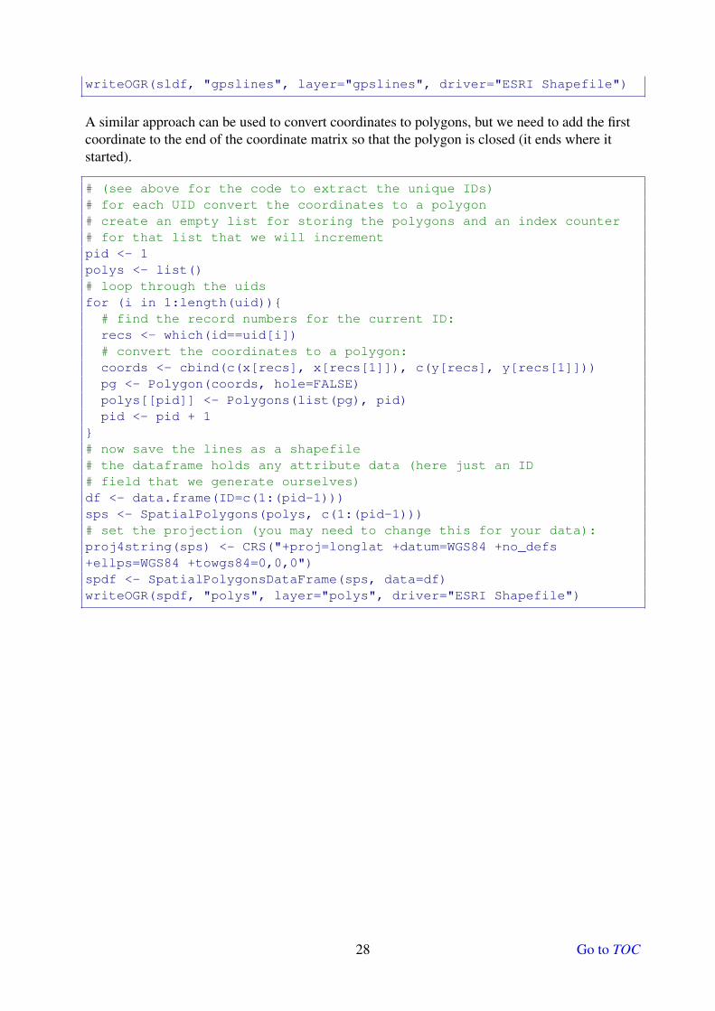
A similar approach can be used to convert coordinates to polygons, but we need to add the firstcoordinate to the end of the coordinate matrix so that the polygon is closed (it ends where itstarted).

# (see above for the code to extract the unique IDs)# for each UID convert the coordinates to a polygon# create an empty list for storing the polygons and an index counter# for that list that we will incrementpid <- 1polys <- list()# loop through the uidsfor (i in 1:length(uid)){

# find the record numbers for the current ID:recs <- which(id==uid[i])# convert the coordinates to a polygon:coords <- cbind(c(x[recs], x[recs[1]]), c(y[recs], y[recs[1]]))pg <- Polygon(coords, hole=FALSE)polys[[pid]] <- Polygons(list(pg), pid)pid <- pid + 1

}# now save the lines as a shapefile# the dataframe holds any attribute data (here just an ID# field that we generate ourselves)df <- data.frame(ID=c(1:(pid-1)))sps <- SpatialPolygons(polys, c(1:(pid-1)))# set the projection (you may need to change this for your data):proj4string(sps) <- CRS("+proj=longlat +datum=WGS84 +no_defs+ellps=WGS84 +towgs84=0,0,0")spdf <- SpatialPolygonsDataFrame(sps, data=df)writeOGR(spdf, "polys", layer="polys", driver="ESRI Shapefile")

28 Go to TOC

15 Exercises

15.1 Landcover of Australia

Create a new R script file using your favourite R text editor and build a workflow to address eachof the following tasks.

1. Load the Australia landcover raster (australialandcov.tif).

2. Load the Australia mainland boundaries polygon dataset (mainland projected.shp)

3. Plot the Australia landcover raster with the polygon boundaries overlaid on top (withtransparent fill). Note that the landcover raster includes more than Australia. For thisexercise we want to restrict our plots and analysis to Australia.

4. Clip the landcover raster to the polygons. Replot the landcover raster and the boundarypolygons to make sure that only areas within the boundary polygons have landcover data.

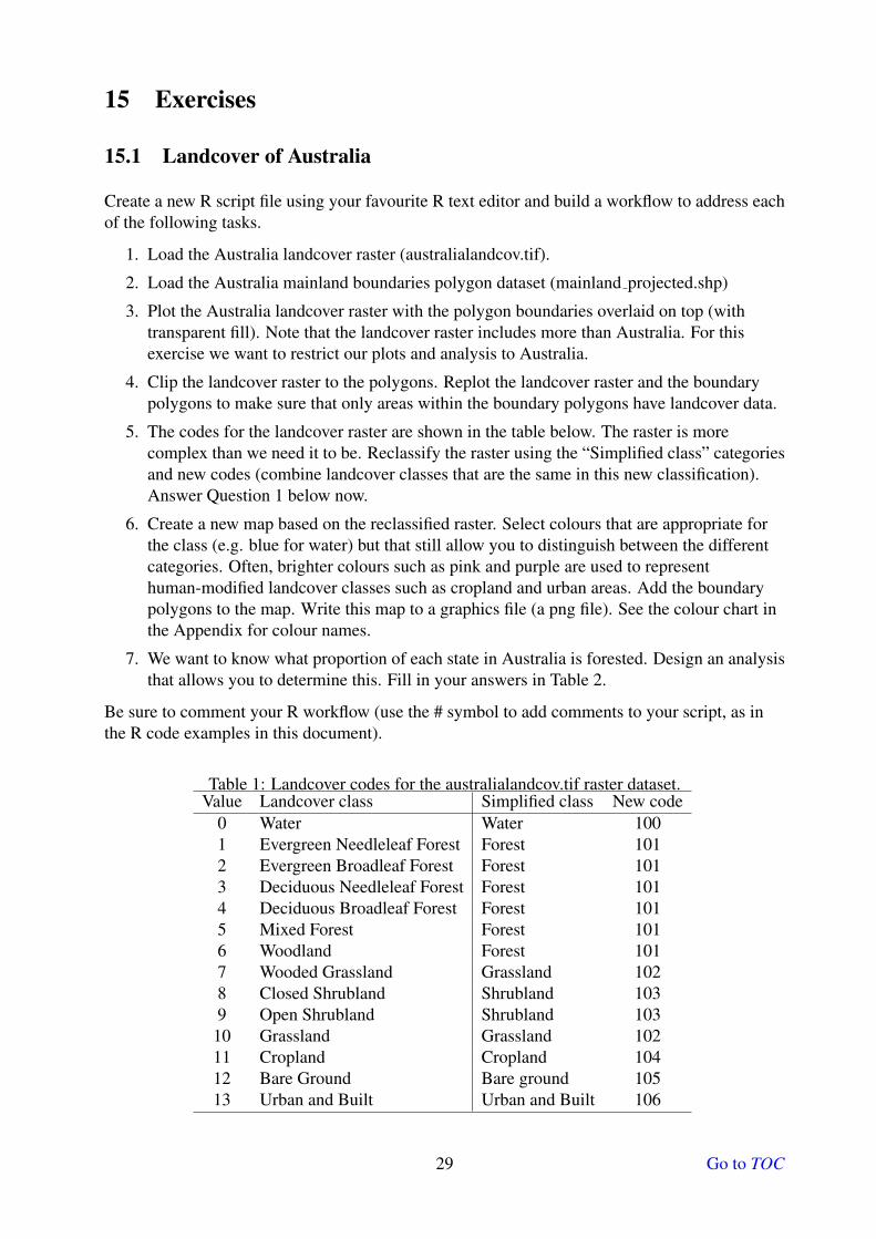
5. The codes for the landcover raster are shown in the table below. The raster is morecomplex than we need it to be. Reclassify the raster using the “Simplified class” categoriesand new codes (combine landcover classes that are the same in this new classification).Answer Question 1 below now.

6. Create a new map based on the reclassified raster. Select colours that are appropriate forthe class (e.g. blue for water) but that still allow you to distinguish between the differentcategories. Often, brighter colours such as pink and purple are used to representhuman-modified landcover classes such as cropland and urban areas. Add the boundarypolygons to the map. Write this map to a graphics file (a png file). See the colour chart inthe Appendix for colour names.

7. We want to know what proportion of each state in Australia is forested. Design an analysisthat allows you to determine this. Fill in your answers in Table 2.

Be sure to comment your R workflow (use the # symbol to add comments to your script, as inthe R code examples in this document).

Table 1: Landcover codes for the australialandcov.tif raster dataset.Value Landcover class Simplified class New code

0 Water Water 1001 Evergreen Needleleaf Forest Forest 1012 Evergreen Broadleaf Forest Forest 1013 Deciduous Needleleaf Forest Forest 1014 Deciduous Broadleaf Forest Forest 1015 Mixed Forest Forest 1016 Woodland Forest 1017 Wooded Grassland Grassland 1028 Closed Shrubland Shrubland 1039 Open Shrubland Shrubland 103

10 Grassland Grassland 10211 Cropland Cropland 10412 Bare Ground Bare ground 10513 Urban and Built Urban and Built 106

29 Go to TOC

15.1.1 Questions

1. There are several ways the reclassification matrix could be specified. Write down twomatrices that could be used to perform the reclassification.

2. Record your estimates of the proportion of each state/territory that is forested in the tablebelow.

Table 2: Austrlian states and territories.State / Territory Abbreviation Proportion forested

Australian Capital Territory ACT

Jervis Bay Territory JBT

New South Wales NSW

Northern Territory NT

Queensland QLD

South Australia SA

Tasmania TAS

Victoria VIC

Western Australia WA

3. Which state has the most forest?

30 Go to TOC

15.2 Generating random points and extracting values

Create a new R script file using your favourite R text editor and build a workflow to address eachof the following tasks.

1. Load the elevation of Australia elevation dataset (SRTM GTOPO u30 australia.tif).

2. Load the state boundaries vector layer (mainlands projected.shp) and extract the polygonfor Queensland (code QLD).

3. Clip the elevation raster based on this Queensland polygon.

4. Create a slope raster based on the clipped elevation raster.

5. Generate 1000 random points based on the clipped elevation layer.

6. Extract elevation and slope values for the random points from the raster datasets.

7. Create a plot in R of the relationship between elevation (x axis) and slope (y axis). See the?plot command.

Be sure to comment your R workflow (use the # symbol to add comments to your script, as inthe R code examples in this document).

15.3 Importing and reprojecting GPS data

The final exercise is more difficult and you will be doing very well if you are able to do completeit. The terminology is sometimes rather obscure and figuring out the various types of spatialobjects in R can be frustrating. But the examples provided earlier provide all the informationrequired to complete the problem.

Your task is to import some animal movement telemetry data, convert the points to lines,reproject the data, and then write the lines as a shapefile. The data is a publicly available dataseton the data archiving website Movebank for migratory Burchell’s zebra (Equus burchellii) innorthern Botswana (Bartlam-Brooks & Harris 2013). Movement data represents a time-series ofGPS locations of an animal, collected by attaching a geolocation device (e.g. a GPS collar) tothe animal. This dataset contains data for 7 zebra.

Create a new R script file using your favourite R text editor and build a workflow to address eachof the following tasks.

1. Read the dataset into R using: data <- read.csv("zebradata.csv")

2. Understand how the data is organised: head(data)

3. Extract the x and y coordinates from this dataset to an x and y variable in R

4. Extract the animal identifier to an id variable in R

5. Create one SpatialLine for each animal (converting the time-series of points to aSpatialLine), storing the SpatialLine objects in a list

6. Convert the SpatialLine list to a SpatialLines object

7. Define the projection (WGS 84, EPSG code 4326)

8. Reproject the data to Africa Albers Equal Area Conic (you need to find the Proj.4 string)

9. Write the data as a line shapefile

31 Go to TOC

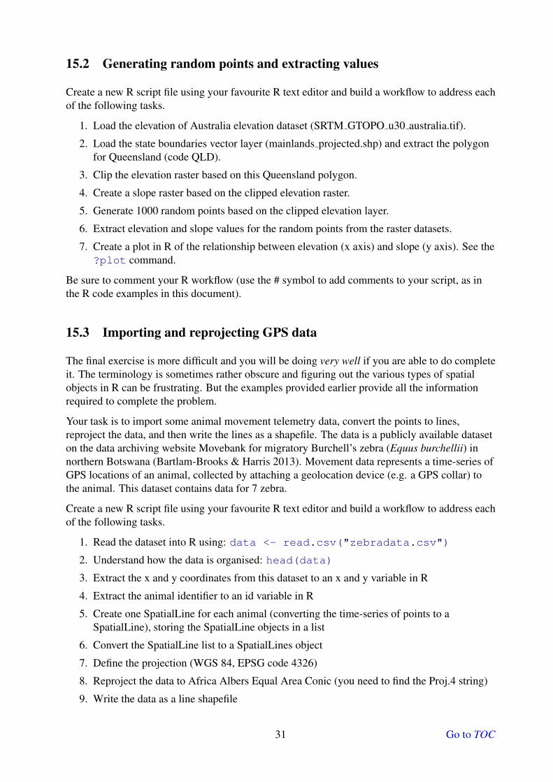
10. Plot the lines with a different colour for each line

Note that a handy way of generating random colours is:

# set the number of colours to generate:ncol <- 7# generate random colours:cols=rgb(runif(ncol), runif(ncol), runif(ncol))# to use the colors in the plot commandplot(mydata, col=cols)

Dataset reference: Bartlam-Brooks HLA and Harris S (2013) Data from: In search of greenerpastures: using satellite images to predict the effects of environmental change on zebramigration. Movebank Data Repository. doi:10.5441/001/1.f3550b4fhttps://www.datarepository.movebank.org/handle/10255/move.343

32 Go to TOC

16 Appendix

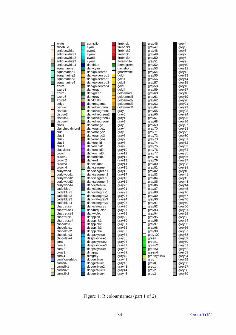
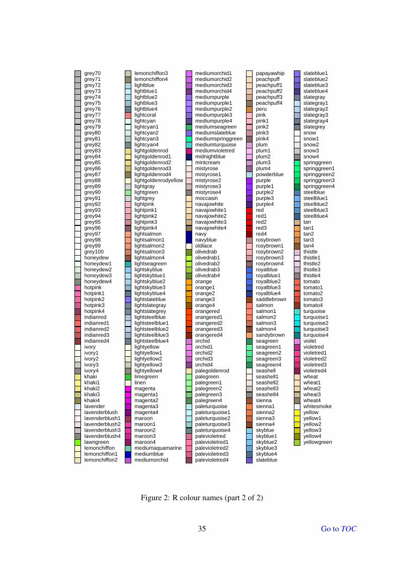
16.1 Specifying colours in R

There are a number of ways of specifying colours in R, but one of the most intuitive is to simplyspecify the name of the colour. There are several hundred pre-defined colours in R that you canchoose from (see the figures below). Note that the names are spelling and case sensitive. Whilethe grey-scale colours support both international and U.S. spelling (grey and gray respectively),some of the colours do not so particular care must be taken to use the spelling provided (e.g.darkslategray1-4, slategray1-4).

33 Go to TOC

whitealiceblueantiquewhiteantiquewhite1antiquewhite2antiquewhite3antiquewhite4aquamarineaquamarine1aquamarine2aquamarine3aquamarine4azureazure1azure2azure3azure4beigebisquebisque1bisque2bisque3bisque4blackblanchedalmondblueblue1blue2blue3blue4bluevioletbrownbrown1brown2brown3brown4burlywoodburlywood1burlywood2burlywood3burlywood4cadetbluecadetblue1cadetblue2cadetblue3cadetblue4chartreusechartreuse1chartreuse2chartreuse3chartreuse4chocolatechocolate1chocolate2chocolate3chocolate4coralcoral1coral2coral3coral4cornflowerbluecornsilkcornsilk1cornsilk2cornsilk3

cornsilk4cyancyan1cyan2cyan3cyan4darkbluedarkcyandarkgoldenroddarkgoldenrod1darkgoldenrod2darkgoldenrod3darkgoldenrod4darkgraydarkgreendarkgreydarkkhakidarkmagentadarkolivegreendarkolivegreen1darkolivegreen2darkolivegreen3darkolivegreen4darkorangedarkorange1darkorange2darkorange3darkorange4darkorchiddarkorchid1darkorchid2darkorchid3darkorchid4darkreddarksalmondarkseagreendarkseagreen1darkseagreen2darkseagreen3darkseagreen4darkslatebluedarkslategraydarkslategray1darkslategray2darkslategray3darkslategray4darkslategreydarkturquoisedarkvioletdeeppinkdeeppink1deeppink2deeppink3deeppink4deepskybluedeepskyblue1deepskyblue2deepskyblue3deepskyblue4dimgraydimgreydodgerbluedodgerblue1dodgerblue2dodgerblue3dodgerblue4

firebrickfirebrick1firebrick2firebrick3firebrick4floralwhiteforestgreengainsboroghostwhitegoldgold1gold2gold3gold4goldenrodgoldenrod1goldenrod2goldenrod3goldenrod4graygray0gray1gray2gray3gray4gray5gray6gray7gray8gray9gray10gray11gray12gray13gray14gray15gray16gray17gray18gray19gray20gray21gray22gray23gray24gray25gray26gray27gray28gray29gray30gray31gray32gray33gray34gray35gray36gray37gray38gray39gray40gray41gray42gray43gray44gray45

gray46gray47gray48gray49gray50gray51gray52gray53gray54gray55gray56gray57gray58gray59gray60gray61gray62gray63gray64gray65gray66gray67gray68gray69gray70gray71gray72gray73gray74gray75gray76gray77gray78gray79gray80gray81gray82gray83gray84gray85gray86gray87gray88gray89gray90gray91gray92gray93gray94gray95gray96gray97gray98gray99gray100greengreen1green2green3green4greenyellowgreygrey0grey1grey2grey3

grey4grey5grey6grey7grey8grey9grey10grey11grey12grey13grey14grey15grey16grey17grey18grey19grey20grey21grey22grey23grey24grey25grey26grey27grey28grey29grey30grey31grey32grey33grey34grey35grey36grey37grey38grey39grey40grey41grey42grey43grey44grey45grey46grey47grey48grey49grey50grey51grey52grey53grey54grey55grey56grey57grey58grey59grey60grey61grey62grey63grey64grey65grey66grey67grey68grey69

Figure 1: R colour names (part 1 of 2)

34 Go to TOC

grey70grey71grey72grey73grey74grey75grey76grey77grey78grey79grey80grey81grey82grey83grey84grey85grey86grey87grey88grey89grey90grey91grey92grey93grey94grey95grey96grey97grey98grey99grey100honeydewhoneydew1honeydew2honeydew3honeydew4hotpinkhotpink1hotpink2hotpink3hotpink4indianredindianred1indianred2indianred3indianred4ivoryivory1ivory2ivory3ivory4khakikhaki1khaki2khaki3khaki4lavenderlavenderblushlavenderblush1lavenderblush2lavenderblush3lavenderblush4lawngreenlemonchiffonlemonchiffon1lemonchiffon2

lemonchiffon3lemonchiffon4lightbluelightblue1lightblue2lightblue3lightblue4lightcorallightcyanlightcyan1lightcyan2lightcyan3lightcyan4lightgoldenrodlightgoldenrod1lightgoldenrod2lightgoldenrod3lightgoldenrod4lightgoldenrodyellowlightgraylightgreenlightgreylightpinklightpink1lightpink2lightpink3lightpink4lightsalmonlightsalmon1lightsalmon2lightsalmon3lightsalmon4lightseagreenlightskybluelightskyblue1lightskyblue2lightskyblue3lightskyblue4lightslatebluelightslategraylightslategreylightsteelbluelightsteelblue1lightsteelblue2lightsteelblue3lightsteelblue4lightyellowlightyellow1lightyellow2lightyellow3lightyellow4limegreenlinenmagentamagenta1magenta2magenta3magenta4maroonmaroon1maroon2maroon3maroon4mediumaquamarinemediumbluemediumorchid

mediumorchid1mediumorchid2mediumorchid3mediumorchid4mediumpurplemediumpurple1mediumpurple2mediumpurple3mediumpurple4mediumseagreenmediumslatebluemediumspringgreenmediumturquoisemediumvioletredmidnightbluemintcreammistyrosemistyrose1mistyrose2mistyrose3mistyrose4moccasinnavajowhitenavajowhite1navajowhite2navajowhite3navajowhite4navynavyblueoldlaceolivedrabolivedrab1olivedrab2olivedrab3olivedrab4orangeorange1orange2orange3orange4orangeredorangered1orangered2orangered3orangered4orchidorchid1orchid2orchid3orchid4palegoldenrodpalegreenpalegreen1palegreen2palegreen3palegreen4paleturquoisepaleturquoise1paleturquoise2paleturquoise3paleturquoise4palevioletredpalevioletred1palevioletred2palevioletred3palevioletred4

papayawhippeachpuffpeachpuff1peachpuff2peachpuff3peachpuff4perupinkpink1pink2pink3pink4plumplum1plum2plum3plum4powderbluepurplepurple1purple2purple3purple4redred1red2red3red4rosybrownrosybrown1rosybrown2rosybrown3rosybrown4royalblueroyalblue1royalblue2royalblue3royalblue4saddlebrownsalmonsalmon1salmon2salmon3salmon4sandybrownseagreenseagreen1seagreen2seagreen3seagreen4seashellseashell1seashell2seashell3seashell4siennasienna1sienna2sienna3sienna4skyblueskyblue1skyblue2skyblue3skyblue4slateblue

slateblue1slateblue2slateblue3slateblue4slategrayslategray1slategray2slategray3slategray4slategreysnowsnow1snow2snow3snow4springgreenspringgreen1springgreen2springgreen3springgreen4steelbluesteelblue1steelblue2steelblue3steelblue4tantan1tan2tan3tan4thistlethistle1thistle2thistle3thistle4tomatotomato1tomato2tomato3tomato4turquoiseturquoise1turquoise2turquoise3turquoise4violetvioletredvioletred1violetred2violetred3violetred4wheatwheat1wheat2wheat3wheat4whitesmokeyellowyellow1yellow2yellow3yellow4yellowgreen

Figure 2: R colour names (part 2 of 2)

35 Go to TOC