An Introduction to Deep Learning - UCL/ELEN · v = input h1 h2 Figure 1: The deep learning scheme: a greedy unsupervised layer-wise pre-training stage followed by a supervised ﬁne-tuning

An Introduction to Deep LearningLudovic Arnold1,2, Sébastien Rebecchi1, Sylvain Chevallier1, Hélène Paugam-Moisy1,3

1- Tao, INRIA-Saclay, LRI, UMR8623, Université Paris-Sud 11F-91405 Orsay, France2- LIMSI, UMR3251

F-91403 Orsay, France3- Université Lyon 2, LIRIS, UMR5205

F-69676 Bron, France

Abstract. The deep learning paradigm tackles problems on which shal-low architectures (e.g. SVM) are affected by the curse of dimensionality.As part of a two-stage learning scheme involving multiple layers of non-linear processing a set of statistically robust features is automatically ex-tracted from the data. The present tutorial introducing the ESANN deeplearning special session details the state-of-the-art models and summarizesthe current understanding of this learning approach which is a referencefor many difficult classification tasks.

1 Introduction

In statistical machine learning, a major issue is the selection of an appropriatefeature space where input instances have desired properties for solving a par-ticular problem. For example, in the context of supervised learning for binaryclassification, it is often required that the two classes are separable by an hy-perplane. In the case where this property is not directly satisfied in the inputspace, one is given the possibility to map instances into an intermediate featurespace where the classes are linearly separable. This intermediate space can ei-ther be specified explicitly by hand-coded features, be defined implicitly with aso-called kernel function, or be automatically learned. In both of the first cases,it is the user’s responsibility to design the feature space. This can incur a hugecost in terms of computational time or expert knowledge, especially with highlydimensional input spaces, such as when dealing with images.

As for the third alternative, automatically learning the features with deeparchitectures, i.e. architectures composed of multiple layers of nonlinear pro-cessing, can be considered as a relevant choice. Indeed, some highly nonlinearfunctions can be represented much more compactly in terms of number of param-eters with deep architectures than with shallow ones (e.g. SVM). For example,it has been proven that the parity function for n-bit inputs can be coded bya feed-forward neural network with O(log n) hidden layers and O(n) neurons,while a feed-forward neural network with only one hidden layer needs an expo-nential number of the same neurons to perform the same task [1]. Moreover, inthe case of highly varying functions, learning algorithms entirely based on localgeneralization are severely impacted by the curse of dimensionality [2]. Deeparchitectures address this issue with the use of distributed representations andas such may constitute a tractable alternative.

477

ESANN 2011 proceedings, European Symposium on Artificial Neural Networks, Computational Intelligence and Machine Learning. Bruges (Belgium), 27-29 April 2011, i6doc.com publ., ISBN 978-2-87419-044-5. Available from http://www.i6doc.com/en/livre/?GCOI=28001100817300.

v = input

h1

h2

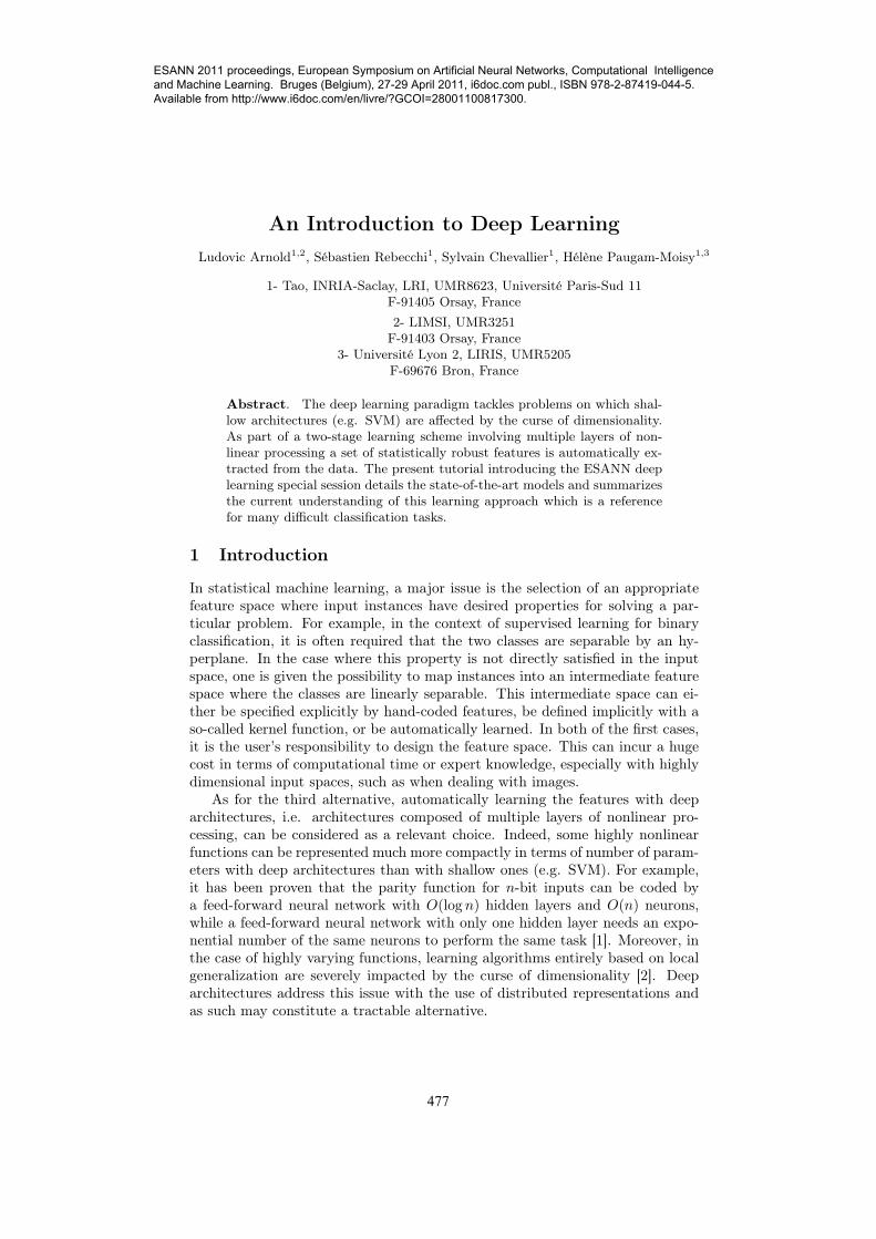
Figure 1: The deep learning scheme: a greedy unsupervised layer-wise pre-training stage followed by a supervised fine-tuning stage affecting all layers.

Unfortunately, training deep architectures is a difficult task and classicalmethods that have proved effective when applied to shallow architectures arenot as efficient when adapted to deep architectures. Adding layers does notnecessarily lead to better solutions. For example, the more the number of layersin a neural network, the lesser the impact of the back-propagation on the firstlayers. The gradient descent then tends to get stuck in local minima or plateaus[3], which is why practitioners have often preferred to limit neural networks toone or two hidden layers.

This issue has been solved by introducing an unsupervised layer-wise pre-training of deep architectures [3, 4]. More precisely, in a deep learning schemeeach layer is treated separately and successively trained in a greedy manner: oncethe previous layers have been trained, a new layer is trained from the encodingof the input data by the previous layers. Then, a supervised fine-tuning stage ofthe whole network can be performed (see Fig. 1).

This paper aims at providing to the reader a better understanding of thedeep learning through a review of the literature and an emphasis of its keyproperties. Section 2 details a widely used deep network model: the deep beliefnetwork or stacked restricted Boltzmann machines. Other models found in deeparchitectures are presented in Sect. 3, i.e. stacked auto-associators, deep kernelmachines and deep convolutional networks. Section 4 summarizes the mainresults in the different application domains, points out the contributions of thedeep learning scheme and concludes the tutorial.

2 Deep learning with RBMs

2.1 Restricted Boltzmann Machines

Restricted Boltzmann Machines (RBMs) are at the intersection of several fieldsof study and benefit from a rich theoretical framework [5, 6]. First, we will

478


Figure 2: The RBM architecture with a visible (v) and a hidden (h) layers.

present them as a probabilistic model before showing how the neural networkequations arise naturally.

An RBM defines a probability distribution p on data vectors v as follows:

p(v) =∑h

e−E(v,h)∑u,g e

−E(u,g). (1)

The variable v is the input vector and the variable h corresponds to unob-served features [7] that can be thought of as hidden causes not available in theoriginal dataset. An RBM defines a joint probability on both the observed andunobserved variables which are referred to as visible and hidden units respec-tively (see Fig. 2). The distribution is then marginalized over the hidden unitsto give a distribution over the visible units only. The probability distributionis defined by an energy function E (RBMs are a special case of energy-basedmodels [8]), which is usually defined over couples (v,h) of binary vectors by:

E(v,h) = −∑i

aivi −∑j

bjhj −∑i,j

wijvihj , (2)

with ai and bj the biases associated to the input variables vi and hidden variableshj respectively and wij the weights of a pairwise interaction between them. Inaccordance with (1), configurations (v,h) with a low energy are given a highprobability whereas a high energy corresponds to a low probability.

The energy function above is crafted to make the conditional probabilitiesp(h|v) and p(v|h) tractable. The computation is done using the usual neuralnetwork propagation rule (see Fig. 2) with:

p(v|h) =∏i

p(vi|h) and p(vi = 1|h) = sigm

⎛⎝aj +

∑j

hjwij

⎞⎠ ,

p(h|v) =∏j

p(hj |v) and p(hj = 1|v) = sigm

(bj +

∑i

viwij

), (3)

where sigm(x) = 1/(1 + exp(−x)) is the logistic activation function.The model with the energy function (2) defines a distribution over binary

vectors and, as such, is not suitable for continuous valued data. To address this

479


issue, E can be appropriately modified to define the Gaussian-Bernoulli RBMby including a quadratic term on the visible units [3]:

E(v,h) =∑i

(vi − ai)2

2σ2i

−∑j

bjhj −∑i,j

wijviσi

hj ,

where σi represents the variance of the input variable vi. Using this energyfunction, the conditional probability p(h|v) is almost unchanged but p(v|h)becomes a multivariate Gaussian with mean ai + σi

∑j wijhj and a diagonal

covariance matrix:

p(vi = x|h) = 1

σi

√2π

· e−

(x− ai − σi

∑j wijhj

)22σ2

i ,

p(hj = 1|v) = sigm

(bj +

∑i

viσi

wij

). (4)

In a deep architecture using Gaussian-Bernoulli RBM, only the first layeris real-valued whereas all the others have binary units. Other variations of theenergy function are given in [3, 9, 10] to address the issue of continuous valuedinputs.

2.2 Learning with RBMs and Contrastive Divergence

In order to train RBMs as a probabilistic model, the natural criterion to maxi-mize is the log-likelihood. This can be done with gradient ascent from a trainingset D likewise:

∂ log p(D)

∂wij=

∑x∈D

∂ log p(x)

∂wij

=∑x∈D

∑g

∂E(x,g)

∂wije−E(x,g)

∑g e

−E(x,g)−∑x∈D

∑u

∑g

∂E(u,g)

∂wije−E(u,g)

∑u

∑g e

−E(u,g),

= Edata

[∂E(x,g)

∂wij

]− Emodel

[∂E(u,g)

∂wij

],

where the first term is the expectation of ∂E(x,g)∂wij

when the input variables are setto an input vector x and the hidden variables are sampled according to the condi-tional distribution p(h|x). The second term is an expectation of ∂E(u,g)

∂wijwhen u

and g are sampled according to the joint distribution of the RBM p(u,g) and isintractable. It can however be approximated with a Markov chain Monte Carloalgorithm such as Gibbs sampling: starting from any configuration (v0,h0), one

480


samples ht according to p(h|vt−1) and vt according to p(v|ht) until the sample(vt,ht) is distributed closely enough to the target distribution p(v,h).

In practice, the number of steps can be greatly reduced by starting theMarkov chain with a sample from the training dataset and assuming that themodel is not too far from the target distribution. This is the idea behind theContrastive Divergence (CD) learning algorithm [11]. Although the maximizedcriterion is not the log-likelihood anymore, experimental results show that gra-dient updates almost always improve the likelihood of the model [11]. Moreover,the improvement to the likelihood tend to zero as the length of the chain in-creases [12], an argument which supports running the chain for a few steps only.Notice that the possibility to use only the sign of the CD update is explored inthe present special session [13].

2.3 From stacked RBMs to deep belief networks

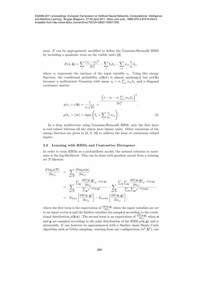
In an RBM, the hidden variables are independent conditionally to the visiblevariables, but they are not statistically independent. Stacking RBMs aims atlearning these dependencies with another RBM. The visible layer of each RBM ofthe stack is set to the hidden layer of the previous RBM (see Fig. 3). Followingthe deep learning scheme, the first RBM is trained from the input instancesand other RBMs are trained sequentially after that. Stacking RBMs increases abound on the log-likelihood [14], which supports the expectation to improve theperformance of the model by adding layers.

Figure 3: The stacked RBMs architecture.

A stacked RBMs architecture is a deep generative model. Patterns generatedfrom the top RBM can be propagated back to the input layer using only theconditional probabilities as in a belief network. This setup is referred to as aDeep Belief Network [4].

481


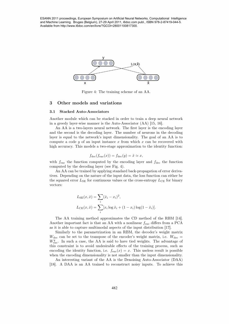
Figure 4: The training scheme of an AA.

3 Other models and variations

3.1 Stacked Auto-Associators

Another module which can be stacked in order to train a deep neural networkin a greedy layer-wise manner is the Auto-Associator (AA) [15, 16].

An AA is a two-layers neural network. The first layer is the encoding layerand the second is the decoding layer. The number of neurons in the decodinglayer is equal to the network’s input dimensionality. The goal of an AA is tocompute a code y of an input instance x from which x can be recovered withhigh accuracy. This models a two-stage approximation to the identity function:

fdec(fenc(x)) = fdec(y) = x̂ � x,

with fenc the function computed by the encoding layer and fdec the functioncomputed by the decoding layer (see Fig. 4).

An AA can be trained by applying standard back-propagation of error deriva-tives. Depending on the nature of the input data, the loss function can either bethe squared error LSE for continuous values or the cross-entropy LCE for binaryvectors:

LSE(x, x̂) =∑i

(x̂i − xi)2,

LCE(x, x̂) =∑i

[xi log x̂i + (1− xi) log(1− x̂i)].

The AA training method approximates the CD method of the RBM [14].Another important fact is that an AA with a nonlinear fenc differs from a PCAas it is able to capture multimodal aspects of the input distribution [17].

Similarly to the parametrization in an RBM, the decoder’s weight matrixWdec can be set to the transpose of the encoder’s weight matrix, i.e. Wdec =W ᵀ

enc. In such a case, the AA is said to have tied weights. The advantage ofthis constraint is to avoid undesirable effects of the training process, such asencoding the identity function, i.e. fenc(x) = x. This useless result is possiblewhen the encoding dimensionality is not smaller than the input dimensionality.

An interesting variant of the AA is the Denoising Auto-Associator (DAA)[18]. A DAA is an AA trained to reconstruct noisy inputs. To achieve this

482


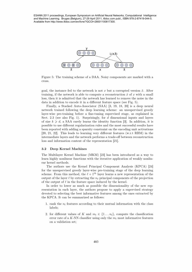
Figure 5: The training scheme of a DAA. Noisy components are marked with across.

goal, the instance fed to the network is not x but a corrupted version x̃. Aftertraining, if the network is able to compute a reconstruction x̂ of x with a smallloss, then it is admitted that the network has learned to remove the noise in thedata in addition to encode it in a different feature space (see Fig. 5).

Finally, a Stacked Auto-Associator (SAA) [3, 19, 18, 20] is a deep neuralnetwork trained following the deep learning scheme: an unsupervised greedylayer-wise pre-training before a fine-tuning supervised stage, as explained inSect. 2.3 (see also Fig. 1). Surprisingly, for d dimensional inputs and layersof size k � d, a SAA rarely learns the identity function [3]. In addition, it ispossible to use different regularization rules and the most successful results havebeen reported with adding a sparsity constraint on the encoding unit activations[20, 21, 22]. This leads to learning very different features (w.r.t RBM) in theintermediate layers and the network performs a trade-off between reconstructionloss and information content of the representation [21].

3.2 Deep Kernel Machines

The Multilayer Kernel Machine (MKM) [23] has been introduced as a way tolearn highly nonlinear functions with the iterative application of weakly nonlin-ear kernel methods.

The authors use the Kernel Principal Component Analysis (KPCA) [24]for the unsupervised greedy layer-wise pre-training stage of the deep learningscheme. From this method, the �+ 1th layer learns a new representation of theoutput of the layer � by extracting the n� principal components of the projectionof the output of � in the feature space induced by the kernel.

In order to lower as much as possible the dimensionality of the new rep-resentation in each layer, the authors propose to apply a supervised strategydevoted to selecting the best informative features among the ones extracted bythe KPCA. It can be summarized as follows:

1. rank the nl features according to their mutual information with the classlabels;

2. for different values of K and ml ∈ {1 . . . nl}, compute the classificationerror rate of a K-NN classifier using only the ml most informative featureson a validation set;

483


3. the value of ml with which the classifier has reached the lowest error ratedetermines the number of features to retain.

However, the main drawback of using KPCA as the building block of an MKMlies in the fact that the feature selection process must be done separately andthus requires a time-expensive cross validation stage. To get rid of this issuewhen training an MKM it is proposed in this special session [25] to use a moreefficient kernel method, the Kernel Partial Least Squares (KPLS).

KPLS does not need cross validation to select the best informative featuresbut embeds this process in the projection strategy [26]. The features are ob-tained iteratively, in a supervised manner. At each iteration j, KPLS selects thejth feature the most correlated with the class labels by solving an updated eigen-problem. The eigenvalue λj of the extracted feature indicates the discriminativeimportance of this feature. The number of features to extract, i.e. the numberof iterations to be performed by KPLS, is determined by a simple thresholdingof λj .

3.3 Deep Convolutional Networks

Convolutional networks are the first examples of deep architectures [27, 28] thathave successfully achieved a good generalization on visual inputs. They are thebest known method for digit recognition [29]. They can be seen as biologicallyinspired architectures, imitating the processing of “simple” and “complex” corti-cal cells which respectively extract orientations information (similar to a Gaborfiltering) and compositions of these orientations.

The main idea of convolutional networks is to combine local computations(convolution of the signal with weight sharing units) and pooling. The convo-lutions are intended to give translation invariance to the system, as the weightsdepend only on spatial separation and not on spatial position. The pooling al-lows to construct a more abstract set of features through nonlinear combinationof the previous level features, taking into account the local topology of the inputdata. By alternating convolution layers and pooling layers, the network succes-sively extracts and combines local features to construct a good representation ofthe input. The connectivity of the convolutional networks, where each unit in aconvolution or a pooling layer is only connected to a small subset of the precedinglayer, allows to train networks with as much as 7 hidden layers. The supervisedlearning is easily achieved, through an error gradient backpropagation.

On the one hand, convolutional framework has been applied to RBM andDBN [10, 30, 31]. In [31] the authors derive a generative pooling strategy whichscales well with image size and they show that the intermediate representationsare more abstract in the higher layer (from edges in the lower layers to objectparts in the higher). On the other hand, the unsupervised pre-training stage ofdeep learning have been applied to convolutional networks [32] and can greatlyreduce the number of labeled examples required. Furthermore, deep convolu-tional networks with sparse regularization [33] yield very promising results fordifficult visual detection tasks, such as pedestrian detection.

484


4 Discussion

4.1 What are the applicative domains for deep learning?

Deep learning architectures express their full potential when dealing with highlyvarying functions, requiring a high number of labeled samples to be captured byshallow architectures. Unsupervised pre-training allows, in practice, to achievegood generalization performance when the training set is of limited size by po-sitioning the network in a region of the parameter space where the supervisedgradient descent is less likely to fall in a local minimum of the loss function.Deep networks have been largely applied to visual classification databases suchas handwritten digits1, object categories2 3 4, pedestrian detection [33] or off-road robot navigation [34], and also on acoustic signals to perform audio clas-sification [35]. In natural language processing, a very interesting approach [36]gives a proof that deep architectures can perform multi-task learning, givingstate-of-the-art results on difficult tasks like semantic role labeling. Deep archi-tectures can also be applied to regression with Gaussian processes [37] and timeseries prediction [38]. In the latter, the conditional RBM have given promisingresults.

Another interesting application area is highly nonlinear data compression.To reduce the dimensionality of an input instance, it is sufficient for a deeparchitecture that the number of units in its last layer is smaller than its inputdimensionality. In practice, limiting the size of a neuron layer can promote in-teresting nonlinear structure of the data. Moreover, adding layers to a neuralnetwork can lead to learning more abstract features, from which input instancescan be coded with high accuracy in a more compact form. Reducing the di-mensionality of data has been presented as one of the first application of deeplearning [39]. This approach is very efficient to perform semantic hashing ontext documents [22, 40], where the codes generated by the deepest layer areused to build a hash table from a set of documents. Retrived documents arethose whose code differs only by a few bits from the query document code. Asimilar approach for a large scale image database is presented in this specialsession [41].

4.2 Open questions and future directions

A significant part of the ongoing research aims at improving the deep networksbuilding blocks For RBMs, several propositions have been made to use real-valued units rather than binary ones either by integrating the covariance of thevisible units in the hidden units update [42] or by approximating real-valuedunits by noisy rectified linear units [9, 10]. For AAs, the denoising criterion isparticularly investigated since it achieves very good results on visual classifica-tion tasks [43].

1MNIST: http://yann.lecun.com/exdb/mnist/2Caltech-101: http://www.vision.caltech.edu/Image_Datasets/Caltech101/3NORB: http://www.cs.nyu.edu/~ylclab/data/norb-v1.0/4CIFAR-10: http://www.cs.utoronto.ca/~kriz/cifar.html

485


Because the construction of good intermediate representations is a crucialpart of deep learning, a meaningful approach is to study the response of theindividual units in each layer. An effective strategy is to find the input patternthat maximizes the activation of a given unit, starting from a random input andperforming a gradient ascent [44].

A major interrogation underlying the deep learning scheme concerns the roleof the unsupervised pre-training. In [44], the authors argue that pre-training actsas an unusual form of regularization. By selecting a region in the parameter spacewhich is not always better than a random one, pre-training systematically leadsto better generalization. The authors provide results showing that pre-trainingdoes not act as an optimization procedure which selects the region of the pa-rameter space where the basins of attraction are the deepest. Pre-training onlymodifies the starting point of supervised training and the regularization effectdoes not vanish when the number of data increases. Deep learning breaks downthe problem of optimizing lower layers given that the upper layers have not yetbeen trained. Lower layers extract robust and disentangled representations ofthe factors of variations (e.g. on images: translation, rotation, scaling), whereashigher layers select and combine these representations. A fusion of the unsuper-vised and supervised paradigms in one single training scheme is an interestingway to explore.

Choosing the correct dimensions of a deep architecture is not an obviousprocess and the results shown in [29] open new perspectives on this topic. Aconvolution network with a random filter bank and with the correct nonlinearitiescan achieve near state-of-the-art results when there is few training labeled data(such as in the Caltech-101 dataset). It has been shown that the architecture ofconvolutional network has a major influence on the performance and that it ispossible to achieve a very fast architecture selection using only random weightsand no time-consuming learning procedure [45]. This, along with the work of[46], points toward new directions for answering the difficult question of how toefficiently set the sizes of layers in deep networks.

4.3 Conclusion

The strength of deep architectures is to stack multiple layers of nonlinear pro-cessing, a process which is well suited to capture highly varying functions with acompact set of parameters. The deep learning scheme, based on a greedy layer-wise unsupervised pre-training, allows to position deep networks in a parameterspace region where the supervised fine-tuning avoids local minima. Deep learn-ing methods achieve very good accuracy, often the best one, for tasks where alarge set of data is available, even if only a small number of instances are la-beled. This approach raises many theoretical and practical questions, which areinvestigated by a growing and very active research community and casts a newlight on our understanding of neural networks and deep architectures.

486


Acknowledgements

This work was supported by the French ANR as part of the ASAP project undergrant ANR_09_EMER_001_04.

References[1] Y. Bengio and Y. LeCun. Scaling learning algorithms towards AI. In Large-Scale Kernel

Machines. 2007.

[2] Y. Bengio, O. Delalleau, and N. Le Roux. The curse of highly variable functions for localkernel machines. In NIPS, 2005.

[3] Y. Bengio, P. Lamblin, V. Popovici, and H. Larochelle. Greedy layer-wise training of deepnetworks. In NIPS, 2007.

[4] G. E. Hinton, S. Osindero, and Yee-Whye Teh. A fast learning algorithm for deep beliefnets. Neur. Comput., 18:1527–1554, 2006.

[5] P. Smolensky. Information processing in dynamical systems: Foundations of harmonytheory. In Parallel Distributed Processing, pages 194–281. 1986.

[6] D. H . Ackley, G. E . Hinton, and T. J . Sejnowski. A learning algorithm for Boltzmannmachines. Cognitive Science, 9:147–169, 1985.

[7] Z. Ghahramani. Unsupervised learning. In Adv. Lect. Mach. Learn., pages 72–112. 2004.

[8] M. Ranzato, Y.-L. Boureau, S. Chopra, and Y. LeCun. A unified energy-based frameworkfor unsupervised learning. In AISTATS, 2007.

[9] V. Nair and G. E. Hinton. Rectified linear units improve restricted Boltzmann machines.In ICML, 2010.

[10] A. Krizhevsky. Convolutional deep belief networks on CIFAR-10. Technical report, Univ.Toronto, 2010.

[11] G. E. Hinton. Training products of experts by minimizing contrastive divergence. Neur.Comput., 14:1771–1800, 2002.

[12] Y. Bengio and O. Delalleau. Justifying and generalizing contrastive divergence. Neur.Comput., 21:1601–1621, 2009.

[13] A. Fischer and C. Igel. Training RBMs depending on the signs of the CD approximationof the log-likelihood derivatives. In ESANN, 2011.

[14] Y. Bengio. Learning deep architectures for AI. Foundations and Trends in MachineLearning, 2:1–127, 2009.

[15] H. Bourlard and Y. Kamp. Auto-association by multilayer perceptrons and singular valuedecomposition. Biological Cybernetics, 59:291–294, 1988.

[16] G. E. Hinton. Connectionist learning procedures. Artificial Intelligence, 40:185–234, 1989.

[17] N. Japkowicz, S. J. Hanson, and M. A. Gluck. Nonlinear autoassociation is not equivalentto PCA. Neur. Comput., 12:531–545, 2000.

[18] P. Vincent, H. Larochelle, Y. Bengio, and P.-A. Manzagol. Extracting and composingrobust features with denoising autoencoders. In ICML, 2008.

[19] H. Larochelle, D. Erhan, A. Courville, J. Bergstra, and Y. Bengio. An empirical evaluationof deep architectures on problems with many factors of variation. In ICML, 2007.

[20] M. A. Ranzato, C. Poultney, S. Chopra, and Y. LeCun. Efficient learning of sparserepresentations with an energy-based model. In NIPS, 2006.

[21] M. Ranzato, Y-L. Boureau, and Y. LeCun. Sparse feature learning for deep belief net-works. In NIPS, 2008.

487


[22] P. Mirowski, M. Ranzato, and Y. LeCun. Dynamic auto-encoders for semantic indexing.In NIPS WS8, 2010.

[23] Y. Cho and L. Saul. Kernel methods for deep learning. In NIPS, 2009.[24] B. Schölkopf, A. J. Smola, and K.-R. Müller. Nonlinear component analysis as a kernel

eigenvalue problem. Neur. Comput., 10:1299–1319, 1998.[25] F. Yger, M. Berar, G. Gasso, and A. Rakotomamonjy. A supervised strategy for deep

kernel machine. In ESANN, 2011.[26] R. Rosipal, L. J. Trejo, and B. Matthews. Kernel PLS-SVC for linear and nonlinear

classification. In ICML, 2003.[27] Y. LeCun, B. Boser, J. S. Denker, D. Henderson, R. E. Howard, W. Hubbard, and L. D.

Jackel. Handwritten digit recognition with a back-propagation network. In NIPS, 1990.[28] Y. LeCun, L. Bottou, Y. Bengio, and P. Haffner. Gradient-based learning applied to

document recognition. Proceedings of the IEEE, 86:2278–2324, 1998.[29] K. Jarrett, K. Kavukcuoglu, M. Ranzato, and Y. LeCun. What is the best multi-stage

architecture for object recognition? In ICCV, 2009.[30] G. Desjardins and Y. Bengio. Empirical evaluation of convolutional RBMs for vision.

Technical report, Univ. Montréal, 2008.[31] H. Lee, R. Grosse, R. Ranganath, and A. Y. Ng. Convolutional deep belief networks for

scalable unsupervised learning of hierarchical representations. In ICML, 2009.[32] K. Kavukcuoglu, M. A. Ranzato, R. Fergus, and Y. LeCun. Learning invariant features

through topographic filter maps. In CVPR, 2009.[33] K. Kavukcuoglu, P. Sermanet, Y.-L. Boureau, K. Gregor, M. Mathieu, and Y. LeCun.

Learning convolutional feature hierarchies for visual recognition. In NIPS. 2010.[34] R. Hadsell, P. Sermanet, J. Ben, A. Erkan, M. Scoffier, K. Kavukcuoglu, U. Muller, and

Y. LeCun. Learning long-range vision for autonomous off-road driving. J. Field Robot.,26:120–144, 2009.

[35] H. Lee, Y. Largman, P. Pham, and A. Y. Ng. Unsupervised feature learning for audioclassification using convolutional deep belief networks. In NIPS, 2009.

[36] R. Collobert and J. Weston. A unified architecture for natural language processing: Deepneural networks with multitask learning. In ICML, 2008.

[37] R. Salakhutdinov and G. E. Hinton. Using deep belief nets to learn covariance kernels forgaussian processes. In NIPS, 2008.

[38] M. D. Zeiler, G. W. Taylor, N. F. Troje, and G. E. Hinton. Modeling pigeon behaviourusing a conditional restricted Boltzmann machine. In ESANN, 2009.

[39] G. E. Hinton and R. Salakhutdinov. Reducing the dimensionality of data with neuralnetworks. Science, 313:504–507, 2006.

[40] R. Salakhutdinov and G. E. Hinton. Semantic hashing. Int. J. Approximate Reasoning,50:969–978, 2009.

[41] A. Krizhevsky and G. E. Hinton. Using very deep autoencoders for content-based imageretrieval. In ESANN, 2011.

[42] M. Ranzato, A. Krizhevsky, and G. E. Hinton. Factored 3-way restricted Boltzmannmachines for modeling natural images. In AISTATS, 2010.

[43] P. Vincent, H. Larochelle, I. Lajoie, Y. Bengio, and P.-A. Manzagol. Stacked denoisingautoencoders: Learning useful representations in a deep network with a local denoisingcriterion. J. Mach. Learn. Res., 2010.

[44] D. Erhan, Y. Bengio, A. Courville, P.-A. Manzagol, P. Vincent, and S. Bengio. Why doesunsupervised pre-training help deep learning? J. Mach. Learn. Res., 11:625–660, 2010.

[45] A. Saxe, P. W. Koh, Z. Chen, M. Bhand, B. Suresh, and A. Ng. On random weights andunsupervised feature learning. In NIPS WS8, 2010.

[46] L. Arnold, H. Paugam-Moisy, and M. Sebag. Unsupervised layer-wise model selection indeep neural networks. In ECAI, 2010.

488


Documents

An Introduction to Deep Learning - UCL/ELEN · v = input h1 h2 Figure 1: The deep learning scheme: a greedy unsupervised layer-wise pre-training stage followed by a supervised ﬁne-tuning