1

An Introduction to Deep Learningfor the Physical Layer

Tim O’Shea, Senior Member, IEEE, and Jakob Hoydis, Member, IEEE

Abstract—We present and discuss several novel applicationsof deep learning (DL) for the physical layer. By interpretinga communications system as an autoencoder, we develop afundamental new way to think about communications systemdesign as an end-to-end reconstruction task that seeks to jointlyoptimize transmitter and receiver components in a single process.We show how this idea can be extended to networks of multipletransmitters and receivers and present the concept of radiotransformer networks (RTNs) as a means to incorporate expertdomain knowledge in the machine learning (ML) model. Lastly,we demonstrate the application of convolutional neural networks(CNNs) on raw IQ samples for modulation classification whichachieves competitive accuracy with respect to traditional schemesrelying on expert features. The paper is concluded with adiscussion of open challenges and areas for future investigation.

I. INTRODUCTION

Communications is a field of rich expert knowledge abouthow to model channels of different types [1], [2], compensatefor various hardware imperfections [3], [4], and design optimalsignaling and detection schemes that ensure a reliable transferof data [5]. As such, it is a complex and mature engineeringfield with many distinct areas of investigation which haveall seen diminishing returns with regards to performanceimprovements, in particular on the physical layer. Becauseof this, there is a high bar of performance over which anymachine learning (ML) or deep learning (DL) based approachmust pass in order to provide tangible new benefits.

In domains such as computer vision and natural languageprocessing, DL shines because it is difficult to characterize realworld images or language with rigid mathematical models. Forexample, while it is an almost impossible task to write a robustalgorithm for detection of handwritten digits or objects inimages, it is almost trivial today to implement DL algorithmsthat learn to accomplish this task beyond human levels ofaccuracy [6], [7]. In communications, on the other hand,we can design transmit signals that enable straightforwardalgorithms for symbol detection for a variety of channel andsystem models (e.g., detection of a constellation symbol inadditive white Gaussian noise (AWGN)). Thus, as long as suchmodels sufficiently capture real effects we do not expect DLto yield significant improvements on the physical layer.

Nevertheless, we believe that the DL applications whichwe explore in this paper are a useful and insightful way offundamentally rethinking the communications system design

T. O’Shea is with the Bradley Department of Electrical and ComputerEngineering, Virginia Tech and DeepSig, Arlington, VA, US (oshea@vt.edu).

J. Hoydis is with Nokia Bell Labs, Route de Villejust, 91620 Nozay, France(jakob.hoydis@nokia-bell-labs.com).

problem, and hold promise for performance improvementsin complex communications scenarios that are difficult todescribe with tractable mathematical models. Our main con-tributions are as follows:

• We demonstrate that it is possible to learn full transmitterand receiver implementations for a given channel modelwhich are optimized for a chosen loss function (e.g.,minimizing block error rate (BLER)). Interestingly, such“learned” systems can be competitive with respect to thecurrent state-of-the-art. The key idea here is to representtransmitter, channel, and receiver as one deep neuralnetwork (NN) that can be trained as an autoencoder. Thebeauty of this approach is that it can even be applied tochannel models and loss functions for which the optimalsolutions are unknown.

• We extend this concept to an adversarial network ofmultiple transmitter-receiver pairs competing for capacity.This leads to the interference channel for which findingthe best signaling scheme is a long-standing researchproblem. We demonstrate that such a setup can also berepresented as an NN with multiple inputs and outputs,and that all transmitter and receiver implementationscan be jointly optimized with respect to a common orindividual performance metric(s).

• We introduce radio transformer networks (RTNs) as away to integrate expert knowledge into the DL model.RTNs allow, for example, to carry out predefined cor-rection algorithms (“transformers”) at the receiver (e.g.,multiplication by a complex-valued number, convolutionwith a vector) which may be fed with parameters learnedby another NN. This NN can be integrated into theend-to-end training process of a task performed on thetransformed signal (e.g., symbol detection).

• We study the use of NNs on complex-valued IQ samplesfor the problem of modulation classification and showthat convolutional neural networks (CNNs), which arethe cornerstone of most DL systems for computer vision,can outperform traditional classification techniques basedon expert features. This result mirrors a relentless trendin DL for various domains, where learned features ulti-mately outperform and displace long-used expert features,such as the scale-invariant feature transform (SIFT) [8]and Bag-of-words [9].

The ideas presented in this paper provide a multitude ofinteresting avenues for future research that will be discussedin detail. We hope that these will stimulate wide interest withinthe research community.

arX

iv:1

702.

0083

2v2

[cs

.IT

] 1

1 Ju

l 201

7

2

The rest of this article is structured as follows: Section I-Adiscusses potential benefits of DL for the physical layer. Sec-tion I-B presents related work. Background of deep learning ispresented in Section II. In Section III, several DL applicationsfor communications are presented. Section IV contains anoverview and discussion of open problems and key areas offuture investigation. Section V concludes the article.

A. Potential of DL for the physical layer

Apart from the intellectual beauty of a fully “learned”communications system, there are some reasons why DL couldprovide gains over existing physical layer algorithms.

First, most signal processing algorithms in communicationshave solid foundations in statistics and information theory andare often provably optimal for tractable mathematically mod-els. These are generally linear, stationary, and have Gaussianstatistics. A practical system, however, has many imperfectionsand non-linearities [4] (e.g., non-linear power amplifiers (PAs),finite resolution quantization) that can only be approximatelycaptured by such models. For this reason, a DL-based commu-nications system (or processing block) that does not require amathematically tractable model and that can be optimized fora specific hardware configuration and channel might be ableto better optimize for such imperfections.

Second, one of the guiding principles of communicationssystems design is to split the signal processing into a chainof multiple independent blocks; each executing a well definedand isolated function (e.g., source/channel coding, modulation,channel estimation, equalization). Although this approach hasled to the efficient, versatile, and controllable systems we havetoday, it is not clear that individually optimized processingblocks achieve the best possible end-to-end performance. Forexample, the separation of source and channel coding formany practical channels and short block lengths (see [10] andreferences therein) as well as separate coding and modulation[11] are known to be sub-optimal. Attempts to jointly optimizeeach of these components, e.g., based on factor graphs [12],provide gains but lead to unwieldy and computationally com-plex systems. A learned end-to-end communications systemon the other hand is unlikely to have such a rigid modularstructure as it is optimized for end-to-end performance.

Third, it has been shown that NNs are universal functionapproximators [13] and recent work has shown a remarkablecapacity for algorithmic learning with recurrent NNs [14] thatare known to be Turing-complete [15]. Since the executionof NNs can be highly parallelized on concurrent architecturesand easily implemented with low-precision data types [16],there is evidence that “learned” algorithms taking this formcould be executed faster and at lower energy cost than theirmanually “programmed” counterparts.

Fourth, massively parallel processing architectures withdistributed memory architectures, such as graphic processingunits (GPUs) but also increasingly specialized chips for NNinference (e.g., [17]), have shown to be very energy efficientand capable of impressive computational throughput whenfully utilized by concurrent algorithms [18]. The performanceof such architectures, however, has been largely limited by the

ability of algorithms and higher level programming languagesto make efficient use of them. The inherently concurrent natureof computation and memory access across wide and deepNNs has demonstrated a surprising ability to readily achievehigh resource utilization on these architectures with minimalapplication specific tuning or optimization required.

B. Historical context and related workApplications of ML in communications have a long history

covering a wide range of applications. These comprise channelmodeling and prediction, localization, equalization, decoding,quantization, compression, demodulation, modulation recog-nition, and spectrum sensing to name a few [19], [20] (andreferences therein). However, to the best of our knowledge anddue to the reasons mentioned above, few of these applicationshave been commonly adopted or led to a wide commercialsuccess. It is also interesting that essentially all of theseapplications focus on individual receiver processing tasksalone, while the consideration of the transmitter or a full end-to-end system is entirely missing in the literature.

The advent of open-source DL libraries (see Section II-B)and readily available specialized hardware along with theastonishing progress of DL in computer vision have stimulatedrenewed interest in the application of DL for communicationsand networking [21]. There are currently essentially twodifferent main approaches of applying DL to the physicallayer. The goal is to either improve/augment parts of existingalgorithms with DL, or to completely replace them.

Among the papers falling into the first category are [22],[23] and [24] that consider improved belief propagationchannel decoding and multiple-input multiple-output (MIMO)detection, respectively. These works are inspired by the ideaof deep unfolding [25] of existing iterative algorithms byessentially interpreting each iteration as a set of NN layers.In a similar manner, [26] aims at improving the solution ofsparse linear inverse problems with DL.

In the second category, papers include [27], dealing withblind detection for MIMO systems with low-resolution quan-tization, and [28], in which detection for molecular commu-nications for which no mathematical channel model exists isstudied. The idea of learning to solve complex optimizationtasks for wireless resource allocation, such as power control,is investigated in [29]. Some of us have also demonstratedinitial results in the area of learned end-to-end communicationssystems [30] as well as considered the problems of modula-tion recognition [31], signal compression [32], and channeldecoding [33], [34] with state-of-the art DL tools.

Notations: We use boldface upper- and lower-case letters todenote matrices and column vectors, respectively. For a vectorx, xi denotes its ith element, ‖x‖ its Euclidean norm, xT itstranspose, and x � y the element-wise product with y. Fora matrix X, Xij or [X]ij denotes the (i, j)-element. R andC denote the sets of real and complex numbers, respectively.N (m,R) and CN (m,R) are the multivariate Gaussian andcomplex Gaussian distributions with mean vector m andcovariance matrix R, respectively. Bern(α) is the Bernoullidistribution with success probability α and ∇ is the gradientoperator.

3

II. DEEP LEARNING BASICS

A feedforward NN (or multilayer perceptron (MLP)) withL layers describes a mapping f(r0;θ) : RN0 7→ RNL of aninput vector r0 ∈ RN0 to an output vector rL ∈ RNL throughL iterative processing steps:

r` = f`(r`−1; θ`), ` = 1, . . . , L (1)

where f`(r`−1; θ`) : RN`−1 7→ RN` is the mapping carriedout by the `th layer. This mapping depends not only on theoutput vector r`−1 from the previous layer but also on a setof parameters θ`. Moreover, the mapping can be stochastic,i.e., f` can be a function of some random variables. We useθ = {θ1, . . . , θL} to denote the set of all parameters of thenetwork. The `th layer is called dense or fully-connected iff`(r`−1; θ`) has the form

f`(r`−1; θ`) = σ (W`r`−1 + b`) (2)

where W` ∈ RN`×N`−1 , b` ∈ RN` , and σ(·) is an activationfunction which we will be defined shortly. The set of param-eters for this layer is θ` = {W`,b`}. Table I lists severalother layer types together with their mapping functions andparameters which are used in this manuscript. All layers withstochastic mappings generate a new random mapping eachtime they are called. For example, the noise layer simply addsa Gaussian noise vector with zero mean and covariance matrixβIN`−1

to the input. Thus, it generates a different output for thesame input each time it is called. The activation function σ(·)in (2) introduces a non-linearity which is important for the so-called expressive power of the NN. Without this non-linearitythere would be not much of an advantage of stacking multiplelayers on top of each other. Generally, the activation functionis applied individually to each element of its input vector, i.e.,[σ(u)]i = σ(ui). Some commonly used activation functionsare listed in Table II.1 NNs are generally trained using labeledtraining data, i.e., a set of input-output vector pairs (r0,i, r

?L,i),

i = 1, . . . , S, where r?L,i is the desired output of the neuralnetwork when r0,i is used as input. The goal of the trainingprocess is to minimize the loss

L(θ) =1

S

S∑i=1

l(r?L,i, rL,i) (3)

with respect to the parameters in θ, wherel(u,v) : RNL × RNL 7→ R is the loss function and rL,i

is the output of the NN when r0,i is used as input. Severalrelevant loss functions are provided in Table III. Differentnorms (e.g., L1, L2) of parameters or activations can beadded to the loss function to favor solutions with small orsparse values (a form of regularization). The most popularalgorithm to find good sets of parameters θ is stochasticgradient descent (SGD) which starts with some random initialvalues of θ = θ0 and then updates θ iteratively as

θt+1 = θt − η∇L(θt) (4)

1The linear activation function is typically used at the output layer in thecontext of regression tasks, i.e., estimation of a real-valued vector.

Table I: List of layer types

Name f`(r`−1; θ`) θ`Dense σ (W`r`−1 + b`) W`,b`

Noise r`−1 + n, n ∼ N (0, βIN`−1) none

Dropout [36] d� r`−1, di ∼ Bern(α) none

Normalization e.g.,√

N`−1r`−1

‖r`−1‖2none

Table II: List of activation functions

Name [σ(u)]i Rangelinear ui (−∞,∞)

ReLU [37] max(0, ui) [0,∞)

tanh tanh(ui) (−1, 1)sigmoid 1

1+e−ui(0, 1)

softmax eui∑j e

uj (0, 1)

Table III: List of loss functions

Name l(u,v)

MSE ‖u− v‖22Categorical cross-entropy −

∑j uj log(vj)

where η > 0 is the learning rate and L(θ) is an approximationof the loss function which is computed for a random mini-batch of training examples St ⊂ {1, 2, . . . , S} of size St ateach iteration, i.e.,

L(θ) =1

St

∑i∈St

l(r?L,i, rL,i). (5)

By choosing St small compared to S, the gradient computationcomplexity is significantly reduced while still reducing weightupdate variance. Note that there are many variants of theSGD algorithm which dynamically adapt the learning rateto improve convergence [35, Ch. 8.5]. The gradient in (4)can be very efficiently computed through the backpropagationalgorithm [35, Ch. 6.5]. Definition and training of NNs ofalmost arbitrary shape can be easily done with one of themany existing DL libraries presented in Section II-B.

A. Convolutional layers

Convolutional neural network (CNN) layers were introducedin [6] to provide an efficient learning method for 2D images.By tying adjacent shifts of the same weights together in away similar to that of a filter sliding across an input vector,convolutional layers are able to force the learning of featureswith an invariance to shifts in the input vector. In doing so,they also greatly reduce the model complexity (as measuredby the number of free parameters in the layer’s weight matrix)required to represent equivalent shift-invariant features usingfully connected layers, reducing SGD optimization complexityand improving generalization on appropriate datasets.

In general, a convolutional layer consists of a set of F filterweights Qf ∈ Ra×b, f = 1, . . . , F (F is called the depth),which generate each a so-called feature map Yf ∈ Rn′×m′

from an input matrix X ∈ Rn×m 2 according to the following

2In image processing, X is commonly a three-dimensional tensor with thethird dimension corresponding to color channels. The filters weights are alsothree-dimensional and work on each input channels simultaneously.

4

convolution:

Y fi,j =

a−1∑k=0

b−1∑`=0

Qfa−k,b−`X1+s(i−1)−k,1+s(j−1)−` (6)

where s ≥ 1 is an integer parameter called stride, n′ =1 + bn+a−2

s c and m′ = 1 + bm+b−2s c, and it is assumed

that X is padded with zeros, i.e., Xi,j = 0 for all i /∈ [1, n]and j /∈ [1,m]. The output dimensions can be reduced byeither increasing the stride s or by adding a pooling layer.The pooling layer partitions Y into p× p regions for each ofwhich it computes a single output value, e.g., maximum oraverage value, or L2-norm.

For example, taking a vectorized grayscale image inputconsisting of 28×28 pixels and connecting it to a dense layerwith the same number of activations, results in a single weightmatrix with 784 × 784 = 614, 656 free parameters. On theother hand, if we use a convolutional feature map containingsix filters each sized 5× 5 pixels, we obtain a much reducednumber of free parameters of 6 ·5 ·5 = 150. For the right kindof dataset, this technique can be extremely effective. We willsee an application of convolutional layers in Section III-D. Formore details on CNNs, we refer to [35, Ch. 9].

B. Machine learning libraries

In recent times, numerous tools and algorithms haveemerged that make it easy to build and train large NNs. Toolsto deploy such training routines from high level language tomassively parallel GPU architectures have been key enablers.Among these are Caffe [38], MXNet [39], TensorFlow [40],Theano [41], and Torch [42] (just to name a few), which allowfor high level algorithm definition in various programminglanguages or configuration files, automatic differentiation oftraining loss functions through arbitrarily large networks, andcompilation of the network’s forwards and backwards passesinto hardware optimized concurrent dense matrix algebra ker-nels. Keras [43] provides an additional layer of NN primitiveswith Theano and TensorFlow as its back-end. It has a highlycustomizable interface to quickly experiment with and deploydeep NNs, and has become our primary tool used to generatethe numerical results for this manuscript [44].

C. Network dimensions and training

The term “deep” has become common in recent NN liter-ature, referring to the number of sequential layers within anetwork (but also more generally to the methods commonlyused to train such networks). Depth relates directly to thenumber of iterative operations performed on input data throughsequential layers’ transfer functions. While deep networksallow for numerous iterative transforms on the data, a min-imum latency network would likely be as shallow as possible.“Width” is used to describe the number of output activationsper layer, or for all layers on average, and relates directly tothe memory required by each layer.

Best practice training methods have varied over the years,from direct solution techniques over gradient descent to ge-netic algorithms, each having been favored or considered at

one time (see [35, Ch. 1.2] for a short history of DL). Layer-by-layer pre-training [45] was also a recently popular methodfor scaling training to larger networks where backpropagationonce struggled. However, most systems today are able to trainnetworks which are both wide and deep directly using back-propagation and SGD methods with adaptive learning rates(e.g., Adam [46]), regularization methods to prevent overfitting(e.g., Dropout [36]), and activations functions which reducegradient issues (e.g., ReLU [37]).

III. EXAMPLES OF MACHINE LEARNING APPLICATIONSFOR THE PHYSICAL LAYER

In this section, we will show how to represent an end-to-end communications system as an autoencoder and train it viaSGD. This idea is then extended to multiple transmitters andreceivers and we study as an example the two-user interferencechannel. We will then introduce the concept of RTNs toimprove performance on fading channels, and demonstrate theapplication of CNNs to raw radio frequency time-series datafor the task of modulation classification.

A. Autoencoders for end-to-end communications systems

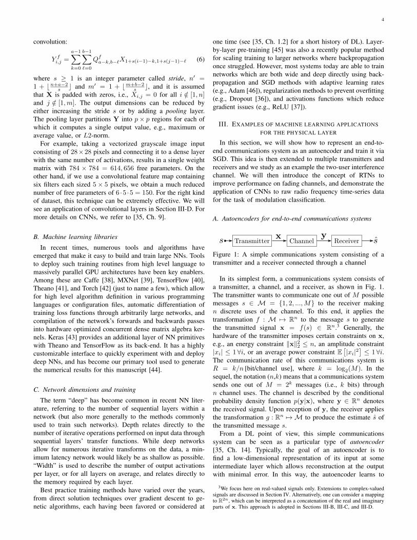
Figure 1: A simple communications system consisting of atransmitter and a receiver connected through a channel

In its simplest form, a communications system consists ofa transmitter, a channel, and a receiver, as shown in Fig. 1.The transmitter wants to communicate one out of M possiblemessages s ∈ M = {1, 2, ...,M} to the receiver makingn discrete uses of the channel. To this end, it applies thetransformation f : M 7→ Rn to the message s to generatethe transmitted signal x = f(s) ∈ Rn.3 Generally, thehardware of the transmitter imposes certain constraints on x,e.g., an energy constraint ‖x‖22 ≤ n, an amplitude constraint|xi| ≤ 1∀i, or an average power constraint E

[|xi|2

]≤ 1∀i.

The communication rate of this communications system isR = k/n [bit/channel use], where k = log2(M). In thesequel, the notation (n,k) means that a communications systemsends one out of M = 2k messages (i.e., k bits) throughn channel uses. The channel is described by the conditionalprobability density function p(y|x), where y ∈ Rn denotesthe received signal. Upon reception of y, the receiver appliesthe transformation g : Rn 7→ M to produce the estimate s ofthe transmitted message s.

From a DL point of view, this simple communicationssystem can be seen as a particular type of autoencoder[35, Ch. 14]. Typically, the goal of an autoencoder is tofind a low-dimensional representation of its input at someintermediate layer which allows reconstruction at the outputwith minimal error. In this way, the autoencoder learns to

3We focus here on real-valued signals only. Extensions to complex-valuedsignals are discussed in Section IV. Alternatively, one can consider a mappingto R2n, which can be interpreted as a concatenation of the real and imaginaryparts of x. This approach is adopted in Sections III-B, III-C, and III-D.

5

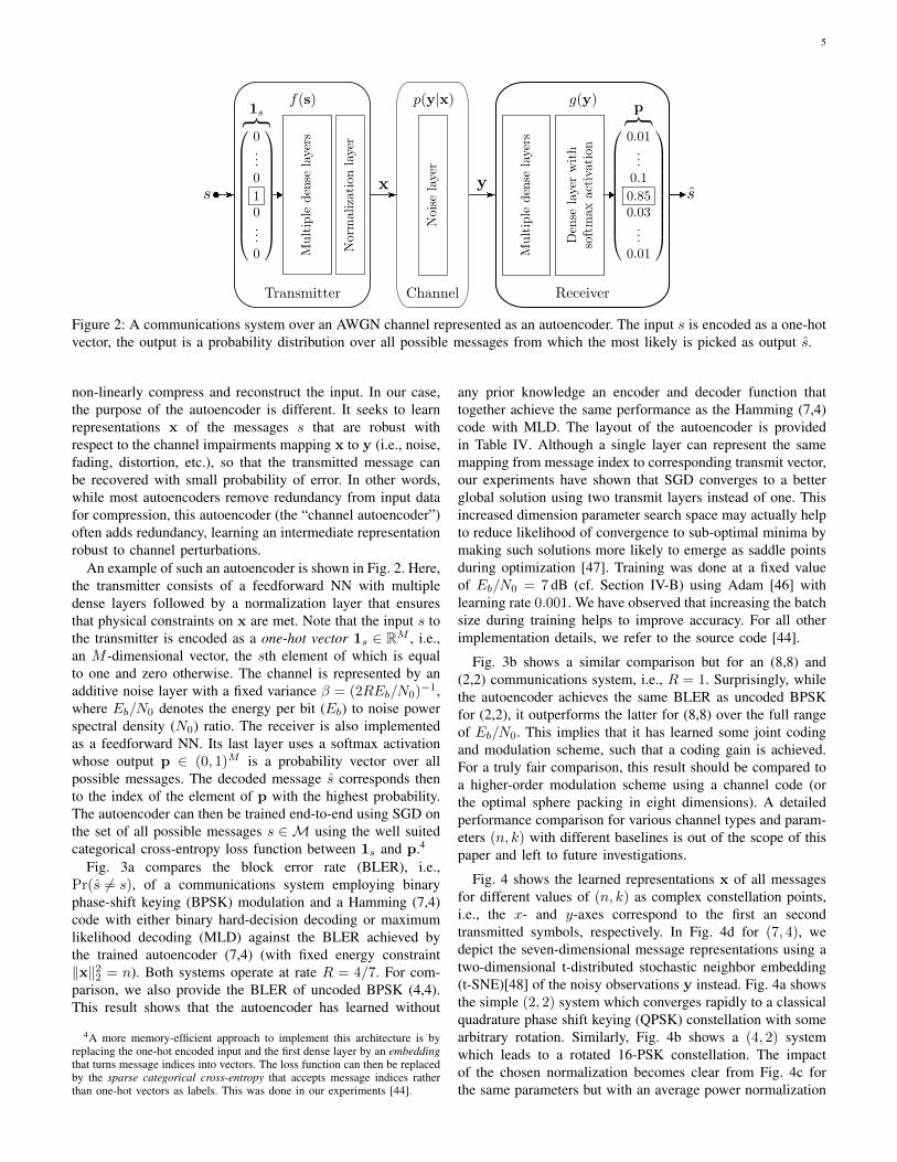
Figure 2: A communications system over an AWGN channel represented as an autoencoder. The input s is encoded as a one-hotvector, the output is a probability distribution over all possible messages from which the most likely is picked as output s.

non-linearly compress and reconstruct the input. In our case,the purpose of the autoencoder is different. It seeks to learnrepresentations x of the messages s that are robust withrespect to the channel impairments mapping x to y (i.e., noise,fading, distortion, etc.), so that the transmitted message canbe recovered with small probability of error. In other words,while most autoencoders remove redundancy from input datafor compression, this autoencoder (the “channel autoencoder”)often adds redundancy, learning an intermediate representationrobust to channel perturbations.

An example of such an autoencoder is shown in Fig. 2. Here,the transmitter consists of a feedforward NN with multipledense layers followed by a normalization layer that ensuresthat physical constraints on x are met. Note that the input s tothe transmitter is encoded as a one-hot vector 1s ∈ RM , i.e.,an M -dimensional vector, the sth element of which is equalto one and zero otherwise. The channel is represented by anadditive noise layer with a fixed variance β = (2REb/N0)−1,where Eb/N0 denotes the energy per bit (Eb) to noise powerspectral density (N0) ratio. The receiver is also implementedas a feedforward NN. Its last layer uses a softmax activationwhose output p ∈ (0, 1)M is a probability vector over allpossible messages. The decoded message s corresponds thento the index of the element of p with the highest probability.The autoencoder can then be trained end-to-end using SGD onthe set of all possible messages s ∈ M using the well suitedcategorical cross-entropy loss function between 1s and p.4

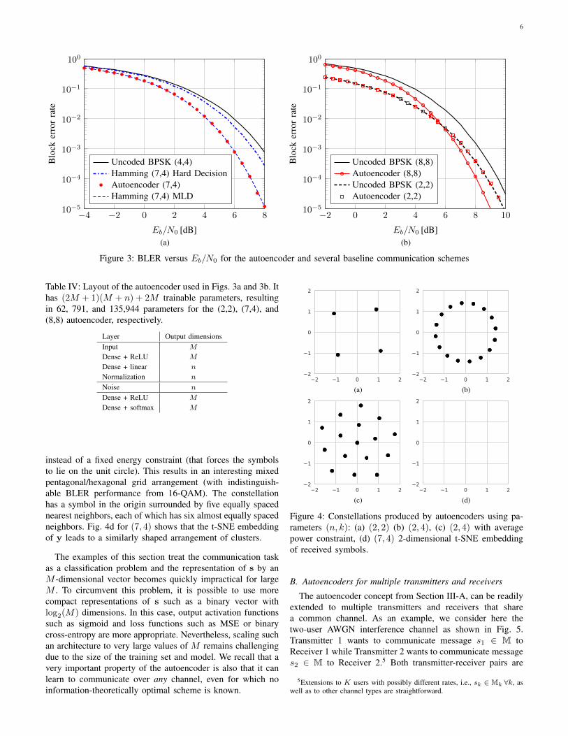
Fig. 3a compares the block error rate (BLER), i.e.,Pr(s 6= s), of a communications system employing binaryphase-shift keying (BPSK) modulation and a Hamming (7,4)code with either binary hard-decision decoding or maximumlikelihood decoding (MLD) against the BLER achieved bythe trained autoencoder (7,4) (with fixed energy constraint‖x‖22 = n). Both systems operate at rate R = 4/7. For com-parison, we also provide the BLER of uncoded BPSK (4,4).This result shows that the autoencoder has learned without

4A more memory-efficient approach to implement this architecture is byreplacing the one-hot encoded input and the first dense layer by an embeddingthat turns message indices into vectors. The loss function can then be replacedby the sparse categorical cross-entropy that accepts message indices ratherthan one-hot vectors as labels. This was done in our experiments [44].

any prior knowledge an encoder and decoder function thattogether achieve the same performance as the Hamming (7,4)code with MLD. The layout of the autoencoder is providedin Table IV. Although a single layer can represent the samemapping from message index to corresponding transmit vector,our experiments have shown that SGD converges to a betterglobal solution using two transmit layers instead of one. Thisincreased dimension parameter search space may actually helpto reduce likelihood of convergence to sub-optimal minima bymaking such solutions more likely to emerge as saddle pointsduring optimization [47]. Training was done at a fixed valueof Eb/N0 = 7 dB (cf. Section IV-B) using Adam [46] withlearning rate 0.001. We have observed that increasing the batchsize during training helps to improve accuracy. For all otherimplementation details, we refer to the source code [44].

Fig. 3b shows a similar comparison but for an (8,8) and(2,2) communications system, i.e., R = 1. Surprisingly, whilethe autoencoder achieves the same BLER as uncoded BPSKfor (2,2), it outperforms the latter for (8,8) over the full rangeof Eb/N0. This implies that it has learned some joint codingand modulation scheme, such that a coding gain is achieved.For a truly fair comparison, this result should be compared toa higher-order modulation scheme using a channel code (orthe optimal sphere packing in eight dimensions). A detailedperformance comparison for various channel types and param-eters (n, k) with different baselines is out of the scope of thispaper and left to future investigations.

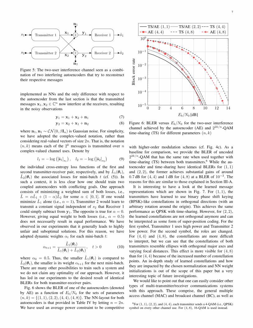
Fig. 4 shows the learned representations x of all messagesfor different values of (n, k) as complex constellation points,i.e., the x- and y-axes correspond to the first an secondtransmitted symbols, respectively. In Fig. 4d for (7, 4), wedepict the seven-dimensional message representations using atwo-dimensional t-distributed stochastic neighbor embedding(t-SNE)[48] of the noisy observations y instead. Fig. 4a showsthe simple (2, 2) system which converges rapidly to a classicalquadrature phase shift keying (QPSK) constellation with somearbitrary rotation. Similarly, Fig. 4b shows a (4, 2) systemwhich leads to a rotated 16-PSK constellation. The impactof the chosen normalization becomes clear from Fig. 4c forthe same parameters but with an average power normalization

6

−4 −2 0 2 4 6 810−5

10−4

10−3

10−2

10−1

100

Eb/N0 [dB]

Blo

cker

ror

rate

Uncoded BPSK (4,4)Hamming (7,4) Hard DecisionAutoencoder (7,4)Hamming (7,4) MLD

(a)

−2 0 2 4 6 8 1010−5

10−4

10−3

10−2

10−1

100

Eb/N0 [dB]

Blo

cker

ror

rate

Uncoded BPSK (8,8)Autoencoder (8,8)Uncoded BPSK (2,2)Autoencoder (2,2)

(b)

Figure 3: BLER versus Eb/N0 for the autoencoder and several baseline communication schemes

Table IV: Layout of the autoencoder used in Figs. 3a and 3b. Ithas (2M + 1)(M + n) + 2M trainable parameters, resultingin 62, 791, and 135,944 parameters for the (2,2), (7,4), and(8,8) autoencoder, respectively.

Layer Output dimensionsInput M

Dense + ReLU M

Dense + linear n

Normalization n

Noise n

Dense + ReLU M

Dense + softmax M

instead of a fixed energy constraint (that forces the symbolsto lie on the unit circle). This results in an interesting mixedpentagonal/hexagonal grid arrangement (with indistinguish-able BLER performance from 16-QAM). The constellationhas a symbol in the origin surrounded by five equally spacednearest neighbors, each of which has six almost equally spacedneighbors. Fig. 4d for (7, 4) shows that the t-SNE embeddingof y leads to a similarly shaped arrangement of clusters.

The examples of this section treat the communication taskas a classification problem and the representation of s by anM -dimensional vector becomes quickly impractical for largeM . To circumvent this problem, it is possible to use morecompact representations of s such as a binary vector withlog2(M) dimensions. In this case, output activation functionssuch as sigmoid and loss functions such as MSE or binarycross-entropy are more appropriate. Nevertheless, scaling suchan architecture to very large values of M remains challengingdue to the size of the training set and model. We recall that avery important property of the autoencoder is also that it canlearn to communicate over any channel, even for which noinformation-theoretically optimal scheme is known.

(a) (b)

(c) (d)

Figure 4: Constellations produced by autoencoders using pa-rameters (n, k): (a) (2, 2) (b) (2, 4), (c) (2, 4) with averagepower constraint, (d) (7, 4) 2-dimensional t-SNE embeddingof received symbols.

B. Autoencoders for multiple transmitters and receivers

The autoencoder concept from Section III-A, can be readilyextended to multiple transmitters and receivers that sharea common channel. As an example, we consider here thetwo-user AWGN interference channel as shown in Fig. 5.Transmitter 1 wants to communicate message s1 ∈ M toReceiver 1 while Transmitter 2 wants to communicate messages2 ∈ M to Receiver 2.5 Both transmitter-receiver pairs are

5Extensions to K users with possibly different rates, i.e., sk ∈ Mk ∀k, aswell as to other channel types are straightforward.

7

Figure 5: The two-user interference channel seen as a combi-nation of two interfering autoencoders that try to reconstructtheir respective messages

implemented as NNs and the only difference with respect tothe autoencoder from the last section is that the transmittedmessages x1,x2 ∈ Cn now interfere at the receivers, resultingin the noisy observations

y1 = x1 + x2 + n1 (7)y2 = x2 + x1 + n2 (8)

where n1,n1 ∼ CN (0, βIn) is Gaussian noise. For simplicity,we have adopted the complex-valued notation, rather thanconsidering real-valued vectors of size 2n. That is, the notation(n, k) means each of the 2k messages is transmitted over ncomplex-valued channel uses. Denote by

l1 = − log([s1]s1

), l2 = − log

([s2]s2

)(9)

the individual cross-entropy loss functions of the first andsecond transmitter-receiver pair, respectively, and by L1(θt),L2(θt) the associated losses for mini-batch t (cf. (5)). Insuch a context, it is less clear how one should train twocoupled autoencoders with conflicting goals. One approachconsists of minimizing a weighted sum of both losses, i.e.,L = αL1 + (1 − α)L2 for some α ∈ [0, 1]. If one wouldminimize L1 alone (i.e., α = 1), Transmitter 2 would learn totransmit a constant signal independent of s2 that Receiver 1could simply subtract from y1. The opposite is true for α = 0.However, giving equal weight to both losses (i.e., α = 0.5)does not necessarily result in equal performance. We haveobserved in our experiments that it generally leads to highlyunfair and suboptimal solutions. For this reason, we haveadopted dynamic weights αt for each mini-batch t:

αt+1 =L1(θt)

L1(θt) + L2(θt), t > 0 (10)

where α0 = 0.5. Thus, the smaller L1(θt) is compared toL2(θt), the smaller is its weight αt+1 for the next mini-batch.There are many other possibilities to train such a system andwe do not claim any optimality of our approach. However, ithas led in our experiments to the desired result of identicalBLERs for both transmitter-receiver pairs.

Fig. 6 shows the BLER of one of the autoencoders (denotedby AE) as a function of Eb/N0 for the sets of parameters(n, k) = {(1, 1), (2, 2), (4, 4), (4, 8)}. The NN-layout for bothautoencoders is that provided in Table IV by letting n = 2n.We have used an average power constraint to be competitive

0 2 4 6 8 10 12 1410−5

10−4

10−3

10−2

10−1

100

Eb/N0 [dB]

Blo

cker

ror

rate

TS/AE (1, 1) TS/AE (2, 2) TS (4, 4)

AE (4, 4) TS (4, 8) AE (4, 8)

Figure 6: BLER versus Eb/N0 for the two-user interferencechannel achieved by the autoencoder (AE) and 22k/n-QAMtime-sharing (TS) for different parameters (n, k)

with higher-order modulation schemes (cf. Fig. 4c). As abaseline for comparison, we provide the BLER of uncoded22k/n-QAM that has the same rate when used together withtime-sharing (TS) between both transmitters.6 While the au-toencoder and time-sharing have identical BLERs for (1, 1)and (2, 2), the former achieves substantial gains of around0.7 dB for (4, 4) and 1 dB for (4, 8) at a BLER of 10−3. Thereasons for this are similar to those explained in Section III-A.

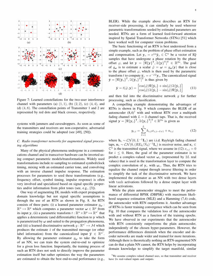
It is interesting to have a look at the learned messagerepresentations which are shown in Fig. 7. For (1, 1), thetransmitters have learned to use binary phase shift keying(BPSK)-like constellations in orthogonal directions (with anarbitrary rotation around the origin). This achieves the sameperformance as QPSK with time-sharing. However, for (2, 2),the learned constellations are not orthogonal anymore and canbe interpreted as some form of super-position coding. For thefirst symbol, Transmitter 1 uses high power and Transmitter 2low power. For the second symbol, the roles are changed.For (4, 4) and (4, 8), the constellations are more difficultto interpret, but we can see that the constellations of bothtransmitters resemble ellipses with orthogonal major axes andvarying focal distances. This effect is more visible for (4, 8)than for (4, 4) because of the increased number of constellationpoints. An in-depth study of learned constellations and howthey are impacted by the chosen normalization and NN weightinitializations is out of the scope of this paper but a veryinteresting topic of future investigations.

We would like to point out that one can easily consider othertypes of multi-transmitter/receiver communications systemswith this approach. These comprise, the general multipleaccess channel (MAC) and broadcast channel (BC), as well as

6For (1, 1), (2, 2), and (4, 4), each transmitter sends a 4-QAM (i.e., QPSK)symbol on every other channel use. For (4, 8), 16-QAM is used instead.

8

(a) (b)

(c)

(d)

Figure 7: Learned constellations for the two-user interferencechannel with parameters (a) (1, 1), (b) (2, 2), (c) (4, 4), and(d) (4, 8). The constellation points of Transmitter 1 and 2 arerepresented by red dots and black crosses, respectively.

systems with jammers and eavesdroppers. As soon as some ofthe transmitters and receivers are non-cooperative, adversarialtraining strategies could be adopted (see [49], [50]).

C. Radio transformer networks for augmented signal process-ing algorithms

Many of the physical phenomena undergone in a communi-cations channel and in transceiver hardware can be inverted us-ing compact parametric models/transformations. Widely usedtransformations include re-sampling to estimated symbol/clocktiming, mixing with an estimated carrier tone, and convolvingwith an inverse channel impulse response. The estimationprocesses for parameters to seed these transformations (e.g.,frequency offset, symbol timing, impulse response) is oftenvery involved and specialized based on signal specific proper-ties and/or information from pilot tones (see, e.g., [3]).

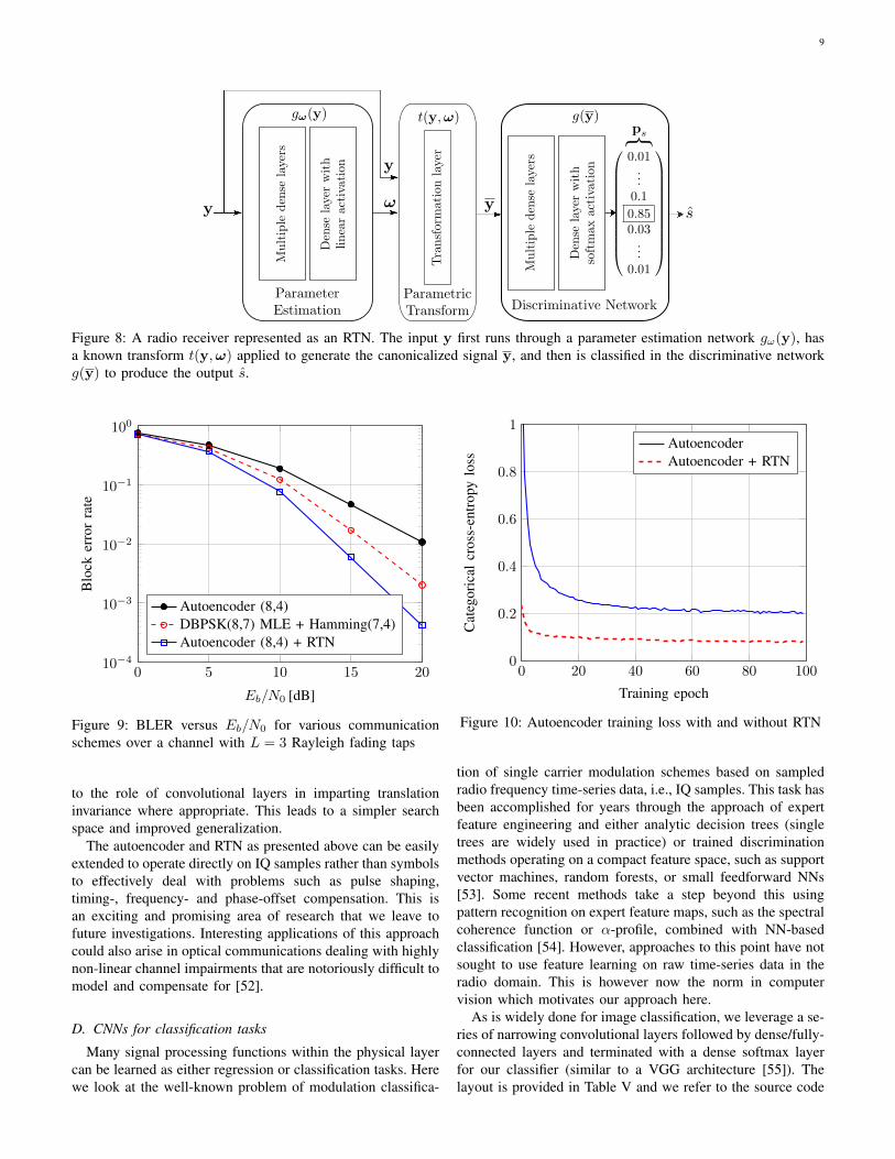
One way of augmenting DL models with expert propagationdomain knowledge but not signal specific assumptions isthrough the use of an RTN as shown in Fig. 8. An RTNconsists of three parts: (i) a learned parameter estimator gω :Rn 7→ Rp which computes a parameter vector ω ∈ Rp fromits input y, (ii) a parametric transform t : Rn×Rp 7→ Rn′ thatapplies a deterministic (and differentiable) function to y whichis parametrized by ω and suited to the propagation phenomena,and (iii) a learned discriminative network g : Rn′ 7→ M whichproduces the estimate s of the transmitted message (or otherlabel information) from the canonicalized input y ∈ Rn′ .By allowing the parameter estimator gω to take the formof an NN, we can train the system end-to-end to optimizefor a given loss function. Importantly, the training process ofsuch an RTN does not seek to directly improve the parameterestimation itself but rather optimizes the way the parametersare estimated to obtain the best end-to-end performance (e.g.,

BLER). While the example above describes an RTN forreceiver-side processing, it can similarly be used whereverparametric transformations seeded by estimated parameters areneeded. RTNs are a form of learned feed-forward attentioninspired by Spatial Transformer Networks (STNs) [51] whichhave worked well for computer vision problems.

The basic functioning of an RTN is best understood from asimple example, such as the problem of phase offset estimationand compensation. Let yc = ejϕyc ∈ Cn be a vector of IQsamples that have undergone a phase rotation by the phaseoffset ϕ, and let y = [<{y}T,={y}T]T ∈ R2n. The goalof gω is to estimate a scalar ϕ = ω = gω(y) that is closeto the phase offset ϕ, which is then used by the parametrictransform t to compute yc = e−jϕyc. The canonicalized signaly = [<{yc}T,={yc}T]T is thus given by

y = t(ϕ,y) =

[cos(ϕ)<{yc}+ sin(ϕ)={yc}cos(ϕ)={yc} − sin(ϕ)<{yc}

](11)

and then fed into the discriminative network g for furtherprocessing, such as classification.

A compelling example demonstrating the advantages ofRTNs is shown in Fig. 9 which compares the BLER of anautoencoder (8,4)7 with and without RTN over a multipathfading channel with L = 3 channel taps. That is, the receivedsignal y = [<{yc}T,={yc}T]T ∈ R2n is given as

yc,i =

L∑`=1

hc,`xc,i−`+1 + nc,i (12)

where hc ∼ CN (0, L−1IL) are i.i.d. Rayleigh fading channeltaps, nc ∼ CN (0, (REb/N0)−1In) is receiver noise, and xc ∈Cn is the transmitted signal, where we assume in (12) xc,i = 0for i ≤ 0. Here, the goal of the parameter estimator is topredict a complex-valued vector ωc (represented by 2L realvalues) that is used in the transformation layer to compute thecomplex convolution of yc with ωc. Thus, the RTN tries toequalize the channel output through inverse filtering in orderto simplify the task of the discriminative network. We haveimplemented the estimator as an NN with two dense layerswith tanh activations followed by a dense output layer withlinear activations.

While the plain autoencoder struggles to meet the perfor-mance of differential BPSK (DBPSK) with maximum likeli-hood sequence estimation (MLE) and a Hamming (7,4) code,the autoencoder with RTN outperforms it. Another advantageof RTNs is faster training convergence which can be seen fromFig. 10 that compares the validation loss of the autoencoderwith and without RTN as a function of the training epochs.We have observed in our experiments that the autoencoderwith RTN consistently outperforms the plain autoencoder,independently of the chosen hyper-parameters. However, theperformance differences diminish when the encoder and de-coder networks are made wider and trained for more iterations.Although there is theoretically nothing an RTN-augmented NNcan do that a plain NN cannot, the RTN helps by incorporatingdomain knowledge to simplify the target manifold, similar

7We assume complex-valued channel uses, so that transmitter and receiverhave 2n real-valued inputs and outputs.

9

Figure 8: A radio receiver represented as an RTN. The input y first runs through a parameter estimation network gω(y), hasa known transform t(y,ω) applied to generate the canonicalized signal y, and then is classified in the discriminative networkg(y) to produce the output s.

0 5 10 15 2010−4

10−3

10−2

10−1

100

Eb/N0 [dB]

Blo

cker

ror

rate

Autoencoder (8,4)DBPSK(8,7) MLE + Hamming(7,4)Autoencoder (8,4) + RTN

Figure 9: BLER versus Eb/N0 for various communicationschemes over a channel with L = 3 Rayleigh fading taps

to the role of convolutional layers in imparting translationinvariance where appropriate. This leads to a simpler searchspace and improved generalization.

The autoencoder and RTN as presented above can be easilyextended to operate directly on IQ samples rather than symbolsto effectively deal with problems such as pulse shaping,timing-, frequency- and phase-offset compensation. This isan exciting and promising area of research that we leave tofuture investigations. Interesting applications of this approachcould also arise in optical communications dealing with highlynon-linear channel impairments that are notoriously difficult tomodel and compensate for [52].

D. CNNs for classification tasks

Many signal processing functions within the physical layercan be learned as either regression or classification tasks. Herewe look at the well-known problem of modulation classifica-

0 20 40 60 80 1000

0.2

0.4

0.6

0.8

1

Training epoch

Cat

egor

ical

cros

s-en

trop

ylo

ss

AutoencoderAutoencoder + RTN

Figure 10: Autoencoder training loss with and without RTN

tion of single carrier modulation schemes based on sampledradio frequency time-series data, i.e., IQ samples. This task hasbeen accomplished for years through the approach of expertfeature engineering and either analytic decision trees (singletrees are widely used in practice) or trained discriminationmethods operating on a compact feature space, such as supportvector machines, random forests, or small feedforward NNs[53]. Some recent methods take a step beyond this usingpattern recognition on expert feature maps, such as the spectralcoherence function or α-profile, combined with NN-basedclassification [54]. However, approaches to this point have notsought to use feature learning on raw time-series data in theradio domain. This is however now the norm in computervision which motivates our approach here.

As is widely done for image classification, we leverage a se-ries of narrowing convolutional layers followed by dense/fully-connected layers and terminated with a dense softmax layerfor our classifier (similar to a VGG architecture [55]). Thelayout is provided in Table V and we refer to the source code

10

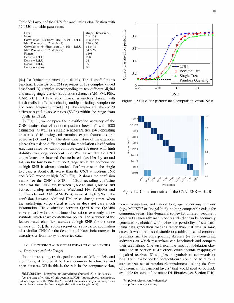
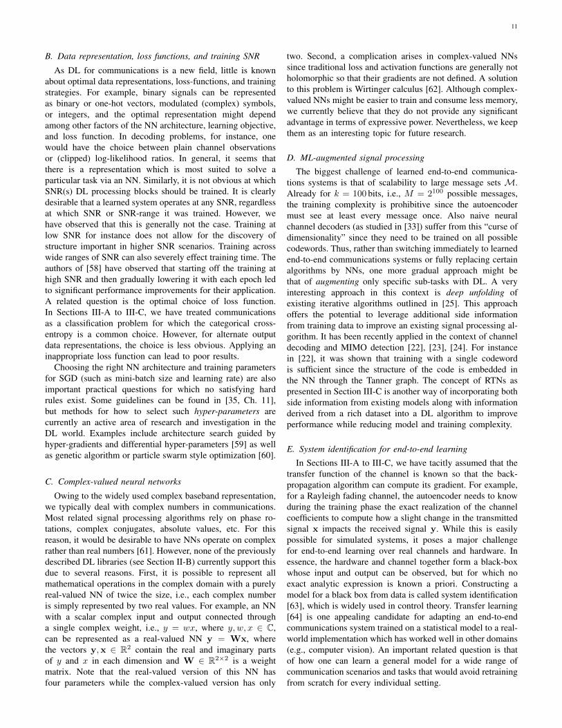
Table V: Layout of the CNN for modulation classification with324,330 trainable parameters

Layer Output dimensionsInput 2× 128Convolution (128 filters, size 2× 8) + ReLU 128× 121Max Pooling (size 2, strides 2) 128× 60Convolution (64 filters, size 1× 16) + ReLU 64× 45Max Pooling (size 2, strides 2) 64× 22Flatten 1408Dense + ReLU 128Dense + ReLU 64Dense + ReLU 32Dense + softmax 10

[44] for further implementation details. The dataset8 for thisbenchmark consists of 1.2M sequences of 128 complex-valuedbasedband IQ samples corresponding to ten different digitaland analog single-carrier modulation schemes (AM, FM, PSK,QAM, etc.) that have gone through a wireless channel withharsh realistic effects including multipath fading, sample rateand center frequency offset [31]. The samples are taken at 20different signal-to-noise ratios (SNRs) within the range from−20 dB to 18 dB.

In Fig. 11, we compare the classification accuracy of theCNN against that of extreme gradient boosting9 with 1000estimators, as well as a single scikit-learn tree [56], operatingon a mix of 16 analog and cumulant expert features as pro-posed in [53] and [57]. The short-time nature of the examplesplaces this task on difficult end of the modulation classificationspectrum since we cannot compute expert features with highstability over long periods of time. We can see that the CNNoutperforms the boosted feature-based classifier by around4 dB in the low to medium SNR range while the performanceat high SNR is almost identical. Performance in the singletree case is about 6 dB worse than the CNN at medium SNRand 3.5 % worse at high SNR. Fig. 12 shows the confusionmatrix for the CNN at SNR = 10 dB revealing confusingcases for the CNN are between QAM16 and QAM64 andbetween analog modulations Wideband FM (WBFM) anddouble-sideband AM (AM-DSB), even at high SNR. Theconfusion between AM and FM arises during times whenthe underlying voice signal is idle or does not cary muchinformation. The distinction between QAM16 and QAM64is very hard with a short-time observation over only a fewsymbols which share constellation points. The accuracy of thefeature-based classifier saturates at high SNR for the samereasons. In [58], the authors report on a successful applicationof a similar CNN for the detection of black hole mergers inastrophysics from noisy time-series data.

IV. DISCUSSION AND OPEN RESEARCH CHALLENGES

A. Data sets and challenges

In order to compare the performance of ML models andalgorithms, it is crucial to have common benchmarks andopen datasets. While this is the rule in the computer vision,

8RML2016.10b—https://radioml.com/datasets/radioml-2016-10-dataset/9At the time of writing of this document, XGB (http://xgboost.readthedocs.

io/) was together with CNNs the ML model that consistently won competionson the data-science platform Kaggle (https://www.kaggle.com/).

−20 −10 0 100

0.2

0.4

0.6

0.8

1

SNR

Cor

rect

clas

sific

atio

npr

obab

ility

CNNBoosted TreeSingle TreeRandom Guessing

Figure 11: Classifier performance comparison versus SNR

8PSK

AM-DSBBPS

KCPFS

KGFS

KPA

M4QAM16

QAM64QPS

KWBFM

Prediction

8PSK

AM-DSB

BPSK

CPFSK

GFSK

PAM4

QAM16

QAM64

QPSK

WBFM

Grou

nd tr

uth

0.0

0.2

0.4

0.6

0.8

1.0

Figure 12: Confusion matrix of the CNN (SNR = 10 dB)

voice recognition, and natural language processing domains(e.g., MNIST10 or ImageNet11), nothing comparable exists forcommunications. This domain is somewhat different because itdeals with inherently man-made signals that can be accuratelygenerated synthetically, allowing the possibility of standard-izing data generation routines rather than just data in somecases. It would be also desirable to establish a set of commonproblems and the corresponding datasets (or data-generatingsoftware) on which researchers can benchmark and comparetheir algorithms. One such example task is modulation clas-sification in Section III-D; others could include mapping ofimpaired received IQ samples or symbols to codewords orbits. Even “autoencoder competitions” could be held for astandardized set of benchmark impairments, taking the formof canonical “impairment layers” that would need to be madeavailable for some of the major DL libraries (see Section II-B).

10http://yann.lecun.com/exdb/mnist/11http://www.image-net.org/

11

B. Data representation, loss functions, and training SNR

As DL for communications is a new field, little is knownabout optimal data representations, loss-functions, and trainingstrategies. For example, binary signals can be representedas binary or one-hot vectors, modulated (complex) symbols,or integers, and the optimal representation might dependamong other factors of the NN architecture, learning objective,and loss function. In decoding problems, for instance, onewould have the choice between plain channel observationsor (clipped) log-likelihood ratios. In general, it seems thatthere is a representation which is most suited to solve aparticular task via an NN. Similarly, it is not obvious at whichSNR(s) DL processing blocks should be trained. It is clearlydesirable that a learned system operates at any SNR, regardlessat which SNR or SNR-range it was trained. However, wehave observed that this is generally not the case. Training atlow SNR for instance does not allow for the discovery ofstructure important in higher SNR scenarios. Training acrosswide ranges of SNR can also severely effect training time. Theauthors of [58] have observed that starting off the training athigh SNR and then gradually lowering it with each epoch ledto significant performance improvements for their application.A related question is the optimal choice of loss function.In Sections III-A to III-C, we have treated communicationsas a classification problem for which the categorical cross-entropy is a common choice. However, for alternate outputdata representations, the choice is less obvious. Applying aninappropriate loss function can lead to poor results.

Choosing the right NN architecture and training parametersfor SGD (such as mini-batch size and learning rate) are alsoimportant practical questions for which no satisfying hardrules exist. Some guidelines can be found in [35, Ch. 11],but methods for how to select such hyper-parameters arecurrently an active area of research and investigation in theDL world. Examples include architecture search guided byhyper-gradients and differential hyper-parameters [59] as wellas genetic algorithm or particle swarm style optimization [60].

C. Complex-valued neural networks

Owing to the widely used complex baseband representation,we typically deal with complex numbers in communications.Most related signal processing algorithms rely on phase ro-tations, complex conjugates, absolute values, etc. For thisreason, it would be desirable to have NNs operate on complexrather than real numbers [61]. However, none of the previouslydescribed DL libraries (see Section II-B) currently support thisdue to several reasons. First, it is possible to represent allmathematical operations in the complex domain with a purelyreal-valued NN of twice the size, i.e., each complex numberis simply represented by two real values. For example, an NNwith a scalar complex input and output connected througha single complex weight, i.e., y = wx, where y, w, x ∈ C,can be represented as a real-valued NN y = Wx, wherethe vectors y,x ∈ R2 contain the real and imaginary partsof y and x in each dimension and W ∈ R2×2 is a weightmatrix. Note that the real-valued version of this NN hasfour parameters while the complex-valued version has only

two. Second, a complication arises in complex-valued NNssince traditional loss and activation functions are generally notholomorphic so that their gradients are not defined. A solutionto this problem is Wirtinger calculus [62]. Although complex-valued NNs might be easier to train and consume less memory,we currently believe that they do not provide any significantadvantage in terms of expressive power. Nevertheless, we keepthem as an interesting topic for future research.

D. ML-augmented signal processing

The biggest challenge of learned end-to-end communica-tions systems is that of scalability to large message sets M.Already for k = 100 bits, i.e., M = 2100 possible messages,the training complexity is prohibitive since the autoencodermust see at least every message once. Also naive neuralchannel decoders (as studied in [33]) suffer from this “curse ofdimensionality” since they need to be trained on all possiblecodewords. Thus, rather than switching immediately to learnedend-to-end communications systems or fully replacing certainalgorithms by NNs, one more gradual approach might bethat of augmenting only specific sub-tasks with DL. A veryinteresting approach in this context is deep unfolding ofexisting iterative algorithms outlined in [25]. This approachoffers the potential to leverage additional side informationfrom training data to improve an existing signal processing al-gorithm. It has been recently applied in the context of channeldecoding and MIMO detection [22], [23], [24]. For instancein [22], it was shown that training with a single codewordis sufficient since the structure of the code is embedded inthe NN through the Tanner graph. The concept of RTNs aspresented in Section III-C is another way of incorporating bothside information from existing models along with informationderived from a rich dataset into a DL algorithm to improveperformance while reducing model and training complexity.

E. System identification for end-to-end learning

In Sections III-A to III-C, we have tacitly assumed that thetransfer function of the channel is known so that the back-propagation algorithm can compute its gradient. For example,for a Rayleigh fading channel, the autoencoder needs to knowduring the training phase the exact realization of the channelcoefficients to compute how a slight change in the transmittedsignal x impacts the received signal y. While this is easilypossible for simulated systems, it poses a major challengefor end-to-end learning over real channels and hardware. Inessence, the hardware and channel together form a black-boxwhose input and output can be observed, but for which noexact analytic expression is known a priori. Constructing amodel for a black box from data is called system identification[63], which is widely used in control theory. Transfer learning[64] is one appealing candidate for adapting an end-to-endcommunications system trained on a statistical model to a real-world implementation which has worked well in other domains(e.g., computer vision). An important related question is thatof how one can learn a general model for a wide range ofcommunication scenarios and tasks that would avoid retrainingfrom scratch for every individual setting.

12

F. Learning from CSI and beyond

Accurate channel state information (CSI) is a fundamentalrequirement for multi-user MIMO communications. For thisreason, current cellular communication systems invest signif-icant resources (energy and time) in the acquisition of CSIat the base station and user equipment. This information isgenerally not used for anything apart from precoding/detectionor other tasks directly related to processing of the current dataframe. Storing and analyzing large amounts of CSI (or otherradio data)—possibly enriched with location information—poses significant potential for revealing novel big-data-drivenphysical-layer understanding algorithms beyond immidiate ra-dio environment needs. New applications beyond the tradi-tional scope of communications, such as tracking and iden-tification of humans (through walls) [65] as well as gestureand emotion recognition [66], could be achieved using ML onradio signals.

V. CONCLUSION

We have discussed several promising new applications ofDL to the physical layer. Most importantly, we have introduceda new way of thinking about communications as an end-to-endreconstruction optimization task using autoencoders to jointlylearn transmitter and receiver implementations as well assignal encodings without any prior knowledge. Comparisonswith traditional baselines in various scenarios reveal extremelycompetitive BLER performance, although the scalability tolong block lengths remains a challenge. Apart from potentialperformance improvements in terms of reliability or latency,our approach can provide interesting insight about the opti-mal communication schemes (e.g., constellations) in scenarioswhere the optimal schemes are unknown (e.g., interferencechannel). We believe that this is the beginning of a widerange of studies into DL and ML for communications andare excited at the possibilities this could lend towards futurewireless communications systems as the field matures. Fornow, there are a great number of open problems to solveand practical gains to be had. We have identified importantkey areas of future investigation and highlighted the need forbenchmark problems and data sets that can be used to compareperformance of different ML models and algorithms.

REFERENCES

[1] T. S. Rappaport, Wireless communications: Principles and practice,2nd ed. Prentice Hall, 2002.

[2] R. M. Gagliardi and S. Karp, Optical communications, 2nd ed. Wiley,1995.

[3] H. Meyr, M. Moeneclaey, and S. A. Fechtel, Digital communicationreceivers: Synchronization, channel estimation, and signal processing.John Wiley & Sons, Inc., 1998.

[4] T. Schenk, RF imperfections in high-rate wireless systems: Impact anddigital compensation. Springer Science & Business Media, 2008.

[5] J. Proakis and M. Salehi, Digital Communications, 5th ed. McGraw-Hill Education, 2007.

[6] Y. LeCun et al., “Generalization and network design strategies,” Con-nectionism in perspective, pp. 143–155, 1989.

[7] K. He, X. Zhang, S. Ren, and J. Sun, “Delving deep into rectifiers:Surpassing human-level performance on imagenet classification,” inProc. IEEE Int. Conf. Computer Vision, 2015, pp. 1026–1034.

[8] D. G. Lowe, “Object recognition from local scale-invariant features,” inProc. IEEE Int. Conf. Computer Vision, 1999, pp. 1150–1157.

[9] Z. S. Harris, “Distributional structure,” Word, vol. 10, no. 2-3, pp. 146–162, 1954.

[10] A. Goldsmith, “Joint source/channel coding for wireless channels,” inProc. IEEE Vehicular Technol. Conf., vol. 2, 1995, pp. 614–618.

[11] E. Zehavi, “8-PSK trellis codes for a Rayleigh channel,” IEEE Trans.Commun., vol. 40, no. 5, pp. 873–884, 1992.

[12] H. Wymeersch, Iterative receiver design. Cambridge University Press,2007, vol. 234.

[13] K. Hornik, M. Stinchcombe, and H. White, “Multilayer feedforwardnetworks are universal approximators,” Neural networks, vol. 2, no. 5,pp. 359–366, 1989.

[14] S. Reed and N. de Freitas, “Neural programmer-interpreters,” arXivpreprint arXiv:1511.06279, 2015.

[15] H. T. Siegelmann and E. D. Sontag, “On the computational power ofneural nets,” in Proc. 5th Annu. Workshop Computational LearningTheory. ACM, 1992, pp. 440–449.

[16] V. Vanhoucke, A. Senior, and M. Z. Mao, “Improving the speed of neuralnetworks on CPUs,” in Proc. Deep Learning and Unsupervised FeatureLearning NIPS Workshop, 2011.

[17] Y.-H. Chen, T. Krishna, J. S. Emer, and V. Sze, “Eyeriss: An energy-efficient reconfigurable accelerator for deep convolutional neural net-works,” IEEE J. Solid-State Circuits, vol. 52, no. 1, pp. 127–138, 2017.

[18] R. Raina, A. Madhavan, and A. Y. Ng, “Large-scale deep unsupervisedlearning using graphics processors,” in Proc. Int. Conf. Mach. Learn.(ICML). ACM, 2009, pp. 873–880.

[19] M. Ibnkahla, “Applications of neural networks to digitalcommunications–A survey,” Elsevier Signal Processing, vol. 80,no. 7, pp. 1185–1215, 2000.

[20] M. Bkassiny, Y. Li, and S. K. Jayaweera, “A survey on machine-learningtechniques in cognitive radios,” IEEE Commun. Surveys Tuts., vol. 15,no. 3, pp. 1136–1159, 2013.

[21] J. Qadir, K.-L. A. Yau, M. A. Imran, Q. Ni, and A. V. Vasilakos,“IEEE Access Special Section Editorial: Artificial Intelligence EnabledNetworking,” IEEE Access, vol. 3, pp. 3079–3082, 2015.

[22] E. Nachmani, Y. Be’ery, and D. Burshtein, “Learning to decode linearcodes using deep learning,” in Proc. IEEE Annu. Allerton Conf. Com-mun., Control, and Computing (Allerton), 2016, pp. 341–346.

[23] E. Nachmani, E. Marciano, D. Burshtein, and Y. Be’ery, “RNN decodingof linear block codes,” arXiv preprint arXiv:1702.07560, 2017.

[24] N. Samuel, T. Diskin, and A. Wiesel, “Deep MIMO detection,” arXivpreprint arXiv:1706.01151, 2017.

[25] J. R. Hershey, J. L. Roux, and F. Weninger, “Deep unfolding:Model-based inspiration of novel deep architectures,” arXiv preprintarXiv:1409.2574, 2014.

[26] M. Borgerding and P. Schniter, “Onsager-corrected deep learning forsparse linear inverse problems,” arXiv preprint arXiv:1607.05966, 2016.

[27] Y.-S. Jeon, S.-N. Hong, and N. Lee, “Blind detection for MIMO systemswith low-resolution ADCs using supervised learning,” arXiv preprintarXiv:1610.07693, 2016.

[28] N. Farsad and A. Goldsmith, “Detection algorithms for communicationsystems using deep learning,” arXiv preprint arXiv:1705.08044, 2017.

[29] H. Sun, X. Chen, Q. Shi, M. Hong, X. Fu, and N. D. Sidiropoulos,“Learning to optimize: Training deep neural networks for wirelessresource management,” arXiv preprint arXiv:1705.09412, 2017.

[30] T. J. O’Shea, K. Karra, and T. C. Clancy, “Learning to communicate:Channel auto-encoders, domain specific regularizers, and attention,” inProc. IEEE Int. Symp. Signal Process. and Inf. Technol. (ISSPIT), 2016,pp. 223–228.

[31] T. J. O’Shea, J. Corgan, and T. C. Clancy, “Convolutional radio mod-ulation recognition networks,” in Proc. Int. Conf. Eng. Applications ofNeural Networks. Springer, 2016, pp. 213–226.

[32] T. J. O’Shea, J. Corgan, and T. C. Clancy, “Unsupervised representationlearning of structured radio communication signals,” in Proc. IEEE Int.Workshop Sensing, Processing and Learning for Intelligent Machines(SPLINE), 2016, pp. 1–5.

[33] T. Gruber, S. Cammerer, J. Hoydis, and S. ten Brink, “On deep learning-based channel decoding,” in Proc. IEEE 51st Annu. Conf. Inf. SciencesSyst. (CISS), 2017, pp. 1–6.

[34] S. Cammerer, T. Gruber, J. Hoydis, and S. t. Brink, “Scaling deeplearning-based decoding of polar codes via partitioning,” arXiv preprintarXiv:1702.06901, 2017.

[35] I. Goodfellow, Y. Bengio, and A. Courville, Deep Learning. MIT Press,2016.

[36] N. Srivastava, G. E. Hinton, A. Krizhevsky, I. Sutskever, andR. Salakhutdinov, “Dropout: A simple way to prevent neural networksfrom overfitting.” J. Mach. Learn. Res., vol. 15, no. 1, pp. 1929–1958,2014.

13

[37] V. Nair and G. E. Hinton, “Rectified linear units improve restrictedboltzmann machines,” in Proc. Int. Conf. Mach. Learn. (ICML), 2010,pp. 807–814.

[38] Y. Jia, E. Shelhamer, J. Donahue, S. Karayev, J. Long, R. Girshick,S. Guadarrama, and T. Darrell, “Caffe: Convolutional architecture forfast feature embedding,” arXiv preprint arXiv:1408.5093, 2014.

[39] T. Chen, M. Li, Y. Li, M. Lin, N. Wang, M. Wang, T. Xiao, B. Xu,C. Zhang, and Z. Zhang, “MXNet: A flexible and efficient machinelearning library for heterogeneous distributed systems,” arXiv preprintarXiv:1512.01274, 2015.

[40] M. Abadi et al., “TensorFlow: Large-scale machine learning onheterogeneous systems,” 2015, software available from tensorflow.org.[Online]. Available: http://tensorflow.org/

[41] R. Al-Rfou, G. Alain, A. Almahairi et al., “Theano: A Python frame-work for fast computation of mathematical expressions,” arXiv preprintarXiv:1605.02688, 2016.

[42] R. Collobert, K. Kavukcuoglu, and C. Farabet, “Torch7: A matlab-likeenvironment for machine learning,” in BigLearn, NIPS Workshop, 2011.

[43] F. Chollet, “keras,” https://github.com/fchollet/keras, 2015.[44] T. O’Shea and J. Hoydis, “Source code,” https://github.com/

-available-after-review, 2017.[45] G. E. Hinton, S. Osindero, and Y.-W. Teh, “A fast learning algorithm for

deep belief nets,” Neural computation, vol. 18, no. 7, pp. 1527–1554,2006.

[46] D. Kingma and J. Ba, “Adam: A method for stochastic optimization,”arXiv preprint arXiv:1412.6980, 2014.

[47] Y. N. Dauphin, R. Pascanu, C. Gulcehre, K. Cho, S. Ganguli, andY. Bengio, “Identifying and attacking the saddle point problem inhigh-dimensional non-convex optimization,” in Advances in NeuralInformation Processing Systems (NIPS), 2014, pp. 2933–2941.

[48] L. v. d. Maaten and G. Hinton, “Visualizing data using t-SNE,” J. Mach.Learn. Res., vol. 9, no. Nov, pp. 2579–2605, 2008.

[49] I. Goodfellow, J. Pouget-Abadie, M. Mirza, B. Xu, D. Warde-Farley,S. Ozair, A. Courville, and Y. Bengio, “Generative adversarial nets,” inAdvances in Neural Information Processing Systems (NIPS), 2014, pp.2672–2680.

[50] M. Abadi and D. G. Andersen, “Learning to protect communicationswith adversarial neural cryptography,” arXiv preprint arXiv:1610.06918,2016.

[51] M. Jaderberg, K. Simonyan, A. Zisserman et al., “Spatial transformernetworks,” in Advances in Neural Information Processing Systems(NIPS), 2015, pp. 2017–2025.

[52] J. Estaran et al., “Artificial neural networks for linear and non-linearimpairment mitigation in high-baudrate IM/DD systems,” in Proc. 42ndEuropean Conf. Optical Commun. (ECOC). VDE, 2016, pp. 1–3.

[53] A. K. Nandi and E. E. Azzouz, “Algorithms for automatic modulationrecognition of communication signals,” IEEE Trans. Commun., vol. 46,no. 4, pp. 431–436, 1998.

[54] A. Fehske, J. Gaeddert, and J. H. Reed, “A new approach to signal clas-sification using spectral correlation and neural networks,” in IEEE Int.Symp. New Frontiers in Dynamic Spectrum Access Networks (DYSPAN),2005, pp. 144–150.

[55] K. Simonyan and A. Zisserman, “Very deep convolutional networks forlarge-scale image recognition,” arXiv preprint arXiv:1409.1556, 2014.

[56] F. Pedregosa et al., “Scikit-learn: Machine learning in Python,” J. Mach.Learn. Res., vol. 12, pp. 2825–2830, 2011.

[57] A. Abdelmutalab, K. Assaleh, and M. El-Tarhuni, “Automatic mod-ulation classification based on high order cumulants and hierarchicalpolynomial classifiers,” Physical Communication, vol. 21, pp. 10–18,2016.

[58] D. George and E. Huerta, “Deep neural networks to enable real-timemultimessenger astrophysics,” arXiv preprint arXiv:1701.00008, 2016.

[59] D. Maclaurin, D. Duvenaud, and R. P. Adams, “Gradient-based hyper-parameter optimization through reversible learning,” in Proc. 32nd Int.Conf. Mach. Learn. (ICML), 2015.

[60] J. Bergstra and Y. Bengio, “Random search for hyper-parameter opti-mization,” J. Mach. Learn. Res., vol. 13, pp. 281–305, Feb. 2012.

[61] A. Hirose, Complex-valued neural networks. Springer Science &Business Media, 2006.

[62] M. F. Amin, M. I. Amin, A. Al-Nuaimi, and K. Murase, “Wirtingercalculus based gradient descent and Levenberg-Marquardt learning al-gorithms in complex-valued neural networks,” in Int. Conf. on NeuralInformation Processing. Springer, 2011, pp. 550–559.

[63] G. C. Goodwin and R. L. Payne, Dynamic system identification: exper-iment design and data analysis. Academic press, 1977.

[64] S. J. Pan and Q. Yang, “A survey on transfer learning,” IEEE Trans.Knowl. Data Eng., vol. 22, no. 10, pp. 1345–1359, 2010.

[65] F. Adib, C.-Y. Hsu, H. Mao, D. Katabi, and F. Durand, “Capturing thehuman figure through a wall,” ACM Trans. Graphics (TOG), vol. 34,no. 6, p. 219, 2015.

[66] M. Zhao, F. Adib, and D. Katabi, “Emotion recognition using wirelesssignals,” in Proc. ACM Annu. Int. Conf. Mobile Computing and Net-working, 2016, pp. 95–108.