An Introduction to Bayesian Hypothesis Testing for ...scheibehenne.de/AndraszewiczScheibehenneEtAl.2015.pdf · Andraszewicz et al. / Bayesian Hypothesis Testing 523 Bayesian Inference

Journal of ManagementVol. 41 No. 2, February 2015 521 –543

DOI: 10.1177/0149206314560412© The Author(s) 2014

Reprints and permissions:sagepub.com/journalsPermissions.nav

521

An Introduction to Bayesian Hypothesis Testing for Management Research

Sandra AndraszewiczUniversity of Basel

Swiss Federal Institute of Technology Zurich

Benjamin ScheibehenneJörg Rieskamp

University of Basel

Raoul GrasmanJosine Verhagen

Eric-Jan WagenmakersUniversity of Amsterdam

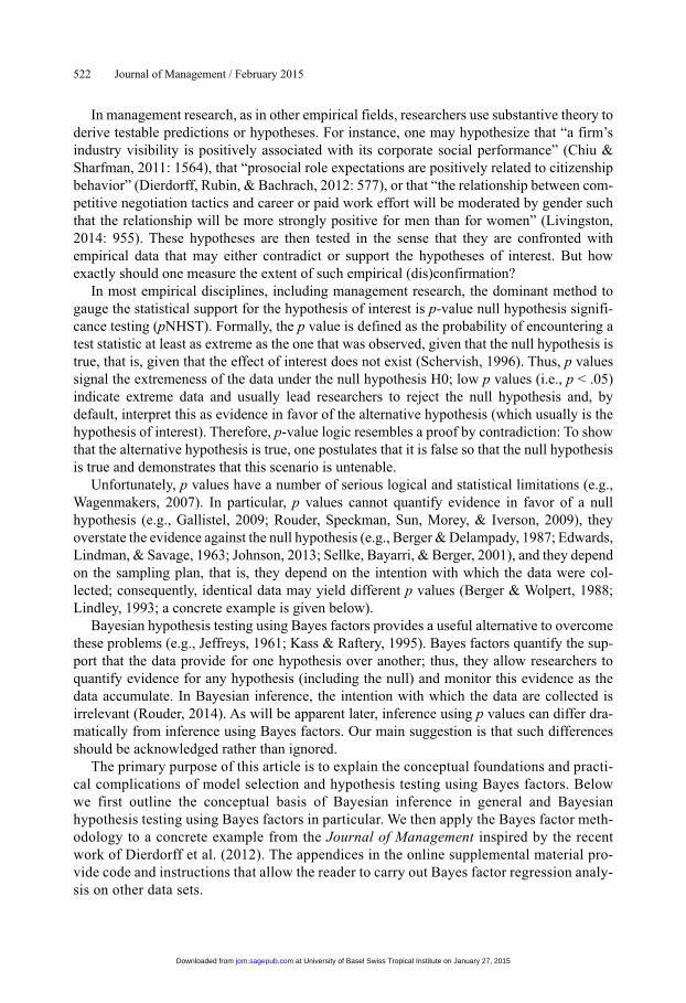
In management research, empirical data are often analyzed using p-value null hypothesis sig-nificance testing (pNHST). Here we outline the conceptual and practical advantages of an alternative analysis method: Bayesian hypothesis testing and model selection using the Bayes factor. In contrast to pNHST, Bayes factors allow researchers to quantify evidence in favor of the null hypothesis. Also, Bayes factors do not require adjustment for the intention with which the data were collected. The use of Bayes factors is demonstrated through an extended example for hierarchical regression based on the design of an experiment recently published in the Journal of Management. This example also highlights the fact that p values overestimate the evidence against the null hypothesis, misleading researchers into believing that their findings are more reliable than is warranted by the data.

Keywords: Bayes factor; statistical evidence; optional stopping

Acknowledgments: We would like to thank Jeffrey Rouder for his valuable comments and suggestions that have significantly improved the quality of this article.

Supplemental material for this article is available at http://jom.sagepub.com/supplemental

Corresponding author: Sandra Andraszewicz, Swiss Federal Institute of Technology Zurich, Clausiusstrasse 50, 8092 Zürich, Switzerland.

E-mail: [email protected]

560412 JOMXXX10.1177/0149206314560412Journal of ManagementAndraszewicz et al. / Bayesian Hypothesis Testingresearch-article2014

Special Issue: Bayesian Probability and Statistics in Management Research

at University of Basel Swiss Tropical Institute on January 27, 2015jom.sagepub.comDownloaded from

mailto:[email protected]

http://jom.sagepub.com/

522 Journal of Management / February 2015

In management research, as in other empirical fields, researchers use substantive theory to derive testable predictions or hypotheses. For instance, one may hypothesize that “a firm’s industry visibility is positively associated with its corporate social performance” (Chiu & Sharfman, 2011: 1564), that “prosocial role expectations are positively related to citizenship behavior” (Dierdorff, Rubin, & Bachrach, 2012: 577), or that “the relationship between com-petitive negotiation tactics and career or paid work effort will be moderated by gender such that the relationship will be more strongly positive for men than for women” (Livingston, 2014: 955). These hypotheses are then tested in the sense that they are confronted with empirical data that may either contradict or support the hypotheses of interest. But how exactly should one measure the extent of such empirical (dis)confirmation?

In most empirical disciplines, including management research, the dominant method to gauge the statistical support for the hypothesis of interest is p-value null hypothesis signifi-cance testing (pNHST). Formally, the p value is defined as the probability of encountering a test statistic at least as extreme as the one that was observed, given that the null hypothesis is true, that is, given that the effect of interest does not exist (Schervish, 1996). Thus, p values signal the extremeness of the data under the null hypothesis H0; low p values (i.e., p < .05) indicate extreme data and usually lead researchers to reject the null hypothesis and, by default, interpret this as evidence in favor of the alternative hypothesis (which usually is the hypothesis of interest). Therefore, p-value logic resembles a proof by contradiction: To show that the alternative hypothesis is true, one postulates that it is false so that the null hypothesis is true and demonstrates that this scenario is untenable.

Unfortunately, p values have a number of serious logical and statistical limitations (e.g., Wagenmakers, 2007). In particular, p values cannot quantify evidence in favor of a null hypothesis (e.g., Gallistel, 2009; Rouder, Speckman, Sun, Morey, & Iverson, 2009), they overstate the evidence against the null hypothesis (e.g., Berger & Delampady, 1987; Edwards, Lindman, & Savage, 1963; Johnson, 2013; Sellke, Bayarri, & Berger, 2001), and they depend on the sampling plan, that is, they depend on the intention with which the data were col-lected; consequently, identical data may yield different p values (Berger & Wolpert, 1988; Lindley, 1993; a concrete example is given below).

Bayesian hypothesis testing using Bayes factors provides a useful alternative to overcome these problems (e.g., Jeffreys, 1961; Kass & Raftery, 1995). Bayes factors quantify the sup-port that the data provide for one hypothesis over another; thus, they allow researchers to quantify evidence for any hypothesis (including the null) and monitor this evidence as the data accumulate. In Bayesian inference, the intention with which the data are collected is irrelevant (Rouder, 2014). As will be apparent later, inference using p values can differ dra-matically from inference using Bayes factors. Our main suggestion is that such differences should be acknowledged rather than ignored.

The primary purpose of this article is to explain the conceptual foundations and practi-cal complications of model selection and hypothesis testing using Bayes factors. Below we first outline the conceptual basis of Bayesian inference in general and Bayesian hypothesis testing using Bayes factors in particular. We then apply the Bayes factor meth-odology to a concrete example from the Journal of Management inspired by the recent work of Dierdorff et al. (2012). The appendices in the online supplemental material pro-vide code and instructions that allow the reader to carry out Bayes factor regression analy-sis on other data sets.



Andraszewicz et al. / Bayesian Hypothesis Testing 523

Bayesian Inference in a Nutshell

The methodology of p values is based on frequentist statistics, in which probability is conceptualized as the proportion of occurrences in the large-sample limit. An alternative statistical paradigm, whose popularity has risen tremendously over the past 20 years (e.g., Poirier, 2006), is Bayesian inference. In Bayesian inference, probability is used to quantify uncertainty or degree of belief.

The many aspects of Bayesian inference are explained in detail elsewhere (e.g., Dienes, 2008; Kruschke, 2010; M. D. Lee & Wagenmakers, 2013; and the articles in this special issue, such as Zyphur & Oswald, 2015). Here we explain the essentials in as far as they are required to understand, at a conceptual level, the material covered in later sections.

As a concrete example, consider Study 3 from Bechtoldt, de Dreu, Nijstad, and Zapf (2010), in which a sample of 75 midlevel employees from a large health insurance company in The Netherlands were asked to complete the Dutch Test for Conflict Handling (DUTCH; de Dreu, Evers, Beersma, Kluwer, & Nauta, 2001). This test measures the extent to which an employee self-identifies with four different styles of conflict management (i.e., problem solving, contending, avoiding, and yielding). The DUTCH measures each conflict manage-ment strategy using four items on a scale from 1 (strongly disagree) to 5 (strongly agree). Sample items are “I give in to the wishes of the other party” (yielding) or “I avoid a confron-tation about our differences” (avoiding).

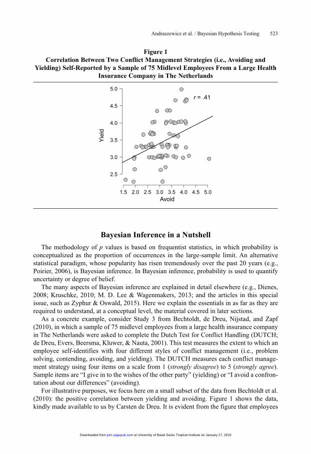
For illustrative purposes, we focus here on a small subset of the data from Bechtoldt et al. (2010): the positive correlation between yielding and avoiding. Figure 1 shows the data, kindly made available to us by Carsten de Dreu. It is evident from the figure that employees

Figure 1Correlation Between Two Conflict Management Strategies (i.e., Avoiding and

Yielding) Self-Reported by a Sample of 75 Midlevel Employees From a Large Health Insurance Company in The Netherlands

1.5 2.0 2.5 3.0 3.5 4.0 4.5 5.0

2.5

3.0

3.5

4.0

4.5

5.0

Avoid

Yiel

dr = .41




with high scores on yielding also tend to have high scores on avoiding. This relation can be quantified by the Pearson correlation coefficient, whose sample value (r) equals .41 and is significantly different from 0 (p = .0003, two-sided test; Table 4 in Bechtoldt et al.).

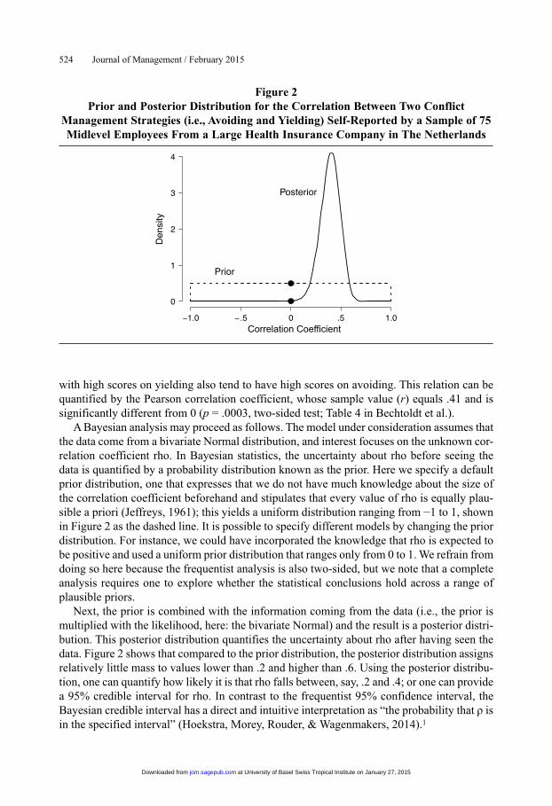
A Bayesian analysis may proceed as follows. The model under consideration assumes that the data come from a bivariate Normal distribution, and interest focuses on the unknown cor-relation coefficient rho. In Bayesian statistics, the uncertainty about rho before seeing the data is quantified by a probability distribution known as the prior. Here we specify a default prior distribution, one that expresses that we do not have much knowledge about the size of the correlation coefficient beforehand and stipulates that every value of rho is equally plau-sible a priori (Jeffreys, 1961); this yields a uniform distribution ranging from −1 to 1, shown in Figure 2 as the dashed line. It is possible to specify different models by changing the prior distribution. For instance, we could have incorporated the knowledge that rho is expected to be positive and used a uniform prior distribution that ranges only from 0 to 1. We refrain from doing so here because the frequentist analysis is also two-sided, but we note that a complete analysis requires one to explore whether the statistical conclusions hold across a range of plausible priors.

Next, the prior is combined with the information coming from the data (i.e., the prior is multiplied with the likelihood, here: the bivariate Normal) and the result is a posterior distri-bution. This posterior distribution quantifies the uncertainty about rho after having seen the data. Figure 2 shows that compared to the prior distribution, the posterior distribution assigns relatively little mass to values lower than .2 and higher than .6. Using the posterior distribu-tion, one can quantify how likely it is that rho falls between, say, .2 and .4; or one can provide a 95% credible interval for rho. In contrast to the frequentist 95% confidence interval, the Bayesian credible interval has a direct and intuitive interpretation as “the probability that ρ is in the specified interval” (Hoekstra, Morey, Rouder, & Wagenmakers, 2014).1

Figure 2Prior and Posterior Distribution for the Correlation Between Two Conflict

Management Strategies (i.e., Avoiding and Yielding) Self-Reported by a Sample of 75 Midlevel Employees From a Large Health Insurance Company in The Netherlands

Correlation Coefficient




Bayesian Hypothesis Testing

The posterior distribution allows one to answer the general question, what do we know about the correlation between yielding and avoiding in the Dutch employees, assuming from the outset that such a correlation exists? This formulation reveals that we cannot use the posterior distribution alone for drawing conclusions about competing hypotheses because doing so presupposes that the null hypothesis is false. Consequently, hypothesis testing based on forming a confidence region for the parameter of interest can be misleading (Berger, 2006: 383).

Hence, when the goal is hypothesis testing, Bayesians need to go beyond the posterior distribution. To answer the question regarding to what extent the data support the presence of a correlation, one needs to compare two models: a null hypothesis that states the absence of the effect (i.e., H0: ρ = 0) and an alternative hypothesis that states its presence. In Bayesian statistics, this alternative hypothesis needs to be specified precisely. In our scenario, the alter-native hypothesis is specified as H1: ρ ~ Uniform(−1,1), that is, rho is distributed uniformly ranging from −1 to 1 (i.e., before seeing the data, every value of rho is deemed equally likely).

In Bayesian hypothesis testing, hypotheses or models may be more or less plausible a priori.2 Before having seen the data, the relative plausibility of the competing models can be expressed through the prior model odds, that is, p(H1)/p(H0). These prior model odds quan-tify a researcher’s skepticism towards H1 on the basis of theoretical considerations and gen-eral knowledge of the world. Thus, when H1 is relatively implausible (e.g., to us: people can look into the future; neutrinos travel faster than the speed of light; people are more creative in the presence of a big box), this translates into low prior odds that H1 is true. Recall that, in the Bayesian paradigm, both p(H1) and p(H0) indicate degree of belief and are used to quan-tify uncertainty. A frequentist may insist that H0 is either true or false, and that, therefore, it cannot have a probability. The Bayesian reply is that the “p” in p(H0) does not represent a proportion in a large-sample limit but, instead, represents the degree of belief we are willing to assign to H0 on the basis of our current knowledge of the world.

After having seen the data D, the relative plausibility is known as the posterior model odds, that is, p(H1 | D)/p(H0 | D). The change from prior to posterior odds that is brought about by the data is referred to as the Bayes factor, that is, BF10 = p(D | H1)/p(D | H0). Thus, the Bayes factor grades the decisiveness of the evidence by pitting against each other the probability of the observed data under H1 versus the probability of the observed data under H0. When H1 is defined as a single point (i.e., ρ = .4), the Bayes factor reduces to a simple likelihood ratio.

Because of the inherently subjective nature of the prior model odds, the emphasis of Bayesian hypothesis testing is on the amount by which the data shift one’s beliefs, that is, on the Bayes factor. Thus, when the Bayes factor BF10 equals 10.5, the data are 10.5 times more likely under H1 than under H0. When the Bayes factor BF10 equals 0.2, the data are 5 times more likely under H0 than under H1. This way, the Bayes factor offers a method for skeptics and proponents to agree on the evidence provided by the data, while still disagreeing on the prior odds (and, hence, the posterior odds). Consider an extreme example: A psi proponent might believe it is entirely reasonable that people can look into the future, whereas a psi skeptic might believe that this is virtually impossible. Hence, their prior odds on the exis-tence of psi differ greatly. Nevertheless, the proponent and skeptic may fully agree on the




extent to which the data from a particular experiment change the prior odds. As more data become available, both skeptic and proponent should adjust their beliefs in the direction of the hypothesis that is best supported by the data. A spatial analogy is that the Bayes factor measures neither the starting point of a journey nor the end point; instead, it measures the distance that is traveled.

Even though the Bayes factor has an unambiguous and continuous scale, it is sometimes useful to summarize the Bayes factor in terms of discrete categories of evidential strength. Jeffreys (1961, Appendix B) proposed the classification scheme shown in Table 1. We replaced the labels “worth no more than a bare mention” with “anecdotal,” “substantial” with “moderate,” and “decisive” with “extreme” (Wetzels, van Ravenzwaaij, & Wagenmakers, in press). These labels facilitate scientific communication but should be considered only as an approximate descriptive articulation of different standards of evidence.

Bayes factors represent “the standard Bayesian solution to the hypothesis testing and model selection problems” (Lewis & Raftery, 1997: 648) and “the primary tool used in Bayesian inference for hypothesis testing and model selection” (Berger, 2006: 378). Nevertheless, Bayes factors come with a series of challenges, three of which stand out. These challenges are discussed in the next section, which may be skipped by the reader who is not interested in the statistical details.

Three Challenges for Bayesian Hypothesis Testing

The first challenge for Bayesian hypothesis testing is the specification of sensible prior distributions for the parameters that are subject to test. For Bayesian hypothesis testing, it matters whether we test H0 versus H1: ρ ~ Uniform(–1,1) (the correlation can take on any value), versus H2: ρ ~ Uniform(0,1) (the correlation is positive), or versus, say, H3: ρ ~ Uniform(–0.1, 0.1) (there is a correlation but it is small). The fact that the result depends on the prior specification is not in itself a challenge or a limitation. In fact, it is desirable that different results are obtained for different models: H1 is a relatively flexible model that keeps all options open, and H2 is less flexible than H1 because it rules out the possibility that rho is negative. Finally, H3 is the most parsimonious, least flexible alternative model—it is very

Table 1

Evidence Categories for the Bayes Factor BF12 (Adjusted From Jeffreys, 1961)

Bayes factor BF12 Interpretation

> 100 Extreme evidence for M1

30 — 100 Very strong evidence for M1

10 — 30 Strong evidence for M1

3 — 10 Moderate evidence for M1

1 — 3 Anecdotal evidence for M1

1 No evidence1/3 — 1 Anecdotal evidence for M2

1/10 — 1/3 Moderate evidence for M2

1/30 — 1/10 Strong evidence for M2

1/100 — 1/30 Very strong evidence for M2

< 1/100 Extreme evidence for M2




similar, in fact, to H0 and therefore a relatively large number of data points will be required before H3 can be discriminated from H0 with much confidence. It should be noted that this claim is not undisputed, and some statisticians prefer a method for hypothesis testing or model selection that is less sensitive to prior specification (for a discussion, see Aitkin, 1991; Liu & Aitkin, 2008; Vanpaemel, 2010).

Because the Bayesian hypothesis test is relatively sensitive—as it should be—to the prior distribution, the specification of this prior distribution requires considerable care. In the case of the Pearson correlation, we may follow Jeffreys (1961) and place a uniform prior on rho, but this is not feasible for variables with unbounded support, such as the mean of a Normal distribution. Considerable effort has been spent to develop “default” prior distributions, that is, prior distributions that work well across a wide range of substantively different applica-tions. For instance, the default priors we use for linear regression are known as the Jeffreys-Zellner-Siow (JZS) priors (Jeffreys; Liang, Paulo, Molina, Clyde, & Berger, 2008; Rouder & Morey, 2012; Zellner & Siow, 1980); as discussed later, these priors fulfill several general desiderata and can provide a reference analysis that may, if needed, be fine-tuned using problem-specific information.

Another less obvious manifestation of the first challenge relates to the specification of the null hypothesis. Traditionally, in frequentist and Bayesian frameworks alike, the null hypoth-esis is specified as a single point, in this case, H0: ρ = 0. However, it has been argued that, in observational studies at least, the null hypothesis is never true exactly (e.g., Cohen, 1994; Meehl, 1978). When this is the case, the conclusion is already known before the experiment is conducted: “the null hypothesis is false.” All that needs to happen to make the test support this truism is to collect a sufficient number of observations. From this perspective, a test of a point null hypothesis is merely a check on whether the number of observations was large enough.

In the interest of brevity, we forgo a philosophical debate on the circumstances under which a point null hypothesis can be true exactly. Instead, the principled Bayesian solution to the problem—when it is felt to be particularly acute—is to change the specification of the null hypothesis from a single point to a small interval around 0 (Morey & Rouder, 2011). In the case of the conflict management strategy example above, such an interval null hypothesis can be specified, for example, as H0: ρ ~ Uniform(–.05,.05), a uniform distribu-tion from –.05 to .05. Thus, Bayes factors can be used to test a wide variety of different models; when there are compelling a priori reasons to question the relevance of a point null hypothesis, the Bayesian framework allows the researcher to specify and test a null hypoth-esis instead.

It is worth stressing that, as in all modeling of the hypothesis-testing type, the crucial ele-ments of the model specification need to be in place before the data have been observed (e.g., De Groot 1956/2014). If this rule is violated, a researcher runs the danger of using the data twice: once to motivate or fine-tune the hypothesis and again to test that hypothesis. Such double use of data is not allowed in any statistical paradigm, be it frequentist or Bayesian.

The second challenge for Bayesian hypothesis testing is whether hypothesis testing should be engaged in at all. Several statisticians and social scientists have argued that testing should be replaced by estimation (e.g., Cumming, 2014; Gelman & Rubin, 1995; Kruschke, 2010). This debate might never be settled, but it is our belief that hypothesis testing constitutes a legitimate scientific endeavor that requires a proper statistical implementation (Morey, Rouder, Verhagen, & Wagenmakers, 2014). For instance, suppose a team of researchers




wishes to study whether the consumption of red wine helps prevent the common cold (Takkouche, Regueira-Mendez, Garcia-Closas, Figueiras, Gestal-Otero, & Hernan, 2002). After the data have been collected, the immediate, intuitive, and legitimate scientific ques-tion is, does the consumption of red wine help prevent the common cold or does it not? If there is any beneficial effect at all, even if it is small, then follow-up research may be called for. Such follow-up research may seek to understand the putative biological mechanism and thereby open up avenues to amplify or adjust the effect. Note that there exists only one spe-cial effect size that can never be amplified, no matter how delicate the purification of the materials and design. This unique effect size is 0. In other words, the presence of an effect is qualitatively different from the absence of an effect. Can people look into the future? Is a particular gene involved in the progression of Alzheimer’s? Did researchers observe the Higgs boson? Can neutrinos travel faster than the speed of light? All of these questions are legitimate, and yet an estimation framework is unsuited to address them. Of course, estima-tion fulfills an important scientific function; after confirming that there is an effect, the very next question is, How big is it? Effect size estimation fulfills an important role, which is most clearly seen in prediction and in cost-benefit analyses. But before estimating the size of an effect, we first need to estimate whether it is present at all. This sentiment echoes that of Sir Harold Jeffreys: “If K [the Bayes factor] is small, so that the null hypothesis has a small prob-ability, we shall want an estimate of α [the parameter under scrutiny] on the alternative hypothesis” (1973: 55).

The third and final challenge for Bayesian hypothesis testing is computational: Bayes factors can be relatively difficult to obtain. The Bayes factor is the ratio of so-called mar-ginal likelihoods, for instance BF10 = p(D | H1)/p(D | H0), where numerator and denomina-tor indicate the probability of the observed data under the hypothesis at hand. These marginal likelihoods are obtained by integrating or averaging the likelihoods over a mod-el’s prior parameter space; this way, all predictions that the model makes are taken into account. Flexible models make many predictions, and if most of these predictions are wrong, this drives down the average likelihood (M. D. Lee & Wagenmakers, 2013). This is how Bayes factors implement Occam’s razor or the principle of parsimony (e.g., Myung, Forster, & Browne, 2000; Myung & Pitt, 1997; Wagenmakers & Waldorp, 2006).

Although integrating the likelihood over the prior distribution is vital to obtain Bayes fac-tors and penalize models for undue complexity, the integration process itself can be analyti-cally infeasible and computationally demanding (e.g., Gamerman & Lopes, 2006). Fortunately, the details of the specific situation may often allow Bayes factors to be obtained without conducting the integration process. For instance, consider the set of models for which p values can be computed; this set features a comparison between a null hypothesis that is a simplified version of a more complex alternative hypothesis—in the previous exam-ple on the conflict management strategies, H1: ρ ~ Uniform(–1,1) can be simplified to H0 by setting rho equal to 0. For such a comparison between nested models, one can obtain the Bayes factor by the Savage-Dickey density ratio (e.g., Dickey & Lientz, 1970; Wagenmakers, Lodewyckx, Kuriyal, & Grasman, 2010).

Figure 2 visualizes the Savage-Dickey density ratio by the two dots that indicate the height of the prior and posterior distribution at rho equals 0. Specifically, Figure 2 indicates that, under H1, the prior density at rho equals 0 is higher than the posterior density—in other words, the data have decreased the belief that rho equals 0. The ratio between prior and




posterior height equals 89.29, and this ratio equals the Bayes factor. Thus, for nested models, one can obtain the Bayes factor without integrating over the prior parameter space; instead, one can consider the prior and posterior distribution for the parameter that is subject to test, and the Bayes factor is given by the ratio of the ordinates.

Advantages of Bayesian Hypothesis Testing

Bayesian hypothesis testing through Bayes factors provides the researcher with several concrete and practical advantages. First and foremost, the Bayes factor quantifies evidence for and against two competing statistical hypotheses. It does not matter whether one of the hypotheses under consideration is a null hypothesis. Hence, evidence can be quantified in favor of the null hypothesis, something that is impossible using the p value (e.g., Gallistel, 2009; Rouder et al., 2009).

Related to the previous point, the Bayes factor is inherently comparative: It weighs the support for one model against that of another. This contrasts with the p value as proposed by Fisher, which is calculated conditional on the null hypothesis being true; the alternative hypothesis is irrelevant as far as the calculation of the p value is concerned. Consequently, data that are unlikely under H0 may lead to its rejection, even though these data are just as unlikely under H1—and are therefore perfectly uninformative. Consequently, p values are known to overstate the evidence against H0 (e.g., Berger & Delampady, 1987; Edwards et al., 1963; Johnson, 2013; Sellke et al., 2001).

An additional advantage is that, in contrast to the p value, the Bayes factor is not affected by the sampling plan, or the intention with which the data were collected. Consider again the conflict management strategy example and the data shown in Figure 1. We reported that for this correlation, the p value equals .0003. However, this p value was computed under a fixed-sample-size scenario; that is, the p value was computed under the assumption that the experi-menter set out to collect data from 75 employees and then stop.

In the conflict management strategy example, it is likely that the sampling plan was to obtain responses from as many employees as possible within a particular window of time. One may argue, therefore, that the appropriate sample space for the computation of the p value should take into account the possibility that many fewer responses could have been obtained, or many more (Cox, 1958). This is an unwelcome complication, which the researcher may wish to avoid by pretending that a fixed-size sampling plan was employed.

The assumption of a fixed-size sampling plan is unacceptable when the data become available over time as dictated by nature or by another force outside of the influence of the experimenter. For instance, one may study the relation between annual fluctuations in gross domestic product and life-satisfaction self-reports in Sweden; every year, a new datum is added, indefinitely, and after every year one wishes to grade and reassess the decisiveness of the evidence in favor of an association between the two variables. In this situation, the sam-pling plan is undefined. It could be something like “Swedish gross domestic product and life-satisfaction measures will continue to come in every year until the country ceases to exist.” But even this sampling plan is vague; we learn only that we can expect quite a few data points more.

In order to compute a p value, one could settle for the fixed-sample-size scenario and simply ignore the details of the sampling plan. However, consider the fact that new data




points will continue to be added to the set. How should such future data be analyzed? One can pretend, after every new datum, that the sample size was fixed. However, this myopic perspective induces a multiple comparison problem—every new test has an additional prob-ability of falsely rejecting the null hypothesis, and the myopic perspective therefore fails to control the overall Type I error rate.

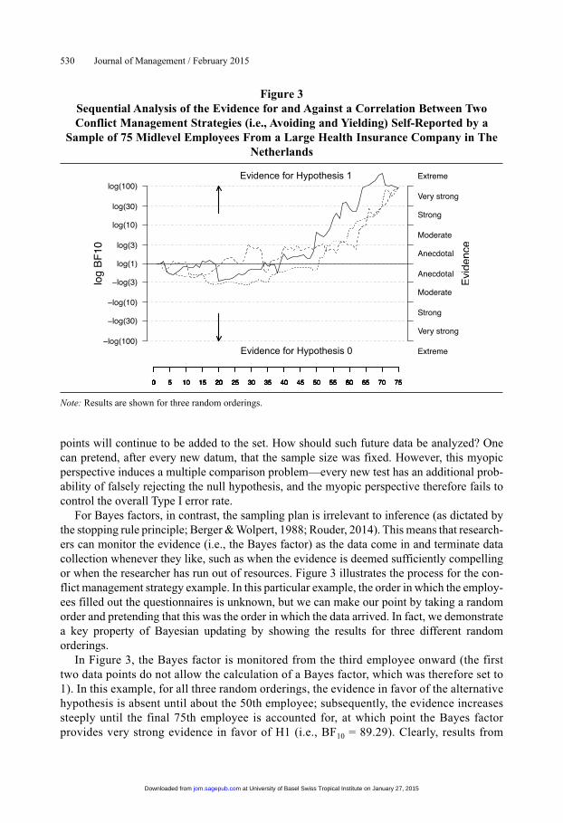
For Bayes factors, in contrast, the sampling plan is irrelevant to inference (as dictated by the stopping rule principle; Berger & Wolpert, 1988; Rouder, 2014). This means that research-ers can monitor the evidence (i.e., the Bayes factor) as the data come in and terminate data collection whenever they like, such as when the evidence is deemed sufficiently compelling or when the researcher has run out of resources. Figure 3 illustrates the process for the con-flict management strategy example. In this particular example, the order in which the employ-ees filled out the questionnaires is unknown, but we can make our point by taking a random order and pretending that this was the order in which the data arrived. In fact, we demonstrate a key property of Bayesian updating by showing the results for three different random orderings.

In Figure 3, the Bayes factor is monitored from the third employee onward (the first two data points do not allow the calculation of a Bayes factor, which was therefore set to 1). In this example, for all three random orderings, the evidence in favor of the alternative hypothesis is absent until about the 50th employee; subsequently, the evidence increases steeply until the final 75th employee is accounted for, at which point the Bayes factor provides very strong evidence in favor of H1 (i.e., BF10 = 89.29). Clearly, results from

Figure 3Sequential Analysis of the Evidence for and Against a Correlation Between Two Conflict Management Strategies (i.e., Avoiding and Yielding) Self-Reported by a

Sample of 75 Midlevel Employees From a Large Health Insurance Company in The Netherlands

Evidence for Hypothesis 1

Evidence for Hypothesis 0

Note: Results are shown for three random orderings.




new employees can be added and the evidence can be updated continually. Note that the final Bayes factor is equal for all three random orderings, illustrating the fact that for exchangeable data, Bayesian conclusions do not depend on the order in which the obser-vations arrived or indeed on whether the data became available simultaneously or one at a time.

Bayesian Hypothesis Testing for Regression Models

Across the empirical sciences, regression analysis is one of the most popular statistical tools: a dependent or criterion variable (e.g., income) is accounted for by a weighted combi-nation of independent or predictor variables (e.g., level of education, age, gender). In man-agement research, the inclusion of particular predictor variables often amounts to the test of a specific theory or hypothesis in the sense that statistical support for the inclusion of the predictor variables yields conceptual support for the theory that postulated the importance of those variables.

The Bayesian principles outlined in the previous section also hold for regression models (e.g., Liang et al., 2008; Rouder & Morey, 2012). Suppose model MX includes x predictors, and model MY includes x predictors plus one additional predictor. The evidence for the inclu-sion of this additional predictor is then given by BFYX = p(D | MY) / p(D | MX). Now suppose a third model, MZ, again includes one predictor more than MY. The evidence for MZ over MX is BFZX = p(D | MZ ) / p(D | MX). Thus, we know the strength of evidence for both MY and MZ versus the simplest model MX. Then it is easy to see that the evidence for MY versus MZ can be obtained by transitivity as follows: BFZY = BFZX / BFYX. Thus, all that is required to assess the evidence for and against the inclusion of predictors is the ability to compute the Bayes factor for any specific model against a common baseline model without predictors; the Bayes factors for different extended models against each other can then be obtained through transitivity.

The remaining difficulty is to specify suitable priors for the beta regression coefficients. Here we adopt an objective Bayesian perspective and specify priors based on general desid-erata instead of on substantive knowledge that is unique to a particular application. In linear regression models, the most popular objective prior specification scheme is inspired by the pioneering work of Harold Jeffreys and Arnold Zellner. This JZS prior specification scheme (Bayarri, Berger, Forte, & Garcia-Donato, 2012; Jeffreys, 1961; Liang et al., 2008; Rouder & Morey, 2012; Zellner & Siow, 1980) assigns a multivariate “fat-tail Normal” distribution to the regression coefficients.3

Detailed mathematical derivation, explanation, and motivation for the JZS prior is pro-vided elsewhere (i.e., Liang et al., 2008; Rouder & Morey, 2012; Wetzels, Grasman, & Wagenmakers, 2012). Here the emphasis is on the conceptual interpretation and practical utility of the Bayes factors associated with the JZS specification. In this context, it is impor-tant to emphasize that there exists user-friendly software to obtain the JZS Bayes factors—in particular, we attend the reader to Jeff Rouder’s Web-applet (http://pcl.missouri.edu/bf-reg) and the corresponding BayesFactor package in R. Appendix A includes the R code that we used for the analysis of the examples in this article, and Appendix B provides a step-by-step recipe on how to reproduce our results using Rouder’s Web-applet (see the online supple-mental material).


http://pcl.missouri.edu/bf-reg



An Example From the Journal of Management

The goal of this section is to underscore the advantages of JZS Bayes factor hypothesis testing for hierarchical regression when applied to a practical analysis problem in manage-ment research. Hierarchical regression4 is one of the most generic and popular methods of hypothesis testing used in the Journal of Management; a quick literature survey of all Journal of Management articles that were either “in press” or published in 2013 revealed that at least 11 articles used hierarchical regression.

In a hierarchical regression analysis, predictor variables are added to the regression equation sequentially, either one by one or in batches. The sequence by which the predic-tors are entered is determined by their hierarchy, which is motivated by theoretical con-siderations and the structure of the data. Usually, the batch of predictors added in the first step represents nuisance variables that are outside the immediate focus of interest. Such variables may include demographic information, such as socioeconomic status, gender, and age. In the next step, the researcher adds a variable of interest (e.g., communication style) and judges the extent to which this variable adds anything over and above the nui-sance variables that were added in the first step. At every next step, new predictors can be added to the regression equation, and the order of inclusion usually reflects an increasing level of sophistication of the hypotheses under consideration. For instance, the third step may feature a predictor that quantifies the interaction between communication style and prosocial role expectations. At any step, the statistical support for the hypothesis that postulates the presence of the new predictors is determined by the increase in variance explained, as formalized by an F test (Cohen & Cohen, 1983) that follows the logic of pNHST.

Below, we outline two different ways in which Bayes factors allow researchers to assess the importance of predictors: covariate testing and model comparison (Rouder & Morey, 2012). For concreteness, our points are illustrated using a design from Dierdorff et al. (2012). As we did not have access to the original data, we chose to make our points using simulated data generated to yield summary statistics as similar as possible to those that were reported for the original data. These simulated data form the basis of our analy-sis; the file with simulated data can be found online5 so that the interested reader can confirm and redo our analysis. Because the data are simulated, no substantive conclusions can be attached to the results with respect to the original data by Dierdorff et al. Instead, our aim is to illustrate the JZS Bayes factor procedure using an example of realistic complexity.

Theoretical Background of the Dierdorff et al. (2012) Study

The study of Dierdorff et al. focused on citizenship, a concept defined as the set of “coop-erative, helpful behaviors extending beyond job requirements” (2012: 573). Citizenship is affected both by work context and by role expectations, that is, the “beliefs about what is required for successful role performance” (575).

On the basis of an extensive literature review and detailed reasoning process, Dierdorff et al. proposed the following five hypotheses about the effects of work context and role expectations on citizenship:




“Hypothesis 1: Prosocial role expectations are positively related to citizenship behavior.” (2012: 577)

“Hypothesis 2: The relationship between role expectations and citizenship is stronger in more inter-dependent contexts.” (579)

“Hypothesis 3: The relationship between role expectations and citizenship is stronger in more socially supportive contexts.” (580)

“Hypothesis 4: The relationship between role expectations and citizenship is stronger in more autonomous contexts.” (581)

“Hypothesis 5: The relationship between role expectations and citizenship is weaker in more ambig-uous contexts.” (581)

In the Dierdorff et al. study, these hypotheses were tested using data from two sources: (1) self-report surveys filled out by 198 full-time employees and (2) a performance evaluation form completed by the employee’s immediate supervisor.

Frequentist Analysis

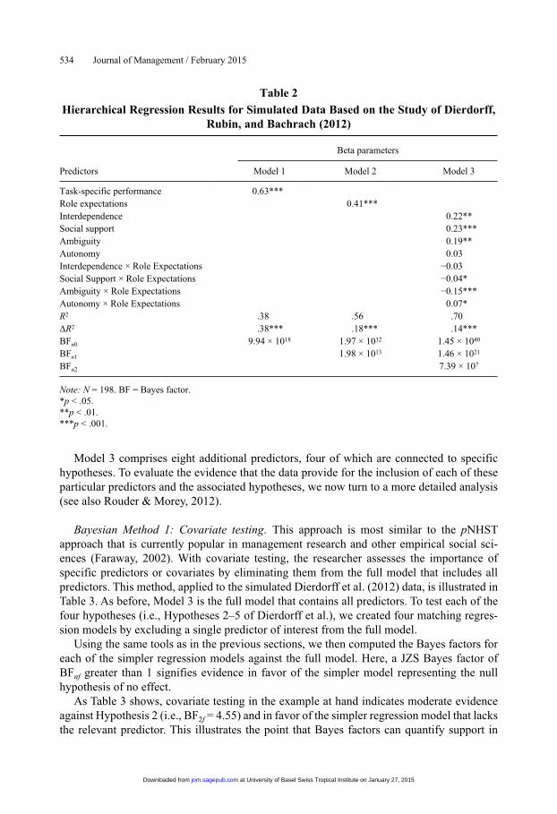
As mentioned above, we used the information reported in the Dierdorff et al. (2012) study to create a simulated data set that was as similar as possible to the original. All of the follow-ing analyses were conducted on the simulated data set. In this section, we discuss the fre-quentist analysis plan as followed by Dierdorff and colleagues. Table 2 summarizes the main findings (cf. Table 2 in Dierdorff et al.).

As is customary in hierarchical regression (Cohen & Cohen, 1983), the predictors of interest were added in steps. In the first step, the control variable “task-specific perfor-mance” was included as a predictor (i.e., Model 1), and this yields an R2 of .38. In the second step, the variable “role expectations” was added (i.e., Model 2), allowing a test of Hypothesis 1. As expected, Hypothesis 1 was confirmed: Inclusion of “role expectation” increases R2 from .38 to .56; in addition, the beta coefficient equals .41 (p < .001). In the third step, all remaining variables were added simultaneously (i.e., Model 3). The assess-ment of Hypotheses 2 through 5 then proceeds by inference on the beta coefficients for the specific predictors from Model 3.

In particular, frequentist inference suggests that the data do not support Hypothesis 2 (β = −0.03, p > .05), but they do support Hypotheses 3, 4, and 5 (β = −0.04, p < .05; β = 0.07, p < .05; β = −0.15, p < .001, respectively).6

Bayesian Analysis

From R2, the number of predictors, and the sample size, one can compute the JZS Bayes factors for Models 1, 2, and 3 against the null model (see the appendices in the online supple-mental material for R code using the BayesFactor package and for information on Jeff Rouder’s Web-applet http://pcl.missouri.edu/bf-reg); as before, all other Bayes factors can then be obtained by transitivity. Consistent with the frequentist analysis, results showed that the JZS Bayes factors indicated decisive support for Model 3 over Model 2 (i.e., BF32 = 7.39 × 107), Model 2 over Model 1 (i.e., BF21 = 1.98 × 1013), and Model 1 over the null model (BF10 = 9.94 × 1018).





Model 3 comprises eight additional predictors, four of which are connected to specific hypotheses. To evaluate the evidence that the data provide for the inclusion of each of these particular predictors and the associated hypotheses, we now turn to a more detailed analysis (see also Rouder & Morey, 2012).

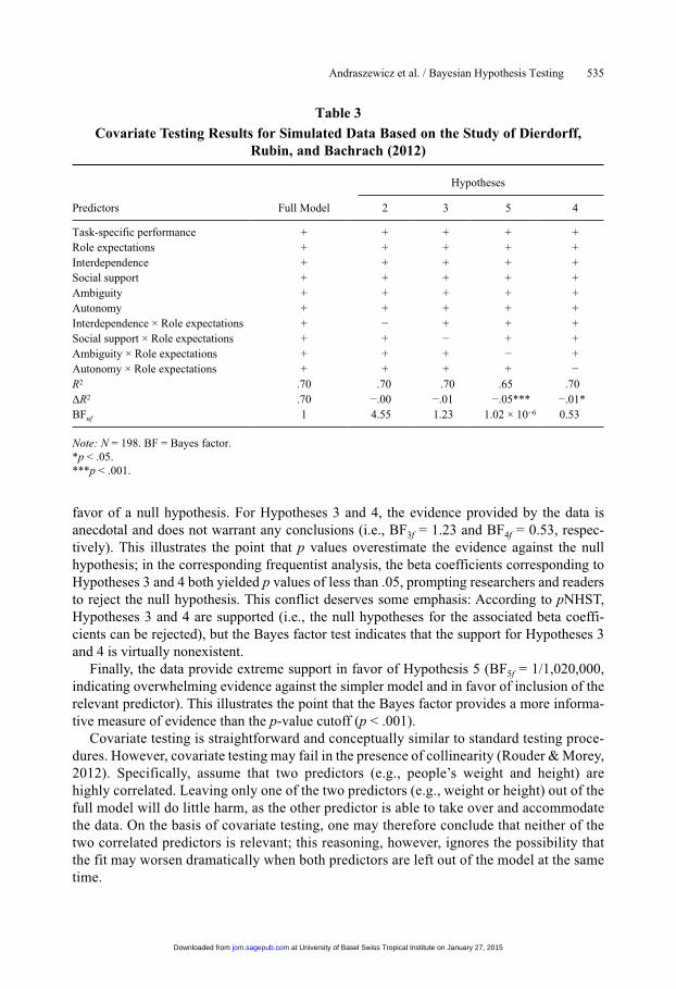
Bayesian Method 1: Covariate testing. This approach is most similar to the pNHST approach that is currently popular in management research and other empirical social sci-ences (Faraway, 2002). With covariate testing, the researcher assesses the importance of specific predictors or covariates by eliminating them from the full model that includes all predictors. This method, applied to the simulated Dierdorff et al. (2012) data, is illustrated in Table 3. As before, Model 3 is the full model that contains all predictors. To test each of the four hypotheses (i.e., Hypotheses 2–5 of Dierdorff et al.), we created four matching regres-sion models by excluding a single predictor of interest from the full model.

Using the same tools as in the previous sections, we then computed the Bayes factors for each of the simpler regression models against the full model. Here, a JZS Bayes factor of BFnf greater than 1 signifies evidence in favor of the simpler model representing the null hypothesis of no effect.

As Table 3 shows, covariate testing in the example at hand indicates moderate evidence against Hypothesis 2 (i.e., BF2f = 4.55) and in favor of the simpler regression model that lacks the relevant predictor. This illustrates the point that Bayes factors can quantify support in

Table 2

Hierarchical Regression Results for Simulated Data Based on the Study of Dierdorff, Rubin, and Bachrach (2012)

Βeta parameters

Predictors Model 1 Model 2 Model 3

Task-specific performance 0.63*** Role expectations 0.41*** Interdependence 0.22**Social support 0.23***Ambiguity 0.19**Autonomy 0.03Interdependence × Role Expectations −0.03Social Support × Role Expectations −0.04*Ambiguity × Role Expectations −0.15***Autonomy × Role Expectations 0.07*R2 .38 .56 .70ΔR2 .38*** .18*** .14***BFn0 9.94 × 1018 1.97 × 1032 1.45 × 1040

BFn1 1.98 × 1013 1.46 × 1021

BFn2 7.39 × 107

Note: N = 198. BF = Bayes factor.*p < .05.**p < .01.***p < .001.




favor of a null hypothesis. For Hypotheses 3 and 4, the evidence provided by the data is anecdotal and does not warrant any conclusions (i.e., BF3f = 1.23 and BF4f = 0.53, respec-tively). This illustrates the point that p values overestimate the evidence against the null hypothesis; in the corresponding frequentist analysis, the beta coefficients corresponding to Hypotheses 3 and 4 both yielded p values of less than .05, prompting researchers and readers to reject the null hypothesis. This conflict deserves some emphasis: According to pNHST, Hypotheses 3 and 4 are supported (i.e., the null hypotheses for the associated beta coeffi-cients can be rejected), but the Bayes factor test indicates that the support for Hypotheses 3 and 4 is virtually nonexistent.

Finally, the data provide extreme support in favor of Hypothesis 5 (BF5f = 1/1,020,000, indicating overwhelming evidence against the simpler model and in favor of inclusion of the relevant predictor). This illustrates the point that the Bayes factor provides a more informa-tive measure of evidence than the p-value cutoff (p < .001).

Covariate testing is straightforward and conceptually similar to standard testing proce-dures. However, covariate testing may fail in the presence of collinearity (Rouder & Morey, 2012). Specifically, assume that two predictors (e.g., people’s weight and height) are highly correlated. Leaving only one of the two predictors (e.g., weight or height) out of the full model will do little harm, as the other predictor is able to take over and accommodate the data. On the basis of covariate testing, one may therefore conclude that neither of the two correlated predictors is relevant; this reasoning, however, ignores the possibility that the fit may worsen dramatically when both predictors are left out of the model at the same time.

Table 3

Covariate Testing Results for Simulated Data Based on the Study of Dierdorff, Rubin, and Bachrach (2012)

Hypotheses

Predictors Full Model 2 3 5 4

Task-specific performance + + + + +Role expectations + + + + +Interdependence + + + + +Social support + + + + +Ambiguity + + + + +Autonomy + + + + +Interdependence × Role expectations + − + + +Social support × Role expectations + + − + +Ambiguity × Role expectations + + + − +Autonomy × Role expectations + + + + −R2 .70 .70 .70 .65 .70ΔR2 .70 −.00 −.01 −.05*** −.01*BFnf 1 4.55 1.23 1.02 × 10−6 0.53

Note: N = 198. BF = Bayes factor.*p < .05.***p < .001.




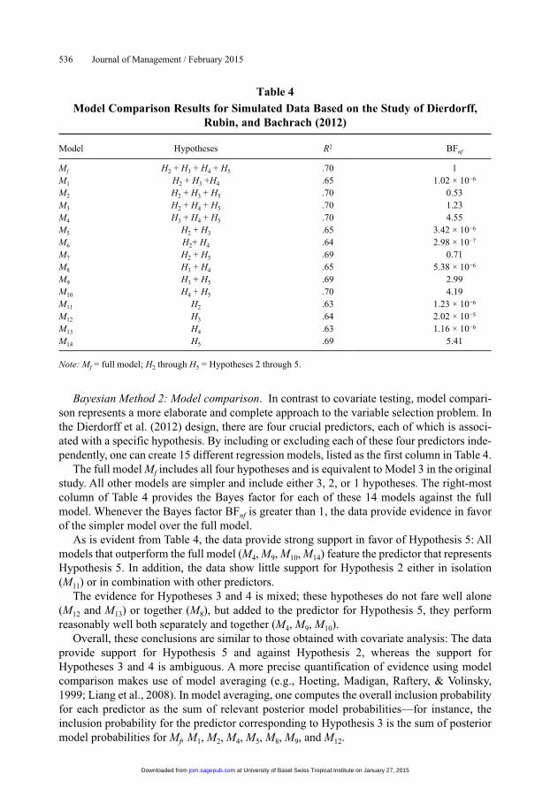
Bayesian Method 2: Model comparison. In contrast to covariate testing, model compari-son represents a more elaborate and complete approach to the variable selection problem. In the Dierdorff et al. (2012) design, there are four crucial predictors, each of which is associ-ated with a specific hypothesis. By including or excluding each of these four predictors inde-pendently, one can create 15 different regression models, listed as the first column in Table 4.

The full model Mf includes all four hypotheses and is equivalent to Model 3 in the original study. All other models are simpler and include either 3, 2, or 1 hypotheses. The right-most column of Table 4 provides the Bayes factor for each of these 14 models against the full model. Whenever the Bayes factor BFnf is greater than 1, the data provide evidence in favor of the simpler model over the full model.

As is evident from Table 4, the data provide strong support in favor of Hypothesis 5: All models that outperform the full model (M4, M9, M10, M14) feature the predictor that represents Hypothesis 5. In addition, the data show little support for Hypothesis 2 either in isolation (M11) or in combination with other predictors.

The evidence for Hypotheses 3 and 4 is mixed; these hypotheses do not fare well alone (M12 and M13) or together (M8), but added to the predictor for Hypothesis 5, they perform reasonably well both separately and together (M4, M9, M10).

Overall, these conclusions are similar to those obtained with covariate analysis: The data provide support for Hypothesis 5 and against Hypothesis 2, whereas the support for Hypotheses 3 and 4 is ambiguous. A more precise quantification of evidence using model comparison makes use of model averaging (e.g., Hoeting, Madigan, Raftery, & Volinsky, 1999; Liang et al., 2008). In model averaging, one computes the overall inclusion probability for each predictor as the sum of relevant posterior model probabilities—for instance, the inclusion probability for the predictor corresponding to Hypothesis 3 is the sum of posterior model probabilities for Mf, M1, M2, M4, M5, M8, M9, and M12.

Table 4

Model Comparison Results for Simulated Data Based on the Study of Dierdorff, Rubin, and Bachrach (2012)

Model Hypotheses R2 BFnf

Mf H2 + H3 + H4 + H5 .70 1M1 H2 + H3 +H4 .65 1.02 × 10−6

M2 H2 + H3 + H5 .70 0.53M3 H2 + H4 + H5 .70 1.23M4 H3 + H4 + H5 .70 4.55M5 H2 + H3 .65 3.42 × 10−6

M6 H2+ H4 .64 2.98 × 10−7

M7 H2 + H5 .69 0.71M8 H3 + H4 .65 5.38 × 10−6

M9 H3 + H5 .69 2.99M10 H4 + H5 .70 4.19M11 H2 .63 1.23 × 10−6

M12 H3 .64 2.02 × 10−5

M13 H4 .63 1.16 × 10−6

M14 H5 .69 5.41

Note: Mf = full model; H2 through H5 = Hypotheses 2 through 5.




General Discussion

Using Bayes factor hypothesis testing, researchers may monitor evidence as the data come in, they may quantify support in favor of the null hypothesis, and they may prevent themselves from prematurely rejecting the null hypothesis. The latter advantage is particu-larly acute in light of the recent crisis of confidence about the veracity of empirical find-ings (e.g., Pashler & Wagenmakers, 2012). It is entirely possible that the use of pNHST has exacerbated the replicability crisis (Johnson, 2013; Nuzzo, 2014; Wetzels, Matzke, Lee, Rouder, Iverson, & Wagenmakers, 2011) and that adoption of Bayes factor hypothesis test-ing may provide researchers with a more balanced and graded assessment of the evidence in favor of their hypotheses.7 This is underscored by comments from several statisticians; for instance, Dennis Lindley compared Bayes factors to Fisherian p values and concluded somewhat cynically:

There is therefore a serious and systematic difference between the Bayesian and Fisherian calculations, in the sense that a Fisherian approach much more easily casts doubt on the null value than does Bayes. Perhaps this is why significance tests are so popular with scientists: they make effects appear so easily. (1986a: 502)

A final comment comes from Berger and Delampady: “First and foremost, when testing precise hypotheses, formal use of P-values should be abandoned. Almost anything will give a better indication of the evidence provided by the data against H0” (1987: 330). For specific illustrations of this claim, we refer the reader to Edwards et al. (1963), Sellke et al. (2001), and Johnson (2013).

However, the conceptual advantages of Bayes factors may be offset by practical limita-tions and lingering concerns about feasibility and scope. In particular, one may wonder how to compute Bayes factors for other models that are popular in management research, one may wonder what Bayes factors tell us about the adequacy of a model considered in isolation, and finally, one may wonder whether the time is ripe for management researchers to become Bayesians. We deal with these issues in turn.

Bayes Factors for Other Models in Management Research

In the examples above, we have demonstrated the use of Bayes factors for the Pearson correlation coefficient and for hierarchical regression. However, the concept of Bayes factors is entirely general and carries over to many other models that are common in man-agement research. Although the literature has remained somewhat scattered, default Bayes factors have been developed for a number of relevant models, for instance, (1) contingency tables (e.g., Gunel & Dickey, 1974), (2) mixed analysis of variance designs (e.g., Rouder, Morey, Speckman, & Province, 2012), (3) mediation (Nuijten, Wetzels, Matzke, Dolan, & Wagenmakers, in press), (4) structural equation modeling (e.g., S.-Y. Lee, 2007; Song & Lee, 2012), and (5) generalized linear mixed models (Overstall & Forster, 2010).

A general approach that applies across a wide range of models is to use the Bayesian infor-mation criterion (BIC; Schwarz, 1978) as an approximation to a default Bayes factor. This approach has been promoted and explained by Adrian Raftery (1993, 1995; see also Masson, 2011; Wagenmakers, 2007). The main advantage of the BIC is its simplicity: For its




computation, it requires only the maximum likelihood, the number of free parameters, and the number of observations. The BIC approximation may fail in situations where sample size is low, where the relative complexity of a model is affected by the functional form of its param-eters (e.g., the difference between y = a + x and y = xa, where the free parameter a serves a very different function; see Myung & Pitt, 1997), and where the hierarchical nature of a model makes it difficult to determine the effective number of observations that the BIC should use (Pauler, 1998).

For the non-BIC versions of Bayes factors, several software packages are available, and we provide a selected overview here: Herbert Hoijtink, Joris Mulder, and colleagues have promoted their package BIEMS (e.g., Hoijtink, 2011; Mulder, Hoijtink, & de Leeuw, 2012); Zoltan Dienes has provided an online tutorial as well as software (http://www.lifesci.sussex.ac.uk/home/Zoltan_Dienes/inference/Bayes.htm); and, finally, Richard Morey has written the BayesFactor package for R (http://bayesfactorpcl.r-forge.r-project.org/), parts of which can be used through Jeff Rouder’s Web site (http://pcl.missouri.edu/bf-reg). We expect that in the near future, many Bayes factor hypothesis tests will be integrated into a single user-friendly package (e.g., JASP, http://jasp-stats.org/).

Bayes Factors Versus Absolute Goodness of Fit

The Bayes factor is inherently comparative: It assesses the support that the data provide for one model versus another. This is useful and informative, but it can also be misleading: Even though a specific model may outperform another in terms of the Bayes factor, both models may provide a poor account of the data, invalidating the inference. Thus, before drawing conclusions, it is important to assess absolute goodness of fit and confirm that the best model is also a good model.

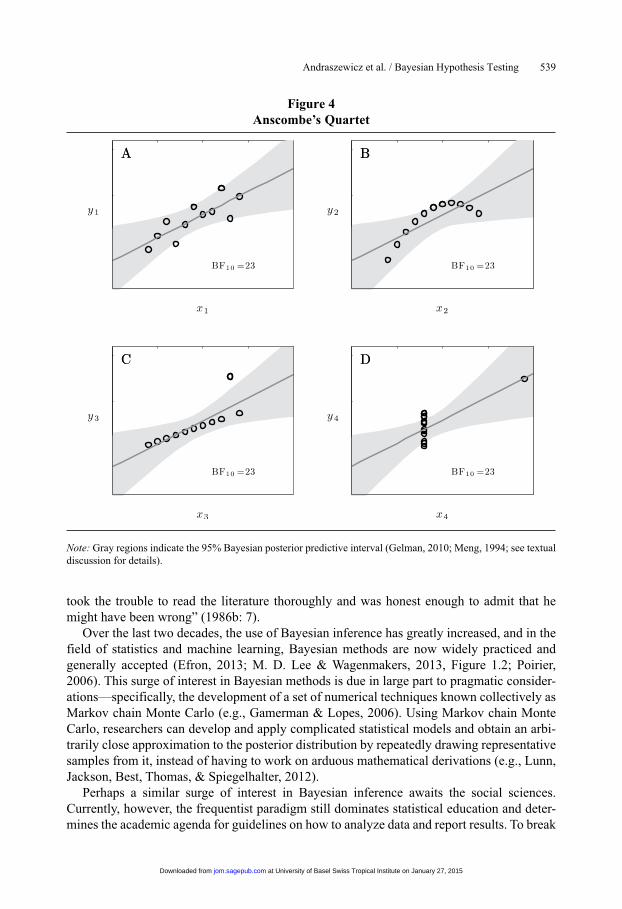
This important issue is highlighted in Anscombe’s quartet (Anscombe, 1973), shown here as Figure 4. Each panel shows a different data set, carefully constructed so that the variables have the same means, variances, and linear regression coefficient. For each data set, the Bayes factor is 23, indicating strong support for the presence of a linear association. A casual glance at the figure, however, convinces one that the statistical models and associated infer-ence are valid only for Figure 4A.

Model misfit can be assessed in several ways. Anscombe’s quartet suggests that inspect-ing data by eye can often be highly informative. In general, one can inspect structure in the residuals and assess the impact of individual data points by successively leaving them out of the analysis. Such methods for assessing absolute model fit can be carried out within both the frequentist and the Bayesian paradigm.

Should Management Researchers Become Bayesians?

Several general arguments have been mounted for and against Bayesian inference. Some researchers have tried to indicate explicitly why not every scientist is a Bayesian (e.g., Dennis, 1996; Efron, 1986). For instance, Dennis argued that, in contrast to Bayesian infer-ence, frequentist statistics has a “proven track record” (1996: 1101). Efron argued that “the high ground of scientific objectivity has been seized by the frequentists” (1986: 4). In response to Efron, Dennis Lindley stated that “every statistician would be a Bayesian if he


http://www.lifesci.sussex.ac.uk/home/Zoltan_Dienes/inference/Bayes.htm

http://www.lifesci.sussex.ac.uk/home/Zoltan_Dienes/inference/Bayes.htm

http://bayesfactorpcl.r-forge.r-project.org/


http://jasp-stats.org/



took the trouble to read the literature thoroughly and was honest enough to admit that he might have been wrong” (1986b: 7).

Over the last two decades, the use of Bayesian inference has greatly increased, and in the field of statistics and machine learning, Bayesian methods are now widely practiced and generally accepted (Efron, 2013; M. D. Lee & Wagenmakers, 2013, Figure 1.2; Poirier, 2006). This surge of interest in Bayesian methods is due in large part to pragmatic consider-ations—specifically, the development of a set of numerical techniques known collectively as Markov chain Monte Carlo (e.g., Gamerman & Lopes, 2006). Using Markov chain Monte Carlo, researchers can develop and apply complicated statistical models and obtain an arbi-trarily close approximation to the posterior distribution by repeatedly drawing representative samples from it, instead of having to work on arduous mathematical derivations (e.g., Lunn, Jackson, Best, Thomas, & Spiegelhalter, 2012).

Perhaps a similar surge of interest in Bayesian inference awaits the social sciences. Currently, however, the frequentist paradigm still dominates statistical education and deter-mines the academic agenda for guidelines on how to analyze data and report results. To break

Figure 4Anscombe’s Quartet

Note: Gray regions indicate the 95% Bayesian posterior predictive interval (Gelman, 2010; Meng, 1994; see textual discussion for details).




the frequentist stranglehold, the social sciences require more Bayesian course books (e.g., Dienes, 2008; Kruschke, 2010; M. D. Lee & Wagenmakers, 2013) and more user-friendly software packages that facilitate the application and interpretation of Bayesian methods (e.g., see Appendix B in the online supplemental material). In the end, we suspect that for the social sciences as for statistics and machine learning, the chances for widespread adoption of Bayesian methods depend primarily on practical considerations.

So should management scientists become Bayesians? Given the lack of user-friendly soft-ware and course material, a complete and wholesale shift does not appear to be practically feasible right now. However, it is possible for management scientists to apply Bayesian thinking and Bayesian procedures for an ever-growing subset of statistical models (e.g., cor-relation and hierarchical regression, as described above).

For these models, we believe it is productive and prudent to assess the Bayesian conclu-sions alongside the frequentist conclusions. It may happen, as we showed in the example on hierarchical regression, that a p value is lower than .05 but the Bayes factor indicates that the evidence is only anecdotal. At a minimum, such conflicts urge caution and suggest that the evidence is equivocal.

In conclusion, the JZS Bayes factor regression analysis is relatively easy to carry out. Researchers can construct their regression models and apply either the covariate testing or model comparison method described in the previous sections. Researchers familiar with the R programming language may benefit from downloading our analysis scripts and data, all of which is available online. Researchers who are more comfortable with Web interfaces may conduct JZS Bayes factor regression analysis through Jeff Rouder’s user-friendly Web-applet (see http://pcl.missouri.edu/bf-reg and Appendix B in the online supplemental material).

One may argue that in many situations, the data will pass the “interocular traumatic test” (i.e., when the pattern in the data is so evident that the conclusion hits you straight between the eyes; Edwards et al., 1963), and the results will be clear no matter what statistical para-digm is being used. Luckily, this is true; however, some data fail the interocular traumatic test and the results may indeed depend on the statistical paradigm that is used. In such cases, it seems worthwhile to not just base one’s statistical inference on frequentist methods alone but also rely on Bayesian techniques.

Notes1. Despite the conceptual divide between Bayesian credible intervals and frequentist confidence intervals, it

so happens that under uninformative priors, for a specific set of models and a specific set of parameters, there is numerical agreement between the credible interval and the confidence interval (Lindley, 1965).

2. As is becoming increasingly common, we use “hypothesis” and “model” interchangeably in this report. Models are used to encode or specify hypotheses, and hypothesis testing may be considered a form of model comparison.

3. The “fat-tail Normal” is a so-called Cauchy distribution (i.e., a t distribution with 1 degree of freedom). Compared to the Normal distribution, the Cauchy distribution has more mass in the tails.

4. Note the distinction to the kind of hierarchical regression that assumes a multilevel structure (e.g., Gelman & Hill, 2007).

5. The link to the simulated data is http://tinyurl.com/onlineSupplement.6. In what follows, we deliberately ignore the complication that, for the simulated data set, the beta coefficient

corresponding to Hypothesis 3 (Social Support × Role Expectations) does not have the correct sign—in the original data, the beta coefficient was estimated to be 0.11 instead of −0.04. This qualitative mismatch reveals that, despite considerable effort, we were unable to generate simulated data that matched the original data exactly.



http://tinyurl.com/onlineSupplement



7. Bayes factors are not a silver bullet; specifically, they are not robust to many questionable research practices, such as selective publication and selective reporting (Simmons, Nelson, & Simmonsohn, 2011). This underscores that any reasonable method for inference will be sensitive to the data it confronts according to the adage “garbage in, garbage out.”

ReferencesAitkin, M. 1991. Posterior Bayes factors. Journal of the Royal Statistical Society: Series B, 53: 111-142.Anscombe, F. J. 1973. Graphs in statistical analysis. The American Statistician, 27: 17-21.Bayarri, M. J., Berger, J. O., Forte, A., & Garcia-Donato, G. 2012. Criteria for Bayesian model choice with applica-

tion to variable selection. Annals of Statistics, 40: 1550-1577.Bechtoldt, M. N., de Dreu, C. K. W., Nijstad, B. A., & Zapf, D. 2010. Self-concept clarity and the management of

social conflict. Journal of Personality, 78: 539-574.Berger, J. O. 2006. Bayes factors. In S. Kotz, N. Balakrishnan, C. Read, B. Vidakovic, & N. L. Johnson (Eds.),

Encyclopedia of statistical sciences (2nd ed.), vol. 1: 378-386. Hoboken, NJ: Wiley.Berger, J. O., & Delampady, M. 1987. Testing precise hypotheses. Statistical Science, 2: 317-352.Berger, J. O., & Wolpert, R. L. 1988. The likelihood principle (2nd ed.). Hayward, CA: Institute of Mathematical

Statistics.Chiu, S.-C., & Sharfman, M. 2011. Legitimacy, visibility, and the antecedents of corporate social performance: An

investigation of the instrumental perspective. Journal of Management, 37: 1558-1585.Cohen, J. 1994. The earth is round (p < .05). American Psychologist, 49: 997-1003.Cohen, J., & Cohen, P. 1983. Applied multiple regression/correlation analysis for the behavioral sciences (2nd ed.).

Hillsdale, NJ: Erlbaum.Cox, D. R. 1958. Some problems connected with statistical inference. The Annals of Mathematical Statistics, 29:

357-372.Cumming, G. 2014. The new statistics: Why and how. Psychological Science, 25: 7-29.de Dreu, C. K. W., Evers, A., Beersma, B., Kluwer, E. S., & Nauta, A. 2001. A theory-based measure of conflict

management strategies in the workplace. Journal of Organizational Behavior, 22: 645-668.De Groot, A. D. 2014. The meaning of “significance” for different types of research [translated and annotated

by Eric-Jan Wagenmakers, Denny Borsboom, Josine Verhagen, Rogier Kievit, Marjan Bakker, Angelique Cramer, Dora Matzke, Don Mellenbergh, and Han L. J. van der Maas]. Acta Psychologica, 148: 188-194. (Original work published 1956)

Dennis, B. 1996. Discussion: Should ecologists become Bayesians? Ecological Applications, 6: 1095-1103.Dickey, J. M., & Lientz, B. P. 1970. The weighted likelihood ratio, sharp hypotheses about chances, the order of a

Markov chain. The Annals of Mathematical Statistics, 41: 214-226.Dienes, Z. 2008. Understanding psychology as a science: An introduction to scientific and statistical inference. New

York: Palgrave Macmillan.Dierdorff, E. C., Rubin, R. S., & Bachrach, D. G. 2012. Role expectations as antecedents of citizenship and the

moderating effects of work context. Journal of Management, 38: 573-598.Edwards, W., Lindman, H., & Savage, L. J. 1963. Bayesian statistical inference for psychological research.

Psychological Review, 70: 193-242.Efron, B. 1986. Why isn’t everyone a Bayesian? The American Statistician, 40: 1-5.Efron, B. 2013. A 250-year argument: Belief, behavior, and the bootstrap. Bulletin of the American Mathematical

Society, 50: 129-146.Faraway, J. J. 2002. Practical regression and ANOVA using R. http://www.maths.bath.ac.uk/~jjf23/book. Accessed

November 28, 2012.Gallistel, C. R. 2009. The importance of proving the null. Psychological Review, 116: 439-453.Gamerman, D., & Lopes, H. F. 2006. Markov chain Monte Carlo: Stochastic simulation for Bayesian inference.

Boca Raton, FL: Chapman & Hall/CRC.Gelman, A. 2010. Bayesian statistics then and now. Statistical Science, 25: 162-165.Gelman, A., & Hill, J. 2007. Data analysis using regression and multilevel/hierarchical models. Cambridge,

England: Cambridge University Press.Gelman, A., & Rubin, D. B. 1995. Avoiding model selection in Bayesian social research. Sociological Methodology,

25: 165-173.Gunel, E., & Dickey, J. 1974. Bayes factors for independence in contingency tables. Biometrika, 61: 545-557.


http://www.maths.bath.ac.uk/~jjf23/book/



Hoekstra, R., Morey, R. D., Rouder, J. N., & Wagenmakers, E.-J. 2014. Robust misinterpretation of confidence intervals. Psychonomic Bulletin & Review, 21: 1157-1164. doi:10.3758/s13423-013-0572-3

Hoeting, J. A., Madigan, D., Raftery, A. E., & Volinsky, C. T. 1999. Bayesian model averaging: A tutorial. Statistical Science, 14: 382-417.

Hoijtink, H. 2011. Informative hypotheses: Theory and practice for behavioral and social scientists. New York: Chapman & Hall/CRC.

Jeffreys, H. 1961. Theory of probability (3rd ed.). New York: Oxford University Press.Jeffreys, H. 1973. Scientific inference (3rd ed.). Cambridge, England: Cambridge University Press.Johnson, V. E. 2013. Revised standards for statistical evidence. Proceedings of the National Academy of Sciences,

USA, 110: 19313-19317.Kass, R. E., & Raftery, A. E. 1995. Bayes factors. Journal of the American Statistical Association, 90: 773-795.Kruschke, J. K. 2010. Doing Bayesian data analysis: A tutorial introduction with R and BUGS. Burlington, MA:

Academic Press.Lee, M. D., & Wagenmakers, E.-J. 2013. Bayesian modeling for cognitive science: A practical course. Cambridge,

England: Cambridge University Press.Lee, S.-Y. 2007. Structural equation modelling: A Bayesian approach. Chichester, England: Wiley.Lewis, S. M., & Raftery, A. E. 1997. Estimating Bayes factors via posterior simulation with the Laplace-Metropolis

estimator. Journal of the American Statistical Association, 92: 648-655.Liang, F., Paulo, R., Molina, G., Clyde, M. A., & Berger, J. O. 2008. Mixtures of g priors for Bayesian variable

selection. Journal of the American Statistical Association, 103: 410-423.Lindley, D. V. 1965. Introduction to probability & statistics from a Bayesian viewpoint. Part 2. Inference.

Cambridge, England: Cambridge University Press.Lindley, D. V. 1986a. Comment on “Tests of significance in theory and practice” by D. J. Johnstone. Journal of the

Royal Statistical Society: Series D (The Statistician), 35: 502-504.Lindley, D. V. 1986b. Comment on “Why isn’t everyone a Bayesian?” by Bradley Efron. The American Statistician,

40: 6-7.Lindley, D. V. 1993. The analysis of experimental data: The appreciation of tea and wine. Teaching Statistics, 15:

22-25.Liu, C. C., & Aitkin, M. 2008. Bayes factors: Prior sensitivity and model generalizability. Journal of Mathematical

Psychology, 52: 362-375.Livingston, B. A. 2014. Bargaining behind the scenes: Spousal negotiation, labor, and work-family burnout. Journal

of Management, 40: 949-977.Lunn, D., Jackson, C., Best, N., Thomas, A., & Spiegelhalter, D. 2012. The BUGS book: A practical introduction to

Bayesian analysis. Boca Raton, FL: Chapman & Hall/CRC Press.Masson, M. E. J. 2011. A tutorial on a practical Bayesian alternative to null-hypothesis significance testing. Behavior

Research Methods, 43: 679-690.Meehl, P. E. 1978. Theoretical risks and tabular asterisks: Sir Karl, Sir Ronald, and the slow progress of soft psy-

chology. Journal of Consulting and Clinical Psychology, 46: 806-834.Meng, X.-L. 1994. Posterior predictive p-values. Annals of Statistics, 22: 1142-1160.Morey, R. D., & Rouder, J. N. 2011. Bayes factor approaches for testing interval null hypotheses. Psychological

Methods, 16: 406-419.Morey, R. D., Rouder, J. N., Verhagen, A. J., & Wagenmakers, E.-J. 2014. Why hypothesis tests are essen-

tial for psychological science: A comment on Cumming. Psychological Science, 25: 1289-1290. doi:10.1177/0956797614525969

Mulder, J., Hoijtink, H., & de Leeuw, C. 2012. BIEMS: A Fortran 90 program for calculating Bayes factors for inequality and equality constrained models. Journal of Statistical Software, 46: 1-39.

Myung, I. J., Forster, M. R., & Browne, M. W. 2000. Guest editors’ introduction: Special issue on model selection. Journal of Mathematical Psychology, 44: 1-2.

Myung, I. J., & Pitt, M. A. 1997. Applying Occam’s razor in modeling cognition: A Bayesian approach. Psychonomic Bulletin & Review, 4: 79-95.

Nuijten, M. B., Wetzels, R., Matzke, D., Dolan, C. V., & Wagenmakers, E.-J. in press. A default Bayesian hypoth-esis test for mediation. Behavior Research Methods. doi:10.3758/s13428-014-0470-2

Nuzzo, R. 2014. Statistical errors. Nature, 506: 150-152.




Overstall, A. M., & Forster, J. J. 2010. Default Bayesian model determination methods for generalised linear mixed models. Computational Statistics & Data Analysis, 54: 3269-3288.

Pashler, H., & Wagenmakers, E.-J. 2012. Editors’ introduction to the special section on replicability in psychologi-cal science: A crisis of confidence? Perspectives on Psychological Science, 7: 528-530.

Pauler, D. K. 1998. The Schwarz criterion and related methods for normal linear models. Biometrika, 85: 13-27.Poirier, D. J. 2006. The growth of Bayesian methods in statistics and economics since 1970. Bayesian Analysis, 1:

969-980.Raftery, A. E. 1993. Bayesian model selection in structural equation models. In K. A. Bollen & J. S. Long (Eds.),

Testing structural equation models: 163-180. Newbury Park, CA: Sage.Raftery, A. E. 1995. Bayesian model selection in social research. Sociological Methodology, 25: 111-196.Rouder, J. N. 2014. Optional stopping: No problem for Bayesians. Psychonomic Bulletin & Review, 21: 301-308.Rouder, J. N., & Morey, R. D. 2012. Default Bayes factors for model selection in regression. Multivariate Behavioral

Research, 47: 877-903.Rouder, J. N., Morey, R. D., Speckman, P. L., & Province, J. M. 2012. Default Bayes factors for ANOVA designs.

Journal of Mathematical Psychology, 56: 356-374.Rouder, J. N., Speckman, P. L., Sun, D., Morey, R. D., & Iverson, G. 2009. Bayesian t tests for accepting and reject-

ing the null hypothesis. Psychonomic Bulletin & Review, 16: 225-237.Schervish, M. J. 1996. P values: What they are and what they are not. The American Statistician, 50: 203-206.Schwarz, G. 1978. Estimating the dimension of a model. Annals of Statistics, 6: 461-464.Sellke, T., Bayarri, M. J., & Berger, J. O. 2001. Calibration of p values for testing precise null hypotheses. The

American Statistician, 55: 62-71.Simmons, J. P., Nelson, L. D., & Simmonsohn, U. 2011. False-positive psychology: Undisclosed flexibility in data

collection and analysis allows presenting anything as significant. Psychological Science, 22: 1-8.Song, X.-Y., & Lee, S.-Y. 2012. A tutorial on the Bayesian approach for analyzing structural equation models.

Journal of Mathematical Psychology, 56: 135-148.Takkouche, B., Regueira-Mendez, C., Garcia-Closas, R., Figueiras, A., Gestal-Otero, J. J., & Hernan, M. A. 2002.

Intake of wine, beer, and spirits and the risk of clinical common cold. American Journal of Epidemiology, 155: 853-858.

Vanpaemel, W. 2010. Prior sensitivity in theory testing: An apologia for the Bayes factor. Journal of Mathematical Psychology, 54: 491-498.

Wagenmakers, E.-J. 2007. A practical solution to the pervasive problems of p values. Psychonomic Bulletin & Review, 14: 779-804.

Wagenmakers, E.-J., Lodewyckx, T., Kuriyal, H., & Grasman, R. 2010. Bayesian hypothesis testing for psycholo-gists: A tutorial on the Savage-Dickey method. Cognitive Psychology, 60: 158-189.

Wagenmakers, E.-J., & Waldorp, L. 2006. Model selection: Theoretical developments and applications [Special Issue]. Journal of Mathematical Psychology, 50(2): 99-214.

Wetzels, R., Grasman, R. P. P. P., & Wagenmakers, E.-J. 2012. A default Bayesian hypothesis test for ANOVA designs. The American Statistician, 66: 104-111.

Wetzels, R., Matzke, D., Lee, M. D., Rouder, J. N., Iverson, G. J., & Wagenmakers, E.-J. 2011. Statistical evi-dence in experimental psychology: An empirical comparison using 855 t tests. Perspectives on Psychological Science, 6: 291-298.

Wetzels, R., van Ravenzwaaij, D., & Wagenmakers, E.-J. in press. Bayesian analysis. In R. Cautin & S. Lilienfeld (Eds.), The encyclopedia of clinical psychology. Hoboken, NJ: Wiley-Blackwell.

Zellner, A., & Siow, A. 1980. Posterior odds ratios for selected regression hypotheses. In J. M. Bernardo, M. H. De Groot, D. V. Lindley, & A. F. M Smith (Eds.), Bayesian statistics: 558-603. Valencia, Spain: University Press.

Zyphur, M. J., & Oswald, F. L. 2015. Bayesian estimation and inference: A user’s guide. Journal of Management, 41: 390-420. doi:10.1177/0149206313501200



Documents

An Introduction to Bayesian Hypothesis Testing for ...scheibehenne.de/AndraszewiczScheibehenneEtAl.2015.pdf · Andraszewicz et al. / Bayesian Hypothesis Testing 523 Bayesian Inference