NBER WORKING PAPER SERIES

AN INTERTEMPORAL CAPM WITH STOCHASTIC VOLATILITY

John Y. CampbellStefano Giglio

Christopher PolkRobert Turley

Working Paper 18411http://www.nber.org/papers/w18411

NATIONAL BUREAU OF ECONOMIC RESEARCH1050 Massachusetts Avenue

Cambridge, MA 02138September 2012

We are grateful to Torben Andersen, Gurdip Bakshi, John Cochrane, Bjorn Eraker, Bryan Kelly, IanMartin, Sydney Ludvigson, Monika Piazzesi, Tuomo Vuolteenaho, and seminar participants at the2012 EFA, 2011 HBS Finance Unit research retreat, IESE, INSEAD, 2012 Spring NBER Asset PricingMeeting, NYU Stern, Oxford University, University of Paris Dauphine, University of Chicago, Universityof Edinburgh, and the 2012 WFA for comments. We thank Josh Coval, Ken French, Mila GetmanskySherman, and Tyler Shumway for providing data used in the analysis. The views expressed hereinare those of the authors and do not necessarily reflect the views of the National Bureau of EconomicResearch.

At least one co-author has disclosed a financial relationship of potential relevance for this research.Further information is available online at http://www.nber.org/papers/w18411.ack

NBER working papers are circulated for discussion and comment purposes. They have not been peer-reviewed or been subject to the review by the NBER Board of Directors that accompanies officialNBER publications.

© 2012 by John Y. Campbell, Stefano Giglio, Christopher Polk, and Robert Turley. All rights reserved.Short sections of text, not to exceed two paragraphs, may be quoted without explicit permission providedthat full credit, including © notice, is given to the source.

An Intertemporal CAPM with Stochastic VolatilityJohn Y. Campbell, Stefano Giglio, Christopher Polk, and Robert TurleyNBER Working Paper No. 18411September 2012JEL No. G12,N22

ABSTRACT

This paper extends the approximate closed-form intertemporal capital asset pricing model of Campbell(1993) to allow for stochastic volatility. The return on the aggregate stock market is modeled as oneelement of a vector autoregressive (VAR) system, and the volatility of all shocks to the VAR is anotherelement of the system. Our estimates of this VAR reveal novel low-frequency movements in marketvolatility tied to the default spread. We show that growth stocks underperform value stocks becausethey hedge two types of deterioration in investment opportunities: declining expected stock returns,and increasing volatility. Volatility hedging is also relevant for pricing risk-sorted portfolios and non-equityassets such as equity index options and corporate bonds.

John Y. CampbellMorton L. and Carole S.Olshan Professor of EconomicsDepartment of EconomicsHarvard UniversityLittauer Center 213Cambridge, MA 02138and NBERjohn_campbell@harvard.edu

Stefano GiglioUniversity of ChicagoBooth School of Business5807 S. Woodlawn AvenueChicago, IL 60637and NBERstefano.giglio@chicagobooth.edu

Christopher PolkDepartment of FinanceLondon School of EconomicsHoughton St.London WC2A 2AEUKc.polk@lse.ac.uk

Robert TurleyHarvard UniversityBaker Library 220DBoston MA 02163turley@fas.harvard.edu

An online appendix is available at:http://www.nber.org/data-appendix/w18411

1 Introduction

The fundamental insight of intertemporal asset pricing theory is that long-term investors

should care just as much about the returns they earn on their invested wealth as about the

level of that wealth. In a simple model with a constant rate of return, for example, the

sustainable level of consumption is the return on wealth multiplied by the level of wealth,

and both terms in this product are equally important. In a more realistic model with

time-varying investment opportunities, conservative long-term investors will seek to hold

“intertemporal hedges”, assets that perform well when investment opportunities deterio-

rate. Such assets should deliver lower average returns in equilibrium if they are priced from

conservative long-term investors’ first-order conditions.

Since the seminal work of Merton (1973) on the intertemporal capital asset pricing model

(ICAPM), a large empirical literature has explored the relevance of intertemporal considera-

tions for the pricing of financial assets in general, and the cross-sectional pricing of stocks in

particular. One strand of this literature uses the approximate accounting identity of Camp-

bell and Shiller (1988a) and the assumption that a representative investor has Epstein-Zin

utility (Epstein and Zin 1989) to obtain approximate closed-form solutions for the ICAPM’s

risk prices (Campbell 1993). These solutions can be implemented empirically if they are

combined with vector autoregressive (VAR) estimates of asset return dynamics (Campbell

1996). Campbell and Vuolteenaho (2004), Campbell, Polk, and Vuolteenaho (2010), and

Campbell, Giglio, and Polk (2012) use this approach to argue that value stocks outperform

growth stocks on average because growth stocks do well when the expected return on the

aggregate stock market declines; in other words, growth stocks have low risk premia because

they are intertemporal hedges for long-term investors.

A weakness of the papers cited above is that they ignore time-variation in the volatility of

stock returns. In general, investment opportunities may deteriorate either because expected

stock returns decline or because the volatility of stock returns increases, and it is an empirical

question which of these two types of intertemporal risk have a greater effect on asset returns.

We address this weakness in this paper by extending the approximate closed-form ICAPM to

allow for stochastic volatility. The resulting model explains risk premia in the stock market

using three priced risk factors corresponding to three important attributes of aggregate

market returns: revisions in expected future cash flows, discount rates, and volatility. An

attractive characteristic of the model is that the prices of these three risk factors depend on

only one free parameter, the long-horizon investor’s coefficient of risk aversion.

Since the long-horizon investor in our model cares mostly about persistent changes in

the investment opportunity set, there must be predictable variation in long-run volatility for

volatility risk to matter. Empirically, we implement our methodology using a vector autore-

gression (VAR) including stock returns, realized variance, and other financial indicators that

may be relevant for predicting returns and risk. Our VAR reveals low-frequency movements

in market volatility tied to the default spread, the yield spread of low-rated over high-rated

1

bonds. While this effect has received little attention in the literature, we argue that it is

sensible: Investors in risky bonds perceive the long-run component of volatility and incor-

porate this information when they set credit spreads, as risky bonds are short the option to

default. Moreover, we show that GARCH-based methods that filter only the information in

past returns in order to disentangle the short-run and long-run volatility components miss

this important low-frequency component.

With our novel model of long-run volatility in hand, we find that growth stocks have low

average returns because they outperform not only when the expected stock return declines,

but also when stock market volatility increases. Thus growth stocks hedge two types of

deterioration in investment opportunities, not just one. In the period since 1963 that creates

the greatest empirical difficulties for the standard CAPM, we find that the three-beta model

explains over 69% of the cross-sectional variation in average returns of 25 portfolios sorted by

size and book-to-market ratios. The model is not rejected at the 5% level while the CAPM

is strongly rejected. The implied coefficient of relative risk aversion is an economically

reasonable 9.63, in contrast to the much larger estimate of 20.70, which we get when we

estimate a comparable version of the two-beta CAPM of Campbell and Vuolteenaho (2004)

using the same data.2 This success is due in large part to the inclusion of volatility betas in

the specification. In particular, the spread in volatility betas in the cross section generates

an annualized spread in average returns of 6.52% compared to a comparable spread of 3.90%

and 2.24% for cash-flow and discount-rate betas.

We confirm that our findings are robust by expanding the set of test portfolios in two

important dimensions. First, we show that our three-beta model not only describes the cross

section of size- and book-to-market-sorted portfolios but also can explain the average returns

on risk-sorted portfolios. We examine risk-sorted portfolios in response to the argument

of Daniel and Titman (1997, 2012) and Lewellen, Nagel, and Shanken (2010) that asset-

pricing tests using only portfolios sorted by characteristics known to be related to average

returns, such as size and value, can be misleading. As tests that include risk-sorted portfolios

are unable to reject our intertemporal CAPM with stochastic volatility, we verify that the

model’s success is not simply due to the low-dimensional factor structure of the 25 size- and

book-to-market-sorted portfolios. Specifically, we show that sorts on stocks’ pre-formation

sensitivity to volatility news generate economically and statistically significant spread in both

post-formation volatility beta and average returns in a manner consistent with our model.

Interestingly, in the post-1963 period, sorts on past CAPM beta generate little spread in

post-formation cash-flow betas, but significant spread in post-formation volatility betas.

Since, in the three-beta model, covariation with aggregate volatility news has a negative

premium, the three-beta model also explains why stocks with high past CAPM betas have

offered relatively little extra return in the post-1963 sample.

Second, we show that our three-beta model can help explain average returns on non-

equity portfolios that are exposed to aggregate volatility risk. These portfolios include the

2The risk aversion estimate reported in Campbell and Vuolteenaho’s (2004) paper is 28.75.

2

S&P 100 index straddle of Coval and Shumway (2001), which is explicitly designed to be

highly correlated with aggregate volatility risk, and the risky bond factor of Fama and French

(1993), which should be sensitive to changes in aggregate volatility since risky corporate debt

is short the option to default. Consistent with this intuition, we find that compared to the

volatility beta of a value-minus-growth bet, the risky bond factor’s volatility beta is of the

same order of magnitude while the straddle’s volatility beta is more than 3 times larger

in absolute magnitude. These volatility betas are of the right sign to explain the abnormal

CAPM returns of the option and bond portfolios. Approximately 38% of the average straddle

return can be attributed to its three ICAPM betas, based purely on model estimates from

the cross section of equity returns. Additionally, when we price the joint cross-section of

equity, bond, and straddle returns our intertemporal CAPM with stochastic volatility is not

rejected at the 5-percent level while the CAPM is strongly rejected.

The organization of our paper is as follows. Section 2 reviews related literature. Section

3 lays out the approximate closed-form ICAPM and shows how to extend it to incorporate

stochastic volatility. While our main focus is on asset pricing without the use of consump-

tion data, we do also derive the implications of our model for consumption growth. Section

4 presents data, econometrics, and VAR estimates of the dynamic process for stock returns

and realized volatility. This section documents the empirical success of our model in fore-

casting long-run volatility. Section 5 turns to cross-sectional asset pricing and estimates a

representative investor’s preference parameters to fit a cross-section of test assets, taking the

dynamics of stock returns as given. This section also presents a set of robustness exercises

in which we vary our basic VAR specification for the dynamics of aggregate returns and risk,

and explore the underlying components of volatility betas for the market portfolio and for

value stocks versus growth stocks. Section 6 concludes.

2 Literature Review

Our work is complementary to recent research on the “long-run risk model” of asset prices

(Bansal and Yaron 2004) which can be traced back to insights in Kandel and Stambaugh

(1991). Both the approximate closed-form ICAPM and the long-run risk model start with

the first-order conditions of an infinitely lived Epstein-Zin representative investor. As orig-

inally stated by Epstein and Zin (1989), these first-order conditions involve both aggregate

consumption growth and the return on the market portfolio of aggregate wealth. Campbell

(1993) pointed out that the intertemporal budget constraint could be used to substitute

out consumption growth, turning the model into a Merton-style ICAPM. Restoy and Weil

(1998, 2011) used the same logic to substitute out the market portfolio return, turning the

model into a generalized consumption CAPM in the style of Breeden (1979).

Kandel and Stambaugh (1991) were the first researchers to study the implications for

asset returns of time-varying first and second moments of consumption growth in a model

3

with a representative Epstein-Zin investor. Specifically, Kandel and Stambaugh (1991) as-

sumed a four-state Markov chain for the expected growth rate and conditional volatility

of consumption, and provided closed-form solutions for important asset-pricing moments.

In the spirit of Kandel and Stambaugh (1991), Bansal and Yaron (2004) added stochastic

volatility to the Restoy-Weil model, and subsequent research on the long-run risk model has

increasingly emphasized the importance of stochastic volatility for generating empirically

plausible implications from this model (Bansal, Kiku, and Yaron 2012, Beeler and Campbell

2012). In this paper we give the approximate closed-form ICAPM the same capability to

handle stochastic volatility that its cousin, the long-run risk model, already possesses.

One might ask whether there is any reason to work with an ICAPM rather than a

consumption-based model given that these models are derived from the same set of assump-

tions. The ICAPM developed in this paper has several advantages. First, it describes risks

as they appear to an investor who takes asset prices as given and chooses consumption to

satisfy his budget constraint. This is the way risks appear to individual agents in the econ-

omy, and it seems important for economists to understand risks in the same way that market

participants do rather than relying exclusively on a macroeconomic perspective. Second,

the ICAPM allows an empirical analysis based on financial proxies for the aggregate market

portfolio rather than on accurate measurement of aggregate consumption. While there are

certainly challenges to the accurate measurement of financial wealth, financial time series are

generally available on a more timely basis and over longer sample periods than consumption

series. Third, the ICAPM in this paper is flexible enough to allow multiple state variables

that can be estimated in a VAR system; it does not require low-dimensional calibration of the

sort used in the long-run risk literature. Finally, the stochastic volatility process used here

governs the volatility of all state variables, including itself. We show that this assumption

fits financial data reasonably well, and it guarantees that stochastic volatility would always

remain positive in a continuous-time version of the model, a property that does not hold in

most current implementations of the long-run risk model.3

The closest precursors to our work are unpublished papers by Chen (2003) and Sohn

(2010). Both papers explore the effects of stochastic volatility on asset prices in an ICAPM

setting but make strong assumptions about the covariance structure of various news terms

when deriving their pricing equations. Chen (2003) assumes constant covariances between

shocks to the market return (and powers of those shocks) and news about future expected

market return variance. Sohn (2010) makes two strong assumptions about asset returns and

consumption growth, specifically that all assets have zero covariance with news about future

consumption growth volatility and that the conditional contemporaneous correlation between

the market return and consumption growth is constant through time. Duffee (2005) presents

evidence against the latter assumption. It is in any case unattractive to make assumptions

about consumption growth in an ICAPM that does not require accurate measurement of

consumption.

3Eraker (2008) and Eraker and Shaliastovich (2008) are exceptions.

4

Chen estimates a VAR with a GARCH model to allow for time variation in the volatility

of return shocks, restricting market volatility to depend only on its past realizations and not

those of the other state variables. His empirical analysis has little success in explaining the

cross-section of stock returns. Sohn uses a similar but more sophisticated GARCH model

for market volatility and tests how well short-run and long-run risk components from the

GARCH estimation can explain the returns of various stock portfolios, comparing the results

to factors previously shown to be empirically successful. In contrast, our paper incorporates

the volatility process directly in the ICAPM, allowing heteroskedasticity to affect and to

be predicted by all state variables, and showing how the price of volatility risk is pinned

down by the time-series structure of the model along with the investor’s coefficient of risk

aversion.

A working paper by Bansal, Kiku, Shaliastovich and Yaron (2012), contemporaneous

with our own, explores the effects of stochastic volatility in the long-run risk model. Like us,

they find stochastic volatility to be an important feature in the time series of equity returns.

Their work puts greater emphasis on the implied consumption dynamics while we focus on

the cross-sectional pricing implications of exposure to volatility news. More fundamentally,

there are differences in the underlying models. They assume that the stochastic process

driving volatility is homoskedastic, and in their cross-sectional analysis they impose that

changes in the equity risk premium are driven only by the conditional variance of the stock

market. The different modeling assumptions account for our contrasting empirical results;

we show that volatility risk is very important in explaining the cross-section of stock returns

while they find it has little impact on cross-sectional differences in risk premia.

Stochastic volatility has, of course, been explored in other branches of the finance litera-

ture. For example, Chacko and Viceira (2005) and Liu (2007) show how stochastic volatility

affects the optimal portfolio choice of long-term investors. Chacko and Viceira assume an

AR(1) process for volatility and argue that movements in volatility are not persistent enough

to generate large intertemporal hedging demands. Campbell and Hentschel (1992), Calvet

and Fisher (2007), and Eraker and Wang (2011) argue that volatility shocks will lower ag-

gregate stock prices by increasing expected returns, if they do not affect cash flows. The

strength of this volatility feedback effect depends on the persistence of the volatility process.

Coval and Shumway (2001), Ang, Hodrick, Xing, and Zhang (2006), and Adrian and Rosen-

berg (2008) present evidence that shocks to market volatility are priced risk factors in the

cross-section of stock returns, but they do not develop any theory to explain the risk prices

for these factors.

There is also an enormous literature in financial econometrics on modeling and forecasting

time-varying volatility. Since Engle’s (1982) seminal paper on ARCH, much of the literature

has focused on variants of the univariate GARCH model (Bollerslev 1986), in which return

volatility is modeled as a function of past shocks to returns and of its own lags (see Poon

and Granger (2003) and Andersen et al. (2006) for recent surveys). More recently, realized

volatility from high-frequency data has been used to estimate stochastic volatility processes

(Barndorff-Nielsen and Shephard 2002, Andersen et al. 2003). The use of realized volatility

5

has improved the modeling and forecasting of volatility, including its long-run component;

however, this literature has primarily focused on the information content of high-frequency

intra-daily return data. This allows very precise measurement of volatility, but at the same

time, given data availability constraints, limits the potential to use long time series to learn

about long-run movements in volatility. In our paper, we measure realized volatility only

with daily data, but augment this information with other financial time series that reveal

information investors have about underlying volatility components.

Amuch smaller literature has, like us, looked directly at the information in other variables

concerning future volatility. In early work, Schwert (1989) links movements in stock market

volatility to various indicators of economic activity, particularly the price-earnings ratio and

the default spread, finding relatively weak results. Engle, Ghysels and Sohn (2009) study

the effect of inflation and industrial production growth on volatility, finding a significant link

between the two, especially at long horizons. Campbell and Taksler (2003) look at the cross-

sectional link between corporate bond yields and equity volatility, emphasizing that bond

yields respond to idiosyncratic firm-level volatility as well as aggregate volatility. Two recent

papers, Paye (2012) and Christiansen et al. (2012), look at larger sets of potential predictors

of volatility, that include the default spread and/or valuation ratios, to study which ones

have predictive power for quarterly realized variance. The former, in a standard regression

framework, finds that a few variables, that include the commercial paper to Treasury spread

and the default spread, contain useful information for predicting volatility. The latter uses

Bayesian Model Averaging to determine which variables are most important for predicting

quarterly volatility, and documents the importance of the default spread and valuation ratios

in forecasting short-run volatility.

3 An Intertemporal Model with Stochastic Volatility

3.1 Asset pricing with time varying risk

Preferences

We begin by assuming a representative agent with Epstein-Zin preferences. We write

the value function as

=h(1− )

1−

+ ¡E£1−+1

¤¢1i 1−

(1)

where is consumption and the preference parameters are the discount factor risk aversion

, and the elasticity of intertemporal substitution . For convenience, we define =

(1− )(1− 1).

6

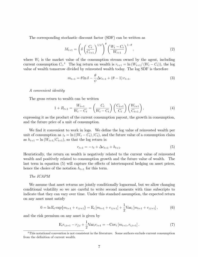
The corresponding stochastic discount factor (SDF) can be written as

+1 =

Ã

µ

+1

¶1! µ −

+1

¶1− (2)

where is the market value of the consumption stream owned by the agent, including

current consumption .4 The log return on wealth is +1 = ln (+1 ( − )), the log

value of wealth tomorrow divided by reinvested wealth today. The log SDF is therefore

+1 = ln −

∆+1 + ( − 1) +1 (3)

A convenient identity

The gross return to wealth can be written

1 ++1 =+1

−

=

µ

−

¶µ+1

¶µ+1

+1

¶ (4)

expressing it as the product of the current consumption payout, the growth in consumption,

and the future price of a unit of consumption.

We find it convenient to work in logs. We define the log value of reinvested wealth per

unit of consumption as = ln (( − ) ), and the future value of a consumption claim

as +1 = ln (+1+1), so that the log return is:

+1 = − +∆+1 + +1 (5)

Heuristically, the return on wealth is negatively related to the current value of reinvested

wealth and positively related to consumption growth and the future value of wealth. The

last term in equation (5) will capture the effects of intertemporal hedging on asset prices,

hence the choice of the notation +1 for this term.

The ICAPM

We assume that asset returns are jointly conditionally lognormal, but we allow changing

conditional volatility so we are careful to write second moments with time subscripts to

indicate that they can vary over time. Under this standard assumption, the expected return

on any asset must satisfy

0 = lnE exp{+1 + +1} = E [+1 + +1] +1

2Var [+1 + +1] (6)

and the risk premium on any asset is given by

E+1 − +1

2Var+1 = −Cov [+1 +1] (7)

4This notational convention is not consistent in the literature. Some authors exclude current consumption

from the definition of current wealth.

7

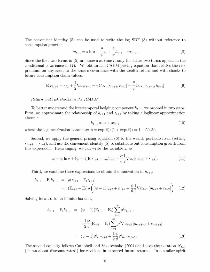
The convenient identity (5) can be used to write the log SDF (3) without reference to

consumption growth:

+1 = ln −

+

+1 − +1 (8)

Since the first two terms in (5) are known at time , only the latter two terms appear in the

conditional covariance in (7). We obtain an ICAPM pricing equation that relates the risk

premium on any asset to the asset’s covariance with the wealth return and with shocks to

future consumption claim values:

E+1 − +1

2Var+1 = Cov [+1 +1]−

Cov [+1 +1] (9)

Return and risk shocks in the ICAPM

To better understand the intertemporal hedging component +1, we proceed in two steps.

First, we approximate the relationship of +1 and +1 by taking a loglinear approximation

about ̄:

+1 ≈ + +1 (10)

where the loglinearization parameter = exp(̄)(1 + exp(̄)) ≈ 1− .

Second, we apply the general pricing equation (6) to the wealth portfolio itself (setting

+1 = +1), and use the convenient identity (5) to substitute out consumption growth from

this expression. Rearranging, we can write the variable as

= ln + ( − 1)E+1 +E+1 +

1

2Var [+1 + +1] (11)

Third, we combine these expressions to obtain the innovation in +1:

+1 − E+1 = (+1 − E+1)= (E+1 − E)

µ( − 1)+2 + +2 +

1

2Var+1 [+2 + +2]

¶ (12)

Solving forward to an infinite horizon,

+1 − E+1 = ( − 1)(E+1 − E)∞X=1

+1+

+1

2

(E+1 − E)

∞X=1

Var+ [+1+ + +1+]

= ( − 1)+1 +1

2

+1 (13)

The second equality follows Campbell and Vuolteenaho (2004) and uses the notation

(“news about discount rates”) for revisions in expected future returns. In a similar spirit

8

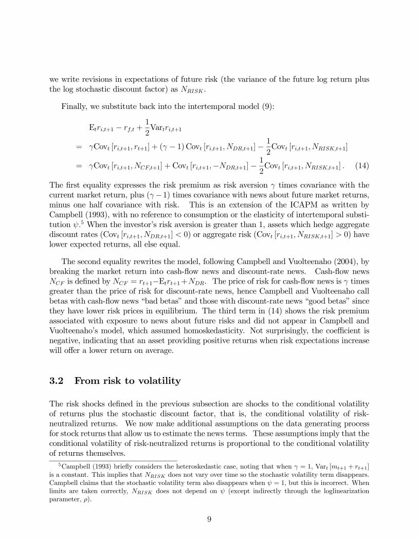
we write revisions in expectations of future risk (the variance of the future log return plus

the log stochastic discount factor) as .

Finally, we substitute back into the intertemporal model (9):

E+1 − +1

2Var+1

= Cov [+1 +1] + ( − 1)Cov [+1 +1]− 12Cov [+1 +1]

= Cov [+1 +1] +Cov [+1−+1]− 12Cov [+1 +1] (14)

The first equality expresses the risk premium as risk aversion times covariance with the

current market return, plus (−1) times covariance with news about future market returns,minus one half covariance with risk. This is an extension of the ICAPM as written by

Campbell (1993), with no reference to consumption or the elasticity of intertemporal substi-

tution 5 When the investor’s risk aversion is greater than 1, assets which hedge aggregate

discount rates (Cov [+1 +1] 0) or aggregate risk (Cov [+1 +1] 0) have

lower expected returns, all else equal.

The second equality rewrites the model, following Campbell and Vuolteenaho (2004), by

breaking the market return into cash-flow news and discount-rate news. Cash-flow news

is defined by = +1−E+1+. The price of risk for cash-flow news is times

greater than the price of risk for discount-rate news, hence Campbell and Vuolteenaho call

betas with cash-flow news “bad betas” and those with discount-rate news “good betas” since

they have lower risk prices in equilibrium. The third term in (14) shows the risk premium

associated with exposure to news about future risks and did not appear in Campbell and

Vuolteenaho’s model, which assumed homoskedasticity. Not surprisingly, the coefficient is

negative, indicating that an asset providing positive returns when risk expectations increase

will offer a lower return on average.

3.2 From risk to volatility

The risk shocks defined in the previous subsection are shocks to the conditional volatility

of returns plus the stochastic discount factor, that is, the conditional volatility of risk-

neutralized returns. We now make additional assumptions on the data generating process

for stock returns that allow us to estimate the news terms. These assumptions imply that the

conditional volatility of risk-neutralized returns is proportional to the conditional volatility

of returns themselves.

5Campbell (1993) briefly considers the heteroskedastic case, noting that when = 1, Var [+1 + +1]

is a constant. This implies that does not vary over time so the stochastic volatility term disappears.

Campbell claims that the stochastic volatility term also disappears when = 1, but this is incorrect. When

limits are taken correctly, does not depend on (except indirectly through the loglinearization

parameter, ).

9

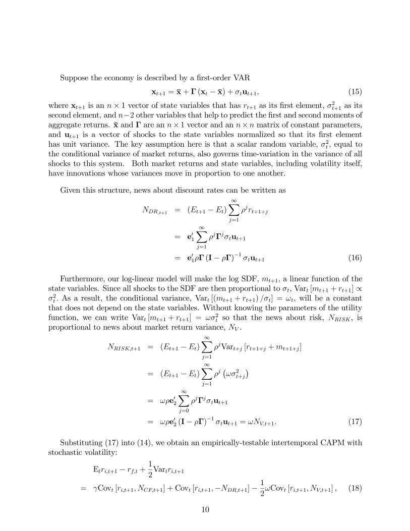
Suppose the economy is described by a first-order VAR

x+1 = x̄+ Γ (x − x̄) + u+1 (15)

where x+1 is an × 1 vector of state variables that has +1 as its first element, 2+1 as itssecond element, and −2 other variables that help to predict the first and second moments ofaggregate returns. x̄ and Γ are an × 1 vector and an × matrix of constant parameters,

and u+1 is a vector of shocks to the state variables normalized so that its first element

has unit variance. The key assumption here is that a scalar random variable, 2 , equal to

the conditional variance of market returns, also governs time-variation in the variance of all

shocks to this system. Both market returns and state variables, including volatility itself,

have innovations whose variances move in proportion to one another.

Given this structure, news about discount rates can be written as

+1= (+1 −)

∞X=1

+1+

= e01

∞X=1

Γu+1

= e01Γ (I− Γ)−1

u+1 (16)

Furthermore, our log-linear model will make the log SDF, +1 a linear function of the

state variables. Since all shocks to the SDF are then proportional to , Var [+1 + +1] ∝2 As a result, the conditional variance, Var [(+1 + +1) ] = , will be a constant

that does not depend on the state variables. Without knowing the parameters of the utility

function, we can write Var [+1 + +1] = 2 so that the news about risk, , is

proportional to news about market return variance, .

+1 = (+1 −)

∞X=1

Var+ [+1+ ++1+]

= (+1 −)

∞X=1

¡2+

¢= e02

∞X=0

Γu+1

= e02 (I− Γ)−1

u+1 = +1 (17)

Substituting (17) into (14), we obtain an empirically-testable intertemporal CAPM with

stochastic volatility:

E+1 − +1

2Var+1

= Cov [+1 +1] +Cov [+1−+1]− 12Cov [+1 +1] , (18)

10

where covariances with news about three key attributes of the market portfolio (cash flows,

discount rates, and volatility) describe the cross section of average returns.

The parameter is a nonlinear function of the coefficient of relative risk aversion , as

well as the VAR parameters and the loglinearization coefficient , but it does not depend on

the elasticity of intertemporal substitution except indirectly through the influence of on

. In the appendix, we show that solves:

2 = (1− )2Var£+1

¤+ (1− )Cov

£+1+1

¤+ 2

1

4Var

£+1

¤ (19)

We can see two main channels through which affects . First, a higher risk aversion–

given the underlying volatilities of all shocks–implies a more volatile stochastic discount

factor , and therefore a higher RISK. This effect is proportional to (1 − )2, so it in-

creases rapidly with . Second, there is a feedback effect on RISK through future risk:

appears on the right-hand side of the equation as well. Given that in our estimation we find

Cov£+1+1

¤ 0, this second effect makes increase even faster with .6

This equation can also be written directly in terms of the VAR parameters. If we define

and as the error-to-news vectors such that

1

+1 = +1 =

¡01 + 01Γ( − Γ)−1

¢+1 (20)

1

+1 = +1 =

¡02( − Γ)−1

¢+1 (21)

and define the covariance matrix of the residuals (scaled to eliminate stochastic volatility)

as Σ =Var[u+1], then solves

0 = 21

4Σ

0 − (1− (1− )Σ

0 ) + (1− )

2Σ

0 (22)

This quadratic equation for has two solutions. This result is an artifact of our linear

approximation of the Euler Equation, and the appendix shows that one of the solutions can

be disregarded. This false solution is easily identified by its implication that becomes

infinite as volatility shocks become small. The correct solution is

=1− (1− )Σ

0 −

p(1− (1− )Σ

0 )2 − (1− )2(Σ

0 )(Σ

0 )

12Σ

0

(23)

6Bansal, Kiku, Shaliastovich and Yaron (2012) derive a similar expression. The equivalent expression

for in their case reduces to (1 − )2 as they impose that the volatility process is homoskedastic and the

conditional equity premium is driven solely by the stochastic volatility.

11

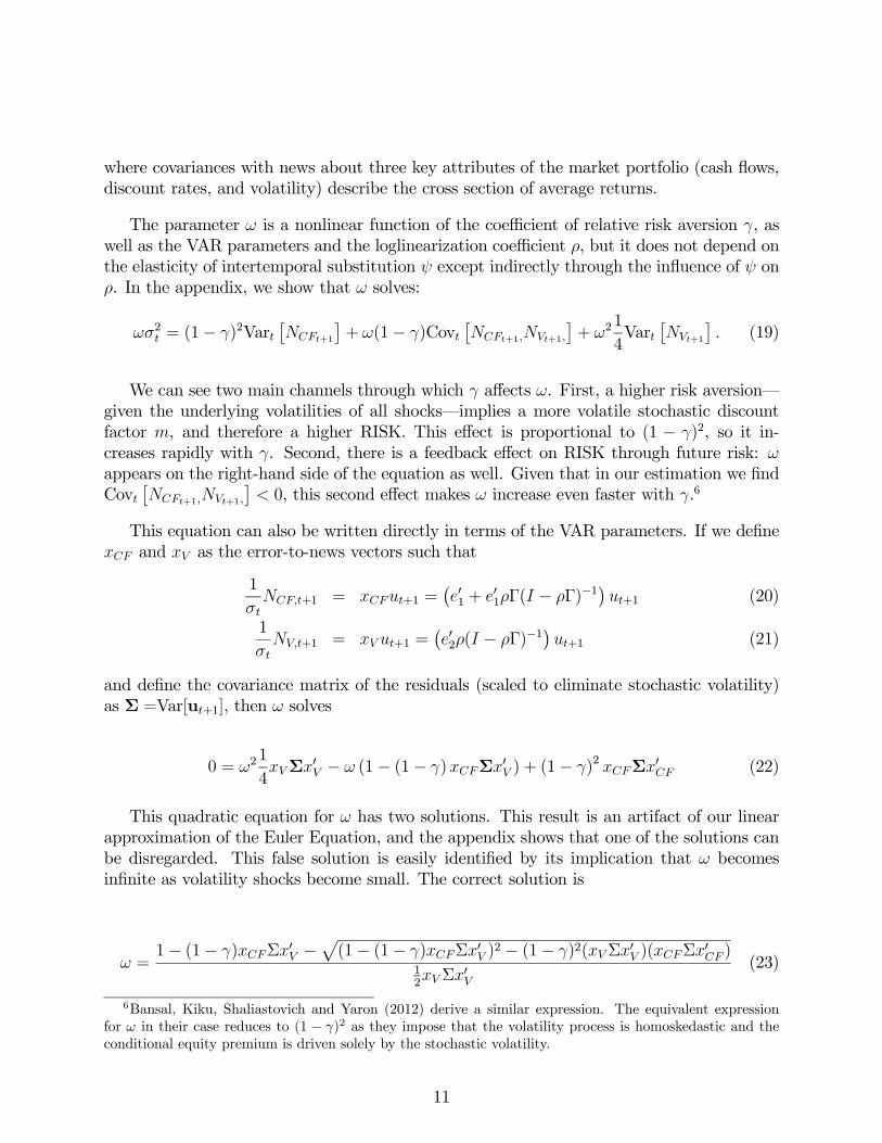
There is an additional disadvantage to the quadratic expression arising from our loglin-

earization. In the case where risk aversion, volatility shocks and cash flow shocks are large

enough, as measured by the product (1−)2(Σ0 )(Σ0 ). equation (22) may delivera complex rather than a real value for . While the conditional variance Var[+1 + +1]

from which we define will be both real and finite, the loglinear approximation may not

allow for a real solution in an economically important region of the parameter space. Given

our VAR estimates of the variance and covariance terms, we find equation (22) yields a real

solution as ranges from zero to 693.

To allow for larger values in our risk aversion parameter, we consider an alternative

approximation. If we linearize the right hand side of equation (19) around = 0 we can

approximate Var[+1 + +1] as a linear, rather than quadratic, function of . We then

have

≈ (1− )2(Σ0 )

1− (1− )(Σ0 )

(24)

which is now defined for all 0. Figure 1 plots as a function of using both the solution

in equation (23) and the approximation in (24) for values of up to 20.

By construction, they will yield similar solutions for values of close to one, where

gets close to 0 and volatility news becomes less and less important. In other words, it is

easy to show that our linearization preserves the property of the true model that as → 1,

→ 0 and

Var[+1 + +1]→ (1− )2Var[ ]

As risk aversion increases, we find that this approximate value for continues to resemble

the exact solution of the quadratic equation (22) in the region where a real solution exists.

We have also used numerical methods, similar to those proposed by Tauchen and Hussey

(1991), to solve the model and validate our estimates of for a range of values for that

include the region where the quadratic equation does not have a real solution.

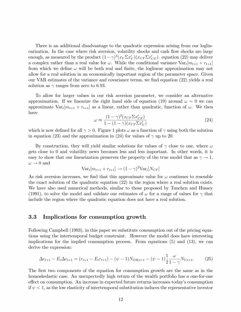
3.3 Implications for consumption growth

Following Campbell (1993), in this paper we substitute consumption out of the pricing equa-

tions using the intertemporal budget constraint. However the model does have interesting

implications for the implied consumption process. From equations (5) and (13), we can

derive the expression:

∆+1 −∆+1 = (+1 −+1)− ( − 1)+1 − ( − 1)12

1− +1 (25)

The first two components of the equation for consumption growth are the same as in the

homoskedastic case. An unexpectedly high return of the wealth portfolio has a one-for-one

effect on consumption. An increase in expected future returns increases today’s consumption

if 1, as the low elasticity of intertemporal substitution induces the representative investor

12

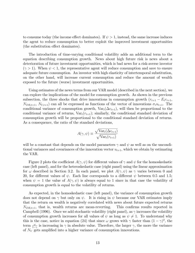
to consume today (the income effect dominates). If 1, instead, the same increase induces

the agent to reduce consumption to better exploit the improved investment opportunities

(the substitution effect dominates).

The introduction of time-varying conditional volatility adds an additional term to the

equation describing consumption growth. News about high future risk is news about a

deterioration of future investment opportunities, which is bad news for a risk-averse investor

( 1). When 1, the representative agent will reduce consumption and save to ensure

adequate future consumption. An investor with high elasticity of intertemporal substitution,

on the other hand, will increase current consumption and reduce the amount of wealth

exposed to the future (worse) investment opportunities.

Using estimates of the news terms from our VARmodel (described in the next section), we

can explore the implications of the model for consumption growth. As shown in the previous

subsection, the three shocks that drive innovations in consumption growth (+1 − +1,

+1, +1) can all be expressed as functions of the vector of innovations +1. The

conditional variance of consumption growth, Var(∆+1), will then be proportional to the

conditional variance of returns, Var(+1); similarly, the conditional standard deviation of

consumption growth will be proportional to the conditional standard deviation of returns.

As a consequence, the ratio of the standard deviations,

( ) ≡pVar(∆+1)pVar(+1)

will be a constant that depends on the model parameters and as well as on the uncondi-

tional variances and covariances of the innovation vector +1, which we obtain by estimating

the VAR.

Figure 2 plots the coefficient ( ) for different values of and for the homoskedastic

case (left panel), and for the heteroskedastic case (right panel) using the linear approximation

for described in Section 3.2. In each panel, we plot ( ) as varies between 0 and

20, for different values of . Each line corresponds to a different between 0.5 and 1.5;

when = 1 the value of ( ) is always equal to 1 since in that case the volatility of

consumption growth is equal to the volatility of returns.

As expected, in the homoskedastic case (left panel), the variance of consumption growth

does not depend on but only on . It is rising in because our VAR estimates imply

that the return on wealth is negatively correlated with news about future expected returns

+1 that is, wealth returns are mean-reverting. This confirms results reported in

Campbell (1996). Once we add stochastic volatility (right panel), as increases the volatility

of consumption growth increases for all values of as long as 6= 1. To understand whythis is the case, notice in equation (24) that since grows with faster than (1− )2, the

term 1− is increasing in in absolute value. Therefore, the larger , the more the variance

of gets amplified into a higher variance of consumption innovations.

13

Note also that for 1 and for high enough (i.e. in the bottom-right section of the

right panel), the volatility of consumption innovations is higher for lower values of . When

risk aversion is high, innovations in consumption are dominated by news about future risk.

Agents with very low or very high elasticity of intertemporal substitution, i.e. with far from

1, will tend to adjust their consumption strongly (in different directions) to volatility news.

Therefore, it is possible for individuals with lower elasticity of intertemporal substitution to

end up with amore volatile process for consumption innovations, due to their strong reaction

to volatility news.

4 Predicting Aggregate Stock Returns and Volatility

4.1 State variables

Our full VAR specification of the vector x+1 includes six state variables, five of which are

the same as in Campbell, Giglio and Polk (2011). To those five variables, we add an estimate

of conditional volatility. The data are all quarterly, from 1926:2 to 2011:4.

The first variable in the VAR is the log real return on the market, , the difference

between the log return on the Center for Research in Securities Prices (CRSP) value-weighted

stock index and the log return on the Consumer Price Index.

The second variable is expected market variance ( ). This variable is meant to

capture the volatility of market returns, , conditional on information available at time

, so that innovations to this variable can be mapped to the term described above.

To construct , we proceed as follows. We first construct a series of within-quarter

realized variance of daily returns for each time , . We then run a regression of

+1 on lagged realized variance ( ) as well as the other five state variables at

time . This regression then generates a series of predicted values for at each time

+ 1, that depend on information available at time : d +1. Finally, we define our

expected variance at time to be exactly this predicted value at + 1:

≡ d +1

Note that though we describe our methodology in a two-step fashion where we first estimate

and then use in a VAR, this is only for interpretability. Indeed, this approach

to modeling can be considered a simple renormalization of equivalent results we would

find from a VAR that included directly.7

7Since we weight observations based on in the first stage and then reweight observations using

in the second stage, our two-stage approach in practice is not exactly the same as a one-stage

approach. However, Panel B of Table 12 shows that results from a -weighted single-step estimation

are qualitatively very similar to those produced by our two-stage approach.

14

The third variable is the price-earnings ratio () from Shiller (2000), constructed as

the price of the S&P 500 index divided by a ten-year trailing moving average of aggregate

earnings of companies in the S&P 500 index. Following Graham and Dodd (1934), Campbell

and Shiller (1988b, 1998) advocate averaging earnings over several years to avoid temporary

spikes in the price-earnings ratio caused by cyclical declines in earnings. We avoid any

interpolation of earnings as well as lag the moving average by one quarter in order to ensure

that all components of the time- price-earnings ratio are contemporaneously observable by

time . The ratio is log transformed.

Fourth, the term yield spread ( ) is obtained from Global Financial Data. We compute

the series as the difference between the log yield on the 10-Year US Constant Maturity

Bond (IGUSA10D) and the log yield on the 3-Month US Treasury Bill (ITUSA3D).

Fifth, the small-stock value spread ( ) is constructed from data on the six “elementary”

equity portfolios also obtained from Professor French’s website. These elementary portfolios,

which are constructed at the end of each June, are the intersections of two portfolios formed

on size (market equity, ME) and three portfolios formed on the ratio of book equity to market

equity (BE/ME). The size breakpoint for year is the median NYSE market equity at the

end of June of year t. BE/ME for June of year is the book equity for the last fiscal year

end in − 1 divided by ME for December of − 1. The BE/ME breakpoints are the 30thand 70th NYSE percentiles.

At the end of June of year , we construct the small-stock value spread as the difference

between the ln() of the small high-book-to-market portfolio and the ln()

of the small low-book-to-market portfolio, where BE and ME are measured at the end of

December of year − 1. For months from July to May, the small-stock value spread is

constructed by adding the cumulative log return (from the previous June) on the small low-

book-to-market portfolio to, and subtracting the cumulative log return on the small high-

book-to-market portfolio from, the end-of-June small-stock value spread. The construction

of this series follows Campbell and Vuolteenaho (2004) closely.

The sixth variable in our VAR is the default spread ( ), defined as the difference

between the log yield on Moody’s BAA and AAA bonds. The series is obtained from the

Federal Reserve Bank of St. Louis. Campbell, Giglio and Polk (2011) add the default spread

to the Campbell and Vuolteenaho (2004) VAR specification in part because that variable is

known to track time-series variation in expected real returns on the market portfolio (Fama

and French, 1989), but mostly because shocks to the default spread should to some degree

reflect news about aggregate default probabilities. Of course, news about aggregate default

probabilities should in turn reflect news about the market’s future cash flows.

15

4.2 Short-run volatility estimation

In order for the regression model that generates to be consistent with a reasonable

data-generating process for market variance, we deviate from standard OLS in two ways.

First, we constrain the regression coefficients to produce fitted values (i.e. expected market

return variance) that are positive. Second, given that we explicitly consider heteroskedas-

ticity of the innovations to our variables, we estimate this regression using Weighted Least

Squares (WLS), where the weight of each observation pair ( +1, x) is initially based

on the time- value of ( )−1. However, to ensure that the ratio of weights across obser-vations is not extreme, we shrink these initial weights towards equal weights. In particular,

we set our shrinkage factor large enough so that the ratio of the largest observation weight

to the smallest observation weight is always less than or equal to five. Though admittedly

somewhat ad hoc, this bound is consistent with reasonable priors of the degree of variation

over time in expected market return variance. More importantly, we show later (in Table 12

Panel B) that our results are robust to variation in this bound. Both the constraint on the

regression’s fitted values and the constraint on WLS observation weights bind in the sample

we study.

The results of the first stage regression generating the state variable are reported

in Table 1 Panel A. Perhaps not surprisingly, past realized variance strongly predicts future

realized variance. More importantly, the regression documents that an increase in either

or predicts higher future realized volatility. Both of these results are very statistically

significant and are a novel finding of the paper. In particular, the fact that we find that very

persistent variables like PE and DEF forecast next period’s volatility indicates a potential

important role in volatility news for lower frequency or long-run movements in stochastic

volatility.

We argue that the links we find are sensible. Investors in risky bonds incorporate their

expectation of future volatility when they set credit spreads, as risky bonds are short the

option to default. Therefore we expect higher to be associated with higher .

The result that higher predicts higher might seem surprising at first, but one

has to remember that the coefficient indicates the effect of a change in holding constant

the other variables, in particular the default spread. Since the default spread should also

generally depend on the equity premium and since most of the variation in is due to

variation in the equity premium, for a given value of the default spread, a relatively high

value of implies a relatively higher level of future volatility. Thus cleans up the

information in concerning future volatility.

The 2 of this regression is just over 23%. The relatively low 2 masks the fact that

the fit is indeed quite good, as we can see from Figure 3, in which and are

plotted together. The 2 is heavily influenced by the occasional spikes in realized variance,

which the simple linear model we use is not able to capture. Indeed, our WLS approach

downweights the importance of those spikes in the estimation procedure.

16

The internet appendix to this paper (Campbell, Giglio, Polk, and Turley 2012) reports

descriptive statistics for these variables for the full sample, the early sample, and the modern

sample. Consistent with Campbell, Giglio and Polk (2012), we document high correlation

between and both and . The table also documents the persistence of both

and (autocorrelations of 0.524 and 0.740 respectively) and the high correlation

between these variance measures and the default spread.

Perhaps the most notable difference between the two subsamples is that the correlation

between and several of our other state variables changes dramatically. In the early

sample, is quite negatively correlated with both and . In the modern sample,

is essentially uncorrelated with and quite positively correlated with . As a

consequence, since is just a linear combination of our state variables, the correlation

between and changes sign across the two samples. In the early sample, this

correlation is very negative, with a value of -0.511. This strong negative correlation reflects

the high volatility that occurred during the Great Depression when prices were relatively

low. In the modern sample, the correlation is positive, 0.140. The positive correlation

simply reflects the economic fact that episodes with high volatility and high stock prices,

such as the technology boom of the late 1990s, were more prevalent in this subperiod than

episodes with high volatility and low stock prices, such as the recession of the early 1980s.

4.3 Estimation of the VAR and the news terms

Following Campbell (1993), we estimate a first-order VAR as in equation (15), where x+1is a 6× 1 vector of state variables ordered as follows:

x+1 = [+1 +1 +1 +1 +1 +1]

so that the real market return +1 is the first element and is the second element. x̄

is a 6×1 vector of the means of the variables, and Γ is a 6×6 matrix of constant parameters.Finally, u+1 is a 6×1 vector of innovations, with the conditional variance-covariance matrixof u+1 a constant:

Σ = Var(u+1)

so that the parameter 2 scales the entire variance-covariance matrix of the vector of inno-

vations.

The first-stage regression forecasting realized market return variance described in the

previous section generates the variable . The theory in Section 3 assumes that 2 ,

proxied for by , scales the variance-covariance matrix of state variable shocks. Thus,

as in the first stage, we estimate the second-stage VAR using WLS, where the weight of each

observation pair (x+1, x) is initially based on ( )−1. We continue to constrain both

the weights across observations and the fitted values of the regression forecasting .

17

Table 1 Panel B presents the results of the VAR estimation for the full sample (1926:2

to 2011:4). We report bootstrap standard errors for the parameter estimates of the VAR

that take into account the uncertainty generated by forecasting variance in the first stage.

Consistent with previous research, we find that negatively predict future returns, though

the t-statistic indicates only marginal significance. The value spread has a negative but not

statistically significant effect on future returns. In our specification, a higher conditional

variance, , is associated with higher future returns, though the effect is not statistically

significant. Of course, the relatively high degree of correlation among , , , and

complicates the interpretation of the individual effect of those variables. As for the

other novel aspects of the transition matrix, both high and high predict higher

future conditional variance of returns. High past market returns forecast lower ,

higher , and lower .8

Panel C of Table 1 reports the sample correlation and autocorrelation matrices of both

the unscaled residuals u+1 and the scaled residuals u+1. The correlation matrices report

standard deviations on the diagonals. There are a couple of aspects of these results to

note. For one thing, a comparison of the standard deviations of the unscaled and scaled

residuals provides a rough indication of the effectiveness of our empirical solution to the

heteroskedasticity of the VAR. In general, the standard deviations of the scaled residuals are

several times larger than their unscaled counterparts. More specifically, our approach implies

that the scaled return residuals should have unit standard deviation. Our implementation

results in a sample standard deviation of 0.562, that is relatively close to one.

Additionally, a comparison of the unscaled and scaled autocorrelation matrices reveals

that much of the sample autocorrelation in the unscaled residuals is eliminated by our WLS

approach. For example, the unscaled residuals in the regression forecasting the log real

return have an autocorrelation of -0.074. The corresponding autocorrelation of the scaled

return residuals is essentially zero, 0.002. Though the scaled residuals in the ,

and regression still display some negative autocorrelation, the unscaled residuals are

much more negatively autocorrelated.

Table 2 reports the coefficients of a regression of the squared unscaled residuals +1of each VAR equation on a constant and . These results are consistent with our

assumption that captures the conditional volatility of market returns (the coefficient

on in the regression forecasting the squared residuals of is 0.478). The fact that

significantly predicts with a positive sign all the squared errors of the VAR supports

our underlying assumption that one parameter (2 ) drives the volatility of all innovations.

8One worry is that many of the elements of the transition matrix are estimated imprecisely. Though these

estimates may be zero, their non-zero but statistically insignificant in-sample point estimates, in conjunction

with the highly-nonlinear function that generates discount-rate and volatility news, may result in misleading

estimates of risk prices. However, Table 12 Panel B shows that results are qualitatively similar if we instead

employ a partial VAR where, via a standard iterative process, only variables with -statistics greater than

1.0 are included in each VAR regression.

18

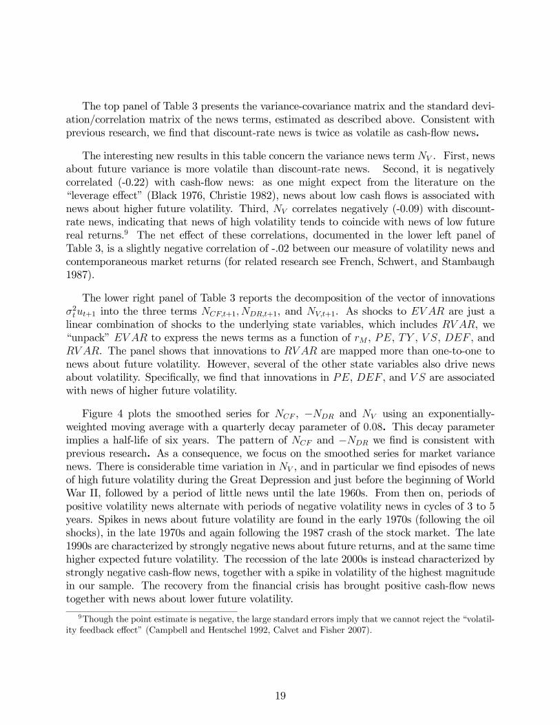
The top panel of Table 3 presents the variance-covariance matrix and the standard devi-

ation/correlation matrix of the news terms, estimated as described above. Consistent with

previous research, we find that discount-rate news is twice as volatile as cash-flow news.

The interesting new results in this table concern the variance news term . First, news

about future variance is more volatile than discount-rate news. Second, it is negatively

correlated (-0.22) with cash-flow news: as one might expect from the literature on the

“leverage effect” (Black 1976, Christie 1982), news about low cash flows is associated with

news about higher future volatility. Third, correlates negatively (-0.09) with discount-

rate news, indicating that news of high volatility tends to coincide with news of low future

real returns.9 The net effect of these correlations, documented in the lower left panel of

Table 3, is a slightly negative correlation of -.02 between our measure of volatility news and

contemporaneous market returns (for related research see French, Schwert, and Stambaugh

1987).

The lower right panel of Table 3 reports the decomposition of the vector of innovations

2+1 into the three terms +1 +1, and +1. As shocks to are just a

linear combination of shocks to the underlying state variables, which includes , we

“unpack” to express the news terms as a function of , , , , , and

. The panel shows that innovations to are mapped more than one-to-one to

news about future volatility. However, several of the other state variables also drive news

about volatility. Specifically, we find that innovations in , , and are associated

with news of higher future volatility.

Figure 4 plots the smoothed series for , − and using an exponentially-

weighted moving average with a quarterly decay parameter of 008. This decay parameter

implies a half-life of six years. The pattern of and − we find is consistent with

previous research. As a consequence, we focus on the smoothed series for market variance

news. There is considerable time variation in , and in particular we find episodes of news

of high future volatility during the Great Depression and just before the beginning of World

War II, followed by a period of little news until the late 1960s. From then on, periods of

positive volatility news alternate with periods of negative volatility news in cycles of 3 to 5

years. Spikes in news about future volatility are found in the early 1970s (following the oil

shocks), in the late 1970s and again following the 1987 crash of the stock market. The late

1990s are characterized by strongly negative news about future returns, and at the same time

higher expected future volatility. The recession of the late 2000s is instead characterized by

strongly negative cash-flow news, together with a spike in volatility of the highest magnitude

in our sample. The recovery from the financial crisis has brought positive cash-flow news

together with news about lower future volatility.

9Though the point estimate is negative, the large standard errors imply that we cannot reject the “volatil-

ity feedback effect” (Campbell and Hentschel 1992, Calvet and Fisher 2007).

19

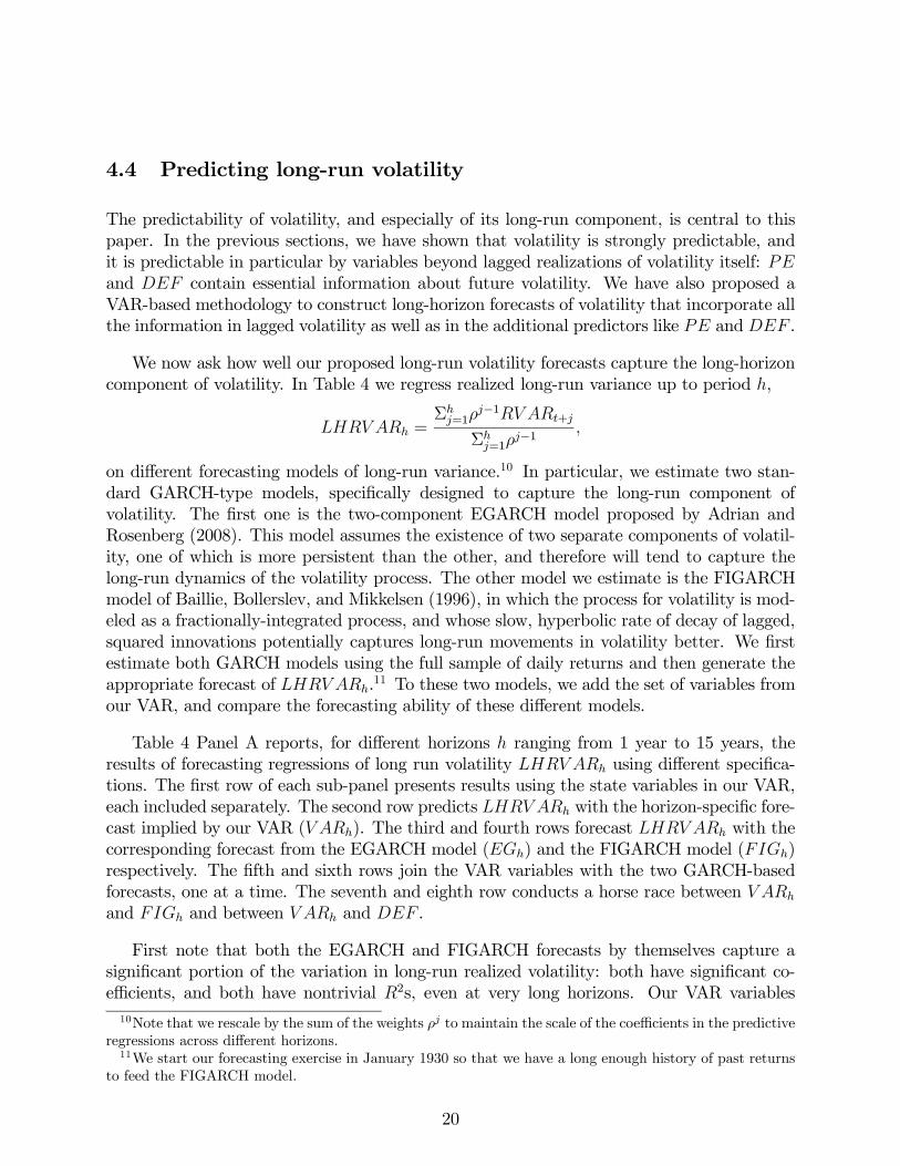
4.4 Predicting long-run volatility

The predictability of volatility, and especially of its long-run component, is central to this

paper. In the previous sections, we have shown that volatility is strongly predictable, and

it is predictable in particular by variables beyond lagged realizations of volatility itself:

and contain essential information about future volatility. We have also proposed a

VAR-based methodology to construct long-horizon forecasts of volatility that incorporate all

the information in lagged volatility as well as in the additional predictors like and .

We now ask how well our proposed long-run volatility forecasts capture the long-horizon

component of volatility. In Table 4 we regress realized long-run variance up to period ,

=Σ=1

−1 +

Σ=1

−1

on different forecasting models of long-run variance.10 In particular, we estimate two stan-

dard GARCH-type models, specifically designed to capture the long-run component of

volatility. The first one is the two-component EGARCH model proposed by Adrian and

Rosenberg (2008). This model assumes the existence of two separate components of volatil-

ity, one of which is more persistent than the other, and therefore will tend to capture the

long-run dynamics of the volatility process. The other model we estimate is the FIGARCH

model of Baillie, Bollerslev, and Mikkelsen (1996), in which the process for volatility is mod-

eled as a fractionally-integrated process, and whose slow, hyperbolic rate of decay of lagged,

squared innovations potentially captures long-run movements in volatility better. We first

estimate both GARCH models using the full sample of daily returns and then generate the

appropriate forecast of .11 To these two models, we add the set of variables from

our VAR, and compare the forecasting ability of these different models.

Table 4 Panel A reports, for different horizons ranging from 1 year to 15 years, the

results of forecasting regressions of long run volatility using different specifica-

tions. The first row of each sub-panel presents results using the state variables in our VAR,

each included separately. The second row predicts with the horizon-specific fore-

cast implied by our VAR ( ). The third and fourth rows forecast with the

corresponding forecast from the EGARCH model () and the FIGARCH model ()

respectively. The fifth and sixth rows join the VAR variables with the two GARCH-based

forecasts, one at a time. The seventh and eighth row conducts a horse race between

and and between and .

First note that both the EGARCH and FIGARCH forecasts by themselves capture a

significant portion of the variation in long-run realized volatility: both have significant co-

efficients, and both have nontrivial 2s, even at very long horizons. Our VAR variables

10Note that we rescale by the sum of the weights to maintain the scale of the coefficients in the predictive

regressions across different horizons.11We start our forecasting exercise in January 1930 so that we have a long enough history of past returns

to feed the FIGARCH model.

20

provide as good or better explanatory power, and , and appear strongly

statistically significant at all horizons (with the exception of at = 20, i.e. 5 years).

Finally, the VAR-implied forecast, , is not only significantly different from 0, but it is

also not significantly different from 1. This indicates that our VAR is able to produce fore-

casts of volatility that not only go in the right direction, but are also of the right magnitude,

even at very long horizons.

Very interesting results appear once we join our variables to the two GARCH models.

Even after controlling for the GARCH-based forecasts (which render insignificant),

and always come in significantly in predicting long-horizon volatility. Moreover,

and especially at long horizons, the addition of the VAR state variables strongly increases the

2. We further show that when using the VAR-implied forecast together with the FIGARCH

forecast, the coefficient on is still very close to one and always statistically significant

while the FIGARCH coefficient moves closer to zero (though estimates of the coefficient on

remain statistically significant at some horizons).

We develop an additional test of our VAR-based model of stochastic volatility from the

idea that the variables that form the VAR — in particular the strongest of them,

— should predict volatility at long horizons only through the VAR, not in addition to it.

In other words, the VAR forecasts should ideally represent the best way to combine the

information contained in the state variables concerning long-run volatility. If true, after

controlling for the VAR-implied forecast, DEF or other variables that enter the VAR should

not significantly predict future long-run volatility. We test this hypothesis by running a

regression using both the VAR-implied forecast and as right-hand side variables. We

find that at all horizons the coefficient on is still not significantly different from 1,

while the coefficient on is small and statistically indistinguishable from 0.

Finally, in Panel B of Table 4 we examine more carefully the link between and

focusing on the 10-year horizon. The Table reports the results from regressions

forecasting 40 with , ( orthogonalized to ), and

( orthogonalized to ). The Table shows that by itself, has no information about

low-frequency variation in volatility. In contrast, forecasts nearly 22% of the variation

in 40. And once is orthogonalized to , the 2 increases to 51%. Adding

has little effect on the 2. We argue that this is clear evidence of the strong predictive

power of the orthogonalized component of the default spread.

Recall our simple interpretation of these results. contains information about future

volatility as risky bonds are short the option to default. However, also contains

information about future aggregate risk premia. We know from previous work that most

of the variation in is about aggregate risk premia. Therefore, including in the

volatility forecasting regression cleans up variation in due to aggregate risk premia

and thus sharpens the link between and future volatility. Since and are

negatively correlated (default spreads are relatively low when the market trades rich), both

and receive positive coefficients in the multiple regression.

21

In Figure 5, we provide a visual representation of the volatility-forecasting power of

our key VAR state variables and our interpretation of the results. The top panel plots

40 together with lagged and . The graph confirms the strong negative

correlation between and (correlation of -0.6) and highlights how both variables

track long-run movements in long run volatility. To isolate the contribution of the default

spread in predicting long run volatility, the bottom panel plots 40 together with

. In general, the improvement in fit moving from the top panel to the bottom panel

is clear.

More specifically, the contrasting behavior of and in the two panels during

episodes such as the tech boom help illustrate the workings of our story. Taken in isola-

tion, the relatively stable default spread throughout most of the late 1990s would predict

little change in expectations of future market volatility. However, once the declining equity

premium over that period is taken into account (as shown by the rapid increase in ),

one recognizes that a -adjusted spread in the late 1990s actually forecasted much higher

volatility ahead.

Taken together, the results in Table 1 Panel A and Table 4 make a strong case that

credit spreads and valuation ratios contain information about future volatility not captured

by simple univariate models, even those like the FIGARCH model or the two-component

EGARCH model that are designed to fit long-run movements in volatility, and that our

VAR method for calculating long-horizon forecasts preserves this information.

5 Measuring and Pricing Cash-flow, Discount-Rate, and

Volatility Betas

5.1 Test assets

In addition to the six VAR state variables, our analysis also requires returns on a cross

section of test assets. We construct three sets of portfolios to use as test assets. Our primary

cross section consists of the excess returns on the 25 ME- and BE/ME-sorted portfolios,

studied in Fama and French (1993), extended in Davis, Fama, and French (2000), and made

available by Professor Kenneth French on his web site.12

Daniel and Titman (1997, 2012) and Lewellen, Nagel, and Shanken (2010) point out that

it can be misleading to test asset pricing models using only portfolios sorted by characteristics

known to be related to average returns, such as size and value. In particular, characteristics-

sorted portfolios are likely to show some spread in betas identified as risk by almost any asset

pricing model, at least in sample. When the model is estimated, a high premium per unit

12http://mba.tuck.dartmouth.edu/pages/faculty/ken.french/

22

of beta will fit the large variation in average returns. Thus, at least when premia are not

constrained by theory, an asset pricing model may spuriously explain the average returns to

characteristics-sorted portfolios.

To alleviate this concern, we follow the advice of Daniel and Titman (1997, 2012) and

Lewellen, Nagel, and Shanken (2010) and construct a second set of six portfolios double-

sorted on past risk loadings to market and variance risk. First, we run a loading-estimation

regression for each stock in the CRSP database where is the log stock return on stock

for month .

3X=1

+ = 0 +

3X=1

+ + ∆

3X=1

∆ + + +3

We calculate ∆ as a weighted sum of changes in the VAR state variables. The

weight on each change is the corresponding value in the linear combination of VAR shocks

that defines news about market variance. We choose to work with changes rather than shocks

as this allows us to generate pre-formation loading estimates at a frequency that is different

from our VAR. Namely, though we estimate our VAR using calendar-quarter-end data, our

approach allows a stock’s loading estimates to be updated at each interim month.

The regression is reestimated from a rolling 36-month window of overlapping observations

for each stock at the end of each month. Since these regressions are estimated from stock-level

instead of portfolio-level data, we use quarterly data to minimize the impact of infrequent

trading. With loading estimates in hand, each month we perform a two-dimensional sequen-

tial sort on market beta and ∆ beta. First, we form three groups by sorting stocks

on b . Then, we further sort stocks in each group to three portfolios on b∆ and record

returns on these nine value-weight portfolios. The final set of risk-sorted portfolios are the

two sets of three b portfolios within the extreme b∆ groups. To ensure that the aver-

age returns on these portfolio strategies are not influenced by various market-microstructure

issues plaguing the smallest stocks, we exclude the five percent of stocks with the lowest

from each cross-section and lag the estimated risk loadings by a month in our sorts.

In the empirical analysis, we consider two main subsamples: early (1931:3-1963:3) and

modern (1963:4-2011:4) due to the findings in Campbell and Vuolteenaho (2004) of dramatic

differences in the risks of these portfolios between the early and modern period. The first

subsample is shorter than that in Campbell and Vuolteenaho (2004) as we require each of

the 25 portfolios to have at least one stock as of the time of formation in June.

Finally, we generate a parsimonious cross section of option, bond, and equity returns for

the 1986:1-2011:4 time period based on the findings in Fama and French (1993) and Coval

and Shumway (2001). In particular, we use the S&P 100 index straddle returns studied by

Coval and Shumway.13 We also include proxies for the two components of the risky bond

13Specifically, the series we study includes only those straddle positions where the difference between the

23

factor of Fama and French (1993) which we measure using the return on the Barclays Capital

High Yield Bond Index ( ) and the return on Barclays Capital Investment Grade

Bond Index ( ). When pricing the straddle and risky bond return series, we include

the returns on the market ( ), size (), and value () equity factors of Fama

and French (1993) as they argue these factors do a good job describing the cross section of

average equity returns.

5.2 Beta measurement

We now examine the validity of an unconditional version of the first-order condition in

equation (18). We modify equation (18) in three ways. First, we use simple expected

returns on the left-hand side to make our results easier to compare with previous empirical

studies. Second, we condition down equation (18) to avoid having to estimate all required

conditional moments. Finally, we cosmetically multiply and divide all three covariances by

the sample variance of the unexpected log real return on the market portfolio. By doing so,

we can express our pricing equation in terms of betas, facilitating comparison to previous

research. These modifications result in the following asset-pricing equation

[ − ] = 2 + 2− 122 , (26)

where

≡ ( )

( −−1),

≡ (−)

( −−1),

and ≡ ( )

( −−1).

We price the average excess returns on our test assets using the unconditional first-order

condition in equation (26) and the quadratic relationship between the parameters and

given by (24). As a first step, we estimate cash-flow, discount-rate, and variance betas using

the fitted values of the market’s cash flow, discount-rate, and variance news estimated in

the previous section. Specifically, we estimate simple WLS regressions of each portfolio’s log

returns on each news term, weighting each time-+1 observation pair by the weights used to

estimate the VAR in Table 1 Panel B. We then scale the regression loadings by the ratio of

the sample variance of the news term in question to the sample variance of the unexpected

log real return on the market portfolio to generate estimates for our three-beta model.

options’ strike price and the underlying price is between 0 and 5. We thank Josh Coval and Tyler Shumway

for providing their updated data series to us.

24

Characteristic-sorted test assets

Table 5 Panel A shows the estimated betas for the 25 size- and book-to-market portfolios

over the 1931-1963 period. The portfolios are organized in a square matrix with growth

stocks at the left, value stocks at the right, small stocks at the top, and large stocks at the

bottom. At the right edge of the matrix we report the differences between the extreme growth

and extreme value portfolios in each size group; along the bottom of the matrix we report the

differences between the extreme small and extreme large portfolios in each BE/ME category.

The top matrix displays post-formation cash-flow betas, the middle matrix displays post-

formation discount-rate betas, while the bottom matrix displays post-formation variance

betas. In square brackets after each beta estimate we report a standard error, calculated

conditional on the realizations of the news series from the aggregate VAR model.

In the pre-1963 sample period, value stocks have both higher cash-flow and higher

discount-rate betas than growth stocks. An equal-weighted average of the extreme value

stocks across size quintiles has a cash-flow beta 0.12 higher than an equal-weighted average

of the extreme growth stocks. The difference in estimated discount-rate betas, 0.20, is in

the same direction. Similar to value stocks, small stocks have higher cash-flow betas and

discount-rate betas than large stocks in this sample (by 0.14 and 0.34, respectively, for an

equal-weighted average of the smallest stocks across value quintiles relative to an equal-

weighted average of the largest stocks). These differences are extremely similar to those in

Campbell and Vuolteenaho (2004), despite the exclusion of the 1929-1931 subperiod, the

replacement of the excess log market return with the log real return, and the use of a richer,

heteroskedastic VAR.

The new finding in Table 5 Panel A is that value stocks and small stocks are also riskier

in terms of volatility betas. An equal-weighted average of the extreme value stocks across

size quintiles has a volatility beta 0.21 lower than an equal-weighted average of the extreme

growth stocks. Similarly, an equal-weighted average of the smallest stocks across value

quintiles has a volatility beta that is 0.18 lower than an equal-weighted average of the largest

stocks. In summary, value and small stocks were unambiguously riskier than growth and

large stocks over the 1931-1963 period.

Table 6 Panel A reports the corresponding estimates for the post-1963 period. As doc-

umented in this subsample by Campbell and Vuolteenaho (2004), value stocks still have

slightly higher cash-flow betas than growth stocks, but much lower discount-rate betas. Our

new finding here is that value stocks continue to have much lower volatility betas, and the

spread in volatility betas is even greater than in the early period. The volatility beta for the

equal-weighted average of the extreme value stocks across size quintiles is 0.52 lower than

the volatility beta of an equal-weighted average of the extreme growth stocks, a difference

that is more than 42% higher than the corresponding difference in the early period.

One interesting aspect of these findings is the fact that the average of the 25 size-

and book-to-market portfolios changes sign from the early to the modern subperiod. Over

25

the 1931-1963 period, the average is -0.25 while over the 1964-2011 period this average

becomes 0.36. Of course, given the strong positive link between and volatility news

documented in the lower right panel of Table 3, one should not be surprised that the market’s

can be positive. Moreover, given the change in sign over time in ’s correlation with

some of the key state variables driving documented in the Online Appendix, one

should not be surprised that changes sign as well. Nevertheless, Table 12 examines the

robustness of this finding to different VAR specifications and estimation methods.

These results imply that in the post-1963 period where the CAPM has difficulty ex-

plaining the low returns on growth stocks relative to value stocks, growth stocks are relative

hedges for two key aspects of the investment opportunity set. Consistent with Campbell and

Vuolteenaho (2004), growth stocks hedge news about future real stock returns. The novel

finding of this paper is that growth stocks also hedge news about the variance of the market

return.

Risk-sorted test assets

Table 5 Panel B shows the estimated betas for the six risk-sorted portfolios over the

1931-1963 period. The portfolios are organized in a rectangular matrix with low CAPM

beta stocks at the left, high CAPM beta stocks at the right, low volatility beta stocks at

the top, and high volatility beta stocks at the bottom. At the right edge of the matrix we

report the differences between the high CAPM beta and the low CAPM beta portfolios in

each volatility beta group; along the bottom of the matrix we report the differences between

the high volatility beta and the low volatility beta portfolios in each CAPM beta category.

As in Panel A, the top matrix displays post-formation cash-flow betas, the middle matrix

displays post-formation discount-rate betas, while the bottommatrix displays post-formation

volatility betas.

In the pre-1963 sample period, high CAPM beta stocks have both higher cash-flow and

higher discount-rate betas than low CAPM beta stocks. An equal-weighted average of the

high CAPM beta stocks across the two volatility beta categories has a cash-flow beta 0.19

higher than an equal-weighted average of the low CAPM beta stocks. The difference in

estimated discount-rate betas is 0.44 and in the same direction. Similar to high CAPM beta

stocks, low volatility beta stocks have higher cash-flow betas and discount-rate betas than

high volatility beta stocks in this subsample (by 0.06 and 0.11, respectively, for an equal-

weighted average of the low volatility beta stocks across the three CAPM beta categories

relative to a corresponding equal-weighted average of the high volatility beta stocks).

High CAPM beta stocks and low volatility beta stocks are also riskier in terms of volatility

betas. An equal-weighted average of the high CAPM beta stocks across volatility beta

categories has a post-formation volatility beta 0.16 lower than an equal-weighted average of

the low CAPM beta stocks. Similarly, an equal-weighted average of the low volatility beta

stocks across CAPM beta categories has a post-formation volatility beta that is 0.09 lower

than an equal-weighted average of the high volatility beta stocks. In summary, high CAPM

26

beta and low volatility beta stocks were unambiguously riskier than low CAPM beta and

high volatility beta stocks over the 1931-1963 period.

Table 6 Panel B shows the estimated betas for the six risk-sorted portfolios over the

post-1963 period. In the modern period, high CAPM beta stocks again have higher cash-

flow and higher discount-rate betas than low CAPM beta stocks. An equal-weighted average

of the high CAPM beta stocks across the two volatility beta categories has a cash-flow beta

0.08 higher than an equal-weighted average of the low CAPM beta stocks. The difference in

estimated discount-rate betas is 0.55 and in the same direction. However, high CAPM beta

stocks are no longer riskier in terms of volatility betas. Now, an equal-weighted average of

the high CAPM beta stocks across the two volatility beta categories has a post-formation

variance beta 0.28 higher than a corresponding equal-weighted average of the low CAPM

beta stocks. Since, in the three-beta model, covariation with aggregate volatility has a

negative premium, the three-beta model can potentially explain why stocks with high past

CAPM betas have offered relatively little extra return, at least in the modern period.

In the post-1963 period, sorts on volatility beta continue to generate economically and

statistically significant spread in post-formation volatility beta. An equal-weighted average

of low volatility beta stocks across the three CAPM beta categories has a post-formation

volatility beta that is 0.26 lower than the post-formation volatility beta of a corresponding

equal-weighted average of high volatility beta stocks. Sorts on volatility beta also generate

spread in discount-rate beta, but essentially no spread in cash-flow betas in the post-1963

period.

Non-equity test assets

Finally, Table 6 Panel C reports the three ICAPM betas of the S&P 100 index straddle

position analyzed in Coval and Shumway (2001) along with the corresponding ICAPM betas

of the three equity factors and the default bond factor of Fama and French (1993) over the

period 1986:1 - 2011:4. Consistent with the nature of a straddle bet, we find that the straddle

has a very large volatility beta of 1.51 along with a large negative discount-rate beta of -1.71

and a large (relatively speaking) negative cash-flow beta of -0.39. As one would expect, the

betas of the Fama-French equity factors are consistent with the findings for the size- and

book-to-market-sorted portfolios in Table 6 Panel B. Finally, the riskier component of Fama

and French’s (1993) risky bond factor, , has a cash-flow beta of 0.06, a discount-rate

beta of 0.26, and a volatility beta of -0.20. These betas are economically and statistically

significant from those of the safer component, . The difference in volatility beta

between and is consistent with the fact that risky corporate debt is short

the option to default.

27

5.3 Beta pricing

We next turn to pricing the cross section with these three ICAPM betas. We evaluate

the performance of five asset-pricing models: 1) the traditional CAPM that restricts cash-

flow and discount-rate betas to have the same price of risk and sets the price of variance risk

equal to zero; 2) the two-beta intertemporal asset pricing model of Campbell and Vuolteenaho

(2004) that restricts the price of discount-rate risk to equal the variance of the market return,

3) our three-beta intertemporal asset pricing model that restricts the price of discount-rate

risk to equal the variance of the market return and constrains the price of cash-flow and

variance risk to be related by equation (24), with = 095 per year; 4) a partially-constrained

three-beta model that restricts the price of discount-rate risk to equal the variance of the

market return but freely estimates the other two risk prices (effectively decoupling and ),

and 5) an unrestricted three-beta model that allows free risk prices for cash-flow, discount-

rate, and volatility betas. Each model is estimated in two different forms: one with a

restricted zero-beta rate equal to the Treasury-bill rate, and one with an unrestricted zero-

beta rate following Black (1972).

Characteristic-sorted test assets

Table 7 reports results for the early sample period 1931-1963, using 25 size- and book-

to-market-sorted portfolios as test assets. The table has ten columns, two specifications for

each of our five asset pricing models. The first 16 rows of Table 7 are divided into four sets

of four rows. The first set of four rows corresponds to the zero-beta rate (in excess of the

Treasury-bill rate), the second set to the premium on cash-flow beta, the third set to the

premium on discount-rate beta, and the fourth set to the premium on volatility beta. Within

each set, the first row reports the point estimate in fractions per quarter, and the second

row annualizes this estimate, multiplying by 400 to aid in interpretation. These parameters

are estimated from a cross-sectional regression

= 0 + 1b + 2b+ 3b + (27)

where a bar denotes time-series mean and

≡ − denotes the sample average simple

excess return on asset . The third and fourth rows present two alternative standard errors

of the monthly estimate, described below.

Below the premia estimates, we report the 2 statistic for a cross-sectional regression of

average returns on our test assets onto the fitted values from the model. We also report a

composite pricing error, computed as a quadratic form of the pricing errors. The weighting

matrix in the quadratic form is a diagonal matrix with the inverse of the sample test asset

return volatilities on the main diagonal.

Standard errors are produced with a bootstrap from 10,000 simulated realizations. Our

bootstrap experiment samples test-asset returns and first-stage VAR errors, and uses the

first-stage and second-stage WLS VAR estimates in Table 1 to generate the state-variable

28

data.14 We partition the VAR errors and test-asset returns into two groups, one for 1931 to

1963 and another for 1963 to 2011, which enables us to use the same simulated realizations

in subperiod analyses. The first set of standard errors (labeled A) conditions on estimated

news terms and generates betas and return premia separately for each simulated realization,

while the second set (labeled B) also estimates the first-stage and second-stage VAR and the

news terms separately for each simulated realization. Standard errors B thus incorporate

the considerable additional sampling uncertainty due to the fact that the news terms as well

as betas are generated regressors.

Two alternative 5-percent critical values for the composite pricing error are produced

with a bootstrap method similar to the one we have described above, except that the test-

asset returns are adjusted to be consistent with the pricing model before the random samples

are generated. Critical values A condition on estimated news terms, while critical values B

take account of the fact that news terms must be estimated.

Finally, Table 7 reports the implied risk-aversion coefficient, , which can be recovered as

12, as well as the sensitivity of news about risk to news about market variance, , which

can be recovered as −2 ∗ 32. The three-beta ICAPM estimates are constrained so that

both and the implied are strictly positive.

Table 7 shows that in the 1931-1963 period, the restricted three-beta model explains the

cross-section of stock returns reasonably well. The cross-sectional 2 statistics are almost

56% for both forms of this model. Both the Sharpe-Lintner and Black versions of the CAPM

do a slightly poorer job describing the cross section (both 2 statistics are roughly 52%).

The two-beta ICAPM of Campbell and Vuolteenaho (2004) performs slightly better than the

CAPM and slightly worse than the volatility ICAPM. None of the theoretically-motivated

models considered are rejected by the data based on the composite pricing test. Consistent

with the claim that the three-beta model does a good job describing the cross-section, Table 7

shows that the constrained and the unrestricted factor model barely improve pricing relative

to the three-beta ICAPM.

Figure 6 provides a visual summary of these results. The figure plots the predicted

average excess return on the horizontal axis and the actual sample average excess return on

the vertical axis. In summary, we find that the three-beta ICAPM improves pricing relative

to both the Sharpe-Lintner and Black versions of the CAPM.

This success is due in part to the inclusion of volatility betas in the specification. For the

Black version of the three-beta ICAPM, the spread in volatility betas across the 25 size- and

book-to-market-sorted portfolios generates an annualized spread in average returns of 1.46%

compared to a comparable spread of 7.41% and 3.18% for cash-flow and discount-rate betas.

Variation in volatility betas accounts for 2% of the variation in explained returns compared

to 39% and 7% for cash-flow and discount-rate betas respectively. The remaining 52% of the

explained variation in average returns is due of course to the covariation among the three

14When simulating the bootstrap, we drop realizations which would result in negative and redraw.

29

types of betas.

Results are very different in the 1963-2011 period. Table 8 shows that in this period,

both versions of the CAPM do a very poor job of explaining cross-sectional variation in

average returns on portfolios sorted by size and book-to-market. When the zero-beta rate

is left as a free parameter, the cross-sectional regression picks a negative premium for the

CAPM beta and implies an 2 of roughly 5%. When the zero-beta rate is constrained to

the risk-free rate, the CAPM 2 falls to roughly -37%. Both versions of the static CAPM

are easily rejected at the five-percent level by both sets of critical values.

In the modern period, the unconstrained zero-beta rate version of the two-beta Campbell

and Vuolteenaho (2004) model does a better job describing the cross section of average

returns than the CAPM. However, the implied coefficient of risk aversion, 20.70, is arguably

extreme.

The three-beta model with the restricted zero-beta rate also does a poor job explaining

cross-sectional variation in average returns across our test assets. However, if we continue

to restrict the risk price for discount-rate and variance news but allow an unrestricted zero-

beta rate, the explained variation increases to roughly 69%, three-quarters larger than the

2 of the corresponding two-beta ICAPM. The estimated risk price for cash-flow beta is

an economically reasonable 30 percent per year with an implied coefficient of relative risk

aversion of 9.63. Both versions of our intertemporal CAPM with stochastic volatility are not

rejected at the 5-percent level by either set of critical values.

Figure 7 provides a visual summary of these results. For the Black version of the three-

beta ICAPM, spread in volatility betas across the 25 size- and book-to-market-sorted port-

folios generates an annualized spread in average returns of 6.52% compared to a comparable

spread of 3.90% and 2.24% for cash-flow and discount-rate betas. Variation in volatility

betas accounts for 92% of the variation in explained returns compared to 20% for cash-flow

betas as well as 7% for discount-rate betas. Covariation among the three types of betas is

responsible for the remaining -19% of explained variation in average returns.

The relatively poor performance of the risk-free rate version of the three-beta ICAPM is

due to the derived link between and . To show this, Figure 8 provides two contour plots

(one each for the risk-free and zero-beta rate versions of the model in the top and bottom

panels of the figure respectively) of the 2 resulting from combinations of (,) ranging from

(0,0) to (40,16). On the same figure we also plot the relation between and derived in

equation (24). The top panel of Figure 8 shows that even with the intercept restricted to

zero, 2’s are as high as 70% for some combinations of (,). Unfortunately, as the plot

shows, these combinations do not coincide with the curve implied by equation (24). Once

the zero-beta rate is unconstrained, the contours for 2’s greater than 60% cover a much

larger area of the plot and coincide nicely with the ICAPM relation of equation (24).

Consistent with the contour plots of Figure 8, the pricing results in Table 8 based on

the partially-constrained factor model further confirms that the link between and is

30

responsible for the poor fit of the restricted zero-beta rate version of the three-beta ICAPM

in the modern period. When removing the constraint linking and but leaving the

constraint on the discount-rate beta premium in place, the 2 increases from -57% to 74%.

Nevertheless, the risk prices for and remain economically large and of the right sign.

Risk-sorted test assets

We confirm that the success of the three-beta ICAPM is robust by expanding the set of

test portfolios beyond the 25 size- and book-to-market-sorted portfolios. First, we show that

our three-beta model not only describes the cross section of characteristics-sorted portfolios

but also can explain the average returns on risk-sorted portfolios. We examine risk-sorted

portfolios as Daniel and Titman (1997, 2012) and Lewellen, Nagel, and Shanken (2010) argue

that asset-pricing tests using only portfolios sorted by characteristics known to be related to

average returns, such as size and value, can be misleading due to the low-dimensional factor

structure of the 25 size and book-to-market-sorted portfolios.

Table 9 prices the six risk-sorted portfolios described in Table 5 Panel B in conjunction

with six of the 25 size- and book-to-market-sorted portfolios of Table 5 Panel A (the low,

medium, and high BE/ME portfolios within the small and large ME quintiles). We continue

to find that the three-beta ICAPM improves pricing relative to both the Sharpe-Lintner and

Black versions of the CAPM. Moreover, the relatively high2 (57%) is not disproportionately

due to characteristics-sorted portfolios as the 2 for the risk-sorted subset (69%) is not only

comparable to but also larger than the 2 for the characteristics-sorted subset (51%). Figure

9 shows this success graphically.

Table 10 prices the cross section of characteristics- and risk-sorted portfolios in the mod-

ern period. We find that the zero-beta rate three-beta ICAPM is not rejected by the data

while both versions of the CAPM are rejected. Again, the relatively high 2 for the zero-beta

rate version of the volatility ICAPM (76%) is not disproportionately due to characteristics-

sorted portfolios as the 2 for the risk-sorted subset (81%) is not only comparable to but

also larger than the 2 for the characteristics-sorted subset (77%). Figure 10 provides a

graphically summary of these results.

Non-equity test assets

We also show that our three-beta model can help explain average returns on non-equity

portfolios designed to be highly correlated with aggregate volatility risk, namely the S&P

100 index straddles of Coval and Shumway (2001). We first calculate the expected return on

straddle portfolio based on the estimates of the zero-beta rate volatility ICAPM in Table 8.

The contributions to expected quarterly return from the straddle’s cash-flow, discount-rate,

and volatility betas are -2.92%, -1.33%, and -3.87% respectively. As the average quarterly

realized return on the straddle is -21.66%, an equity-based estimate of the three-beta model

explains roughly 38% of the realized straddle premium.

Table 11 shows that our intertemporal CAPM with stochastic volatility is not rejected at

31

the 5-percent level when we price the joint cross-section of equity, bond, and straddle returns.

The implied risk aversion coefficient (roughly 15 for both the risk-free and zero-beta rate

implementations of the model) is high but not unreasonable. In sharp contrast, the CAPM

is strongly rejected. Though the two-beta ICAPM is not rejected, the required risk aversion

is too extreme (over 53 for both versions of the model) to be realistic.

Summary of US financial history

Figure 11 (third panel) plots the time-series of the smoothed combined shock − − 1

2 based on the estimate of the zero-beta model for the modern period (Table

7). The correlation of this shock with the associated is 0.90. Similarly, the correlation

of this shock with the associated is 0.26. Finally, the correlation of this shock with the

associated is -0.76. Figure 11 also plots the corresponding smoothed shock series for the

CAPM ( − ) and for the two-beta ICAPM ( − ). The two-beta model

shifts the history of good and bad times relative to the CAPM, as emphasized by Campbell,

Giglio, and Polk (2012). The model with stochastic volatility further accentuates that

periods with high market volatility, such as the 1930s and the late 2000s, are particularly

hard times for long-term investors.

5.4 Robustness

Table 12 examines the robustness of our findings. Where appropriate, we include in bold

font our baseline model as a benchmark. Panel A shows results using various subsets of

variables in our baseline VAR. These results indicate that including both and are

generally essential for our finding of a negative for , consistent with the importance

of these two variable to long-run volatility forecasting. Moreover, successful zero-beta-rate

volatility ICAPM pricing in the modern period requires , , and in the VAR. The

results in Panel A also show that the positive in the modern period is due to the

inclusion of and in the VAR. This finding makes sense once one is convinced (and

the long-horizon regressions of Table 4 make a strong case) that, controlling for , high

forecasts high volatility in the future. Since the market will certainly covary positively

(and quite strongly) with the shock, one should expect this component of volatility news

to be positive and an important determinant of ’s .

Panel B presents results based on different estimation methods for the VAR. These meth-

ods include OLS, WLS but with OLS betas, two different bounds on the maximum ratio of

WLS weights, a single-stage approach where the weights are proportional to rather

than , and a partial VAR where we throw out in each regression those variables with -

statistics under 1.0 (in an iterative fashion, starting with the weakest -statistic first). These

results show that our major findings (a negative for and successful zero-beta rate

ICAPM pricing in both time periods) are very robust to using different methods.

In Panel C, we augment the set of variables under consideration to be included in the

32

VAR. We first explore different ways to measure the market’s valuation ratio. In the second

column of the Table, we replace with Re where we construct the price-earnings

ratio by deflating both the price and the earnings series by the CPI before taking their

ratio. In the third column, we use the log price-dividend ratio, , instead of . In

column four, we replace with Re and the CPI inflation rate, . Panel C also

explores adding two additional state variables. In column five, we add (Lettau and

Ludvigson (2001)) to the VAR as is known to be a strong predictor of future market

returns. Finally, column six adds the quarterly forecast to the VAR as Table

4 Panel B documents that GARCH-based methods are useful predictors of future market

return variance. In total, this Panel confirms that our finding of a negative for and

successful zero-beta rate ICAPM pricing in both time periods is generally robust to these

variations.

Panel D reports the results when we vary the excess zero-beta rate. One might argue that

our excess zero-beta rate estimate of 86 basis points a quarter is too high to be consistent

with equilibrium. Fortunately, we find that 2s remain reasonable for excess zero-beta rates

that are as low as 40 bps/quarter.

Panels E and F present information to help us better understand the volatility betas we

have estimated for the market as a whole, and for value stocks relative to growth stocks.

Panel E reports components of and’s in each period (estimated either with

WLS or OLS). Specifically, these results use the elements of the vector defined in equation

(17) and the corresponding VAR shock to measure how each shock contributes to the in

question. Panel E documents, consistent with Panel A, that has a positive in

the modern period due in part to the state variable. The results in Panel E also show

that all of the non-zero components of ’s in the modern period are negative. This

finding is comforting as it further confirms that our negative beta finding is robust.

Panel E also reports OLS estimates of simple betas on and the 15-year horizon

forecast (60) for and . The betas based on these two

simple proxies have the same sign as our more sophisticated and more appropriate measure

of volatility news. However, conclusions about the relevance of volatility risk for the value

effect clearly depend on measuring the long-run component of volatility well.

Finally, Panel F reports time-series regressions of on by itself as well as on

all three factors together. We find that explains over 20% of ’s returns in the

modern period. The three news factors together explain slightly over 28%. Thus our model

is able to explain not only the cross-sectional variation in average returns of the 25 size- and

book-to-market-sorted portfolios of Fama and French (1993) but also a significant amount

of time series variation in realized returns on the key factor that they argue is multifactor-

minimum-variance (Fama and French, 1996).

33

6 Conclusion

We extend the approximate closed-form intertemporal capital asset pricing model of Camp-

bell (1993) to allow for stochastic volatility. Our model recognizes that an investor’s invest-

ment opportunities may deteriorate either because expected stock returns decline or because

the volatility of stock returns increases. A conservative long-term investor will wish to hedge

against both types of changes in investment opportunities; thus, a stock’s risk is determined

not only by its beta with unexpected market returns and news about future returns (or

equivalently, news about market cash flows and discount rates), but also by its beta with

news about future market volatility. Although our model has three dimensions of risk, the

prices of all these risks are determined by a single free parameter, the coefficient of relative

risk aversion.

Our implementation models the return on the aggregate stock market as one element

of a vector autoregressive (VAR) system; the volatility of all shocks to the VAR is another

element of the system. The empirical implementation of our VAR reveals new low-frequency

movements in market volatility tied to the default spread. We show that the negative

post-1963 CAPM alphas of growth stocks are justified because these stocks hedge long-

term investors against both declining expected stock returns, and increasing volatility. The

addition of volatility risk to the model helps it to deliver a moderate, economically reasonable

value of risk aversion.

Our empirical work is limited in one important respect. We test only the unconditional

implications of the model and do not evaluate its conditional implications. A full conditional

test is likely to be a challenging hurdle for the model. To see why, recall that we assume

a rational long-term investor always holds 100% of his or her assets in equities. However,

time-variation in real stock returns generally gives the long-term investor an incentive to

shift the relative weights on cash and equity, unless real interest rates and market volatility

move in exactly the right way to make the equity premium proportional to market volatility.

Although we do not explicitly test whether this is the case, previous work by Campbell

(1987) and Harvey (1989, 1991) rejects this proportionality restriction.

One way to support the assumption of constant 100% equity investment is to invoke

binding leverage constraints. Indeed, in the modern sample, the Black (1972) version of our

three-beta model is consistent with this interpretation as the estimated difference between

the zero-beta and risk-free rates is positive, statistically significant, and economically large.

However, the risk aversion coefficient we estimate may be too large to explain why leverage

constraints should bind.

Nevertheless, our model does directly answer the interesting microeconomic question: Are

there reasonable preference parameters that would make a long-term investor, constrained

to invest 100% in equity, content to hold the market rather than tilting towards value stocks

or other high-return stock portfolios? Our answer is clearly yes.

34

Appendix

Deriving the equation for

Here we show how to solve for the unknown parameter as discussed in section 3. We

start from the definition of

2 = Var [+1 + +1]

= Var

∙

+1 + (1− )+1

¸= Var

∙

µ( − 1)+1 +

1

2

+1

¶+ (1− )+1

¸= Var

∙(1− )+1 +

1

2+1 + (1− )+1

¸= Var

∙(1− )+1 +

1

2+1

¸= (1− )2Var

£+1

¤+ (1− )Cov

£+1+1

¤+

2

4Var

£+1

¤

deriving equation (19). Since cash flow and volatility news can be expressed in terms of the

VAR parameters as

+1 = 02( − Γ)−1+1+1 = (01 + 01Γ( − Γ)−1)+1

we can define the covariance matrix of VAR shocks as Σ =Var [+1] =Var[+1] and the

error-to-news vectors and defined in equations (20) and (21), to write as the

solution to

0 = 21

4Σ

0 − (1− (1− )Σ

0 ) + (1− )

2Σ

0

as was presented in equation (22)

Selecting the correct root of the quadratic equation

The equation defining will generally have two solutions

=1− (1− )Σ

0 ±

q(1− (1− )Σ

0 )2 − (1− )

2(Σ

0 ) (Σ

0 )

12Σ

0

As was discussed in the paper, this is an artifact of the loglinear approximation. While the

(approximate) Euler equation holds for both roots, the correct solution is the one with the

negative sign on the radical shown in equation (23).

35

This can be confirmed from numerical computation, and it can also be easily seen by

observing the behavior of the solutions in the limit as volatility news goes to zero and the

model become homoskedastic. With the false solution, becomes infinitely large as → 0.

This corresponds to the log value of invested wealth going to negative infinity. On the other

hand, we can use the correct solution for converges to (1− )2Σ

0 . This is what we

would expect, since in that case = 1Var [(1− )+1].

An approximation for

As discussed in section 3, we will not find a real solution for if

(1− )2(Σ

0 ) (Σ

0 ) (1− (1− )Σ

0 )2

This an unfortunate artifact of the loglinearization approach, as the conditional variance

defining =Var

h+1++1

iwill be real and finite for the true stochastic discount factor,

+1. We propose an alternative approach that will allow us to approximate even when

64, the region where there is no real solution given our estimated VAR parameters.

We start from the definition of

=1

2Var

∙(1− )+1 +

1

2+1

¸= 2

1

4Σ

0 + (1− )Σ

0 + (1− )

2Σ

0

and approximate the variance term on the right hand side so that it is a linear function of

rather than quadratic. Taking a Taylor approximation about = 0

≈ (1− )2Σ

0 + (1− )Σ

0

where the first term on the right hand side is the traditional value that we would see in

the homoskedastic case, as pointed out in the text. The second term is the additional effect

coming from stochastic volatility. Now, solving for we generate the approximation used

in the empirical analysis.

≈ (1− )2Σ

0

1− (1− )Σ0

36

References

Adrian, Tobias and Joshua Rosenberg, 2008, “Stock Returns and Volatility: Pricing the

Short-Run and Long-Run Components of Market Risk”, Journal of Finance 63:2997—

3030.

Andersen, Torben G., Tim Bollerslev, Francis X. Diebold, and Paul Labys, 2003, “Modeling

and Forecasting Realized Volatility”, Econometrica 71:579—625.

Andersen, Torben, Tim Bollerslev, Peter F. Christoffersen and Francis X. Diebold, 2006,

“Volatility and Correlation Forecasting”, in Graham Elliott, Clive W.J. Granger and

Allan Timmermann (eds), Handbook of Economic Forecasting, Vol I.

Ang, Andrew, Robert J. Hodrick, Yuhang Xing, and Xiaoyan Zhang, 2006, “The Cross-

Section of Volatility and Expected Returns”, Journal of Finance 61:259—299.

Baillie, Richard T., Tim Bollerslev and Hans Ole Mikkelsen, 1996, “Fractionally integrated

generalized autoregressive conditional heteroskedasticity”, Journal of Econometrics

74:3—30.

Bansal, Ravi and Amir Yaron, 2004, “Risks for the Long Run”, Journal of Finance 59:1481—

1509.

Bansal, Ravi, Dana Kiku and Amir Yaron, 2012, “An Empirical Evaluation of the Long-Run

Risks Model for Asset Prices”, Critical Finance Review 1:183—221.

Bansal, Ravi, Dana Kiku, Ivan Shaliastovich and Amir Yaron, 2012, “Volatility, the Macro-

economy and Asset Prices”, unpublished paper, Duke University and University of

Pennsylvania.

Barndorff-Nielsen, Ole E. and Neil Shephard, 2002, “Econometric Analysis of Realized

Volatility and Its Use in Estimating Stochastic Volatility Models”, Journal of the Royal

Statistical Society B, 64(2):253—280.

Beeler, Jason and John Y. Campbell, 2012, “The Long-Run Risks Model and Aggregate

Asset Prices: An Empirical Assessment”, Critical Finance Review 1:141-182.

Black, Fisher, 1972, “Capital Market Equilibrium with Restricted Borrowing”, Journal of

Business 45:444—454.

Black, Fisher, 1976, “Studies of Stock Price Volatility Changes”, Proceedings of the 1976

Meetings of the American Statistical Association, Business and Economic Statistics

Section, Washington 177-181.

Bollerslev, Tim, 1986, “Generalized Autoregressive Conditional Heteroskedasticity”, Jour-

nal of Econometrics 31, 307—327.

37

Breeden, Douglas T., 1979, “An Intertemporal Asset Pricing Model with Stochastic Con-

sumption and Investment Opportunities”, Journal of Financial Economics 7:265—296.

Calvet, Laurent and Adlai Fisher, 2007, “Multifrequency News and Stock Returns”, Journal

of Financial Economics 86:178—212.

Campbell, John Y., 1987, “Stock Returns and the Term Structure”, Journal of Financial

Economics 18:373—399.

Campbell, John Y., 1993, “Intertemporal Asset Pricing Without Consumption Data”,

American Economic Review 83:487—512.

Campbell, John Y., 1996, “Understanding Risk and Return”, Journal of Political Economy

104:298—345.

Campbell, John Y., Stefano Giglio, and Christopher Polk, 2012, “Hard Times”, unpublished

paper, Harvard University, University of Chicago, and London School of Economics.

Campbell, John Y., Stefano Giglio, Christopher Polk, and Robert Turley, 2012, “Internet

Appendix to An Intertemporal CAPM with Stochastic Volatility”, available online at

http://kuznets.fas.harvard.edu/~campbell/papers.html.

Campbell, John Y. and Ludger Hentschel, 1992, “No News is Good News: An Asymmet-

ric Model of Changing Volatility in Stock Returns”, Journal of Financial Economics

31:281—318.

Campbell, John Y., Christopher Polk, and Tuomo Vuolteenaho, 2010, “Growth or Glamour?

Fundamentals and Systematic Risk in Stock Returns” Review of Financial Studies

23:305—344.

Campbell, John Y. and Robert J. Shiller, 1988a, “The Dividend-Price Ratio and Expecta-

tions of Future Dividends and Discount Factors”, Review of Financial Studies 1:195—

228.

Campbell, John Y. and Robert J. Shiller, 1988b, “Stock Prices, Earnings, and Expected

Dividends”, Journal of Finance 43:661—676.

Campbell, John Y. and Glen B. Taksler, 2003, “Equity Volatility and Corporate Bond

Yields”, Journal of Finance 58:2321—2349.

Campbell, John Y. and Tuomo Vuolteenaho, 2004, “Bad Beta, Good Beta”, American

Economic Review 94:1249—1275.

Chacko, George and Luis M. Viceira, 2005, “Dynamic Consumption and Portfolio Choice

with Stochastic Volatility in Incomplete Markets”, Review of Financial Studies 18:1369—

1402.

38

Chen, Joseph, 2003, “Intertemporal CAPM and the Cross Section of Stock Returns”, un-

published paper, University of California Davis.

Chen, Long and Xinlei Zhao, 2009, “Return Decomposition”, Review of Financial Studies

22:5213—5249.

Christiansen, Charlotte, Maik Schmeling and Andreas Schrimpf, 2012, “A Comprehensive

Look at Financial Volatility Prediction by Economic Variables”, BIS Working Paper

374.

Christie, Andrew, “The Stochastic Behavior of Common Stock Variances — Value, Leverage,

and Interest Rates Effects”, Journal of Financial Economics 10:407—432.

Cochrane, John H., 2008, “The Dog That Did Not Bark: A Defense of Return Predictabil-

ity”, Review of Financial Studies 21:1533-1575.

Cochrane, John H., 2011, “Presidential Address: Discount Rates”, Journal of Finance

66:1047—1108.

Coval, Josh, and Tyler Shumway, 2001, “Expected Option Returns”, Journal of Finance

56:983—1009.

Daniel, Kent and Sheridan Titman, 1997, “Evidence on the Characteristics of Cross-

sectional Variation in Common Stock Returns”, Journal of Finance 52:1—33.

Daniel, Kent and Sheridan Titman, 2012, “Testing Factor-Model Explanations of Market

Anomalies”, Critical Finance Review 1:103—139.

Davis, James L., Eugene F. Fama, and Kenneth R. French, “Characteristics, Covariances,

and Average Returns: 1929 to 1997”, Journal of Finance 55:389—406.

Duffee, Greg, 2005, “Time-Variation in the Covariance Between Stock Returns and Con-

sumption Growth”, Journal of Finance 60:1673—172.

Engle, Robert F, 1982, “Autoregressive Conditional Heteroscedasticity with Estimates of

the Variance of United Kingdom Inflation,” Econometrica 50:987—1007.

Engle, Robert F., Eric Ghysels and Bumjean Sohn, 2009, “Stock Market Volatility and

Macroeconomic Fundamentals”, unpublished paper, New York University, University

of North Carolina, and Georgetown University.

Engsted, Tom, Thomas Q. Pedersen, and Carsten Tanggaard, 2010, “Pitfalls in VAR Based

Return Decompositions: A Clarification”, unpublished paper, University of Aarhus.

Epstein, Lawrence and Stanley Zin, 1989, “Substitution, Risk Aversion, and the Temporal

Behavior of Consumption and Asset Returns: A Theoretical Framework”, Economet-

rica 57:937—69.

39

Eraker, Bjorn, 2008, “Affine General Equilibrium Models”, Management Science 54:2068—

2080.

Eraker, Bjorn and Ivan Shaliastovich, 2008, “An Equilibrium Guide to Designing Affine

Pricing Models”, Mathematical Finance 18:519—543.

Eraker, Bjorn and Wenyu Wang, 2011, “Dynamic Present Values and the Intertemporal

CAPM”, University of Wisconsin working paper.

Fama, Eugene F. and Kenneth R. French, 1993, Common risk factors in the returns on

stocks and bonds, Journal of Financial Economics 33, 3—56.

Fama, Eugene F. and Kenneth R. French, 1996, Multifactor Explanations of Asset Pricing

Anomalies, Journal of Finance 51, 55—84.

French, Ken, William Schwert, and Robert Stambaugh, 1987, “Expected stock returns and

volatility”, Journal of Financial Economics 19:3—29.

Harvey, Campbell, 1989, “Time-Varying Conditional Covariances in Tests of Asset Pricing

Models”, Journal of Financial Economics 24:289—317.

Harvey, Campbell, 1991, “TheWorld Price of Covariance Risk”, Journal of Finance 46:111—

157.

Kandel, Shmuel and Robert Stambaugh, 1991, “Asset Returns and Intertemporal Prefer-

ences”, Journal of Monetary Economics 27:39—71.

Lewellen, Jonathan, Stefan Nagel, and Jay Shanken, 2010, “A Skeptical Appraisal of Asset

Pricing Tests”, Journal of Financial Economics 96:175—194.

Liu, Jun, 2007, “Portfolio Selection in Stochastic Environments”, Review of Financial Stud-

ies 20:1—39.

Merton, Robert C., 1973, “An Intertemporal Capital Asset Pricing Model”, Econometrica

41:867—87.

Paye, Bradley, 2012, “Deja Vol: Predictive Regressions for Aggregate Stock Market Volatil-

ity using Macroeconomic Variables”, unpublished paper, University of Georgia.

Poon, Ser-Huang, and Clive W. J. Granger, 2003, “Forecasting Volatility in Financial

Markets: A Review”, Journal of Economic Literature 41:478—539

Restoy, Ferdo, and Philippe Weil, 1998, “Approximate Equilibrium Asset Prices”, NBER

Working Paper 6611.

Restoy, Ferdo, and Philippe Weil, 2011, “Approximate Equilibrium Asset Prices”, Review

of Finance 15:1—28.

40

Schwert, William, 1989, “Why Does Stock Market Volatility Change Over Time?”, Journal

of Finance 44:1115—1153.

Sohn, Bumjean, 2010, “Stock Market Volatility and Trading Strategy Based Factors”, un-

published paper, Georgetown University.

Tauchen, George and Robert Hussey, 1991, “Quadrature-Based Methods for Obtaining

Approximate Solutions to Nonlinear Asset Pricing Models”, Econometrica 59:317—96.

41

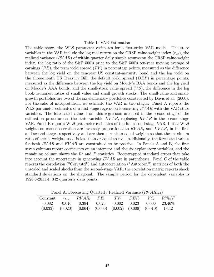
Table 1: VAR Estimation

The table shows the WLS parameter estimates for a first-order VAR model. The state

variables in the VAR include the log real return on the CRSP value-weight index (), the

realized variance ( ) of within-quarter daily simple returns on the CRSP value-weight

index, the log ratio of the S&P 500’s price to the S&P 500’s ten-year moving average of

earnings (), the term yield spread ( ) in percentage points, measured as the difference

between the log yield on the ten-year US constant-maturity bond and the log yield on

the three-month US Treasury Bill, the default yield spread ( ) in percentage points,

measured as the difference between the log yield on Moody’s BAA bonds and the log yield

on Moody’s AAA bonds, and the small-stock value spread ( ), the difference in the log

book-to-market ratios of small value and small growth stocks. The small-value and small-

growth portfolios are two of the six elementary portfolios constructed by Davis et al. (2000).

For the sake of interpretation, we estimate the VAR in two stages. Panel A reports the

WLS parameter estimates of a first-stage regression forecasting with the VAR state

variables. The forecasted values from this regression are used in the second stage of the

estimation procedure as the state variable , replacing in the second-stage

VAR. Panel B reports WLS parameter estimates of the full second-stage VAR. Initial WLS

weights on each observation are inversely proportional to and in the first

and second stages respectively and are then shrunk to equal weights so that the maximum

ratio of actual weights used is less than or equal to five. Additionally, the forecasted values

for both and are constrained to be positive. In Panels A and B, the first

seven columns report coefficients on an intercept and the six explanatory variables, and the

remaining column shows the 2 and statistics. Bootstrapped standard errors that take

into account the uncertainty in generating are in parentheses. Panel C of the table

reports the correlation ("Corr/std") and autocorrelation ("Autocorr.") matrices of both the

unscaled and scaled shocks from the second-stage VAR; the correlation matrix reports shock

standard deviations on the diagonal. The sample period for the dependent variables is

1926.3-2011.4, 342 quarterly data points.

Panel A: Forecasting Quarterly Realized Variance ( +1)

Constant 2%/

-0.082 -0.016 0.394 0.023 -0.002 0.023 0.006 23.46%

(0.033) (0.020) (0.064) (0.009) (0.002) (0.006) (0.010) 18.42

42

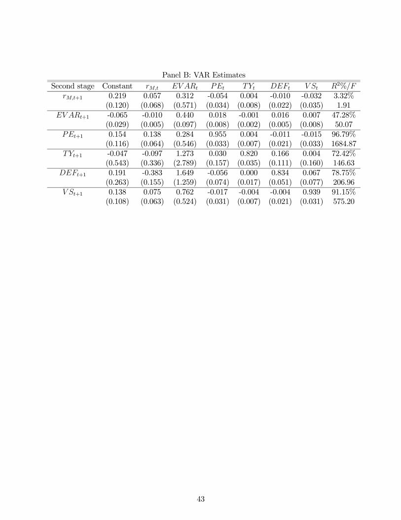
Panel B: VAR Estimates

Second stage Constant 2%/

+1 0.219 0.057 0.312 -0.054 0.004 -0.010 -0.032 3.32%

(0.120) (0.068) (0.571) (0.034) (0.008) (0.022) (0.035) 1.91

+1 -0.065 -0.010 0.440 0.018 -0.001 0.016 0.007 47.28%

(0.029) (0.005) (0.097) (0.008) (0.002) (0.005) (0.008) 50.07

+1 0.154 0.138 0.284 0.955 0.004 -0.011 -0.015 96.79%

(0.116) (0.064) (0.546) (0.033) (0.007) (0.021) (0.033) 1684.87

+1 -0.047 -0.097 1.273 0.030 0.820 0.166 0.004 72.42%

(0.543) (0.336) (2.789) (0.157) (0.035) (0.111) (0.160) 146.63

+1 0.191 -0.383 1.649 -0.056 0.000 0.834 0.067 78.75%

(0.263) (0.155) (1.259) (0.074) (0.017) (0.051) (0.077) 206.96

+1 0.138 0.075 0.762 -0.017 -0.004 -0.004 0.939 91.15%

(0.108) (0.063) (0.524) (0.031) (0.007) (0.021) (0.031) 575.20

43

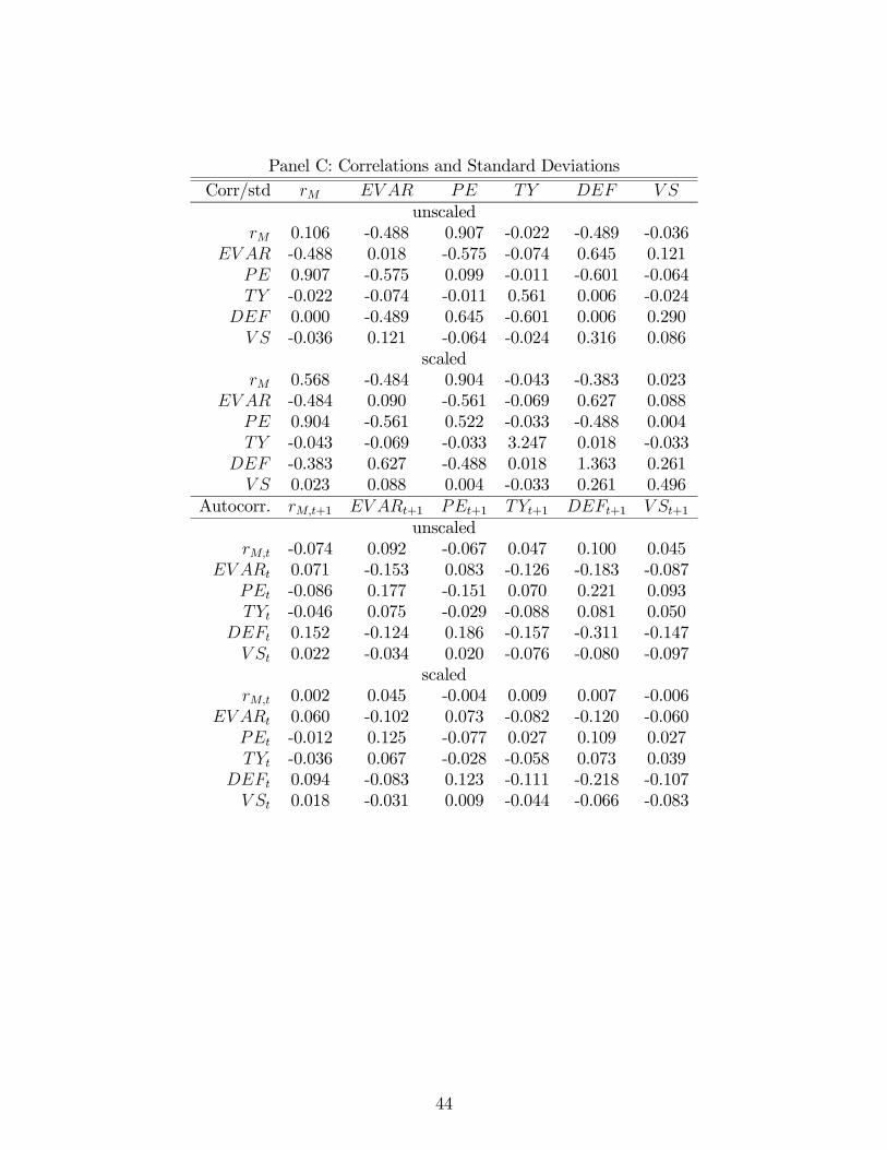
Panel C: Correlations and Standard Deviations

Corr/std

unscaled

0.106 -0.488 0.907 -0.022 -0.489 -0.036

-0.488 0.018 -0.575 -0.074 0.645 0.121

0.907 -0.575 0.099 -0.011 -0.601 -0.064

-0.022 -0.074 -0.011 0.561 0.006 -0.024

0.000 -0.489 0.645 -0.601 0.006 0.290

-0.036 0.121 -0.064 -0.024 0.316 0.086

scaled

0.568 -0.484 0.904 -0.043 -0.383 0.023

-0.484 0.090 -0.561 -0.069 0.627 0.088

0.904 -0.561 0.522 -0.033 -0.488 0.004

-0.043 -0.069 -0.033 3.247 0.018 -0.033

-0.383 0.627 -0.488 0.018 1.363 0.261

0.023 0.088 0.004 -0.033 0.261 0.496

Autocorr. +1 +1 +1 +1 +1 +1unscaled

-0.074 0.092 -0.067 0.047 0.100 0.045

0.071 -0.153 0.083 -0.126 -0.183 -0.087

-0.086 0.177 -0.151 0.070 0.221 0.093

-0.046 0.075 -0.029 -0.088 0.081 0.050

0.152 -0.124 0.186 -0.157 -0.311 -0.147

0.022 -0.034 0.020 -0.076 -0.080 -0.097

scaled

0.002 0.045 -0.004 0.009 0.007 -0.006

0.060 -0.102 0.073 -0.082 -0.120 -0.060

-0.012 0.125 -0.077 0.027 0.109 0.027

-0.036 0.067 -0.028 -0.058 0.073 0.039

0.094 -0.083 0.123 -0.111 -0.218 -0.107

0.018 -0.031 0.009 -0.044 -0.066 -0.083

44

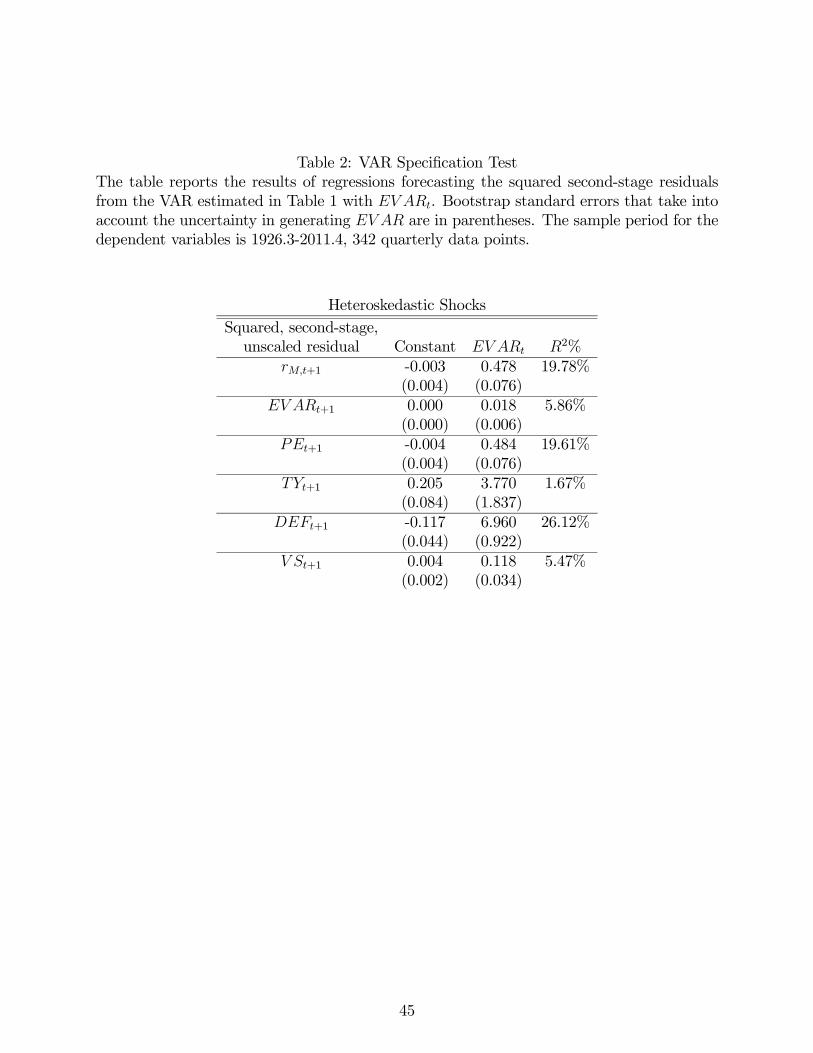
Table 2: VAR Specification Test

The table reports the results of regressions forecasting the squared second-stage residuals

from the VAR estimated in Table 1 with . Bootstrap standard errors that take into

account the uncertainty in generating are in parentheses. The sample period for the

dependent variables is 1926.3-2011.4, 342 quarterly data points.

Heteroskedastic Shocks

Squared, second-stage,

unscaled residual Constant 2%

+1 -0.003 0.478 19.78%

(0.004) (0.076)

+1 0.000 0.018 5.86%

(0.000) (0.006)

+1 -0.004 0.484 19.61%

(0.004) (0.076)

+1 0.205 3.770 1.67%

(0.084) (1.837)

+1 -0.117 6.960 26.12%

(0.044) (0.922)

+1 0.004 0.118 5.47%

(0.002) (0.034)

45

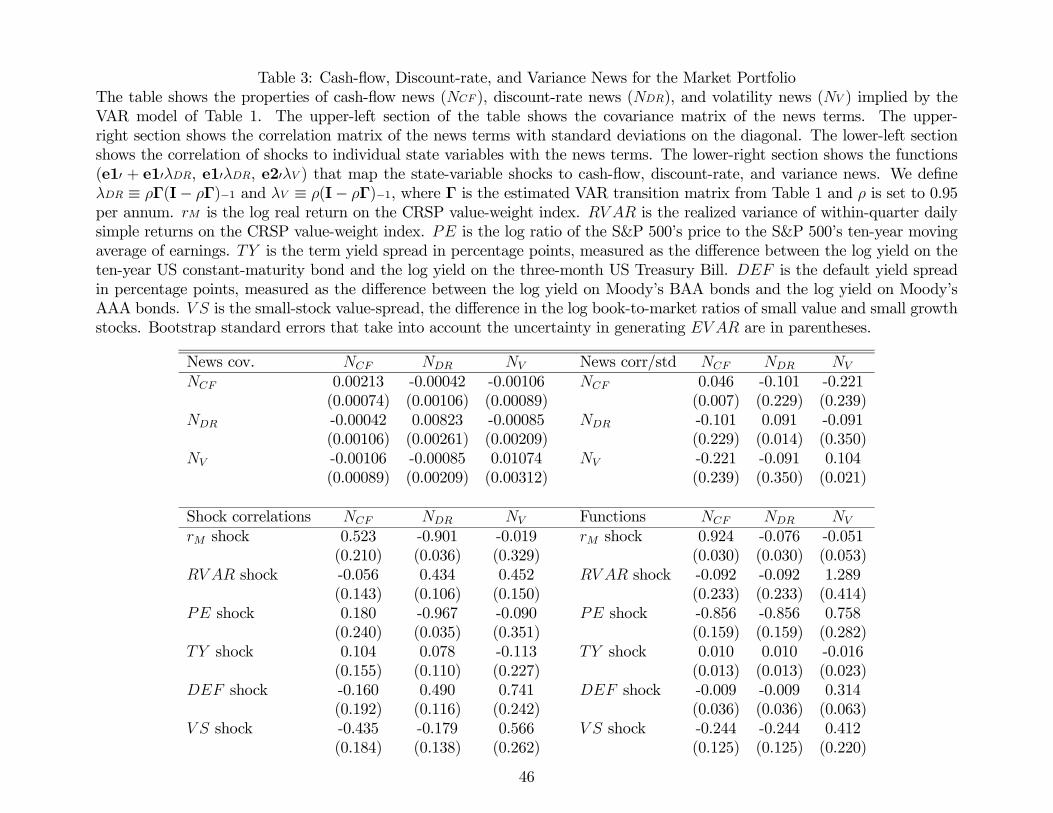
Table 3: Cash-flow, Discount-rate, and Variance News for the Market Portfolio

The table shows the properties of cash-flow news ( ), discount-rate news (), and volatility news ( ) implied by the

VAR model of Table 1. The upper-left section of the table shows the covariance matrix of the news terms. The upper-

right section shows the correlation matrix of the news terms with standard deviations on the diagonal. The lower-left section

shows the correlation of shocks to individual state variables with the news terms. The lower-right section shows the functions

(e10 + e10, e10, e20 ) that map the state-variable shocks to cash-flow, discount-rate, and variance news. We define ≡ Γ(I− Γ)−1 and ≡ (I− Γ)−1, where Γ is the estimated VAR transition matrix from Table 1 and is set to 0.95

per annum. is the log real return on the CRSP value-weight index. is the realized variance of within-quarter daily

simple returns on the CRSP value-weight index. is the log ratio of the S&P 500’s price to the S&P 500’s ten-year moving

average of earnings. is the term yield spread in percentage points, measured as the difference between the log yield on the

ten-year US constant-maturity bond and the log yield on the three-month US Treasury Bill. is the default yield spread

in percentage points, measured as the difference between the log yield on Moody’s BAA bonds and the log yield on Moody’s

AAA bonds. is the small-stock value-spread, the difference in the log book-to-market ratios of small value and small growth

stocks. Bootstrap standard errors that take into account the uncertainty in generating are in parentheses.

News cov. News corr/std

0.00213 -0.00042 -0.00106 0.046 -0.101 -0.221

(0.00074) (0.00106) (0.00089) (0.007) (0.229) (0.239)

-0.00042 0.00823 -0.00085 -0.101 0.091 -0.091

(0.00106) (0.00261) (0.00209) (0.229) (0.014) (0.350)

-0.00106 -0.00085 0.01074 -0.221 -0.091 0.104

(0.00089) (0.00209) (0.00312) (0.239) (0.350) (0.021)

Shock correlations Functions

shock 0.523 -0.901 -0.019 shock 0.924 -0.076 -0.051

(0.210) (0.036) (0.329) (0.030) (0.030) (0.053)

shock -0.056 0.434 0.452 shock -0.092 -0.092 1.289

(0.143) (0.106) (0.150) (0.233) (0.233) (0.414)

shock 0.180 -0.967 -0.090 shock -0.856 -0.856 0.758

(0.240) (0.035) (0.351) (0.159) (0.159) (0.282)

shock 0.104 0.078 -0.113 shock 0.010 0.010 -0.016

(0.155) (0.110) (0.227) (0.013) (0.013) (0.023)

shock -0.160 0.490 0.741 shock -0.009 -0.009 0.314

(0.192) (0.116) (0.242) (0.036) (0.036) (0.063)

shock -0.435 -0.179 0.566 shock -0.244 -0.244 0.412

(0.184) (0.138) (0.262) (0.125) (0.125) (0.220)

46

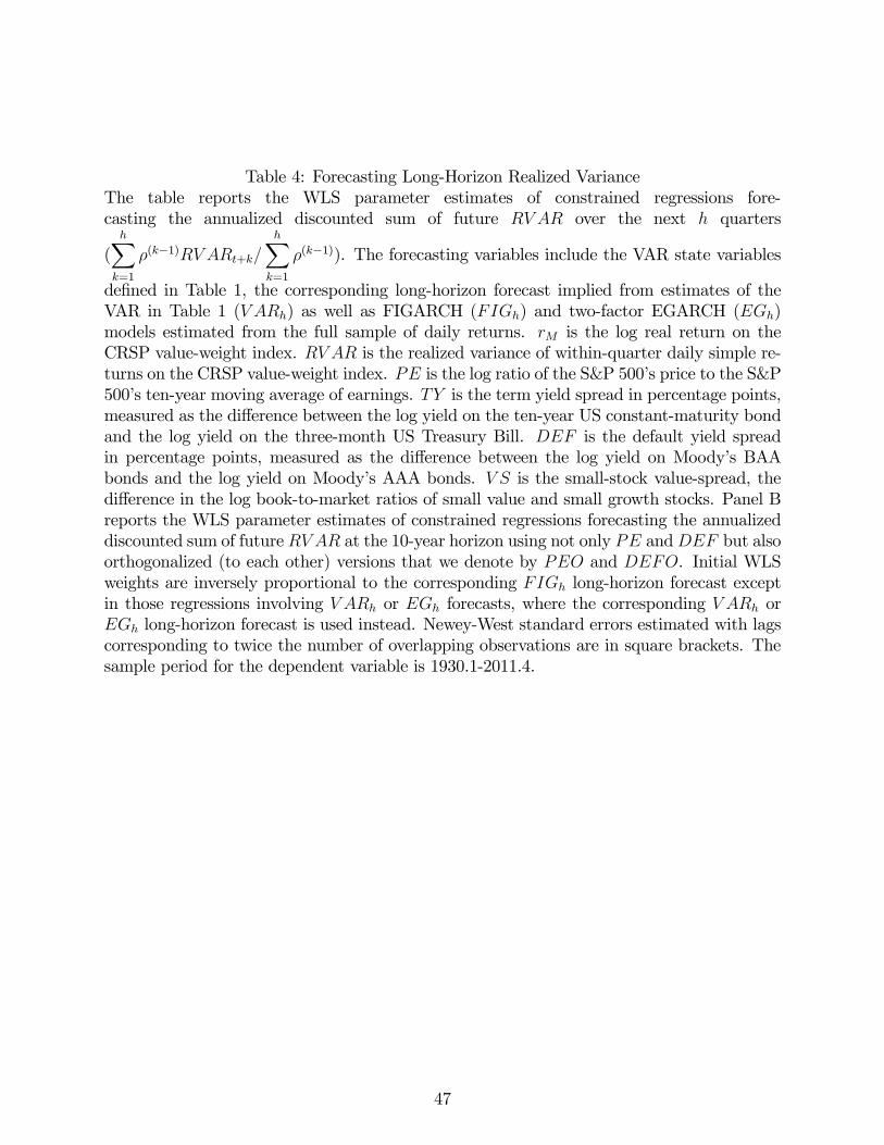
Table 4: Forecasting Long-Horizon Realized Variance

The table reports the WLS parameter estimates of constrained regressions fore-

casting the annualized discounted sum of future over the next quarters

(

X=1

(−1) +

X=1

(−1)). The forecasting variables include the VAR state variables

defined in Table 1, the corresponding long-horizon forecast implied from estimates of the

VAR in Table 1 ( ) as well as FIGARCH () and two-factor EGARCH ()

models estimated from the full sample of daily returns. is the log real return on the

CRSP value-weight index. is the realized variance of within-quarter daily simple re-

turns on the CRSP value-weight index. is the log ratio of the S&P 500’s price to the S&P

500’s ten-year moving average of earnings. is the term yield spread in percentage points,

measured as the difference between the log yield on the ten-year US constant-maturity bond

and the log yield on the three-month US Treasury Bill. is the default yield spread

in percentage points, measured as the difference between the log yield on Moody’s BAA

bonds and the log yield on Moody’s AAA bonds. is the small-stock value-spread, the

difference in the log book-to-market ratios of small value and small growth stocks. Panel B

reports the WLS parameter estimates of constrained regressions forecasting the annualized

discounted sum of future at the 10-year horizon using not only and but also

orthogonalized (to each other) versions that we denote by and . Initial WLS

weights are inversely proportional to the corresponding long-horizon forecast except

in those regressions involving or forecasts, where the corresponding or

long-horizon forecast is used instead. Newey-West standard errors estimated with lags

corresponding to twice the number of overlapping observations are in square brackets. The

sample period for the dependent variable is 1930.1-2011.4.

47

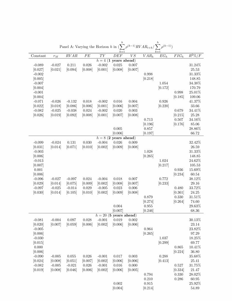
Panel A: Varying the Horizon in (

X=1

(−1) +

X=1

(−1))

Constant 2%/

= 4 (1 years ahead)

-0.089 -0.027 0.211 0.026 -0.002 0.025 0.007 31.24%

[0.027] [0.021] [0.094] [0.008] [0.001] [0.008] [0.007] 25.53

-0.002 0.998 31.33%

[0.005] [0.218] 148.85

-0.007 1.054 34.38%

[0.004] [0.172] 170.79

-0.001 0.998 25.01%

[0.004] [0.185] 109.06

-0.071 -0.026 -0.132 0.018 -0.002 0.016 0.004 0.926 41.37%

[0.022] [0.018] [0.086] [0.006] [0.001] [0.006] [0.007] [0.220] 33.66

-0.082 -0.025 -0.038 0.024 -0.002 0.020 0.003 0.679 34.41%

[0.026] [0.019] [0.092] [0.008] [0.001] [0.007] [0.008] [0.215] 25.28

0.713 0.507 34.16%

[0.196] [0.176] 85.06

0.005 0.857 28.86%

[0.006] [0.197] 66.72

= 8 (2 years ahead)

-0.099 -0.024 0.131 0.030 -0.004 0.026 0.009 32.42%

[0.031] [0.014] [0.071] [0.010] [0.002] [0.009] [0.008] 26.59

-0.003 1.028 31.33%

[0.006] [0.265] 148.85

-0.013 1.024 24.62%

[0.007] [0.217] 105.53

0.001 0.936 15.69%

[0.006] [0.234] 60.54

-0.096 -0.027 -0.097 0.024 -0.004 0.018 0.007 0.772 38.12%

[0.029] [0.014] [0.075] [0.009] [0.002] [0.008] [0.007] [0.233] 29.16

-0.097 -0.025 -0.014 0.029 -0.005 0.023 0.006 0.480 33.72%

[0.030] [0.014] [0.105] [0.010] [0.002] [0.009] [0.008] [0.361] 24.25

0.879 0.330 31.51%

[0.274] [0.264] 74.60

0.004 0.955 29.63%

[0.007] [0.246] 68.36

= 20 (5 years ahead)

-0.081 -0.004 0.097 0.028 -0.001 0.019 0.002 30.13%

[0.020] [0.007] [0.059] [0.006] [0.002] [0.006] [0.006] 23.14

-0.005 0.964 23.82%

[0.006] [0.265] 97.29

-0.030 1.037 18.25%

[0.015] [0.299] 69.77

0.000 0.865 10.41%

[0.006] [0.224] 36.80

-0.090 -0.005 0.055 0.026 -0.001 0.017 0.003 0.288 35.68%

[0.024] [0.008] [0.051] [0.007] [0.002] [0.006] [0.006] [0.413] 25.41

-0.082 -0.005 -0.021 0.026 -0.001 0.016 0.000 0.527 31.75%

[0.019] [0.008] [0.046] [0.006] [0.002] [0.006] [0.005] [0.334] 21.47

0.794 0.330 28.02%

0.210 0.286 60.95

0.002 0.915 25.92%

[0.004] [0.214] 54.89

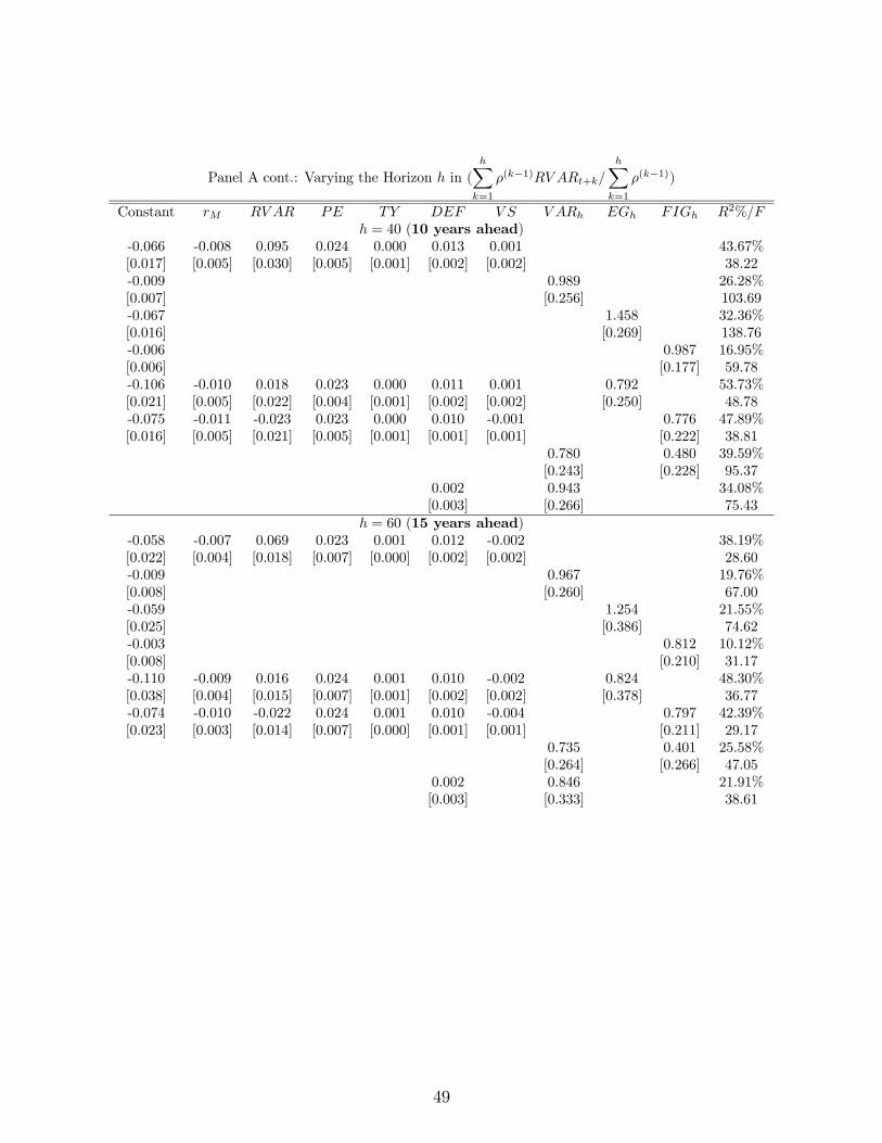
Panel A cont.: Varying the Horizon in (

X=1

(−1) +

X=1

(−1))

Constant 2%/

= 40 (10 years ahead)

-0.066 -0.008 0.095 0.024 0.000 0.013 0.001 43.67%

[0.017] [0.005] [0.030] [0.005] [0.001] [0.002] [0.002] 38.22

-0.009 0.989 26.28%

[0.007] [0.256] 103.69

-0.067 1.458 32.36%

[0.016] [0.269] 138.76

-0.006 0.987 16.95%

[0.006] [0.177] 59.78

-0.106 -0.010 0.018 0.023 0.000 0.011 0.001 0.792 53.73%

[0.021] [0.005] [0.022] [0.004] [0.001] [0.002] [0.002] [0.250] 48.78

-0.075 -0.011 -0.023 0.023 0.000 0.010 -0.001 0.776 47.89%

[0.016] [0.005] [0.021] [0.005] [0.001] [0.001] [0.001] [0.222] 38.81

0.780 0.480 39.59%

[0.243] [0.228] 95.37

0.002 0.943 34.08%

[0.003] [0.266] 75.43

= 60 (15 years ahead)

-0.058 -0.007 0.069 0.023 0.001 0.012 -0.002 38.19%

[0.022] [0.004] [0.018] [0.007] [0.000] [0.002] [0.002] 28.60

-0.009 0.967 19.76%

[0.008] [0.260] 67.00

-0.059 1.254 21.55%

[0.025] [0.386] 74.62

-0.003 0.812 10.12%

[0.008] [0.210] 31.17

-0.110 -0.009 0.016 0.024 0.001 0.010 -0.002 0.824 48.30%

[0.038] [0.004] [0.015] [0.007] [0.001] [0.002] [0.002] [0.378] 36.77

-0.074 -0.010 -0.022 0.024 0.001 0.010 -0.004 0.797 42.39%

[0.023] [0.003] [0.014] [0.007] [0.000] [0.001] [0.001] [0.211] 29.17

0.735 0.401 25.58%

[0.264] [0.266] 47.05

0.002 0.846 21.91%

[0.003] [0.333] 38.61

49

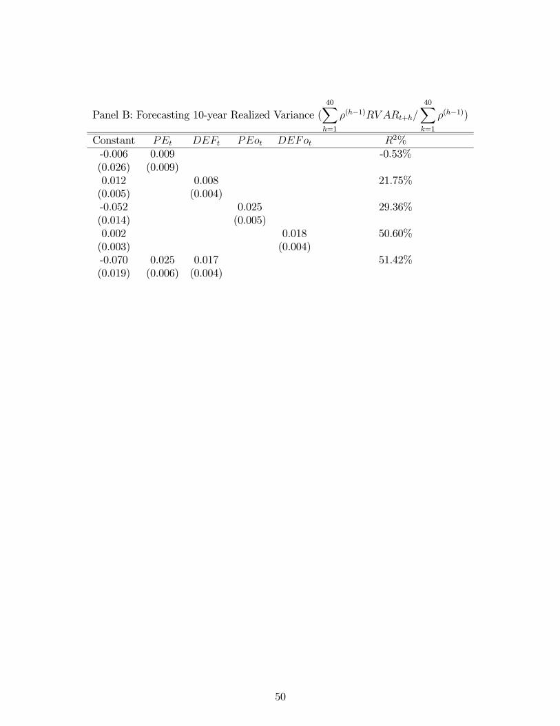
Panel B: Forecasting 10-year Realized Variance (

40X=1

(−1) +

40X=1

(−1))

Constant 2%

-0.006 0.009 -0.53%

(0.026) (0.009)

0.012 0.008 21.75%

(0.005) (0.004)

-0.052 0.025 29.36%

(0.014) (0.005)

0.002 0.018 50.60%

(0.003) (0.004)

-0.070 0.025 0.017 51.42%

(0.019) (0.006) (0.004)

50

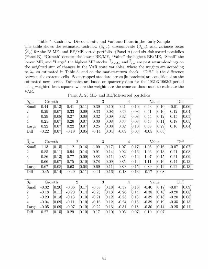
Table 5: Cash-flow, Discount-rate, and Variance Betas in the Early Sample

The table shows the estimated cash-flow (b ), discount-rate (b), and variance betas

(b ) for the 25 ME- and BE/ME-sorted portfolios (Panel A) and six risk-sorted portfolios(Panel B). “Growth” denotes the lowest BE/ME, “Value” the highest BE/ME, “Small” the

lowest ME, and "Large" the highest ME stocks. b∆ and b are past return-loadings on

the weighted sum of changes in the VAR state variables, where the weights are according

to as estimated in Table 3, and on the market-return shock. “Diff.” is the difference

between the extreme cells. Bootstrapped standard errors [in brackets] are conditional on the

estimated news series. Estimates are based on quarterly data for the 1931:3-1963:2 period

using weighted least squares where the weights are the same as those used to estimate the

VAR.Panel A: 25 ME- and BE/ME-sorted portfoliosb Growth 2 3 4 Value Diff

Small 0.44 [0.13] 0.41 [0.11] 0.39 [0.10] 0.41 [0.10] 0.43 [0.10] -0.01 [0.06]

2 0.29 [0.07] 0.33 [0.09] 0.33 [0.08] 0.36 [0.08] 0.41 [0.10] 0.12 [0.04]

3 0.29 [0.08] 0.27 [0.08] 0.32 [0.09] 0.32 [0.08] 0.44 [0.12] 0.15 [0.05]

4 0.25 [0.07] 0.26 [0.07] 0.30 [0.08] 0.33 [0.08] 0.43 [0.11] 0.18 [0.05]

Large 0.22 [0.07] 0.22 [0.07] 0.25 [0.08] 0.32 [0.10] 0.38 [0.29] 0.16 [0.04]

Diff -0.22 [0.07] -0.19 [0.05] -0.14 [0.04] -0.09 [0.03] -0.05 [0.03]

b Growth 2 3 4 Value Diff

Small 1.13 [0.15] 1.12 [0.16] 1.09 [0.17] 1.07 [0.17] 1.05 [0.16] -0.07 [0.07]

2 0.85 [0.11] 0.94 [0.14] 0.91 [0.14] 0.92 [0.16] 1.06 [0.13] 0.21 [0.08]

3 0.86 [0.13] 0.77 [0.09] 0.88 [0.11] 0.86 [0.12] 1.07 [0.15] 0.21 [0.09]

4 0.66 [0.07] 0.75 [0.10] 0.78 [0.09] 0.85 [0.14] 1.11 [0.16] 0.44 [0.13]

Large 0.67 [0.08] 0.63 [0.08] 0.69 [0.11] 0.89 [0.15] 0.89 [0.12] 0.22 [0.13]

Diff -0.45 [0.14] -0.49 [0.11] -0.41 [0.16] -0.18 [0.13] -0.17 [0.08]

b Growth 2 3 4 Value Diff

Small -0.32 [0.20] -0.36 [0.17] -0.38 [0.18] -0.37 [0.16] -0.40 [0.17] -0.07 [0.09]

2 -0.18 [0.11] -0.20 [0.14] -0.25 [0.13] -0.26 [0.14] -0.38 [0.18] -0.20 [0.08]

3 -0.20 [0.13] -0.13 [0.10] -0.21 [0.12] -0.23 [0.13] -0.39 [0.18] -0.20 [0.08]

4 -0.04 [0.09] -0.11 [0.10] -0.16 [0.12] -0.24 [0.15] -0.39 [0.19] -0.35 [0.13]

Large -0.05 [0.09] -0.07 [0.10] -0.22 [0.16] -0.31 [0.18] -0.30 [0.14] -0.25 [0.11]

Diff 0.27 [0.15] 0.29 [0.10] 0.17 [0.10] 0.05 [0.07] 0.10 [0.07]

51

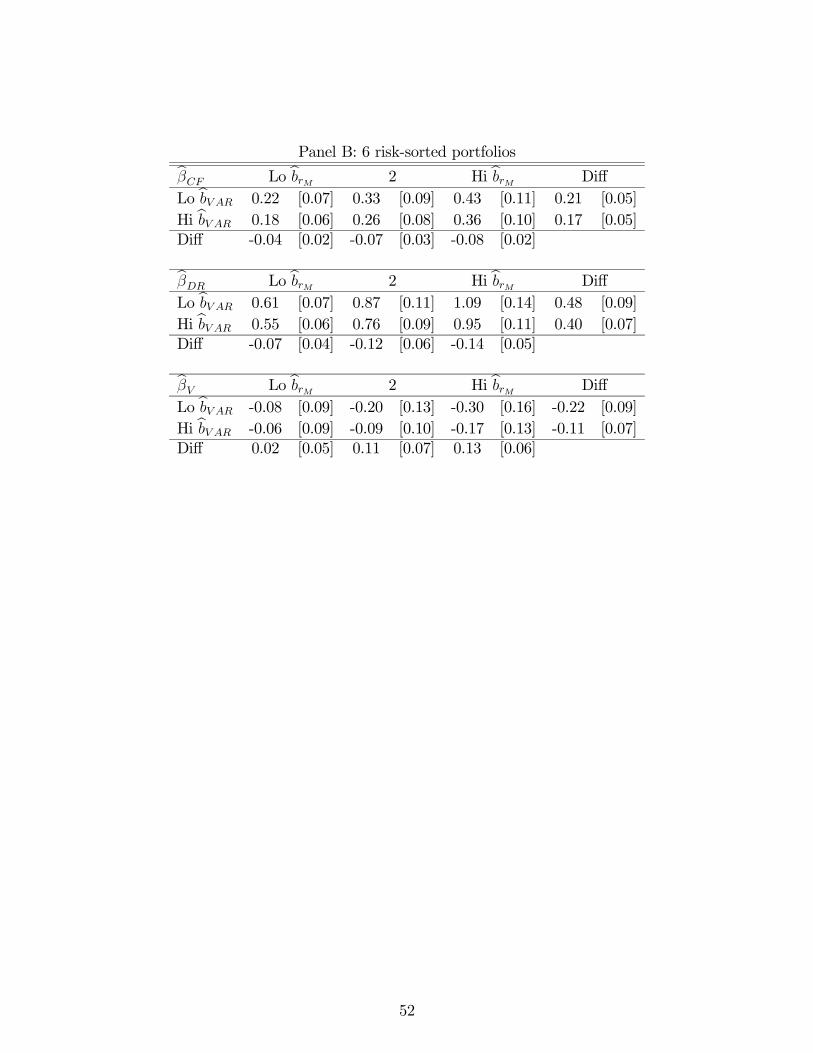
Panel B: 6 risk-sorted portfoliosb Lo b 2 Hi b Diff

Lo b 0.22 [0.07] 0.33 [0.09] 0.43 [0.11] 0.21 [0.05]

Hi b 0.18 [0.06] 0.26 [0.08] 0.36 [0.10] 0.17 [0.05]

Diff -0.04 [0.02] -0.07 [0.03] -0.08 [0.02]

b Lo b 2 Hi b Diff

Lo b 0.61 [0.07] 0.87 [0.11] 1.09 [0.14] 0.48 [0.09]

Hi b 0.55 [0.06] 0.76 [0.09] 0.95 [0.11] 0.40 [0.07]

Diff -0.07 [0.04] -0.12 [0.06] -0.14 [0.05]

b Lo b 2 Hi b Diff

Lo b -0.08 [0.09] -0.20 [0.13] -0.30 [0.16] -0.22 [0.09]

Hi b -0.06 [0.09] -0.09 [0.10] -0.17 [0.13] -0.11 [0.07]

Diff 0.02 [0.05] 0.11 [0.07] 0.13 [0.06]

52

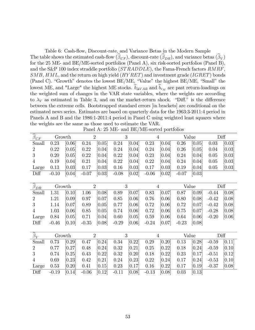
Table 6: Cash-flow, Discount-rate, and Variance Betas in the Modern Sample

The table shows the estimated cash-flow (b ), discount-rate (b), and variance betas (b )

for the 25 ME- and BE/ME-sorted portfolios (Panel A), six risk-sorted portfolios (Panel B),

and the S&P 100 index straddle portfolio (), the Fama-French factors ,

,, and the return on high yield ( ) and investment grade ( ) bonds

(Panel C). “Growth” denotes the lowest BE/ME, “Value” the highest BE/ME, “Small” the

lowest ME, and "Large" the highest ME stocks. b∆ and b are past return-loadings on

the weighted sum of changes in the VAR state variables, where the weights are according

to as estimated in Table 3, and on the market-return shock. “Diff.” is the difference

between the extreme cells. Bootstrapped standard errors [in brackets] are conditional on the

estimated news series. Estimates are based on quarterly data for the 1963:3-2011:4 period in

Panels A and B and the 1986:1-2011:4 period in Panel C using weighted least squares where

the weights are the same as those used to estimate the VAR.Panel A: 25 ME- and BE/ME-sorted portfoliosb Growth 2 3 4 Value Diff

Small 0.23 [0.06] 0.24 [0.05] 0.24 [0.04] 0.23 [0.04] 0.26 [0.05] 0.03 [0.03]

2 0.22 [0.05] 0.22 [0.04] 0.24 [0.04] 0.24 [0.04] 0.26 [0.05] 0.04 [0.03]

3 0.20 [0.05] 0.22 [0.04] 0.22 [0.04] 0.23 [0.04] 0.24 [0.04] 0.05 [0.03]

4 0.19 [0.04] 0.21 [0.04] 0.22 [0.04] 0.22 [0.04] 0.24 [0.04] 0.05 [0.03]

Large 0.13 [0.03] 0.17 [0.03] 0.16 [0.03] 0.17 [0.03] 0.19 [0.04] 0.05 [0.03]

Diff -0.10 [0.04] -0.07 [0.03] -0.08 [0.02] -0.06 [0.02] -0.07 [0.03]

b Growth 2 3 4 Value Diff

Small 1.31 [0.10] 1.06 [0.08] 0.89 [0.07] 0.83 [0.07] 0.87 [0.09] -0.44 [0.08]

2 1.21 [0.09] 0.97 [0.07] 0.85 [0.06] 0.76 [0.06] 0.80 [0.08] -0.42 [0.08]

3 1.14 [0.07] 0.89 [0.05] 0.77 [0.06] 0.72 [0.06] 0.72 [0.07] -0.42 [0.08]

4 1.03 [0.06] 0.85 [0.05] 0.74 [0.06] 0.72 [0.06] 0.75 [0.07] -0.28 [0.08]

Large 0.84 [0.05] 0.71 [0.04] 0.60 [0.05] 0.59 [0.06] 0.64 [0.06] -0.20 [0.06]

Diff -0.46 [0.10] -0.35 [0.08] -0.29 [0.06] -0.24 [0.07] -0.23 [0.08]

b Growth 2 3 4 Value Diff

Small 0.73 [0.29] 0.47 [0.24] 0.34 [0.22] 0.29 [0.20] 0.13 [0.28] -0.59 [0.11]

2 0.77 [0.27] 0.48 [0.24] 0.32 [0.21] 0.25 [0.22] 0.18 [0.24] -0.59 [0.10]

3 0.74 [0.25] 0.43 [0.22] 0.32 [0.20] 0.18 [0.22] 0.23 [0.17] -0.51 [0.12]

4 0.69 [0.23] 0.42 [0.21] 0.24 [0.23] 0.22 [0.24] 0.17 [0.24] -0.53 [0.10]

Large 0.53 [0.20] 0.41 [0.15] 0.23 [0.17] 0.16 [0.22] 0.17 [0.19] -0.37 [0.08]

Diff -0.19 [0.14] -0.06 [0.12] -0.11 [0.08] -0.13 [0.08] 0.03 [0.13]

53

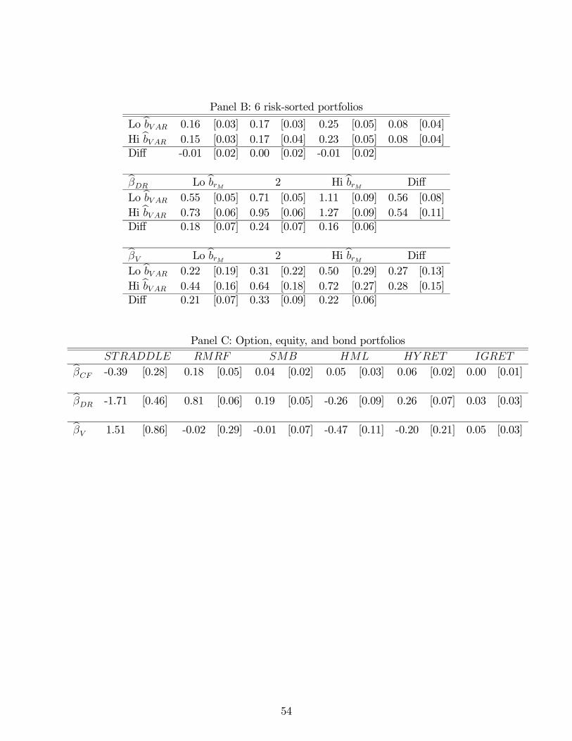
Panel B: 6 risk-sorted portfolios

Lo b 0.16 [0.03] 0.17 [0.03] 0.25 [0.05] 0.08 [0.04]

Hi b 0.15 [0.03] 0.17 [0.04] 0.23 [0.05] 0.08 [0.04]

Diff -0.01 [0.02] 0.00 [0.02] -0.01 [0.02]

b Lo b 2 Hi b Diff

Lo b 0.55 [0.05] 0.71 [0.05] 1.11 [0.09] 0.56 [0.08]

Hi b 0.73 [0.06] 0.95 [0.06] 1.27 [0.09] 0.54 [0.11]

Diff 0.18 [0.07] 0.24 [0.07] 0.16 [0.06]

b Lo b 2 Hi b Diff

Lo b 0.22 [0.19] 0.31 [0.22] 0.50 [0.29] 0.27 [0.13]

Hi b 0.44 [0.16] 0.64 [0.18] 0.72 [0.27] 0.28 [0.15]

Diff 0.21 [0.07] 0.33 [0.09] 0.22 [0.06]

Panel C: Option, equity, and bond portfolios

b -0.39 [0.28] 0.18 [0.05] 0.04 [0.02] 0.05 [0.03] 0.06 [0.02] 0.00 [0.01]

b -1.71 [0.46] 0.81 [0.06] 0.19 [0.05] -0.26 [0.09] 0.26 [0.07] 0.03 [0.03]

b 1.51 [0.86] -0.02 [0.29] -0.01 [0.07] -0.47 [0.11] -0.20 [0.21] 0.05 [0.03]

54

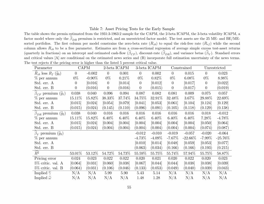
Table 7: Asset Pricing Tests for the Early Sample

The table shows the premia estimated from the 1931:3-1963:2 sample for the CAPM, the 2-beta ICAPM, the 3-beta volatility ICAPM, a

factor model where only the b premium is restricted, and an unrestricted factor model. The test assets are the 25 ME- and BE/ME-

sorted portfolios. The first column per model constrains the zero-beta rate () to equal the risk-free rate ( ) while the second

column allows to be a free parameter. Estimates are from a cross-sectional regression of average simple excess test-asset returns

(quarterly in fractions) on an intercept and estimated cash-flow (b ), discount-rate (b), and variance betas (b ). Standard errors

and critical values [A] are conditional on the estimated news series and (B) incorporate full estimation uncertainty of the news terms.

The test rejects if the pricing error is higher than the listed 5 percent critical value.

Parameter CAPM 2-beta ICAPM 3-beta ICAPM Constrained Unrestrictedb less (b0) 0 -0.002 0 0.001 0 0.002 0 0.015 0 0.023

% per annum 0% -0.90% 0% 0.21% 0% 0.82% 0% 6.08% 0% 8.98%

Std. err. A 0 [0.016] 0 [0.014] 0 [0.012] 0 [0.017] 0 [0.022]

Std. err. B 0 (0.016) 0 (0.016) 0 (0.015) 0 (0.017) 0 (0.019)b premium (b1) 0.038 0.040 0.096 0.094 0.087 0.082 0.081 0.009 0.075 0.057

% per annum 15.11% 15.82% 38.33% 37.74% 34.75% 32.91% 32.48% 3.67% 29.88% 22.69%

Std. err. A [0.015] [0.024] [0.054] [0.079] [0.041] [0.053] [0.061] [0.104] [0.124] [0.129]

Std. err. B (0.015) (0.024) (0.145) (0.110) (0.096) (0.091) (0.105) (0.118) (0.129) (0.138)b premium (b2) 0.038 0.040 0.016 0.016 0.016 0.016 0.016 0.016 0.018 -0.012

% per annum 15.11% 15.82% 6.40% 6.40% 6.40% 6.40% 6.40% 6.40% 7.28% -4.78%

Std. err. A [0.015] [0.024] [0.004] [0.004] [0.004] [0.004] [0.004] [0.004] [0.050] [0.064]

Std. err. B (0.015) (0.024) (0.004) (0.004) (0.004) (0.004) (0.004) (0.004) (0.074) (0.087)b premium (b3) -0.012 -0.010 -0.019 -0.057 -0.020 -0.064

% per annum -4.73% -4.09% -7.67% -22.66% -7.99% -25.76%

Std. err. A [0.010] [0.014] [0.048] [0.059] [0.053] [0.077]

Std. err. B (0.063) (0.034) (0.166) (0.166) (0.193) (0.215)c2 53.01% 53.12% 54.72% 54.73% 55.59% 55.75% 55.74% 57.94% 55.75% 58.87%

Pricing error 0.024 0.023 0.022 0.022 0.020 0.021 0.020 0.022 0.020 0.023

5% critic. val. A [0.064] [0.031] [0.060] [0.038] [0.067] [0.044] [0.044] [0.038] [0.038] [0.039]

5% critic. val. B (0.064) (0.031) (0.106) (0.046) (0.133) (0.053) (0.049) (0.040) (0.039) (0.043)

Implied b N/A N/A 5.99 5.90 5.43 5.14 N/A N/A N/A N/A

Implied b N/A N/A N/A N/A 1.48 1.28 N/A N/A N/A N/A

55

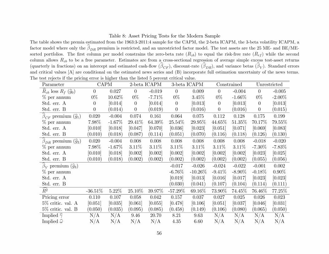
Table 8: Asset Pricing Tests for the Modern Sample

The table shows the premia estimated from the 1963:3-2011:4 sample for the CAPM, the 2-beta ICAPM, the 3-beta volatility ICAPM, a

factor model where only the b premium is restricted, and an unrestricted factor model. The test assets are the 25 ME- and BE/ME-

sorted portfolios. The first column per model constrains the zero-beta rate () to equal the risk-free rate ( ) while the second

column allows to be a free parameter. Estimates are from a cross-sectional regression of average simple excess test-asset returns

(quarterly in fractions) on an intercept and estimated cash-flow (b ), discount-rate (b), and variance betas (b ). Standard errors

and critical values [A] are conditional on the estimated news series and (B) incorporate full estimation uncertainty of the news terms.

The test rejects if the pricing error is higher than the listed 5 percent critical value.

Parameter CAPM 2-beta ICAPM 3-beta ICAPM Constrained Unrestrictedb less (b0) 0 0.027 0 -0.019 0 0.009 0 -0.004 0 -0.005

% per annum 0% 10.62% 0% -7.71% 0% 3.45% 0% -1.66% 0% -2.00%

Std. err. A 0 [0.014] 0 [0.014] 0 [0.013] 0 [0.013] 0 [0.013]

Std. err. B 0 (0.014) 0 (0.019) 0 (0.016) 0 (0.016) 0 (0.015)b premium (b1) 0.020 -0.004 0.074 0.161 0.064 0.075 0.112 0.128 0.175 0.199

% per annum 7.98% -1.67% 29.41% 64.39% 25.54% 29.95% 44.65% 51.35% 70.17% 79.55%

Std. err. A [0.010] [0.018] [0.047] [0.070] [0.036] [0.023] [0.051] [0.071] [0.069] [0.083]

Std. err. B (0.010) (0.018) (0.087) (0.114) (0.051) (0.070) (0.116) (0.118) (0.126) (0.130)b premium (b2) 0.020 -0.004 0.008 0.008 0.008 0.008 0.008 0.008 -0.018 -0.020

% per annum 7.98% -1.67% 3.11% 3.11% 3.11% 3.11% 3.11% 3.11% -7.30% -7.83%

Std. err. A [0.010] [0.018] [0.002] [0.002] [0.002] [0.002] [0.002] [0.002] [0.023] [0.025]

Std. err. B (0.010) (0.018) (0.002) (0.002) (0.002) (0.002) (0.002) (0.002) (0.055) (0.056)b premium (b3) -0.017 -0.026 -0.024 -0.022 -0.001 0.002

% per annum -6.76% -10.26% -9.41% -8.90% -0.18% 0.90%

Std. err. A [0.019] [0.013] [0.016] [0.017] [0.023] [0.023]

Std. err. B (0.030) (0.041) (0.107) (0.104) (0.114) (0.111)c2 -36.51% 5.22% 25.10% 39.97% -57.29% 69.16% 73.90% 74.45% 76.46% 77.25%

Pricing error 0.110 0.107 0.058 0.042 0.157 0.037 0.027 0.025 0.026 0.023

5% critic. val. A [0.051] [0.035] [0.061] [0.055] [0.478] [0.106] [0.051] [0.037] [0.046] [0.031]

5% critic. val. B (0.050) (0.035) (0.095) (0.085) (0.458) (0.149) (0.106) (0.080) (0.065) (0.050)

Implied b N/A N/A 9.46 20.70 8.21 9.63 N/A N/A N/A N/A

Implied b N/A N/A N/A N/A 4.35 6.60 N/A N/A N/A N/A

56

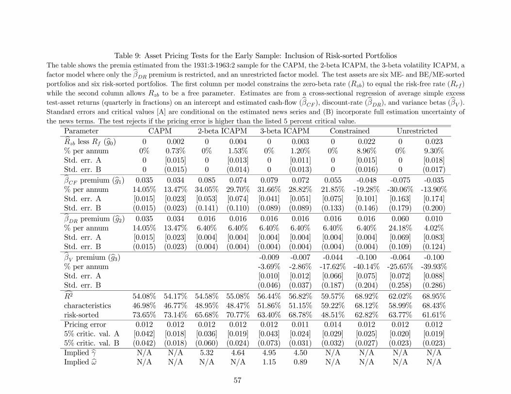
Table 9: Asset Pricing Tests for the Early Sample: Inclusion of Risk-sorted Portfolios

The table shows the premia estimated from the 1931:3-1963:2 sample for the CAPM, the 2-beta ICAPM, the 3-beta volatility ICAPM, a

factor model where only the b premium is restricted, and an unrestricted factor model. The test assets are six ME- and BE/ME-sorted

portfolios and six risk-sorted portfolios. The first column per model constrains the zero-beta rate () to equal the risk-free rate ( )

while the second column allows to be a free parameter. Estimates are from a cross-sectional regression of average simple excess

test-asset returns (quarterly in fractions) on an intercept and estimated cash-flow (b ), discount-rate (b), and variance betas (b ).

Standard errors and critical values [A] are conditional on the estimated news series and (B) incorporate full estimation uncertainty of

the news terms. The test rejects if the pricing error is higher than the listed 5 percent critical value.

Parameter CAPM 2-beta ICAPM 3-beta ICAPM Constrained Unrestrictedb less (b0) 0 0.002 0 0.004 0 0.003 0 0.022 0 0.023

% per annum 0% 0.73% 0% 1.53% 0% 1.20% 0% 8.96% 0% 9.30%

Std. err. A 0 [0.015] 0 [0.013] 0 [0.011] 0 [0.015] 0 [0.018]

Std. err. B 0 (0.015) 0 (0.014) 0 (0.013) 0 (0.016) 0 (0.017)b premium (b1) 0.035 0.034 0.085 0.074 0.079 0.072 0.055 -0.048 -0.075 -0.035

% per annum 14.05% 13.47% 34.05% 29.70% 31.66% 28.82% 21.85% -19.28% -30.06% -13.90%

Std. err. A [0.015] [0.023] [0.053] [0.074] [0.041] [0.051] [0.075] [0.101] [0.163] [0.174]

Std. err. B (0.015) (0.023) (0.141) (0.110) (0.089) (0.089) (0.133) (0.146) (0.179) (0.200)b premium (b2) 0.035 0.034 0.016 0.016 0.016 0.016 0.016 0.016 0.060 0.010

% per annum 14.05% 13.47% 6.40% 6.40% 6.40% 6.40% 6.40% 6.40% 24.18% 4.02%

Std. err. A [0.015] [0.023] [0.004] [0.004] [0.004] [0.004] [0.004] [0.004] [0.069] [0.083]

Std. err. B (0.015) (0.023) (0.004) (0.004) (0.004) (0.004) (0.004) (0.004) (0.109) (0.124)b premium (b3) -0.009 -0.007 -0.044 -0.100 -0.064 -0.100

% per annum -3.69% -2.86% -17.62% -40.14% -25.65% -39.93%

Std. err. A [0.010] [0.012] [0.066] [0.075] [0.072] [0.088]

Std. err. B (0.046) (0.037) (0.187) (0.204) (0.258) (0.286)c2 54.08% 54.17% 54.58% 55.08% 56.44% 56.82% 59.57% 68.92% 62.02% 68.95%

characteristics 46.98% 46.77% 48.95% 48.47% 51.86% 51.15% 59.22% 68.12% 58.99% 68.43%

risk-sorted 73.65% 73.14% 65.68% 70.77% 63.40% 68.78% 48.51% 62.82% 63.77% 61.61%

Pricing error 0.012 0.012 0.012 0.012 0.012 0.011 0.014 0.012 0.012 0.012

5% critic. val. A [0.042] [0.018] [0.036] [0.019] [0.043] [0.024] [0.029] [0.025] [0.020] [0.019]

5% critic. val. B (0.042) (0.018) (0.060) (0.024) (0.073) (0.031) (0.032) (0.027) (0.023) (0.023)

Implied b N/A N/A 5.32 4.64 4.95 4.50 N/A N/A N/A N/A

Implied b N/A N/A N/A N/A 1.15 0.89 N/A N/A N/A N/A

57

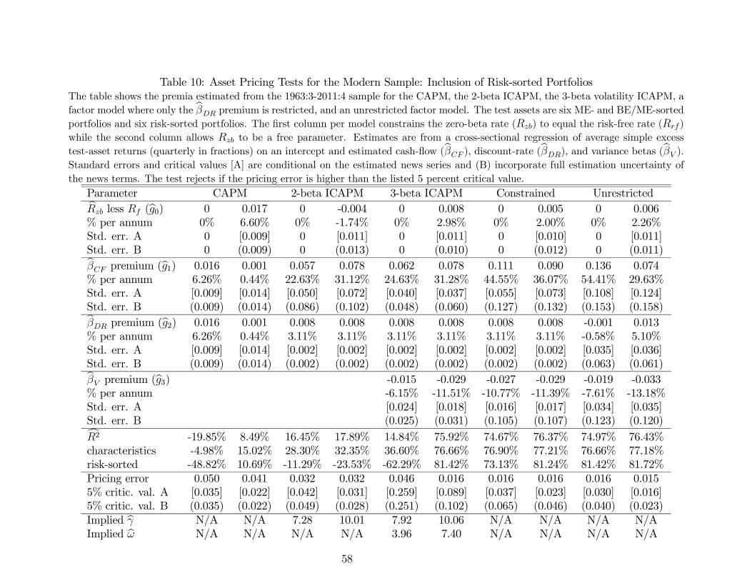
Table 10: Asset Pricing Tests for the Modern Sample: Inclusion of Risk-sorted Portfolios

The table shows the premia estimated from the 1963:3-2011:4 sample for the CAPM, the 2-beta ICAPM, the 3-beta volatility ICAPM, a

factor model where only the b premium is restricted, and an unrestricted factor model. The test assets are six ME- and BE/ME-sorted

portfolios and six risk-sorted portfolios. The first column per model constrains the zero-beta rate () to equal the risk-free rate ( )

while the second column allows to be a free parameter. Estimates are from a cross-sectional regression of average simple excess

test-asset returns (quarterly in fractions) on an intercept and estimated cash-flow (b ), discount-rate (b), and variance betas (b ).

Standard errors and critical values [A] are conditional on the estimated news series and (B) incorporate full estimation uncertainty of

the news terms. The test rejects if the pricing error is higher than the listed 5 percent critical value.

Parameter CAPM 2-beta ICAPM 3-beta ICAPM Constrained Unrestrictedb less (b0) 0 0.017 0 -0.004 0 0.008 0 0.005 0 0.006

% per annum 0% 6.60% 0% -1.74% 0% 2.98% 0% 2.00% 0% 2.26%

Std. err. A 0 [0.009] 0 [0.011] 0 [0.011] 0 [0.010] 0 [0.011]

Std. err. B 0 (0.009) 0 (0.013) 0 (0.010) 0 (0.012) 0 (0.011)b premium (b1) 0.016 0.001 0.057 0.078 0.062 0.078 0.111 0.090 0.136 0.074

% per annum 6.26% 0.44% 22.63% 31.12% 24.63% 31.28% 44.55% 36.07% 54.41% 29.63%

Std. err. A [0.009] [0.014] [0.050] [0.072] [0.040] [0.037] [0.055] [0.073] [0.108] [0.124]

Std. err. B (0.009) (0.014) (0.086) (0.102) (0.048) (0.060) (0.127) (0.132) (0.153) (0.158)b premium (b2) 0.016 0.001 0.008 0.008 0.008 0.008 0.008 0.008 -0.001 0.013

% per annum 6.26% 0.44% 3.11% 3.11% 3.11% 3.11% 3.11% 3.11% -0.58% 5.10%

Std. err. A [0.009] [0.014] [0.002] [0.002] [0.002] [0.002] [0.002] [0.002] [0.035] [0.036]

Std. err. B (0.009) (0.014) (0.002) (0.002) (0.002) (0.002) (0.002) (0.002) (0.063) (0.061)b premium (b3) -0.015 -0.029 -0.027 -0.029 -0.019 -0.033

% per annum -6.15% -11.51% -10.77% -11.39% -7.61% -13.18%

Std. err. A [0.024] [0.018] [0.016] [0.017] [0.034] [0.035]

Std. err. B (0.025) (0.031) (0.105) (0.107) (0.123) (0.120)c2 -19.85% 8.49% 16.45% 17.89% 14.84% 75.92% 74.67% 76.37% 74.97% 76.43%

characteristics -4.98% 15.02% 28.30% 32.35% 36.60% 76.66% 76.90% 77.21% 76.66% 77.18%

risk-sorted -48.82% 10.69% -11.29% -23.53% -62.29% 81.42% 73.13% 81.24% 81.42% 81.72%

Pricing error 0.050 0.041 0.032 0.032 0.046 0.016 0.016 0.016 0.016 0.015

5% critic. val. A [0.035] [0.022] [0.042] [0.031] [0.259] [0.089] [0.037] [0.023] [0.030] [0.016]

5% critic. val. B (0.035) (0.022) (0.049) (0.028) (0.251) (0.102) (0.065) (0.046) (0.040) (0.023)

Implied b N/A N/A 7.28 10.01 7.92 10.06 N/A N/A N/A N/A

Implied b N/A N/A N/A N/A 3.96 7.40 N/A N/A N/A N/A

58

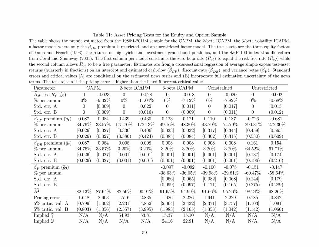
Table 11: Asset Pricing Tests for the Equity and Option Sample

The table shows the premia estimated from the 1986:1-2011:4 sample for the CAPM, the 2-beta ICAPM, the 3-beta volatility ICAPM,

a factor model where only the b premium is restricted, and an unrestricted factor model. The test assets are the three equity factors

of Fama and French (1993), the returns on high yield and investment grade bond portfolios, and the S&P 100 index straddle return

from Coval and Shumway (2001). The first column per model constrains the zero-beta rate () to equal the risk-free rate ( ) while

the second column allows to be a free parameter. Estimates are from a cross-sectional regression of average simple excess test-asset

returns (quarterly in fractions) on an intercept and estimated cash-flow (b ), discount-rate (b), and variance betas (b ). Standard

errors and critical values [A] are conditional on the estimated news series and (B) incorporate full estimation uncertainty of the news

terms. The test rejects if the pricing error is higher than the listed 5 percent critical value.

Parameter CAPM 2-beta ICAPM 3-beta ICAPM Constrained Unrestrictedb less (b0) 0 -0.023 0 -0.028 0 -0.018 0 -0.020 0 -0.002

% per annum 0% -9.02% 0% -11.04% 0% -7.12% 0% -7.82% 0% -0.68%

Std. err. A 0 [0.009] 0 [0.022] 0 [0.011] 0 [0.017] 0 [0.013]

Std. err. B 0 (0.009) 0 (0.016) 0 (0.009) 0 (0.011) 0 (0.012)b premium (b1) 0.087 0.084 0.439 0.430 0.123 0.121 0.110 0.187 -0.726 -0.681

% per annum 34.76% 33.57% 175.70% 172.13% 49.16% 48.30% 43.79% 74.79% -290.31% -272.30%

Std. err. A [0.026] [0.027] [0.330] [0.406] [0.033] [0.032] [0.317] [0.344] [0.459] [0.565]

Std. err. B (0.026) (0.027) (0.386) (0.424) (0.085) (0.084) (0.302) (0.315) (0.530) (0.609)b premium (b2) 0.087 0.084 0.008 0.008 0.008 0.008 0.008 0.008 0.161 0.154

% per annum 34.76% 33.57% 3.20% 3.20% 3.20% 3.20% 3.20% 3.20% 64.52% 61.71%

Std. err. A [0.026] [0.027] [0.001] [0.001] [0.001] [0.001] [0.001] [0.001] [0.137] [0.174]

Std. err. B (0.026) (0.027) (0.001) (0.001) (0.001) (0.001) (0.001) (0.001) (0.196) (0.216)b premium (b3) -0.097 -0.092 -0.100 -0.075 -0.151 -0.147

% per annum -38.63% -36.65% -39.98% -29.81% -60.47% -58.64%

Std. err. A [0.066] [0.065] [0.082] [0.068] [0.144] [0.179]

Std. err. B (0.099) (0.097) (0.171) (0.165) (0.275) (0.289)c2 82.13% 87.64% 82.56% 90.91% 91.65% 94.99% 91.66% 95.26% 98.24% 98.26%

Pricing error 1.648 2.603 1.716 2.835 1.626 2.226 1.641 2.229 0.785 0.842

5% critic. val. A [0.799] [1.002] [2.231] [4.852] [2.064] [3.432] [2.371] [3.757] [1.103] [1.091]

5% critic. val. B (0.803) (1.056) (2.557) (3.995) (1.983) (2.165) (1.358) (1.042) (1.142) (1.066)

Implied b N/A N/A 54.93 53.81 15.37 15.10 N/A N/A N/A N/A

Implied b N/A N/A N/A N/A 24.16 22.91 N/A N/A N/A N/A

59

Table 12: Robustness

The table provides a variety of robustness tests. When appropriate, the baseline model

appears in bold font. Panel A reports the results when only a subset of state variables from

the baseline VAR ( ≡ , ≡ , ≡ , ≡ ) are used to forecast returns

and realized variance. Panel B reports the results when different estimation techniques are

used. Panel C reports the results when other state variables either replace or are added

to the VAR. These variables include the log real PE ratio (Re ), the log price-dividend

ratio (), log inflation (), , and the quarterly variance forecast.

Panel D reports results when the excess zero-beta rate is varied from 40 to 86 basis points

per quarter. Panel E reports the components of and ’s b by re-estimatingb using each component of e20 . Panel E also reports simple loadings of and

on and the 15-year variance forecast. Panel F reports time-series

regressions explaining with the three news terms described in Table 3.

60

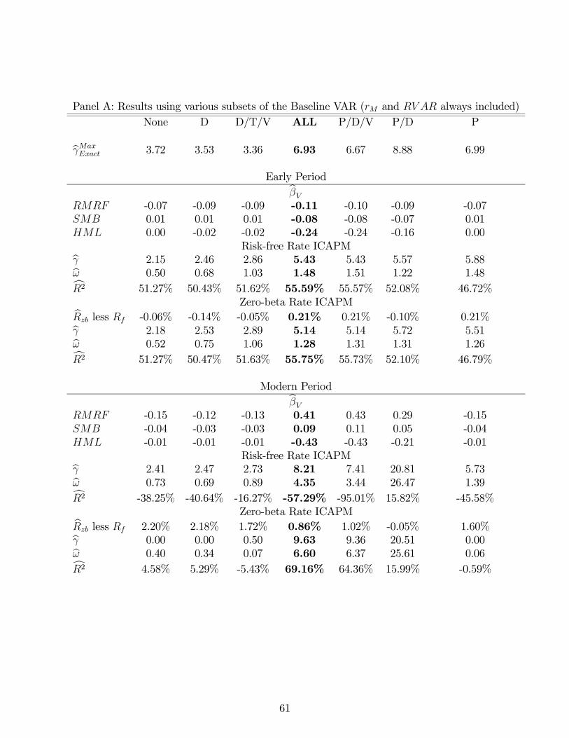
Panel A: Results using various subsets of the Baseline VAR ( and always included)

None D D/T/V ALL P/D/V P/D P

b 3.72 3.53 3.36 6.93 6.67 8.88 6.99

Early Periodb -0.07 -0.09 -0.09 -0.11 -0.10 -0.09 -0.07

0.01 0.01 0.01 -0.08 -0.08 -0.07 0.01

0.00 -0.02 -0.02 -0.24 -0.24 -0.16 0.00

Risk-free Rate ICAPMb 2.15 2.46 2.86 5.43 5.43 5.57 5.88b 0.50 0.68 1.03 1.48 1.51 1.22 1.48c2 51.27% 50.43% 51.62% 55.59% 55.57% 52.08% 46.72%

Zero-beta Rate ICAPMb less -0.06% -0.14% -0.05% 0.21% 0.21% -0.10% 0.21%b 2.18 2.53 2.89 5.14 5.14 5.72 5.51b 0.52 0.75 1.06 1.28 1.31 1.31 1.26c2 51.27% 50.47% 51.63% 55.75% 55.73% 52.10% 46.79%

Modern Periodb -0.15 -0.12 -0.13 0.41 0.43 0.29 -0.15

-0.04 -0.03 -0.03 0.09 0.11 0.05 -0.04

-0.01 -0.01 -0.01 -0.43 -0.43 -0.21 -0.01

Risk-free Rate ICAPMb 2.41 2.47 2.73 8.21 7.41 20.81 5.73b 0.73 0.69 0.89 4.35 3.44 26.47 1.39c2 -38.25% -40.64% -16.27% -57.29% -95.01% 15.82% -45.58%

Zero-beta Rate ICAPMb less 2.20% 2.18% 1.72% 0.86% 1.02% -0.05% 1.60%b 0.00 0.00 0.50 9.63 9.36 20.51 0.00b 0.40 0.34 0.07 6.60 6.37 25.61 0.06c2 4.58% 5.29% -5.43% 69.16% 64.36% 15.99% -0.59%

61

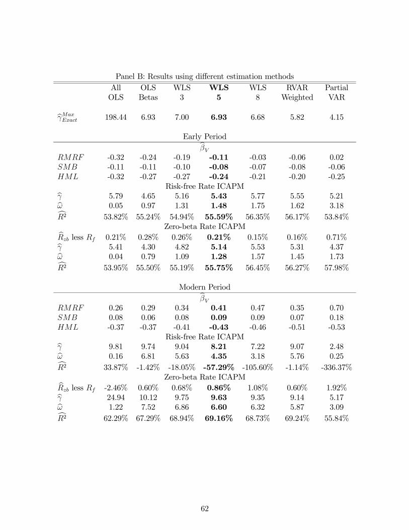
Panel B: Results using different estimation methods

All OLS WLS WLS WLS RVAR Partial

OLS Betas 3 5 8 Weighted VAR

b 198.44 6.93 7.00 6.93 6.68 5.82 4.15

Early Periodb -0.32 -0.24 -0.19 -0.11 -0.03 -0.06 0.02

-0.11 -0.11 -0.10 -0.08 -0.07 -0.08 -0.06

-0.32 -0.27 -0.27 -0.24 -0.21 -0.20 -0.25

Risk-free Rate ICAPMb 5.79 4.65 5.16 5.43 5.77 5.55 5.21b 0.05 0.97 1.31 1.48 1.75 1.62 3.18c2 53.82% 55.24% 54.94% 55.59% 56.35% 56.17% 53.84%

Zero-beta Rate ICAPMb less 0.21% 0.28% 0.26% 0.21% 0.15% 0.16% 0.71%b 5.41 4.30 4.82 5.14 5.53 5.31 4.37b 0.04 0.79 1.09 1.28 1.57 1.45 1.73c2 53.95% 55.50% 55.19% 55.75% 56.45% 56.27% 57.98%

Modern Periodb 0.26 0.29 0.34 0.41 0.47 0.35 0.70

0.08 0.06 0.08 0.09 0.09 0.07 0.18

-0.37 -0.37 -0.41 -0.43 -0.46 -0.51 -0.53

Risk-free Rate ICAPMb 9.81 9.74 9.04 8.21 7.22 9.07 2.48b 0.16 6.81 5.63 4.35 3.18 5.76 0.25c2 33.87% -1.42% -18.05% -57.29% -105.60% -1.14% -336.37%

Zero-beta Rate ICAPMb less -2.46% 0.60% 0.68% 0.86% 1.08% 0.60% 1.92%b 24.94 10.12 9.75 9.63 9.35 9.14 5.17b 1.22 7.52 6.86 6.60 6.32 5.87 3.09c2 62.29% 67.29% 68.94% 69.16% 68.73% 69.24% 55.84%

62

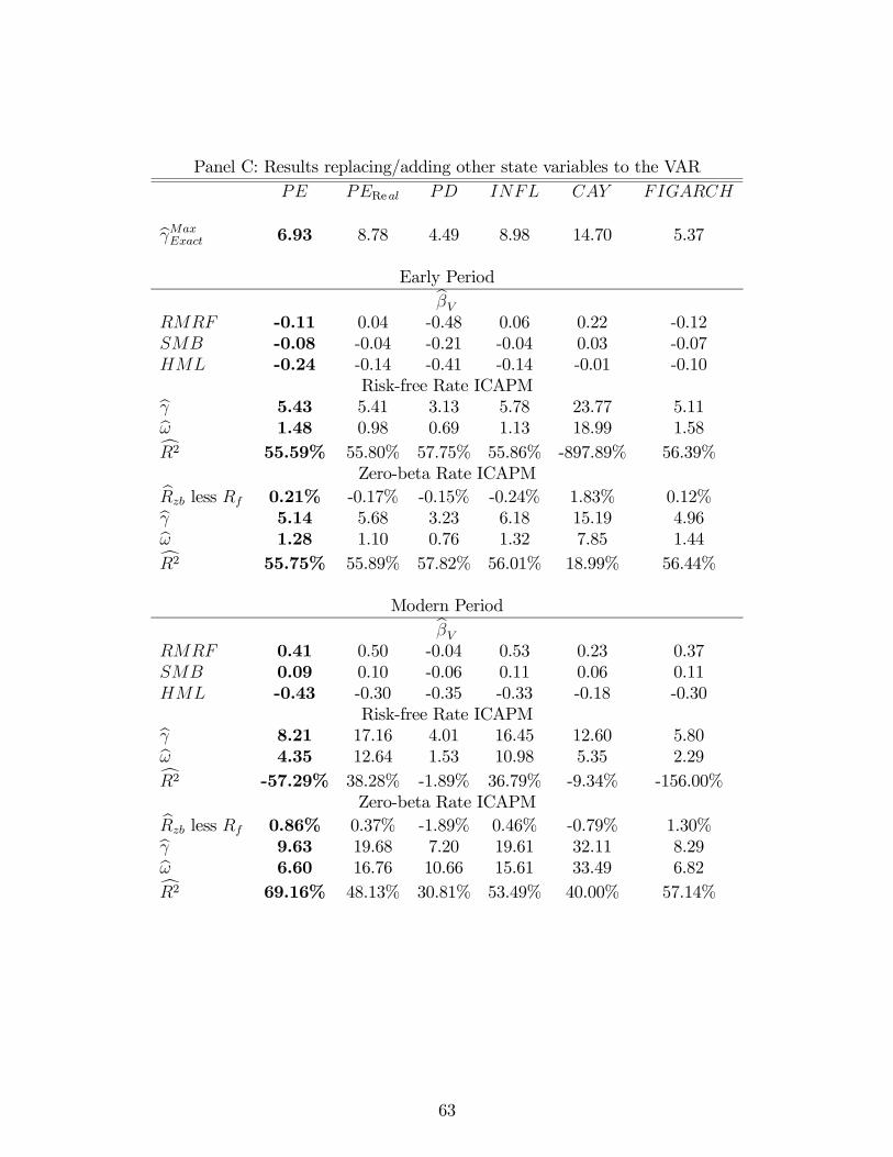
Panel C: Results replacing/adding other state variables to the VAR

Re

b 6.93 8.78 4.49 8.98 14.70 5.37

Early Periodb -0.11 0.04 -0.48 0.06 0.22 -0.12

-0.08 -0.04 -0.21 -0.04 0.03 -0.07

-0.24 -0.14 -0.41 -0.14 -0.01 -0.10

Risk-free Rate ICAPMb 5.43 5.41 3.13 5.78 23.77 5.11b 1.48 0.98 0.69 1.13 18.99 1.58c2 55.59% 55.80% 57.75% 55.86% -897.89% 56.39%

Zero-beta Rate ICAPMb less 0.21% -0.17% -0.15% -0.24% 1.83% 0.12%b 5.14 5.68 3.23 6.18 15.19 4.96b 1.28 1.10 0.76 1.32 7.85 1.44c2 55.75% 55.89% 57.82% 56.01% 18.99% 56.44%

Modern Periodb 0.41 0.50 -0.04 0.53 0.23 0.37

0.09 0.10 -0.06 0.11 0.06 0.11

-0.43 -0.30 -0.35 -0.33 -0.18 -0.30

Risk-free Rate ICAPMb 8.21 17.16 4.01 16.45 12.60 5.80b 4.35 12.64 1.53 10.98 5.35 2.29c2 -57.29% 38.28% -1.89% 36.79% -9.34% -156.00%

Zero-beta Rate ICAPMb less 0.86% 0.37% -1.89% 0.46% -0.79% 1.30%b 9.63 19.68 7.20 19.61 32.11 8.29b 6.60 16.76 10.66 15.61 33.49 6.82c2 69.16% 48.13% 30.81% 53.49% 40.00% 57.14%

63

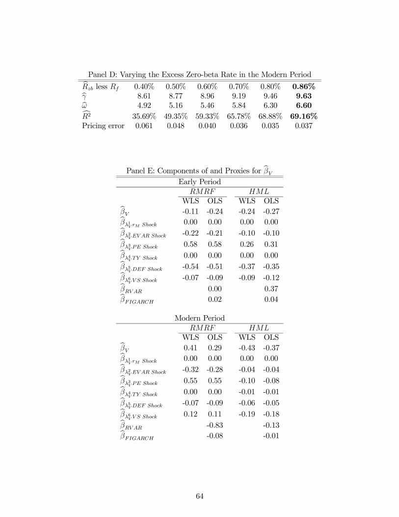
Panel D: Varying the Excess Zero-beta Rate in the Modern Periodb less 0.40% 0.50% 0.60% 0.70% 0.80% 0.86%b 8.61 8.77 8.96 9.19 9.46 9.63b 4.92 5.16 5.46 5.84 6.30 6.60c2 35.69% 49.35% 59.33% 65.78% 68.88% 69.16%

Pricing error 0.061 0.048 0.040 0.036 0.035 0.037

Panel E: Components of and Proxies for bEarly Period

WLS OLS WLS OLSb -0.11 -0.24 -0.24 -0.27b1 0.00 0.00 0.00 0.00b2 -0.22 -0.21 -0.10 -0.10b3 0.58 0.58 0.26 0.31b4 0.00 0.00 0.00 0.00b5 -0.54 -0.51 -0.37 -0.35b6 -0.07 -0.09 -0.09 -0.12b 0.00 0.37b 0.02 0.04

Modern Period

WLS OLS WLS OLSb 0.41 0.29 -0.43 -0.37b1 0.00 0.00 0.00 0.00b2 -0.32 -0.28 -0.04 -0.04b3 0.55 0.55 -0.10 -0.08b4 0.00 0.00 -0.01 -0.01b5 -0.07 -0.09 -0.06 -0.05b6 0.12 0.11 -0.19 -0.18b -0.83 -0.13b -0.08 -0.01

64

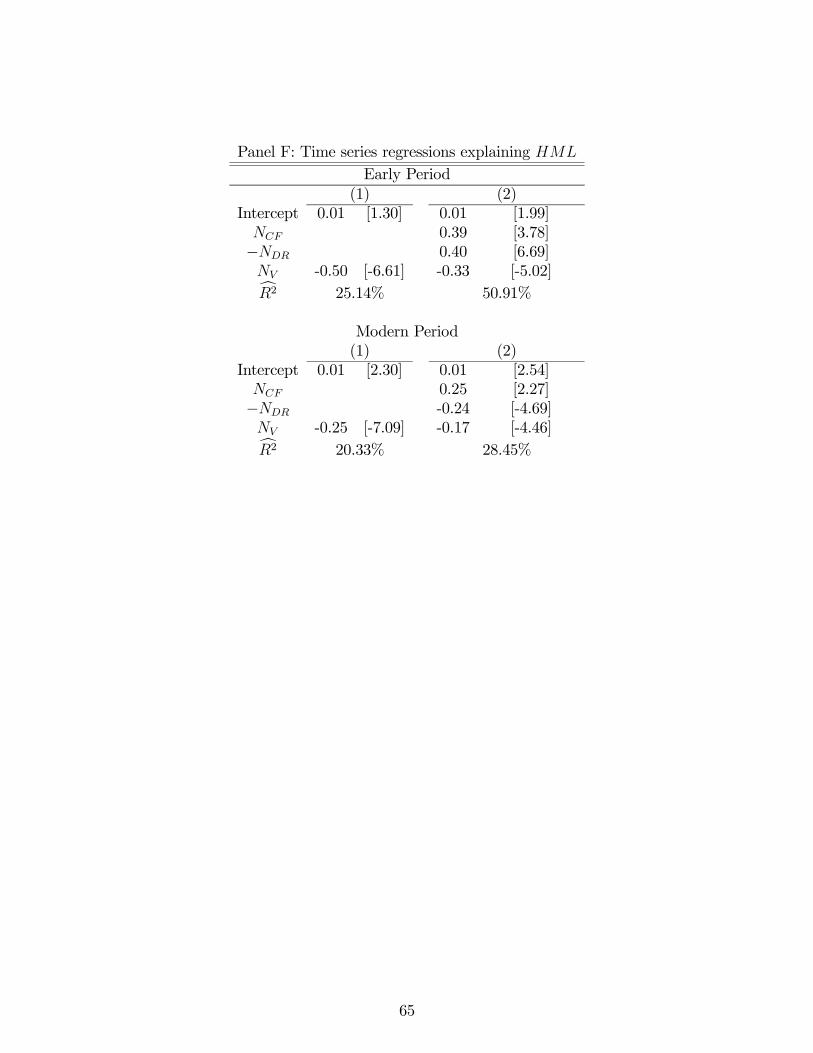
Panel F: Time series regressions explaining

Early Period

(1) (2)

Intercept 0.01 [1.30] 0.01 [1.99]

0.39 [3.78]

− 0.40 [6.69]

-0.50 [-6.61] -0.33 [-5.02]c2 25.14% 50.91%

Modern Period

(1) (2)

Intercept 0.01 [2.30] 0.01 [2.54]

0.25 [2.27]

− -0.24 [-4.69]

-0.25 [-7.09] -0.17 [-4.46]c2 20.33% 28.45%

65

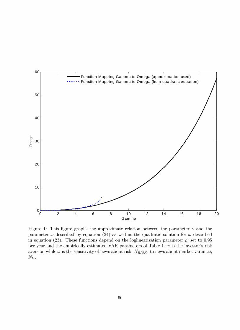
0 2 4 6 8 10 12 14 16 18 200

10

20

30

40

50

60

Om

ega

Gamma

Function Mapping Gamma to Omega (approximation used)Function Mapping Gamma to Omega (from quadratic equation)

Figure 1: This figure graphs the approximate relation between the parameter γ and theparameter ω described by equation (24) as well as the quadratic solution for ω describedin equation (23). These functions depend on the loglinearization parameter ρ, set to 0.95per year and the empirically estimated VAR parameters of Table 1. γ is the investor’s riskaversion while ω is the sensitivity of news about risk, NRISK , to news about market variance,NV .

66

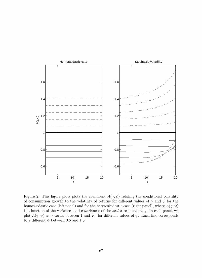
5 10 15 20

0.6

0.8

1

1.2

1.4

1.6

γ

A( γ

, ψ)

Homoskedastic case

5 10 15 20

0.6

0.8

1

1.2

1.4

1.6

γ

Stochastic volati l i ty

Figure 2: This figure plots plots the coeffi cient A(γ, ψ) relating the conditional volatilityof consumption growth to the volatility of returns for different values of γ and ψ for thehomoskedastic case (left panel) and for the heteroskedastic case (right panel), where A(γ, ψ)is a function of the variances and covariances of the scaled residuals ut+1. In each panel, weplot A(γ, ψ) as γ varies between 1 and 20, for different values of ψ. Each line correspondsto a different ψ between 0.5 and 1.5.

67

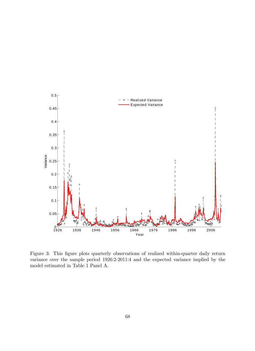
1926 1936 1946 1956 1966 1976 1986 1996 20060

0.05

0.1

0.15

0.2

0.25

0.3

0.35

0.4

0.45

0.5

Varia

nce

Year

Real ized VarianceExpected Variance

Figure 3: This figure plots quarterly observations of realized within-quarter daily returnvariance over the sample period 1926:2-2011:4 and the expected variance implied by themodel estimated in Table 1 Panel A.

68

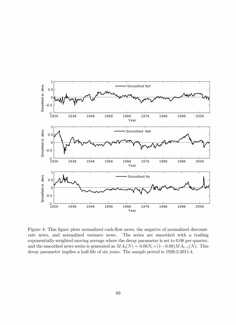
1926 1936 1946 1956 1966 1976 1986 1996 2006­1

­0.5

0

0.5

1

Smoo

thed

 st. 

devs

.

Year

Smoothed Ncf

1926 1936 1946 1956 1966 1976 1986 1996 2006­1

­0.5

0

0.5

1

Smoo

thed

 st. 

devs

.

Year

Smoothed ­Ndr

1926 1936 1946 1956 1966 1976 1986 1996 2006­1

­0.5

0

0.5

1

Smoo

thed

 st. 

devs

.

Year

Smoothed Nv

Figure 4: This figure plots normalized cash-flow news, the negative of normalized discount-rate news, and normalized variance news. The series are smoothed with a trailingexponentially-weighted moving average where the decay parameter is set to 0.08 per quarter,and the smoothed news series is generated asMAt(N) = 0.08Nt+(1−0.08)MAt−1(N). Thisdecay parameter implies a half-life of six years. The sample period is 1926:2-2011:4.

69

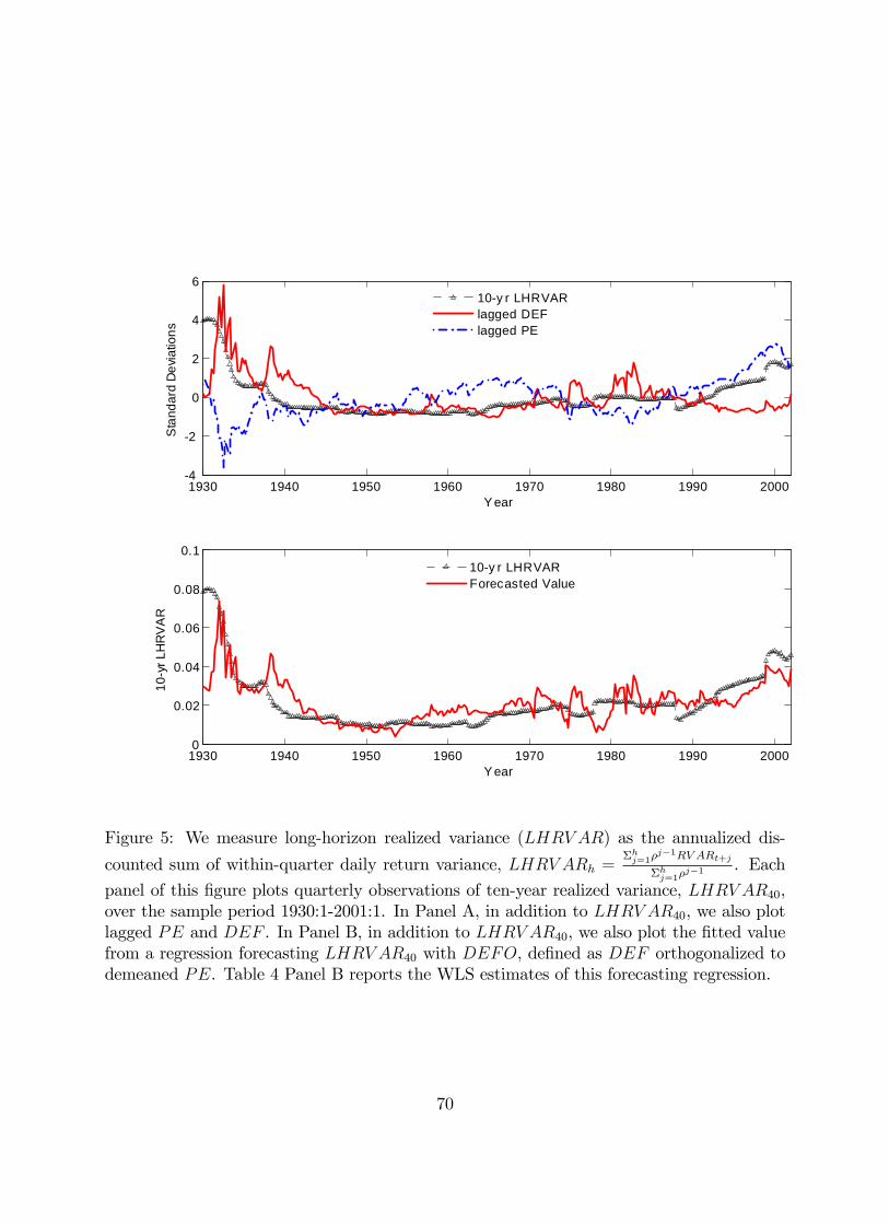
1930 1940 1950 1960 1970 1980 1990 2000­4

­2

0

2

4

6

Sta

ndar

d D

evia

tions

Y ear

10­y r LHRVARlagged DEFlagged PE

1930 1940 1950 1960 1970 1980 1990 20000

0.02

0.04

0.06

0.08

0.1

10­y

r LH

RV

AR

Y ear

10­y r LHRVARForecasted Value

Figure 5: We measure long-horizon realized variance (LHRV AR) as the annualized dis-

counted sum of within-quarter daily return variance, LHRV ARh =Σhj=1ρ

j−1RV ARt+j

Σhj=1ρj−1 . Each

panel of this figure plots quarterly observations of ten-year realized variance, LHRV AR40,over the sample period 1930:1-2001:1. In Panel A, in addition to LHRV AR40, we also plotlagged PE and DEF . In Panel B, in addition to LHRV AR40, we also plot the fitted valuefrom a regression forecasting LHRV AR40 with DEFO, defined as DEF orthogonalized todemeaned PE. Table 4 Panel B reports the WLS estimates of this forecasting regression.

70

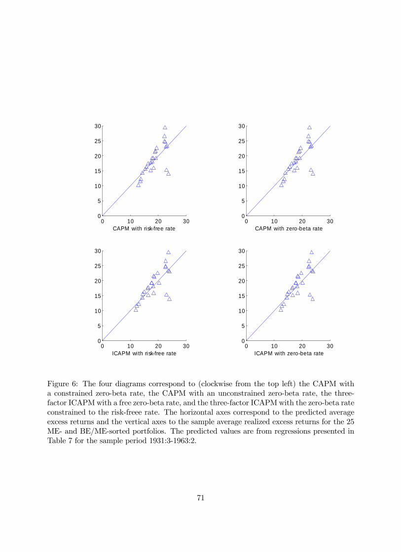
0 10 20 300

5

10

15

20

25

30

ICAPM with zero­beta rate0 10 20 30

0

5

10

15

20

25

30

ICAPM with risk­free rate

0 10 20 300

5

10

15

20

25

30

CAPM with zero­beta rate0 10 20 30

0

5

10

15

20

25

30

CAPM with risk­free rate

Figure 6: The four diagrams correspond to (clockwise from the top left) the CAPM witha constrained zero-beta rate, the CAPM with an unconstrained zero-beta rate, the three-factor ICAPMwith a free zero-beta rate, and the three-factor ICAPMwith the zero-beta rateconstrained to the risk-freee rate. The horizontal axes correspond to the predicted averageexcess returns and the vertical axes to the sample average realized excess returns for the 25ME- and BE/ME-sorted portfolios. The predicted values are from regressions presented inTable 7 for the sample period 1931:3-1963:2.

71

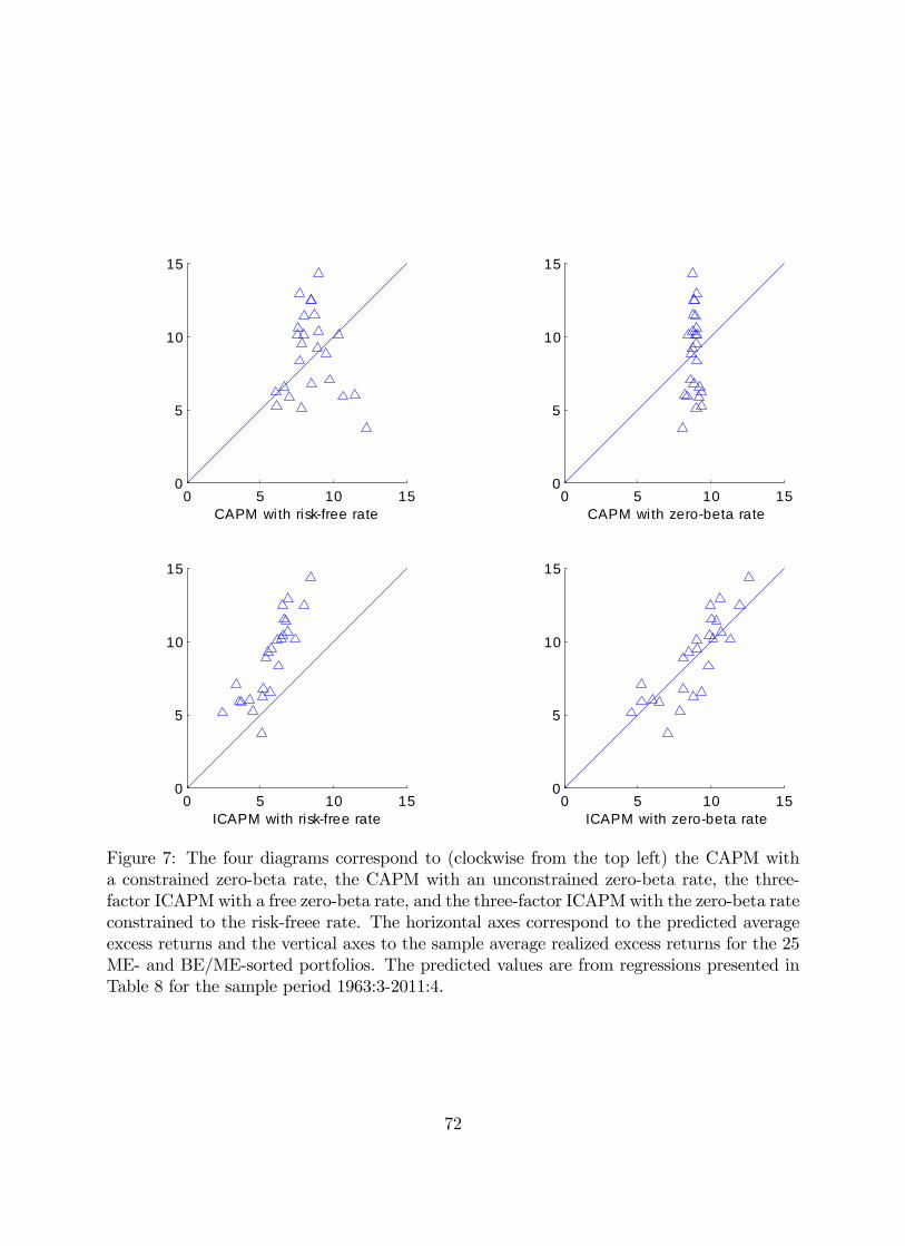
0 5 10 150

5

10

15

ICAPM with zero­beta rate0 5 10 15

0

5

10

15

ICAPM with risk­free rate

0 5 10 150

5

10

15

CAPM with zero­beta rate0 5 10 15

0

5

10

15

CAPM with risk­free rate

Figure 7: The four diagrams correspond to (clockwise from the top left) the CAPM witha constrained zero-beta rate, the CAPM with an unconstrained zero-beta rate, the three-factor ICAPMwith a free zero-beta rate, and the three-factor ICAPMwith the zero-beta rateconstrained to the risk-freee rate. The horizontal axes correspond to the predicted averageexcess returns and the vertical axes to the sample average realized excess returns for the 25ME- and BE/ME-sorted portfolios. The predicted values are from regressions presented inTable 8 for the sample period 1963:3-2011:4.

72

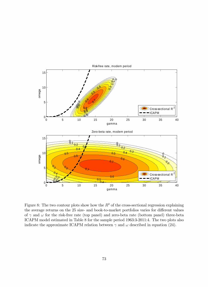
0

0

0

0.1

0.1

0.1

0.2

0.2

0.3

0.30.4

0.4

0.5

0.5

0.6

0.6

0.7

omeg

a

gamma

Risk­free rate, modern period

0 5 10 15 20 25 30 35 400

5

10

15

Cross­sectional R 2

ICAPM

0 0

0

0.1 0.1

0.1

0.1

0.20.2

0.2

0.2

0.30.3

0.30.3

0.40.4

0.4

0.4

0.4

0.5 0.5

0.5

0.5

0.5

0.60.6

0.6

0.6

0.7

0.7

omeg

a

gamma

Zero­beta rate, modern period

0 5 10 15 20 25 30 35 400

5

10

15

Cross­sectional R 2

ICAPM

Figure 8: The two contour plots show how the R2 of the cross-sectional regression explainingthe average returns on the 25 size- and book-to-market portfolios varies for different valuesof γ and ω for the risk-free rate (top panel) and zero-beta rate (bottom panel) three-betaICAPM model estimated in Table 8 for the sample period 1963:3-2011:4. The two plots alsoindicate the approximate ICAPM relation between γ and ω described in equation (24).

73

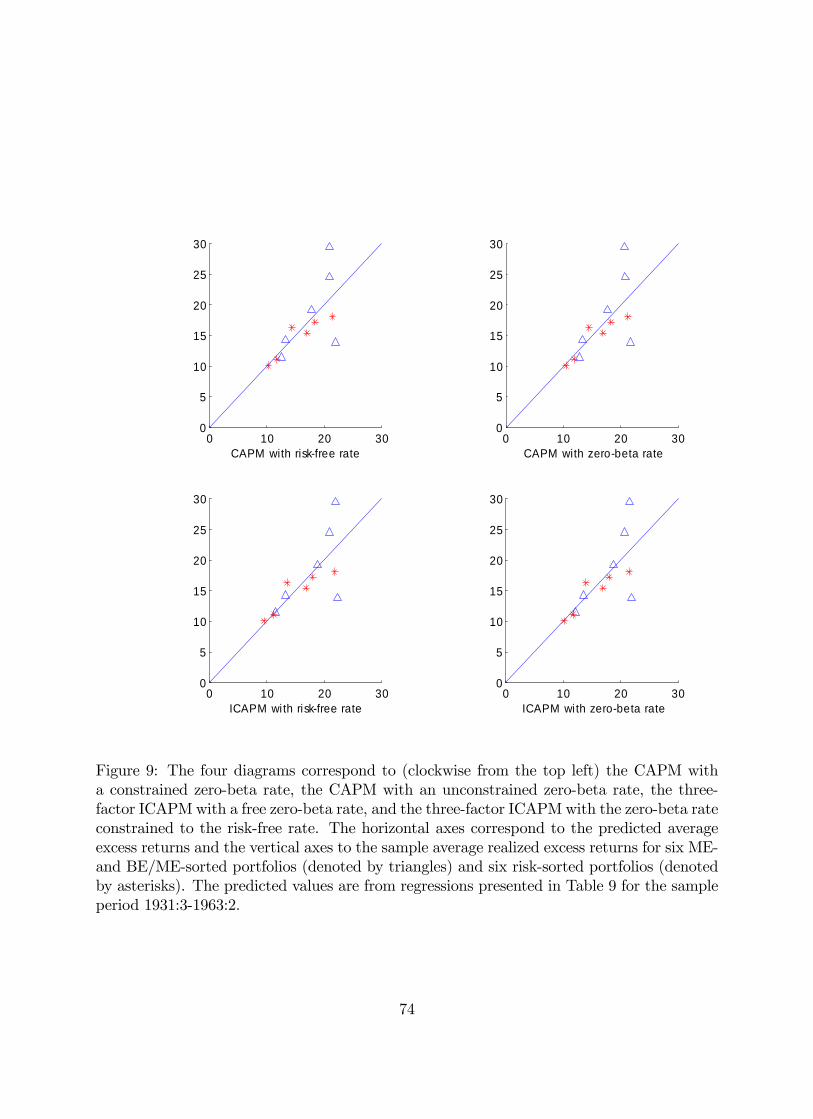
0 10 20 300

5

10

15

20

25

30

ICAPM with zero­beta rate0 10 20 30

0

5

10

15

20

25

30

ICAPM with risk­free rate

0 10 20 300

5

10

15

20

25

30

CAPM with zero­beta rate0 10 20 30

0

5

10

15

20

25

30

CAPM with risk­free rate

Figure 9: The four diagrams correspond to (clockwise from the top left) the CAPM witha constrained zero-beta rate, the CAPM with an unconstrained zero-beta rate, the three-factor ICAPMwith a free zero-beta rate, and the three-factor ICAPMwith the zero-beta rateconstrained to the risk-free rate. The horizontal axes correspond to the predicted averageexcess returns and the vertical axes to the sample average realized excess returns for six ME-and BE/ME-sorted portfolios (denoted by triangles) and six risk-sorted portfolios (denotedby asterisks). The predicted values are from regressions presented in Table 9 for the sampleperiod 1931:3-1963:2.

74

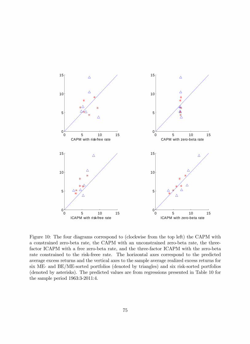
0 5 10 150

5

10

15

ICAPM with zero­beta rate0 5 10 15

0

5

10

15

ICAPM with risk­free rate

0 5 10 150

5

10

15

CAPM with zero­beta rate0 5 10 15

0

5

10

15

CAPM with risk­free rate

Figure 10: The four diagrams correspond to (clockwise from the top left) the CAPM witha constrained zero-beta rate, the CAPM with an unconstrained zero-beta rate, the three-factor ICAPM with a free zero-beta rate, and the three-factor ICAPM with the zero-betarate constrained to the risk-freee rate. The horizontal axes correspond to the predictedaverage excess returns and the vertical axes to the sample average realized excess returns forsix ME- and BE/ME-sorted portfolios (denoted by triangles) and six risk-sorted portfolios(denoted by asterisks). The predicted values are from regressions presented in Table 10 forthe sample period 1963:3-2011:4.

75

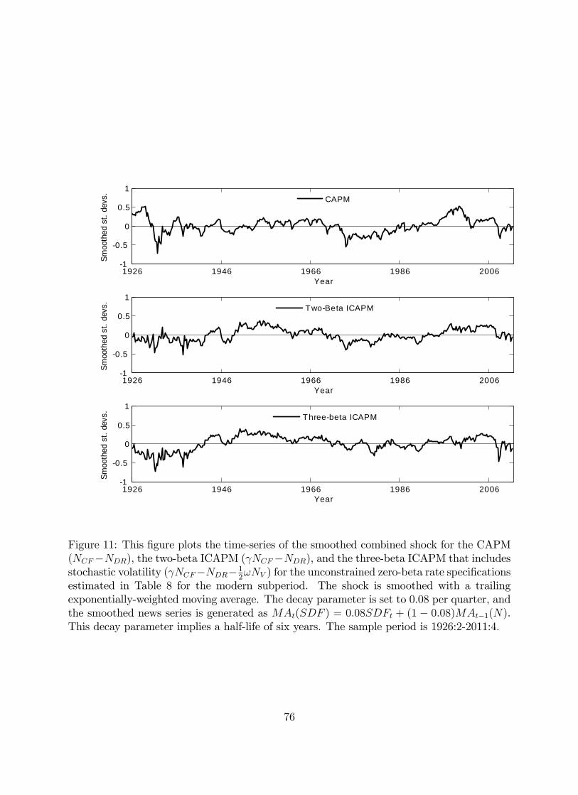
1926 1946 1966 1986 2006­1

­0.5

0

0.5

1

Smoo

thed

 st. 

devs

.

Year

CAPM

1926 1946 1966 1986 2006­1

­0.5

0

0.5

1

Smoo

thed

 st. 

devs

.

Year

Two­Beta ICAPM

1926 1946 1966 1986 2006­1

­0.5

0

0.5

1

Smoo

thed

 st. 

devs

.

Year

Three­beta ICAPM

Figure 11: This figure plots the time-series of the smoothed combined shock for the CAPM(NCF−NDR), the two-beta ICAPM (γNCF−NDR), and the three-beta ICAPM that includesstochastic volatility (γNCF−NDR− 1

2ωNV ) for the unconstrained zero-beta rate specifications

estimated in Table 8 for the modern subperiod. The shock is smoothed with a trailingexponentially-weighted moving average. The decay parameter is set to 0.08 per quarter, andthe smoothed news series is generated as MAt(SDF ) = 0.08SDFt + (1 − 0.08)MAt−1(N).This decay parameter implies a half-life of six years. The sample period is 1926:2-2011:4.

76