An interactive program on digitizing historical seismograms

Yihe Xu a,b,n, Tao Xu a

a State Key Laboratory of Lithospheric Evolution, Institute of Geology and Geophysics, Chinese Academy of Sciences, Beijing 100029, Chinab University of Chinese Academy of Sciences, Beijing 100049, China

a r t i c l e i n f o

Article history:Received 8 May 2013Received in revised form6 October 2013Accepted 4 November 2013Available online 16 November 2013

Keywords:DigitizationInversion problemMatlabs GUIPriori information

a b s t r a c t

Retrieving information from analog seismograms is of great importance since they are considered as theunique sources that provide quantitative information of historical earthquakes. We present an algorithmfor automatic digitization of the seismograms as an inversion problem that forms an interactive programusing Matlabs GUI. The program integrates automatic digitization with manual digitization and users caneasily switch between the two modalities and carry out different combinations for the optimal results.Several examples about applying the interactive program are given to illustrate the merits of the method.

& 2013 Elsevier Ltd. All rights reserved.

1. Introduction

Analog seismograms are barely used nowadays, but the impor-tance of them cannot be denied. It has only been around 70 yearssince the digital seismological data was recorded in the 1960s aswell as the advent of WWSSN, while analog records of teleseismicdata can be dated back to 1889 (Stein et al., 1988).If quantitativeinformation could be extracted from these records, seismic eventsrecorded during more than 70 years could be used by Geophysi-cists (Cadek, 1987; Samardjieva et al., 1998; Baskoutas et al., 2000;Bungum et al., 2003; Lee and Benson, 2008; Mezcua et al., 2013).New understandings may be obtained if the seismicity history isconsidered, because these seismic data have a longer period oftime and are crucial for seismological research (Kanamori, 1988).

Digitizing analog seismograms is essential for employing histor-ical recordings but the digitization quality directly affects the validityof final results and interpretation of the historical earthquakes.Adams and Allen (1961) used a device that is originally applied todigitize weather maps for data processing. Bogert (1961) employedequipment that processes speech and visual data for digital versionsof seismograms. With the development of computers' technologyand scanning and image processing techniques, digitization based onraster images scanned from photographic records was presented byTrifunac et al. (1999). Teves-Costa et al. (1999) demonstrated use ofCADcore to vectorize analog seismograms and then converted theimages into unevenly spaced (x, y) pairs by AUTOCAD so as to obtainthe digitized seismograms. Pintore et al. (2005) developed a

vectorization of historical seismograms, named Teseo, which baseson neural networks and Bezier fitting algorithm and provides bothmanual and automatic trace vectorizations of seismograms,

Although several attempts have been made for more than 70years, and great improvements have been achieved, results from theautomatic digitizing programs still have defects in some particularsituations (Trifunac et al., 1973, 1999), which need subsequentcorrections. It may be possible to remove these defects by purelyautomatic digitalization, but it needs extreme works and results inlengthy codes. The automatic tracing is faster, but its result may notbe able to reach the desired quality. Manual digitization may givethe best resolution, but it is time-consuming. The optimal way todigitalize analog seismograms is combination of manual and auto-matic tracing techniques. In this paper, we present a computerprogram that achieves the combination and offers a friendlygraphical user interface, which allows user easily switch betweenthe manual and automatic digitization modalities.

In the following sections, we first talk about the data we used intesting our programs, then give a general principle of automaticdigitization. We described the digitization of seismograms as aninversion problem, in which the raster image acquired from scan-ning the historical seismograms are considered as the “observeddata”, and the digital seismological data saved in a sequence ofamplitude data on evenly spaced time, as the “model parameters”.Finally, we draw some conclusions from our implementations of thecomputer program and actual digitization results.

2. Data

The first step of historical seismograms digitization is scanningthe analog seismograms (Trifunac et al., 1999). The output of

Contents lists available at ScienceDirect

journal homepage: www.elsevier.com/locate/cageo

Computers & Geosciences

0098-3004/$ - see front matter & 2013 Elsevier Ltd. All rights reserved.http://dx.doi.org/10.1016/j.cageo.2013.11.001

n Corresponding author at: State Key Laboratory of Lithospheric Evolution,Institute of Geology and Geophysics, Chinese Academy of Sciences, Beijing100029, China.

E-mail addresses: xuyihe@mail.iggcas.ac.cn, blazing216@163.com (Y. Xu).

Computers & Geosciences 63 (2014) 88–95

scanners is raster images, which are made up of two-dimensionalarrays of pixels. Each pixel could be represented by either onescaled number of grayscale of pixel, or a color triplet with red,green and blue. The historical seismograms, whether it is on thesmoked paper or the photographic record, are often given ingrayscale colors with which our algorithm starts. Any other kindsof images could be converted into the grayscale images in terms ofthe values of red color. The resolution of the scanned image shouldbe high enough to retain information sufficient for the laterprocessing of digitization. In this study, we focused on the imagesthat have 300 dpi and higher, since they may hold sufficientdetails for refinement of digitization results.

The historical seismograms are recorded by mechanical instru-ments, and result in images that have several characteristics, someof which increase the complexity of the problem, e.g. curvaturedistortion. The algorithm we presented here is based on theassumption that amplitude of seismic traces has a bijectiverelationship with the ordinate values, which corresponds to time.This assumption fails when dealing with the seismograms onsmoked paper due to the curvature distortion (Batlló et al., 2008;Batlló, 2010; Schlupp and Cisternas, 2007). Therefore, the seismo-grams on the smoked paper must be particularly processed, e.g.migrating the pixels to the corrected position to reduce curvaturedistortion. The amount of correction of a pixel is a function ofthe distance between the pixel and the base line of the trace.The function might be obtained from analysis of the structure ofthe seismometer, or the curvature of the seismogram. We assumethat the correction is already completed so that the seismogramssatisfy the “bijective” assumption. We gave two examples to showcapability of our program. One is a seismogram (Fig. 7) on thephotographic record obtained from the paper of Pintore et al.(2005), another comes from rasterization of vector image of wideangle reflection/refraction data (Fig. 6). Although it is not historicalseismograms, it has similar characteristics to the historical ones(those characteristics are discussed in the Section 3). The twoexamples may represent two kinds of seismograms which can beprocessed by our computer program. It should be mentioned thatsome modern seismograms may also need re-digitization to recoverpartial miss in the original data. Our program was originallydeveloped to digitize wide-angle seismic reflection/refraction data.

3. Digitization

3.1. Principle

Considering the digitizing process of seismograms as a blackbox shown in Fig. 1, the input of the black box is a grayscale rasterimage and the output is seismic data. Since we need computers todo the work for us, we should offer a mathematical explanation ofdigitization to the computer. A grayscale raster image is merely atwo-dimensional matrix of which each element has the valueranging from 0 (pure black) to 255 (pure white), and seismic tracesare either parameterized lines (Pintore et al., 2005) or sequencesof time–amplitude pairs (Teves-Costa et al., 1999). Modern seis-mological recording techniques are commonly designed for digitalseismograms that contain amplitude data on evenly spaced time.The sequences of time–amplitude pairs become the format of thedigital seismograms and provide possibility for further numericalprocess and analysis. Hence, the digitization of analog seismo-grams may be simply considered as a procedure that constructs asequence or sequences of doublets from a matrix (image). If wetake the matrix as “observed data” and the sequences of doubletsas “model parameters”, the digitalization becomes an inversionproblem.

The relationship between the model parameters and theobserved data is often defined by a mathematical operator. Math-ematically, the operators must be uniquely determined by the inputmatrix and the output of time–amplitude pairs. However, it isdifficult to give a general and explicit formula of the operatorbecause of the requirement of detailed knowledge of the instru-ment structure that the authors do not have. Alternatively, wechoose a simpler way that regards the forward problem of convert-ing the seismic data to analog seismograms as moving a ballpointpen along the traces on digital seismograms, as shown in Fig. 2.The diameter and shape of the ballpoint pen may vary as it moves. Inaddition, abrupt shift should be involved in case of time marks. Letmk be the kth seismic traces and B be the ballpoint pattern, given by

mk ¼∑Npp ¼ 1δimk

p1δimk

p2; ð1Þ

and

B¼ ½bij�; bij ¼1; if i2þ j2rR2

0; if i2þ j24R2

(; i; j¼ 0; 71; 72;⋯; ð2Þ

respectively. mkp1 and mk

p2 are both integers, and denote the abscissaand the ordinate of the pth point in the kth trace. The raster

Fig. 1. The inversion problem arising in the digitization of historical seismograms.The historical seismograms can be represented by a matrix, whose elements are thegrayscale value of each pixel in the scanned seismograms. The digitized seismictraces are essentially sequences of time–amplitude pairs, which contain theamplitude information in each time point. The black box can refer to any methodwhich can retrieve seismological information from the matrix, and these methodsshould consider the constraints arising from the priori information.

Ballpoint pen pattern (R=3)

Tr

acin

g di

rect

ion

Fig. 2. Illustration of ballpoint pen assumption. The red and green balls representballpoint pen patterns. The red ball is the starting point, and the green ones areautomatic digitization results. An example of pixel representation of ballpointpattern is shown. (For interpretation of the references to color in this figure legend,the reader is referred to the web version of this article.)

Y. Xu, T. Xu / Computers & Geosciences 63 (2014) 88–95 89

seismogram S therefore can be obtained by the convolution of mk

and B, that is

S¼∑Kk ¼ 1Sk ¼∑K

k ¼ 1mknB: ð3Þ

Before comparing the raster seismogram S with the real rastergrayscale seismogram, the following procedures are required.From Eq. (3), we know that the nonzero elements of S correspondto the pixels on the seismic traces. These pixels relates to theblack pixels in common digital seismograms and seismograms onphotographic records, as well to the white pixels in seismogramson smoked papers. For simplicity, we assume that the black pixelscontain seismic information and the white pixels are the back-ground. Assigning 0 and 255 to the nonzero and zero elementsrespectively, one can obtain the result of the forward problem. Theinversion problem is solved by iteratively evaluating the differencebetween the calculated seismograms and the real seismogramsand modifying the traces data until reaching desirable results.

However, there are several factors that affect the inversionresults, e.g. intersections between seismic traces and underminedwidths of seismic traces. Sk in Eq. (3) denotes the seismogramkeeping merely the kth trace, and has the following explicitexpression

ðSkÞij ¼∑Np

p ¼ 1ðδimkp1δjmk

p2ÞnðBijÞ ¼∑Np

p ¼ 1Bi�mkp1 j�mk

p2: ð4Þ

mkp1 and mk

p2 can be simply obtained by deconvolution of Sk.However, if more than one trace is recorded in the seismogram,deconvolution can only obtain the points of the traces withoutdetermining which trace each point belongs to. We thereforeadopt an iterative tracing method to the case. The method startsthe tracing with a point on a trace and tracks down the entiretrace. In each iteration, one new point is selected according to thetraced points and some criteria. These points are considered to beof the same trace. Applying the same method to points on othertraces, one obtains the digitized seismic data. Manual digitizationmodality is also provided in case of any setbacks of the automaticdigitization. We need to emphasize that the application provides agraphic user interface and easy switch between the automatic andmanual digitization modalities. This interactive feature cansignificantly reduce the time on digitization and improve thequality of the final digitized seismograms.

3.2. Automatic digitization

The digitization described above is an underdetermined pro-blem that has nonunique solutions. To overcome this problem, ouriterative algorithm contains a selection of the next point on thetrace in each iteration. The selection is accomplished according tothe following features:

1. Amplitude of seismic traces are bijective functions of time;2. Seismic traces are continuous;3. Seismic traces are smooth (this feature will be lost in low

resolution scanned images of seismograms);4. Seismic traces are energy-limited, i.e. amplitude should be

limited within a proper bound;5. Seismic traces may have varied width;6. Some seismographs give constant width of traces.

These points are common characteristics of seismic traces,despite that they may fail due to some reasons. Consequently,we follow these features and construct the method to select thenext point along the trace.

The algorithmwe present here takes a raster image obtained byscanning the analog seismograms or rasterizing of the digitalseismograms as an input. The image often has many blemishes,

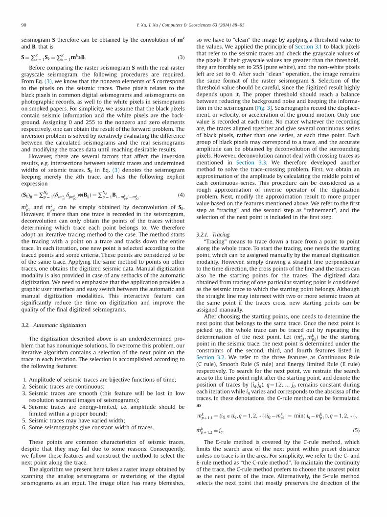
so we have to “clean” the image by applying a threshold value tothe values. We applied the principle of Section 3.1 to black pixelsthat refer to the seismic traces and check the grayscale values ofthe pixels. If their grayscale values are greater than the threshold,they are forcibly set to 255 (pure white), and the non-white pixelsleft are set to 0. After such “clean” operation, the image remainsthe same format of the raster seismogram S. Selection of thethreshold value should be careful, since the digitized result highlydepends upon it. The proper threshold should reach a balancebetween reducing the background noise and keeping the informa-tion in the seismogram (Fig. 3). Seismographs record the displace-ment, or velocity, or acceleration of the ground motion. Only onevalue is recorded at each time. No mater whatever the recordingare, the traces aligned together and give several continuous seriesof black pixels, rather than one series, at each time point. Eachgroup of black pixels may correspond to a trace, and the accurateamplitude can be obtained by deconvolution of the surroundingpixels. However, deconvolution cannot deal with crossing traces asmentioned in Section 3.3. We therefore developed anothermethod to solve the trace-crossing problem. First, we obtain anapproximation of the amplitude by calculating the middle point ofeach continuous series. This procedure can be considered as arough approximation of inverse operator of the digitizationproblem. Next, modify the approximation result to more propervalue based on the features mentioned above. We refer to the firststep as “tracing” and the second step as “refinement”, and theselection of the next point is included in the first step.

3.2.1. Tracing“Tracing” means to trace down a trace from a point to point

along the whole trace. To start the tracing, one needs the startingpoint, which can be assigned manually by the manual digitizationmodality. However, simply drawing a straight line perpendicularto the time direction, the cross points of the line and the traces canalso be the starting points for the traces. The digitized dataobtained from tracing of one particular starting point is consideredas the seismic trace to which the starting point belongs. Althoughthe straight line may intersect with two or more seismic traces atthe same point if the traces cross, new starting points can beassigned manually.

After choosing the starting points, one needs to determine thenext point that belongs to the same trace. Once the next point ispicked up, the whole trace can be traced out by repeating thedetermination of the next point. Let ðmk

p1;mkp2Þ be the starting

point in the seismic trace, the next point is determined under theconstraints of the second, third, and fourth features listed inSection 3.2. We refer to the three features as Continuous Rule(C rule), Smooth Rule (S rule) and Energy limited Rule (E rule)respectively. To search for the next point, we restrain the searcharea to the time point right after the starting point, and denote theposition of traces by (iq,jq), q¼1,2,…. jp remains constant duringeach iteration while iq varies and corresponds to the abscissa of thetraces. In these denotations, the C-rule method can be formulatedas

mkpþ1;1 ¼ fiQ Afiq; q¼ 1;2;⋯gjiQ �mk

p1j ¼ minðjiq�mkp1jÞ; q¼ 1;2;⋯g;

mkpþ1;2 ¼ jq: ð5Þ

The E-rule method is covered by the C-rule method, whichlimits the search area of the next point within preset distanceunless no trace is in the area. For simplicity, we refer to the C- andE-rule method as “the C-rule method”. To maintain the continuityof the trace, the C-rule method prefers to choose the nearest pointas the next point of the trace. Alternatively, the S-rule methodselects the next point that mostly preserves the direction of the

Y. Xu, T. Xu / Computers & Geosciences 63 (2014) 88–9590

trace, for which the mathematical formula is

mkpþ1;1 ¼ fiQ Afiq; q¼ 1;2;⋯gjjiQ �skp1j ¼ minðjiq�skp1jÞ; q¼ 1;2;⋯g

mkpþ1;2 ¼ jq ð6Þ

Here skp1 represents the predicted abscissa value of the next pointbased on the last few points of the trace. We used linear regressionof at most twenty points to obtain the direction of the trace andthen predicted the position of the next point in our program. Userscan switch between the two methods by clicking the checkbox“Smooth” in the program.

The direction of tracing can be set to the direction of timeincreasing or decreasing by assigning mk

p;2þ1 or mkp;2�1 to jq,

respectively. Hence, the whole seismic trace can be obtained wher-ever the starting point is. We included both two-direction tracingmethod to automatically find the starting points and digitize all thetraces, and one-direction tracing method to integrate with the manualdigitization of complicated traces. When the automatic digitizationfails, we use the manual digitization to lead the process through thedifficult area and then continue the automatic digitization.

Both the C- and S-rule methods can get good results for simpleseismograms, in which each seismic trace is isolated from others(Fig. 3). However, such simple traces barely exist in practice.In most of the seismograms, the amplitude of a trace increasesand intersects with other traces when a signal arrives, e.g.,primary waves. Applying the S-rule method to these cases maysolve most of the intersection problems. Similar methods havebeen performed well on digitizing historical seismograms (Pintoreet al., 2005). Although the S-rule method seems better and morenatural than the C-rule method, we included the C-rule method inour program for completeness, because that the C-rule method

essentially depends upon the first-order feature of the traces,while the S-rule method rests on the second-order feature of thetrace. If the raster image has infinite high resolution, the S-rulemethod is the only right choice. However, as the resolutiondecreases, the reliability of the second-order feature diminishes.It changes the smooth seismic traces into pulse-like curves, whichreduce or completely eliminate the smooth characteristic of thetraces. In this case, the S-rule method maybe come even worsethan the C-rule method, which may yields acceptable results inmost of the cases. Therefore, the C-rule method is the defaultautomatic digitization method of our program. The S-rule methodis provided as an additional option for better results in someparticular cases.

3.2.2. RefinementAfter the “tracing” step, we obtain a primary result of automatic

digitization. The quality of the primary results varies amongdifferent images, and few of them are satisfactory. Further refine-ments are needed to improve the quality to meet the requirementof the modern seismological techniques. Actually, our digitaliza-tion described above is based on the abstraction that seismogramsare convolution of seismic data and ball-like patterns. The auto-matic refinements also apply this principle.

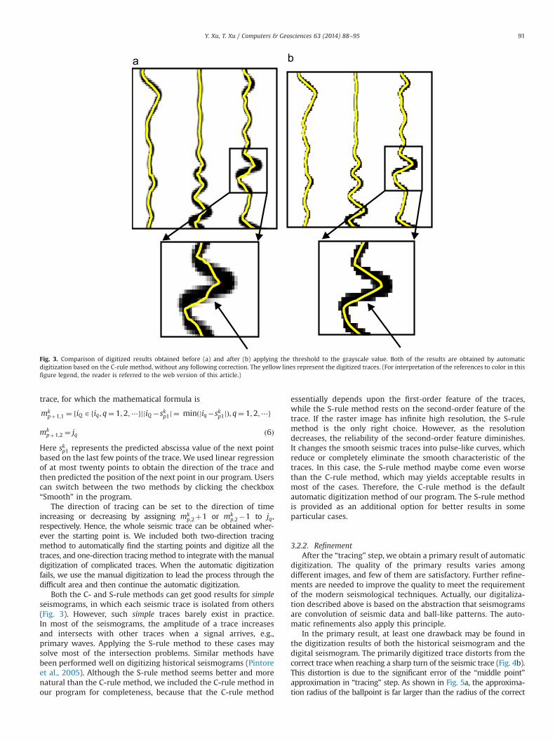
In the primary result, at least one drawback may be found inthe digitization results of both the historical seismogram and thedigital seismogram. The primarily digitized trace distorts from thecorrect trace when reaching a sharp turn of the seismic trace (Fig. 4b).This distortion is due to the significant error of the “middle point”approximation in “tracing” step. As shown in Fig. 5a, the approxima-tion radius of the ballpoint is far larger than the radius of the correct

Fig. 3. Comparison of digitized results obtained before (a) and after (b) applying the threshold to the grayscale value. Both of the results are obtained by automaticdigitization based on the C-rule method, without any following correction. The yellow lines represent the digitized traces. (For interpretation of the references to color in thisfigure legend, the reader is referred to the web version of this article.)

Y. Xu, T. Xu / Computers & Geosciences 63 (2014) 88–95 91

ballpoint (Fig. 5c). Applying variable radii of the ballpoint patternsalong the trace, we obtain the results of “varied width correction”.This correction is the first choice of refinement, which finds thelargest ballpoint pattern internally tangential to the trace with theorigin of the ballpoint at the same time point. “Internally tangential”means that these balls locate inside seismic traces and are infinitely

close to the two boundary lines of the traces (Fig. 5b). This correctionis implemented by bisection search so as to greatly improve the resultnear the peaks or valleys of the seismic traces (Fig. 4). It is suitable forboth the historical seismogram and the modern digital seismograms.The digitized result of historical seismograms after the “varied widthcorrection” now becomes the best one of the automatic digitization.

Fig. 4. The “varied width correction”. Panel (a) illustrates how the refinement works. The red dotted circles with an “� ” at their centers represent solutions during thebisection search, while the green solid circle with a ball at its center represents the final solution. Panels (b) and (c) show the difference between digitization results beforeand after the correction respectively. (For interpretation of the references to color in this figure legend, the reader is referred to the web version of this article.)

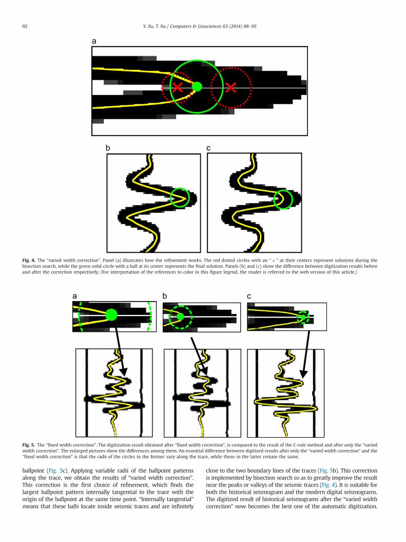
Fig. 5. The “fixed width correction”. The digitization result obtained after “fixed width correction”, is compared to the result of the C-rule method and after only the “variedwidth correction”. The enlarged pictures show the differences among them. An essential difference between digitized results after only the “varied width correction” and the“fixed width correction” is that the radii of the circles in the former vary along the trace, while those in the latter remain the same.

Y. Xu, T. Xu / Computers & Geosciences 63 (2014) 88–9592

Any other distortions are left to manual digitization and the additionalcorrection may be applied.

However, further refinement could be employed to the moderndigital seismograms. Applying a constant radius of the ballpointpattern, we obtain the results of “fixed width correction”, which isalso set up in the program as the second choice of the refinement.The fixed radius takes the dominant radius of the “varied widthcorrection”. Generally, the dominant radius should be smaller thanany other radii. Since the ballpoint patterns after the “varied widthcorrection” are internally tangential to the traces, reduction in theradii makes them close to one boundary of the traces. In order tokeep the amplitude information, we make the ballpoint patternsremain touching the farther boundary away from zero base lines ofthe seismic traces (Fig. 5c). The base line may be obtained indifferent ways, such as mean of the silent part of the trace and themode of the amplitude of the trace. We prefer the second method..

In summary, the automatic digitization algorithm consists offour steps.

Step 1: find the starting point;Step 2: trace along the seismic trace;Step 3: the refinement based on the “varied width correction”(optional);Step 4: the further refinement based on the “varied widthcorrection” (optional).

3.3. Manual digitization

Although the automatic digitization algorithm performs wellon most of the cases, it fails sometimes due to complexity of realseismograms. Leaving the rotation and tilt problem to the pre-digitization process, we concentrate on the problems of the trace-crossing and discontinuity. We have tried to solve the problems inautomatic tracing step by predicting the position of the next pointbased on smoothness feature and have obtained good results.

However, we fail in some complex cases. The problems seemunable to be completely solved by any single algorithm. Wetherefore put a manual digitization into the program to makethe final refinement to the digitized seismograms. The manualdigitization simply records the positions of mouse clicks andinterpolates the positions into a sequence of amplitude–time pairs.It then updates the amplitude data of the corresponding time. Theprograms provide a smooth switch between manual digitizationand automatic one. After the manual digitization, the program canperform a new automatic digitization that starts with the lastpoint of the manual digitization. Then, users can make newmanual correction and automatic digitization. The automaticdigitization here is implemented with one-direction digitizationof a trace. The preferred direction is consistent with the directionof time-increasing.

4. Examples

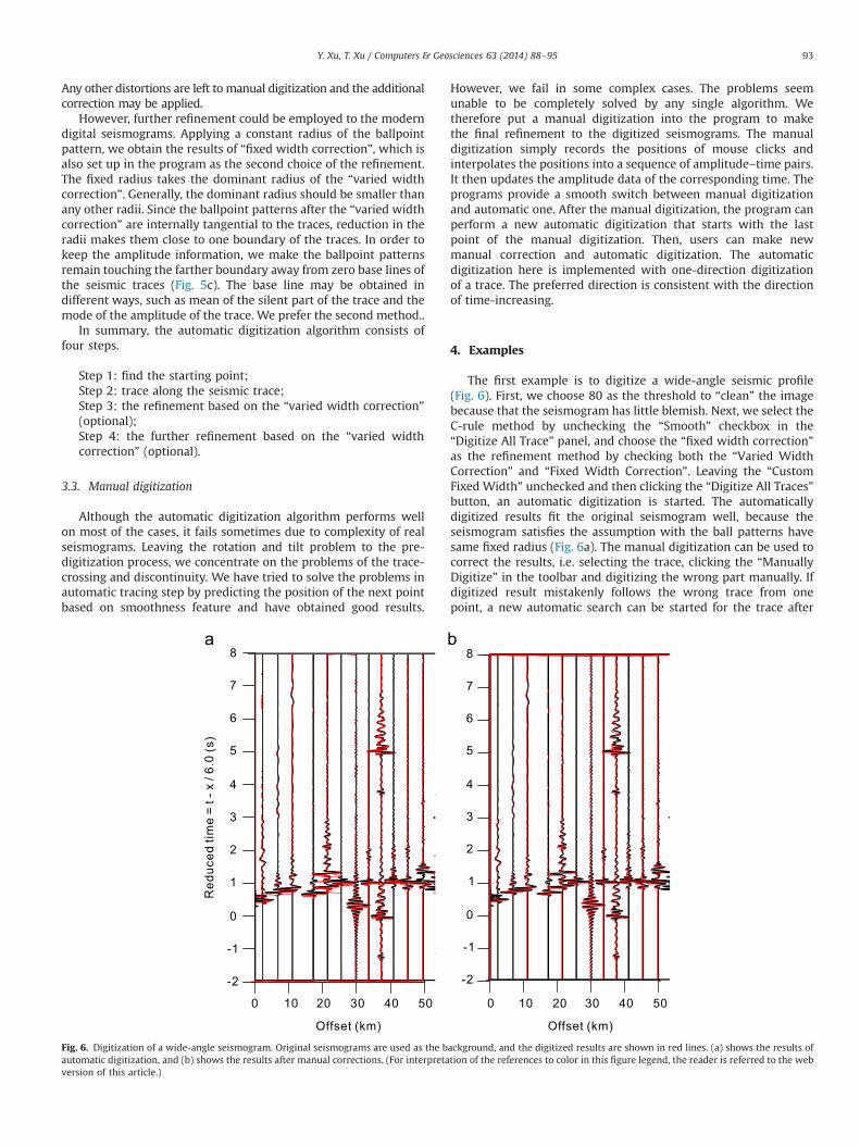
The first example is to digitize a wide-angle seismic profile(Fig. 6). First, we choose 80 as the threshold to “clean” the imagebecause that the seismogram has little blemish. Next, we select theC-rule method by unchecking the “Smooth” checkbox in the“Digitize All Trace” panel, and choose the “fixed width correction”as the refinement method by checking both the “Varied WidthCorrection” and “Fixed Width Correction”. Leaving the “CustomFixed Width” unchecked and then clicking the “Digitize All Traces”button, an automatic digitization is started. The automaticallydigitized results fit the original seismogram well, because theseismogram satisfies the assumption with the ball patterns havesame fixed radius (Fig. 6a). The manual digitization can be used tocorrect the results, i.e. selecting the trace, clicking the “ManuallyDigitize” in the toolbar and digitizing the wrong part manually. Ifdigitized result mistakenly follows the wrong trace from onepoint, a new automatic search can be started for the trace after

Fig. 6. Digitization of a wide-angle seismogram. Original seismograms are used as the background, and the digitized results are shown in red lines. (a) shows the results ofautomatic digitization, and (b) shows the results after manual corrections. (For interpretation of the references to color in this figure legend, the reader is referred to the webversion of this article.)

Y. Xu, T. Xu / Computers & Geosciences 63 (2014) 88–95 93

adjusting the digitized result to the right trace manually. The finalresult of the digitized seismogram is given in Fig. 6b, which shows thedigitalization matches well with the original seismogram (red lines).

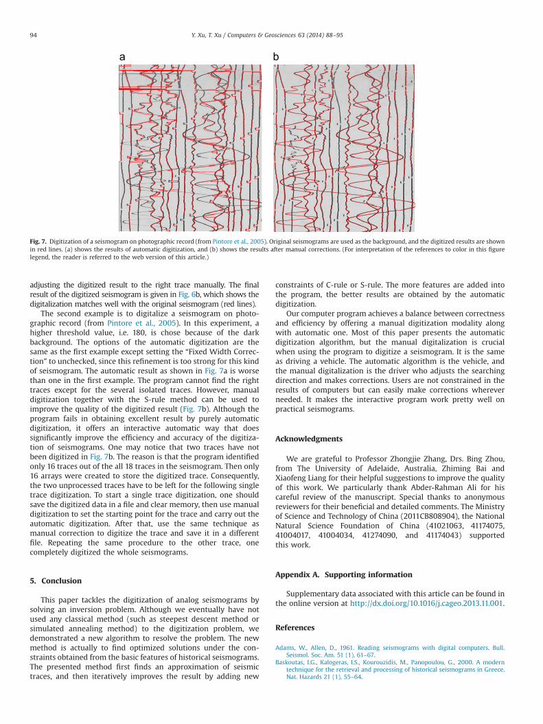
The second example is to digitalize a seismogram on photo-graphic record (from Pintore et al., 2005). In this experiment, ahigher threshold value, i.e. 180, is chose because of the darkbackground. The options of the automatic digitization are thesame as the first example except setting the “Fixed Width Correc-tion” to unchecked, since this refinement is too strong for this kindof seismogram. The automatic result as shown in Fig. 7a is worsethan one in the first example. The program cannot find the righttraces except for the several isolated traces. However, manualdigitization together with the S-rule method can be used toimprove the quality of the digitized result (Fig. 7b). Although theprogram fails in obtaining excellent result by purely automaticdigitization, it offers an interactive automatic way that doessignificantly improve the efficiency and accuracy of the digitiza-tion of seismograms. One may notice that two traces have notbeen digitized in Fig. 7b. The reason is that the program identifiedonly 16 traces out of the all 18 traces in the seismogram. Then only16 arrays were created to store the digitized trace. Consequently,the two unprocessed traces have to be left for the following singletrace digitization. To start a single trace digitization, one shouldsave the digitized data in a file and clear memory, then use manualdigitization to set the starting point for the trace and carry out theautomatic digitization. After that, use the same technique asmanual correction to digitize the trace and save it in a differentfile. Repeating the same procedure to the other trace, onecompletely digitized the whole seismograms.

5. Conclusion

This paper tackles the digitization of analog seismograms bysolving an inversion problem. Although we eventually have notused any classical method (such as steepest descent method orsimulated annealing method) to the digitization problem, wedemonstrated a new algorithm to resolve the problem. The newmethod is actually to find optimized solutions under the con-straints obtained from the basic features of historical seismograms.The presented method first finds an approximation of seismictraces, and then iteratively improves the result by adding new

constraints of C-rule or S-rule. The more features are added intothe program, the better results are obtained by the automaticdigitization.

Our computer program achieves a balance between correctnessand efficiency by offering a manual digitization modality alongwith automatic one. Most of this paper presents the automaticdigitization algorithm, but the manual digitalization is crucialwhen using the program to digitize a seismogram. It is the sameas driving a vehicle. The automatic algorithm is the vehicle, andthe manual digitalization is the driver who adjusts the searchingdirection and makes corrections. Users are not constrained in theresults of computers but can easily make corrections whereverneeded. It makes the interactive program work pretty well onpractical seismograms.

Acknowledgments

We are grateful to Professor Zhongjie Zhang, Drs. Bing Zhou,from The University of Adelaide, Australia, Zhiming Bai andXiaofeng Liang for their helpful suggestions to improve the qualityof this work. We particularly thank Abder-Rahman Ali for hiscareful review of the manuscript. Special thanks to anonymousreviewers for their beneficial and detailed comments. The Ministryof Science and Technology of China (2011CB808904), the NationalNatural Science Foundation of China (41021063, 41174075,41004017, 41004034, 41274090, and 41174043) supportedthis work.

Appendix A. Supporting information

Supplementary data associated with this article can be found inthe online version at http://dx.doi.org/10.1016/j.cageo.2013.11.001.

References

Adams, W., Allen, D., 1961. Reading seismograms with digital computers. Bull.Seismol. Soc. Am. 51 (1), 61–67.

Baskoutas, I.G., Kalogeras, I.S., Kourouzidis, M., Panopoulou, G., 2000. A moderntechnique for the retrieval and processing of historical seismograms in Greece.Nat. Hazards 21 (1), 55–64.

Fig. 7. Digitization of a seismogram on photographic record (from Pintore et al., 2005). Original seismograms are used as the background, and the digitized results are shownin red lines. (a) shows the results of automatic digitization, and (b) shows the results after manual corrections. (For interpretation of the references to color in this figurelegend, the reader is referred to the web version of this article.)

Y. Xu, T. Xu / Computers & Geosciences 63 (2014) 88–9594

Batlló, J., 2010. Influence of Giulio Grablovitz in Spain: instruments and scientificcorrespondence. Ann. Geophys. 52 (6), 699–707.

Batlló, J., Stich, D., Macià, R., 2008. Quantitative analysis of early seismographrecordings, Historical Seismology. Springer, Berlin, pp. 385–402.

Bogert, B.P., 1961. Seismic data collection, reduction, and digitization. Bull. Seismol.Soc. Am. 51 (4), 515–525.

Bungum, H., Lindholm, C., Dahle, A., 2003. Long-period ground-motions for largeEuropean earthquakes, 1905–1992, and comparisons with stochastic predic-tions. J. Seismol. 7 (3), 377–396.

Cadek, O., 1987. Studying earthquake ground motion in Prague from Wiechertseismograph records. Gerl. Beitr. Geophs. 96, 438–447.

Kanamori, H., 1988. Importance of historical seismograms for geophysical research,Historical Seismograms and Earthquakes of the World, pp. 16–33.

Lee, W.H.K., Benson, R.B., 2008. Making non-digitally-recorded seismogramsaccessible online for studying earthquakes. Historical Seismol.: Interdiscip.Stud. Past Recent Earthq. 2, 403–427.

Mezcua, J., Rueda, J., Blanco, R.G., 2013. Iberian peninsula historical seismicityrevisited: an intensity data bank. Seismol. Res. Lett. 84 (1), 9–18.

Pintore, S., Quintiliani, M., Franceschi, D., 2005. Teseo: a vectoriser of historicalseismograms. Comput. Geosci. 31 (10), 1277–1285.

Samardjieva, E., Payo, G., Badal, J., López, C., 1998. Creation of a digital database forXXth century historical earthquakes occurred in the Iberian area. Pure Appl.Geophys. 152 (1), 139–163.

Schlupp, A., Cisternas, A., 2007. Source history of the 1905 great Mongolianearthquakes (Tsetserleg, Bolnay). Geophys. J. Int. 169 (3), 1115–1131.

Stein, S., Okal, E., Wiens, D., 1988. Application of modern techniques to analysis ofhistorical earthquakes, Historical Seismograms and Earthquakes of the World,pp. 85–104.

Teves-Costa, P., Borges, J., Rio, I., Ribeiro, R., Marreiros, C., 1999. Source parametersof old earthquakes: semi-automatic digitization of analog records and seismicmoment assessment. Nat. Hazards 19 (2-3), 205–220.

Trifunac, M.D., Lee, V.W., Todorovska, M.I., 1999. Common problems in automaticdigitization of strong motion accelerograms. Soil Dyn. Earthq. Eng. 18 (7),519–530.

Trifunac, M.D., Udwadia, F.E., Brady, A.G., 1973. Analysis of errors in digitizedstrong-motion accelerograms. Bull. Seismol. Soc. Am. 63 (1), 157–187.

Y. Xu, T. Xu / Computers & Geosciences 63 (2014) 88–95 95