An Intelligent Method for Sizing Optimization in Grid-connected Photovoltaic System

Available online at www.sciencedirect.com

www.elsevier.com/locate/solener

Solar Energy 86 (2012) 2067–2082

An intelligent method for sizing optimizationin grid-connected photovoltaic system

Shahril Irwan Sulaiman a,⇑, Titik Khawa Abdul Rahman a, Ismail Musirin a,Sulaiman Shaari b, Kamaruzzaman Sopian c

a Faculty of Electrical Engineering, Universiti Teknologi MARA, Selangor, Malaysiab Faculty of Applied Sciences, Universiti Teknologi MARA, Selangor, Malaysia

c Solar Energy Research Institute, Universiti Kebangsaan Malaysia, Selangor, Malaysia

Received 1 February 2012; received in revised form 28 March 2012; accepted 12 April 2012Available online 10 May 2012

Communicated by: Associate Editor Takhir Razykov

Abstract

This paper presents an intelligent sizing technique for sizing grid-connected photovoltaic (GCPV) system using evolutionary program-ming (EP). EP was used to select the optimal set of photovoltaic (PV) module and inverter for the system such that the technical or eco-nomic performance of the system could be optimized. The decision variables for the optimization process are the PV module and inverterwhich had been encoded as specific integers in the respective database. On the other hand, the objective function of the optimization taskwas set to be either to optimize the technical performance or the economic performance of the system. Before implementing the intel-ligent-based sizing algorithm, a conventional sizing model had been presented which later led to the development of an iterative-basedsizing algorithm, known as ISA. As the ISA tested all available combinations of PV modules and inverters to be considered for the sys-tem, the overall sizing process became time consuming and tedious. Therefore, the proposed EP-based sizing algorithm, known as EPSA,was developed to accelerate the sizing process. During the development of EPSA, different EP models had been tested with a non-linearscaling factor being introduced to improve the performance of these models. Results showed that the EPSA had outperformed ISA interms of producing lower computation time. Besides that, the incorporation of non-linear scaling factor had also improved the perfor-mance of all EP models under investigation. In addition, EPSA had also shown the best optimization performance when compared withother intelligent-based sizing algorithms using different types of Computational Intelligence.� 2012 Elsevier Ltd. All rights reserved.

Keywords: Photovoltaic (PV); Grid-connected photovoltaic (GCPV); Sizing; Evolutionary programming (EP); Optimization

1. Introduction

As the conventional fuel resources throughout the worldcontinue to deplete, the renewable energy resources andtechnologies have been widely used to compensate thedepletion of the conventional fuel resources. One of thepromising renewable energy is the PV technology. Using

0038-092X/$ - see front matter � 2012 Elsevier Ltd. All rights reserved.

http://dx.doi.org/10.1016/j.solener.2012.04.009

⇑ Corresponding author.E-mail address: [email protected] (S.I. Sulaiman).

this technology, the solar energy is converted to electricityusing solar cells embedded inside a PV module. Althoughthe photovoltaic effect had been first discovered byEdmond Becquerel in 1839, the principles of the modernsolar cells were only established by Bell Laboratories in1954 during an investigation on the properties of extrinsicsilicon. Since then, many types of solar cells based on dif-ferent crystalline and non-crystalline based technologieshad been designed and manufactured commercially in theform of PV modules. However, the usage of crystallinePV module has become common particularly due to its


mailto:[email protected]


2068 S.I. Sulaiman et al. / Solar Energy 86 (2012) 2067–2082

higher conversion efficiency compared to the non-crystal-line PV modules (Dougherty et al., 2005). In addition,the PV modules are usually combined in a series–parallelcombination to form a PV array which is later connectedto the power conditioning units and other balance of sys-tem components. The interconnection of these componentsforms a PV system that can be used for many applications.

One of the most important applications of PV systems isthe GCPV power system. In GCPV system, the DC elec-tricity generated by PV modules of an array is transferredto an inverter for the conversion of DC power to ACpower. Later, the output power from the inverter is fedto the local utility grid. Thus, the GCPV systems couldbenefit the system owners by reducing their monthly elec-tricity bills from the exported electricity. In addition, thecustomers could still enjoy the electricity from the grid ifthere is no power generated from the system. The usageGCPV systems have become primarily significant in theurban areas where the conventional utility grid networkis readily available. In addition, the application of GCPVpower systems ranges from huge centralized power plantswith very large PV array capacities to the smaller-scale dis-tributed systems with small PV array capacities. However,recent statistics showed that approximately 60% of thetotal installed PV power worldwide had been producedby small distributed GCPV systems (MBIPV, 2009). Thesedistributed systems are commonly installed in commercialand residential buildings. Moreover, a recent growing mar-ket demand for the distributed GCPV systems has gener-ated a lot of interests among the stakeholders of the PVindustries in the various aspects of research and develop-ment, manufacturing, business investment, economics andfinance. As a result, GCPV system presents a promisingmode of distributed power generation.

In spite of the strong potential, one of the most impor-tant issues in GCPV system is the sizing of the systems. If aGCPV system is not properly sized, the system might notbe functioning as expected (Shaari et al., 2010). In addition,since there are many different models of system compo-nents that are commercially available in the market, theselection of the most appropriate system components hasfrequently been a challenging task for the system designers.The selection process, known as sizing, not only involvesthe selection of the PV module and inverter, but also thedetermination of other technical and economic parametersin the design. The sizing task is usually performed eitherintuitively using a prescribed design steps (Shaari et al.,2010) or with the assistance of available software packagesfor specific design applications. Unlike the intuitive designapproach which involves manual calculations, the usage ofsizing software could expedite the overall design process asthe sizing task is performed automatically using the algo-rithms configured in the software. However, although var-ious software-based sizing approaches had been introducedrecently (Turcotte et al., 2001), the usage of these softwareare still limited as the system designers are required to indi-rectly utilize the prescribed sizing algorithms readily

embedded in the software. Due to this limitation, the sizingsoftware has commonly been used as a comparison tool forthe manual sizing results produced by the system designers.In fact, the usage of sizing software still requires intuitiveapproach to ensure that the sizing solution is sensible andacceptable. In contrast, the system designers are alwaysallowed to choose their own design steps using the intuitivemethod. Nevertheless, despite having stronger flexibilitycompared to software-based design, the intuitive designapproach could be time consuming and tedious especiallywhen there are more design options to be evaluated beforeselecting the best solution (Sulaiman et al., 2010).

Due to the limitation presented by the intuitive sizingmethod and the sizing software, Kornelakis and Koutrou-lis (2009) had developed an intelligent sizing optimizationscheme for GCPV system using genetic algorithm (GA).The first step of the sizing process was the selection ofPV module, inverter, climatic parameters, available areadimensions, cost and economy parameters as well as themounting arrangement. Then, a GA optimization proce-dure was executed. The decision variables for the optimiza-tion using GA were the number of PV modules, thenumber of parallel strings and PV module tilt angle whilethe objective function was to maximize the total net profitof the system. However, the type of PV module and inver-ter being selected for the sizing process were not evolved.Later, Kornelakis and Marinakis (2010) had proposed aparticle swarm optimization (PSO)-based technique forsimilar optimization task. At the end of the study, the per-formance of PSO-based sizing was compared with the per-formance of GA-based sizing approach. It was found thatPSO could be implemented using lower number of itera-tions during the optimization. Nevertheless, these studiesdid not include the inverter-to-PV array sizing ratio asone of the design criteria. Moreover, the types of powerlosses being defined in this study were purely the inverterlosses and the MPPT losses. Therefore, the sizing can beconsidered as too simplistic as the losses associated to thetemperature, dirt and cables were excluded from the sizingprocess. In addition, since the tilt angle of PV modules wasevolved during the optimization process, the proposedintelligent techniques were only suitable for the design onflat rooftop where customized tilt angle of the PV modulesupporting structure is possible. In fact, recent study hadshown that PSO was outperformed by artificial immunesystem (AIS) and GA in sizing GCPV system (Sulaimanet al., 2011).

This paper presents an intelligent algorithm for thedesign optimization of GCPV system. This algorithm wasintended to suit the design goal of optimizing the usageof available roof space for the system. Although manyintelligent optimization methods were successfully appliedin renewable energy (Banos et al., 2011; Mellit et al.,2009; Kalogirou, 2001), EP was selected as the optimizerfor the sizing algorithm developed in this study. It was usedto design a system based on pre-determined sets of PVmodule and inverter such that the technical or economic

S.I. Sulaiman et al. / Solar Energy 86 (2012) 2067–2082 2069

performance of the system could be optimized. Besidesthat, different types of EP model had been tested to deter-mine the best EP model for the intelligent sizing algorithm.In addition, a non-linear scaling factor was also proposedwith the aim of improving the optimization performanceof the EP models. The performance of the EP-based sizingalgorithm was later compared with selected intelligent opti-mization methods for validation.

2. Methodology

The scope of this study involves a distributed GCPV sys-tems without energy storage as the installations of such sys-tems are expected to increase for the next decades to come(Thomson and Infield, 2007). In addition, single-phaseinverters with built-in maximum power point (MPPT)trackers and nominal output power rating of less than10 kW had been investigated (Salas and Olıas, 2009).Besides that, the types of PV technology evaluated in thisstudy are the silicon-based mono-crystalline and polycrys-talline PV modules. The crystalline-based PV modules wereinvestigated as they have been widely used (Kjaer et al.,2005). In addition, the production and demand of the crys-talline-based PV modules have shown significant growthglobally ( REN21, 2010; Mafigo, 2007; Hoffmann, 2006).Apart from that, the sizing task was conducted for a pro-spective site in Kuala Lumpur, Malaysia for demonstrationpurpose.

Apart from that, the study was also conducted using aseries of methods. Firstly, a conventional system sizingmodel was presented to provide a basic sizing conceptnot only based on technical aspect, but also on economicaspect. Later, an iterative sizing algorithm was developedbased on the pre-formulated conventional system sizingmodel. The outputs from this model would subsequentlybe the benchmarked results for the proposed intelligent siz-ing algorithm. After that, an EP model with the proposednon-linear scaling factor was presented before an intelli-gent sizing algorithm using EP was developed.

3. GCPV system sizing model

The GCPV system sizing model commonly involves twomajor procedures, namely the technical sizing procedureand economic sizing procedure. The technical sizing proce-dure and economic sizing procedure are executed to deter-mine the expected technical performance indicators and theeconomic performance indicator of the proposed systemrespectively. However, the technical sizing procedure usu-ally precedes the economic sizing procedure. In this study,a conventional sizing algorithm (CSA) was developed inMatlab to represent the system sizing model. The CSAwas formulated based on a sizing task using a pre-selectedset of PV module and inverter. In addition, sizing based ona prospective rooftop in Kuala Lumpur, Malaysia hadbeen assumed. The rooftop was also assumed to have a tiltangle of 15� facing South. Besides that, the goal of the siz-

ing task used in this study was to maximize the energy out-put from an available roof space. The technical sizingprocedure was implemented using the following steps:

� Step 1: Select a PV module and an inverter. At thisstage, the respective ratings for these components shouldbe identified for the sizing process. The required ratingsof the PV module were the maximum power in Wp,Pmp_stc, voltage at maximum power, Vmp_stc, open circuitvoltage, Voc_stc, short circuit current, Isc_stc, temperaturecoefficient for maximum power, cPmp, temperature coef-ficient for voltage at maximum power, cVmp, tempera-ture coefficient for open circuit voltage, cVoc, reductionfactor for array output due to manufacturer’s tolerancein decimals, fmm, maximum allowable system voltage ofPV array in V, Vsys_max, length of PV module in m, Lmod,and width of PV module in m, Wmod with all electricalratings rated at standard test conditions (STC). TheSTC specifies that the respective module ratings areobtained at irradiance of 1000 Wm�2, air mass (AM)of 1.5 and cell temperature of 25 �C (Skoplaki and Paly-vos, 2009). On the other hand, the required inverter rat-ings were nominal power of inverter in W, Pinv,maximum input voltage of inverter in V, Vmax_inv, max-imum input voltage limit to the MPPT of inverter in V,Vmax_win_inv, minimum input voltage limit to the MPPTof inverter in V, Vmin_win_inv, maximum input current tothe inverter, Idc_max_inv and nominal efficiency of inverterin%, ginv. These ratings represented the main technicalinputs to the sizing process.� Step 2: Revise the input voltage limits to the MPPT of

inverter to ensure that the output voltage from the PVarray would always be within the input voltage range ofthe inverter. The revised voltage limits were the revisedmaximum input voltage of inverter in V, Vmax_inv_rev,revised maximum input voltage limit to the MPPT ofinverter in V, Vmax_win_inv_rev, and revised minimum inputvoltage limit to the MPPT of inverter in V, Vmin_win_inv_rev.They were computed using

V max inv rev ¼ ð1� kupperÞ � V max inv ð1ÞV max win inv rev ¼ ð1� kupperÞ � V max win inv ð2ÞV min win inv rev ¼ ð1þ klowerÞ � V min win inv ð3Þwhere kupper and klower are the safety margin of the upperlimit and lower limit of the input voltage to the inverterrespectively, described in %. The kupper and klower werechosen to be 5% and 10% respectively as indicated inShaari et al. (2010) after considering the lowest andhighest module temperature recorded in Malaysia.

� Step 3: Determine the extreme output voltages from theexpected PV module by calculating the maximum opencircuit voltage of the PV module in V, Vmax_oc, themaximum voltage at maximum power of the PV modulein V, Vmax_mp, the minimum voltage at maximum powerof the PV module in V, Vmin_mp, and the minimum

(b)(a)

series-connected cells in a string

Parallel strings

series-connected cells in a string

Parallel strings

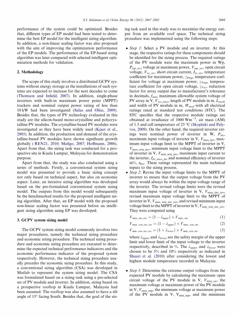
Fig. 1. Difference between (a) lengthwise across and (b) lengthwise uparray mounting arrangement.


voltage at maximum power of the PV module after con-sidering voltage drop in V, Vmin_mp_vd. These voltageswere determined using

V max oc ¼ V oc stc � ½cVoc � ðT cell min � T stcÞ� ð4ÞV max mp ¼ V mp stc � ½cVmp � ðT cell min � T stcÞ� ð5ÞV min mp ¼ V mp stc � ½cVmp � ðT cell max � T stcÞ� ð6ÞV min mp vd ¼ ð1� qÞ � V min mp ð7Þ

where Tcell_min and Tcell_max are the expected minimumand maximum cell temperature in �C respectively. Tcell_-

min and Tcell_max were selected to be 20 �C and 75 �Crespectively (Shaari et al., 2010). In addition, the maxi-mum allowable voltage drop across DC cables, q was se-lected to be 5% as required by the Malaysian StandardMS1837:2010 (Installation of grid-connected photovol-taic (PV) system, 2010).

� Step 4: Determine the minimum and maximum numberof PV modules per string as well as the maximum num-ber of parallel strings which satisfy the inverter voltageand current limits using

Ns;max oc ¼V max inv rev

V max ocð8Þ

Ns;max mp ¼V max win inv rev

V max mpð9Þ

Ns;min ¼V min win inv rev

V min mp vdð10Þ

Np;max ¼Idc max inv

ð1þ xÞ � Isc stcð11Þ

where Ns,max_oc and Ns,max_mp are the maximum numberof PV modules per string based on the open circuit voltageof the PV module and the maximum number of PV mod-ules per string based on the voltage at maximum power ofthe PV module. They were rounded down towards thenearest integer such that the output voltages from thePV array satisfied the respective Vmax_inv and Vmax_win_inv.However, the lower value between Ns,max_oc and Ns,max_mp

was selected as the maximum allowable number of PVmodules per string, Ns,max. On the other hand, the mini-mum allowable number of PV modules per string, Ns,min

was rounded up towards the nearest integer such that theexpected output voltage from the PV array did not fall be-low Vmin_win_inv_rev. Besides that, the maximum allowablenumber of parallel strings, Np,max was rounded down to-wards the nearest integer such that the array current didnot exceed Idc_max_inv. In addition, safety margin for theinput current to the inverter, x is chosen to be 25% asindicated in Shaari et al. (2010) after considering the occa-sionally high irradiance cases with more than 1000 Wm�2

recorded in Malaysia.

� Step 5: Based on Ns,min, Ns,max and Np,max, list all possi-ble array configurations, i.e. the possible number of PV

modules per string, Ns_poss and the possible number par-allel strings, Np_poss with the corresponding total possi-ble number of PV modules, Ntot_poss. Later, the arrayconfigurations with Ntot_poss less than Ntot_est were dis-carded from the list. In addition, for each array config-uration, the system voltage of PV array in V, Vsys wasdetermined using

V sys ¼ Ns poss � V mp stc ð12Þ

If Vsys was greater than Vsys_max, the array configurationwas also discarded from the list.

� Step 6: Determine the actual rated power of PV array inW, Parray_stc_act, for each array configuration using

P array stc act ¼ Ns poss � N p poss � P mp stc ð13Þ

� Step 7: Determine the inverter-to-PV array size ratio,SFinv_pv_act for each array configuration.

SF inv pv act ¼P inv

P array stc actð14Þ

� Step 8: Eliminate the PV array configurations whichproduce SFinv_pv_act values outside a predefined optimalrange. In Malaysia, the optimal range of SFinv_pv_act forsystem with crystalline based PV modules was found tobe from 0.75 to 0.80 (Omar and Shaari, 2009).� Step 9: Determine the maximum number of PV modules

that can be mounted on the available roof space usinglengthwise across (LA) and lengthwise up (LU) by con-sidering a gap between each PV module, lg. The LA isalways preferred compared to LU as the LA couldreduce the effect of dirt or dust accumulation on thePV modules. An illustration of LA and LU is shownin Fig. 1. If the PV modules are installed in LA, onlya string of cells is potentially affected by the dust accu-mulated at the lower section of the module. In contrast,using LU, all parallel strings are potentially affected bythe dust accumulation at the lower section of the mod-ule. Therefore, LA was preferred since only one stringis potentially affected by the dirt.


The maximum number of PV modules that canbe mounted on the available roof space using LA,Nroof_max_LA and the maximum number of PV modulesthat can be mounted on the available roof space usingLU, Nroof_max_LU were computed using

Nroof max LA ¼W roof

ðW mod þ lgÞ� Lroof

ðLmod þ lgÞð15Þ

Nroof max LU ¼W roof

ðLmod þ lgÞ� Lroof

ðW mod þ lgÞð16Þ

� Step 10: If more than one array configurations were left,the Ntot_poss for each array configuration was comparedwith Nroof_max_LA and Nroof_max_LU. If the Ntot_poss fora particular array configuration was larger thanNroof_max_LA or Nroof_max_LU, the array configurationwas omitted as one of the possible solution for array con-figuration. Otherwise, if the Ntot_poss was smaller thanNroof_max_LA and Nroof_max_LU, LA was selected as theoptimal mounting arrangement (MA). However, if theNtot_poss was larger than Nroof_max_LA but lower thanNroof_max_LU, LU was selected as the optimal MA. Simi-larly, if the Ntot_poss was larger than Nroof_max_LU butlower than Nroof_max_LA, LA was selected as the optimalMA. Later, the array configuration with the highestNtot_poss was selected as the optimal array configuration.� Step 11: Determine the technical performance indica-

tors, i.e. the expected annual energy output from theinverter, in Wh, Esys_exp and the Specific Yield in kWhper kWp, SY of the system using

Esys exp ¼ P array stc act � Htilt � fmm � ftemp � fdirt

� gpv inv � ginv ð17Þ

SY ¼ Esys exp

P array stc actð18Þ

where Htilt is the expected annual peak sun hours for thespecific tilt and orientation of the PV array. It was deter-mined to be 1539.05 h (Shaari et al., 2010a). fdirt wasdetermined based on the severity of the dirt accumula-tion on PV modules with typical values ranging from0.95 to 1. A value of 0.95 was chosen in this study. gpv_inv

is the estimated cabling efficiency from the PV array andinverter and was set to be equal to the reciprocal of themaximum voltage drop of 5% allowed for the DC ca-bling system (Installation of grid-connected photovol-taic (PV) system, 2010), denoted as 0.95. On the otherhand, the reduction factor due to temperature effect,ftemp was calculated using

ftemp ¼ 1� ½cPmp � ðT cell avg � T stcÞ� ð19Þ

where Tstc was selected to be 25 �C. Since, it was difficultto physically measure the cell temperature when the sys-tem has not been installed, the average cell temperaturein �C, Tcell_avg was estimated using

T cell avg ¼ T amb avg þ T stc ð20Þ

where Tamb_avg is the average ambient temperature.However, this estimation can only be used using daytimeparameters (Shaari et al., 2010b).After completing the technical sizing procedure, an eco-

nomic sizing procedure was executed. The proposed eco-nomic sizing procedure involved the determination of NetPresent Value, NPV of the system. The NPV basically rep-resents the total cash flow of the project in which a positivevalue indicates that the project is profitable whereas a neg-ative value indicates a loss of financial profits (Seng et al.,2008). The economic sizing procedure can be performedusing the following steps:

� Step 1: Identify the price of PV module in RM per Wp,kpv, the price of inverter in RM per W kinv, percentage ofinstallation cost with respect to cost of PV modules andinverter, uinstall, percentage of subsidy with respect toinitial cost usubsidy, PV electricity tariff, in RM perkWh, Tpv, nominal inflation rate in %, g, percentage ofoperation and maintenance cost with respect to capitalcost in %, uOM, percentage of insurance cost withrespect to capital cost in %, uinsure, nominal interest ratein %, d and lifetime of the project in years, L.� Step 2: Determine the cost of purchasing PV modules in

RM, Cpv and the cost of purchasing inverter in RM, Cinv

using

Cpv ¼ kpv � P array stc act ð21ÞCinv ¼ kinv � P inv ð22Þ

� Step 3: Determine the initial cost of the project withoutsubsidy in RM, Cinitial_sys using

Cinitial;sys ¼ Cpv þ Cinv þ ½uinstall � ðCpv þ CinvÞ� ð23Þ

� Step 4: Determine the total subsidy of the project inRM, Ssubsidy using

Ssubsidy ¼ usubsidy � Cinitial;sys ð24Þ

� Step 5: Determine the actual capital cost of the projectin RM, Ccapital_sys using

Ccapital;sys ¼ Cinitial;sys � Ssubsidy ð25Þ

� Step 6: Determine the miscellaneous cost for the ith yearin RM, Cmisc,i which is typically associated to operationand maintenance as well as insurance. It was calculatedusing

Cmisc;i ¼ ðuOM þ uinsureÞ � Ccapital;sys � ð1þ gÞi ð26Þ

� Step 7: Determine the present value of the total netincome, Mnet using

Mnet ¼XL

i¼1

Esys exp

1000� T pv

� �� ð1þ gÞi

h i� Cmisc;i

ð1þ dÞið27Þ


� Step 8: Determine the NPV of the project using

NPV ¼ Mnet � Ccapital;sys ð28Þ

In summary, the SY and NPV were the indicators needto be determined to characterize the performance of thesystem. In addition, the CSA also produced the sizing out-puts such as the PV array size and configuration and theoptimal MA. However, since the CSA presented the sizingof the GCPV system using a pre-selected PV module andinverter, the CSA should be repeated using different setof PV module and inverter if no sizing solution wasobtained particularly due to mismatch between PV moduleand inverter characteristics for a specific dimension of roofspace.

4. Sizing algorithm using an iterative approach

If numerous sets of PV module and inverter need to beconsidered for the sizing process, the CSA had to berepeated using every possible combination of PV moduleand inverter. Thus, every possible solution during the siz-ing process could be evaluated. Hence, the ISA had beenproposed to solve such sizing problem. Prior to the execu-tion of ISA, a database for the PV module and inverter wasdeveloped using MS Excel to facilitate maintenance. In thedatabase of PV module, the 49 crystalline-based PV mod-ules were arranged according to their Pmp_stc ratings, i.e.the PV module with the highest value of Pmp_stc wereranked at the top of the list while the PV module withthe lowest Pmp_stc were ranked at the bottom of the list.In addition, each PV module was given an integer codebased on the respective rank in the list with the PV moduleon top of the list was assigned to have a code of 1 while thePV module at the bottom of the list was given a code of 49.On the other hand, in the inverter database with 59 invert-ers, the inverter with the smallest Pinv was ranked on top ofthe list while the inverter with the largest Pinv was ranked atbottom of the list. Similarly, each inverter was given aninteger code such that the inverter at the top of the listwas assigned to have a code of 1 while the inverter at thebottom of the list was given a code of 59. Apart from that,the type of ratings and information saved in the PV moduledatabase were Pmp_stc, Vmp_stc, Voc_stc, Isc_stc, cPmp, cVmp,cVoc, fmm, Vsys_max, Lmod, Wmod and kpv. On the other hand,the type of ratings and information saved in the inverterdatabase were Pinv, Vmax_inv, Vmax_win_inv, Vmin_win_inv,Idc_max_inv, ginv and kinv. Whenever required, the informa-tion on a specific PV module and inverter were extractedfrom the respective database. Despite being stored in MSExcel, all information in the databases can be loaded inMatlab. The ISA was implemented in the following steps:

� Step 1: Load the PV module database and inverter data-base into the program.� Step 2: Generate all possible combinations of PV mod-

ule and inverter from the databases.

� Step 3: For each combination of PV module and inver-ter, run the appropriate CSA to determine the sizingresults as well as the expected technical and economicperformance indicators.� Step 4: Determine the set of PV module and inverter

which produced the optimal value for each performanceindicator. In this case, the maximum SY, the maximumEsys_exp and maximum NPV were identified.

From the database of PV module and inverter, 2891 (49PV modules X 59 inverters) possible solutions could begenerated based on all combinations of PV module andinverter formulated from the respective database. How-ever, not every set of PV module and inverter could be avalid sizing solution due to mismatch between PV moduleand inverter characteristics. The optimal value for eachperformance indicator was set to be the target value forthe proposed EP-based sizing algorithm in the next stage.

5. Proposed evolutionary programming model

Conceptually formulated by Lawrence J. Fogel in 1960s(Back et al., 1993), EP is a stochastic optimization strategywhich is similar to GA developed based on the principles ofnatural evolution. However, unlike GA which emphasizeson the similarity of genetic operators among the parentsand offspring, EP specifically focuses on the behavioralconnection between parents and their related offspring.Apart from that, EP operates based on real-valued optimi-zation variables whereas GA operates based on bit stringrepresentations. Therefore, the implementation of EP wasfound to be simpler compared to GA (Damavandi, 2005).Moreover, besides being simple, robust and highly parallel,EP tends to produce faster convergence compared to GA(Lewis, 2003; Chiong and Beng, 2007; Chiong, 2008). EPgenerally consists of a few processes such as initialization,fitness evaluation, mutation and selection. A general proce-dure of EP is illustrated in Fig. 2.

The EP begins with the initialization of decision variablesthrough random number generation (Abdullah et al., 2010).A fixed set of parents are generated before fitness for eachparent is evaluated. Later, all parents are mutated to pro-duce a set of offspring (Manoharan et al., 2009). The fitnessof each offspring is then evaluated before both parents andoffspring are combined for selection process. During selec-tion, the best solutions are then transcribed as the parentsfor the next generation. Subsequently, the stopping test isperformed ( Abdullah, 2010). If the stopping criteria arenot met, the evolution continues. Otherwise, the evolutionis stopped and the current parent population is transcribedas the optimal solutions. Nevertheless, these optimal solu-tions are commonly identical. Therefore, a single optimalsolution is actually obtained in EP.

Apart from that, several EP models, namely the classicalEP (CEP), fast EP (FEP), improved fast EP (IFEP) andMeta-EP had been introduced. These models are basicallydifferent according to the mutation scheme being used in

Start

Fitness evaluation of parents

Stopping test successful?

End

Initialization of parents

Mutation of parents to produceoffspring

Fitness evaluation of offspring

Selection

Yes

No

Fig. 2. A general procedure for EP for single-objective optimization.


the algorithm. The EP with classical Gaussian mutationoperator is known as CEP while the EP with Cauchy muta-tion operator is well known as FEP (Jayabarathi et al.,2005). On the other hand, IFEP utilizes the better resultsfrom Gaussian and Cauchy mutation schemes during theoptimization (Sinha et al., 2004). Apart from that, theMeta-EP model was formed using Gaussian mutation oper-ator with strategic parameters (Verboomen et al., 2006).

In each EP model, a mutated candidate, x0k known as off-spring was generated after adding a random number withzero mean and a standard deviation to the parent. In a gen-eral form of mathematical expression, x0k can be generatedusing

x0i;k ¼ xi;k þ g0i;kNkð0;ri;kÞ ð29Þ

where Nk(0, rik) is a normally distributed random numberwith mean 0 and standard deviation, rik is generated anewfor each value of a decision variable, numbered as k withk = 1, 2, . . . , l. The value of g0i;k is calculated using

g0i;k ¼ gi;k expðs0Nð0; 1Þ þ sN kð0; 1ÞÞ ð30Þ

where the constant parameters s and s0 are usually deter-mined using

s ¼ 1ffiffiffiffiffiffiffiffiffi2ffiffilpp ð31Þ

s0 ¼ 1ffiffiffiffiffi2lp ð32Þ

In addition, the value of rik can be derived using

ri;k ¼ b � fi

fmax

� �ðxk;max � xk;minÞ ð33Þ

where the scaling factor, b is usually determined empiri-cally using small positive values such that small search stepand fast convergence could be obtained.

Despite using different mutation schemes, the conven-tional EP models usually utilize a fixed b. Nevertheless, ifthe selected value of b is too high, the convergence wouldbe very poor and thus prolonging the computation time.In contrast, when b is too small, quick convergence mightbe obtained for earlier generations but failure of reachingthe global optimum will most likely happen. As a result,b should be chosen such that it has sufficiently high valuefor earlier generations to promote more exploration inthe search space. At later generations, b should be suitablydecreased to a low value such that the search step could bereduced to attain the global optimum. In this study, a non-linear step size scaling factor (NLSS) was introduced withthe aim of improving the optimization performance byvarying the mutation rate non-linearly at differentgenerations.

In the proposed NLSS, the value of b for the first 30% ofthe specified maximum number of generations was calcu-lated using

b30 ¼ bset �bmax � bmax�bmin

2þ bmin

� �G

" #ð34Þ

where bset is a fixed initial value of b for the mutation thatwas empirically set to 0.5. bmin and bmax are the minimumand maximum allowable scaling factor respectively. Typi-cally, the value of bmin and bmax was set to 0 and 1 respec-tively. In addition, G is the current generation of the searchin EP. Later, for the remaining 70% of the specified maxi-mum number of generations, the value of b was computedusing

b70 ¼ bset �bmax�bmin

2þ bmin

� �� bmin

G

" #ð35Þ

Therefore, using these b settings, the EP could be initiallyexecuted at high mutation rate to jump out from the localoptima before turning to a lower mutation rate for search-ing the global optima. At the end of the mutation process,M offspring was produced. In this study, the NLSS wastested in all EP models. Later, the performance of theeach EP model before and after employing NLSS wascompared.


6. Proposed sizing algorithm using evolutionary

programming

An intelligent-based sizing algorithm was developed inwhich the sizing process had been transcribed into a sin-gle-objective optimization problem with EP being selectedas the optimization tool. In the proposed EPSA, CSAwas used as the main algorithm for sizing the system. Onthe other hand, EP was used to intelligently select the PVmodule model and the inverter model to be used withCSA such that a performance indicator of the prospectivesystem could be optimized. The algorithm was imple-mented in Matlab software.

During the execution of EPSA, a PV module and aninverter will be selected from the respective databasesdescribed previously. The development of EPSA can besummarized as follows:

� Step 1: Set the technical and economic sizing inputs.While the main technical sizing inputs were obtainedfrom the PV module and inverter databases, otherrequired technical sizing inputs such as Tamb_avg,Tcell_min, Tcell_max, Htilt, fdirt, gpv_inv, q, kupper, klower, x,Lroof, Wroof and lg were pre-determined before the sizingprocess. On the other hand, while the main economicsizing inputs such as kpv and kinv were obtained fromthe respective PV module and inverter databases, otherrequired economic sizing inputs such as uinstall, usubsidy,Tpv, g, uOM, uinsure, d, and L should also be determinedprior to the sizing process. Apart from that, the PVmodule and inverter databases in Microsoft Excel werealso loaded into the main program.� Step 2: Perform initialization process by generating M

sets of random numbers x1 and x2 which represent thedecision variables for the evolutionary search. Theywere coded using integer values depending on their rankin the PV module and inverter database respectively. Inaddition, x1 and x2 will be also evolved throughout theevolution. Each of the set of random numbers is knownas parent.� Step 3: Perform fitness evaluation of each set of random

number by running the CSA. The fitness value isdenoted by SY or NPV, depending of the selected objec-tive function.� Step 4: Determine the minimum and maximum values

for x1 and x2 obtained from the parent population. Inaddition, the maximum fitness value was also obtainedfrom the population. These statistical values will be usedin the mutation process.� Step 5: Perform mutation of each parent to produce a

mutant called an offspring. Different EP models wereinitially tested before the EP model with the best fitnessvalue was subsequently tested with the proposed NLSS.� Step 6: Perform the fitness evaluation for each offspring

by repeating step 3.

� Step 7: Combine parents with all offspring such that thetotal set of random numbers is 2M. This combined pop-ulation forms the candidates for the next generation.� Step 8: Perform selection process by choosing the top M

candidates according to their fitness values. Usingpriority selection strategy, the population was initiallyarranged in descending order according to the individualfitness value of each parent or offspring. As a result, thecandidate with highest fitness value will have the highestrank in the population while the candidate with lowestfitness value will be ranked at the bottom.� Step 9: Transcribe the top M candidates as the new par-

ents for the next generation.� Step 10: Perform convergence test to evaluate whether

the evolution of the population should be continuedor stopped. At this stage, a stopping criterion wasemployed. The stopping criterion was specified such thatthe difference between the maximum fitness value andthe minimum fitness value in the new generation shouldbe less than or equal to 0.001 for the evolution to stop. Ifthe stopping criterion was violated, step 3 was repeated.Otherwise, the program was eligible for a complete stopand the current parents in step 9 were transcribed as thefinal solutions.

After the execution of EPSA, the absolute percentageerror, APE was determined to compare the sizing solutionobtained in EPSA with the target optimal solution pro-duced in ISA. The APE was calculated using

APE ¼ fEPSA � fISA

fISA

� 100% ð36Þ

where fEPSA is the fitness value obtained in EPSA while fISA

is the fitness value obtained in ISA. Lower APE would rep-resent better optimal solution produced by EPSA.

Apart from that, two design cases were considered dur-ing the implementation of EPSA based on the technicalperformance indicator or the economic performance indi-cator. In Case 1, the EPSA was executed to maximize SY

with the aim of optimizing the technical performance ofthe system. Thus, the fitness value of EPSA was set to beSY. On the other hand, in Case 2, the EPSA was used tomaximize the NPV such that the economic performancecould be optimized. Hence, NPV was set as the fitnessvalue to be determined by EPSA.

7. Results and discussion

The EPSA was tested using different EP models, types ofscaling factors and design cases. When simulating theEPSA using different EP models and scaling factors, thecomputation time and the optimization performance couldbe significantly different. On the other hand, when differentdesign cases were used with similar technical and economicsizing inputs, the sizing results could be different, thus

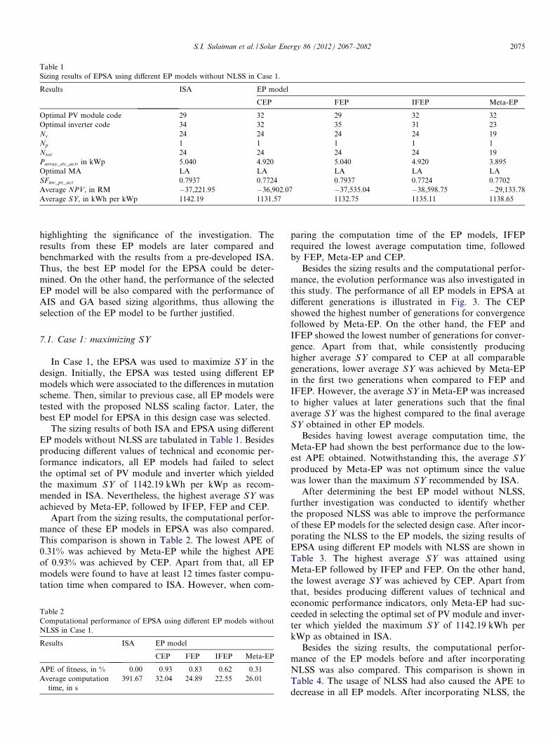
Table 1Sizing results of EPSA using different EP models without NLSS in Case 1.

Results ISA EP model

CEP FEP IFEP Meta-EP

Optimal PV module code 29 32 29 32 32Optimal inverter code 34 32 35 31 23Ns 24 24 24 24 19Np 1 1 1 1 1Ntot 24 24 24 24 19Parray_stc_act, in kWp 5.040 4.920 5.040 4.920 3.895Optimal MA LA LA LA LA LASFinv_pv_act 0.7937 0.7724 0.7937 0.7724 0.7702Average NPV, in RM �37,221.95 �36,902.07 �37,535.04 �38,598.75 �29,133.78Average SY, in kWh per kWp 1142.19 1131.57 1132.75 1135.11 1138.65


highlighting the significance of the investigation. Theresults from these EP models are later compared andbenchmarked with the results from a pre-developed ISA.Thus, the best EP model for the EPSA could be deter-mined. On the other hand, the performance of the selectedEP model will be also compared with the performance ofAIS and GA based sizing algorithms, thus allowing theselection of the EP model to be further justified.

7.1. Case 1: maximizing SY

In Case 1, the EPSA was used to maximize SY in thedesign. Initially, the EPSA was tested using different EPmodels which were associated to the differences in mutationscheme. Then, similar to previous case, all EP models weretested with the proposed NLSS scaling factor. Later, thebest EP model for EPSA in this design case was selected.

The sizing results of both ISA and EPSA using differentEP models without NLSS are tabulated in Table 1. Besidesproducing different values of technical and economic per-formance indicators, all EP models had failed to selectthe optimal set of PV module and inverter which yieldedthe maximum SY of 1142.19 kWh per kWp as recom-mended in ISA. Nevertheless, the highest average SY wasachieved by Meta-EP, followed by IFEP, FEP and CEP.

Apart from the sizing results, the computational perfor-mance of these EP models in EPSA was also compared.This comparison is shown in Table 2. The lowest APE of0.31% was achieved by Meta-EP while the highest APEof 0.93% was achieved by CEP. Apart from that, all EPmodels were found to have at least 12 times faster compu-tation time when compared to ISA. However, when com-

Table 2Computational performance of EPSA using different EP models withoutNLSS in Case 1.



APE of fitness, in % 0.00 0.93 0.83 0.62 0.31Average computation

time, in s391.67 32.04 24.89 22.55 26.01

paring the computation time of the EP models, IFEPrequired the lowest average computation time, followedby FEP, Meta-EP and CEP.

Besides the sizing results and the computational perfor-mance, the evolution performance was also investigated inthis study. The performance of all EP models in EPSA atdifferent generations is illustrated in Fig. 3. The CEPshowed the highest number of generations for convergencefollowed by Meta-EP. On the other hand, the FEP andIFEP showed the lowest number of generations for conver-gence. Apart from that, while consistently producinghigher average SY compared to CEP at all comparablegenerations, lower average SY was achieved by Meta-EPin the first two generations when compared to FEP andIFEP. However, the average SY in Meta-EP was increasedto higher values at later generations such that the finalaverage SY was the highest compared to the final averageSY obtained in other EP models.

Besides having lowest average computation time, theMeta-EP had shown the best performance due to the low-est APE obtained. Notwithstanding this, the average SY

produced by Meta-EP was not optimum since the valuewas lower than the maximum SY recommended by ISA.

After determining the best EP model without NLSS,further investigation was conducted to identify whetherthe proposed NLSS was able to improve the performanceof these EP models for the selected design case. After incor-porating the NLSS to the EP models, the sizing results ofEPSA using different EP models with NLSS are shown inTable 3. The highest average SY was attained usingMeta-EP followed by IFEP and FEP. On the other hand,the lowest average SY was achieved by CEP. Apart fromthat, besides producing different values of technical andeconomic performance indicators, only Meta-EP had suc-ceeded in selecting the optimal set of PV module and inver-ter which yielded the maximum SY of 1142.19 kWh perkWp as obtained in ISA.

Besides the sizing results, the computational perfor-mance of the EP models before and after incorporatingNLSS was also compared. This comparison is shown inTable 4. The usage of NLSS had also caused the APE todecrease in all EP models. After incorporating NLSS, the

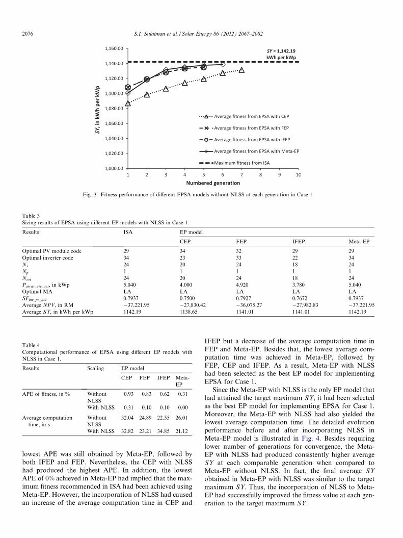
Fig. 3. Fitness performance of different EPSA models without NLSS at each generation in Case 1.

Table 3Sizing results of EPSA using different EP models with NLSS in Case 1.



Optimal PV module code 29 34 32 29 29Optimal inverter code 34 23 33 22 34Ns 24 20 24 18 24Np 1 1 1 1 1Ntot 24 20 24 18 24Parray_stc_act, in kWp 5.040 4.000 4.920 3.780 5.040Optimal MA LA LA LA LA LASFinv_pv_act 0.7937 0.7500 0.7927 0.7672 0.7937Average NPV, in RM �37,221.95 �27,830.42 �36,075.27 �27,982.83 �37,221.95Average SY, in kWh per kWp 1142.19 1138.65 1141.01 1141.01 1142.19

Table 4Computational performance of EPSA using different EP models withNLSS in Case 1.

Results Scaling EP model


APE of fitness, in % WithoutNLSS

0.93 0.83 0.62 0.31

With NLSS 0.31 0.10 0.10 0.00

Average computationtime, in s

WithoutNLSS

32.04 24.89 22.55 26.01

With NLSS 32.82 23.21 34.85 21.12


lowest APE was still obtained by Meta-EP, followed byboth IFEP and FEP. Nevertheless, the CEP with NLSShad produced the highest APE. In addition, the lowestAPE of 0% achieved in Meta-EP had implied that the max-imum fitness recommended in ISA had been achieved usingMeta-EP. However, the incorporation of NLSS had causedan increase of the average computation time in CEP and

IFEP but a decrease of the average computation time inFEP and Meta-EP. Besides that, the lowest average com-putation time was achieved in Meta-EP, followed byFEP, CEP and IFEP. As a result, Meta-EP with NLSShad been selected as the best EP model for implementingEPSA for Case 1.

Since the Meta-EP with NLSS is the only EP model thathad attained the target maximum SY, it had been selectedas the best EP model for implementing EPSA for Case 1.Moreover, the Meta-EP with NLSS had also yielded thelowest average computation time. The detailed evolutionperformance before and after incorporating NLSS inMeta-EP model is illustrated in Fig. 4. Besides requiringlower number of generations for convergence, the Meta-EP with NLSS had produced consistently higher averageSY at each comparable generation when compared toMeta-EP without NLSS. In fact, the final average SY

obtained in Meta-EP with NLSS was similar to the targetmaximum SY. Thus, the incorporation of NLSS to Meta-EP had successfully improved the fitness value at each gen-eration to the target maximum SY.

Fig. 4. Fitness performance of EPSA using Meta-EP with and without NLSS at each generation in Case 1.

Table 5Sizing results of EPSA using different EP models without NLSS in Case 2.



Optimal PV module code 39 26 26 3 19Optimal inverter code 8 7 7 8 8Ns 11 9 9 7 9Np 1 1 1 1 1Ntot 11 9 9 7 9Parray_stc_act, in kWp 1.936 1.935 1.935 1.890 1.980Optimal MA LA LA LA LA LASFinv_pv_act 0.7748 0.7752 0.7752 0.7937 0.7576Average SY, in kWh per kWp 1046.25 1085.41 1085.41 1075.03 1083.14Average NPV, in RM �11,181.99 �14,077.56 �14,077.56 �13,390.59 �12,243.48

Table 6Computational performance of EPSA using different EP models withoutNLSS in Case 2.



APE of fitness, in % 0.00 25.89 25.89 19.75 9.49Average computation

time, in s391.67 59.64 54.72 24.70 25.15


7.2. Case 2: maximizing NPV

In Case 2, the EPSA was used to maximize NPV in thedesign. Initially, the EPSA was tested using different EPmodels which are associated to the differences in mutationscheme. Then, similar to previous case, all EP models weretested with the proposed NLSS scaling factor. Later, thebest EP model for EPSA in this design case was selected.

The sizing results of both ISA and EPSA using differentEP models without NLSS are tabulated in Table 5. Apartfrom producing different values of technical and economicperformance indicators, all EP models had failed to selectthe optimal set of PV module and inverter which yieldedthe maximum NPV of �RM11, 181.99 as recommendedin ISA. Nevertheless, the highest average NPV wasachieved by Meta-EP, followed by IFEP. The lowest aver-age NPV was achieved in FEP and CEP.

Apart from the sizing results, the computational perfor-mance of these EP models without NLSS in EPSA was alsocompared. This comparison is shown in Table 6. The low-est APE of 9.49% was achieved by Meta-EP while the high-est APE of 25.89% was achieved by both CEP and FEP.

Apart from that, all EP models were found to have at least15 times faster computation time when compared to ISA.However, when comparing the computation time of theEP models, IFEP required the lowest average computationtime, followed by Meta-EP, FEP and CEP.

Besides the sizing results and the computational perfor-mance, the evolution performance was also investigated inthis study. The performance of all EP models in EPSA atdifferent generations is illustrated in Fig. 5. The Meta-EPrequired eight generations for convergence unlike othermodels which required only six generations for conver-gence. However, despite producing relatively lower average

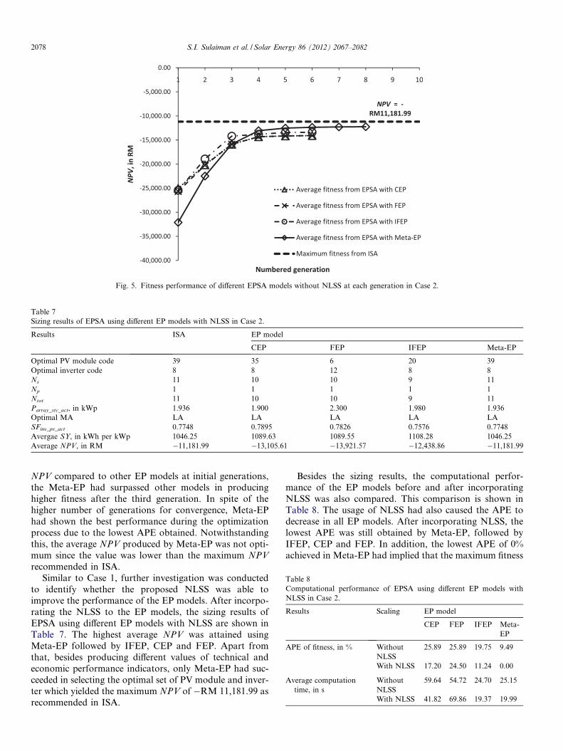
Fig. 5. Fitness performance of different EPSA models without NLSS at each generation in Case 2.

Table 7Sizing results of EPSA using different EP models with NLSS in Case 2.



Optimal PV module code 39 35 6 20 39Optimal inverter code 8 8 12 8 8Ns 11 10 10 9 11Np 1 1 1 1 1Ntot 11 10 10 9 11Parray_stc_act, in kWp 1.936 1.900 2.300 1.980 1.936Optimal MA LA LA LA LA LASFinv_pv_act 0.7748 0.7895 0.7826 0.7576 0.7748Avergae SY, in kWh per kWp 1046.25 1089.63 1089.55 1108.28 1046.25Average NPV, in RM �11,181.99 �13,105.61 �13,921.57 �12,438.86 �11,181.99

Table 8Computational performance of EPSA using different EP models withNLSS in Case 2.

Results Scaling EP model


APE of fitness, in % WithoutNLSS

25.89 25.89 19.75 9.49

With NLSS 17.20 24.50 11.24 0.00

Average computationtime, in s

WithoutNLSS

59.64 54.72 24.70 25.15

With NLSS 41.82 69.86 19.37 19.99


NPV compared to other EP models at initial generations,the Meta-EP had surpassed other models in producinghigher fitness after the third generation. In spite of thehigher number of generations for convergence, Meta-EPhad shown the best performance during the optimizationprocess due to the lowest APE obtained. Notwithstandingthis, the average NPV produced by Meta-EP was not opti-mum since the value was lower than the maximum NPV

recommended in ISA.Similar to Case 1, further investigation was conducted

to identify whether the proposed NLSS was able toimprove the performance of the EP models. After incorpo-rating the NLSS to the EP models, the sizing results ofEPSA using different EP models with NLSS are shown inTable 7. The highest average NPV was attained usingMeta-EP followed by IFEP, CEP and FEP. Apart fromthat, besides producing different values of technical andeconomic performance indicators, only Meta-EP had suc-ceeded in selecting the optimal set of PV module and inver-ter which yielded the maximum NPV of �RM 11,181.99 asrecommended in ISA.

Besides the sizing results, the computational perfor-mance of the EP models before and after incorporatingNLSS was also compared. This comparison is shown inTable 8. The usage of NLSS had also caused the APE todecrease in all EP models. After incorporating NLSS, thelowest APE was still obtained by Meta-EP, followed byIFEP, CEP and FEP. In addition, the lowest APE of 0%achieved in Meta-EP had implied that the maximum fitness

Fig. 6. Fitness performance of EPSA using Meta-EP with and without NLSS at each generation in Case 2.

Table 9Sizing results of different optimization methods in Case 1.

Results Optimization method

Meta-EP AIS GA

Optimal PV module code 29 32 29Optimal inverter code 34 21 33Ns 24 18 24Np 1 1 1Ntot 24 18 24Parray_stc_act, in kWp 5.040 3.690 5.040Optimal MA LA LA LASFinv_pv_act 0.7937 0.7588 0.7738Average SY, in kWh per kWp 1142.19 1120.95 1141.01

Table 10Computational performance of different optimization methods in Case 1.

Results ISA Optimization method

Meta-EPwith NLSS

AIS GA

APE of fitness, in % 0.00 0.00 1.86 0.10Average computation time, in s 391.67 21.12 104.31 57.58


recommended in ISA had been achieved. In addition, theincorporation of NLSS had caused the average computa-tion time in all EP models to decrease except for FEPwhich experienced an increase of computation time. Thelowest average computation time was achieved in IFEP fol-lowed by Meta-EP, CEP and FEP.

Although the lowest computation time was not achievedby Meta-EP with NLSS, the Meta-EP with NLSS had beenselected as the best EP model for implementing EPSA forCase 2 since it is the only EP model that had attained thetarget maximum NPV. The detailed evolution performancebefore and after incorporating NLSS in the Meta-EP withNLSS was illustrated in Fig. 6. Besides requiring lowernumber of generations for convergence, the Meta-EP withNLSS had also produced consistently higher average NPV

at each comparable generation when compared to Meta-EP without NLSS. In fact, the final average NPV obtainedin Meta-EP with NLSS was similar to the target maximumNPV. Thus, the incorporation of NLSS to Meta-EP hadsuccessfully improved the fitness value at each generationuntil the target maximum NPV was achieved.

7.3. Comparison with other optimization methods

As Meta-EP with NLSS had outperformed other EPmodels in all design cases, it was chosen as the optimalEP model for EPSA. Nevertheless, the performance ofthe proposed EPSA with Meta-EP using NLSS was furthercompared with the performance of GA-based sizing algo-rithm and AIS-based sizing algorithm to further justifiedthe selection of the optimization technique.

In Case 1, the results of the sizing process using selectedoptimization methods were tabulated in Table 9. Besidesproducing different sizing results, the highest average SYwas achieved in Meta-EP with NLSS, followed by GAand AIS.

In terms of computational performance in Case 1 asshown in Table 10, only Meta-EP with NLSS had pro-duced APE of 0% whereas both AIS and GA had producedhigher APE of 1.86% and 0.10% respectively. Besides that,the Meta-EP with NLSS had also yielded the lowest com-putation time, followed by GA and AIS. Meta-EP withNLSS was approximately 5 times faster than AIS and 3times faster than GA.

Apart from that, the performance of each optimizationmethod at different generations was illustrated in Fig. 7.Although the Meta-EP with NLSS had produced the low-est fitness value at the first two comparable generations

Fig. 7. Fitness performance of different optimization methods at each generation in Case 1.

Table 11Sizing results of different optimization methods in Case 2.

Results Optimization method

Meta-EP AIS GA

Optimal PV module code 39 26 30Optimal inverter code 8 7 8Ns 11 9 9Np 1 1 1Ntot 11 9 9Parray_stc_act, in kWp 1.936 1.935 1.890Optimal MA LA LA LASFinv_pv_act 0.7748 0.7752 0.7937SY, in kWh per kWp 1046.25 1085.41 1083.14Esys_exp, in kWh 2025.54 2100.26 2047.13Average NPV, in RM �11,181.99 �14,077.56 �11,930.20

Table 12Computational performance of different optimization methods in Case 2.

Results ISA Optimization method

Meta-EPwith NLSS

AIS GA

APE of fitness, in % 0.00 0.00 25.89 6.69Average computation time, in s 391.67 19.99 101.57 48.84

Fig. 8. Fitness performance of different optimiz


when compared to AIS and GA, it had outperformed AISin the next generation by producing higher fitness value butstill lower than the fitness produced by GA. Nevertheless,the subsequent generations required by Meta-EP withNLSS was used to improve the fitness value such that the

ation methods at each generation in Case 2.


final average SY was highest among the three methods andsimilar to the maximum SY obtained in ISA.

In Case 2, the results of the sizing process using selectedoptimization methods were tabulated in Table 11. Thehighest average NPV was achieved in both Meta-EP withNLSS and GA while the lowest average NPV was obtainedin AIS.

In terms of computational performance as shown inTable 12, only Meta-EP with NLSS and GA had producedAPE of 0% whereas both AIS and GA had producedhigher APE of 1.86% and 0.10% respectively. Besides that,the Meta-EP with NLSS had also yielded the lowest com-putation time, followed by GA and AIS. Meta-EP withNLSS was approximately 5 times faster than AIS and 3times faster than GA.

Apart from that, the performance of each optimizationmethod was illustrated in Fig. 8. Although the Meta-EPwith NLSS had produced the lowest fitness value at the ini-tial two comparable generations when compared to AISand GA, it had successfully outperformed AIS and GAin the fourth generation by producing higher fitness value.Then, the subsequent generation required by Meta-EP withNLSS was used to improve the fitness value such that thefinal average NPV was highest among the three methodsand similar to the maximum NPV obtained in ISA.

8. Conclusions

This paper presents an intelligent methodology towardssizing GCPV system when there are numerous sets of PVmodule and inverter that need to be considered in thedesign of the system. While the CSA presented a conven-tional method of sizing GCPV system based on a pre-deter-mined PV module and inverter, the ISA was developed asan extension of CSA using an iterative approach such thatall possible combinations of PV module and inverter weretested in the sizing process to identify an optimal designsolution. However, the proposed EPSA had presented anintelligent approach towards the sizing process such thatsimilar optimal design solution with the one obtained inISA could also be achieved with lower computation time.The EPSA utilized the PV module and inverter model asthe decision variables with an objective function of eitherto maximize the technical performance or to maximizethe economic performance of the system. These objectivefunctions were also reflected by the two design cases formu-lated in this study. Apart from that, the NLSS was alsofound to improve the performance of all EP modelsalthough only Meta-EP with NLSS had achieved the targetfitness value as produced by ISA in each design case. Inaddition, Meta-EP with NLSS had also outperformedother EP models in producing the lowest APE with com-petitively low computation time. On the other hand, whencompared with other optimization methods, the Meta-EPwith NLSS had outperformed AIS and GA in producingthe lowest APE and lowest computation time for everydesign case.

Acknowledgements

This work had been supported by the Fundamental Re-search Grant Scheme, Ministry of Higher Education,Malaysia (Grant: 600-RMI/ST/FRGS 5/3/Fst (81/2010).It is also partially supported by the Excellence Fund, Uni-versiti Teknologi MARA Malaysia (Ref: 600-RMI/ST/DANA 5/3/Dst (283/2009)).

References

Abdullah, N.R.H., Musirin, I., Othman, M.M., 2010. Transmission lossminimization using evolutionary programming considering UPFCinstallation cost. International Review of Electrical Engineering(June).

Abdullah, N.R.H., Musirin, I., Othman, M.M., 2010. Transmission lossminimization and UPFC installation cost using evolutionary compu-tation for improvement of voltage stability. In: Proceedings of the 14thInternational Middle East Power Systems Conference Cairo Univer-sity, Egypt, pp. 825–830.

Back, T., Rudolph, G., Schwefel, H.-P., 1993. Evolutionary programmingand evolution strategies: similarities and differences. In: SecondAnnual Conference on Evolutionary Programming, pp. 11–22.

Banos, R., Manzano-Agugliaro, F., Montoya, F.G., Gil, C., Alcayde, A.,Gomez, J., 2011. Optimization methods applied to renewable andsustainable energy: a review. Renewable and Sustainable EnergyReviews 15 (4), 1753–1766.

Chiong, R., Beng, O.K., 2007. A comparison between genetic algorithmsand evolutionary programming based on cutting stock problem.Engineering Letters 14 (1).

Chiong, R., Chang, Y.Y., Chai, P.C., Wong, A.L., 2008. A selectivemutation based evolutionary programming for solving cutting stockproblem without contiguity. In: IEEE Congress on EvolutionaryComputation. Hong Kong, 2008, pp. 1671–1677.

Damavandi, N., 2005. A hybrid evolutionary programming method forcircuit optimization. IEEE Transactions on Circuits and Systems 52(5), 902–910.

Dougherty, B.P., Fanney, A.H., Davis, M.W., 2005. Measured perfor-mance of building integrated photovoltaic panels – round 2. Journal ofSolar Energy Engineering 127 (3), 314–323.

Hoffmann, W., 2006. PV solar electricity industry: market growth andperspective. Solar Energy Materials & Solar Cells 90 (18–19), 3285–3311.

Installation of grid-connected photovoltaic (PV) system, 2010. MalaysianStandard MS 1837:2010.

Jayabarathi, T., Jayaprakash, K., Jeyakumar, D.N., Raghunathan, T.,2005. Evolutionary programming techniques for different kinds ofeconomic dispatch problems. Electric Power Systems Research 73 (2),169–176.

Kalogirou, S.A., December 2001. Artificial neural networks in renewableenergy applications: a review. Renewable and Sustainable EnergyReviews 5 (4), 373–401.

Kjaer, S.B., Pedersen, J.K., Blaabjerg, F., 2005. A review of single-phasegrid-connected inverters for photovoltaic modules. IEEE Transactionson Industry Applications 41 (5), 1292–1306.

Kornelakis, A., Koutroulis, E., 2009. Methodology for the designoptimisation and the economic analysis of grid-connected photovoltaicsystems. Renewable Power Generation, IET 3 (4), 476–492.

Kornelakis, A., Marinakis, Y., 2010. Contribution for optimal sizing ofgrid-connected PV-systems using PSO. Renewable Energy 35 (6),1333–1341.

Lewis, A., Abramson, D., Peachey, T., 2003. An evolutionary program-ming algorithm for automatic engineering design. In: Fifth Interna-tional Conference on Parallel Processing and Applied Mathematics,Czestochowa, Poland.


Mafigo, N., 2007. The Chinese silicon photovoltaic industry and market: acritical review of trends and outlook. Progress in Photovoltaics 15 (2),143–162.

Manoharan, P.S., Kannan, P.S., Ramanathan, V., 2009. A novel EPapproach for multi-area economic dispatch with multi-fuel options.Turkish Journal of Electrical Engineering and Computer Science 17(1), 1–19.

MBIPV, 2009. PV Industry Handbook. Pusat Tenaga Malaysia, Bangi.Mellit, A., Kalogirou, S.A., Hontoria, L., Shaari, S., 2009. Artificial

intelligence techniques for sizing photovoltaic systems: a review.Renewable and Sustainable Energy Reviews 13 (2), 406–419.

Omar, A.M., Shaari, S., 2009. Sizing verification of photovoltaic arrayand grid-connected inverter ratio for the Malaysian building integratedphotovoltaic project. International Journal of Low-Carbon Technol-ogies 4 (4), 254–257.

REN21, 2010. Renewables 2010 global status report. Paris.Salas, V., Olıas, E., 2009. Overview of the state of technique for PV

inverters used in low voltage grid-connected PV systems: invertersbelow 10 kW. Renewable and Sustainable Energy Reviews 13 (6–7),1541–1550.

Seng, L.Y., Lalchand, G., Lin, G.M.S., 2008. Economical, environmentaland technical analysis of building integrated photovoltaic systems inMalaysia. Energy Policy 36 (April), 2130–2142.

Shaari, S., Omar, A.M., Haris, A.H., Sulaiman, S.I., 2010. SolarPhotovoltaic Power: Designing Grid-connected Systems. KementerianTenaga, Teknologi Hijau dan Air, Putrajaya.

Shaari, S., Omar, A.M., Haris, A.H., Rahman, R.A., Sulaiman, S.I.,2010a. Solar Photovoltaic Power: Irradiation Data for Malaysia.Ministry of Energy, Green Technology & Water, Malaysia, Putrajaya.

Shaari, S., Omar, A.M., Haris, A.H., Sulaiman, S.I., 2010b. SolarPhotovoltaic Power: Fundamentals. Ministry of Energy, GreenTechnology and Water, Putrajaya.

Sinha, N., Chakrabarti, R., Chattopadhyay, K., 2004. Improved fastevolutionary program for economic load dispatch with non-smoothcost curves. IE (I) Journal 85 (September), 110–114.

Skoplaki, E., Palyvos, J.A., 2009. On the temperature dependence ofphotovoltaic module electrical performance. A review of efficiency/power correlations. Solar Energy 83 (5), 614–624.

Sulaiman, S.I., Rahman, T.K.A., Musirin, I., 2010. Design of grid-connected photovoltaic system using evolutionary programming. In:IEEE International Conference on Power and Energy (PECon), KualaLumpur, pp. 947–952.

Sulaiman, S.I., Rahman, T.K.A., Musirin, I., 2011. Artificial immunesystem for sizing grid-connected photovoltaic system. In: 5th Interna-tional Power Engineering and Optimization Conference (PEO-CO2011), Shah Alam, pp. 398–403.

Thomson, M., Infield, D.G., 2007. Impact on widespread photovoltaicspower generation on distributed systems. IET Renewable PowerGeneration 1 (1), 33–40.

Turcotte, D., Ross, M., Sheriff, F., 2001. Photovoltaic hybrid systemsizing and simulation tools: status and needs. In: PV Horizon:Workshop on Photovoltaic Hybrid Systems, pp. 1–10.

Verboomen, J., Hertem, D.V., Schavemaker, P.H., Kling, W.L., Belmans,R., 2006. Coordinated phase shifter control using meta-evolutionaryprogramming and evolutionary strategies. In: 3rd IEEE BeneluxYoung Researchers Symposium in Electrical Power Engineering,Ghent, Belgium, pp. 1–6.

Documents

An Intelligent Method for Sizing Optimization in Grid-connected Photovoltaic System