An integrated model for optimisation of production and quality costs

This article was downloaded by: [University of New Hampshire]On: 28 February 2013, At: 07:10Publisher: Taylor & FrancisInforma Ltd Registered in England and Wales Registered Number: 1072954 Registeredoffice: Mortimer House, 37-41 Mortimer Street, London W1T 3JH, UK

International Journal of ProductionResearchPublication details, including instructions for authors andsubscription information:http://www.tandfonline.com/loi/tprs20

An integrated model for optimisation ofproduction and quality costsWalid Abdul-Kader a , Ozhand Ganjavi b & Aim Solaiman ca Department of Industrial & Manufacturing Systems Engineering,University of Windsor, Ontario, Canadab School of Commerce, Laurentian University, Sudbury, Ontario,Canadac Weber Aircraft LLC, Gainesville, Houston, Texas, USAVersion of record first published: 01 Feb 2010.

To cite this article: Walid Abdul-Kader , Ozhand Ganjavi & Aim Solaiman (2010): An integratedmodel for optimisation of production and quality costs, International Journal of ProductionResearch, 48:24, 7357-7370

To link to this article: http://dx.doi.org/10.1080/00207540903382881

PLEASE SCROLL DOWN FOR ARTICLE

Full terms and conditions of use: http://www.tandfonline.com/page/terms-and-conditions

This article may be used for research, teaching, and private study purposes. Anysubstantial or systematic reproduction, redistribution, reselling, loan, sub-licensing,systematic supply, or distribution in any form to anyone is expressly forbidden.

The publisher does not give any warranty express or implied or make any representationthat the contents will be complete or accurate or up to date. The accuracy of anyinstructions, formulae, and drug doses should be independently verified with primarysources. The publisher shall not be liable for any loss, actions, claims, proceedings,demand, or costs or damages whatsoever or howsoever caused arising directly orindirectly in connection with or arising out of the use of this material.

http://www.tandfonline.com/loi/tprs20

http://dx.doi.org/10.1080/00207540903382881

http://www.tandfonline.com/page/terms-and-conditions

http://www.tandfonline.com/page/terms-and-conditions

International Journal of Production ResearchVol. 48, No. 24, 15 December 2010, 7357–7370

An integrated model for optimisation of production and quality costs

Walid Abdul-Kadera*, Ozhand Ganjavib and Aim Solaimanc

aDepartment of Industrial & Manufacturing Systems Engineering, University of Windsor,Ontario, Canada; bSchool of Commerce, Laurentian University, Sudbury, Ontario, Canada;

cWeber Aircraft LLC, Gainesville, Houston, Texas, USA

(Received 8 January 2009; final version received 30 September 2009)

Whether an industrial organisation is involved with production of new goods orengaged in reverse logistics to recycle used products, the items produced that donot meet specifications can cost the organisation in many different ways. Theadministrative expenses of handling returned items and the cost of reworking theitems that have failed in plant quality control or returned by customers can be ofconcern to the manufacturers. While these are measurable costs, there are othercosts such as loss of customers’ good will which are hard, if not impossible, toestimate. The model presented in this paper is aimed at optimising the measurablecost of reworking/scrapping the off-specification items as well as the cost ofadjusting manufacturing processes with the aim of reducing or eliminatingrejected pieces. The adjustment of process specification in relation to customerspecification is a strategy that can affect production and quality cost.Consideration for optimal production specification is one of the elements of themodel presented in this paper. In the proposed model, the direct cost of poorquality has been represented by a symmetrical truncated loss function. We haveconsidered investment to adjust the mean and variance of the process.A numerical example is presented to demonstrate how the model can work in areal-world setting.

Keywords: economic investment; quality; rework/scrap costs; process defects

1. Introduction

Some of the strategies utilised by manufacturing companies to compete in the market placeinclude attempts to lower cost and improve quality of their products. Waste reduction isan important element of minimising total cost of production (Raiman and Case 1990).Numerous journal articles, written in the recent past, on the subject of cost reduction focuson costs related to quality loss. In practice, the costs incurred in a production processinclude manufacturing costs, materials costs, quality loss cost, inspection costs, reworkcosts, and scrap costs. A search of the literature on this topic reveals that only a fewattempts have been made to combine manufacturing and quality related costs in anintegrated model. One of the focuses of this research work is on reduction of processvariance as well as bringing the process mean closer to its target. This element of the modelattempts to reduce the amount of products that are prone to extra costs of rework/repair.The cost function utilised in this part of our model will be Taguchi’s quadratic lossfunction.

*Corresponding author. Email: [email protected]

ISSN 0020–7543 print/ISSN 1366–588X online

� 2010 Taylor & Francis

DOI: 10.1080/00207540903382881

http://www.informaworld.com

Dow

nloa

ded

by [

Uni

vers

ity o

f N

ew H

amps

hire

] at

07:

10 2

8 Fe

brua

ry 2

013

The variation in quality characteristics of a product causes the reduction in its quality.Process deterioration is often the main cause of increased variation and henceoff-specification items. Off-specification items are often repaired and sent back to theoriginal station where defects are detected. At times a portion of off-specification items arediscarded rather than reworked (Chiu 2003). The rework/repair and discarding are not freeof costs. Taguchi et al. (1989) proposed a quadratic loss function to link the costs of poorquality to the level of quality characteristic or quality performance. In this context ‘qualityperformance’ means the closeness of a product’s functional performance to its desiredtarget value (Byrne and Taguchi 1986). The Taguchi quality cost function is overwhelmingin the reviewed literature as models presented by Chan et al. (2005), Chen (2006), Tsou(2006), and Peng et al. (2008) use this type of quality cost function. Another type of costfunction used in the literature is reflected normal.

The reflected normal loss function was proposed by Spiring (1993), and Spiring andYeung (1998) to capture quality loss costs. Kulkarni and Prybutok (2004) proposed amodification to the reflected normal loss function. This function was proposed as analternative to Taguchi’s loss function. Kulkarni (2008) presented a model for optimalinvestment for process variance reduction as well as optimal quality inspection and the lotsize. The quality loss function used in the model has a modified reflected normal form. It isinteresting to note that Kulkarni’s paper shows that as the variance of the processincreases the reflected normal approaches the Taguchi form of quality cost function. Thisis due to the fact that the convex part of the reflected normal curve falls outside of thetolerance limits when the variance is increased. We feel like most of the other researchersthat Taguchi’s quality cost function is adequate for the application. Taguchi’s functiondirectly links the quality characteristic to the internal and external failure costs. Theobjective of our quality improvement method is to minimise the sum of the internal andexternal failure costs.

Kapur and Wang (1987) proposed a short term solution to decrease the variance of theunits shipped to the customer by imposing specification limits on the process and truncateoff-specification through inspection. Their model does not attempt to reduce the processvariation; rather it inspects and removes the off-specification items to reduce the variationin the shipped items. Thus, they have added inspection cost and scrap cost in the lossfunction model. It is a general understanding that shifting the process mean is easier,in relative terms, compared to reducing the variance. Wen and Mergen (1999) establishedan optimal process mean by balancing the cost of not meeting the specification limits.Chen et al. (2002) modified Wen and Mergen’s model of optimal process mean byproviding a linear and quadratic asymmetrical quality loss function for items within andoutside of specification limits. Jeang and Yang (1992) consider tool wear as the mostimportant factor affecting machining accuracy. Their tool replacing model involves bothsymmetrical and asymmetrical quality loss functions. Vokurka and Davis (1996) presenteda case study in manufacturing scrap reduction through quality improvement. Cain andJanssen (1997) provided three asymmetrical loss functions for optimal process setting.Jeang (1997) utilised a response surface approach to minimise the total costs of toleranceand quality loss based on three cost estimation scenarios. Jeang (2001) presented a modelfor simultaneous optimisation of product and process design parameters. For situationswhere repairable defective items are reworked, Chiu and Chiu (2003) presented an EPQ(economic production quantity) model which behaves like the optimal lot sizing model butfor defective and scrap rates. Chiu (2003) considered the effect of the reworking ofdefective items with backlogging allowed.

7358 W. Abdul-Kader et al.

Dow

nloa

ded

by [

Uni

vers

ity o

f N

ew H

amps

hire

] at

07:

10 2

8 Fe

brua

ry 2

013

Boucher and Jafari (1991) utilised sampling plans to determine process targets. Pulakand Al-Sultan (1996) presented a model to find the optimal process target under rectifyinginspection plan. They added inspection plans to further expand the ideas of Boucher andJafari (1991). Chen (2006) proposed a model to determine optimum process mean andstandard deviation. This is a modified version of the work by Pulak and Al-Sultan (1996)for cases when there is rectifying inspection plan in place. The paper utilised Taguchi’s(1986) quadratic quality loss function in their model.

Chiu (2007) presented an economic manufacturing quantity (EMQ) model forscenarios when there are some random defective items produced and the defective itemsare subject to rework or scrapping. The model produces optimal levels of the lot-size andbacklogs to minimise expected overall costs. Sarker et al. (2008) presented an EPQinventory model for a multi-stage manufacturing system with rework process. Theyconsidered only two inventory policies. Cardenas-Barron (2009) provided correction andfurther expansion of the model presented by Sarker et al. (2008).

The above papers focus on reducing defective rates by optimising process settings.The following papers attempt to reduce defective rates by means of quality investment.Fine and Porteus (1989) allowed small, but frequent, quality investment overtime toreduce defective rates. Hong and Hayya (1993) presented a model relating processquality to process quality investment. The model contains expressions for processparameter changes in terms of quality investment. Ouyang and Chang (2000)investigated the effect of quality improvement on modified lot size reorder pointmodels involving variable lead-time and partial backorders. Their model considers animperfect production process with the provision of an investment option to improvethe process quality. Ouyang et al. (2002) presented the options of investing in processquality improvement and in setup cost reduction. The lead-time can be shortened foran extra crashing cost.

A significant development in this field, in the form of a financial cost model for qualityinvestment, has been presented by Chen and Tsou (2003). Their notable contributioninvolves expressions for the mean and variance of the process as a function of investment.This is the focus of our research as well. Similar expressions have been presented in otherpapers, but they are in most part based on the proposed cost models by Hong and Hayya(1993), and Ganeshan et al. (2001).

Affisco et al. (2002) presented a lot size model with consideration to invest in qualityimprovement and setup cost reduction by a vendor. They investigated the impact of such ameasure on system-wide cost reduction in a supply chain. The quality investment functionutilised in this paper sets the level of quality measures as an exponential function of thelevel of quality investment. Liu and Cetinkaya (2007) proposed a modification to theinvestment function used by Affisco et al. (2002). Their function not only includes a onetime investment but also considers additional annual improvement expenditure. Theystated that this modification in investment function drastically changes the resultsobtained by Affisco et al. (2002).

Chan et al. (2005) presented a model for joint determination of quality investment levelto reduce process variance, and optimal lot size. They used Taguchi’s loss function. Tsouand Chen (2005) studied a dynamic model for a defective production system withmistake-proofing (poka-yoke). They stated that mistake-proofing activities have an effecton the cost of a production system, and the effect depends on the cost of mistake-proofingand the probability of the process going out of control. Tsou (2006) presented a model toexplore the effects of investing in process improvements as well as setting the lot size.

International Journal of Production Research 7359

Dow

nloa

ded

by [

Uni

vers

ity o

f N

ew H

amps

hire

] at

07:

10 2

8 Fe

brua

ry 2

013

The quality characteristic is assumed to be normally distributed and the loss function usedis the Taguchi’s truncated loss function.

Peng et al. (2008) proposed a model that considers the present value of the cost ofdeteriorating quality with usage to optimise quality level of the product off the productionline. The model considers Taguchi loss function but it is extended to a multivariate lossfunction. Liao et al. (2009) provided a model for expected cost by integrating maintenanceand production programmes for a production system that is deteriorating and themaintenance is not perfectly performed.

The existing literature, as discussed above, models the interaction between theeconomics of production and process quality improvement. Current research focuses, in alarge part, on economic lot-size models generated by quality improvements. The economiclot-scheduling models can contribute to the joint decision of economic production andquality investment, but they do not segregate the financial returns of quality investmentsto a company. This shortcoming limits the practical use of these cost models and hencepresents an opportunity for further research. Moreover, manufacturing cost and reworkcost are also related to process tolerance (Chase and Greenwood 1988), which is notincluded in earlier cost models.

In this paper, three significant contributions are made to the field of study. First, wedevelop a total costs model to determine the optimal process tolerance limits. Second, weintroduce our investment model to determine the amount of quality investment necessaryin order to economically correct a defective process resulting in minimum cost ofproduction. Third, we combine the above two models into an integrated cost model thatcan help the joint decision on the level of investment and with tolerance limits in order toachieve optimal process settings. The savings will be realised by the reduction of rework/scrap costs. The literature survey, presented earlier, indicates that this type of modellingapproach has not been tried in the field of defective process improvement and economicsof quality investment.

The remainder of this paper is organised as follows: Section 2 discusses the integratedcost model and its two sub-models. In Section 3, the tolerance model which is the firstsub-model of the integrated cost model is discussed. Quality investment model, the secondsub-model of the integrated cost model is described in Section 4. Section 5 is dedicated to acase study showing the modelling steps and analytical results in order to verify ourproposed model. Finally, the conclusion of this paper is provided in Section 6.

2. The integrated cost model

The production system under study is a serial production line producing discrete products.The manufacturing process can produce some nonconforming products due to processdefects. The reworking of defective products starts immediately after the regularproduction ends. There is a cost associated with further processing of defective products.A portion of the repaired items is rejected as scrap. The mean and variance of the processcan be modified at a cost. The cost of variance reduction is, generally, much bigger thanthe cost of mean adjustment. Product specification is a decision parameter, and there is acost associated with looser specification.

The total cost would be affected by decisions regarding process modification andchanges in specification. The purpose of the integrated cost model is to determine the bestquality specification and the best quality investment level, mostly for variance reduction,


Dow

nloa

ded

by [

Uni

vers

ity o

f N

ew H

amps

hire

] at

07:

10 2

8 Fe

brua

ry 2

013

to achieve the minimum expected total cost per unit of the product. The ‘integrated costmodel’ is composed of two sub-models, the ‘tolerance model’ and the ‘investment model’.The tolerance model determines the optimal tolerance limits to minimise cost. Theinvestment model determines the optimal quality investment necessary in order to correcta defective process with minimum cost of production. The integrated cost model combinesthe above two models into a single model that can facilitate joint decisions on toleranceand investment levels.

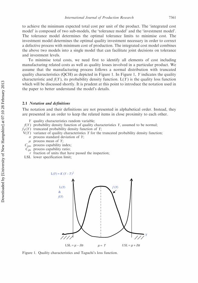
To minimise total costs, we need first to identify all elements of cost includingmanufacturing related costs as well as quality losses involved in a particular product. Weassume that the manufacturing process follows a normal distribution with truncatedquality characteristics (QCH) as depicted in Figure 1. In Figure 1, Y indicates the qualitycharacteristic and f(Y ), its probability density function. L(Y ) is the quality loss functionwhich will be discussed shortly. It is prudent at this point to introduce the notation used inthe paper to better understand the model’s details.

2.1 Notation and definitions

The notation and their definitions are not presented in alphabetical order. Instead, theyare presented in an order to keep the related items in close proximity to each other.

Y quality characteristics random variable;f(Y ) probability density function of quality characteristics Y, assumed to be normal;

fT(Y ) truncated probability density function of Y;V(Y ) variance of quality characteristics Y for the truncated probability density function;

� process standard deviation of Y;� process mean of Y;

Cpm process capability index;Cpk process capability ratio;

r fraction of units that have passed the inspection;LSL lower specification limit;

L(Y) = K (Y – T )2

L(Y) f (Y)

&

f(Y)

Y

LSL = m − Zσ USL = m + Zσm = T

Figure 1. Quality characteristics and Taguchi’s loss function.


Dow

nloa

ded

by [

Uni

vers

ity o

f N

ew H

amps

hire

] at

07:

10 2

8 Fe

brua

ry 2

013

USL upper specification limit;t process tolerance of Y which is ðUSL� LSLÞ=2;Z ratio of tolerance to � (a constant) ¼ t=�;

� ð�Þ probability density function of standard normal variable;�ð�Þ cumulative probability of standard normal variable;

I cost of quality investment;L(Y ) quality loss function; in our case it is KðY� T Þ2;

T target value of Y, for properly adjusted process T ¼ �;K cost coefficient of quality loss;Ic inspection cost/unit;

Mc manufacturing cost/unit;Pc part and material cost/unit;Rc rework cost/unit;Sc scrap cost/unit;

C(Y ) total cost as a function of quality characteristic Y;TC expected total cost per item. TC ¼ E[C(Y )];�I process mean associated with quality investment I;�I process standard deviation associated with quality investment I;�2M maximum (before investment) level of the process variance;

�2L minimum achievable level of the process variance;�0 initial value of the process mean at the decision time;�T target value of the process mean;� investment function parameter for process variance;� investment function parameter for process mean.

As depicted in Figure 1, based on truncated distribution we can have three scenarios:

(1) When the dimension of part is falling within the specification limits;(2) When the dimension of part is above the specification upper limit;(3) When the dimension of part is below the specification lower limit.

The expected total cost, TC, can be written as:

TC ¼ E CðY Þ½ �

¼ E C LSL � Y � USLð Þ þ C Y4USLð Þ þ C Y5LSLð Þ½ �: ð1Þ

There are generally four scenarios regarding the treatment of the off-specification

products:

(1) Off-specification items on both tails of the distribution are discarded;(2) Off-specification items on both tails of the distribution are reworked;(3) Off-specification on the high end is discarded and on the low end is reworked;(4) Off-specification on the low end is discarded and on the high end is reworked.

Procedures to produce expected costs for these four scenarios are similar with some

differences in total expected cost for each scenario. We shall develop the cost for scenario

number (4), which is the appropriate case for our example presented in Section 5. Hence

the expression for C(Y ) would be:

CðY Þ ¼Pc þMc þ KðY� T Þ2 þ Ic, for �� Z� � Y � �þ Z�Pc þMc þ Rc þ Ic, for �þ Z�5Y2Pc þ 2Mc þ Sc þ Ic, for Y5�� Z�

8<: : ð2Þ

The last two lines in Equation (2) indicate that when Y is too large there will be a cost

of rework and when Y is too small, the part must be scrapped and a new part must be built

to replace it. There is always the argument that a portion of rework or replacement of the


Dow

nloa

ded

by [

Uni

vers

ity o

f N

ew H

amps

hire

] at

07:

10 2

8 Fe

brua

ry 2

013

off-specification items may also be off as well. This amount is so small that for practicalreasons we consider it to be zero, e.g., if 5% of items are above USL and will receiverework, and if 5% of the rework turns out to be above USL this amounts to 0.25% of theoriginal batch. For simplicity of modelling and because these quantities are small, weconsider them to be zero. We assume all the reworks and all the replacement for discardeditems meet the target value and would not result in any additional extra cost of quality.The expression KðY� T Þ2 in the first line of the cost function is Taguchi’s quality lossfunction.

2.2 Methodology for integrating costs

As indicated earlier, there are two sub-models for our integrated cost model, the tolerancemodel and the investment model. These sub-models are utilised in a sequence of twophases. Phase-I starts with a known defective process. We identify the process parametersand measure their respective values. Then, we plug those parameters into the tolerancemodel to determine the optimum tolerance limits. The output of the tolerance modelbecomes an input for the investment model.

In Phase-II, the new levels of mean and variance are unknown and are a function of theinvestment level. We set the specification limits, as determined by the tolerance model, andplug them into the quality investment model. The solution of the investment modelproduces the optimal process mean and standard deviation to minimise the productioncost. The investment cost is spent to improve the performance of the process by decreasingthe variance and bringing the mean closer to its target. This action will result in a decreaseof rework/scrap costs.

3. Tolerance model

The rest of this section presents the tolerance model as follows:

TC ¼ ðIc þMc þ PcÞ þ ðMc þ Pc þ Rc þ ScÞ g1 þ K�2g2,

where

g1 ¼ 1��ðZÞð Þ and g2 ¼ 1�2Z� ðZÞ

2�ðZÞ � 1

� �:

It is worth noting that the variance of the process �2 is a given parameter of the model.The above model is used to determine the optimal level of Z to produce the minimum totalexpected cost. The value of Z determines the LSL and the USL. Let us now demonstratehow this model is derived.

As we stated in the paragraph after Equation (2), the Taguchi quality loss function forY values between the specification limits is L(Y ) ¼KðY� T Þ2. The best case scenario iswhen the process mean is cantered at its target, that is � ¼ T. In such a case we have:

E½LðYÞ� ¼ EKðY� T Þ2

¼ KEðY� TÞ2

¼ KEðY� �Þ2

¼ KVðY Þ: ð3Þ


Dow

nloa

ded

by [

Uni

vers

ity o

f N

ew H

amps

hire

] at

07:

10 2

8 Fe

brua

ry 2

013

where V(Y ) is the variance of the truncated probability density function of Y, which isdifferent from �2, the variance of Y before truncation. Equation (3) reveals that lowervalues of variance V(Y ) are associated with lower expected quality loss. The variance V(Y )can be lowered by lowering �2 as well as by tightening the specification limits.

To find an expression for V(Y ) we need to know the:

. Variance of the process distribution;

. Relationship between process tolerances and the truncated variance.

Let us begin with the relationship between process tolerances and process variability.One way to address this relationship is to use the process capability index, which is a betterindicator of centring:

Cpm ¼USL� LSL

6�, ð4Þ

where � is the square root of the expected squared deviation from target T. T equalsðUSLþ LSLÞ=2, and USL and LSL are the upper and lower specification limitsrespectively.

For the general case when T and � are different, we have:

�2 ¼ E½ðY� T Þ2�

¼ E½ðY� �Þ2� þ ð�� T Þ2

¼ �2 þ ð�� T Þ2:

For the case of � ¼ T, we have �2 ¼ �2. In Equation (4), we replace the term(USL�LSL) with 2t and � with �, so that:

Cpm ¼t

3�: ð5Þ

If Z represents the ratio of t over � (i.e., Z ¼ t=�), Z ¼ 3Cpm. Here Z would be theindicator for process capability.

So far, we have the relationship between tolerance, t, and process standard deviation,�. Next, we discuss the variance of truncated distribution.

After a total inspection, the out-of-specification products are removed. The probabilitydensity function of those items that have passed the screening (acceptable items) is givenby dividing the probability density function of Y by, r, the proportion of acceptable items(Taguchi et al. 1989). Let fTðY Þ be the probability density function for the truncatedrandom variable Y. Then we have:

fTðY Þ ¼1

r

1

�ffiffiffiffiffiffi2�p e �

ðY��Þ2

2�2

� �:

where r ¼ 2�ðZÞ � 1 is the area under the normal curve bounded by (�� Z�) and(�þ Z�) for positive values of Z; and �ðZÞ is the cumulative distribution function for thestandard normal variable. Therefore, the variance of the passed items, V(Y ), would be:

VðY Þ ¼

Z �þZ�

��Z�

ðY� T Þ2fTðY ÞdY

¼

Z �þZ�

��Z�

ðY� T Þ21

r

1


ðY��Þ2

2�2

� �dY:


Dow

nloa

ded

by [

Uni

vers

ity o

f N

ew H

amps

hire

] at

07:

10 2

8 Fe

brua

ry 2

013

For the case of T ¼ �, we obtain:

VðY Þ ¼

Z �þZ�

��Z�

ðY� �Þ21

r

1


ðY��Þ2

2�2

� �dY: ð6Þ

Performing integration by parts, V(Y ) is obtained as shown in Equation (7) (Kapur and

Wang 1987):

VðY Þ ¼ �2 1�2Z�ðZÞ

2�ðZÞ � 1

� �: ð7Þ

Equation (7) is the expression of the variance of the truncated distribution in terms of the

process variance �2 and process capability represented by Z, which in turn is a function of

the tolerance.Expanding the expression for expected cost developed in Equation (2), we obtain:

EðCðY ÞÞ ¼

Z �þz�

��z�

½Pc þMc þ KðY� T Þ2 þ Ic� f ðY ÞdY

þ ðPc þMc þ Ic þ RcÞ

Z 1�þz�

f ðY ÞdY

þ ð2Pc þ 2Mc þ Sc þ IcÞ

Z ��z�

�1

f ðY ÞdY:

By completing the process of integration in the above expression, we obtain the following

model:

EðCðY ÞÞ ¼ ðMc þ Pc þ Rc þ ScÞ½1��ðZÞ� þ Ic þMc þ Pc þ K�2 1�2z�ðzÞ

2�ðzÞ � 1

� �ð8Þ

This can be simplified into the following model:

TC ¼ EðCðY ÞÞ

¼ ðIc þMc þ PcÞ þ ðMc þ Pc þ Rc þ ScÞ g1 þ K�2g2, ð9Þ

where,

g1 ¼ ½1��ðzÞ� and g2 ¼ 1�2z�ðzÞ

2�ðzÞ � 1

� �:

Equation (9) is our tolerance model. The only unknown in this model is ‘Z’. Throughminimisation of TC, we can obtain an optimum value of Z. Since t ¼ Z�, the optimal

tolerance limit will be computed easily. In the following sections, we present the steps

involved in the formation of the quality investment model.

4. Quality investment model

Quality deterioration due to equipment wear is a common phenomenon in any production

process. Corrective actions and maintenance can ameliorate the situation or evencompletely eliminate such adverse effects. The distinct feature of our research is the study

of economic justification of quality investment in deteriorated processes.


Dow

nloa

ded

by [

Uni

vers

ity o

f N

ew H

amps

hire

] at

07:

10 2

8 Fe

brua

ry 2

013

As it was stated earlier, the output of our tolerance model will become an input for theinvestment model. The optimal tolerance limit obtained from the tolerance model will beutilised in the investment model to establish the best mean and variance for the process,

and hence the level of investment that can produce such an outcome. The uniqueness ofthis approach, compared to the other published work, is the fact that the model takes themean and variance of the process as decision variables. As the wear on equipment causesshifts in the mean and increases in the variance, considering them as decision variables,and subjecting them to modification, while maintaining a certain tolerance, seems to belogical. In the course of developing our model, the new levels of mean and variance will besubstituted with the level of capital needed to obtain them.

4.1 Working assumptions

To develop the investment model, the following four working assumptions havebeen made:

(1) The variables in the model are Y, the quality characteristic, and I, the qualityinvestment.

(2) Both the mean and standard deviation are functions of quality investment. Inpractice a finite number of investment levels are considered; hence, there would bea finite number of values for the mean and standard deviation of the process after

an investment is made. For instance, for investment Ii, the process parameterswould be �Ii and �Ii . With this view, we consider, �I and �I to be the mean andstandard deviation associated with quality investment I. The values of �I and �Iare defined as per Chen and Tsou (2003) to be:

�2I ¼ �2L þ ð�

2M � �

2LÞeð��I Þ, �4 0

�2I ¼ �

2T þ ð�

20 � �

2TÞeð��I Þ, �4 0,

where, �2M is the maximum (before investment) level of the variance and �2L is theminimum achievable level of the variance. Also, �0 is the initial value of the meanat the decision time, and �T is the mean’s target value. Since, the initial and targetvalues are known, the parameters � and � could be found through regressionanalysis of historical data.

(3) The process density function will have one more parameter I, the investment levelas shown below:

f ðY, I Þ ¼1

�Iffiffiffiffiffiffi2�p e

�ðY��I Þ

2

2�2I :

(4) Poor quality cost is the integral of Taguchi loss function, L(Y ), times the density

function, from LSL to USL as shown below:

Poor quality cost=unit ¼

Z USL

LSL

KðY� T Þ2 � f ðY, I ÞdY:


Dow

nloa

ded

by [

Uni

vers

ity o

f N

ew H

amps

hire

] at

07:

10 2

8 Fe

brua

ry 2

013

4.2 Model derivation

Considering the above working assumptions, and adding the cost of investment to theexpected cost model, we arrive at:

EðCðY, I ÞÞ ¼ ðPc þMc þ Ic þ RcÞ

Z 1USL

f ðY, I ÞdY

þ ð2Pc þ 2Mc þ Ic þ ScÞ

Z LSL

�1

f ðY, I ÞdY

þ

Z USL

LSL

½Pc þMc þ KðY� T Þ2 þ Ic� f ðY, I ÞdYþ I:

Due to symmetry the first two integrals are equal, hence we can further simplify ourmodel of expected cost and attempt to minimise it subject to two simple constraints,and we arrive at our investment model:

Minimise:

TCðY, I Þ ¼ ð3Pc þ 3Mc þ 2Ic þ Rc þ ScÞ

Z LSL

�1

f ðY, I ÞdY

þ ðPc þ Ic þMcÞ

Z USL

LSL

f ðY, I ÞdY

þ

Z USL

LSL

LðY Þ � f ðY, I ÞdY þ I:

Subject to:

Y � 0 and I � 0:

The aim of this model is to determine the optimal level of investment to minimise thetotal expected cost.

In the next section, a numerical example is presented to demonstrate how the twomodels work together.

5. Numerical example

The manufacturing facility used as an example belongs to a seat manufacturing company,which is a prime supplier of car seats for one of the big three car companies. The facility islocated on the outskirts of the city of Windsor in Ontario, Canada. In a two-shiftoperation, more than 500 car seats are produced. The operations are performed indifferent workstations of the facility and parts and semi-assemblies are carried to properlocations on pallets. The main activities involved in making a car seat include: back build(frame) for the seat and the headrest; foaming of the seat and head rest; skinning of thefoamed frames; coupling of the headrest to the seat; and some functional tests. The studywas conducted by one of the authors before the 2008–2009 meltdown of the auto industry.The operation used as an example in this paper includes the following information. Carseats in lots of 280 seats per shift and operates two shifts per day. The Production Managerhas identified a dimensional problem in the base frame assembly, where a large number ofseats are taken back to the rework area because of a failure in the functional test.The Production Manager wants to determine how much investment is necessary in orderto address the problem. The input parameters of this situation are given in Table 1.


Dow

nloa

ded

by [

Uni

vers

ity o

f N

ew H

amps

hire

] at

07:

10 2

8 Fe

brua

ry 2

013

5.1 Solution procedure

Plugging the input parameters into the tolerance model and solving it we obtain the valuespresented in Table 2. Tolerance t¼Z� ¼ 3.15� 0.66¼ 2.07mm. Thus, for T¼ 402mm,the optimal specification would be: LSL¼ 399.93mm and USL¼ 404.07mm.

Utilising the specification obtained from the tolerance model, plus T¼ 402mm,�¼ 0.66mm into the investment model and solving it, usingMaple 10 software, we arrive atthe optimal value of the required investment and process parameters �I and �I as shownin Table 3.

This means that an investment of $663.38 should adjust the mean to 402mm and thestandard deviation to 0.1986mm. This results in an average cost per seat of $61.38. Thelower cost per seat has been achieved mostly through reduction in reworks/scraps.

6. Conclusions

In this paper, we have presented an integrated cost model composed of a tolerance modeland an investment model. Our primary objective has been to study the interactionsbetween cost of production and process quality to develop a tool for deciding how toreduce the extra costs of rework/scrap. With this view, we have developed the cost modelsbased on the relevant manufacturing costs and Taguchi’s model of quality loss. This modelcan be applied in any manufacturing process where excess variability in qualitycharacteristics causes defects and process wastes. The primary contribution of the

Table 1. The input parameters of the car seat problem.

Target process mean T 402mmCurrent process mean � 402.86mmCurrent standard deviation � 0.66Taguchi loss constant K $25.00Variance curve constant � 0.00362Mean curve constant � 0.0105Manufacturing cost Mc $11.03Part cost Pc $45.00Rework cost Rc $11.03Scrap cost Sc $12.00Inspection cost Ic $2.00

Table 2. The outputs of the tolerance model.

Optimal Z 3.15Optimal tolerance t 2.07mmLower specification limit LSL 399.93Upper specification limit USL 404.07

Table 3. The outputs of the investment model.

Optimal investment I $663.38Optimal mean �I 402.0mmOptimal standard deviation �I 0.1986Total costs per item, TC $61.38


Dow

nloa

ded

by [

Uni

vers

ity o

f N

ew H

amps

hire

] at

07:

10 2

8 Fe

brua

ry 2

013

integrated model is the fact that the production manager can utilise the model to takeoptimal investment decisions to correct a defective process. Comparison can also be madebetween the expected unit costs before and after the process modification. In summary, themost important contribution of this paper is the synthesis of the existing knowledge into ausable tool for decision making purposes. Future research could focus on two areas: first,on how the process parameters including optimal investment change if the process followsdistributions other than normal distribution; and second, on how the model can beexpanded to encompass scenarios with multiple quality characteristics.

Acknowledgements

The authors would like to acknowledge anonymous referees for the helpful comments regarding thefirst draft of the paper. They would like also to acknowledge the financial support of the NaturalSciences and Engineering Council of Canada with regard to this project.

References

Affisco, J.F., Paknejad, M.J., and Nasri, F., 2002. Quality improvement and setup reduction in the

joint economic lot size model. European Journal of Operational Research, 142 (3), 497–508.Boucher, T.O. and Jafari, M.A., 1991. The optimum target value for single filling operations with

quality sampling plans. Journal of Quality Technology, 23 (1), 44–47.Byrne, D.M. and Taguchi, S., 1986. The Taguchi approach to parameter design. ASQC Quality

Congress Transactions, Anaheim, CA, 177, 168–173.Cain, M. and Janssen, C., 1997. Target selection in process control under asymmetric costs. Journal

of Quality Technology, 29 (4), 464–468.

Cardenas-Barron, L.E., 2009. On optimal batch sizing in a multi-stage production system with

rework consideration. European Journal of Operational Research, 196 (3), 1238–1244.Chan, W.M., Ibrahim, R.N., and Lochert, P.B., 2005. Economic production quantity and process

quality: a multivariate approach. International Journal of Quality & Reliability Management,

22 (6), 591–606.

Chase, K.W. and Greenwood, W.H., 1988. Design issues in mechanical tolerance analysis.

Manufacturing Review, 1 (1), 50–67.Chen, C.H., Chou, C.Y., and Huang, K.W., 2002. Determining the optimum process mean under

quality loss function. International Journal of Advanced Manufacturing Technology, 20 (8),

598–602.

Chen, C.H., 2006. The modified Pulak and Al-Sultan’s model for determining the optimum process

parameters. Communications in Statistics – Theory and Methods, 35 (10), 1767–1778.Chen, J.-M. and Tsou, J.-C., 2003. An optimal design for process quality improvement: modeling

and application. Production Planning and Control, 14 (7), 603–612.Chiu, S.W. and Chiu, Y.P., 2003. An economic production quantity model with the rework process

of repairable defective items. Journal of Information & Optimization Sciences, 24 (3), 569–582.Chiu, S.W., 2007. Optimal replenishment policy for imperfect quality EMQ model with rework and

backlogging. Applied Stochastic Models in Business and Industry, 23 (2), 165–178.Chiu, Y.P., 2003. Determining the optimal lot size for the finite production model with random

defective rate, the rework process, and backlogging. Engineering Optimization, 35 (4), 427–437.

Fine, C.H. and Porteus, E.L., 1989. Dynamic process improvement. Operations Research, 37 (4),

580–591.Ganeshan, R., Kulkarni, S., and Boone, T., 2001. Production economics and process quality: a

Taguchi perspective. International Journal of Production Economics, 71 (1–3), 343–351.


Dow

nloa

ded

by [

Uni

vers

ity o

f N

ew H

amps

hire

] at

07:

10 2

8 Fe

brua

ry 2

013

Hong, J.D. and Hayya, J.C., 1993. Process quality improvement and setup reduction. InternationalJournal of Production Research, 31 (11), 2693–2708.

Jeang, A. and Yang, K., 1992. Optimum tool replacement with nondecreasing tool wear.International Journal of Production Research, 30 (2), 299–314.

Jeang, A., 1997. An approach of tolerance design for quality improvement and cost reduction.International Journal of Production Research, 35 (5), 1193–1211.

Jeang, A., 2001. Combined parameter and tolerance design optimization with quality and cost.

International Journal of Production Research, 39 (5), 923–952.Kapur, K.C. and Wang, C.J., 1987. Economic design of specification based on Taguchi’s concept of

quality loss function. Quality: design, planning, and control. R.E. Devor and S.G. Kapoor, eds.

The Winter annual meeting of the American Society of Mechanical Engineers, Boston, 23–26.Kulkarni, S. and Prybutok, V., 2004. Process investment and loss functions: models and analysis.

European Journal of Operational Research, 157 (1), 120–129.

Kulkarni, S.S., 2008. Loss-based quality costs and inventory planning: general models and insights.European Journal of Operational Research, 188 (2), 428–449.

Liao, G.L., Chen, Y.H., and Sheu, S.H., 2009. Optimal economic production quantity policy forimperfect process with imperfect repair and maintenance. European Journal of Operational

Research, 195 (2), 348–357.Liu, X. and Cetinkaya, S., 2007. A note on ‘quality improvement and setup reduction in the joint

economic lot size model’. European Journal of Operational Research, 182 (1), 194–204.

Ouyang, L.-Y. and Chang, H.C., 2000. Impact of investing in quality improvement on (Q, r, L) modelinvolving the imperfect production process. Production Planning & Control, 11 (6), 598–607.

Ouyang, L.-Y., Chen, C.-K., and Chang, H.C., 2002. Quality improvement, setup cost and lead-time

reductions in lot size recorder point models with an imperfect production process. Computers& Operations Research, 29 (12), 1701–1717.

Peng, H.P., et al., 2008. Optimal tolerance design for products with correlated characteristics byconsidering the present worth of quality loss. International Journal of Advanced Manufacturing

Technology, 39 (1–2), 1–8.Pulak, M.F.S. and Al-Sultan, K.S., 1996. The optimum targeting for a single filling operation with

rectifying inspection. Omega – The International Journal of Management Science, 24 (6),

727–733.Raiman, L.B. and Case, K.E., 1990. Monitoring continuous improvement using the Taguchi loss

function. In: Proceedings of the international industrial engineering conference, 20–23 May,

San Francisco, California, 391–395.Sarker, B.R., Jamal, A.M.M., andMondal, S., 2008. Optimal batch sizing in a multi-stage production

system with rework consideration. European Journal of Operational Research, 184 (3), 915–929.

Spiring, F.A., 1993. The reflected normal loss function. The Canadian Journal of Statistics, 21 (3),321–330.

Spiring, F.A. and Yeung, A.S., 1998. A general class of loss functions with industrial applications.Journal of Quality Technology, 30 (2), 152–160.

Taguchi, G., 1986. Introduction to quality engineering. Asian Productivity Organization (distributedby American Supplier Institute Inc., Dearborn, MI).

Taguchi, G., Elsayed, A., and Hsiang, T.C., 1989. Quality engineering in production systems. Book

series: industrial engineering and management science. New York: McGraw Hill.Tsou, J.-C. and Chen, J.-M., 2005. Dynamic model for a defective production system with poka-

yoke. The Journal of the Operational Research Society, 56 (7), 799–803.

Tsou, J.C., 2006. Decision-making on quality investment in a dynamic lot sizing production system.International Journal of Systems Science, 37 (7), 463–475.

Vokurka, R.I and Davis, R.A., 1996. Quality improvement implementation: a case study inmanufacturing scrap reduction. Production and Inventory Management Journal, 37 (3), 63–68.

Wen, D. and Mergen, A.E., 1999. Running a process with poor capability. Quality Engineering,11 (4), 505–509.


Dow

nloa

ded

by [

Uni

vers

ity o

f N

ew H

amps

hire

] at

07:

10 2

8 Fe

brua

ry 2

013

Documents

An integrated model for optimisation of production and quality costs