An instrumented saxophone mouthpiece and its use to understand

HAL Id: hal-00445517https://hal.archives-ouvertes.fr/hal-00445517

Submitted on 10 Jan 2010

HAL is a multi-disciplinary open accessarchive for the deposit and dissemination of sci-entific research documents, whether they are pub-lished or not. The documents may come fromteaching and research institutions in France orabroad, or from public or private research centers.

L’archive ouverte pluridisciplinaire HAL, estdestinée au dépôt et à la diffusion de documentsscientifiques de niveau recherche, publiés ou non,émanant des établissements d’enseignement et derecherche français ou étrangers, des laboratoirespublics ou privés.

An instrumented saxophone mouthpiece and its use tounderstand how an experienced musician play

Philippe Guillemain, Christophe Vergez, Didier Ferrand, Arnaud Farcy

To cite this version:Philippe Guillemain, Christophe Vergez, Didier Ferrand, Arnaud Farcy. An instrumented saxophonemouthpiece and its use to understand how an experienced musician play. Acta Acustica united withAcustica, Hirzel Verlag, 2010, 96 (4), pp.622-634. <10.3813/AAA.918317>. <hal-00445517>

https://hal.archives-ouvertes.fr/hal-00445517

https://hal.archives-ouvertes.fr

Typeset by REVTEX 4 for JASA

An instrumented saxophone mouthpiece and its use to understand how anexperienced musician play.

Ph. Guillemain, Ch. Vergez, D. Ferranda) and A. FarcyLaboratoire de Mécanique et d’Acoustique, CNRS UPR 7051

31 Chemin Joseph Aiguier, 13402 Marseille Cedex 20, France

(Dated: 8 janvier 2010)

An instrumented saxophone mouthpiece has been developed to measure, during the player’sperformance, the evolution of important variables : the mouth pressure, the mouthpiecepressure and the force applied on the reed by the lower lip. Moreover, according to thepressure signals in the mouth and in the mouthpiece, the instantaneous ratio of the vocaltract input impedance and of the saxophone input impedance is estimated at frequenciesmultiple of the playing frequency (using the concept of Gabor mask). On the selected soundexamples, analyses reveal many aspects of the strategies of the player. First of all, the roleof the vocal tract in the characteristics of the sound production is sometimes prominent.Secondly, the sound production on the desired note (and register) as well as pitch correctionseem to be the result of complementary adjustments of the mouth pressure and of the lippressure on the reed. This is not in agreement with musicians feeling, since they often claimto let their force on the reed unchanged during the note and from note to note.

PACS numbers: 43.75.Ef, 43.75.Pq, 43.75.Yy

I. INTRODUCTION

Among self sustained musical instruments, one can findthose for which the instrument maker leaves the highestnumber of degrees of freedom to the player. Among thisfamily, woodwind instruments have a specificity : Theplayer, thanks to his vocal tract and his lip control onthe reed, is part of the whole resonator involved in thefunctioning of the instrument. Therefore, it is particu-larly interesting to be able to measure how the playercontrols his instrument and what are the consequencesof its gestures on the regimes and the sound produced.This general subject has been tackled by many authorsaiming at understanding the role of the musician3,5,7,11,with studies devoted to the role of the vocal tract in thesound production1,2,4,10,18,19, or to the lip control to pro-duce vibratos12.

In this paper, an instrumented saxophone mouthpieceand signal processing tools, developed to gather informa-tion about the playing, are first presented. They are usedto inspect the strategies of an experienced player concer-ning the use of the vocal tract and the lip pressure. Themethodology used here involves the estimation of the ra-tio between the input impedance of the vocal tract andthat of the saxophone.

The paper starts with the presentation of the experi-mental device. It aims at measuring simultaneously themouth pressure, the mouthpiece pressure and the lip

a) Electronic address: guillemain,vergez,ferrand@lma.

cnrs-mrs.fr

pressure on the reed. The device is made of two probesand pressure sensors in order to collect the mouth andmouthpiece pressures and an FSR sensor to measurethe lip pressure on the reed. Then, the classical physi-cal hypotheses allowing to measure the impedances ratiobetween the vocal tract and the instrument at harmo-nic frequencies of the note played, are briefly recalled.The description of the experimental device is followedby the presentation of the signal processing tools, ba-sed on the concept of Gabor masks. After recalling somedefinitions, it is shown how it can be used to obtainand represent a time-varying transfer function betweentwo non-stationary multi-components signals sharing thesame frequency content. It is a key-point in order to es-timate the time-varying impedances ratio.

Section III presents the various experiments that wereconducted with an experienced jazz saxophone player.The first examples investigate how he uses his vocal tractto produce effects such as pitch bend and glissando. Re-sults are justified thanks to the use of a simple input im-pedance model of an alto saxophone. The last examplesillustrate how both the vocal tract and the lip pressureare used on chromatic scales in order to facilitate theemission of the right note with the right pitch.

Last section is devoted to conclusions and perspectivesof this work.

J. Acoust. Soc. Am. Guillemain: saxophone control 1

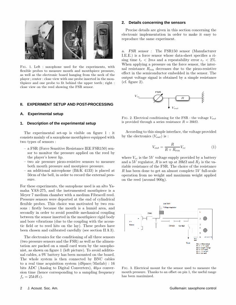
Fig. 1. Left : saxophone used for the experiments, withflexible probes to measure mouth and mouthpiece pressure,as well as the electronic board hanging from the neck of theplayer ; center : close view with one probe inserted in the mou-thpiece and one probe to fit behind the upper teeth ; right :close view on the reed showing the FSR sensor.

II. EXPERIMENT SETUP AND POST-PROCESSING

A. Experimental setup

1. Description of the experimental setup

The experimental set-up is visible on figure 1 : itconsists mainly of a saxophone mouthpiece equipped withtwo types of sensors :

– a FSR (Force Sensitive Resistance IEE FSR150) sen-sor to monitor the pressure applied on the reed bythe player’s lower lip.

– two air pressure piezo-resistive sensors to measureboth mouth pressure and moutpiece pressure.

– an additional microphone (B&K 4133) is placed at50cm of the bell, in order to record the external pres-sure.

For these experiments, the saxophone used is an alto Ya-maha YAS-275, and the instrumented mouthpiece is aMeyer 7 medium chamber with a medium Fibracell reed.Pressure sensors were deported at the end of cylindricalflexible probes. This choice was motivated by two rea-sons : firstly because the mouth is a humid area, andsecondly in order to avoid possible mechanical couplingbetween the sensor inserted in the mouthpiece rigid bodyand bore vibrations (due to the coupling with the acous-tic field or to reed hits on the lay). These probes havebeen chosen and calibrated carefully (see section II A 3).

The electronics for the conditioning of all three sensors(two pressure sensors and the FSR) as well as the alimen-tation are packed on a small card worn by the saxopho-nist, as shown on figure 1 (left picture). To avoid additio-nal cables, a 9V battery has been mounted on the board.The whole system is then connected by BNC cablesto a real time acquisition system (dSpace/Matlab) : 16bits ADC (Analog to Digital Converters), 40µs conver-sion time (hence corresponding to a sampling frequencyfs = 25kHz).

2. Details concerning the sensors

Precise details are given in this section concerning theelectronic implementation in order to make it easy toreproduce the same experiment.

a. FSR sensor : The FSR150 sensor (ManufacturerI.E.E.) is a force sensor whose data-sheet specifies a ri-sing time tr < 2ms and a repeatability error ǫr < 2%.When applying a pressure on the force sensor, the inter-nal resistance Rfsr decreases due to the piezo-resistiveeffect in the semiconductor embedded in the sensor. Theoutput voltage signal is obtained by a simple resistance(cf. figure 2).

Vout

R

FSR

Vcc

Fig. 2. Electrical conditioning for the FSR : the voltage Vout

is provided through a series resistance R = 39kΩ.

According to this simple interface, the voltage providedby the electronics (Vout) is :

Vout =R

R + Rfsr

Vcc (1)

where Vcc is the 5V voltage supply provided by a batteryand a 5V regulator, R is set up at 39kΩ and Rf is the va-riable resistance of the FSR. The choice of the resistanceR has been done to get an almost complete 5V full-scaleoperation from no weight and maximum weight appliedon the reed (around 900g).

Fig. 3. Electrical mount for the sensor used to measure themouth pressure. Thanks to an offset on pin 1, the useful rangehas been maximized.

2 J. Acoust. Soc. Am. Guillemain: saxophone control

b. Pressure sensors : The two pressure sensors usedfor the experiments are piezo-resistive ASCX05 DN, i.e.with a range of 5Psi differential pressure (5Psi ≃ 35kPa).These devices are characterized for operation from asingle 5V dc-supply. For this purpose, a 9V -battery witha voltage regulator (LM -7805) provide a very stable vol-tage supply (which is light enough to be mounted on theportable board). The time response specified in data-sheet is about 100µs. The pressure sensors as well arefixed on the electronics board.

The pressure sensor dedicated to the mouth pressuremeasurement provides a voltage which is always positive,due to an offset voltage applied on its first pin (see figure3). This has been done in order to have a maximum usefulrange. For the mouthpiece pressure, since we measure asignal centered around 0 (acoustic pressure), no offsetis applied since the pressure sensor yields a voltage of2.3V without differential pressure applied on it in orderto operate for differential pressure over the 4.5V full scalerange.

3. Calibration

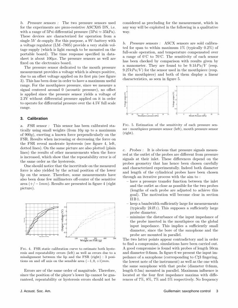
a. FSR sensor : This sensor has been calibrated sta-tically using small weights (from 10g up to a maximumof 900g), exerting a known force perpendicularly on theFSR. Results when increasing or decreasing the force onthe FSR reveal moderate hysteresis (see figure 4, left,dotted lines). On the same picture are also plotted (plainlines) the results of other measurements when the forceis increased, which show that the repeatability error is ofthe same order as the hysteresis.

One should notice that the incertitude on the measuredforce is also yielded by the actual position of the lowerlip on the sensor. Therefore, some measurements havealso been done few millimeters off-center of the sensitivearea (+/−1mm). Results are presented in figure 4 (rightpicture).

! "!! #!! $!! %!! &!! '!! (!! )!! *!!!

!+&

"

"+&

#

#+&

$

$+&

%

%+&

,-./0123-4/54/

62718/3055.7293-:3/823;<=3>1?

100 200 300 400 5000

0.5

1

1.5

2

2.5

3

3.5

Weight on FSR (g)

Out

put v

olta

ge (

V)

Fig. 4. FSR static calibration curve to estimate both hyste-resis and repeatability errors (left) as well as errors due to amisalignment between the lip and the FSR (right) : 3 posi-tions on and off axis on the sensible area (−1, 0, +1)mm.

Errors are of the same order of magnitude. Therefore,since the position of the player’s lower lip cannot be gua-ranteed, repeatability or hysteresis errors should not be

considered as precluding for the measurement, which inany way will be exploited in the following in a qualitativeway.

b. Pressure sensors : ASCX sensors are sold calibra-ted for span to within maximum 1% (typically 0.2%) offull-scale operation, and temperature compensated overa range of 0 C to 70 C. The sensitivity of each sensorhas been checked by comparison with results given bya manometer. They are found to be 9.1kPa/V (resp.9.27kPa/V ) for the sensor used in the mouthpiece (resp.in the mouthpiece) and both of them display a linearcharacteristics, as seen in figure 5.

−25 −20 −15 −10 −5 0 5 10 150

1

2

3

4

5

Mouthpiece pressure (kPa)

Vol

tage

out

put (

V)

−5 0 5 10 15 20 250

0.5

1

1.5

2

2.5

3

Mouth Pressure (kPa)

Vol

tage

out

put (

V)

Fig. 5. Estimation of the sensitivity of each pressure sen-sor : mouthpiece pressure sensor (left), mouth pressure sensor(right).

c. Probes : It is obvious that pressure signals measu-red at the outlet of the probes are different from pressuresignals at their inlet. These differences depend on theprobes geometry that has hence been chosen carefullyand characterized experimentally. Indeed both diameterand length of the cylindrical probes have been chosenthrough an iterative process with the aim to :

– have a pressure transfer function between the inletand the outlet as close as possible for the two probes(lengths of each probe are adjusted to achieve thisgoal). The motivation will become clear in sectionII B 1.

– keep a bandwidth sufficiently large for measurements(typically 2kHz). This supposes a sufficiently largeprobe diameter.

– minimize the disturbance of the input impedance ofthe probe inserted in the mouthpiece on the globalinput impedance. This implies a sufficiently smalldiameter, since the bore of the saxophone and theprobe are mounted in parallel.

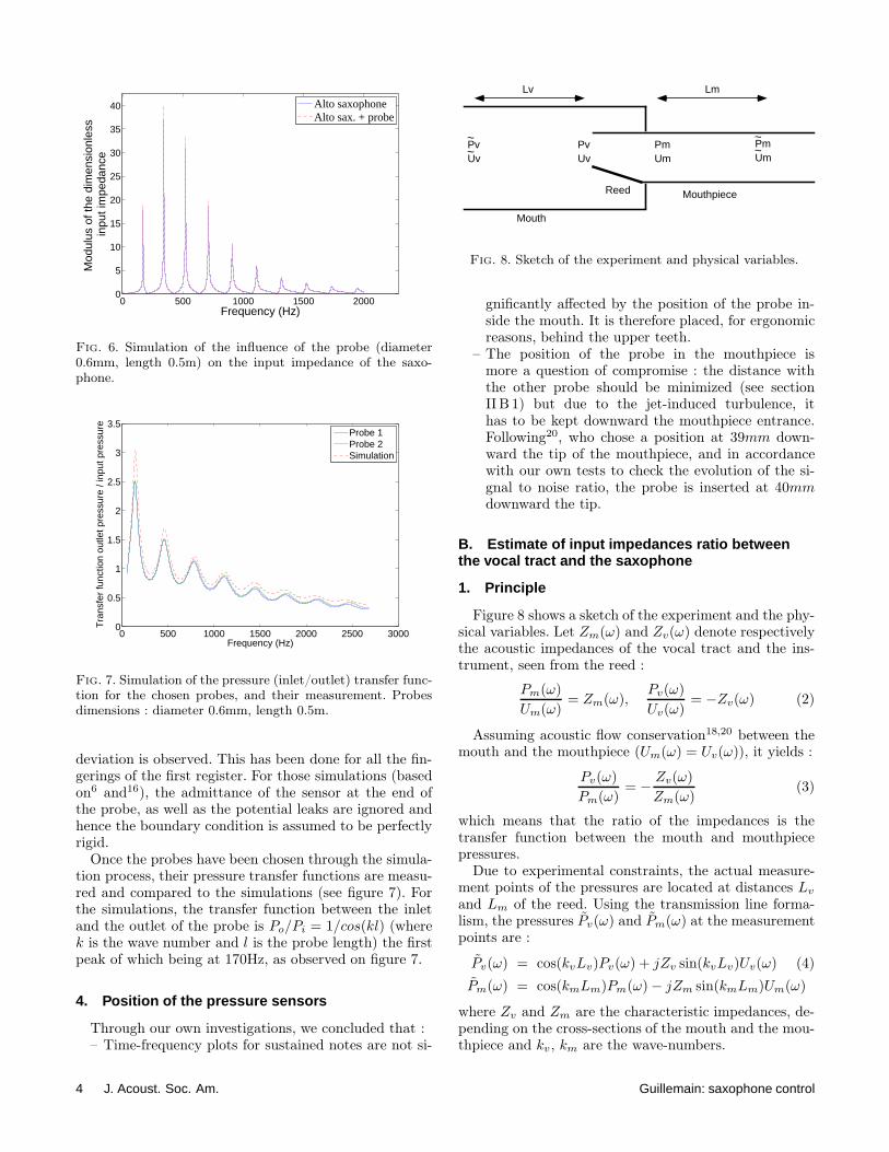
The two latter points appear contradictory and in orderto find a compromise, simulations have been carried out.A good compromise is found with probes of length 50cmand diameter 0.6mm. In figure 6 we present the input im-pedance of a saxophone (corresponding to C♯3 fingering,the lowest note of the instrument) as well as the one withthe same saxophone with that probe (diameter 0.6mm,length 0.5m) mounted in parallel. Maximum influence islocated at the four first impedance maxima with diffe-rences of 7%, 8%, 7% and 5% respectively. No frequency


0 500 1000 1500 20000

5

10

15

20

25

30

35

40

Frequency (Hz)

Mod

ulus

of t

he d

imen

sion

less

in

put i

mpe

danc

e

Alto saxophoneAlto sax. + probe

Fig. 6. Simulation of the influence of the probe (diameter0.6mm, length 0.5m) on the input impedance of the saxo-phone.

0 500 1000 1500 2000 2500 30000

0.5

1

1.5

2

2.5

3

3.5

Frequency (Hz)

Tra

nsfe

r fu

nctio

n ou

tlet p

ress

ure

/ inp

ut p

ress

ure

Probe 1Probe 2Simulation

Fig. 7. Simulation of the pressure (inlet/outlet) transfer func-tion for the chosen probes, and their measurement. Probesdimensions : diameter 0.6mm, length 0.5m.

deviation is observed. This has been done for all the fin-gerings of the first register. For those simulations (basedon6 and16), the admittance of the sensor at the end ofthe probe, as well as the potential leaks are ignored andhence the boundary condition is assumed to be perfectlyrigid.

Once the probes have been chosen through the simula-tion process, their pressure transfer functions are measu-red and compared to the simulations (see figure 7). Forthe simulations, the transfer function between the inletand the outlet of the probe is Po/Pi = 1/cos(kl) (wherek is the wave number and l is the probe length) the firstpeak of which being at 170Hz, as observed on figure 7.

4. Position of the pressure sensors

Through our own investigations, we concluded that :– Time-frequency plots for sustained notes are not si-

Reed Mouthpiece

PmUm

PvUv

PvUv

Mouth

PmUm

~~

~~

Lv Lm

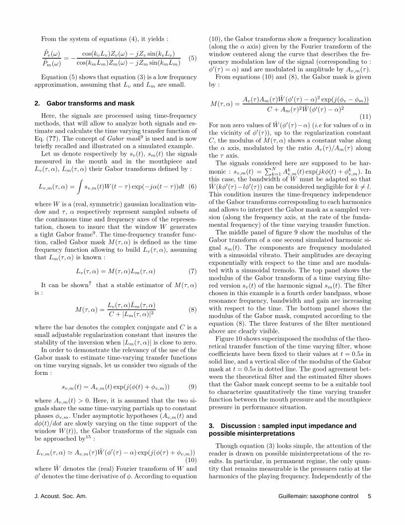
Fig. 8. Sketch of the experiment and physical variables.

gnificantly affected by the position of the probe in-side the mouth. It is therefore placed, for ergonomicreasons, behind the upper teeth.

– The position of the probe in the mouthpiece ismore a question of compromise : the distance withthe other probe should be minimized (see sectionII B 1) but due to the jet-induced turbulence, ithas to be kept downward the mouthpiece entrance.Following20, who chose a position at 39mm down-ward the tip of the mouthpiece, and in accordancewith our own tests to check the evolution of the si-gnal to noise ratio, the probe is inserted at 40mmdownward the tip.

B. Estimate of input impedances ratio betweenthe vocal tract and the saxophone

1. Principle

Figure 8 shows a sketch of the experiment and the phy-sical variables. Let Zm(ω) and Zv(ω) denote respectivelythe acoustic impedances of the vocal tract and the ins-trument, seen from the reed :

Pm(ω)

Um(ω)= Zm(ω),

Pv(ω)

Uv(ω)= −Zv(ω) (2)

Assuming acoustic flow conservation18,20 between themouth and the mouthpiece (Um(ω) = Uv(ω)), it yields :

Pv(ω)

Pm(ω)= −

Zv(ω)

Zm(ω)(3)

which means that the ratio of the impedances is thetransfer function between the mouth and mouthpiecepressures.

Due to experimental constraints, the actual measure-ment points of the pressures are located at distances Lv

and Lm of the reed. Using the transmission line forma-lism, the pressures Pv(ω) and Pm(ω) at the measurementpoints are :

Pv(ω) = cos(kvLv)Pv(ω) + jZv sin(kvLv)Uv(ω) (4)

Pm(ω) = cos(kmLm)Pm(ω) − jZm sin(kmLm)Um(ω)

where Zv and Zm are the characteristic impedances, de-pending on the cross-sections of the mouth and the mou-thpiece and kv, km are the wave-numbers.


From the system of equations (4), it yields :

Pv(ω)

Pm(ω)= −

cos(kvLv)Zv(ω) − jZv sin(kvLv)

cos(kmLm)Zm(ω) − jZm sin(kmLm)(5)

Equation (5) shows that equation (3) is a low frequencyapproximation, assuming that Lv and Lm are small.

2. Gabor transforms and mask

Here, the signals are processed using time-frequencymethods, that will allow to analyze both signals and es-timate and calculate the time varying transfer function ofEq. (??). The concept of Gabor mask

9 is used and is nowbriefly recalled and illustrated on a simulated example.

Let us denote respectively by sv(t), sm(t) the signalsmeasured in the mouth and in the mouthpiece andLv(τ, α), Lm(τ, α) their Gabor transforms defined by :

Lv,m(τ, α) =

∫sv,m(t)W (t − τ) exp(−jα(t − τ))dt (6)

where W is a (real, symmetric) gaussian localization win-dow and τ , α respectively represent sampled subsets ofthe continuous time and frequency axes of the represen-tation, chosen to insure that the window W generatesa tight Gabor frame9. The time-frequency transfer func-tion, called Gabor mask M(τ, α) is defined as the timefrequency function allowing to build Lv(τ, α), assumingthat Lm(τ, α) is known :

Lv(τ, α) = M(τ, α)Lm(τ, α) (7)

It can be shown? that a stable estimator of M(τ, α)is :

M(τ, α) =Lv(τ, α)Lm(τ, α)

C + |Lm(τ, α)|2(8)

where the bar denotes the complex conjugate and C is asmall adjustable regularization constant that insures thestability of the inversion when |Lm(τ, α)| is close to zero.

In order to demonstrate the relevancy of the use of theGabor mask to estimate time-varying transfer functionson time varying signals, let us consider two signals of theform :

sv,m(t) = Av,m(t) exp(j(φ(t) + φv,m)) (9)

where Av,m(t) > 0. Here, it is assumed that the two si-gnals share the same time-varying partials up to constantphases φv,m. Under asymptotic hypotheses (Av,m(t) anddφ(t)/dot are slowly varying on the time support of thewindow W (t)), the Gabor transforms of the signals canbe approached by15 :

Lv,m(τ, α) ≃ Av,m(τ)W (φ′(τ) − α) exp(j(φ(τ) + φv,m))(10)

where W denotes the (real) Fourier transform of W andφ′ denotes the time derivative of φ. According to equation

(10), the Gabor transforms show a frequency localization(along the α axis) given by the Fourier transform of thewindow centered along the curve that describes the fre-quency modulation law of the signal (corresponding to :φ′(τ) = α) and are modulated in amplitude by Av,m(τ).

From equations (10) and (8), the Gabor mask is givenby :

M(τ, α) =Av(τ)Am(τ)W (φ′(τ) − α)2 exp(j(φv − φm))

C + Am(τ)2W (φ′(τ) − α)2

(11)

For non zero values of W (φ′(τ)−α) (i.e for values of α inthe vicinity of φ′(τ)), up to the regularization constantC, the modulus of M(τ, α) shows a constant value alongthe α axis, modulated by the ratio Av(τ)/Am(τ) alongthe τ axis.

The signals considered here are supposed to be har-

monic : sv,m(t) =∑N

k=1 Akv,m(t) exp(jkφ(t) + φk

v,m). Inthis case, the bandwidth of W must be adapted so thatW (kφ′(τ)− lφ′(τ)) can be considered negligible for k 6= l.This condition insures the time-frequency independenceof the Gabor transforms corresponding to each harmonicsand allows to interpret the Gabor mask as a sampled ver-sion (along the frequency axis, at the rate of the funda-mental frequency) of the time varying transfer function.

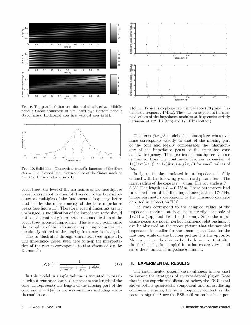
The middle panel of figure 9 show the modulus of theGabor transform of a one second simulated harmonic si-gnal sm(t). The components are frequency modulatedwith a sinusoidal vibrato. Their amplitudes are decayingexponentially with respect to the time and are modula-ted with a sinusoidal tremolo. The top panel shows themodulus of the Gabor transform of a time varying filte-red version sv(t) of the harmonic signal sm(t). The filterchosen in this example is a fourth order bandpass, whoseresonance frequency, bandwidth and gain are increasingwith respect to the time. The bottom panel shows themodulus of the Gabor mask, computed according to theequation (8). The three features of the filter mentionedabove are clearly visible.

Figure 10 shows superimposed the modulus of the theo-retical transfer function of the time varying filter, whosecoefficients have been fixed to their values at t = 0.5s insolid line, and a vertical slice of the modulus of the Gabormask at t = 0.5s in dotted line. The good agreement bet-ween the theoretical filter and the estimated filter showsthat the Gabor mask concept seems to be a suitable toolto characterize quantitatively the time varying transferfunction between the mouth pressure and the mouthpiecepressure in performance situation.

3. Discussion : sampled input impedance andpossible misinterpretations

Though equation (3) looks simple, the attention of thereader is drawn on possible misinterpretations of the re-sults. In particular, in permanent regime, the only quan-tity that remains measurable is the pressures ratio at theharmonics of the playing frequency. Independently of the


Time (s)

Sv

(kH

z)

0 0.1 0.2 0.3 0.4 0.5 0.6 0.7 0.8 0.9

-1.5

-1

-0.5

0

0.5

1

1.5

2

Time (s)

Sm

(kH

z)

0 0.1 0.2 0.3 0.4 0.5 0.6 0.7 0.8 0.9

-1.5

-1

-0.5

0

0.2

0.4

0.6

0.8

1

Time (s)

Gab

or m

ask

mod

ulus

(kH

z)

0 0.1 0.2 0.3 0.4 0.5 0.6 0.7 0.8 0.9

-1.5

-1

-0.5

0 0

2

4

6

8

Fig. 9. Top panel : Gabor transform of simulated sv ; Middlepanel : Gabor transform of simulated sm ; Bottom panel :Gabor mask. Horizontal axes in s, vertical axes in kHz.

0 0.2 0.4 0.6 0.8 1 1.2 1.4 1.6 1.8 20

1

2

3

4

Tra

nsfe

r fu

nctio

n

Frequency (kHz)

Fig. 10. Solid line : Theoretical transfer function of the filterat t = 0.5s. Dotted line : Vertical slice of the Gabor mask att = 0.5s. Horizontal axis in kHz.

vocal tract, the level of the harmonics of the mouthpiecepressure is related to a sampled version of the bore impe-dance at multiples of the fundamental frequency, hencemodified by the inharmonicity of the bore impedancepeaks (see figure 11). Therefore, even if fingerings are letunchanged, a modification of the impedance ratio shouldnot be systematically interpreted as a modification of thevocal tract acoustic impedance. This is a key point sincethe sampling of the instrument input impedance is tre-mendously altered as the playing frequency is changed.

This is illustrated through simulation (see figure 11).The impedance model used here to help the interpreta-tion of the results corresponds to that discussed e.g. byDalmont6 :

Ze(ω) =1

1j tan(kL) + 1

jkxe

+ jkxe

3

(12)

In this model, a simple volume is mounted in paral-lel with a truncated cone. L represents the length of thecone, xe represents the length of the missing part of thecone and k = k(ω) is the wave-number including visco-thermal losses.

0 200 400 600 800 1000 1200 14000

5

10

15

20

25

30

frequency(Hz)

dim

ensi

onle

ss im

peda

nce

mod

ulus

0 200 400 600 800 1000 1200 14000

5

10

15

20

25

30

frequency(Hz)

dim

ensi

onle

ss im

peda

nce

mod

ulus

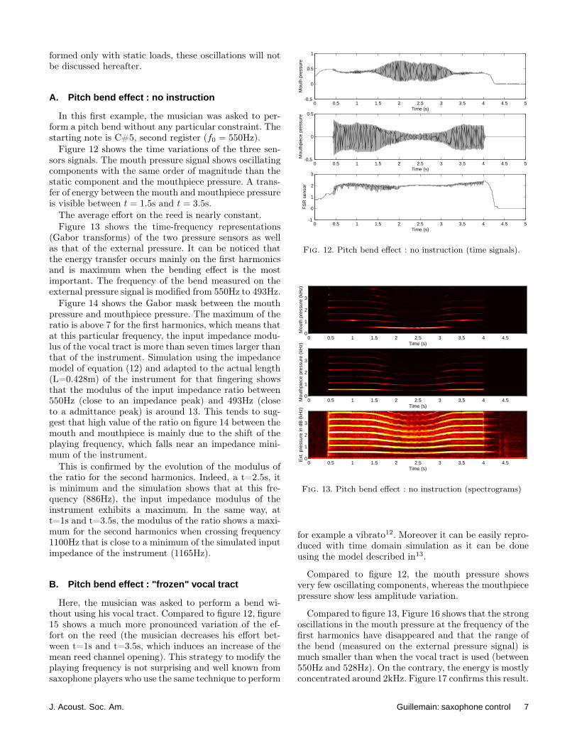
Fig. 11. Typical saxophone input impedance (F3 piano, fun-damental frequency 174Hz). The stars correspond to the sam-pled values of the impedance modulus at frequencies strictlyharmonic of 172.1Hz (top) and 176.1Hz (bottom).

The term jkxe/3 models the mouthpiece whose vo-lume corresponds exactly to that of the missing partof the cone and ideally compensates the inharmoni-city of the impedance peaks of the truncated coneat low frequency. This particular mouthpiece volumeis derived from the continuous fraction expansion of1/(j tan(kxe)) ≃ 1/(jkxe) + jkxe/3 for small values ofkxe.

In figure 11, the simulated input impedance is fullydefined with the following geometrical parameters : Theinput radius of the cone is r = 6mm. The top angle is θ =3.36 . The length is L = 0.755m. These parameters leadto a maximum of the first impedance peak at 174.1Hz.These parameters correspond to the glissando exampledepicted in subsection III C.

The stars correspond to the sampled values of theimpedance modulus at frequencies strictly harmonic of172.1Hz (top) and 176.1Hz (bottom). Since the impe-dance peaks are not in perfect harmonic relationships, itcan be observed on the upper picture that the sampledimpedance is smaller for the second peak than for thefirst one, while on the bottom picture it is the opposite.Moreover, it can be observed on both pictures that afterthe third peak, the sampled impedances are very smallsince the stars fall in impedance minima.

III. EXPERIMENTAL RESULTS

The instrumented saxophone mouthpiece is now usedto inspect the strategies of an experienced player. Notethat in the experiments discussed below, the FSR signalshows both a quasi-static component and an oscillatingcomponent sharing the same frequency content as thepressure signals. Since the FSR calibration has been per-


formed only with static loads, these oscillations will notbe discussed hereafter.

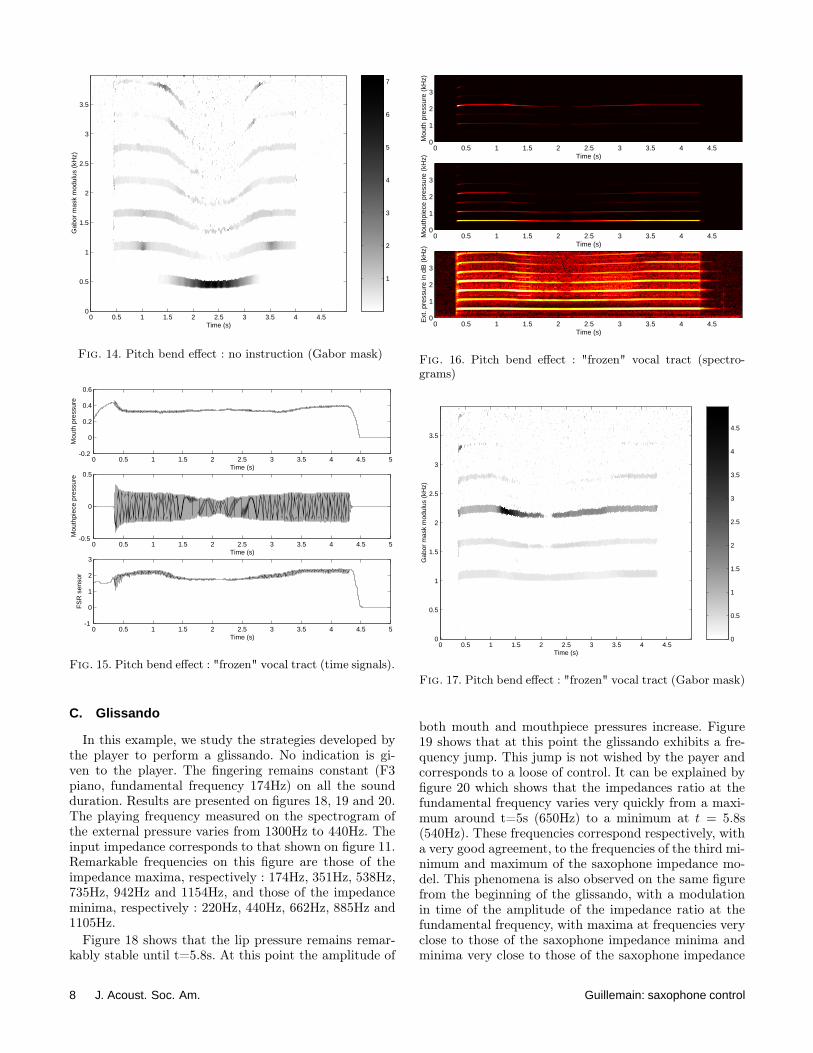
A. Pitch bend effect : no instruction

In this first example, the musician was asked to per-form a pitch bend without any particular constraint. Thestarting note is C#5, second register (f0 = 550Hz).

Figure 12 shows the time variations of the three sen-sors signals. The mouth pressure signal shows oscillatingcomponents with the same order of magnitude than thestatic component and the mouthpiece pressure. A trans-fer of energy between the mouth and mouthpiece pressureis visible between t = 1.5s and t = 3.5s.

The average effort on the reed is nearly constant.Figure 13 shows the time-frequency representations

(Gabor transforms) of the two pressure sensors as wellas that of the external pressure. It can be noticed thatthe energy transfer occurs mainly on the first harmonicsand is maximum when the bending effect is the mostimportant. The frequency of the bend measured on theexternal pressure signal is modified from 550Hz to 493Hz.

Figure 14 shows the Gabor mask between the mouthpressure and mouthpiece pressure. The maximum of theratio is above 7 for the first harmonics, which means thatat this particular frequency, the input impedance modu-lus of the vocal tract is more than seven times larger thanthat of the instrument. Simulation using the impedancemodel of equation (12) and adapted to the actual length(L=0.428m) of the instrument for that fingering showsthat the modulus of the input impedance ratio between550Hz (close to an impedance peak) and 493Hz (closeto a admittance peak) is around 13. This tends to sug-gest that high value of the ratio on figure 14 between themouth and mouthpiece is mainly due to the shift of theplaying frequency, which falls near an impedance mini-mum of the instrument.

This is confirmed by the evolution of the modulus ofthe ratio for the second harmonics. Indeed, a t=2.5s, itis minimum and the simulation shows that at this fre-quency (886Hz), the input impedance modulus of theinstrument exhibits a maximum. In the same way, att=1s and t=3.5s, the modulus of the ratio shows a maxi-mum for the second harmonics when crossing frequency1100Hz that is close to a minimum of the simulated inputimpedance of the instrument (1165Hz).

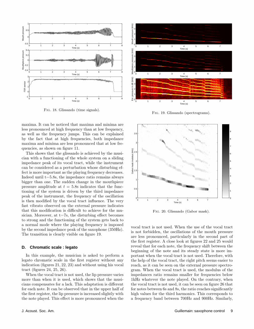
B. Pitch bend effect : "frozen" vocal tract

Here, the musician was asked to perform a bend wi-thout using his vocal tract. Compared to figure 12, figure15 shows a much more pronounced variation of the ef-fort on the reed (the musician decreases his effort bet-ween t=1s and t=3.5s, which induces an increase of themean reed channel opening). This strategy to modify theplaying frequency is not surprising and well known fromsaxophone players who use the same technique to perform

0 0.5 1 1.5 2 2.5 3 3.5 4 4.5 5-0.5

0

0.5

1

Mou

th p

ress

ure

Time (s)

0 0.5 1 1.5 2 2.5 3 3.5 4 4.5 5-0.5

0

0.5

Mou

thpi

ece

pres

sure

Time (s)

0 0.5 1 1.5 2 2.5 3 3.5 4 4.5 5-1

0

1

2

3

FS

R s

enso

r

Time (s)

Fig. 12. Pitch bend effect : no instruction (time signals).

Mou

th p

ress

ure

(kH

z)

Time (s)0 0.5 1 1.5 2 2.5 3 3.5 4 4.5

0

1

2

3M

outh

piec

e pr

essu

re (

kHz)

Time (s)0 0.5 1 1.5 2 2.5 3 3.5 4 4.5

0

1

2

3

Ext

. pre

ssur

e in

dB

(kH

z)

Time (s)0 0.5 1 1.5 2 2.5 3 3.5 4 4.5

0

1

2

3

Fig. 13. Pitch bend effect : no instruction (spectrograms)

for example a vibrato12. Moreover it can be easily repro-duced with time domain simulation as it can be doneusing the model described in13.

Compared to figure 12, the mouth pressure showsvery few oscillating components, whereas the mouthpiecepressure show less amplitude variation.

Compared to figure 13, Figure 16 shows that the strongoscillations in the mouth pressure at the frequency of thefirst harmonics have disappeared and that the range ofthe bend (measured on the external pressure signal) ismuch smaller than when the vocal tract is used (between550Hz and 528Hz). On the contrary, the energy is mostlyconcentrated around 2kHz. Figure 17 confirms this result.


Time (s)

Gab

or m

ask

mod

ulus

(kH

z)

0 0.5 1 1.5 2 2.5 3 3.5 4 4.50

0.5

1

1.5

2

2.5

3

3.5

1

2

3

4

5

6

7

Fig. 14. Pitch bend effect : no instruction (Gabor mask)

0 0.5 1 1.5 2 2.5 3 3.5 4 4.5 5-0.2

0

0.2

0.4

0.6

Mou

th p

ress

ure

Time (s)

0 0.5 1 1.5 2 2.5 3 3.5 4 4.5 5-0.5

0

0.5

Mou

thpi

ece

pres

sure

Time (s)

0 0.5 1 1.5 2 2.5 3 3.5 4 4.5 5-1

0

1

2

3

FS

R s

enso

r

Time (s)

Fig. 15. Pitch bend effect : "frozen" vocal tract (time signals).

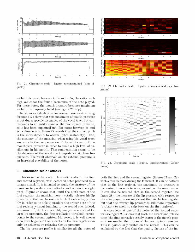
C. Glissando

In this example, we study the strategies developed bythe player to perform a glissando. No indication is gi-ven to the player. The fingering remains constant (F3piano, fundamental frequency 174Hz) on all the soundduration. Results are presented on figures 18, 19 and 20.The playing frequency measured on the spectrogram ofthe external pressure varies from 1300Hz to 440Hz. Theinput impedance corresponds to that shown on figure 11.Remarkable frequencies on this figure are those of theimpedance maxima, respectively : 174Hz, 351Hz, 538Hz,735Hz, 942Hz and 1154Hz, and those of the impedanceminima, respectively : 220Hz, 440Hz, 662Hz, 885Hz and1105Hz.

Figure 18 shows that the lip pressure remains remar-kably stable until t=5.8s. At this point the amplitude of

Mou

th p

ress

ure

(kH

z)

Time (s)0 0.5 1 1.5 2 2.5 3 3.5 4 4.5

0

1

2

3

Mou

thpi

ece

pres

sure

(kH

z)

Time (s)0 0.5 1 1.5 2 2.5 3 3.5 4 4.5

0

1

2

3

Ext

. pre

ssur

e in

dB

(kH

z)

Time (s)0 0.5 1 1.5 2 2.5 3 3.5 4 4.5

0

1

2

3

Fig. 16. Pitch bend effect : "frozen" vocal tract (spectro-grams)

Time (s)

Gab

or m

ask

mod

ulus

(kH

z)

0 0.5 1 1.5 2 2.5 3 3.5 4 4.50

0.5

1

1.5

2

2.5

3

3.5

0

0.5

1

1.5

2

2.5

3

3.5

4

4.5

Fig. 17. Pitch bend effect : "frozen" vocal tract (Gabor mask)

both mouth and mouthpiece pressures increase. Figure19 shows that at this point the glissando exhibits a fre-quency jump. This jump is not wished by the payer andcorresponds to a loose of control. It can be explained byfigure 20 which shows that the impedances ratio at thefundamental frequency varies very quickly from a maxi-mum around t=5s (650Hz) to a minimum at t = 5.8s(540Hz). These frequencies correspond respectively, witha very good agreement, to the frequencies of the third mi-nimum and maximum of the saxophone impedance mo-del. This phenomena is also observed on the same figurefrom the beginning of the glissando, with a modulationin time of the amplitude of the impedance ratio at thefundamental frequency, with maxima at frequencies veryclose to those of the saxophone impedance minima andminima very close to those of the saxophone impedance


0 1 2 3 4 5 6 7 8-0.5

0

0.5

1M

outh

pre

ssur

e

Time (s)

0 1 2 3 4 5 6 7 8-0.4

-0.2

0

0.2

0.4

Mou

thpi

ece

pres

sure

Time (s)

0 1 2 3 4 5 6 7 8-1

0

1

2

3

FS

R s

enso

r

Time (s)

Fig. 18. Glissando (time signals).

maxima. It can be noticed that maxima and minima areless pronounced at high frequency than at low frequency,as well as the frequency jumps. This can be explainedby the fact that at high frequencies, both impedancemaxima and minima are less pronounced that at low fre-quencies, as shown on figure 11.

This shows that the glissando is achieved by the musi-cian with a functioning of the whole system on a slidingimpedance peak of its vocal tract, while the instrumentcan be considered as a perturbation whose disturbing ef-fect is more important as the playing frequency decreases.Indeed until t=5.8s, the impedance ratio remains alwaysbigger than one. The sudden change in the mouthpiecepressure amplitude at t = 5.8s indicates that the func-tioning of the system is driven by the third impedancepeak of the instrument, the frequency of the oscillationis then modified by the vocal tract influence. The veryfast vibrato observed on the external pressure indicatesthat this modification is difficult to achieve for the mu-sician. Moreover, at t=7s, the disturbing effect becomesto strong and the functioning of the system gets back toa normal mode where the playing frequency is imposedby the second impedance peak of the saxophone (350Hz).The transition is clearly visible on figure 19.

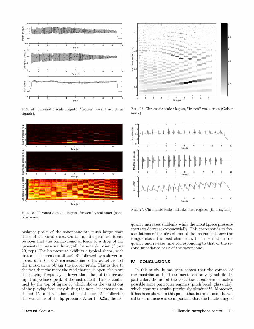
D. Chromatic scale : legato

In this example, the musician is asked to perform alegato chromatic scale in the first register without anyindication (figures 21, 22, 23) and without using his vocaltract (figures 24, 25, 26).

When the vocal tract is not used, the lip pressure variesmore than when it is used, which shows that the musi-cians compensates for a lack. This adaptation is differentfor each note. It can be observed that in the upper half ofthe first register, the lip pressure is increased slightly withthe note played. This effect is more pronounced when the

Mou

th p

ress

ure

(kH

z)

Time (s)0 1 2 3 4 5 6 7

0

1

2

3

Mou

thpi

ece

pres

sure

(kH

z)

Time (s)0 1 2 3 4 5 6 7

0

1

2

3

Ext

. pre

ssur

e in

dB

(kH

z)

Time (s)0 1 2 3 4 5 6 7

0

1

2

3

Fig. 19. Glissando (spectrograms).

Time (s)

Gab

or m

ask

mod

ulus

(kH

z)

0 1 2 3 4 5 6 70

0.5

1

1.5

2

2.5

3

3.5

0

1

2

3

4

5

6

7

8

9

Fig. 20. Glissando (Gabor mask).

vocal tract is not used. When the use of the vocal tractis not forbidden, the oscillations of the mouth pressureare less pronounced, particularly in the second part ofthe first register. A close look at figures 22 and 25 wouldreveal that for each note, the frequency shift between thebeginning of the note and its steady state is more im-portant when the vocal tract is not used. Therefore, withthe help of the vocal tract, the right pitch seems easier toreach, as it can be seen on the external pressure spectro-gram. When the vocal tract is used, the modulus of theimpedances ratio remains smaller for frequencies below1kHz whatever the note played. On the contrary, whenthe vocal tract is not used, it can be seen on figure 26 thatfor notes between 6s and 8s, the ratio reaches significantlyhigh values for the third harmonics. This corresponds toa frequency band between 700Hz and 900Hz. Similarly,


0 1 2 3 4 5 6 7 8 9 10-0.2

0

0.2

0.4

0.6M

outh

pre

ssur

e

Time (s)

0 1 2 3 4 5 6 7 8 9 10-2

-1

0

1

Mou

thpi

ece

pres

sure

Time (s)

0 1 2 3 4 5 6 7 8 9 10-1

0

1

2

3

FS

R s

enso

r

Time (s)

Fig. 21. Chromatic scale : legato, unconstrained (time si-gnals).

within this band, between t=3s and t=5s, the ratio reachhigh values for the fourth harmonics of the note played.For these notes, the mouth pressure becomes maximumwithin this frequency band (see figure 25, top).

Impedances calculations for several bore lengths usingformula (12) show that this maximum of mouth pressureis not due a specific resonance of the vocal tract but cor-responds to an antiformant of the mouthpiece pressure,as it has been explained in6. For notes between 6s and8s, a close look at figure 25 reveals that the correct pitchis the most difficult to obtain (pitch instability). Here,the strategy of the musician when using his vocal tractseems to be the compensation of the antiformant of themouthpiece pressure in order to avoid a high level of os-cillations in his mouth. This compensation seems to bethe decrease of the vocal tract impedance at these fre-quencies. The result observed on the external pressure isan increased playability of the notes.

E. Chromatic scale : attacks

This example deals with chromatic scales in the firstand second registers, with detached notes produced by atongue attack. It is intended to study the strategy of themusician to produce neat attacks and obtain the rightpitch. Figure 27 shows that, until the ninth note of thefirst register, the musician nearly totally releases his lippressure on the reed before the birth of each note, proba-bly in order to be able to produce the proper note of thefirst register without jumping to the second one. Indeed,as shown in17, the linear stability analysis reveals that forlarge lip pressures, the first oscillation threshold corres-ponds to the second register. Moreover, it is well knowneven from beginners that attacks on the first register canonly be achieved by releasing the lip pressure.

The lip pressure profile is similar for all the notes of

Mou

th p

ress

ure

(kH

z)

Time (s)0 1 2 3 4 5 6 7 8 9

0

1

2

3

Mou

thpi

ece

pres

sure

(kH

z)

Time (s)0 1 2 3 4 5 6 7 8 9

0

1

2

3

Ext

. pre

ssur

e in

dB

(kH

z)

Time (s)0 1 2 3 4 5 6 7 8 9

0

1

2

3

Fig. 22. Chromatic scale : legato, unconstrained (spectro-grams).

Time (s)

Gab

or m

ask

mod

ulus

(kH

z)

0 1 2 3 4 5 6 7 8 90

0.5

1

1.5

2

2.5

3

3.5

0

0.5

1

1.5

2

2.5

3

Fig. 23. Chromatic scale : legato, unconstrained (Gabormask).

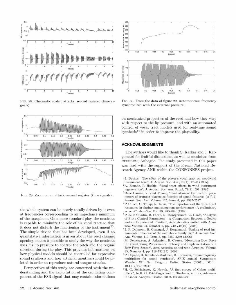
both the first and the second register (figures 27 and 28)with a fast increase during the transient. It can be noticedthat in the first register, the maximum lip pressure isincreasing from note to note, as well as the mean value.It can also be noticed that in the second register (seefigure 28), the increase of the lip pressure with respect tothe note played is less important than in the first registerbut that the average lip pressure is still more important(probably to avoid to skip back on the first register).

A close look at one of the notes of the second regis-ter (see figure 29) shows that both the attack and releasetime (the time to reach a steady-state) of the mouth pres-sure are smaller than those of the mouthpiece pressure.This is particularly visible on the release. This can beexplained by the fact that the quality factors of the im-


0 1 2 3 4 5 6 7 8 9 10-0.2

0

0.2

0.4

0.6M

outh

pre

ssur

e

Time (s)

0 1 2 3 4 5 6 7 8 9 10-2

-1

0

1

Mou

thpi

ece

pres

sure

Time (s)

0 1 2 3 4 5 6 7 8 9 10-1

0

1

2

3

FS

R s

enso

r

Time (s)

Fig. 24. Chromatic scale : legato, "frozen" vocal tract (timesignals).

Mou

th p

ress

ure

(kH

z)

Time (s)0 1 2 3 4 5 6 7 8 9

0

1

2

3

Mou

thpi

ece

pres

sure

(kH

z)

Time (s)0 1 2 3 4 5 6 7 8 9

0

1

2

3

Ext

. pre

ssur

e in

dB

(kH

z)

Time (s)0 1 2 3 4 5 6 7 8 9

0

1

2

3

Fig. 25. Chromatic scale : legato, "frozen" vocal tract (spec-trograms).

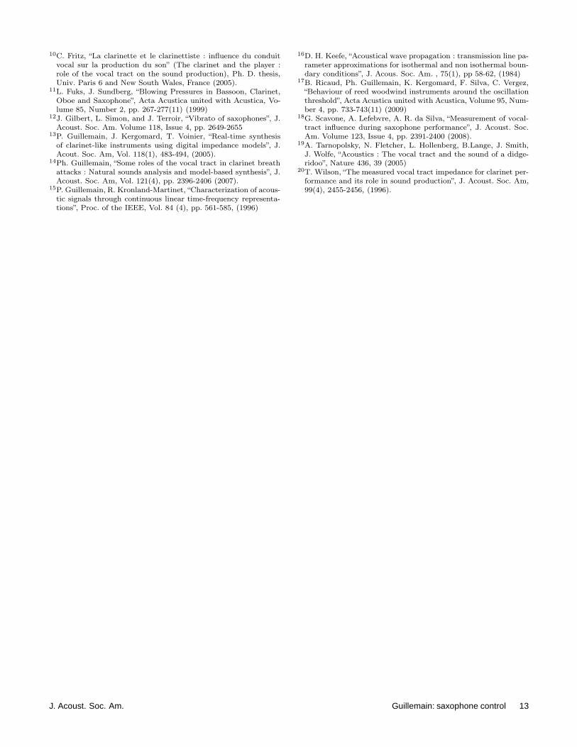
pedance peaks of the saxophone are much larger thanthose of the vocal tract. On the mouth pressure, it canbe seen that the tongue removal leads to a drop of thequasi-static pressure during all the note duration (figure29, top). The lip pressure exhibits a typical shape, withfirst a fast increase until t=0.07s followed by a slower in-crease until t = 0.2s corresponding to the adaptation ofthe musician to obtain the proper pitch. This is due tothe fact that the more the reed channel is open, the morethe playing frequency is lower than that of the secondinput impedance peak of the instrument. This is confir-med by the top of figure 30 which shows the variationsof the playing frequency during the note. It increases un-til t=0.15s and remains stable until t=0.25s, followingthe variations of the lip pressure. After t=0.25s, the fre-

Time (s)

Gab

or m

ask

mod

ulus

(kH

z)

0 1 2 3 4 5 6 7 8 90

0.5

1

1.5

2

2.5

3

3.5

0.5

1

1.5

2

2.5

3

Fig. 26. Chromatic scale : legato, "frozen" vocal tract (Gabormask).

0 1 2 3 4 5 6 7 8 9 10-0.5

0

0.5

1

1.5

Mou

th p

ress

ure

Time (s)

0 1 2 3 4 5 6 7 8 9 10-2

-1

0

1

2

Mou

thpi

ece

pres

sure

Time (s)

0 1 2 3 4 5 6 7 8 9 10-1

0

1

2

3

FS

R s

enso

r

Time (s)

Fig. 27. Chromatic scale : attacks, first register (time signals).

quency increases suddenly while the mouthpiece pressurestarts to decrease exponentially. This corresponds to freeoscillations of the air column of the instrument once thetongue closes the reed channel, with an oscillation fre-quency and release time corresponding to that of the se-cond impedance peak of the saxophone.

IV. CONCLUSIONS

In this study, it has been shown that the control ofthe musician on his instrument can be very subtile. Inparticular, the use of the vocal tract reinforce or makespossible some particular regimes (pitch bend, glissando),which confirms results previously obtained18. Moreover,it has been shown in this paper that in some cases the vo-cal tract influence is so important that the functioning of


0 1 2 3 4 5 6 7 8 9 10-0.5

0

0.5

1

1.5M

outh

pre

ssur

e

Time (s)

0 1 2 3 4 5 6 7 8 9 10-1

0

1

2

Mou

thpi

ece

pres

sure

Time (s)

0 1 2 3 4 5 6 7 8 9 10-1

0

1

2

3

FS

R s

enso

r

Time (s)

Fig. 28. Chromatic scale : attacks, second register (time si-gnals).

0 0.05 0.1 0.15 0.2 0.25 0.3 0.35 0.4 0.45 0.50.5

1

1.5

Mou

th p

ress

ure

Time (s)

0 0.05 0.1 0.15 0.2 0.25 0.3 0.35 0.4 0.45 0.5-1

-0.5

0

0.5

1

Mou

thpi

ece

pres

sure

Time (s)

0 0.05 0.1 0.15 0.2 0.25 0.3 0.35 0.4 0.45 0.50.5

1

1.5

2

2.5

FS

R s

enso

r

Time (s)

Fig. 29. Zoom on an attack, second register (time signals).

the whole system can be nearly totally driven by it evenat frequencies corresponding to an impedance minimumof the saxophone. On a more standard play, the musicianis capable to minimize the role of his vocal tract so thatit does not disturb the functioning of the instrument20.The simple device that has been developed, even if noquantitative information is given about the reed channelopening, makes it possible to study the way the musicianuses his lip pressure to control the pitch and the regimeselection during the play. This provides informations onhow physical models should be controlled for expressivesound synthesis and how artificial mouthes should be pi-loted in order to reproduce natural tongue attacks.

Perspectives of this study are concerned with the un-derstanding and the exploitation of the oscillating com-ponent of the FSR signal that may contain informations

0 0.05 0.1 0.15 0.2 0.25 0.3 0.35 0.4 0.45 0.5350

355

360

365

370

375

380

385

time (s)

Fun

dam

enta

l fre

quen

cy (

Hz)

0 0.05 0.1 0.15 0.2 0.25 0.3 0.35 0.4 0.45 0.5-1

-0.5

0

0.5

1

time (s)

Mou

thpi

ece

pres

sure

Fig. 30. From the data of figure 29, instantaneous frequencysynchronized with the external pressure.

on mechanical properties of the reed and how they varywith respect to the lip pressure, and with an automatedcontrol of vocal tract models used for real-time soundsynthesis14 in order to improve the playability.

ACKNOWLEDGMENTS

The authors would like to thank S. Karkar and J. Ker-gomard for fruitful discussions, as well as musicians fromcefedem, Aubagne. The study presented in this paperwas lead with the support of the French National Re-search Agency ANR within the CONSONNES project.

1J. Backus, “The effect of the player’s vocal tract on woodwindinstrument tone”, J. Acoust. Soc. Am., 78(1), 17-20 (1985).

2A. Benade, P. Hoekje, “Vocal tract effects in wind instrumentregeneration”, J. Acoust. Soc. Am. Suppl, 71(1), 591 (1985).

3Rene Causse, Vincent Freour, “Evaluation of two control para-meters of trumpet players as function of sound features. (A)”, J.Acoust. Soc. Am. Volume 125, Issue 4, pp. 2597-2597

4P. Clinch, G. Troup, L. Harris, “The importance of the vocal tractresonance in clarinet and saxophone performance : A preliminaryaccount”, Acustica, Vol. 50, 280-284, (1982).

5P. de la Cuadra, B. Fabre, N. Montgermont, C. Chafe, “Analysisof Flute Control Parameters : A Comparison Between a Noviceand an Experienced Flautist”, Acta Acustica united with Acus-tica, Volume 94, Number 5, pp. 740-749(10) (2008)

6J. P. Dalmont, B. Gazengel, J. Kergomard, “Scaling of reed ins-truments : The case of the saxophone family (A)”, J. Acoust. Soc.Am. Volume 119, Issue 5, pp. 3259-3259 (2006)

7M. Demoucron, A. Askenfelt, R. Causse, “Measuring Bow Forcein Bowed String Performance : Theory and Implementation of aBow Force Sensor”, Acta Acustica united with Acustica, Volume95, Number 4, pp. 718-732(15) (2009)

8P. Depalle, R. Kronland-Martinet, B. Torresani, “Time-frequencymultipliers for sound synthesis”, SPIE annual SymposiumWavelet XII, San Diego : United States (2007), DOI :10.1117/12.732447

9H. G. Feichtinger, K. Nowak. "A first survey of Gabor multi-pliers", In H. G. Feichtinger and T. Strohmer, editors, Advancesin Gabor Analysis, Boston, 2002. Birkhauser.


10C. Fritz, “La clarinette et le clarinettiste : influence du conduitvocal sur la production du son” (The clarinet and the player :role of the vocal tract on the sound production), Ph. D. thesis,Univ. Paris 6 and New South Wales, France (2005).

11L. Fuks, J. Sundberg, “Blowing Pressures in Bassoon, Clarinet,Oboe and Saxophone”, Acta Acustica united with Acustica, Vo-lume 85, Number 2, pp. 267-277(11) (1999)

12J. Gilbert, L. Simon, and J. Terroir, “Vibrato of saxophones”, J.Acoust. Soc. Am. Volume 118, Issue 4, pp. 2649-2655

13P. Guillemain, J. Kergomard, T. Voinier, “Real-time synthesisof clarinet-like instruments using digital impedance models”, J.Acout. Soc. Am, Vol. 118(1), 483-494, (2005).

14Ph. Guillemain, “Some roles of the vocal tract in clarinet breathattacks : Natural sounds analysis and model-based synthesis”, J.Acoust. Soc. Am, Vol. 121(4), pp. 2396-2406 (2007).

15P. Guillemain, R. Kronland-Martinet, “Characterization of acous-tic signals through continuous linear time-frequency representa-tions”, Proc. of the IEEE, Vol. 84 (4), pp. 561-585, (1996)

16D. H. Keefe, “Acoustical wave propagation : transmission line pa-rameter approximations for isothermal and non isothermal boun-dary conditions”, J. Acous. Soc. Am. , 75(1), pp 58-62, (1984)

17B. Ricaud, Ph. Guillemain, K. Kergomard, F. Silva, C. Vergez,“Behaviour of reed woodwind instruments around the oscillationthreshold”, Acta Acustica united with Acustica, Volume 95, Num-ber 4, pp. 733-743(11) (2009)

18G. Scavone, A. Lefebvre, A. R. da Silva, “Measurement of vocal-tract influence during saxophone performance”, J. Acoust. Soc.Am. Volume 123, Issue 4, pp. 2391-2400 (2008).

19A. Tarnopolsky, N. Fletcher, L. Hollenberg, B.Lange, J. Smith,J. Wolfe, “Acoustics : The vocal tract and the sound of a didge-ridoo”, Nature 436, 39 (2005)

20T. Wilson, “The measured vocal tract impedance for clarinet per-formance and its role in sound production”, J. Acoust. Soc. Am,99(4), 2455-2456, (1996).


Documents

An instrumented saxophone mouthpiece and its use to understand