An Indirect Adaptive Control Scheme in the Presence of ... · An Indirect Adaptive Control Scheme in the ... (less than a second) ... We propose an indirect adaptive control scheme

An Indirect Adaptive Control Scheme in the Presence ofActuator and Sensor Failures

Joy Z. Sun*

NC A&T State Univ./National Inst. of Aerospace, Hampton, VA, 23666, USA

and

Suresh M. Joshi †

NASA Langley Research Center, Hampton, VA, 23681, USA

The problem of controlling a system in the presence of unknown actuator and sensorfaults is addressed. The system is assumed to have groups of actuators, and groups ofsensors, with each group consisting of multiple redundant similar actuators or sensors. Thetypes of actuator faults considered consist of unknown actuators stuck in unknown positions,as well as reduced actuator effectiveness. The sensor faults considered include unknownbiases and outages. The approach employed for fault detection and estimation consists of abank of Kalman filters based on multiple models, and subsequent control reconfiguration tomitigate the effect of biases caused by failed components as well as to obtain stability andsatisfactory performance using the remaining actuators and sensors. Conditions for faultidentifiability are presented, and the adaptive scheme is applied to an aircraft flight controlexample in the presence of actuator failures. Simulation results demonstrate that the methodcan rapidly and accurately detect faults and estimate the fault values, thus enabling safeoperation and acceptable performance in spite of failures.

I. Introduction

COMPONENT failures in dynamic systems can cause loss of performance and even catastrophic instability. Inparticular, actuator and sensor failures in flight control systems can result in loss of control leading to serious

incidents. Therefore, fault-tolerant control (FTC) has been an active area of research for the past several years. Theresearch in this area has essentially progressed in two directions: an indirect adaptive control approach consisting ofparameter estimation and fault detection, isolation/identification, and control reconfiguration (FDIR); and directadaptive control [1-5], wherein the control law is directly updated using the difference between the actual anddesired response, without explicit parameter estimation and FDIR. A considerable amount of research has focusedon both approaches. Some of the literature on indirect adaptive (reconfigurable) control deals with faults, e.g., [6, 7];however, adequate attention has not been paid to design of fault detection and isolation/identification (FDI) and FTCin an integrated manner for online and real-time applications using indirect adaptive methods.

The growing demand for reliability and safety in dynamic systems has resulted in significant stimulation ofresearch in fault-tolerant control. A recent survey paper [8] provides bibliographical review of FTC. In general,existing fault-tolerant control system design methods are based on the following major approaches: linear quadraticregulator (LQR)[9], eigenstructure assignment [10], multiple models [11], pseudoinverse [12], neural networks[13], and adaptive control[1-5]. Some FTC methods include a strategy involving a fast subsystem for FDI and asupervisory system that chooses the corresponding controller for a particular type of fault. The most researched and

* Postdoctoral Research Associate, NC A&T State University/National Institute for Aerospace, 100 ExplorationWay, Hampton, VA 23666; zhaosun(i^nianet.org , Senior Member -AIAA

† Senior Scientist, NASA Langley Research Center, Mail Stop 308, Hampton, VA 23681; suresh.m.joshi(i^nasa.gov ;Fellow-AIAA

American Institute of Aeronautics and Astronautics

https://ntrs.nasa.gov/search.jsp?R=20090030482 2018-06-28T18:53:36+00:00Z

mature area in FDI is the residual generation approach using observers [14 ]. Recently, several new FDI methods ,such as Extended Kalman filter (EKF) and Variable Structure Filter, agent-based diagnosis, and unknown inputobservers based method, etc, have been developed for fault detection and identification [15-19].

In much of the literature, FDI and FTC are studied independently. More specifically, most of the FDI techniquesare developed as a diagnostic or monitoring tool, rather than an integral part in FTC. One notable exception ismultiple-model (MM) based methods that employ banks of Kalman filters. MM-based adaptive control has resultedin different approaches: the multiple model adaptive control (MMAC) [20], multiple model adaptive estimation(MMAE)-based control [21, 22], and multiple model switching and tuning (MMST) [23, 24]. These methodsemploy banks of observers or Kalman filters (KF) wherein each observer or KF is tuned to one of several modelscorresponding to a set of parameters or a failure scenario. The MMAC method and the MMAE method employ KFsand probability-based hypothesis testing to determine the correct model. The MMAC method was originallydeveloped to accommodate varying flight conditions in aircraft control (with no failures), while the MMAE methodwas developed mainly to handle failures. The main difference between these two methods is the manner in whichthe controller is designed and implemented. In the MMAC method, a separate controller is associated with each KF,and the control input is the probability-weighted average of the individual control inputs, whereas in MMAE-basedcontrol, a single controller is used [21], which can be scheduled using probability-weighted parameter estimates.The MMST method involves switching to the model that is ‘closest’ to the failed plant and adapting from there.

The MMAE-based adaptive control approach has been investigated extensively for aircraft control in thepresence of failures and has shown considerable promise. In [25], the MMAE method for FDI was extended toinclude actuator failures with constant unknown biases. This method, called the Extended MMAE (EMMAE)method, was also applied to nonlinear systems by using banks of Extended Kalman Filters (EKF), resulting in apromising method for actuator FDI under varying flight conditions.

The MMAE and EMMAE-based FDI methods are based on hypothesis testing using parallel banks of KFs orEKFs, which have a high complexity and require considerable real-time computation. It was reported in [22] that theMMAE method showed promise but indicated some difficulty in the case of multiple failures and simultaneousactuator and sensor failures. The results in [25], which considered only actuator faults, indicated a substantial timedelay (several seconds) in identifying the faults, and proposed a supervisory module that generates an auxiliaryexcitation signal which can improve the speed of FDI. The resulting FDI scheme was able to detect and isolateactuator faults in 2-4 sec.

In safety critical applications such as aerospace vehicles, it is often highly desirable- if not essential- to detectand identify faults very quickly (less than a second) in order to maintain stability, maneuverability, and safeoperation. This may require a substantial reduction of complexity, which is also desirable from the point of view ofimplementation, validation, and verification that will be required for certification. Another issue in this regard is thatanalytical results (such as closed-loop stability using the MMAE state estimate for feedback) need to be addressed.Furthermore, the results of the MMAE-based methods (i.e., conditional probabilities used to identify faults) dependon the values of the process- and measurement- noise. While the sensor noise variance is provided by the vendor orcan be obtained experimentally, the process noise covariance is not known and is usually chosen by the designer.This calls into question the accuracy of the computed conditional probabilities. In addition, it is highly desirable toanalytically establish conditions under which single and multiple faults (in both actuators and sensors) areidentifiable. This paper aims to address these issues and to simplify the MM-based approach to FDI and adaptivecontrol.

We propose an indirect adaptive control scheme for fault tolerance based on the EMMAE method whereinunknown actuator and sensor faults are rapidly detected and estimated using a bank of constant-gain Kalman filters(KFs). The system is assumed to have groups of actuators and groups of sensors, with each group having multiplesimilar actuators or sensors, some of which may fail in unknown positions. The proposed FDI approach aims tosimplify the MM-based FDI methods by investigating the use of constant-gain KFs and simpler decision processbased on residual covariances. After detection and estimation of the faults, control reconfiguration is performed tomitigate the effect of failed components and to obtain stability and satisfactory performance. The utility of theproposed approach lies in its ability to provide quick fault detection and identification as well as nearlyinstantaneous reconfiguration with low computational overhead, which makes feasible the use of a large number offailure models. Analytical conditions for identifiability of actuator and sensor faults are given, and simulation resultsare presented for an aircraft flight control problem. It is shown that actuator faults and sensor biases cannot beidentified simultaneously using the current MM approach. To alleviate this problem, some alternative methods forsensor FDI using redundant sensors are suggested. The results demonstrate that the method can rapidly andaccurately detect and estimate the faults and provide safe operation as well as satisfactory performance. The purposeof this paper is to focus on the FDIR problem; therefore the nominal system parameters are assumed to be known.


The paper is organized as follows. Section II addresses the actuator failure problem and proposes a simplifiedMM-based adaptive (FDIR) scheme. Section III presents simulation results for application to an aircraft flightcontrol problem. Section IV considers sensor fault detection and identification, as well as the case with simultaneousactuator and sensor faults. Section V includes simulation results with sensor faults and simultaneous actuator andsensor faults. Section VI contains a discussion of the issues and Section VII presents some concluding remarks.

II. Actuator Failures

We consider systems having several (m) groups of actuators wherein each group has multiple similar actuators.The system is represented as:

v1 v2 v m

z Ax b1 u 1 i b2 u 2 i ..... bm umi v0 (1)i 1 i 1 i 1

y Cx w (2)

where x R "1, uji R , A R", bi R" 1 (i 1,2,.. m), C R l" respectively denote the state vector, ith input in

the jth actuator group, the system matrix, the input matrix for the ith actuator group, and the sensor output matrix;v0 R" , w R l are process noise and sensor noise (assumed to be white and Gaussian) having covariance intensitiesV0 and W.

A. Actuator Failure ModelWe consider the following type of actuator failures, wherein some of the actuators are stuck at some unknown

constant values. Suppose mj out of j actuators in the jth actuator group fail. Let S2j denote the set of indices

corresponding to the failed actuators in the jth groupA failure is modeled as

uji uji, i j , for t tji, j 1,2,..., m (3)

That is, the ith actuator in the jth group gets stuck at a constant value uji at time tji The failures are assumed to

occur at unknown instants of time tji .

Assuming that at least one actuator within each group is working, Eq. (1) can then be written as

u1 i

i 1

.z Ax b1 u

1 i .... b

m umi

BU Ax B BU v0 (4)

i 1 i

m umi

im

where

B [b1 b2 ....bm ]

(5)

U [U1 U2 ... Um ]T ; Uj uji

(6)i j

Remark- In (4), we had assumed that at least one actuator within each group is working. However, if some of thegroups experience failures of all actuators within the group, (4) is modified as

u 1 i

i 1

x Ax BFa BU v0

umi i m


where Fa denotes an mxm diagonal matrix with unit entries corresponding to groups that have at least one

functioning actuator, and zero entries corresponding to groups in which all actuators have failed. (If at least oneactuator in each group is working, Fa

=I ).In this approach, we do not try to determine which actuator within a group has failed, but rather how many

_ m

actuators have failed in each group, as well as the failure value Uj . The number of failure states is n f (j 1)

j 1

(including the “no failure” case), which can be a large number, especially if multiple failures are possible. Forexample, an aircraft having doubly redundant elevator, ailerons, and rudder will have 27 actuator failure states.

B. The Adaptive Control Scheme

The objectives of the adaptive control scheme are toi) Detect the actuator failureii) Identify the failure: determine

a. Which actuator groups have failed actuatorsb. How many actuators within each group have failed, andc. Failure value estimates

iii) Reconfigure the controller using the non-failed actuators to

a. Mitigate/cancel out the effect of the fault ( BU ) to the maximum extent possibleb. Redesign controller gains for satisfactory performance

The first task is to determine the conditions under which the actuator failures will be identifiable from the sensormeasurements.

C. Identifiability of actuator failuresThe approach to FDI considered in this paper is based on the MM approach which uses use a bank of Kalman-

Bucy filters (KBF), each of which is tuned to a different failure-state model. The model that is the most likelyrepresentation of the actual situation (indicated by hypothesis testing based on criteria such as covariance of theresiduals) identifies the failure state. An advantage of this approach is that each failure state model is still linear;therefore KBF (rather than EKF) can be used for fault detection and estimation. Following the approach of [25],since the actuator faults are assumed to be constant, they can be estimated by augmenting the unknown U to thesystem dynamics and designing a KBF. The augmented system is:

Y, u 1 i

B I

v (7)

A

0 0

[B

0 umiJim

0

m 1

y [C 0 l m ] w (8)

where v = [v0 , vU p ' , VU being a fictitious noise added for estimating U . The following theorem gives a

necessary and sufficient condition for fault identifiability. It is assumed that B and C have a full column- and row-ranks.Theorem 1. For the system described in (4), the actuator faults ( U ) in (6) are identifiable if and only if ( C, A) isobservable, l m , and the system ( C, A, B) has no transmission zeros at the origin.

Proof- Denote

10

B

0


The fault is identifiable if and only if [C , A ] is observable. Applying the PBH rank test, this pair is

observable if and only if

sI A B

0 sIm n m for s = A (A), and s = 0 (10)

C 0

where p[.] denotes the matrix rank. Since ( C, A) is observable, the first n columns of the test matrix in (10) arelinearly independent for all s. For s 0 0, the last m columns form an independent set and are also independent of thefirst n columns, i.e., p = n+m.. At s= 0, p=min(n+m , n+l) if and only if the system ( C,A,B) has no transmission zerosat the origin. Thus the condition (10) can hold if and only if l >m and (C,A,B) has no transmission zeros at the origin.nRemark 1- If l>m, (C, A, B) is non-square system and almost always has no transmission zeros; thus the faults areidentifiable. Also, if l=n and C is nonsingular, it can be readily shown that the condition (10) holds and the faults areidentifiable.Remark 2- The condition in Theorem 1 corresponds to the models for which at least one actuator in each group hasfailed. For cases where some actuator groups have no failures, the “ B” matrix in (9) would consist of only columnscorresponding to actuator groups having at least one failure. Thus there are 2

m 1 values of the “B” matrix in (with

varying column dimension) corresponding to all the models when there is at least one failure.

D. Failure Detection/Estimation FiltersA constant-gain KBF is designed for each of the nf failure models:

Z u

1 i

A

0

u

L (y U) (10)

mi

i m

0

m 1

where L is the Kalman gain, which is time-varying in general. Because the system is linear and time-invariant(between failures), L can quickly converge to a steady-state value; therefore we shall investigate the use of constant-gain KBFs as FDI filters. This permits the use of pre-designed KBFs, resulting in significant reduction in real-timecomputation, which in turn would make it possible to handle a large number of models (failure states). Note that aseparate KBF is designed for each actuator state described by the set ( Ω 1, Ω2, ... Ωm).

E. Discrete-Time ImplementationFrom the implementation point of view, the discrete-time formulation is more suitable than continuous time sincethe Kalman filters ‡ (KFs) can be easily implemented in discrete-time. Thus (7), (8) are replaced by

u 1 i (k)

i 1

(k 1): U ( kx

(k 1)

A B(k)

[B v(k) (11)

1)0 I 0 umi (k)im

0m 1

y(k) [C 0 l m ](k) w(k) (12)

where, without changing the notation, A, B denote the discretized system- and input-matrices. The statement ofTheorem 1 changes to the following:

‡ Kalman filter refers to the original discrete-time filter; the Kalman-Bucy filter refers to the continuous-time version


Theorem 1a. For the system described in (11), (12), the actuator faults are identifiable if and only if (C, A) isobservable, l m , and the system ( C, A, B) has no transmission zeros at z= 1. n

The Kalman filter (one for each actuator failure state) is given by

^(k) ^(k / k 1) L (k)[ y (k) Cx(k / k 1)] (13)

where

u 1 i (k 1) i

1

e(k / k 1) Ae(k 1) 0 u

mi(k 1)

(14)

i m

0

m 1

The Kalman gain update equations may be found in standard texts. (In this paper, the use of constant-gain KFs isinvestigated in order to reduce the complexity and real-time computational requirements).

F. Failure Identification CriteriaIn the standard multiple model hypothesis testing approach [20, 21], to detect and identify the failure, a KF is

designed for each of the of actuator state models. To determine which model correctly represents the actual actuatorfailure state, the conditional probability for the ith model is computed as

P(B.Z

/ Yk ) p (yk /i , Yk 1 )pi (k 1) (15a)pi

/lk)

n f

p (yk /; , Yk 1 )p; (k 1); 1

where

1

e 2 aT (k )R

i 1(k )i (k )

p (yk / i, Y

k 1 ) (20 l/2

| Ri (k) | 1/2i 1, of (15b)

9i represents the ith model, Yk =y(0), y(1), . . . y(k) , xi (k) is the state estimate based on the ith model and

ri (k) y(k) Czi (k / k 1) is the residual corresponding the ith model. The model having the largest pi (k) is

declared to be the correct model, and the state estimate is given by a weighted sum of the individual KF stateestimates weighted by the corresponding conditional probabilities:

x (k) ii (k)p i (k) (16)i

An alternate method would be to just use the state estimate xiˆ (k) corresponding to the model with thehighestpi(k).

This approach has a high requirement for real time computation. In addition, since the process noise covariancenot known but is assumed in the KF design, the calculated probabilities used in decision-making do not necessarilyrepresent the true probabilities. Therefore we propose a simpler heuristic method, i.e., to compute and compare theresidual norm squared, Tr[Ri (k)] E [ri

T (k)ri (k)] , which can be also be weighted by Ri 1 (k) or W1 (k) , and choose

the model (and the state estimate) that corresponds to the smallest value.

G. Reduced Actuator EffectivenessAnother type of actuator anomaly is reduction of actuator effectiveness actuator “fading”) by an unknown

factor [0, 1] . That is,

uactual udesired

6American Institute of Aeronautics and Astronautics

It is possible to address such an anomaly in the multiple model, multiple actuator framework by using quantizedlevels of ;v , the actuator “fading factor”. For example, with 11 levels of actuator effectiveness, =0, 0. 1, 0.2,.,1,this would be similar to having 10 identical actuators in the group, some of which may fail and produce zeroactuation. Because there is no bias to be estimated, state equation augmentation as in (7) is not needed.

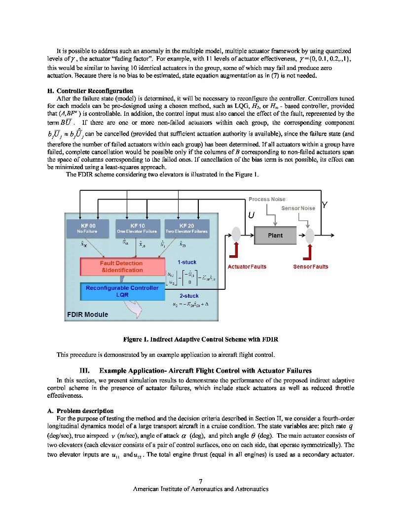
H. Controller ReconfigurationAfter the failure state (model) is determined, it will be necessary to reconfigure the controller. Controllers tuned

for each models can be pre-designed using a chosen method, such as LQG, H2, or H. - based controller, providedthat (A,BFa ) is controllable. In addition, the control input must also cancel the effect of the fault, represented by theterm B U . If there are one or more non-failed actuators within each group, the corresponding component

bjUj bjU

j can be cancelled (provided that sufficient actuation authority is available), since the failure state (and

therefore the number of failed actuators within each group) has been determined. If all actuators within a group havefailed, complete cancellation would be possible only if the columns of B corresponding to non-failed actuators spanthe space of columns corresponding to the failed ones. If cancellation of the bias term is not possible, its effect canbe minimized using a least-squares approach.

The FDIR scheme considering two elevators is illustrated in the Figure 1.

Figure 1. Indirect Adaptive Control Scheme with FDIR

This procedure is demonstrated by an example application to aircraft flight control.

III. Example Application- Aircraft Flight Control with Actuator FailuresIn this section, we present simulation results to demonstrate the performance of the proposed indirect adaptive

control scheme in the presence of actuator failures, which include stuck actuators as well as reduced throttleeffectiveness.

A. Problem descriptionFor the purpose of testing the method and the decision criteria described in Section II, we consider a fourth-order

longitudinal dynamics model of a large transport aircraft in a cruise condition. The state variables are: pitch rate q(deg/sec), true airspeed v (m/sec), angle of attack a (deg), and pitch angle B (deg). The main actuator consists oftwo elevators (each elevator consists of a pair of control surfaces, one on each side, that operate symmetrically). Thetwo elevator inputs are u 11

andu12 . The total engine thrust (equal in all engines) is used as a secondary actuator.


The individual engine thrusts have been aggregated to produce a single control input u2 . The nominal model(ignoring noise) is

.z Ax b 1 (u 11 u 12 ) b2 u 2 (17)y Cx

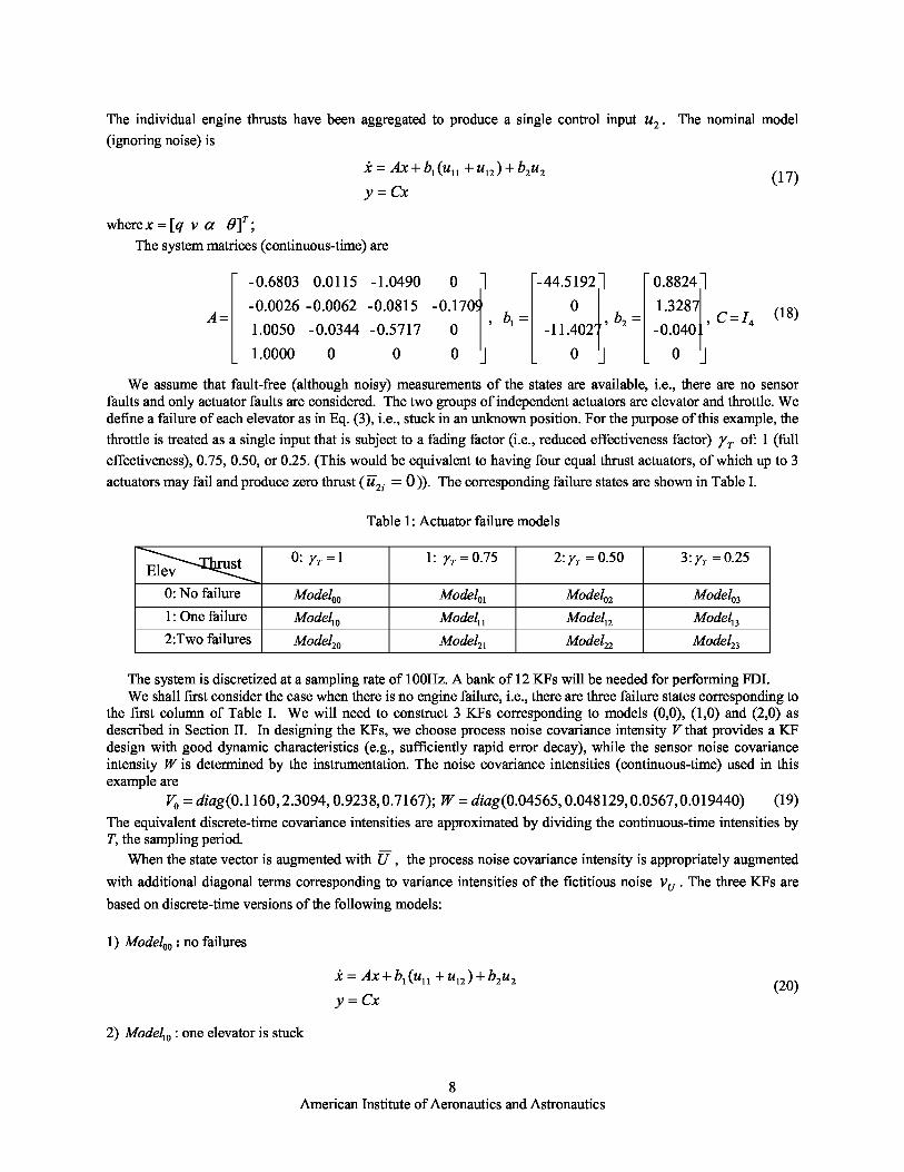
where x [q v ]T;The system matrices (continuous-time) are

- 0.6803 0.0115 -1.0490 0 -44.5192 0.8824 -0.0026 -0.0062 -0.0815 -0.17090 1.3287

A b b C I , 1 2 4 , , (18) 1.0050 -0.0344 -0.5717 0 -11.4027 -0.0401 1.0000 0 0 0 0 0

We assume that fault-free (although noisy) measurements of the states are available, i.e., there are no sensorfaults and only actuator faults are considered. The two groups of independent actuators are elevator and throttle. Wedefine a failure of each elevator as in Eq. (3), i.e., stuck in an unknown position. For the purpose of this example, thethrottle is treated as a single input that is subject to a fading factor (i.e., reduced effectiveness factor) T of: 1 (fulleffectiveness), 0.75, 0.50, or 0.25. (This would be equivalent to having four equal thrust actuators, of which up to 3actuators may fail and produce zero thrust ( u 2 i 0)). The corresponding failure states are shown in Table I.

Table 1: Actuator failure models

Elev st 0: T 1 1: T 0.75 2:T 0.50 3: T 0.25

0: No failure Model00 Model01 Model02 Model03

1: One failure Model10 Model11 Model12 Model13

2:Two failures Model20 Model21 Model22 Model23

The system is discretized at a sampling rate of 100Hz. A bank of 12 KFs will be needed for performing FDI.We shall first consider the case when there is no engine failure, i.e., there are three failure states corresponding to

the first column of Table I. We will need to construct 3 KFs corresponding to models (0,0), (1,0) and (2,0) asdescribed in Section II. In designing the KFs, we choose process noise covariance intensity V that provides a KFdesign with good dynamic characteristics (e.g., sufficiently rapid error decay), while the sensor noise covarianceintensity W is determined by the instrumentation. The noise covariance intensities (continuous-time) used in thisexample are

V0 diag(0.1160, 2.3094, 0.923 8,0.7167); W diag (0.04565, 0.048129, 0.0567, 0.019440) (19)

The equivalent discrete-time covariance intensities are approximated by dividing the continuous-time intensities byT, the sampling period.

When the state vector is augmented with U, the process noise covariance intensity is appropriately augmentedwith additional diagonal terms corresponding to variance intensities of the fictitious noise vU . The three KFs arebased on discrete-time versions of the following models:

1) Model00 : no failures

i Ax b1 (u 11 u 12 ) b2 u 2

(20)y Cx

2) Model10 : one elevator is stuck


In this case, one elevator (e.g., u 11 ) is stuck at a position u 11 . The state vector is augmented with u 11 :

x b 1 x

[b1

u 12 [b

2iu 2 (21)

u11

[A

00 C 1 1 0 0

3) Model20 : both the elevators are stuck.

x

u 1

C0 0 Cu 1

C0

2

u 2

(22)

Where:

u 1 u11 u 12

(23)

B. Elevator Failure Detection and Identification ResultsIt is assumed that the aircraft is in a cruise condition, with a nominal LQ state feedback control law. Suppose one

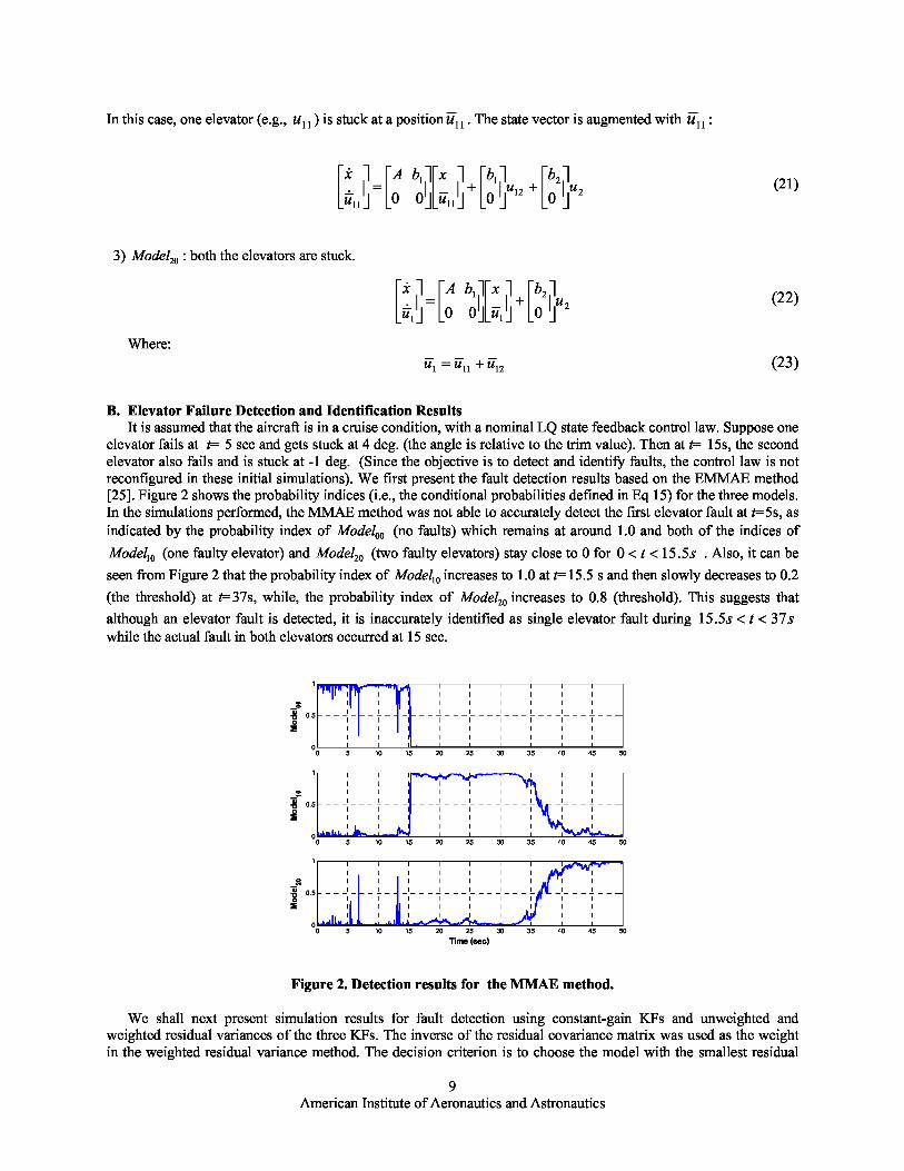
elevator fails at t= 5 sec and gets stuck at 4 deg. (the angle is relative to the trim value). Then at t= 15s, the secondelevator also fails and is stuck at -1 deg. (Since the objective is to detect and identify faults, the control law is notreconfigured in these initial simulations). We first present the fault detection results based on the EMMAE method[25]. Figure 2 shows the probability indices (i.e., the conditional probabilities defined in Eq 15) for the three models.In the simulations performed, the MMAE method was not able to accurately detect the first elevator fault at t= 5s, asindicated by the probability index of Model00 (no faults) which remains at around 1.0 and both of the indices ofModel10 (one faulty elevator) and Model20 (two faulty elevators) stay close to 0 for 0 t 15.5s . Also, it can beseen from Figure 2 that the probability index of Model10 increases to 1.0 at t= 15.5 s and then slowly decreases to 0.2(the threshold) at t= 37s, while, the probability index of Model20 increases to 0.8 (threshold). This suggests thatalthough an elevator fault is detected, it is inaccurately identified as single elevator fault during 15.5s t 37 swhile the actual fault in both elevators occurred at 15 sec.

1

I I I I I I I I

00.5

O9-- -

f I I I I I I I I I

I I I I I I I I

-- - -- - - - I - - - I - - - --

0I I I I I I I I I

0 5 10 15 20 25 30 35 40 45 50

1

I I I I I I I I

0

0.5 --

I

-II

I

II

I

II

II

I

II

I

II

I

II

I

II

I

II

0I I I I I I I

0 5 10 15 20 25 30 35 40 45 50

1

I I I I I I I I

n I I I I I I I I I

y 0.5

00 5 10 15 20 25 30 35 40 45 50

Time (sec)

Figure 2. Detection results for the MMAE method.

We shall next present simulation results for fault detection using constant-gain KFs and unweighted andweighted residual variances of the three KFs. The inverse of the residual covariance matrix was used as the weightin the weighted residual variance method. The decision criterion is to choose the model with the smallest residual


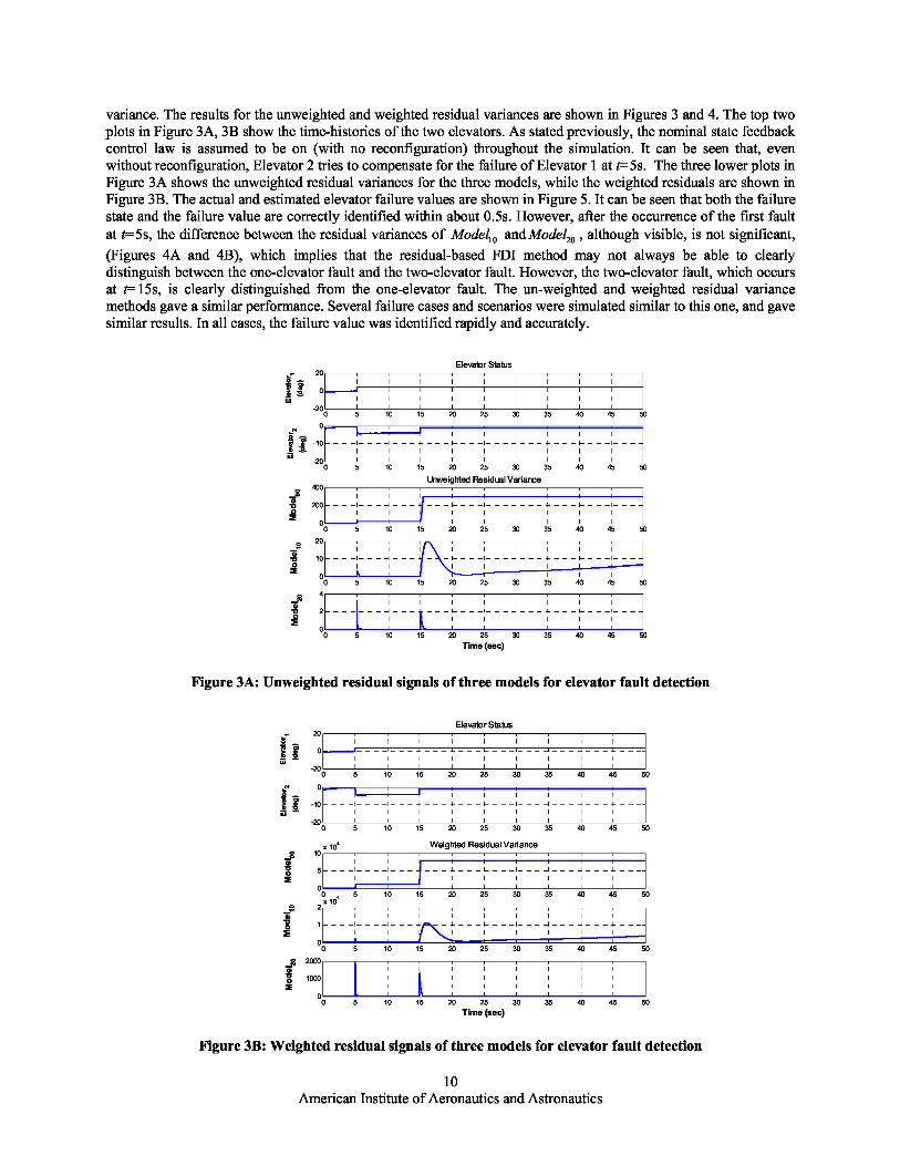
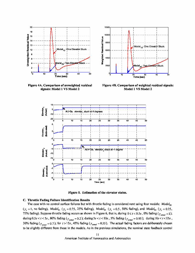
variance. The results for the unweighted and weighted residual variances are shown in Figures 3 and 4. The top twoplots in Figure 3A, 3B show the time-histories of the two elevators. As stated previously, the nominal state feedbackcontrol law is assumed to be on (with no reconfiguration) throughout the simulation. It can be seen that, evenwithout reconfiguration, Elevator 2 tries to compensate for the failure of Elevator 1 at t= 5s. The three lower plots inFigure 3A shows the unweighted residual variances for the three models, while the weighted residuals are shown inFigure 313. The actual and estimated elevator failure values are shown in Figure 5. It can be seen that both the failurestate and the failure value are correctly identified within about 0.5s. However, after the occurrence of the first faultat t= 5s, the difference between the residual variances of Model10 and Model20 , although visible, is not significant,(Figures 4A and 413), which implies that the residual-based FDI method may not always be able to clearlydistinguish between the one-elevator fault and the two-elevator fault. However, the two-elevator fault, which occursat t= 15s, is clearly distinguished from the one-elevator fault. The un-weighted and weighted residual variancemethods gave a similar performance. Several failure cases and scenarios were simulated similar to this one, and gavesimilar results. In all cases, the failure value was identified rapidly and accurately.

20Elevator Status

I- - - - - - - -I- - - - - - - - -I- - -a...._ 0 - - - - - - -

W

-200 5 10 15 20 25 30 35 40 45 50

0

-10v

W-20

I I I I I I I I I

0 5 10 15 20 25 30 35 40 45 50

400Unweighted Residual Variance

9 200 _ _ _I_ _ _ _ _ _ _ _ _ _ _ _I_ _ _ -4 _ _ _ 1gi

0I I I I

0 5 10 15 20 25 30 35 40 45 50

20I I

10 _ _ _I_ _ _ -4 _ _ _

1\LL

gi0

0 5 10 15 20 25 30 35 40 45 50

4

2I I I I I I I

00 5 10 15 20 25 30 35 40 45 50

Time (sec)

Figure 3A: Unweighted residual signals of three models for elevator fault detection

Elevator Status20

Q

0W

-200 5 10 15 20 25 30 35 40 45 50

0$ v

-10W I I I

-200 5 10 15 20 25 30 35 40 45 50

x 104 Weighted Residual Variance

10m I I

C 5 ___I____I___2

00x 10

45 10 15 20 25 30 35 40 45 50

2m I I I I I I I I I

1^

- - - - - - -I- -I I

- 4_ _ L

-- - -

I I I

--- - - -- - -

I I

- L _ _ _

I

00 5 10 15 20 25 30 35 40 45 50

2000I I I I I I I I

41

9p 1000- I ---I

- - - - - - - - -I- - -

I I I

- - - - -

I I

- - - -

I

00 5 10 15 20 25 30 35 40 45 50

Time (sec)

Figure 3B: Weighted residual signals of three models for elevator fault detection


5 10 15 20 25 30 35 40 45 50

0Ij

18 I ^ 1 I I I16

1 ;14

121

1 I10 - - - - - + - - a - T ^ Model 10 : One Elevator Stuck

8

1

61 ;

I 1 11 I I4 - - - - -- - i Model

20: Two Elevator Stuck - -

2 - - T1 IT'^—

00 10 20 30 40 5

Time (sec)

Figure 4A. Comparison of unweighted residualsignals: Model 1 VS Model 2

I I I I

I ^ I I II A.-

I I I10000 - - - - - -- - ------ -----

^ I I l I I I

8000

' I 1 1 I I I1 1

I , , I I I.a

Model 10 : ne Elevator StuckC1 r

6000 7-- -t- I - - - - - - r 7

4000

I ; 1 1 I IW , 1 1

w , 1 1^ I 1 , I I I Ì•m I ^ 1 I I

;I

2000 - - - - + - - y - - Model 20 : Two Elevator Stuck -

I ^ I

I I I I

00 10 20 30 40 50

Time (sec)

Figure 4B. Comparison of weighted residual signals:Model 1 VS Model 2

10

0

W -10

-200

5a

E0

m WW W

-50

0

N -5^ W

m-10

W

-150

0

N -2W

m w -4

W W

-60

At t=5s. elevator1 stuck at 4 degrees II I I I I I I I I

5 10 15 20 25 30 35 40 45 50

I

I R I I I I I IAt t=15s. elevator2 stuck at -1 degree - - ,

I I I I I I I I I

5 10 15 20 25 30 35 40 45 50

5 10 15 20 25 30 35 40 45 50Time (sec)

Figure 5. Estimation of the elevator status.

C. Throttle Fading Failure Identification ResultsThe case with no control surface failures but with throttle fading is considered next using four models: Model00

(y7,

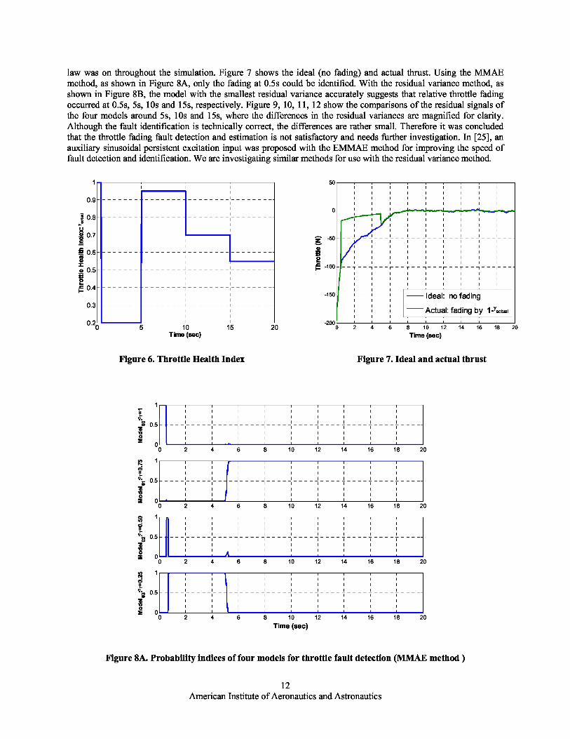
= 1, no fading), Model01 (y7, = 0.75 , 25% fading), Model02 (y7, = 0.5 , 50% fading), and Model03 (y7, = 0.25 ,75% fading). Suppose throttle fading occurs as shown in Figure 6, that is, during 0 !9 t < 0.5s , 0% fading (yactual = 1);

during 0.5s < t < 5s , 80% fading (yactual

= 0.2); during 5s < t < 10s , 5% fading (yactual

= 0.95); during 10s < t < 15s ,

30% fading (yactual

= 0.7); for t > 15s , 45% fading (yactual = 0.55). The actual fading factors are deliberately chosen

to be slightly different from those in the models. As in the previous simulations, the nominal state feedback control


0.s

0.8

0.7S

0.6Wm2m 0.5

H 0.4

0.3

law was on throughout the simulation. Figure 7 shows the ideal (no fading) and actual thrust. Using the MMAEmethod, as shown in Figure 8A, only the fading at 0.5s could be identified. With the residual variance method, asshown in Figure 8B, the model with the smallest residual variance accurately suggests that relative throttle fadingoccurred at 0.5s, 5s, 10s and 15s, respectively. Figure 9, 10, 11, 12 show the comparisons of the residual signals ofthe four models around 5s, 10s and 15s, where the differences in the residual variances are magnified for clarity.Although the fault identification is technically correct, the differences are rather small. Therefore it was concludedthat the throttle fading fault detection and estimation is not satisfactory and needs further investigation. In [25], anauxiliary sinusoidal persistent excitation input was proposed with the EMMAE method for improving the speed offault detection and identification. We are investigating similar methods for use with the residual variance method.

0- I -I I I I I I

I I I I I I I I I

I I I I I I I I I

I I I I I I I I

- ------------- - - - - - -- - -- - - - -Z -50 I I I I I I I I

^ I I I I I I I I I

I I I I I I I I I

p I I I I I I I I I

t -100

I I I I I I I I I

I I I I I I I I I

I I I I I I I I I

I I I

-150 + - - - Ideal: no fadingI I I

I I I

Actual: fading by 1-actual

I I

0.20 -2005 10 15 20 0 2 4 6 8 10 12 14 16 18 20

Time (sec) Time (sec)

Figure 6. Throttle Health Index Figure 7. Ideal and actual thrust

1II I I I I I I I I I4

I I I I I I I I I

o0^5 ---------------------------------------I^ I I I I I I I I I9o

00 2 4 6 8 10 12 14 16 18 20

In 1GIFS. 0.5om

II -

I- -

I --I

II

II-----------------------

II

II

II

I---I

II____--I

90

^ 0I I I I I I I I I

0 2 4 6 8 10 12 14 16 18 20

0 1N

cisSiV 0.5pm

I I I I I I I--

I-- --

I--

90^ 0

I I I I I I I I I

0 2 4 6 8 10 12 14 16 18 20

In 1NGIF

0.5p -----III

-I

--I--II

III

III

-----------------------III

III

III

I---I

I

II____--II

o

0I I I I I I I I I

0 2 4 6 8 10 12 14 16 18 20

Time (sec)

Figure 8A. Probability indices of four models for throttle fault detection (VIVIAE method )

I I I I I I I I I

I I I I I I I I I

I I I I I I I I I

I I I I I I I I I


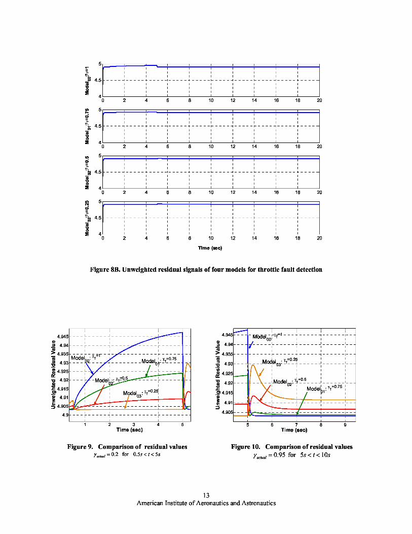
2 4 6 8 10 12 14 16 18 20

2 4 6 8 10 12 14 16 18 20

5nto

4.5mv0

40

10 5n0n

e4.5

dO

40

50n

Tg 4.5Zv0

40

u1 5NC11

tb 4.5

Zv0M 4

0

2 4 6 8 10 12 14 16 18 20

2 4 6 8 10 12 14 16 18 20

Time (sec)

Figure 8B. Unweighted residual signals of four models for throttle fault detection

4.945 - - - - - - - - - 1------------' ---- -d? 4.94 - - -i - - - - - - - - - - ----- i ----- -> 4.935 ---r- - =1--1- ----1------r----- -â Model

0 :

rT

Mr =0.75

493 - - - 0 - - - - - - - - - -- odet0 -T -- - -

d4.925 - - -- -- ------'--- --------=0 .54.92 - - - i -ModeF ^ yr = - - - - - - -- - - - - -,

x 4.915 -- r--- ^ -- - - - - i - - - _ 0.25------ -rn Model :r

T0 4.91-- - -- -- ---- -1-03 ---- -- - - -

- .3 i i

j4.905 Y ----- -4.9 - - - -- - - - -- - - - - I -- - - - - -

----- -I I I I I

1 2 3 4 5Time (sec)

Figure 9. Comparison of residual valuesractwal =0.2 for 0.5s < t <5s

4.945 - - - - Model-rrT

=1 - - - - - - - - - - - - - - - --

00I 1 1

3 4.94 - - - / - - - -- - - - - - I4.935 ---------r-----r-----7------r-

3 -Model :r

T=0.25

------------'--

v 4.93 - - - - - -

LI

iM

4.925 ----r-----7------r-=0.5d 4.92 - - - - - - - - - - - -'- -

-0.75---

s Model: r =

01 4.915 - - -

--- -- ^ 1 - T ---r-

c 4.91

4.905 ---- - - - - - - - - - - - - I--I

5 6 7 8 9Time (sec)

Figure 10. Comparison of residual valuesractwal =0.95 for 5s < t <10s


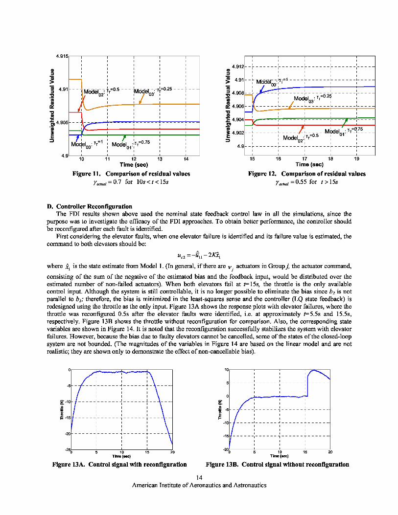
4.915

d3>

7 4.91

d

d

4.905RM

3c

4.9

I I I I I

I I I I I

I I I I I

I I I I I

I I I I I

I I I I I

I I I I

- - Model02

: yr=0.5 - - Model

03:

yr=0.25 - - - - -

6

I I I I

I I I

I I I I I

I I I I

I I I I

--- --- ------------------ - --

I I I I

I

I I I I

Model 00:

yr=1 Model

01:

yr=0.75

I I I I I

10 11 12 13 14Time (sec)

Figure 11. Comparison of residual valuesyactual

= 0.7 for 10s < t < 15s

I I I I I

4.912 -------- I - -- - - - - -- - - - - - - - - - - - - ----^ I I I I3 I I I I I

I I I I I

4.91 - ^ Model00

: yr= 1 ----

^ 4.908 ----, ------, - - - - - - - - - - --,----y k

Model yr= 0.2

1 1 03' 1

4.906 ------ L- - --- - L- - - - - - - - - - - - - - '----^ I I I I

t 4.904 ' ---r r------r--- - - 1----

Cm•3 1 1

_I I • y =0.753 4.902 _L______L____ L

-- -- -Model

1. r_1____-

0 .5 I

, Model : rr02

1 ,4.9

I I I I I

15 16 17 18 19Time (sec)

Figure 12. Comparison of residual valuesy

actual = 0.55 for t > 15s

D. Controller ReconfigurationThe FDI results shown above used the nominal state feedback control law in all the simulations, since the

purpose was to investigate the efficacy of the FDI approaches. To obtain better performance, the controller shouldbe reconfigured after each fault is identified.

First considering the elevator faults, when one elevator failure is identified and its failure value is estimated, thecommand to both elevators should be:

uc2 = —u11 — 2Kx

1

where xˆ1 is the state estimate from Model 1. (In general, if there are v

actuators in Group j, the actuator command,

consisting of the sum of the negative of the estimated bias and the feedback input, would be distributed over theestimated number of non-failed actuators). When both elevators fail at t= 15s, the throttle is the only availablecontrol input. Although the system is still controllable, it is no longer possible to eliminate the bias since b2 is notparallel to b1; therefore, the bias is minimized in the least-squares sense and the controller (LQ state feedback) isredesigned using the throttle as the only input. Figure 13A shows the response plots with elevator failures, where thethrottle was reconfigured 0.5s after the elevator faults were identified, i.e. at approximately t= 5.5s and 15.5s,respectively. Figure 13B shows the throttle without reconfiguration for comparison. Also, the corresponding statevariables are shown in Figure 14. It is noted that the reconfiguration successfully stabilizes the system with elevatorfailures. However, because the bias due to faulty elevators cannot be cancelled, some of the states of the closed-loopsystem are not bounded. (The magnitudes of the variables in Figure 14 are based on the linear model and are notrealistic; they are shown only to demonstrate the effect of non-cancellable bias).

Time (sec)

Time (sec)

Figure 13A. Control signal with reconfiguration Figure 13B. Control signal without reconfiguration


0

-20

-40

-60

-80

-100

-120

-140

-160

20

Velocity (m/s)I I

Pitch Rate (deg/s)- - - - -L -- - - - -

Pitch Angle (deg)

-------I-------1-------+ \-----I I I

, r

I I I

I I I +- _ _I I I `

Angle of Attack (deg)I I I

I I I

--------------II I I

I I I

40

I I I

I I I

30 - - - - - - - -I- - - - - - - -I- - - - - - - -I - - - - - - -I I I

I I I

I I I

I I I

20Velocity (m/s)

I I I

I I I

10 - -- - - - - - - - - Angle of Attack (deg) - -------

I Î I

I I

0' i I I

I / I I

eg/s)----Pitch Angle- - (deg)-- ----- --10

- ----I I I `

I I I ^Î I I

I I I-200 5 10 15 20 0 5 10 15 20Time (sec) Time (sec)

Units: Angle of attack (deg), pitch angle (deg); pitch rate (deg/s); velocity (m/s)

Figure 14A. State variables without reconfiguration Figure 14B. State variables with reconfiguration

Although this example used LQG-based reconfigurable controller designs, methods such as H2 and H controlcan be used.

IV. Sensor Fault Detection and Identification

This section addresses the sensor failure detection and estimation problem, which is the dual of the actuatorfailure problem addressed in Section II.

We shall first consider the case where unknown constant bias terms exist in the sensors.

A. Sensor BiasConsider the system

x Ax Bu 0

y Cx y w

(24)

where C has a full rank (i.e., no redundant sensors), Y E R l denotes an unknown bias. As in the case of stuck-actuator failures the sensor bias can be estimated by augmenting the unknown bias term y to the system dynamicsand designing a KBF. The augmented system is:

r7

LyJ

[0 00 77

[

B U v (25)

0

y [C Il ] w (26)

The following theorem gives a necessary and sufficient condition for identifiability of the sensor bias.Theorem 2. For the system in (24), the sensor bias y is identifiable if and only if ( C, A) is observable and A has noeigenvalue at the origin.Proof- The above system is observable if and only if

sI A 0

0 sIl n l for s = A (A), and s = 0 (27)

C Il

Since (C, A) is observable, the first n columns of the test matrix in (27) are linearly independent for all s. For s 00, the last m columns are independent of each other and of the first n columns, i.e., p = n+ l. At s=0,


— A 0 — A 0 I 0 — A 0 n + l if and only if A ^ 0 (28)

P C Il J

= P C Il J —C Il J

= P 0 Il

J= Y ()

Discrete-time implementation- As in the case of actuator failures, discrete-time formulation is used inimplementation. In this case the condition in Theorem 2 simply requires that the discretized “A” matrix has noeigenvalues at z=1.

An alternate method for sensor bias removal that is used in practice is to implement washout filters. Forexample, with a first-order washout filter, the filtered sensor output is given by

c sYf (s) = Gwo

(s )Y (s) = cs + 1 Y(s)

(29)

where c is the time constant. The drawbacks of a washout filter, however, are: i) along with the bias, it also removesthe zero-frequency (DC) component of the signal, ii) it introduces a phase lag, and iii) it introduces a non-minimum-phase zero. To maintain the minimality of the system and to avoid unstable pole-zero cancellation, the plant shouldnot have poles at the origin.

B. Sensor Outage and Bias- Multiple Redundant SensorsWe consider the case wherein multiple redundant sensors are available for each measurement. Suppose there are

l groups of sensors, wherein each ( ith) group consists of Ni identical sensors, i.e., the sensor output of the jth sensorwithin the ith group is

yij = ci x + yij + wig i = 1, l ; j = 1, , Ni (30)

where the overhead bar denotes the unknown bias term. Suppose the outputs of all sensors within each ( ith) groupare averaged to get the measurement Yi :

Ni

y=( 11Ni ) E y=jj , i =1, , l (31)j=1

Suppose some of the sensors within each group experience an outage, e.g., if the kth sensor in the ith group fails,its output is

yik = [0]x + y

ik + w

ik(32)

In the bias estimation approach, the problem is to i) determine how many sensors within each group have failed,and ii) estimate the total bias in Yi. Similar to the actuator failure case, this can be done by designing multiple KFs,each tuned to a different sensor failure model. For simplicity, consider the case with two groups of sensors whereinthe first group has 2 identical sensors and the second group has 3 identical sensors. The three possible sensor failurestates for Group 1 are: no outages, one outage, and two outages. Similarly there are 4 sensor failure states for Group2. Thus the outputs of the two groups are given by

C Y J = F s Cx + Y + w (33)

Y2 11

where Y is the effective bias vector and Fs is the sensor failure matrix which can take on 3x4= 12 values:

F s =['5

1

'52 '1, '51 = 1, 0.5, 0; '52 = 1, 0.667,0.333, 0 (34)

For the multiple model FDI method, the procedure is to augment the system dynamics as in (25), and to designl

12 KBFs, each tuned to one of the 12 sensor models. In general, there would be (Ni + 1) sensor failure statesi=1

including the no-failures and all-failures cases. As long as ( FsC, A) is observable (i.e., (C, A) is observable and atleast one sensor within each group is working) and A has no eigenvalues at the origin, it is possible to estimate the


bias and the state. As in the case of actuator failures, the model with the highest conditional probability or thesmallest residual norm determines the correct failure state. However, based on the experience with actuator failures,it may not be possible to make a clear distinction between similar sensor failure states.

We shall next consider the case of simultaneous actuator and sensor failures.

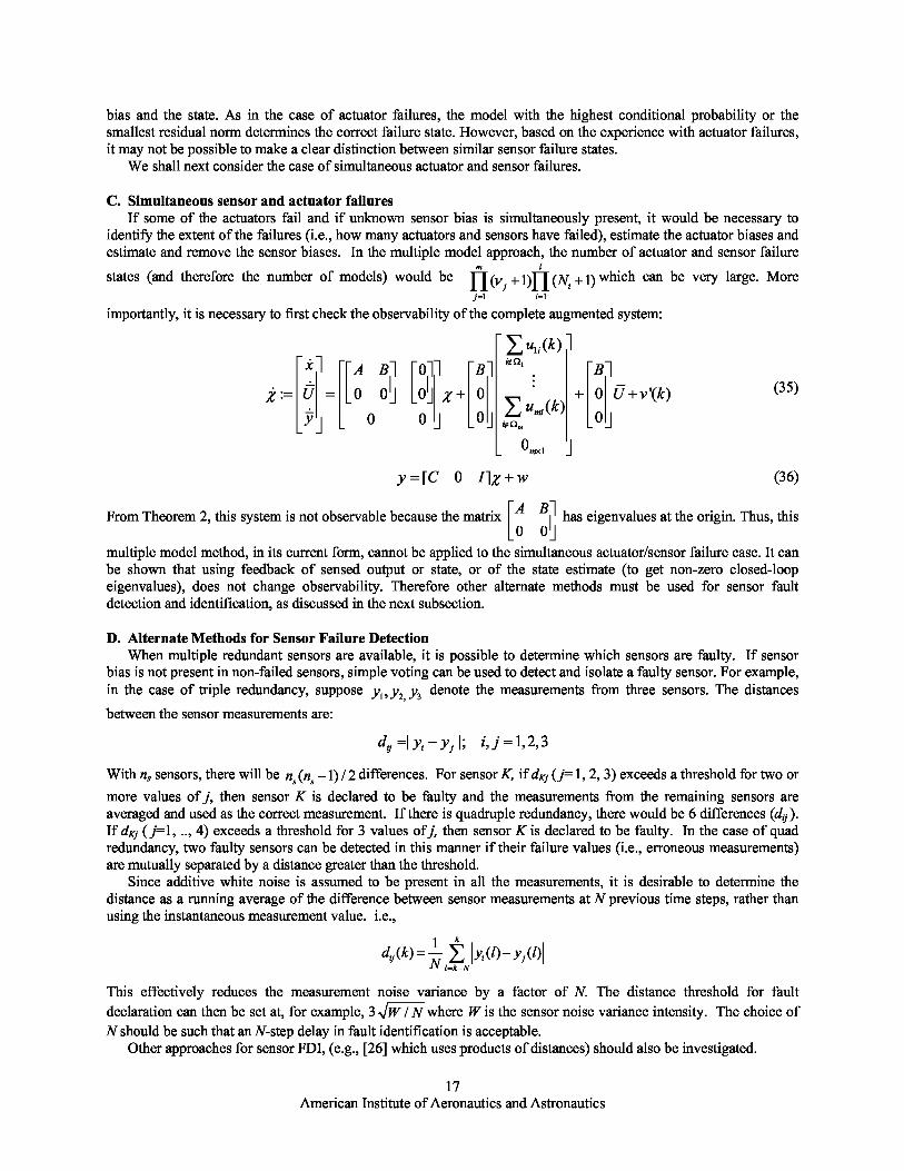
C. Simultaneous sensor and actuator failuresIf some of the actuators fail and if unknown sensor bias is simultaneously present, it would be necessary to

identify the extent of the failures (i.e., how many actuators and sensors have failed), estimate the actuator biases andestimate and remove the sensor biases. In the multiple model approach, the number of actuator and sensor failure

m l

states (and therefore the number of models) would be (j 1) (Ni 1) which can be very large. Morej 1 i1

importantly, it is necessary to first check the observability of the complete augmented system:

ujk) X A B 0B

B

: U [ 0 0 10 0 0

U v '(k) (35)

u ,^Z (k)y

0 0 J 0 im 0 0 ,^ 1

y [C 0 I ] w (36)

From Theorem 2, this system is not observable because the matrix A Bi has eigenvalues at the origin. Thus, this 0 0

multiple model method, in its current form, cannot be applied to the simultaneous actuator/sensor failure case. It canbe shown that using feedback of sensed output or state, or of the state estimate (to get non-zero closed-loopeigenvalues), does not change observability. Therefore other alternate methods must be used for sensor faultdetection and identification, as discussed in the next subsection.

D. Alternate Methods for Sensor Failure DetectionWhen multiple redundant sensors are available, it is possible to determine which sensors are faulty. If sensor

bias is not present in non-failed sensors, simple voting can be used to detect and isolate a faulty sensor. For example,in the case of triple redundancy, suppose

y1, y2, y3 denote the measurements from three sensors. The distances

between the sensor measurements are:

dij j yi yj j ; i, j 1, 2, 3

With ns sensors, there will be ns (ns 1) / 2 differences. For sensor K, if dKj ( j= 1, 2, 3) exceeds a threshold for two ormore values of j, then sensor K is declared to be faulty and the measurements from the remaining sensors areaveraged and used as the correct measurement. If there is quadruple redundancy, there would be 6 differences ( dij ).

If dKj ( j=1, .., 4) exceeds a threshold for 3 values of j, then sensor K is declared to be faulty. In the case of quadredundancy, two faulty sensors can be detected in this manner if their failure values (i.e., erroneous measurements)are mutually separated by a distance greater than the threshold.

Since additive white noise is assumed to be present in all the measurements, it is desirable to determine thedistance as a running average of the difference between sensor measurements at N previous time steps, rather thanusing the instantaneous measurement value. i.e.,

k1d k y l y l

ij ( ) ( ) ( )

i j

N l kN

This effectively reduces the measurement noise variance by a factor of N. The distance threshold for faultdeclaration can then be set at, for example, 3 W / N where W is the sensor noise variance intensity. The choice ofN should be such that an N-step delay in fault identification is acceptable.

Other approaches for sensor FDI, (e.g., [26] which uses products of distances) should also be investigated.


V. Concluding Remarks

An indirect adaptive control scheme based on multiple model methods was proposed. Actuator failure detectionand identification (FDI) for systems having groups of similar actuators was first addressed. The actuator failuretypes consisted of unknown actuators stuck in unknown positions, and reduced effectiveness (actuator fading). Theapproach uses a bank of Kalman filters based on multiple models, and subsequent control reconfiguration to mitigatethe effect of biases caused by failed actuators, as well as to obtain stability and satisfactory performance using theremaining actuators. Conditions for actuator fault identifiability were presented, and methods for controlreconfiguration were discussed. The scheme utilizes constant-gain Kalman filters and a residual-based decisioncriterion, which substantially reduces complexity and real-time computation needs. Results of application of thescheme to an aircraft flight control example indicate that actuator faults can be detected and estimated rapidly andaccurately, although some difficulty was observed in distinguishing between similar faults and in estimating theactuator fading factor. Use of persistent excitation to increase the information content offers promise in this regardand will be addressed in future work. The dual problem of sensor FDI for a class of sensor failures (sensor biasesand outages) was also addressed, and conditions for sensor fault identifiability were presented. It was shown that itis not possible to estimate simultaneous actuator and sensor bias faults, and therefore alternate methods for sensorFDI need to be investigated. A brief discussion of sensor FDI using multiple redundant sensors was presented. Thefocus of this paper was on FDI; therefore the system parameters were assumed to be known. Future research isplanned for incorporating real-time system identification in conjunction with fault detection and estimation.

References

1 G. Tao, S. Chen, X. Tang, and S. M. Joshi, Adaptive Control of Systems With Actuator Failures, Springer-Verlag, London,2004.

2Gang Tao, Suresh M. Joshi, “Direct Adaptive Control of Systems with Actuator Failures: State of the Art and ContinuingChallenges,” AIAA Guidance, Navigation, and Control Conference , 2008, manuscript .

3Gang Tao, Suresh M. Joshi, and Xiaoli Ma, “Adaptive State Feedback and Tracking Control of Systems with ActuatorFailures,” IEEE Trans. Automatic Control, Vol. 46, No. 1, 2001, pp. 78-95,

4Xidong Tang, Gang Tao and Suresh M. Joshi, “Adaptive Actuator Failure Compensation for Nonlinear MIMO Systems withAn Aircraft Control Application,” Automatica, Vol. 43, No. 11, 2007, pp. 1869-1883.

5K. S. Kim, K. J. Lee, and Y. D. Kim, “Reconfigurable Flight Control System Design Using Direct Adaptive Method,” J.Guidance, Control, and Dynamics, Vol. 26, No. 4, 2003, pp. 543-550.

6W. D. Morse, and K. A. Ossman, “Model Following Reconfigurable Flight Control Systems for the AFTI/F-16,” J.Guidance, Control, and Dynamics, Vol. 13, No. 6, 1990, pp. 969-976.

7P. S. Maybeck, and R. D. Stevens, “Reconfigurable Flight control via Multiple Model Adaptive Control Methods,” IEEETrans. Aero. and Elect. Syst., Vol. 27, No. 3, 1991, pp.470-479.

8Youmin Zhang, and Jin Jiang, “Bibliographical Review on Reconfigurable Fault-Tolerant Control Systems,” Proc. 5th IFACSymfosium on Fault Detection, Supervision and Safety for Technical Processes, Washington, D. C. , June 2003, pp. 265-276.

D. D. Moerder, N. Halyo, J. R. Broussard, and A. K. Caglayan, “Application of Precomputed Control Laws in aReconfigurable Aircraft Flight Control System,” J. Guidance, Control and Dynamics, Vol. 12, No. 3, 1989, pp. 325-333.

10J. Jiang, “Design of Reconfigurable Control Systems Using Eigenstructure Assignment,” Int. J. Control, Vol. 59, No. 2,1994, pp. 395-410.

11Youming Zhang, and Jin Jiang, “Integrated Active Fault-Tolerant Control Using IMM Approach,” IEEE Trans. Aerosp.Elect. Syst., Vol. 37, No. 4, 2001, pp. 1221-1235.

12Y. Z. Gao, and P. J. Antsaklis, “Stability of the Pseudo-Inverse Method for Reconfigurable Control System,” Int. J.Control, Vol. 53, No.3, 1991, pp. 717-729.

13JL.-W. Ho, and G. G. Yen, “Reconfigurable Control System Design for Fault Diagnosis and Accommodation,” Int. J.Neural Systems, Vol. 12, No. 6, 2002, pp. 497-520.

14J. Chen, and R. J. Patton, Robust Model-Based Fault Diagnosis for Dynamic Systems, Boston, MA: Kluwer, 1999.15Saeid Habibi, “Parameter Estimation Using a Combined Variable Structure and Kalman Filtering Approach,” J. Dynamic

Systems, Measurement, and Control, Vol. 130, No. 5, 2008, pp. 051004-1-051004-14.16F. Caccavale, F. Pierri, and L. villain, “Adaptive Observer for Fault Diagnosis in Nonlinear Discrete-Time Systems,” J.

Dynamic Systems, Measurement, and Control, Vol. 130, No. 2, 2008, pp. 021005-1-021005-14.17Jianhui Luo, and Krishna R. Pattipati, “Agent-based Real-time Fault Diagnosis,” Aerospace, 2005 IEEE Conference, Big

Sky, MT, 2005, pp. 3632-3640.18Wen Chen, and Fahmida N. chowdhury, “Analysis and Detection of Incipient Faults in Post-Fault Systems Subject to

Adaptive Fault-Tolerant Control,” Int. J. Adaptive Control and Signal Processing, 2008, Vol. 22, No. 9, pp. 815-832.AdaptiveWang and Kai-Yew Lum, “Adaptive Unknown Input Observer Approach for Aircraft Actuator Fault detection and

Isolation,” Int. J. Adaptive Control and Signal Processing, 2007, Vol. 21, No. 1, pp. 31-48.


20M. Athans, D. Castanon, K. Dunn, C. S. Greene, W. H. Lee, and N. R. Sandell, Jr., “The Stochastic Control of the F-8CAircraft using a Multiple Model Adaptive Control (MMAC) Method- Part I: Equilibrium Flight,” IEEE Trans. AutomaticControl, Vol. AC-22, No. 5, 1977, pp 768-780.

21Peter S. Maybeck, “Multiple Model Adaptive Algorithms for Detecting and Compensating Sensor and Actuator/SurfaceFailures in Aircraft Flight Control Systems,” Int. J. Robust and Nonlinear Control, Vol. 9, 1999, pp. 1051-1070.

22Menke T., and Maybeck, P. S., “Sensor/Actuator Failure Detection in the Vista F-16 by Multiple Model AdaptiveEstimation,” IEEE Trans on Aerospace & Electronics Systems, Vol. 31, No. 4, 1995, pp. 1218-1228.

23Kumpati S. Narendra, and Jeyendran Balakrishnan, “Adaptive Control Using Multiple Models,” IEEE Trans. AutomaticControl, Vol. 42, No. 2, 1997, pp. 171-187.

24Jovan D. BoÏskovic and Raman K. Mehra, “Multiple-Model Adaptive Flight Control Scheme for Accommodation ofActuator Failures,” J. Guidance, Control, and Dynamics, Vol. 25, No. 4, 2002, pp. 712-724.

25P G. Ducard, H. P. Geering, “Efficient Nonlinear Actuator Fault Detection and Isolation System for Unmanned AerialVehicles,” J. Guidance, Control, and Dynamics, Vol. 31, No. 1, 2008, pp. 225-237.

26J. Ackermann, “Robustness Against Sensor Failures,” Automatica, Vol. 20, No. 2, 1984, pp. 211-215.


Documents

An Indirect Adaptive Control Scheme in the Presence of ... · An Indirect Adaptive Control Scheme in the ... (less than a second) ... We propose an indirect adaptive control scheme