The Pennsylvania State University APPLIED RESEARCH LAB

P.O. Box 30 State College, PA 16804

An Independent Component Analysis Blind Beamformer

by

Marc L. Salerno

Technical Report No. TR 00-007 December 2000

Supported by: L.R. Hettche, Director Office of Naval Research Applied Research Laboratory

Approved for public release, distribution unlimited

20001207 161

1. AttNCT UM OMIT (U*W Bttnftj 12. RffORT DATI December 2000 Thesis in Electrical Engineering

4. TITU AND SUSTTTU

In Independent Component Analysis Blind Beamformer

C AUTHORS)

Marc L. Salerno

7. PfRfORMNJG ORGANIZATION NAMC(S) ANO AOMfSS<!S)

Applied Research Laboratory The Pennsylvania State University PO Box 30 State College, PA 16804

% SPONSORING/MONITOR*« AGENCY NAMI(S) ANO AOORJSSKSf

Office of Naval Research Ballston Tower 800 North Quincy St. Arlington, VA 22217 Mr. Les Jacobi

11. SUffUMfNTARY NOTIS

*. MRfORMNIO ORGANIZATION RlfORT NURMIR

TR 00-007

1«. SRONSORM« / MONITORS»« A«I NCV RtfORT NUMMI

12«. OrSTRRMjTKM/AVAlARRJTY STATIMINT

Approved for public release: distribution unlimited

12b. OtSTRRMJTION cooc

13. AlSTRAa (MMrnumJOOwonft)

Independent Component Analysis (ICA) has been proven to be a very successful method for separating mixed signals blindly. ICA works by using the assumption mat signal mixtures are combinations of independent signals. Up to now, ICA has been primarily used to separate signals where multiple amplitude combinations of these signals exist. The most popular of these ICA methods is Blind Source Separation (BSS). This thesis will expand on this to use the theory of ICA to separate mixed signals that are mixed by a beamformer. A new algorithm will be developed mat combines BSS and a new blind beamforming method to provide an estimate of the original unmixed signals and simultaneously learns their corresponding directions. This will all be performed without using any a priori knowledge about the source waveforms or their directions.

Results from mis algorithm were very promising and worked to separate multiple unknown signals that propagated from different unknown directions. Signal to Noise and Interference Ratios (SNIR) of the estimated signals, were found to significantly improve using this algorithm along with accurate estimates of their directions. BSS was also used in the algorithm to speed up convergence time and provide cleaner versions of the estimated signals. This algorithm was also shown to work well for wideband signals by using wideband network.

14. SUSMCT TtRMS

Beamforming, ICA,BSS, Blind Source Separation, Adaptive Algorithms, Nonlinear Adaptive Algorithms, Independent Component Analysis, Direction Estimation

IS. NUMUR Of M«S 68

it. ma coot

17. SICURffY CLASSIFICATION Of RtfORT

UNCLASSIFIED

It. SICUWTY OASSWCATION Of TWSFAOI

UNCLASSIFIED

1». SKUmrr OASS9KAT1Ö* Of ABSTRACT

UNCLASSIFIED

20. URNTATION Of ARSTRACT

NSN 7540-01-2RO-5SOO Standard Form 29« <R«v 2-89) f inntrt By AN« St« iJ*H JJfclM.

Abstract

Independent Component Analysis (ICA) has been proven to be a very successful

method for separating mixed signals blindly. ICA works by using the assumption that

signal mixtures are combinations of independent signals. Up to now, ICA has been

primarily used to separate signals where multiple amplitude combinations of these signals

exist. The most popular of these ICA methods is Blind Source Separation (BSS). This

thesis will expand on this to use the theory of ICA to separate mixed signals that are

mixed by a beamformer. A new algorithm will be developed that combines BSS and a

new blind beamforming method to provide an estimate of the original unmixed signals

and simultaneously learns their corresponding directions. This will all be performed

without using any a priori knowledge about the source waveforms or their directions.

Results from this algorithm were very promising and worked to separate multiple

unknown signals that propagated from different unknown directions. Signal to Noise and

Interference Ratios (SNIR) of the estimated signals, were found to significantly improve

using this algorithm along with accurate estimates of their directions. BSS was also used

in the algorithm to speed up convergence time and provide cleaner versions of the

estimated signals. This algorithm was also shown to work well for wideband signals by

using wideband network

ui

Table of Contents

List of Figures vj List of Tables viii Acknowledgements ix

1. Introduction 1

1.1 The Problem 1 1.2 Traditional Approaches 2 1.3 Thesis Overview 4

2. Background 5

2.1 Overview 5 2.2 Arrays and Beamformers 5

2.2.1 Representation of Array Inputs and Outputs 6 2.2.2 Beamformers 8

2.3 Adaptive Beamforming 11 2.3.1 The LMS Adaptive Beamformer 12 2.3.2 Constraints 15

2.4 Blind Beamforming 16 2.4.1 Cyclostationarity 17 2.4.2 Constant Modulus 17 2.4.3 The JADE Algorithm 18 2.4.3 Power Maximization Techniques 19

2.5 Other Methods 23 2.5.1 Blind Source Separation 23 2.5.2 Combination of Beamforming and a BSS 25

3. ICA Blind Beamforming 27

3.1 Overview 27 3.2 ICA Blind Beamformer 27

3.2.1 Independence Technique 27 3.2.2 Direction Estimation Using BSS 32 3.2.3 Combination of Independence and Direction Estimation

Techniques 35 3.2.4 Step Size Parameter Control 38

IV

3.3 Wideband Independence Based Blind Beamformer 40 3.3.1 The Array 41 3.3.2 The Bandpass Network 42 3.3.3 The Blind Beamformers 43 3.3.4 The Reconstruction Network 43 3.3.5 The Direction Estimator 44

4. Simulations and Results 45

4.1 Overview 45 4.2 Simulations 45

4.2.1 Simulations With and Without Step Size Parameter Control 45 4.2.2 Additional Simulations 50 4.2.3 Angle Spacing Effects on Separation 55 4.2.4 Performance for Sources with Unequal Power Levels 56 4.2.5 Performance with Additive Noise 57 4.2.6 Simulation for Wideband Signals .....' 59

4.3 Conclusions 63

5. Conclusions and Future Work 64

5.1 Future Work 5.2 Conclusions. 5.1 Future Work 64

65

References ,,

List of Figures

Figure 2.1 iV-element Array with K Sources 7

Figure 2.2 Time Delay Beamformer 9

Figure 2.3 Wideband Beamformer with Tap-Delay Line 11

Figure 2.4 Adaptive Beamformer 13

Figure 2.5 Block Diagram For BSS 25

Figure 3.1 Block Diagram of ICA Blind Beamformer for Two Beams Using a N-element Array 37

Figure 3.2 Wideband Blind Beamformer Network 41

Figure 3.3 Wideband Array for N=3 and for 3 Frequency Bins 42

Figure 4.1 Fixed Beam Pattern for a Three-Element Array 46

Figure 4.2 Learning Curves for the (a) Simulations 1 (b) Simulation 2 47

Figure 4.3 Plot of SIR for (a) Beam 1 and (b) Beam 2 for Simulation 2 49

Figure 4.4 Step Size Parameter, jui(n), for Simulation 1 and Simulation 2. . . . 50

Figure 4.5 (a) Learning Curves and (b) Step Size Parameter, ßi{n), for Simulation 3 51

Figure 4.6 Plot of SIR for (a) Beam 1 and (b) Beam 2 for Simulation 3 52

Figure 4.7 Beam Patterns for (a) Beam 1 and (b) Beam 2 52

Figure 4.8 Fixed Beam Pattern for a Five-Element Array 53

Figure 4.9 Learning Curve for Three-Source Simulation 54

Figure 4.10 (a) Plot of an Array Element, (b) Plot of the Estimated Source and (c) Plot of Actual Source 55

Figure 4.11 SIR of the Output from Beam 1 vs. the Angle Separation of the Sources 56

vi

Figure 4.12 (a) SIR Improvement over Original SIR and (b) Estimated Angles for Source at +14° Over Original SIR 57

Figure 4.13 (a) SIR between Opposing Signals vs. Additive Noise Levels and (b) SNIR of Estimated Signals vs. Additive Noise Levels 58

Figure 4.14 (a) Linear Cross Correlation of Actual Sources and BSS Outputs, (b) Nonlinear Cross Correlation of Actual Sources and BSS Outputs, (c) Nonlinear Cross Correlation Between the Actual and Estimated Noise Source and (d) Nonlinear Cross Correlation Between the Actual and Estimated Communication Signal 61

Figure 4.15 Bit Error Plots for (a) No Processing, (b) Outputs From the Beamformers and (c) Outputs From the BSS Algorithm 62

VI1

List of Tables

Table 4.1 Setup for Wideband Simulation 59

Table 4.2 Results From Wideband Network 60

Table 4.3 SNIR for Algorithms With and Without BSS 60

vni

Acknowledgments

I would like to give special thanks to my advisor, Dr. Leon Sibul for all of his

help and guidance. I would also like to thank my co advisors, Dr. Nirmal Bose and Dr.

John Doherty, for their help and feedback. Special thanks to JeffCarvalho, Michael

Popkowski, and my sister, Amy, for their help in retrieving books needed for this thesis

and to my family, my fiance, the Popkowskis, and my friends for all of their support.

This material is based upon work supported by Mr. Les Jacobi, Code 333, the

Office of Naval Research, through the Naval Sea Systems Command under contract No.

N000-39-97-D-0042, Delivery Order No. 104.

IX

Chapter 1. Introduction and Overview

1.1 The Problem

In underwater environments, boats, machinery, sea life and other environmental

sources generate many acoustic signals. Depending on the listener, some of these passive

sounds may be important and some not. For example, it may be desirable to listen to boat

or machinery noise in which the environmental noise needs to be suppressed.

Environmental scientists may want to remove the boat and machinery noise to listen to

environmental noise. Whichever the case, the listener must remove the unwanted signals

from the mixture in order to get a good estimation of the signal emitted from the desired

source. In this same application it may also be desirable to find the direction of the

source along with an estimate of the signal waveform.

All of the above applications are concerned with passive sources, which means

that no a priori knowledge of the signal waveform and their directions are available.

Without this a priori knowledge, the signals themselves and their directions are not

known. The spectral characteristics may not be known. The only assumption that can be

made in order to separate the signals is that they are statistically independent.

The problem that this thesis will address is to separate multiple sources that are

naturally mixed as they impinge upon an array. This thesis will focus on separating

signals from unknown far-field mixtures and finding their corresponding directions by

using the properties of Independent Component Analysis assuming the number of sources

is known. No a priori knowledge of the sources waveforms and their directions will be

used.

1

1.2 Traditional Approaches

In underwater environments, the most common approach to removing unwanted

signals from mixtures is the use of beamforming and filtering. Filtering is ineffective if

the unwanted interference spectrum coincides with the desired signal spectrum.

Beamforming can separate signals that have coinciding power spectrums, but propagate

from different directions. Beamforming works by using an array or a group of listening

elements as a spatial filter. This method is efficient in suppressing unwanted noise

signals that arrive from different directions and separating directional signals from non-

directional signals. In some situations, the desired signal, whose direction is known, is

mixed with noise signals whose directions are unknown. Many algorithms have been

developed that use adaptive signal processing to find and remove the effect of these

unwanted noise signals. Most of these adaptive algorithms use a priori knowledge about

the desired signal and its location in order to accomplish this [1-4].

A recent method for separating mixtures of signals is known as Independent

Component Analysis (ICA). ICA is an extension of Principal Component Analysis

(PCA). While PCA minimizes the correlation between components, ICA works to make

the components statistically independent. Since independence is a much stronger

criterion that correlation, sources can be separated as long as they are statistically

independent [5]. Blind Source Separation (BSS) has been the most promising application

of ICA, in which signals are separated by using higher order statistical moments or

Information Theoretic criteria. Unlike filtering, BSS can separate signals that have

coinciding power spectrums but have different higher order spectra (polyspectra). So far

these algorithms work well in separating mixtures of signals; however, they give no

information about the location of the individual sources.

Recently, blind beamforming techniques have been developed to suppress these

unwanted noise signals without using any a priori knowledge of the desired signal's

location. However, most of these blind beamforming techniques were designed for use

with digital communications. These algorithms exploit different assumptions that are

only applicable to communication signals [1-4]. In many applications, such as passive

sonar, the desired signal does not satisfy the assumptions of communication signals, in

particular, no a priori knowledge of the signal waveform or class of signals is available.

Communication signals tend to be constant modulus (constant envelopes) and also tend to

be cyclostationary, which is defined as having periodic statistical averages [5]. Sonar

signals do not have these properties and have arbitrary amplitudes and widely varying

power levels. Some algorithms have been developed to learn the direction of sources by

adjusting the location of the main beam until the power of the output is maximized.

Unfortunately, this algorithm only works for finding the direction of a desired source that

has more power than the background noise. It can also be used to remove the effects of a

high power source so that the lower power sources can be found. These algorithms, in

general, are not designed to separate similar power signals from far field mixtures. Other

algorithms have also been developed to separate these unknown signals by using a

combination of beamforming and BSS; however, the directions of the sources still remain

unknown.

1.3 Thesis Overview

This thesis is split up into multiple parts. Chapter 2 is a background chapter that

presents information about existing techniques. This background chapter will review the

history and major concepts of arrays, beamforming and some traditional adaptive

beamforming algorithms. Current blind beamforming algorithms and BSS techniques

will also be introduced and discussed. Chapter 3 introduces the new ICA blind

beamforming algorithm that is based on statistical independence for both narrowband and

wideband signals. Chapter 4 presents simulations and results from the use of the

algorithm. The final chapter will deal with future work in this field and conclusions.

Chapter 2. Background

2.1 Overview

This chapter presents a review of traditional methods that are used in array

processing and source separation. This chapter starts out with a review of arrays and

beamformers. Adaptive beamforming and blind beamforming methods are also

introduced and discussed. This chapter ends with the introduction and review of current

BSS techniques. These reviews will give the mathematical framework for the ICA blind

beamformer to be presented in Chapter 3.

2.2 Arrays and Beamformers

Beamforming is one of the most common methods used to locate the directions of

sources in both acoustic and electromagnetic wave propagation. It is also a powerful tool

in removing unwanted noise sources that are located in directions other than the direction

of the desired source. Beamforming in acoustics date back to before World War I [6].

Before technology was developed to handle the signal processing for beamforming, the

human brain was used. Today beamforming is generally done in discrete-time with

electronics and computers.

The oldest and simplest method of beamforming is known as time-delay

beamforming. As technology grew, it became just as easy to implement phase shifts for

beamformers, which became the preferred method in beamforming for many adaptive

algorithms. Phase shifts are commonly used because many applications have been

written for communications in which the signals tend to be narrowband. Array

processing has become a large and substantial field in which many modern techniques are

being developed. Some of these modern techniques include beamforming in the

frequency domain and eigenvalue analysis [7]. This section will concentrate on time-

delay beamforming in order to lay out the concepts and mathematics needed for the ICA

Blind Beamformer.

2.2.1 Representation of Array Inputs and Outputs

In order to accomplish spatial filtering, either directional elements or an array can

be used. For the purposes of this paper, arrays will be used since the directionality can be

changed without any physical changes to the listening or transmitting devices. An array

consists of a group of listening or transmitting elements that are positioned at different

locations in space. The rest of this thesis will concentrate on arrays with omni-directional

listening elements. In the case for acoustics, the elements can be hydrophones,

microphones, accelerometers, ect. Antennas of all forms are generally used for

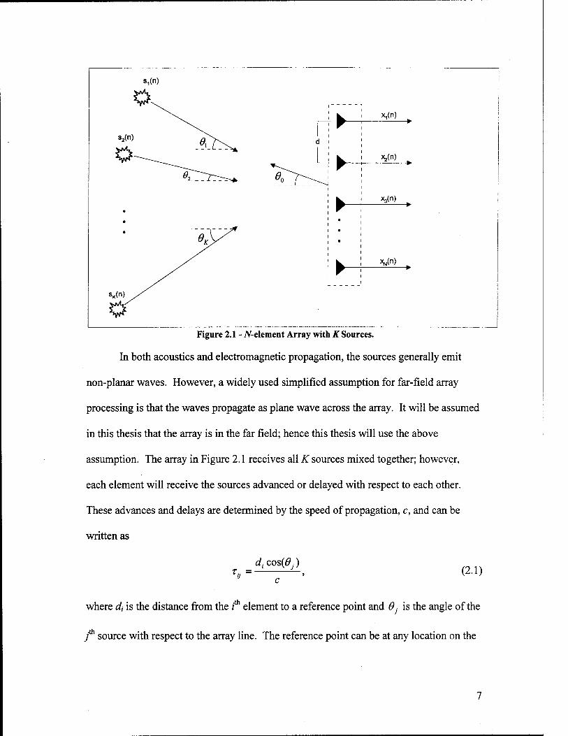
electromagnetic waves. Figure 2.1 shows a linear array that has N elements spaced an

equal distance apart, d, on the same axis with K sources impinging on it. The parameters

9x,92...9k are the angles between source positions and the perpendicular axis of the

array. The other parameter, 0O, is the steering angle that will be discussed in the next

section.

li t x,(n)

r

t x,(n)

r

Xs(n)

r m

a

m

XN(")

r

Figure 2.1 - iV-element Array with K Sources.

In both acoustics and electromagnetic propagation, the sources generally emit

non-planar waves. However, a widely used simplified assumption for far-field array

processing is that the waves propagate as plane wave across the array. It will be assumed

in this thesis that the array is in the far field; hence this thesis will use the above

assumption. The array in Figure 2.1 receives all K sources mixed together; however,

each element will receive the sources advanced or delayed with respect to each other.

These advances and delays are determined by the speed of propagation, c, and can be

written as

Tu = 4cos(0y)

(2.1)

where dt is the distance from the / element to a reference point and 9} is the angle of the

7th source with respect to the array line. The reference point can be at any location on the

array and is usually set to the center of the array. Each element of the array will now

have a combination of all the sources and can be written as

K

xl(n) = YjsJ(n-Tij) + nl(n), (2.2) 7=1

where n,(«) is additive noise added to the z* element which is statistically independent

with all sources and between elements. It should also be noted that for narrowband

signals (j-«1), Equation 2.2 can be written with phase shifts instead of time shifts,

which can make the math easier for some applications.

7=1 7=1 V + n» (2.3)

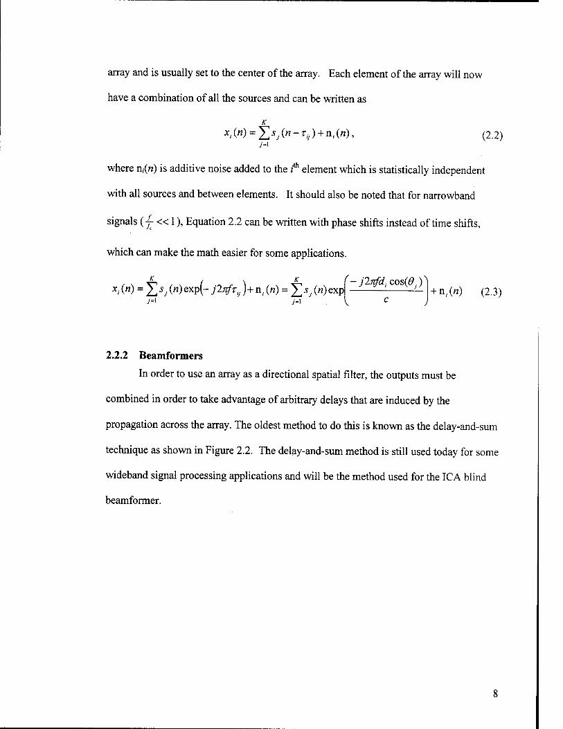
2.2.2 Beamformers

In order to use an array as a directional spatial filter, the outputs must be

combined in order to take advantage of arbitrary delays that are induced by the

propagation across the array. The oldest method to do this is known as the delay-and-sum

technique as shown in Figure 2.2. The delay-and-sum method is still used today for some

wideband signal processing applications and will be the method used for the ICA blind

beamformer.

w1 Z-T1

w2 Z-T2

^ W3

Z-T3 ^ ■

• •

WN z™ -

SUM Beamformer

Output

Figure 2.2 - Time Delay Beamformer.

This method works by adding delays to the elements of the beamformer in order to undo

the delays that are induced on the array from directional sources. The output of the

beamformer can be written as

X») = 2>Axt(»-7X*)), (2.4) *=i

where T is the time delay and w* is an element weight that is used for beam shading,

which can be used to change the beam shape. For purposes of this paper, all of the

weights will be equal and set to jj, so that the output of the array will have roughly the

same amplitude as the input. The time delays are chosen in order to steer the main beam

and are found by

T(k) = = (k-l)dsm(0o)/^ (2.5)

where 60 is the desired steering angle perpendicular to the array line as shown in Figure

2.1.

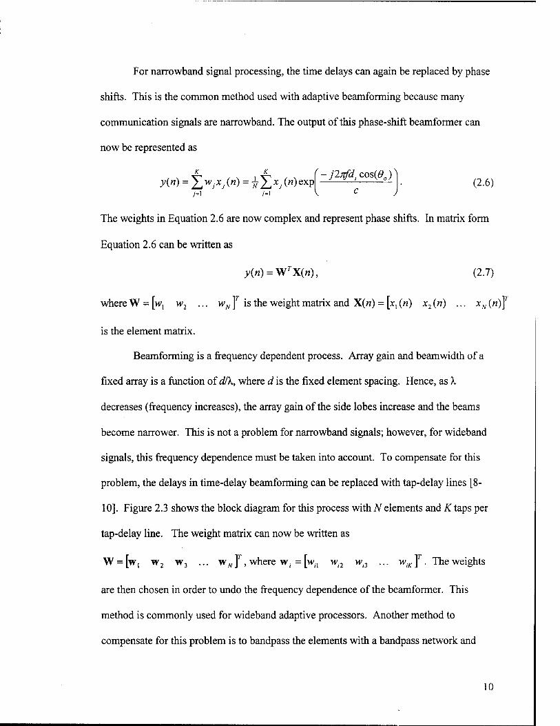
For narrowband signal processing, the time delays can again be replaced by phase

shifts. This is the common method used with adaptive beamforming because many

communication signals are narrowband. The output of this phase-shift beamformer can

now be represented as

y(n) = ]T WJXJ (») = ^ X XJ (") exP j=\ j=\

■j2nfdtcos{60) (2.6)

The weights in Equation 2.6 are now complex and represent phase shifts. In matrix form

Equation 2.6 can be written as

y(n) = VtTX(n), (2.7)

where W = [w, w2 ... wN J is the weight matrix and X(n) = [x{(n) x2(«) ... xN(w)f

is the element matrix.

Beamforming is a frequency dependent process. Array gain and beamwidth of a

fixed array is a function ofd/X, where d is the fixed element spacing. Hence, as X

decreases (frequency increases), the array gain of the side lobes increase and the beams

become narrower. This is not a problem for narrowband signals; however, for wideband

signals, this frequency dependence must be taken into account. To compensate for this

problem, the delays in time-delay beamforming can be replaced with tap-delay lines [8-

10]. Figure 2.3 shows the block diagram for this process with JV elements and K taps per

tap-delay line. The weight matrix can now be written as

W = [wj w2 w3 ... WJVJ", where w, =[w(1 wi2 wi3 ... wiKJ. The weights

are then chosen in order to undo the frequency dependence of the beamformer. This

method is commonly used for wideband adaptive processors. Another method to

compensate for this problem is to bandpass the elements with a bandpass network and

10

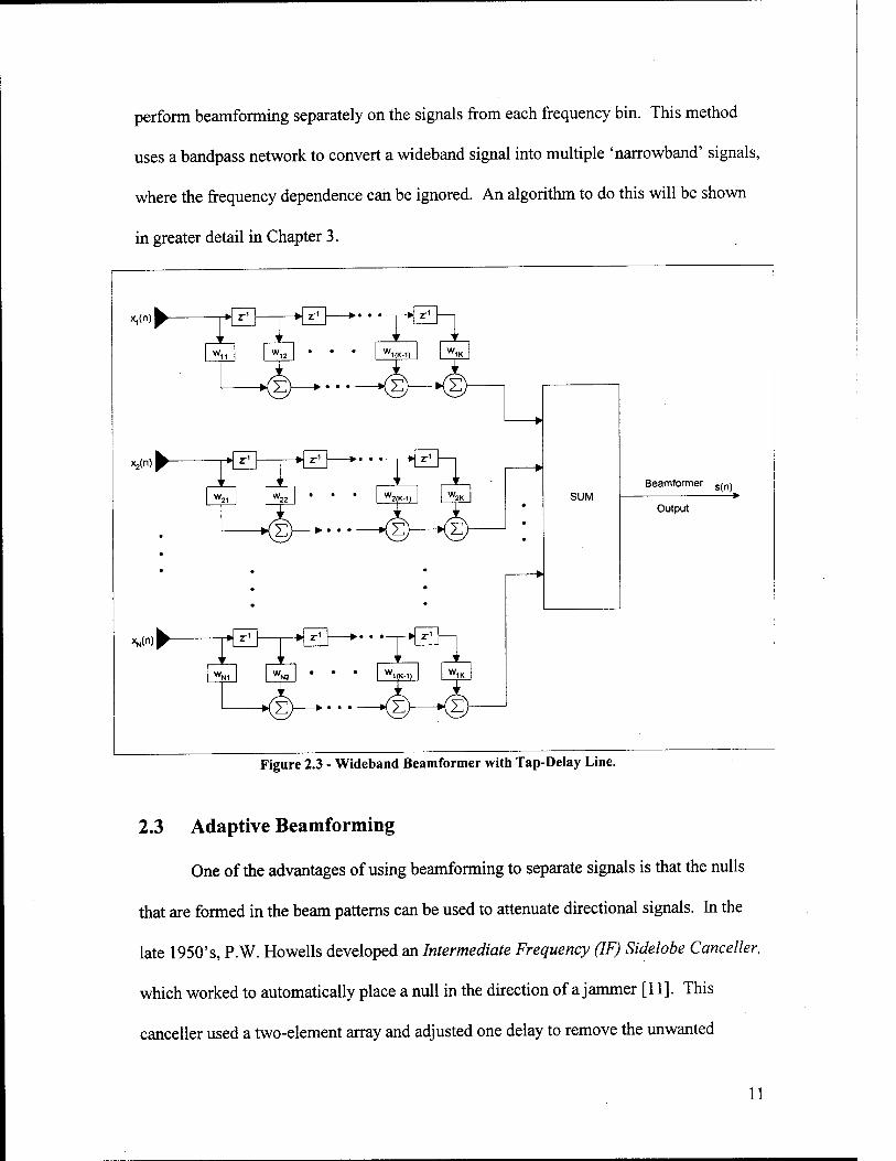
perform beamforming separately on the signals from each frequency bin. This method

uses a bandpass network to convert a wideband signal into multiple 'narrowband' signals,

where the frequency dependence can be ignored. An algorithm to do this will be shown

in greater detail in Chapter 3.

x,(n)^~

x>(n)

XNM

* z-1 > z-' ► > r'

£}—► £—K2

> z:1

"2(K-1)

-KS)—► ;s)—►(£)

* r1 ► z-1 * ' ' ' '

W1(K-1) W1K

E^- S)—KS

SUM Beamformer s(n)

Output

Figure 2.3 - Wideband Beamformer with Tap-Delay Line.

2.3 Adaptive Beamforming

One of the advantages of using beamforming to separate signals is that the nulls

that are formed in the beam patterns can be used to attenuate directional signals. In the

late 1950's, P.W. Howells developed an Intermediate Frequency (IF) Sidelobe Canceller,

which worked to automatically place a null in the direction of a jammer [11]. This

canceller used a two-element array and adjusted one delay to remove the unwanted

11

signal. In 1967, the first Least Mean Square (LMS) algorithm was developed for

adaptive arrays, which eventually become known as the optimum Wiener solution for

stationary inputs [11]. Other algorithms have been developed to improve the adaptive

beamforming problem including the use of constraints. The following sections will

present the basic LMS algorithm as presented by B. Widrow in 1967 [12]. Additionally,

constraints will be discussed in order for the reader to get a full picture of adaptive

beamforming.

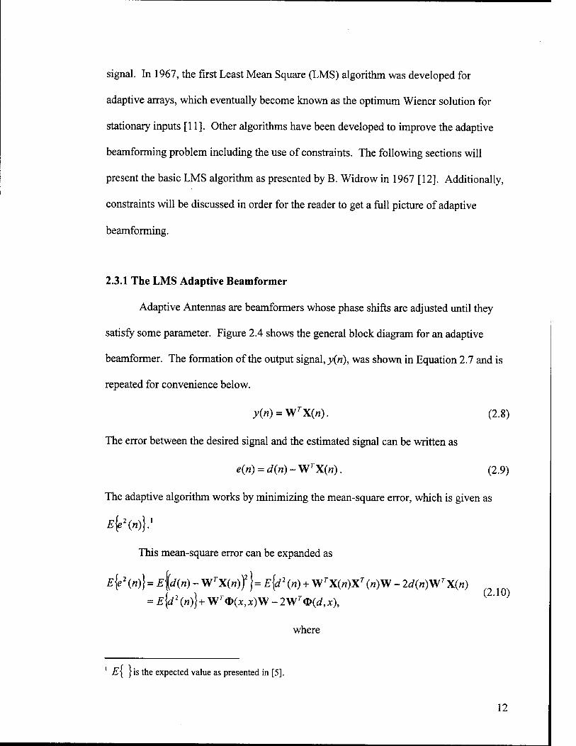
2.3.1 The LMS Adaptive Beamformer

Adaptive Antennas are beamformers whose phase shifts are adjusted until they

satisfy some parameter. Figure 2.4 shows the general block diagram for an adaptive

beamformer. The formation of the output signal, y(n), was shown in Equation 2.7 and is

repeated for convenience below.

y(n) = WrX(n). (2.8)

The error between the desired signal and the estimated signal can be written as

e{n) = d(n)-WTX(n). (2.9)

The adaptive algorithm works by minimizing the mean-square error, which is given as

E^{n)}}

This mean-square error can be expanded as

E{e2 (»)} = E\d(ri) - WTX(n))2}= E{d2 (n) + Wr X(«)Xr («)W - 2d(n)VfTX(n)

E{d2 («)}+ WrO(x, x) W - 2WT<J>(d,x),

where

(2.10)

E[ } is the expected value as presented in [5].

12

<D(x(n),x(n)) = E{x(n)XT (n)}=E

'^OO^O) xx{n)x2{n) •■■ xx{n)xN(n)

x2{ri)xx{ri) x2(n)x2(n) ••• x2(n)xN(n)

xN(n)xx(n) xN(n)x2(n) ••• xN(n)xN(n)

and

®(d(n),x(n)) = E{d(n)X(n)} = E-

d(n)xl (n)

d{n)x2(n)

d{n)xN(n)

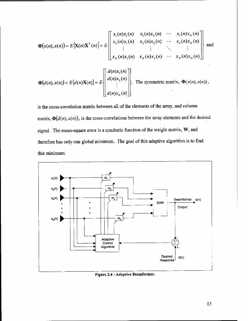
The symmetric matrix, <f>(x(ri),x(n))

is the cross-correlation matrix between all of the elements of the array, and column

matrix,<b(d(n),x{ri)), is the cross-correlations between the array elements and the desired

signal. The mean-square error is a quadratic function of the weight matrix, W, and

therefore has only one global minimum. The goal of this adaptive algorithm is to find

this minimum.

x,(n) ^~

Xj(n) ^~

X3<n) ^~

*.(") ►"

SUM Beamformer s(n) ►

Adaptive Control

Algorithm

Output

Desired Response

d(n)

Figure 2.4 - Adaptive Beamformer.

13

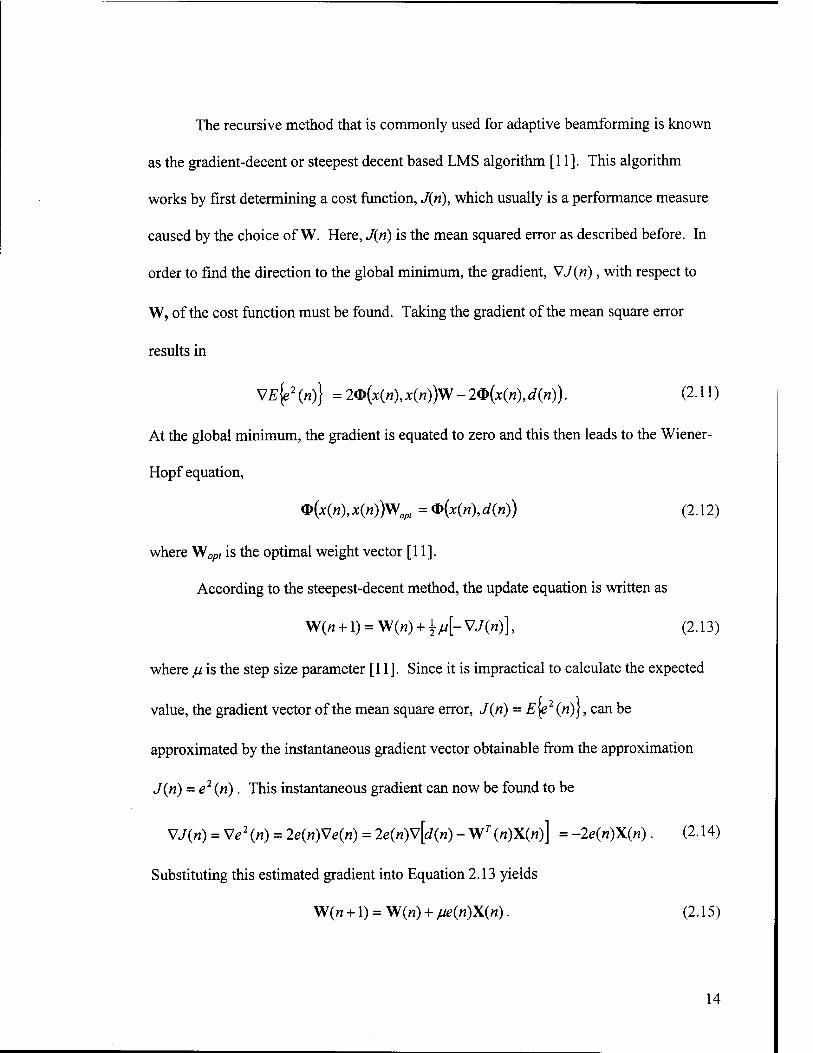
The recursive method that is commonly used for adaptive beamforming is known

as the gradient-decent or steepest decent based LMS algorithm [11]. This algorithm

works by first determining a cost function, J(n), which usually is a performance measure

caused by the choice of W. Here, J(n) is the mean squared error as described before. In

order to find the direction to the global minimum, the gradient, VJ(n), with respect to

W, of the cost function must be found. Taking the gradient of the mean square error

results in

V£{e2(«)} = 2*(JC(/I),X(/I))W-20(JC(H), </(«))• (2-11)

At the global minimum, the gradient is equated to zero and this then leads to the Wiener-

Hopf equation,

<p{x(n),x(n))\Vopt = fl>(*(«), d{nj) (2.12)

where W0/), is the optimal weight vector [11].

According to the steepest-decent method, the update equation is written as

W(« + l) = W(«) + ^[-VJ(«)], (2.13)

where ju is the step size parameter [11]. Since it is impractical to calculate the expected

value, the gradient vector of the mean square error, J(ri) = £{e2 («)}, can be

approximated by the instantaneous gradient vector obtainable from the approximation

J(n) = e2 (n). This instantaneous gradient can now be found to be

VJ(») = Ve2(n) = 2e(n)Ve{n) = 2e{n)v[d(n) - Wr(w)X(/i)] = -2e{n)X(n). (2.14)

Substituting this estimated gradient into Equation 2.13 yields

W(« + l) = W(w) + //e(«)X(w). (2.15)

14

This estimate of the gradient is now considered noisy, however, as n -> as, the expected

value of W converges to Wopl if 0 < ju < —, where Amax is the largest eigenvalue from max

the matrix <b{x(n),x(n)) [11].

The algorithm in Equation 2.15 minimizes the noise added to the desired signal by

placing nulls in the directions of the noise sources. This algorithm requires that the

desired signal be known in order to minimize the mean-square error. Having a reference

signal that is correlated to the desired signal can also be used which lessens this

restriction [13]. In order to obtain a correlated reference signal, a priori information

about the signal must be known. In this thesis, it is assumed that no a priori information

about the sources is known, which rules out these types of algorithm to separate passive

sources.

Another advantage to the IC A blind beamformer is that traditional adaptive

beamforming is based on second order statistics (mean square error, maximization of

SNR, minimization of variance), where the ICA blind beamformer uses implicitly all

higher moments. This provides better separation of non-Gaussian signals.

2.3.1 Constraints

The LMS algorithm places nulls in the direction of the noise sources, but has no

control on where the main beam gets positioned. In 1972, O.L. Frost developed a

constrained LMS algorithm in order to keep the main beam focused in the direction of the

desired source [8]. Assuming the direction of the source is known, this is done by

keeping

15

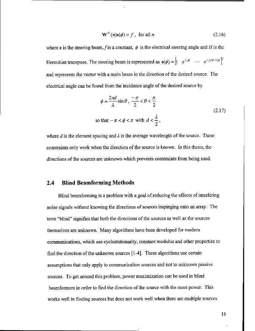
W"(/i)s(0) = /, for all« (2.16)

where s is the steering beam,/is a constant, <p is the electrical steering angle and H is the

Hermitian transpose. The steering beam is represented as s(^) = [l e'1* ■■■ e'J(M~^\

and represents the vector with a main beam in the direction of the desired source. The

electrical angle can be found from the incidence angle of the desired source by

, 2nd . -7t n 6 = sin#, <9 < — Y X 2 2

so that -7t <6<n with d < — , Y 2

(2.17)

where d is the element spacing and X is the average wavelength of the source. These

constraints only work when the direction of the source is known. In this thesis, the

directions of the sources are unknown which prevents constraints from being used.

2.4 Blind Beamforming Methods

Blind beamforming is a problem with a goal of reducing the effects of interfering

noise signals without knowing the directions of sources impinging onto an array. The

term "blind" signifies that both the directions of the sources as well as the sources

themselves are unknown. Many algorithms have been developed for modern

communications, which use cyclostationarity, constant modulus and other properties to

find the direction of the unknown sources [1-4]. These algorithms use certain

assumptions that only apply to communication sources and not to unknown passive

sources. To get around this problem, power maximization can be used in blind

beamformers in order to find the direction of the source with the most power. This

works well in finding sources but does not work well when there are multiple sources

16

with similar power. The following sections will present some of these blind

beamforming methods.

2.4.1 Cyclostationarity

One of the first blind beamforming algorithms was developed to take advantage

of cyclostationarity. Cyclostationarity applies to signals that have periodic statistical

averages [5]. For wide sense cyclostationarity, the mean and variance can be time

varying and periodic [5]. Many digital modulated signals are considered cyclostationary

and have either a cycle frequency (frequency of time-varying statistics) double to the

carrier frequency, a multiple of the baud rate or both [1]. This blind beamforming

algorithm takes advantage of this properly because most interfering noise signals do not

have these cyclostationarity properties. This algorithm requires that the signal of interest

or interfering signal have cyclostationarity properties. For passive sources, there is no

guarantee that the signals will have cyclostationarity properties. It is therefore not a

practical method to separate passive sources.

2.4.2 Constant Modulus

Most digitally modulated signals including FSK, PSK and 4-QAM have constant

envelopes. A constant modulus blind beamformer works by updating the taps in order to

make the output have a constant envelope. As with the cyclostationarity property, most

noise and interfering signals do not have constant envelopes. This algorithm works well

when finding one digitally modulated signal in noise. It can be used to find more than

one digitally modulated signals if the signals are statistically independent. Multiple

17

signals are removed in stages where the first stage removes one signal from the mixture.

The extracted signal is then removed from the mixture for further processing. The next

stage repeats until all of the signals are removed [1]. This algorithm has a slow

convergence rate and works mostly for digitally modulated signals. This algorithm

would not work on passive sources since it cannot be assumed that the sources have a

constant modulus.

2.4.3 The JADE Algorithm

In 1993, J.F. Cardosa and A. Souloumiac developed an 'off-line' beamforming

technique known as joint approximate diagonalization of eigenmatrices (JADE) [14].

This algorithm is a two-step process, which separates multiple directional signals by

exploiting the statistical independence of the sources. The first step exploits second order

moments by "whitening" the array output vector, which results in the sources mixed by

an unknown unitary matrix. The second step consists of estimating this unknown unitary

matrix by "joint diagonalization" of the forth order cumulant matrices of the "whitened"

data [21]. This algorithm has also been improved by J. Sheinvald in 1998 and M. Wax

and Y. Anu in 1999 by finding the unitary matrix using a least squares approach [15,16].

JADE is considered a batch-processing algorithm because it requires the entire

data set for processing. This limits this algorithm to 'off-line' applications. This

algorithm also results in a permutation of the outputs. This permutation limits the direct

knowledge of the direction of the separated signal. This algorithm also separates signals

based on second and fourth order moments. The ICA blind beamformer that will be

presented in this thesis will use all even order moments to blindly separate the sources,

18

which provides a better estimate of independence. The directions of the sources will also

be estimated directly in the ICA blind beamformer.

2.4.4 Power Maximization Techniques

There are many blind beamforming methods that find the direction of the signal

with the most power. The learning rule for maximizing power with the norm constraint

for the adjustable weights is given as

maxwffRw subject to w^w = 1, (2.18)

where w is the weight matrix and R = E\x(n)xH («)} is the autocovariance matrix of the

data inputs. Recently, blind beamforming algorithms have been developed in order to

satisfy Equation 2.18 for code division multiple access (CDMA) mobile communications

[2]. Instead of using an adaptive algorithm to learn the ideal weights, the algorithm finds

the eigenvector corresponding to the largest eigenvalue of the autocovariance matrix, R.

The weight vector is then set to the corresponding eigenvector, which places the main

beam in the direction of the source with the most power. Preprocessing is done on the

mixtures of comparable power CDMA signals, which attenuates the undesired signals.

The resulting power maximum is then the likely direction of the desired source. This

algorithm works well for mixtures when the desired signal has the most power, but does

not work as well when the signals have similar power. This algorithm does nothing

beyond focusing the main beam on the desired signal in order to minimize the noise level

from the interfering signals. It does not use the positioning of the nulls in the beam

pattern to remove the interfering signals.

19

In 1996, Chit-Sang Tsang and R. T. Compton developed an adaptive blind

beamformer that works on power maximization [17]. They presented an algorithm that

can be used to separate a strong interfering signal from a weak signal using a two-

element array. This algorithm uses time delay beamforming to steer the main beam or a

null in the direction of the signal with the most power. This algorithm is the basis of the

ICA blind beamformer and will be improved by using statistical independence as a

criterion.

The following derivation will assume an antenna array with N element and a

uniform element spacing of L. For narrowband signals, the element spacing is commonly

set to half the wavelength of the carrier frequency. For wideband signals, the element

spacing is usually set to half the wavelength corresponding to the center frequency or the

largest frequency. The output of the antenna elements are connected to time delays and

then summed. The algorithm works by adjusting the time delays, which changes the look

direction.

The signals from the individual elements can be represented in matrix form as

x = [*!(t) x2(t) •■■ xN(t)\ . The signals from the elements are then individual

delayed and can be rewritten as y = [x, (t - dx) x2(t-d2) ■■■ xN(t - dN)f =

\)>\ (0 ^2 (0 "" yN (0 jr • The output signal from the beamformer is

s(t) = y,(t) + y2(t) + ... + yh/(t) = x](t-dl) + x2(t-d2) + ... + xN(t-dN). (2.19)

The times delays d\t di,... , d^ adapt in order to maximize the power of the output. The

power of the output (also the cost function) for real signals can be written as

J(t) = E\s2(t)} . (2.20)

20

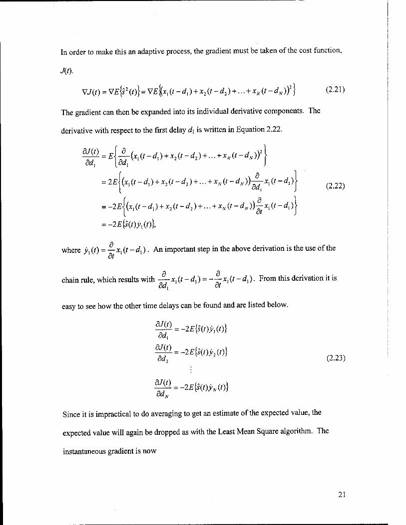
In order to make this an adaptive process, the gradient must be taken of the cost function,

J{t).

VJ(t) = VE{s\t)} = VE\xx(t-dx) + x1(t-d1) + ... + xN(t-dNjf} (2.21)

The gradient can then be expanded into its individual derivative components. The

derivative with respect to the first delay d\ is written in Equation 2.22.

dJ{t) ddx

= E\^-{xl(t-dl) + x2(t-d2) + ... + xN(t-dN))2\

= 2EUxx(t-dx) + x2(t-d2) + ... + xN(t-dN))—xx(t-dx)\

= -2EUxx(t -dx) + x2(t -d2) +... + xN(t -dN))-xx(t-dx)i

(2.22)

= -2E{s(t)yM

where yx (t) = —xx(t-dx). An important step in the above derivation is the use of the dt

chain rule, which results with xx (t - dx) = -—xx (t - dx). From this derivation it is ddx dt

easy to see how the other time delays can be found and are listed below.

d-^l = -2E{sm(0] odx

yg—imM-)] _,,. dd2 (2.2J)

^l = -2E{s(t)yM ddN

Since it is impractical to do averaging to get an estimate of the expected value, the

expected value will again be dropped as with the Least Mean Square algorithm. The

instantaneous gradient is now

21

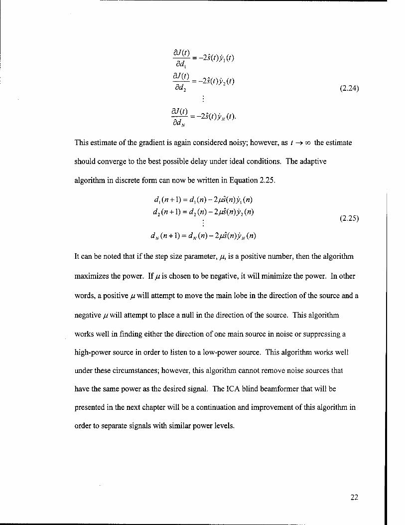
odx

dd2 (2.24)

ddN

This estimate of the gradient is again considered noisy; however, as t -» oo the estimate

should converge to the best possible delay under ideal conditions. The adaptive

algorithm in discrete form can now be written in Equation 2.25.

dx (n +1) = dx (n) - 2jus(n)yx (n)

d2(n + \) = d2(n)-2jus(n)y2(n)

dN (n + l) = dN («) - 2fJs(n)yN (n)

It can be noted that if the step size parameter, ju, is a positive number, then the algorithm

maximizes the power. If/i is chosen to be negative, it will minimize the power. In other

words, a positive JJ. will attempt to move the main lobe in the direction of the source and a

negative fj. will attempt to place a null in the direction of the source. This algorithm

works well in finding either the direction of one main source in noise or suppressing a

high-power source in order to listen to a low-power source. This algorithm works well

under these circumstances; however, this algorithm cannot remove noise sources that

have the same power as the desired signal. The ICA blind beamformer that will be

presented in the next chapter will be a continuation and improvement of this algorithm in

order to separate signals with similar power levels.

22

2.5 Other Methods

2.5.1 Blind Source Separation

In 1986, Jeanny Herault and Christian Jutten developed an algorithm based on

Neural Networks that they claimed could blindly separate mixtures of independent

signals [18]. This new algorithm began a new era in signal processing known as blind

source separation (BSS). There algorithm worked by setting a non-linear cross-

correlation function to zero, instead of the linear cross-correlation. The learning rule for

this algorithm is

AWy oc f(u,)g(uj)T fori*j, (2.26)

where/and g are odd non-linear functions and ut is the zth output. The diagonals in W

are set to zero in this algorithm. The output vector is found for every iteration by

u(«) = (l + W)-1x(«), (2-27)

where x(«) = [*,(") *2(«) *s00 - ^ («)F is the input vector, and I is an identity

matrix. These non-linear functions are important to this algorithm because linear

techniques only exploit second-order moments, which do not truly separate signals that

have non-Gaussian distribution functions. Non-linear techniques take advantage of these

higher order cross-moments and in turn help create true statistical independence. This

algorithm was shown to only work on specific types of sources; however, it opened the

door to a whole new set of algorithms.

In 1995, Anthony J. Bell and Terrence J. Sejnowski developed an algorithm that

separated mixed sources based on Information Theory, which became the basis for

modern BSS methods [19]. Their algorithm learned the unmixing matrix by maximizing

23

the mutual information between the inputs and the outputs. Their learning rule which

used the non-linear function, tanh, is

AW oc [wr ]"' - 2 tanh(\Vx)xr, (2.28)

where x = [x, x2 x3 ... xN]T is the input vector and W is the learned unmixing

matrix. This algorithm worked well in separating sources that had both super-Gaussian

(negative kurtosis) and sub-Gaussian (positive kurtosis) distribution functions.

In 1997, S. Amari, S.C. Douglas, A Cichocki, and H.H. Yang improved Bell and

Sejnowski's algorithm. Their new algorithm used a natural gradient approach to

minimize the Kullback-Leibler distance between the individual output PDFs and product

of the output PDFs [20]. The Kullback-Leibler distance is a measure of dependency

between the output distributions [21]. Their learning rule is

AWocIl-ytuV] W, (2.29)

where u = [w( u2 w3 ... uN\ is the output vector. This new algorithm sped up the

processing time by removing the need for a matrix inversion as presented in the Bell and

Sejnowski's algorithm.

All of these information theoretic BSS algorithms, known as infomax algorithms,

work by learning an unmixing matrix, W, which satisfies WA = PD where A is the full

rank mixing matrix, P is a permutation matrix and D is a diagonal matrix. The

permutation matrix, P, prevents a direct estimate of what sensor or what direction the

signal came from. A block diagram of a general BSS algorithm is shown in Figure 2.5.

It should be noted that before the data is sent through the BSS algorithm, the mean is set

2 The non-linear function tanh() is commonly used in BSS because it works well in separating sources with multiple types of probability distributions.

24

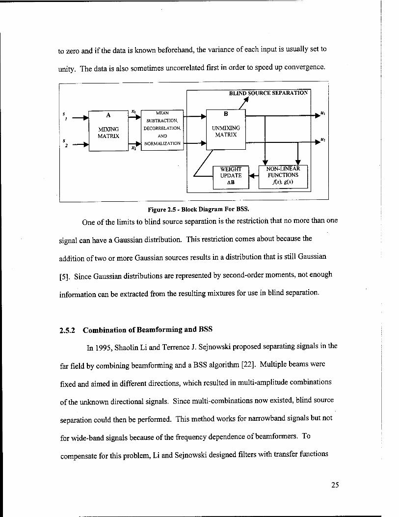
to zero and if the data is known beforehand, the variance of each input is usually set to

unity. The data is also sometimes uncorrelated first in order to speed up convergence.

MIXING MATRIX

X\

Xl

MEAN

SUBTRACTION,

DECORRELATION,

AND

NORMALIZATION

BLIND SOURCE SEPARATION

B

UNMIXING MATRIX

WEIGHT UPDATE

AB

NON-LINEAR FUNCTIONS

.«i

.«2

Figure 2.5 - Block Diagram For BSS.

One of the limits to blind source separation is the restriction that no more than one

signal can have a Gaussian distribution. This restriction comes about because the

addition of two or more Gaussian sources results in a distribution that is still Gaussian

[5]. Since Gaussian distributions are represented by second-order moments, not enough

information can be extracted from the resulting mixtures for use in blind separation.

2.5.2 Combination of Beamforming and BSS

In 1995, Shaolin Li and Terrence J. Sejnowski proposed separating signals in the

far field by combining beamforming and a BSS algorithm [22]. Multiple beams were

fixed and aimed in different directions, which resulted in multi-amplitude combinations

of the unknown directional signals. Since multi-combinations now existed, blind source

separation could then be performed. This method works for narrowband signals but not

for wide-band signals because of the frequency dependence of beamformers. To

compensate for this problem, Li and Sejnowski designed filters with transfer functions

25

that were designed to undo the filtering effects of the beamformers. The source

separation method used in the paper was the Herault-Jutten method. The probable reason

for this selection was that the infomax algorithms were not developed yet. The Herault-

Jutten algorithm could then be replaced with an infomax algorithm for better results. The

main drawback to this algorithm is the permutations that are caused from the source

separation algorithms. The permutations prevent the algorithm from directly estimating

the directions of the incoming signals.

26

Chapter 3. ICA Blind Beamforming

3.1 Overview

The techniques that were described in the previous chapter were all techniques that

are currently used to separate signals blindly. Depending on the applications, some of

the techniques worked better than others. For passive sources with unknown locations,

none of these algorithms gave adequate source separation while simultaneously finding

the directions of the sources. In this chapter an algorithm will be presented to do source

separation and direction finding simultaneously by applying an independence criterion to

blind beamformers. It will be assumed in this thesis that the number of sources is known.

Performing blind separation techniques without the knowledge of the number of sources

is still an outstanding research problem [16, 23, 24].

3.2 ICA Blind Beamformer

3.2.1 Independence Technique

The independence-based blind beamformer presented here is similar to the power

maximization techniques as presented in Chapter 2.4.4; however, it works for more than

one directional signal. The goal of the independence technique is to minimize either the

correlation or non-linear correlation between the two outputs of the algorithm. For

example, if there are two signals from different directions arriving at the array, then the

algorithm will place a beam in the direction of one source and a null in the direction of

other interfering source. It will also do the opposite by placing a beam on the interfering

27

source and a null in the direction of the desired source. This method will find the

direction of both sources and provide an estimate of the both signals.

As with the power maximization beamformer, this algorithm will use the gradient

descent search method. All derivations will be made for real signals. In the first case

that will be presented, the algorithm will use a linear process, which minimizes the cross-

correlation between the two outputs. The absolute value of the cross correlation between

the outputs of two beamformers can be written as

J(0 = 1^,(0*2(0)1, (3-D

where i, (0 is the output of beam one and s2 (t) is the output of beam two. The absolute

value is there because it is possible for the cross-correlation to become negative. If a

source is located in one of the odd numbered sidelobes, the source will be received by the

beamformer with a sign change. Because of this sign change, a negative cross-

correlation will result. The absolute value will make the true minimum of the cost

function in Equation 3.1 equal to zero. By compensating for this sign shift, the nulls

from the beam pattern should be steered in the direction of the opposing sources and

result in better statistical independence.

In this section, the reference point for the array will be the center element of an

odd element array (this algorithm can be easily expanded for a even-element array but

will be left out for brevity). Keeping the reference point at the center of the array will

eliminate additional delay terms at the array. If the reference point is not at the center,

then an additional delay can result. These delays can be a problem for the cost function

in Equation 3.1, if these delays become larger than the correlation time, x0, of the signals,

where the correlation time is defined as the smallest delay that satisfies

28

E{x(t)x(t - T0)} = 0. If this occurs, then the signals will appear to be uncorrelated, which

will result in a false convergence. The only disadvantage to using beamformers with a

central reference point is that the process becomes non-causal, which can be compensated

for by adding a buffer. The amount of the delay the buffer adds; however, is very small

compared to the length of signals. The beam is then formed as

hM = xllf + ^dk)+...xe(t) + ...xN((-ypdk) (32)

where xc (/) is the center element. As before, the gradient must be taken of the cost

function, J{f), in order to make it an adaptive process.

VJ(0 = V\E{sx (t)s2 (0 J = sgn[£[s, (t)s2 (0}]V£fe (t)s2 (f)}

= sgn[£{lI(fÄ(O}]-v4xI(f-^rf0+... + xe(0+... + x^(r + ^i/1))* (3.3)

(Xl(t-^d2)+... + xAt)+... + xN{t + ^d2))}

There are now two sets of delays for the separation of two signals, one for the estimate of

each signal. The gradient of the first delay d\ is written below.

^ = sgn[£{i, (t)s2 (/)}] • E^- 5, (f)s2 (0J

= sgn[£{j,(0i2(0}]-

=sgn[^^o^(o}]^k(o^-(x1(/+«^)+...+^(^-i¥1^))l

(3.4)

ddx

8 = sgn [£fc(/)i2(0}]-£52(0|(x1(r + ^^)+...-x,(f-^rfI))

dt

= sgn[^1(Oi2(O}]-4a(O(1¥I>'n(0+----1¥1^(4

where > A (0 = — x (t-dk). The estimate of the second signal can also be easily p dt p

proved and is listed below.

29

^ = sgn[E{s,(t)sM]-E{sM^y2Ath...-^y2M} (3.5) oa2

The expectation is again dropped for the same reasons as described in Chapter 2. The

expectation is also removed from the sign operator. Chapter 3.2.4 will propose a method

to determine sgn^ji, {t)s2 (0}]> which will provide better results. The adaptive

algorithm in discrete form is shown in Equation 3.6.

^(« + l) = c/1(»)-//-sgn[51(^(«)]^2(n)(^>^«)+...-^j>1/VW)

J2(« + l) = ^(«)-//-sgn[i1(«)i2(«)]J1(»)(^>21(«) + ...-^^W)

It should also be noted that the step size parameter, fj., should be a positive number in

order to minimize the cross-correlation. A negative ju will maximize the cross-

correlation; hence it will position the two beams in the same direction. This algorithm

can be easily expanded for more than two signals. The discrete algorithm for this is listed

below with M representing the number of sources and/? representing the beam number.

^(« + l) = Jp(«)-//-(^^1W + ...-^j>pj4isgn^(^(«)]-^(") (3-7)

This algorithm minimizes the cross-correlation between the beam of interest and all the

other beams.

The above derivations were for an algorithm that minimizes the cross-correlation

between the beams. Minimizing the cross-correlation will only minimize the second

cross-moment while the other higher order moments can still be non-zero. For true

statistical independence, all higher order cross-moments should be zero. One way to set

all of the higher order moments to zero is to use a odd non-linear function, J[-), in the

algorithm as with Independent Component Analysis (ICA). If the cost function, J{f), is

30

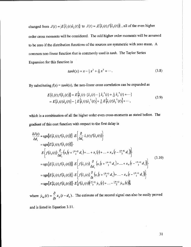
changed from J{t) = \E{sx{t)s2{t)\ to J(t) = \E{sx(t)f(s2(t))] , all of the even higher

order cross moments will be considered. The odd higher order moments will be assumed

to be zero if the distribution functions of the sources are symmetric with zero mean. A

common non-linear function that is commonly used is tank. The Taylor Series

Expansion for this function is

tanh(x) = x-\x3+±x5+---. (3.8)

By substituting/*) = tanh(x), the non-linear cross correlation can be expanded as

£fe(0/fe(0)} = £&(')■ ih (t)-\s2\t)+±s2\t) + -]

= E{s{ (t)s2 (0} - \ E^ (t)s23 (0}+ £ 4i (0 V (0}+

(3-9)

which is a combination of all the higher order even cross-moments as stated before. The

gradient of this cost function with respect to the first delay is

(3.10)

^f = sgnfeft (/)/& (0)}] • E^ i, (0/fc (0)|

= sgn[£{s1(0/(52(0)}]-

= sgnfeft(/)/&«)}]• *{/& (0)^ (*, (' + (T? 4)+ ■ • • + x, (/ - ^ 4))

= sgn[£{Sl(/)/(S2(0)}]^^

=sgD[£{sI(/)/(*2(o)}]-^(oX^Ä.(0+...-ö^^(0j

where yk(t) = —x (t-dk). The estimate of the second signal can also be easily proved p dt p

and is listed in Equation 3.11.

31

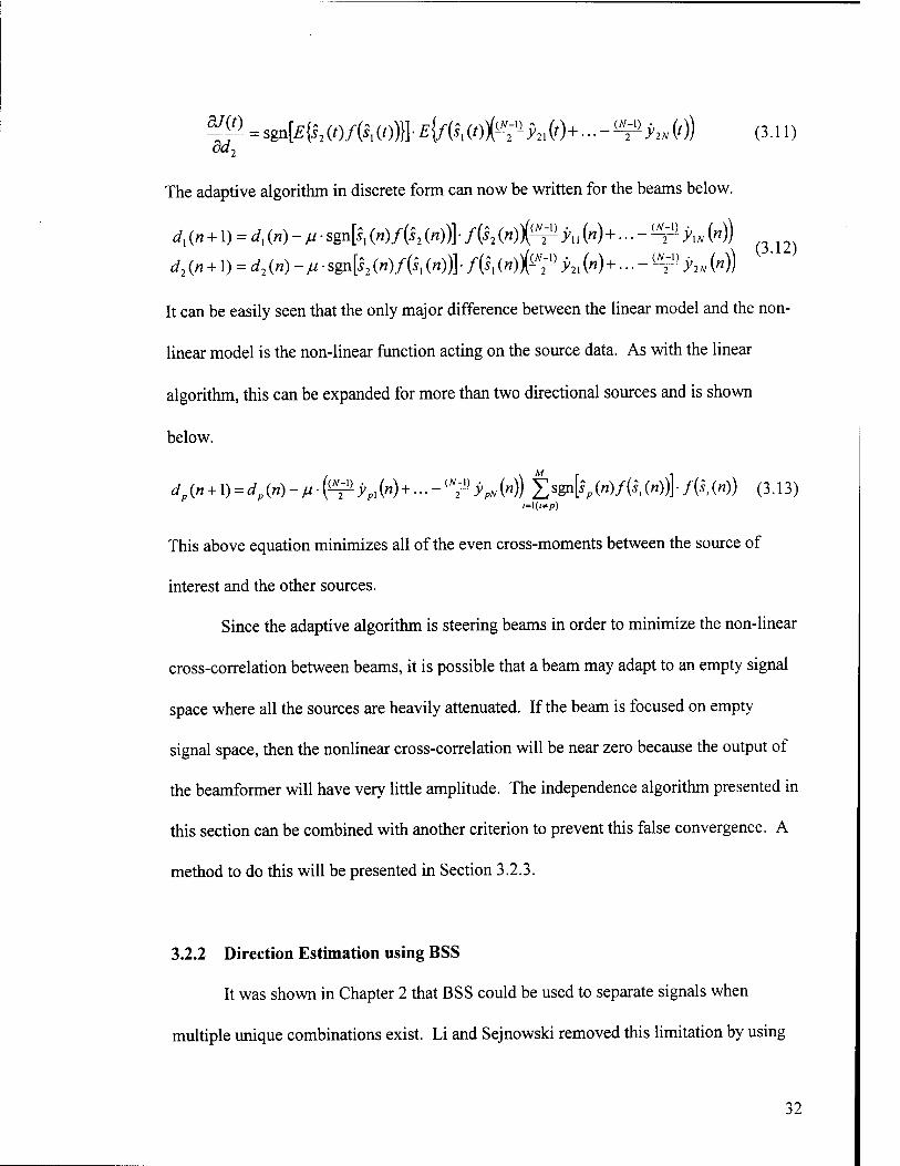
^»sgn^CO/ftCOja-^feCO^^W+.-.-^^W) (3.11)

(3.12)

The adaptive algorithm in discrete form can now be written for the beams below.

d2 (n +1) = d2 (n)-ju- sgn[s2 (»)/& (»))] • /(s, («))(^ j>21 («)+... - ^ y2N ("))

It can be easily seen that the only major difference between the linear model and the non-

linear model is the non-linear function acting on the source data. As with the linear

algorithm, this can be expanded for more than two directional sources and is shown

below.

dp(n + \) = dp(n)-Mi^yM+----^KMiMh(n)Äs^)lf("^) (3-13)

This above equation minimizes all of the even cross-moments between the source of

interest and the other sources.

Since the adaptive algorithm is steering beams in order to minimize the non-linear

cross-correlation between beams, it is possible that a beam may adapt to an empty signal

space where all the sources are heavily attenuated. If the beam is focused on empty

signal space, then the nonlinear cross-correlation will be near zero because the output of

the beamformer will have very little amplitude. The independence algorithm presented in

this section can be combined with another criterion to prevent this false convergence. A

method to do this will be presented in Section 3.2.3.

3.2.2 Direction Estimation using BSS

It was shown in Chapter 2 that BSS could be used to separate signals when

multiple unique combinations exist. Li and Sejnowski removed this limitation by using

32

beamforming in order to create unique combinations [22]. For narrowband signals, the

only effect that beamformers have is amplitude adjustments, which is dependent on the

direction of the signals. Therefore, the output of the multiple beamformers can be written

as V = AS, where V = [v, v2 ... vN f is the output, S = [s, s2 ... sN J is the

original signal matrix and A is an unknown NxN mixing matrix resulting from the

beamformers. If the signals are wideband, then the filtering effects of the beamformer

have to be incorporated in the algorithm, which generalizes the elements of the mixing

matrix, A, to filters from constants. The mixing matrix will also have to incorporate time

delays if the mixtures of signals are mixed and arbitrarily delayed. Algorithms have been

written for both of these applications in many papers in order to find these unknown

delays and unknown filters [25-27]. Since beamformers with central reference points are

being used to create these combinations for narrowband signals, no delays will be

created.

In order for BSS to work, there has to be at least as many mixtures of signals as

there are signals. Therefore, there must be at least N beams that are focused in different

directions. Assuming that each signal has its own direction, there will be N unique

mixtures. Since N mixtures are now initially formed, BSS can be used to separate these

mixtures and return an estimate of the original N separated signals. For example, the

outputs from the two individual beams, vl (f) and v2 (0, are used as inputs to the BSS

algorithm which result in discrete outputs «, (n) and u2 («). Any BSS algorithm can be

used for this application. For purposes of this paper, Armari's Natural Gradient

Algorithm [20] will be used, which was described in Chapter 2 and is repeated below for

convenience.

33

AWoc[l-/(uy] W, (3-14)

This BSS algorithm learns an unmixing matrix, W, and uses it to separate the signals. It

is again possible for the outputs to be permuted. This permutation is what limits the

algorithm from directly estimating the directions of propagation.

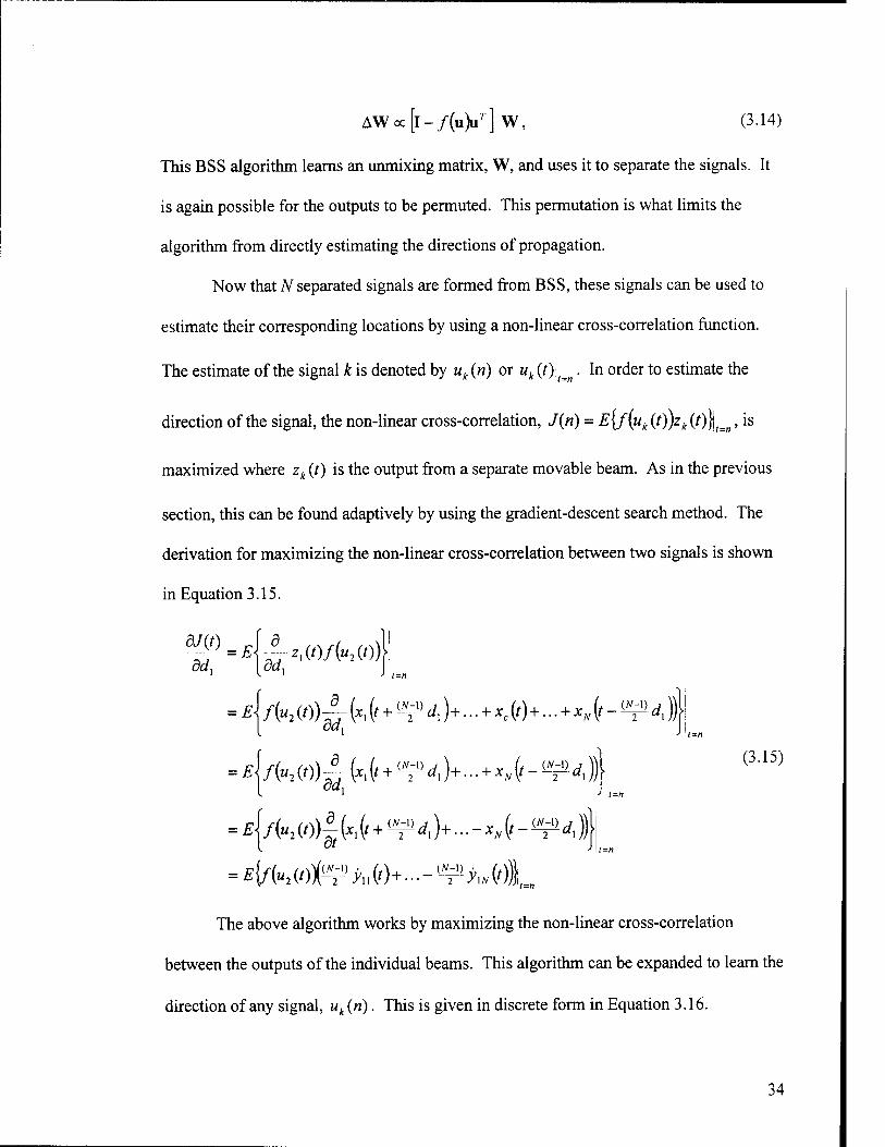
Now that N separated signals are formed from BSS, these signals can be used to

estimate their corresponding locations by using a non-linear cross-correlation function.

The estimate of the signal k is denoted by uk (n) or uk (t)\i=n. In order to estimate the

direction of the signal, the non-linear cross-correlation, J(n) = E{f(uk (t))zk (t)\l=n, is

maximized where zk (t) is the output from a separate movable beam. As in the previous

section, this can be found adaptively by using the gradient-descent search method. The

derivation for maximizing the non-linear cross-correlation between two signals is shown

in Equation 3.15.

dJ{t)

ddx = £J~S,(0/(«2 ('))}'

4/(«2 ('))£(*, (> + ^ dx)+... + x, (/ - ^ 4 ))l (3.15)

= £{/(ii2(0)|(x1(f + ^rf1)+...-xJ,(r-^^))|

The above algorithm works by maximizing the non-linear cross-correlation

between the outputs of the individual beams. This algorithm can be expanded to learn the

direction of any signal, uk (n). This is given in discrete form in Equation 3.16.

34

dk(n + l) = dk(n) + ß-f(ukwi^hM+----^hM) (3-16)

It again should be noted that the step size parameter, ß, should be positive in order to

maximize the non-linear cross-correlation.

This algorithm works by using stationary beams to create multi-amplitude

mixtures for which BSS is used to separate the signals. A separate movable beam is then

adjusted in order to maximize the non-linear cross-correlation between the beam and the

outputs of the BSS algorithm. The resulting beam patterns will have the main beams

focused in the direction of the multiple sources.

3.2.3 Combination of Independence and Direction Estimation Techniques

Chapter 3.2.2 reintroduced Li and Sejnowki's algorithm, which uses stationary

beams and BSS to estimate the unmixed signals. It was then expanded to use separate

movable beams in order to estimate the directions of the respective signals. This

algorithm does not take advantage of some of the properties of beamformer such as the

placement of nulls. This section will combine this technique with the independence

technique as presented in Section 3.2.1 to use the same beams to separate the signals and

find their respective directions.

The algorithm in Section 3.2.2 completely relied on the BSS algorithm to separate

the signals. It would be advantageous to not only use BSS to separate the signals, but

also use the beamformers to place nulls in the directions of the opposing signals.

Combining the algorithms in Sections 3.2.1 and 3.2.2 will do this. If sk(t) is an output

from a beam and ut (t)\ is an estimated signal from the BSS algorithm then by

35

maximizing E{f(uk(t))sk(t)}\i=n and concurrently minimizing \E\f(uk(t))s (r)| , t=n

where k± j, should separate the sources. This will maximize the non-linear cross-

correlation between the beam outputs and the estimated signals. It will also minimize the

non-linear cross-correlation between the beams and the opposing estimated signals. The

adaptive algorithm for this is written in discrete form in Equation 3.17.

</, (/i +1) = dx (») + /?■ /(«, (njJF?- >„(»)+...- ^ ylN (»))

-i«-sgn[i1(/i)/(«2(/i))]./(ii2(n))(M^I(/i)+...-^^(»))

- M ■ sgn[s2 (n)f(ux (»))] • /(«, («))(^i) >21 („) + ..._ UJ!> J>2A/ („))

(3.17)

In the above algorithm, fj. and yö are both positive step size parameters. They can both be

equal or they can be different depending on the application. In this paper, /j will be set

smaller than ß in order to move the beam into the direction of the source with the

constraint that the outputs of the beams should be independent. As before, the algorithm

can be expanded for more than two signals and is in general form below.

dp(n + \) = dp(n) + ß-f(up(n)\^ypXn) + ...-^yJn))

-//■(^>p,W+...-^^W)Zs8n[Äp(n)/(ii/(/i))]-/(«<(^ (3.18)

i=\(i*p)

This algorithm separates these signals without using any a priori information about the

incoming signal waveforms and their location. A block diagram for this algorithm is

shown in Figure 3.1 for two beams using an TV-element array.

There are many advantages to the algorithm in Equation 3.18 compared to the

algorithm Equation 3.13. Since estimates of the original signals are found by utilizing

BSS, maximization of the cross-correlation between the beams and the unmixed sources

36

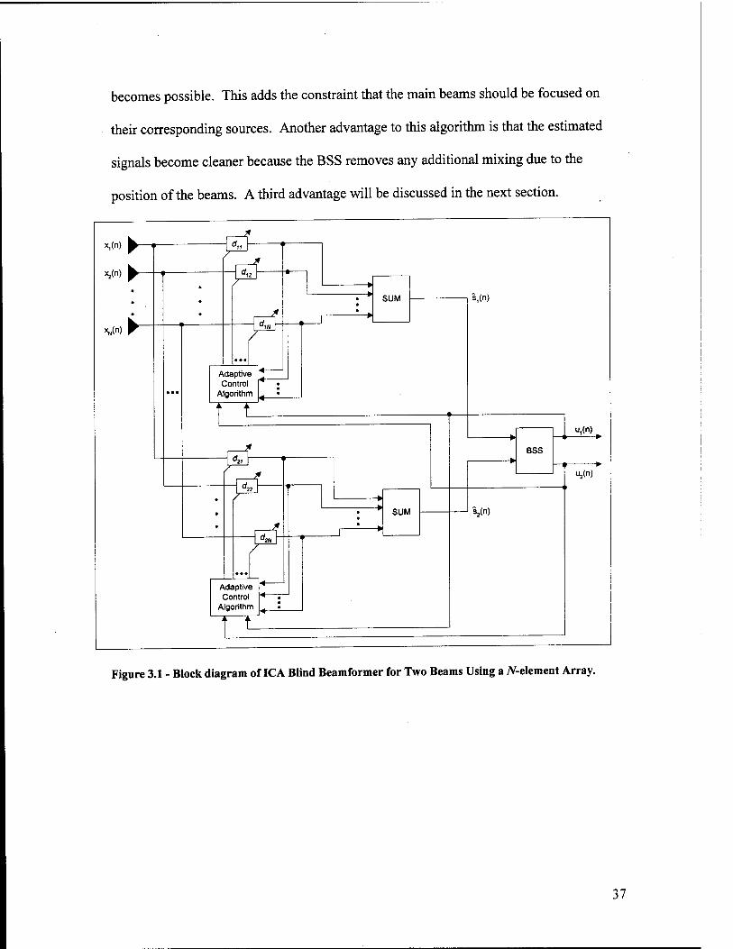
becomes possible. This adds the constraint that the main beams should be focused on

their corresponding sources. Another advantage to this algorithm is that the estimated

signals become cleaner because the BSS removes any additional mixing due to the

position of the beams. A third advantage will be discussed in the next section.

x,(n) ^~

Adaptive Control

Algorithm

•—r

Adaptive Control

Algorithm

SUM

SUM

s.(n)

BSS

u,(n)

s,(n)

Uj(n)

Figure 3.1 - Block diagram of ICA Blind Beamformer for Two Beams Using a W-element Array.

37

3.2.4 Step Size Parameter Control

The step size parameters are important part of the convergence process, which

were not discussed in much detail in the previous sections. In the last section, /j. and ß

were chosen to be constants; however, they do not need to be. Both ju and ß can be

adjusted during the process in order to optimize results. One way to do this is to increase

ju and ß when the delay estimates are far away from the optimum solutions and to

decrease them when they are close to the optimum solution. A measure of this can be

found by utilizing the unmixing matrix from the BSS algorithm. Another advantage to

using BSS for step size parameter control is that the sign of the unmixing matrix elements

can be used to determine sgn[£{5 (ri)f(u: («)))J , which can be used to replace

sgn[sp («)/(«, (n))\ in Equation 3.18.

The unmixing matrix is a good reflection on how independent the estimated

signals are from each other. If the signals are independent and the diagonals of the

unmixing matrix are kept to unity, then the non-diagonal elements should be near zero. If

the estimated signals still have combinations of each other, then the non-diagonals should

not be zero. This is because the unmixing matrix is estimating the inverse of the mixing

matrix. The adaptive algorithm can then be rewritten for this below.

dp(n + \) = dp(n) + ßp(n)-f{up(n)l^ypl(n)+...-^yJn))

-(^>)+--^vw) i>, (»)/(«>)) (3'19) i=\(i*p)

The step size parameter, ju{n), can be found by utilizing these non-diagonal elements and

can be written as

38

//„(/!) =-A/■*„(«), (3.20)

where fi is a constant and 5P,<«) is the element of the unmixing matrix that is located in

row/? and column i. If it is assumed that the each beam has a more of the desired signal

than the other opposing signals, then the negative sign in Equation 3.20 is used to

determine if the sign change occurred. If the sign of one of the elements in the unmixing

matrix is positive and if the diagonal elements of the unmixing matrix are kept to unity,

then the same element in the original mixing matrix is generally negative. If//,</») is

positive, then the source is most likely located in the direction of a odd side beam where a

sign change occurred. This estimate can be used to replace sgn[ip («)/(«, ("))] , which

was given in Equation 3.18. This assumption decreases the computational load and can

help speed up convergence. In order for this assumption to hold, it is recommended that

ß be set to zero initially for a short period of time so that the main beams will be steered

in the direction of the sources. Once the main beams are located in the direction of the

desired sources, the independence criterion will attempt to steer the nulls in the direction

of the opposing sources with the constraint that the desired source stay in the main beam.

The other step size parameter, ßp(n), is more difficult to find since it is used to

maximize the cross correlation between the beam and the estimated signal. One method

that can be used is to sum the non-diagonal elements in row p. This can be written as

ßP(n) = ß t\BM> (121)

where ß is a constant. This will give an estimate of how independent beam p is compared

to the other beams, which will determine if more adaptation is needed.

39

3.3 Wideband Independence Based Blind Beamformer

BW The above method works well for narrowband signals, i.e. « 1, where BW

J c

is the bandwidth of the signal and^ is the center frequency, but not for wideband signals.

This results because the placements of the nulls, which are placed on the unwanted

signals, are frequency dependent. If the signals are wideband, then only certain

frequency components of the opposing signals will be attenuated. One way to overcome

these effects for wideband signals is to bandpass the signals with a bandpass network,

which converts the wideband signal into multiple 'narrowband' signals. Each array

element is then bandpassed by a bandpass network resulting in multiple outputs, each

with different frequency spectra. Now that the data is split up into frequency bins,

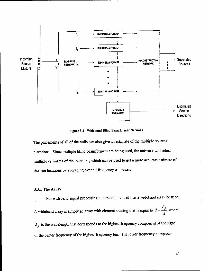
beamforming can be performed separately for each bin. Figure 3.2 shows the block

diagram for this wideband beamforming network. The output of all of the beamformers

will be sent through a reconstruction network where they will be combined to give an

estimate of the original signal.

40

Incoming * Source R

Mixture *

BANDPASS NETWORK '3 f,

>l BUND BEAMFORMER L

BUND BEAMFORMER

BLIND BEAMFORMER

» BUND BEAMFORMER

DIRECTION ESTIMATOR

RECONSTRUCTION NETWORK

Separated Sources

Estimated -> Source

Directions

Figure 3.2 - Wideband Blind Beamformer Network

The placements of all of the nulls can also give an estimate of the multiple sources'

directions. Since multiple blind beamformers are being used, the network will return

multiple estimates of the locations, which can be used to get a more accurate estimate of

the true locations by averaging over all frequency estimates.

3.3.1 The Array

For wideband signal processing, it is recommended that a wideband array be used.

Xf A wideband array is simply an array with element spacing that is equal to d = — where

Xfc is the wavelength that corresponds to the highest frequency component of the signal

or the center frequency of the highest frequency bin. The lower frequency components

41

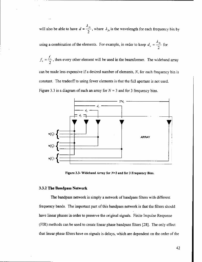
xf0 will also be able to have d = —, where Xf0 is the wavelength for each frequency bin by

using a combination of the elements. For example, in order to keep d0 = -J— for

/ f0 = —-, then every other element will be used in the beamformer. The wideband array

can be made less expensive if a desired number of elements, N, for each frequency bin is

constant. The tradeoff to using fewer elements is that the full aperture is not used.

Figure 3.3 is a diagram of such an array for N = 3 and for 3 frequency bins.

v(/-3)

v(£)

v(/i)

2* dx

u

rf2

— d. —\

i

f

1 r i >

r i r ▼

ARRAY

i

f \

» f i V

f 1 I

Figure 3.3- Wideband Array for JV=3 and for 3 Frequency Bins.

3.3.2 The Bandpass Network

The bandpass network is simply a network of bandpass filters with different

frequency bands. The important part of this bandpass network is that the filters should

have linear phases in order to preserve the original signals. Finite Impulse Response

(FIR) methods can be used to create linear phase bandpass filters [28]. The only effect

that linear phase filters have on signals is delays, which are dependent on the order of the

42

filters. The bandwidth of each filter can also increase with increasing center frequencies,

BWccfc.

3.3.3 The Blind Beamformers

The blind beamformers can now work independently on the bandpassed signals,

which are now considered narrowband signals. Since all of the filters are orthogonal in

the frequency domain, the beamforming can be done in parallel. The only difference

between the multiple beamformers is in the setup. Since beamformers for higher

frequencies have smaller element spacing compared to lower frequencies, the induced

delays due to propagation are smaller. The initial choice of delays should become

smaller and the step size parameters, ju and ß, should be set smaller to compensate for

this. This ensures stability for each beamformer and keeps the initial main beam

response the same for all the beamformers.

3.3.4 The Reconstruction Network

Since all of the outputs from the individual beamformers have no delays, the

reconstruction network is simply an adder. This is possible since the data from the

beamformers is orthogonal and therefore can be summed. If delays were introduced in

the network, then cross-correlation would need to be used to find the arbitrary delays.

43

3.3.5 The Direction Estimator

Since, the blind beamformers work by steering nulls in the direction of the

unwanted signals, it is therefore possible to estimate the direction of the signals by using

these null locations. The direction of the sources can be estimated by using the position

of the null that corresponds to the maximum from the other beam pattern. Since multiple

beamformers are being used for different frequency components, multiple estimates are

acquired from the beamformers. All of this information can be averaged together to get

estimate if the directions of the sources.

44

Chapter 4. Simulations and Results

4.1 Overview

In this chapter, results from many different types of simulations will be presented

and discussed. All simulations were conducted in MATLAB with a sampling rate of

88200 samples/second. All beamforming was done for a linear array in an azimuth plane.

The first section compares the advantages of using step size parameter control in the ICA

blind beamformer algorithm. The next section presents additional simulations including

a simulation for a mixture of three sources. Additional sections will explore the effects of

angle spacing between the sources, the performance for sources with unequal power

levels and the effects of additive noise on the algorithm. The last section presents a

simulation of a wideband directional noise signal and a wideband directional

communication signal.

4.2 Simulations

4.2.1 Simulations With and Without Step Size Parameter Control

The first simulation was set up for testing the adaptive algorithm, as presented in

Chapter 3, for narrowband signals. Two independent colored noise sources were made

with a bandwidth of 3250-3750 Hz. White noise sources were made with uniform

distributions and then bandpassed. The resulting sources had sub-Gaussian3 distributions.

The simulation was setup with j, (n) in the far field at an angle of+15° and s2 (n) in the

3 Sub-Gaussian Distributions are defined as having a longer tail compared to Gaussian distributions. They are also defined as having positive kurtosis.

45

far field at an angle of-15° perpendicular to the vertical array. The array had an element

spacing, d = 0.2m, which corresponds to half the wavelength of a 3750Hz sinusoidal

wave. A three-element array was used for the following simulations. The fixed beam

pattern without steering is shown in Figure 4.1. The signal to interference ratio (SIR) for

a fixed beam pattern with a maximum at 0° is OdB for both sources since both signals

vai(signal) were set with equal variances, where SIR

vai(interference)

Figure 4.1 - Fixed Beam Pattern for a Three-Element Array.

The first simulation was performed by using the algorithm in Equation 3.17. The

step size parameters were set to ßp{n) = 0.01 and ßp(ri) = 0.01. The BSS step size

parameter, JUBSS, for this simulation and for all of the following simulations was set to

MBSS = 0.0005. The learning curve for this simulation is shown in Figure 4.2a. The

ending delays were found to be d] = -5 and d2 = +5. As can be seen in the plot, the

delays did not converge until approximately 15,000 iterations. Today, with dedicated

46

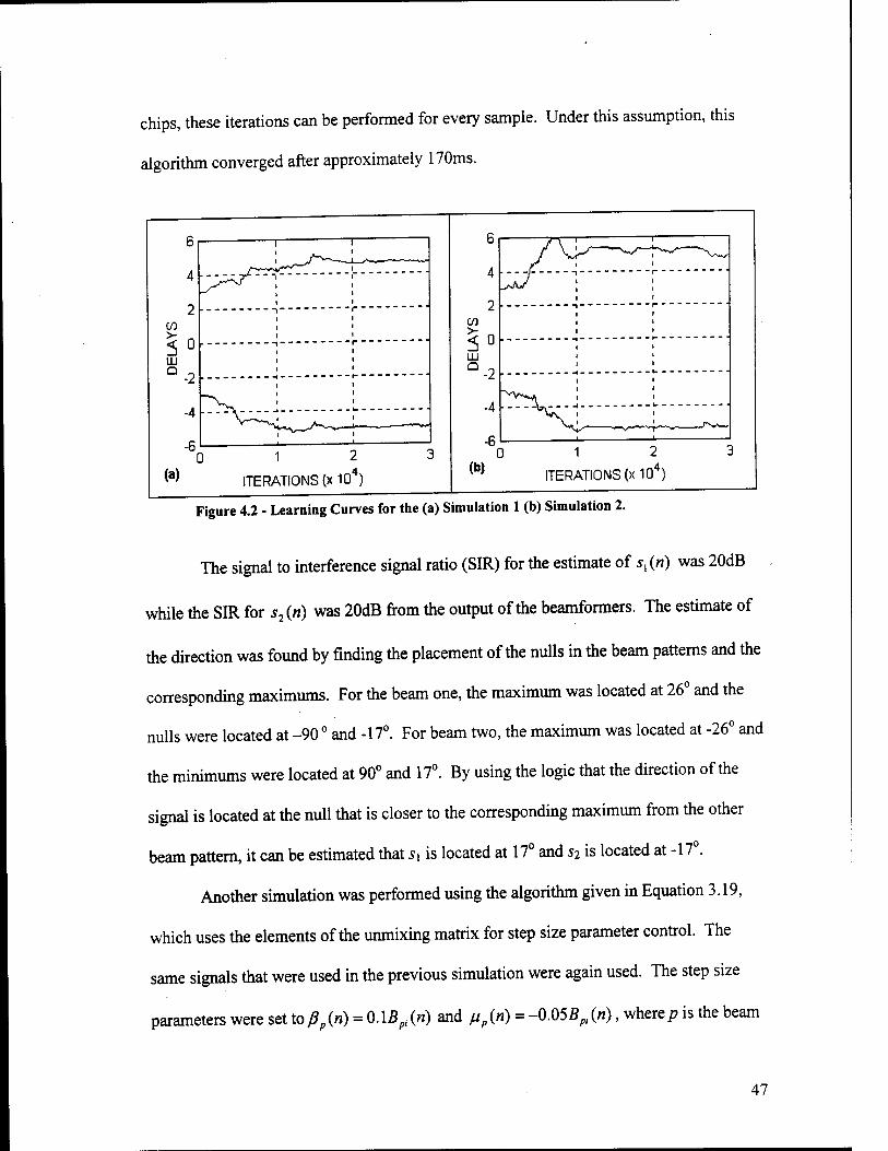
chips, these iterations can be performed for every sample. Under this assumption, this

algorithm converged after approximately 170ms.

ITERATIONS (x 10 )

6

4

2 CO

HI

°-2

-4

-6

(b)

-i r

1---------T

_4____-----t-

1 2

ITERATIONS (x 104)

Figure 4.2 - Learning Curves for the (a) Simulation 1 (b) Simulation 2.

The signal to interference signal ratio (SIR) for the estimate of j, («) was 20dB

while the SIR for j2 («) was 20dB from the output of the beamformers. The estimate of

the direction was found by finding the placement of the nulls in the beam patterns and the

corresponding maximums. For the beam one, the maximum was located at 26° and the

nulls were located at -90 ° and -17°. For beam two, the maximum was located at -26° and

the minimums were located at 90° and 17°. By using the logic that the direction of the

signal is located at the null that is closer to the corresponding maximum from the other

beam pattern, it can be estimated that s\ is located at 17° and s2 is located at -17°.

Another simulation was performed using the algorithm given in Equation 3.19,

which uses the elements of the unmixing matrix for step size parameter control. The

same signals that were used in the previous simulation were again used. The step size

parameters were set to ßp (») = 0. \Bpi (n) and //, (») = -0.055,, (»), where p is the beam

47

number, and Bpt (n) is a non-diagonal element from the unmixing matrix, B, at time n.

The learning curve for the algorithm is shown in Figure 4.2b. As can be seen in the plot,

the delays converged after approximately 10,000 iterations (114ms), which was an

improvement compared to above. The ending delays were found to bed, = -5 and

d2 = +5.

The SIR for the estimate of sx (n) was 20dB while the SIR for s2 (n) was 20dB.

These numbers do not reflect the additional gain that the BSS algorithm provided. The

SIR including the effects of BSS resulted in an average SIR of s,(w) is 30dB while the

SIR for 52 (w) is 30dB. This is a large improvement compared to the SIR that resulted in

the fixed beam pattern. Figure 4.3 shows a plot of the windowed SIR for the output of

the beamformers and the BSS algorithm. It can be seen that the SIR ratio increased much

quicker for the BSS outputs than the beamformer outputs. Even though the delays did

not converge until approximately 10,000 iterations (113ms), the SIR improved to above

15dB after 3000 iterations (34ms). For this situation the BSS algorithm not only helped

steer the beams, but it also provided additional SIR gain.

48

50

40

CD S30 er

20

10

—f\rf-\ "T / > ' '

■S--r * - ■; -

(a)

1 24 3

ITERATIONS (x 10*)

- - W/out BSS — W/BSS

50

40

S 30

CO 20

10 ./ /I 4. 1

1 2 ITERATIONS (x 104)

(M

• W/out BSS •W/BSS

Figure 4.3 - Plot of SIR for (a) Beam 1 and (b) Beam 2 for Simulation 2.

The directions of the sources were again found using the same method as before.

For beam one, the maximum was located at 26° and the minimums were located at -90

and -17°. For the beam two, the maximum was located at -26° and the minimums were

located at 90 and 17°. By using the same logic as before, it can be estimated that s\ is

located at 17° and s2 is located at -17°, which were again accurate.

A plot of the resulting step size parameter, ///(«), is shown in Figure 4.4 for both

simulations. It can be seen that jui(n) was large when the delays were far from the

optimum solution and was set smaller when the delays were near optimum. The same

thing happened for the other step size parameters, fifct). In the first simulation, the step

size parameters were set to constants.

49

Figure 4.4 - Step Size Parameter, Mt(n), for Simulation 1 and Simulation 2.

It was shown in the previous simulations that both methods converged properly.

Both simulations demonstrated large improvements in SIR compared to fixed

beamforming. It was also shown that the second method as presented Chapter 3.2.4,

which used adjustable step size parameters, sped up convergence and required less

computing power. For the rest of this thesis, all additional simulations will use the

adjustable step size parameters.

3.2.2 Additional Simulations

A third simulation was performed with the sources in different locations. This

simulation used the same sources as above with s{ (n) in the far field at an angle of +37°

and s2 (n) in the far field at an angle of 0° perpendicular to the vertical array. The array

again had an element spacing, d = 0.2m, which corresponds to half the wavelength of a

3750Hz wave. The step size parameters were set to ßp («) = 0. \Bpi (n) and

50

jj (M) = -0.055 , (n), where p is the beam number, and Bpi («) is the non-diagonal

elements from the unmixing matrix, B. The SIR of the sources for a fixed beam pattern

with a maximum at 0° is SIR = 12dB for sx («) and SIR = -12dB for s2 (n).

The learning curve for the algorithm is shown in Figure 4.5(a). As can be seen in

the plot, the delays converged after approximately 20,000 iterations (227ms). The ending

delays were found to be^ = -9 and d2 = +2. The SIR for the estimate of sx (n) for the

ending delays was 22dB while the SIR for s2 («) was 21 dB. This was a large

improvement for both signals compared to the SIR for fixed beamforming.

ITERATIONS (x 10 )

0.03

HI tD 0.02 i £ o.oi

CO

UJ u

i- w

-0.01

T 1 1

.J 1 T

Ufr- - -r — - T

i i ] i K j - - ^ . J- - .1 - * - * -.- - .4 W

(b) 1 2 43 ITERATIONS (x 10 )

Figure 4.5 - (a) Learning Curves and (b) Step Size Parameter, n,(h), for Simulation 3.

Figure 4.6 shows a plot of the SIR over iteration time for both outputs. It can be seen that

BSS did not improve the estimate of s, («) in early iterations, but it did improve the

estimate of s2 (n) for almost all iterations.

51

m

35

30

25

S 20

15

10

5 1 ITERATIONS (x 10

(a)

- - W/out BSS

— W/BSS

40

30

m 20 ■a

CC C/D 10

-10

1— T—- ,

1 ITERATIONS (x 10 )

(b)

■ W/out BSS

■W/BSS

Figure 4.6 - Plot of SIR for (a) Beam 1 and (b) Beam 2 for Simulation 3.

The algorithm also provided an estimate of positions of the sources. For the beam

one, the maximum was located at 51° and the minimums were located at 6° and -34°. For

beam two, the maximum was located at -10° and the minimums were located at 31 and

-57°. A plot of these beams can be seen in Figure 4.7. It can again be estimated that s\ is

located at 31° and 52 is located at 6°.

90 0.99994 60

90 0.99998

Figure 4.7 - Beam Patterns for (a) Beam 1 and (b) Beam 2.

52

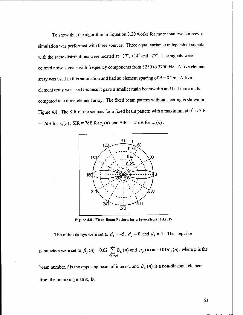
To show that the algorithm in Equation 3.20 works for more than two sources, a

simulation was performed with three sources. Three equal variance independent signals

with the same distributions were located at +37°, +14° and -27°. The signals were

colored noise signals with frequency components from 3250 to 3750 Hz. A five element

array was used in this simulation and had an element spacing of d = 0.2m. A five-

element array was used because it gave a smaller main beamwidth and had more nulls

compared to a three-element array. The fixed beam pattern without steering is shown in

Figure 4.8. The SIR of the sources for a fixed beam pattern with a maximum at 0° is SIR

= -7dB for $,(»), SIR = 7dB fors2(«) and SIR = -21 dB for s3(n).

Figure 4.8 - Fixed Beam Pattern for a Five-Element Array

The initial delays were set to dx = -5, d2 = 0 and d3= 5. The step size

parameters were set to ßp (w) = 0.02 £ \Bpi (n)\ and npi (n) = -0.0\Bpi (»), where p is the /=I(/*P)

beam number, i is the opposing beam of interest, and Bpi(n) is a non-diagonal element

from the unmixing matrix, B.

53

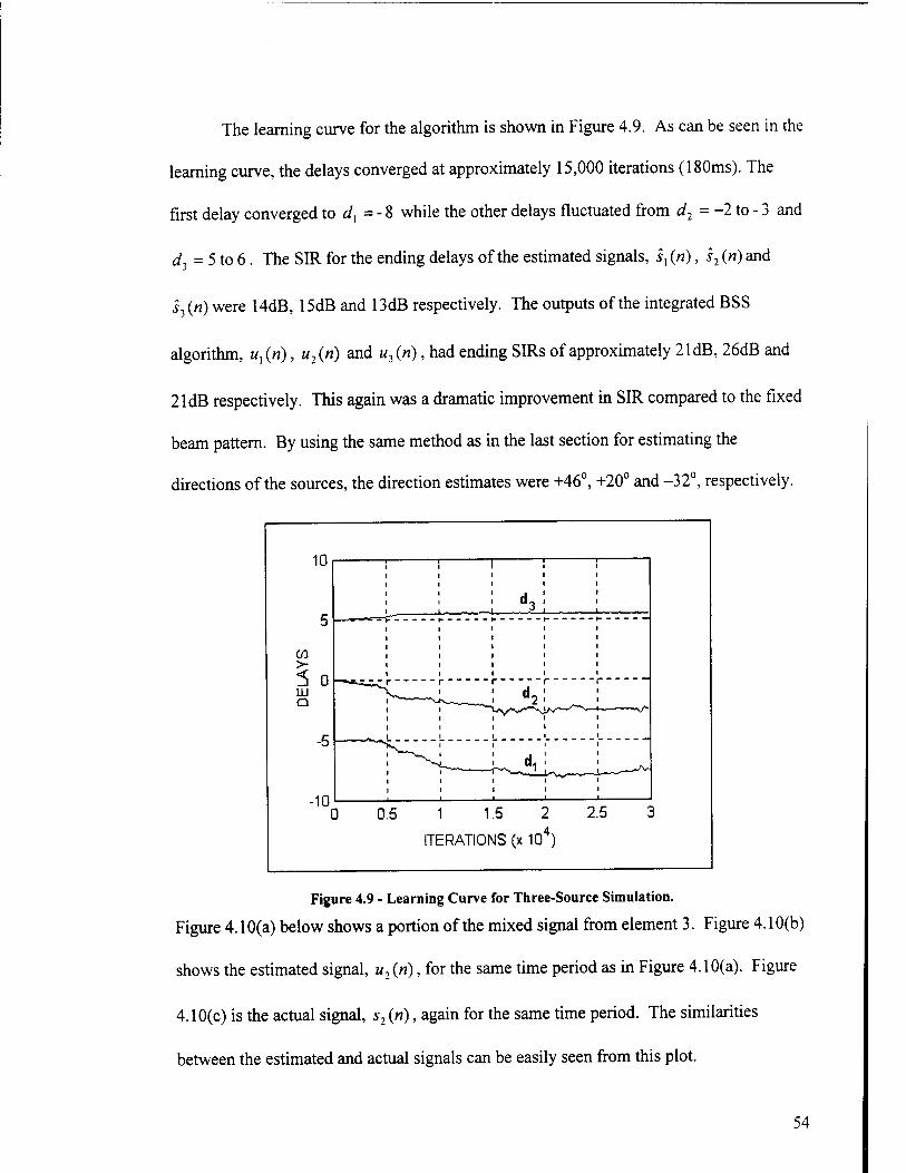
The learning curve for the algorithm is shown in Figure 4.9. As can be seen in the

learning curve, the delays converged at approximately 15,000 iterations (180ms). The

first delay converged to dx = - 8 while the other delays fluctuated from d2 = -2 to - 3 and

d3 = 5 to 6. The SIR for the ending delays of the estimated signals, s, («), s2 (n) and

£3(w) were 14dB, 15dB and 13dB respectively. The outputs of the integrated BSS

algorithm, «,(«), u2{n) and w3(«), had ending SIRs of approximately 21 dB, 26dB and

21 dB respectively. This again was a dramatic improvement in SIR compared to the fixed

beam pattern. By using the same method as in the last section for estimating the

directions of the sources, the direction estimates were +46°, +20° and -32°, respectively.

0 0.5 1 1.5

ITERATIONS (x 10 )

Figure 4.9 - Learning Curve for Three-Source Simulation.

Figure 4.10(a) below shows a portion of the mixed signal from element 3. Figure 4.10(b)

shows the estimated signal, u2{n), for the same time period as in Figure 4.10(a). Figure

4.10(c) is the actual signal, s2 (n), again for the same time period. The similarities

between the estimated and actual signals can be easily seen from this plot.

54

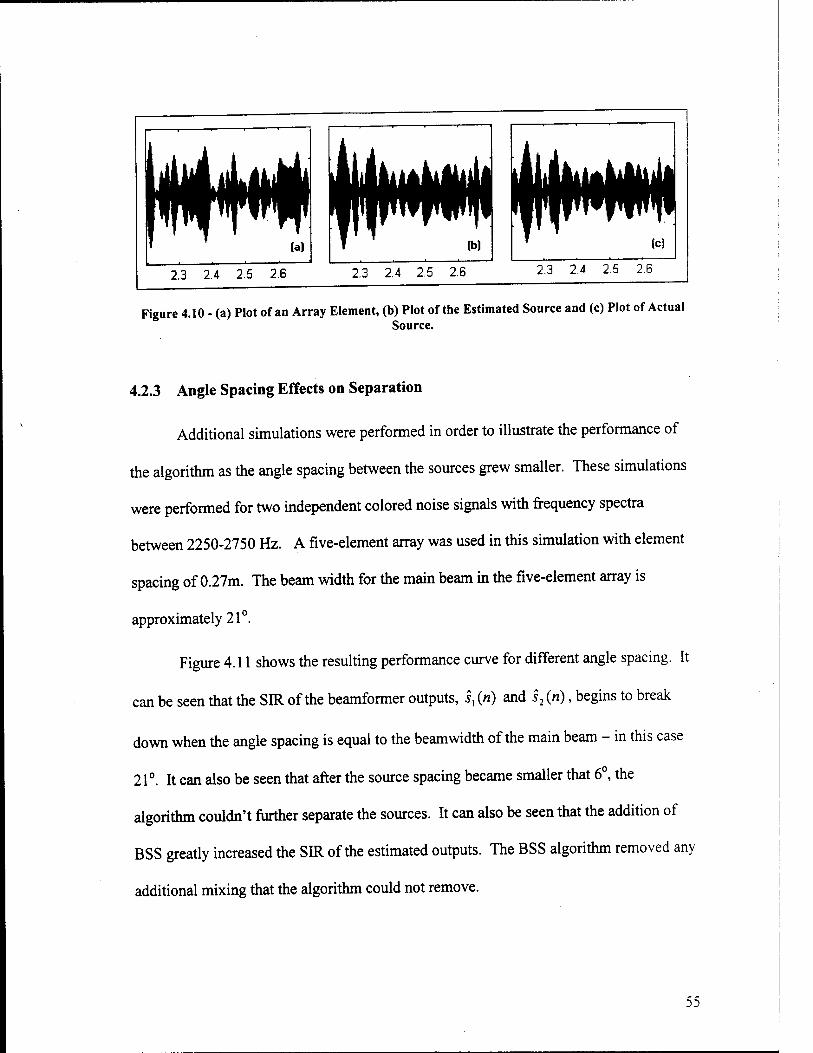
2.3 2.4 2.5 2.6 2.3 2.4 2.5 2.6 2.3 2.4 2.5 2.6

Figure 4.10 - (a) Plot of an Array Element, (b) Plot of the Estimated Source and (c) Plot of Actual Source.

4.2.3 Angle Spacing Effects on Separation

Additional simulations were performed in order to illustrate the performance of

the algorithm as the angle spacing between the sources grew smaller. These simulations

were performed for two independent colored noise signals with frequency spectra

between 2250-2750 Hz. A five-element array was used in this simulation with element

spacing of 0.27m. The beam width for the main beam in the five-element array is

approximately 21°.

Figure 4.11 shows the resulting performance curve for different angle spacing. It

can be seen that the SIR of the beamformer outputs, i, («) and s2 («), begins to break

down when the angle spacing is equal to the beamwidth of the main beam - in this case

21°. It can also be seen that after the source spacing became smaller that 6°, the

algorithm couldn't further separate the sources. It can also be seen that the addition of

BSS greatly increased the SIR of the estimated outputs. The BSS algorithm removed any

additional mixing that the algorithm could not remove.

53

40

30

.20

10

-10

—1 1 1— 1

1 1 1 1/

; ; ; /;

> ^ ^.

"1 i y—J-y ! ! \ i \ /

\ r~\' /\

5 10 15 20 25 30

ANGLE SPACING (DEG)

— Output ot Beamformer

-- Output o< BSS Algorlhm

Figure 4.11 - SIR of the Output from Beam 1 vs. the Angle Separation of the Sources.

4.2.4 Performance for Sources with Unequal Power Levels

All of the above simulations were performed for sources with equal power levels.

This section explores the performance of the algorithm for sources with different power

levels. These simulations were performed for two independent colored noise signals

located at +14 and -14 with frequency spectra between 3250-3750 Hz. A three-element

array was used in this simulation with element spacing of 0.2m.

Figure 4.12(a) shows a plot of the SIR improvement from the ICA blind

beamformer for SIR ratios of the original sources. It can be seen that the most SIR

improvement from the algorithm came when the SIR was near OdB. It can also be seen

that the algorithm did more to improve signals that had the least power than signals that

had the most power. This occurs because the algorithm can easily place a null in the

direction of a high power source because the gradient is large. It was more difficult for

the algorithm to null out the sources with less power because the beam already had very

small amounts of the opposing signal. Because of this, the gradient was very small which

56

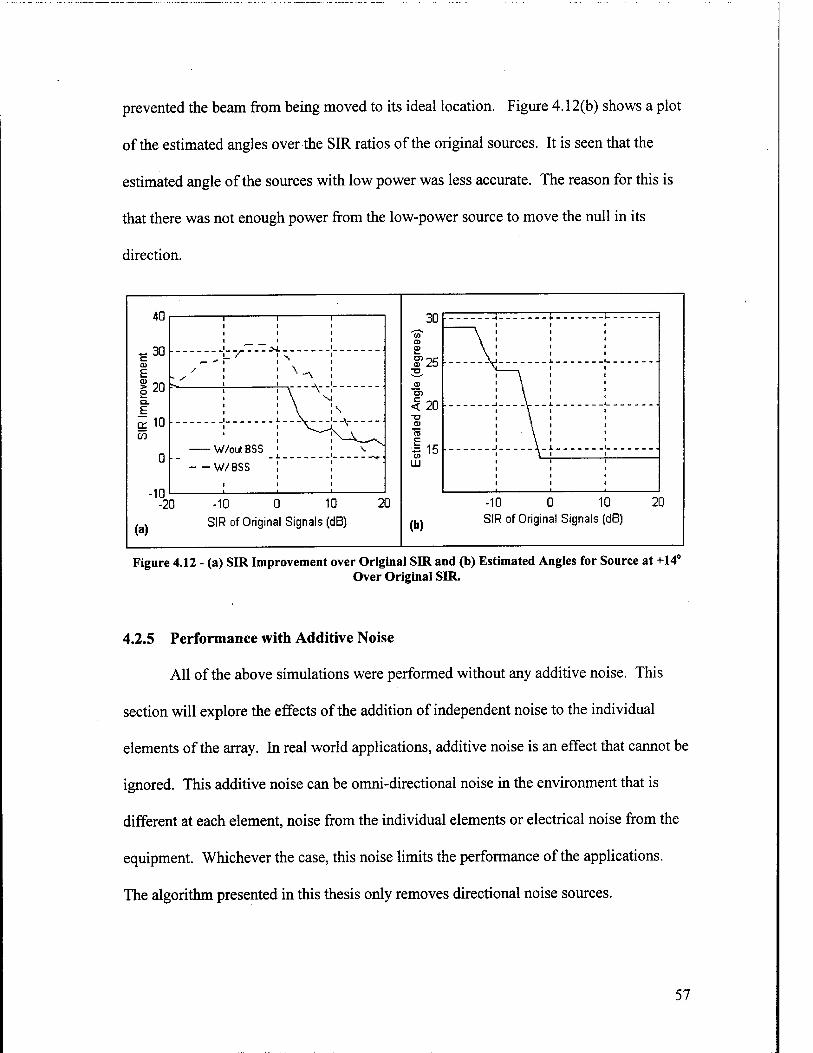
prevented the beam from being moved to its ideal location. Figure 4.12(b) shows a plot

of the estimated angles over the SIR ratios of the original sources. It is seen that the

estimated angle of the sources with low power was less accurate. The reason for this is

that there was not enough power from the low-power source to move the null in its

direction.

-20

(a)

-10 0 10

SIR of Original Signals (dB)

30 *—•■. (0 a> 0)

ST 25

< 20

i« LU

(b)

_| *.

J J.

-I \ i.

J 1-1

-10 0 10 SIR of Original Signals (dB)

20

Figure 4.12 - (a) SIR Improvement over Original SIR and (b) Estimated Angles for Source at +14° Over Original SIR.

4.2.5 Performance with Additive Noise

All of the above simulations were performed without any additive noise. This

section will explore the effects of the addition of independent noise to the individual

elements of the array. In real world applications, additive noise is an effect that cannot be

ignored. This additive noise can be omni-directional noise in the environment that is

different at each element, noise from the individual elements or electrical noise from the

equipment. Whichever the case, this noise limits the performance of the applications.

The algorithm presented in this thesis only removes directional noise sources.

57

Many simulations were performed for this section with different levels of additive

noise. The additive noise used in this section was white Gaussian noise (WGN) with zero

mean. The directional signals were again colored noise with frequency components

again from 3275-3750Hz. Source one was located at -37° and source two was located at

0°. Before the data was sent through the blind beamforming algorithm, the data was

bandpassed to remove the effects of the noise outside of the band. Figure 4.13(a) shows a

plot of the signal to interfering signal ratio (SIR) of both signals over different signal to

noise ratios (SNR) of the additive noise. The SNR is the ratio of the variance of the

bandpassed noise signal added to one element over the variance of one of the original

sources. The performance of the algorithm continually declines over all SNRs. Figure

4.13(b) shows a plot of the signal to noise and interference ratio (SNIR) or both signals

var(signal) and the theoretical bound. The SNIR is defined as SNIR

vai(noise) + var(interference)

A constant decrease is shown and is expected because no attempt is made to remove the

effects of the additive noise.

10 o SNR (dB)

(a) 1,(37°)

20

10

0) 0 UJ

a. -10 z

■20

5i^' i :

20 10 0 SNR (dB)

-10

(b) s2(37°) Best Theoretical Vakje

Figure 4.13 - (a) SIR between Opposing Signals vs. Additive Noise Levels and (b) SNIR of Estimated Signals vs. Additive Noise Levels.

58

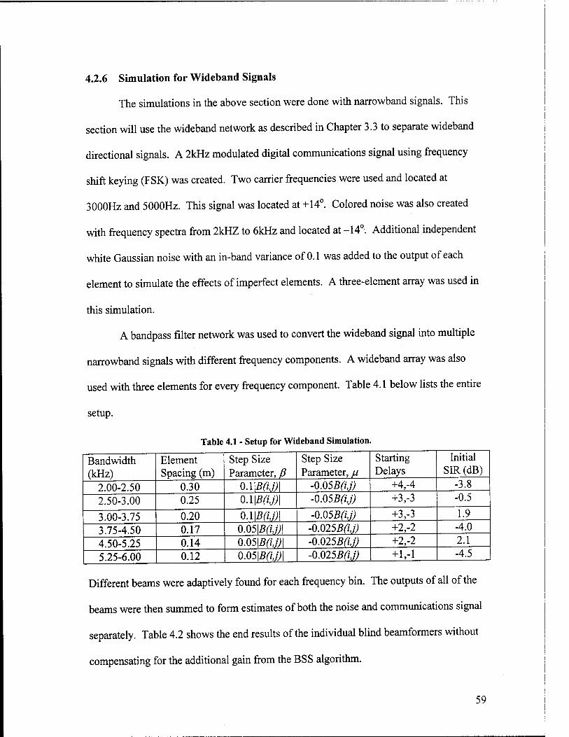
4.2.6 Simulation for Wideband Signals

The simulations in the above section were done with narrowband signals. This

section will use the wideband network as described in Chapter 3.3 to separate wideband

directional signals. A 2kHz modulated digital communications signal using frequency

shift keying (FSK) was created. Two carrier frequencies were used and located at

3000Hz and 5000Hz. This signal was located at +14°. Colored noise was also created

with frequency spectra from 2kHZ to 6kHz and located at -14°. Additional independent

white Gaussian noise with an in-band variance of 0.1 was added to the output of each

element to simulate the effects of imperfect elements. A three-element array was used in

this simulation.

A bandpass filter network was used to convert the wideband signal into multiple

narrowband signals with different frequency components. A wideband array was also

used with three elements for every frequency component. Table 4.1 below lists the entire

setup.

Table 4.1 - Setup for Wideband Simulation.

Bandwidth (kHz)

Element Spacing (m)

Step Size Parameter, ß

Step Size Parameter, ju

Starting Delays

Initial SIR (dB)

2.00-2.50 0.30 0.1 B(iJ)\ -0.05B(ij) +4,-4 -3.8

2.50-3.00 0.25 0.1\B(ij)\ -0.05B(i,j) +3,-3 -0.5

3.00-3.75 0.20 O.lBflJ) -0.05B(ij) +3,-3 1.9

3.75-4.50 0.17 0.05 Bfij) -0.025B(ij) +2,-2 -4.0

4.50-5.25 0.14 0.05WJ) -0.025B(i,j) +2,-2 2.1

5.25-6.00 0.12 0.05 B(i,j)\ -0.025B(i,j) +1,-1 -4.5

Different beams were adaptively found for each frequency bin. The outputs of all of the

beams were then summed to form estimates of both the noise and communications signal

separately. Table 4.2 shows the end results of the individual blind beamformers without

compensating for the additional gain from the BSS algorithm.

59

Table 4.2 - Results From Wideband Network.

Bandwidth (kHz)

Delay 1, d,

Delay 2, d2

Estimated Direction of Beam 1

Estimated Direction of Beam 2

SIR Beam l(dB)

SIR Beam 2 (dB)

2.00-2.50 -5 8 23 -13 12 14 2.50-3.00 -6 6 15 -15 16 14 3.00-3.75 -6 4 19 -9 17 12 3.75-4.50 -3 5 10 -21 14 15 4.50-5.25 -4 3 18 -11 25 14 5.25-6.00 -2 3 7 -15 14 17 2.00-6.00 - - 15 -14 14 14

The estimates of the locations were very accurate. Additional gain came from the BSS

algorithm. This gain can be found in Table 4.3.

Table 4.3 - SIR for Algorithms With and Without BSS.

Bandwidth (kHz)

SIR Beam 1 (dB)

SIR Beam 1 (dB)

SIR Beam 1 (dB) (w/ BSS)

SIR Beam 2 (dB) (w/ BSS)

2.00-2.50 12 14 19 21 2.50-3.00 16 14 26 26 3.00-3.75 17 12 14 25 3.75-4.50 14 15 17 15 4.50-5.25 25 14 22 16 5.25-6.00 14 17 16 20 2.00-6.00 14 14 17 18

From the table above, it can be shown that integrated BSS increased the SIR for both the

noise and the communications signal. The SIR of the noise signal estimate increases by

3dB and the SIR of the communications signal increased by 4dB.

The output signals were found to be independent as expected. Figure 4.14(a,b)

shows plots of the linear and non-linear cross-correlation between both beam outputs and

similar plots between the original signals. It can be seen that the beam outputs become

more independent as the number of iterations increase. Figures 4.14(c,d) show plots of

the nonlinear cross correlation between the original signals and the estimated signals. It

can be seen that after approximately 4000 iterations (45ms), the estimated signals

60

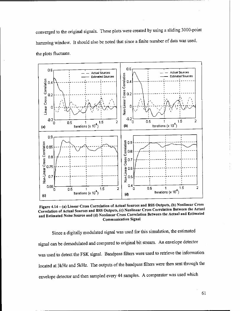
converged to the original signals. These plots were created by using a sliding 3000-point

hamming window. It should also be noted that since a finite number of data was used,

the plots fluctuate.

0.6

I 0.4

o 0.2

o

-0.2

1 i

Actual Sources

I

1

1

A 1

i

i_ i

0.5 (a)

1 Iterations (x 10H)

1.5

0.6 c o IS £ 0.4 o o v>

8 0.2 o

-0.2

i—— i

Actual Sources

1

1 1

1

■-fk f\ / <\* ' '

i i

0.5 (b)

1 Iterations (x 10*)

1.5

0.9

tS0.85

o

o

0.8

0.75

0.7

0.65

j , ,

I I '

0.5

(c)

1 Iterations (x 10*)

1.5

Non

-Lin

ear

Cro

ss C

orre

latio

n D

CD

p

P

p

P

0.5

w 1

Iterations (x 10*) 1.5

Figure 4 14 - (a) Linear Cross Correlation of Actual Sources and BSS Outputs, (b) Nonlinear Cross Correlation of Actual Sources and BSS Outputs, (c) Nonlinear Cross Correlation Between the Actual and Estimated Noise Source and (d) Nonlinear Cross Correlation Between the Actual and Estimated

Communication Signal

Since a digitally modulated signal was used for this simulation, the estimated

signal can be demodulated and compared to original bit stream. An envelope detector

was used to detect the FSK signal. Bandpass filters were used to retrieve the information

located at 3kHz and 5kHz. The outputs of the bandpass filters were then sent through the

envelope detector and then sampled every 44 samples. A comparator was used which

61

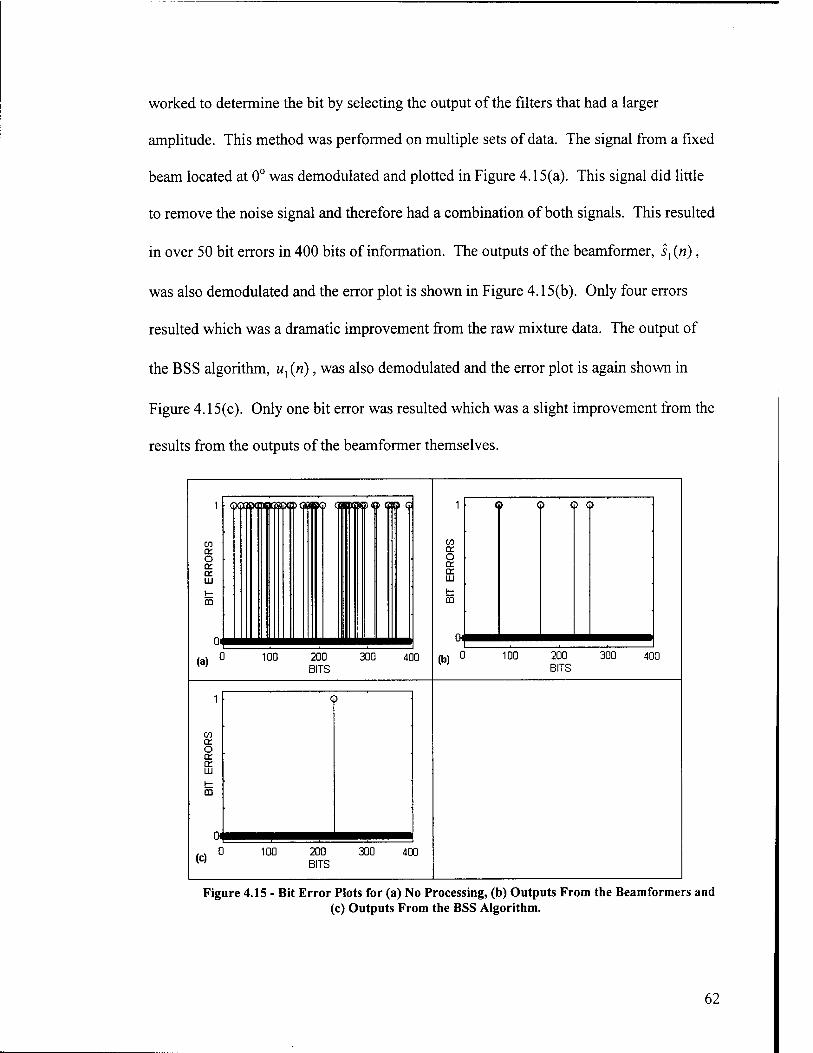
worked to determine the bit by selecting the output of the filters that had a larger

amplitude. This method was performed on multiple sets of data. The signal from a fixed

beam located at 0° was demodulated and plotted in Figure 4.15(a). This signal did little

to remove the noise signal and therefore had a combination of both signals. This resulted

in over 50 bit errors in 400 bits of information. The outputs of the beamformer, s, («),

was also demodulated and the error plot is shown in Figure 4.15(b). Only four errors

resulted which was a dramatic improvement from the raw mixture data. The output of

the BSS algorithm, w, (ri), was also demodulated and the error plot is again shown in

Figure 4.15(c). Only one bit error was resulted which was a slight improvement from the

results from the outputs of the beamformer themselves.

400

1 < >

w o a: HI

t- m

■

(c) 100 200

BITS 300 400

to en o ce a. LU

t on

(b)

a a a a

100 200 BITS

300 400

Figure 4.15 - Bit Error Plots for (a) No Processing, (b) Outputs From the Beamformers and (c) Outputs From the BSS Algorithm.

62

4.2 Conclusions

The algorithm as presented in Equation 3.18 was shown to work for various

situations. Many simulations were performed on narrowband signals with different

locations. All of these simulations resulted in accurate estimates of the original signals

and of their directions. The algorithm showed strong levels of noise immunity and was

shown to separate signals that were separated by only 6° using a five-element array.

Another simulation was performed on two wideband signals propagating from different

directions. The wideband network, as discussed in Chapter 3.3, was used and performed

well in separating the signals. The directions of the sources were again found and

estimates of the signals were found to be relatively clean. It should be noted that this

thesis did not focus on speeding up the convergence time; however, it did speed up the

separation process by utilizing BSS.

63

Chapter 5. Conclusions and Future Work

5.1 Future Work

The algorithm that was presented in this thesis worked for sources that were

statistically independent. However, in many underwater environments, these signals may

not be independent since some of these signals can be reflections of each other. If the

signals are reflected, then they will appear to be propagating from different directions. It

can sometimes be assumed that the time differences between the reflections and the

original signal are larger than the correlation time of the signals. If this assumption is

true, then the signals will appear statistically independent. This assumption, however,

may not be always true. It is possible that multiple reflections occur and arrive at the

array at the same time. If this happens then the algorithm will be confused and may not

adapt correctly. Additional work can be continued in order to address this problem.

Another possible research area for a continuation of this thesis is to improve the

algorithm to allow the element weights to be adapted along with the element delays. This

could possibly increase performance and possibly speed up convergence. This can also

be taken a step further by using the narrowband assumption and adjust complex weights

instead of delays. This would become less complex because derivatives would not need

to be calculated. The sampling rate could also be smaller compared with time-delay

beamforming because phase shifts are used instead of time shifts. Consideration must be

made in this continuation to make sure that no delays are formed in this process, which

can create an artificial independence.

64

5.2 Conclusions

The problem that was addressed in this thesis was to separate unknown

independent signals that propagate from unknown directions. The goal of this thesis was

to develop an algorithm to find these unknown directions and return an estimate of the

corresponding unmixed signals. It was shown that current algorithms did not solve this

problem of separating multiple signals and finding their directions when no a priori

knowledge is known about the signal waveforms and their directions. Some of these

algorithms used specific assumptions about the sources such as cyclostationarity and

constant modulus. These assumptions cannot be applied to unknown passive sources,

since this information is unknown. Some of these algorithms worked by using power as a

criterion, which worked to find the signal with the most power, but did not separate

multiple signals. Other algorithms were developed to estimate the signals, but did not

estimate their directions. The algorithm presented in this thesis was a continuation of

many of these methods and was designed to solve the problem as stated above.

Preliminary work has demonstrated that the algorithm successfully separated

signals when no a priori information was known about the sources waveforms and their

directions. It was also shown that the incorporation of BSS improved convergence time

and also improved the SIR of the estimated signals. A wideband network was also used

successfully to expand the algorithms to work with wideband signals. Overall, this

algorithm has shown great promise in solving the problem of blind beamforming for

unknown passive sources.

65

References

[I] L.C. Godara and D.B. Ward, "A General Framework for Blind Beamforming," TENCON 99, Proceedings of the IEEE Region 10 Conference, Vol. 2, pp. 1240-1243, 1999.

[2] S. Choi, and D. Yun, "Design of an Adaptive Antenna Array for Tracking the Source of Maximum Power and Its Application to CDMA Mobile Communications," IEEE Transactions on Antennas and Propagation, Vol. 45, pp. 1393-1404, Sept. 1997.

[3] Q. Wu and K.M. Wong, "Blind Adaptive Beamforming for Cyclostationary Signals," IEEE Trans. Signal Processing, Vol. 44, pp. 2757-5767, Nov 1996.

[4] A. Van Der Veen and A. Paulraj, "An Analytical Constant Modulus Algorithm,' IEEE Trans. Signal Processing, Vol. 44, pp. 1136-1155, Apr. 1996.

[5] A. Papoulis, Probability, Random Variables, and Stochastic Processes, WCB McGraw Hill, Boston, 1991.

[6] W. S. Burdic, Underwater Acoustic System Analysis, Prentice-Hall, Inc., New Jersey, 1991.

[7] D. H. Johnson and D.E. Dudgeon, Array Signal Processing: Concepts and Techniques, Prentice Hall, New Jersey, 1993.

[8] R.A. Monzingo and T.W. Miller, Introduction to Adaptive Arrays, Wiley Interscience, New York, 1980.

[9] B. Widrow and S.D. Stearns, Adaptive Signal Processing, Prentice Hall, 1985.

[10] B.D. Steinberg, Principles of Aperture and Array System Design, Wiley, New York, 1976.

[II] S. Haykin, Adaptive Filter Theory, Prentice-Hall, New Jersey, 1996.

[12] B. Widrow, P.E. Mantey, L.J. Griffiths, and B.B. Goode, "Adaptive Antenna Systems", Proc. IEEE, Vol. 55, pp. 2143-2159, Dec. 1967.

[13] R.T. Compton, Jr., Adaptive Antennas, Prentice Hall, New Jersey, 1988.

[14] J. Cardosa and A. Souloumiac, "Blind Beamforming for Non-Gaussian Signals, IEE Proceedings F, Vol 36, pp. 287-314,1994.

66

[15] A. Wax and Y. Arm, "A Least Squares Approach to Blind Beamforming," IEEE Transactions on Signal Processing, Vol. 47, pp. 231-234, Jan. 1999.

[16] J. Sheinvald, "Blind Beamforming for Multiple Non-Gaussian Signals and the Constant-Modulus Algorithm," IEEE Transactions on Signal Processing, Vol. 46, pp. 1878-1885, July 1998.

[17] C.S. Tsang and R.T. Compton, "A Time Delay Algorithm for Adaptive Arrays," Aerospace Applications Conference, Proc. IEEE, Vol. 4, pp. 457-468, 1996.

[18] J. Herault and C. Jutten, "Space or Time Adaptive Signal Processing by Neural Network Models," Neural Networks for Computing, AIP Conf, Proc, Vol. 151, pp. 207- 211, Snowbird, UT, 1986.

[19] A.J. Bell and T.J. Sejnowski, "An Information-Maximization Approach to Blind Separation and Blind Deconvolution," Neural Computation, Volume 7, pp. 1129-1159, 1995.

[20] S. Amari and H.H. Yang, "A Stochastic Natural Gradient Descent Algorithm for Blind Signal Separation," Neural Networks for Signal Processing [1996] VI, pp. 433 - 442, 1996.

[21] T. M. Cover and J. A. Thomas, Elements of Information Theory, John Wiley & Sons, New York, 1991.

[22] S. Li and T.J. Sejnowski, "Adaptive Separation of Mixed Broad-Band Sound Sources with Delays by a Beamforming Herault-Jutten Network," IEEE Journal of Oceanic Engineering, Vol. 20, pp. 73-79, Jan. 1995.

[23] K. Torkkola, "Blind Separation of Delayed Sources Based on Information Maximization," Proceedings of the IEEE International Conference on Acoustic, Speech and Signal Processing, Vol. 6, pp. 3509-3512, Atlanta, GA, 1996.

[24] S. Armari and A. Cichocki, "Adaptive Blind Signal Processing - Neural Network Approaches," Proceedings of the IEEE, Vol. 86, pp. 2026-2048, Oct. 1998.

[25] J. Cardosa, "Blind Signal Separation: Statistical Principles," Proceedings of the IEEE, Vol. 86, pp. 2009-2025, Oct. 1998.

[26] K. Torkkola, "Blind Separation of Convolved Sources Based on Information Maximization'", Neural Networks for Signal Processing, Vol. 6, Kyoto, Japan, 1996.

[27] P. Smaragdis, "Blind Separation of Convolved Mixtures in the Frequency Domain," International Workshop on Independence & Artificial Neural Networks University of La Laguna, Tenerife, Spain, February 9-10, 1998.

67

[28] A. W. Oppenheim and R. W. Schäfer, Digital Signal Processing, Prentice-Hall, New Jersey, 1975.

68