An Incremental Constraint Solver - Georgia Institute of … Incremental Constraint Solver An incremental constraint solver, the DeltaBlue algorithm maintains an evolving solution to

SPECIAL SECTION

An Incremental Constraint Solver

An incremental constraint solver, the DeltaBlue algorithm maintains an evolving solution to the constraint hierarchy as constraints are added and removed. DeltaBlue minimizes the cost of finding a new so1utio.n after each change by exploitin!;g its knowledge of the last solution.

Bjorn N. Freeman-Benson, John Maloney, and Alan Borning

A constraint describes a relation that should be satisfied. Examples of constraints include:

l a constraint that a line on a computer display be vertical

l a constraint that a resistor in a circuit simulation obey Ohm’s Law

l a constraint that two views of the same data remain consistent (for example, bar graph and pie chart views).

Constraints are useful in programming languages, user interface toolkits, simulation packages, and other systems because they allow programmers or users to state declaratively a relation that is to be maintained, rather than requiring them to write procedures to maintain the relation themselves. Constraints are nor- mally multidirectional. For example, a constraint that c = II + b might be used to find a value of one of a, b, or c. In general there may be many interrelated constraints in a given application; it is left up to the system to sort out how they interact and to keep them all satisfied.

In many applications, it is useful to be able to state both required and preferential constraints. The required constraints must hold. The system should try to satisfy the preferential constraints if possible, but no error condition arises if it can not. In the work presented here, we allow an arbitrary number of levels of preference, each successive level being more weakly preferred than the previous one. The set of all constraints, both required and preferred, labeled with their respective strengths, is called a constraint hierarchy.

As one example of using constraint hierarchies, consider the problem of laying out a table in a document. We would like the table to fit on a single page while still leaving adequate white space between rows. This can be represented as the interaction of two constraints:

Bjorn Freeman-Benson and John Maloney were supported by fellowships from the National Science Foundation and Apple Computer respectively. This project was supported in part by the National Science Foundation under Grant Number IRI-8803294, by Apple Computer and by the Washington Tech- nology Center.

0 1990 ACM OOOl-0782/90/0100-0054 $1.50

54 Communications of the ACM

a required constraint that the height of the blank space between lines be greater than zero, and a preferred constraint that the entire table fit on one p,age. As another example, suppose we are moving a part of a constrained geometric figure around on the display using the mouse. While the part moves, other pa:rts may also need to move to keep all the constraints satisfied. How- ever, if the locations of all parts are not determined, we would prefer that they remain where they were, rather than flailing wildly about. Further, there may be choices about which parts to move and which to leave fixed; the user may have preferences in such cases. Again, constraint hierarchies provide a convenient way of stating these desires.

We have been using the expressive power of constraint hierarchies to define the behavior of user interfaces [29]. In user interface applications, not only does the constraint hierarchy change frequently, but the constraint solver must be capable of finding solutions without reducing the direct manipulation responsive- ness. The incremental constraint solver described in this article exploits the fact that the user’s <actions often have only local effects on the constraint hierarchy. In this case, it is more expedient to maintain an evolving solution, making only minor changes to this solution as constraints are added and removed, than it is to solve the constraint hierarchy from scratch every time.

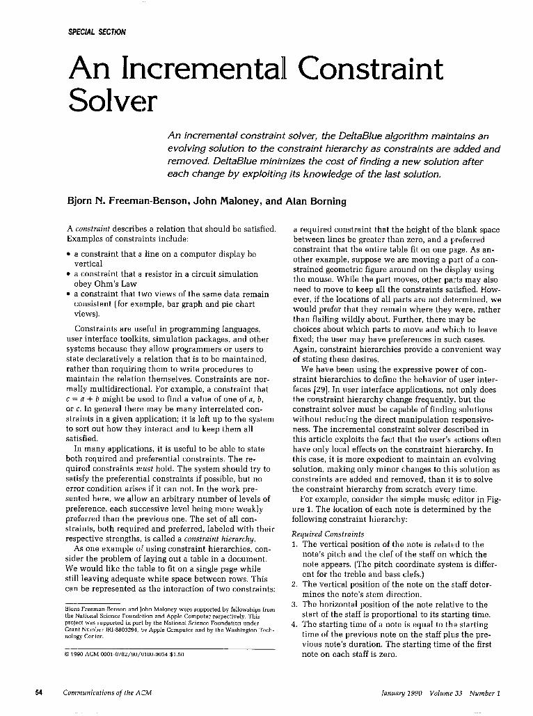
For example, consider the simple music editor in Fig- ure 1. The location of each note is determined by the following constraint hierarchy:

Required Constraints ‘The vertical position of the note is related to the note’s pitch and the clef of the staff on which the note appears. (The pitch coordinate system is different for the treble and bass clefs.) The vertical position of the note on the s;taff determines the note’s stem direction. The horizontal position of the note relative to the start of the staff is proportional to its starting time. The starting time of a note is equal to thee starting time of the previous note on the staff plus the previous note’s duration. The starting time of the first note on each staff is zero.

]anuary 1990 Vohme 3.3 Number I

Special section

Default Constraints 5. A note’s duration, pitch, and position remain the

same (when other parts of the score are edited).

These are the basic layout constraints for a musical score. As the user manipulates the score, constraints are added dynamically in response to dragging notes with the mouse. Two constraints are added for each note being dragged:

Preferred Constraints 6. The horizontal position of the note relative to the

start of the staff is related to the horizontal position of the mouse.

7. The pitch of the note is related to the vertical position of the mouse.

As the notes are dragged, the constraint interpreter alternates calls to the solver to satisfy all satisfiable constraints, and calls to the display update routine. Be- cause constraints 6 and 7 are stronger than constraint 5, the notes will track the mouse, and because constraints 1-4 are required, the score graphics will remain consis-

, i . . . . . . . . . . . . . . . . . . . . . . . . . . . . . . . . . . . . . . . . . . . . . . . . . . . . . . . . . . . . . . . ..-............-............................... I . . . . . . . . . . . i I

FIGURE 1. Music Editor

tent with the music produced. When the mouse button is released, the dynamic constraints are removed and the system is ready for the next user action.

Although the actual layout conventions for musical typesetting are considerably more involved, this example does illustrate how simple constraints can be used to easily determine complex behavior in a user interface.

Related Work Much of the previous and related work on constraint- based languages and systems can be grouped into five areas: geometric layout; simulations; design, analysis, and reasoning support; user interface support; and general-purpose programming languages.

Geometric layout is a natural application for constraints. The earliest work here is Ivan Sutherland’s Sketchpad system [40], developed at MIT in the early 1960s. Sketchpad allowed the user to build up geometric figures using primitive graphical entities and constraints, such as point-on-line, point-on-circle, collinear, and so forth. When possible, constraints were solved using one-pass techniques (first satisfy this constraint, then another, then another, . . . ). When this

technique was not applicable, Sketchpad would resort to an iterative numerical technique, relaxation. Sketch- pad was a pioneering system in interactive graphics and object-oriented programming as well as in constraints. Its requirements for CPU cycles and display bandwidth were such that the full use of its techniques had to await cheaper hardware years later. ThingLab [2, 31 adopted many of the ideas in Sketchpad, and combined them with the extensibility and object-oriented techniques of the Smalltalk programming language [17]. Later versions of ThingLab incorporated such features as constraint hierarchies (as described in this article), incremental compilation, and a graphical facility for defining new kinds of constraints [I, 4, 13, 291. Other constraint-based systems for geometric layout include Juno by Greg Nelson [33], Magritte by James Gosling [18], and IDEAL by Chris Van Wyk [45, 461.

Simulations are another natural application for constraints. For example, in simulating a physics experi- ment, the relevant physical laws can be represented as constraints. In addition to its geometric applications, Sketchpad was used for simulating mechanical link- ages, while ThingLab was used for simulating electrical circuits, highway bridges, and other physical objects. Animus [9] extended ThingLab to include constraints on time, and thus animations. With it, a user could construct simulations of such phenomena as resonance and orbital mechanics. Qualitative physics, an active area of artificial intelligence (AI) research, is concerned with qualitative rather than quantitative analysis and simulation of physical systems [43]. Most such systems employ some sort of constraint mechanism.

Related to simulation systems are ones to help in design and analysis problems. Here, constraints can be used to represent design criteria, properties of devices, and physical laws. Examples of such systems include the circuit analysis system EL by Stallman and Suss- man [37], PRIDE [30], an expert system for designing paper handling systems, and DOC and WORM [34] by Mark Sapossnek. In [39] Sussman and Steele consider the use of constraint networks for representing multiple views on electrical circuits. TK!Solver [24] is a com- mercially available constraint system, with many packages for engineering and financial applications. Levitt [27] uses constraints in a very different design task, namely jazz composition. Finally, there has been con- siderable research in the AI community on solving systems of constraints over finite domains [28]. Two typical applications of such constraint satisfaction problems (CSPs) are scene labeling and map interpretation.

Constraints also provide a way of stating many user interface design requirements, such as maintaining consistency between underlying data and a graphical depiction of that data, maintaining consistency among multiple views, specifying formatting requirements and preferences, and specifying animation events and attri- butes. Both ThingLab and Animus have been used in user-interface applications. Carter and LaLonde [6] use constraints in implementing a syntax-based program editor. Myers’ Peridot system [32] deduces constraints

]anuary 1990 Volume 33 Number 1 Communications of the ACM 55

Special Section

automatically as the user demonstrates the desired ap- pearance and behavior of a user interface; a related system is Coral [4’1], a user-interface toolkit that uses a combination of one-way constraints and active values. Vander Zanden [42] combines constraints and graphics with attribute grammars to produce constraint grammars; his system i:ncludes an incremental constraint satisfier related to the one described in this article. Ege [lo, 111 built a user-interface construction system that used a filter metaphor: source and view objects were related via filters, which were implemented as multi- way constraints. Filters could be composed, both end- to-end and side-by-side, so that more complex interface descriptions could be built from simpler ones. Epstein and LaLonde [12] ‘use constraint hierarchies in control- ling the layout of Smalltalk windows.

Finally, a number of researchers have investigated general-purpose languages that use constraints. Steele’s Ph.D. dissertation [38] is one of the first such efforts; an important characteristic of his system is the mainte- nance of dependency information to support dependency-directed backtracking and to aid in generating explanations. Leler [26] describes Bertrand, a constraint language based on augmented term rewriting. Freeman-Benson [X4] proposes to combine constraints with object-oriented, imperative programming.

Much of the recent research on general-purpose languages with constraints has used logic programming as a base. Jaffar and Lassez [22] describe a scheme CLP(g) for Constraint Logic Programming Languages, which is parameterized by 9, the domain of the constraints. In place of unification, constraints are accumulated and tested for satisfiability over 9, using techniques appropriate to the domain. Several such languages have now been implemented, including Prolog III [7], CLP(W) [19, 231 and CHIP [S, 201. Most of these systems include incremental constraint satisfiers, since constraints are added and deleted dynamically during program execution. CLP(9), for example, includes an incremental version of the Simplex algorithm, while CHIP includes an incremental satisfier for constraints over finite domains. Reference [5] describes a scheme for Hierarchi- cal Constraint Logic Programming languages (HCLP), which integrate CLP(G?) with constraint hierarchies, and reference [44] presents an interpreter for HCLP(9). Saraswat’s Ph.D. dissertation [35] describes a family of concurrent constraint languages, again with roots in logic programming.

Theory A constraint system consists of a set of constraints C and a set of variables V. A constraint is an n-ary relation among a subset of V. Each constraint has a set of methods, any of which may be executed to cause the constraint to be satisfied. Each method uses some of the constraint’s variables as inputs and computes the remainder as outputs. A method may only be executed when all of its inputs and none of its outputs have been determined by other constraints.

The programmer is often willing to relax some constraints if not all of them can be satisfied. To represent this, each constraint in C is labeled with a sttengfh. One of these strengths, the required strength, is special, in that the constraints it labels must be satisfied The re- maining strengths all indicate preferences of varying degrees. There can be an arbitrary number of different strengths. We define Co to be the required constraints in C, C1 to be the most strongly preferred constraints, C, the next weaker level, and so forth, through I,,, where n is the number of distinct non-required strengths.

A solution to a given constraint hierarchy is a map- ping from variables to values. A solution that satisfies all the required constraints in the hierarchy is called admissible. There may be many admissible solutions to a given hierarchy. However, we also want to satisfy the preferred constraints as well as possible, respecting their strengths. Intuitively, the best solutions to the hierarchy are those that satisfy the required constraints, and also satisfy the preferred constra.ints such that no other better solution exists. (There may be several different best solutions.)

To define this set of solutions formally, we use a predicate “better,” called the comparator, that compares two admissible solutions. We first define So, the set of admissible solutions, and then the set S of .best solutions.

So = (x ( Vc E Co x satisfies c)

S = (x J x E So A Vy E S, lbetter(y, x. C))

A number of alternate definitions for comparators are given in [5]. These comparators differ as to .whether they measure constraint satisfaction using an error metric or a simple boolean predicate (satisfied/not satisfied). Orthogonally, they also differ as to whether they compare the admissible solutions by considering one constraint at a time, or whether they take some aggregate measure of how well the constraints are satisfied at a given level. Comparators that compare solutions constraint-by-constraint are local; those that use an aggregate measure are global. Examples of aggregate mea- sures are the weighted sum of the constraint terrors, the weight sum of the squares of the errors, and the maxi- mum of the weighted errors.

The algorithm presented in this article finds solutions based on the locally-predicate-better comparator. This is a local comparator that uses a simple satisfied/not satisfied test. This comparator finds intuitively plausible solutions for a reasonable computational cost. Its definition is:

Solution x is locally-predicate-better than solution y for constraint hierarchy C if there exists s:ome level k such that:

for every constraint c in levels C1 through Ck-*, x satisfies c if and only if y satisfies c,

and, at level Ck, x satisfies every constraint that y does,

and at least one more.

56 Communications of the ACM ]anuary 1990 Volume 33 Number 1

Special Section

By definition, S will not contain any solutions that are worse than some other solution. However, because better is not necessarily a total order, S may contain multiple solutions, none of which is better than the others. The algorithm described here does not enumer- ate multiple solutions; if several equally good solutions exist, it returns only one of them, chosen arbitrarily. Such multiple solutions arise when either the hierarchy allows some degrees of freedom (the under- constrained case), or when there is a conflict between preferred constraints of the same strength, forcing the constraint solver to choose among them (the over- constrained case). Reference [IS] discusses these issues in more depth and provides an algorithm for enumerat- ing both types of multiple solutions. Similarly, the interpreter for the Hierarchical Constraint Logic Program- ming language [5] produces alternate solutions upon backtracking.

Constraint Solvers Although constraints are a convenient mechanism for specifying relations among objects, their power leads to a weakness-one can use constraints to specify problems that are very difficult to solve. This motivates the development of increasingly powerful constraint- solving algorithms. Unfortunately, as the generality of these algorithms increases, so does their run time. Thus, to solve a variety of constraints both efficiently and correctly, a broad range of algorithms is necessary. For some systems, such as those we use in our user- interface research, a fast, restricted algorithm is desir- able. For other systems, such as general engineering problem solvers, a slower but more complete algorithm is required.

Furthermore, although the ideal algorithm would be tailorable with one of the comparators discussed in [5], the hard reality is that each algorithm is designed around only a few comparators. Again the slower, more general, algorithms will be more complete and solve for more of the comparators, whereas the faster, more specific, algorithms will be limited to a single comparator.

As a result, we have designed a “Spectrum of Algo- rithms” for solving constraint hierarchies, each at a different point in the engineering trade-off of generality versus efficiency:

Red: The Red algorithm uses a generalized graph rewriting system based on Bertrand [2S] and is capable of solving hierarchies with cycles and simultaneous equations. It is more general and slower than most of the other algorithms.

Orange: The Orange algorithm is based on the Simplex algorithm for solving linear programming problems, [31], and is specialized for finding one or all solutions to hierarchies of linear equality and inequality constraints.

Yellow: The Yellow algorithm uses classical relaxation, an iterative hill-climbing technique [40], to produce a least-squares-better solution. It is slower than Orange, but it can handle non-linear equations.

Green: The Green algorithm solves constraints over finite domains (such as the ten digits zero to nine, or the three traffic light colors) with a combination of local propagation and generate-and-test tree search.

Blue: Blue is a fast local propagation algorithm [2, 18, 391, customized for the locally-predicate-better comparator. However, it cannot solve constraint hierarchies involving cycles.

DeltaBlue: DeltaBlue is an incremental version of the Blue algorithm.

We have implemented Orange, Yellow, Green, Blue, and of course, DeltaBlue.

THE DELTABLUE ALGORITHM In interactive applications, the constraint hierarchy often evolves gradually, a fact that can be exploited by an incremental constraint satisfier. An incremental constraint satisfier maintains an evolving “current solution” to the constraints. As constraints are added to and removed from the constraint hierarchy, the incremental satisfier modifies this current solution to find a solution that satisfies the new constraint hierarchy.

The DeltaBlue algorithm is an incremental version of the Blue algorithm. In Blue and DeltaBlue, each constraint has a set of methods that can be invoked to satisfy the constraint. For example,

c=u+b

has three methods:

ctu+b btc-a utc-b

Therefore, the task of the DeltaBlue is to decide which constraints should be satisfied, which method should be used to satisfy each constraint, and in what order those methods should be invoked.

In the remainder of this section, we present a high- level description of the DeltaBlue algorithm and illustrate its behavior through several examples. A more precise pseudo-code description of the algorithm may be found in the appendix of [16].

Prelude The DeltaBlue algorithm uses three categories of data: the constraints in the hierarchy C, the constrained variables V, and the current solution P. P, also known as a plan, is a directed acyclic dataflow graph distributed throughout the constraint and variable objects: each variable knows which constraint determines its value, while each constraint knows if it is currently satisfied and, if so, which method it uses.

The initial configuration is C = 0 and V = 0 (i.e., no constraints and no variables). The client program interfaces with the DeltaBlue solver through four entry points:

add-constraint add-variable

remove-constraint remove-variable

Variables must be added to the graph before constraints using them can be defined. Removing a variable re-

January 1990 Volume 33 Number 1 Communications of the ACM 57

Special Section

moves any extant constraints on that variable as well. The current solution P is incrementally updated after each add-constraint and remove-constraint operation.

The DeltaBlue algorithm cannot solve under-constrained hierarchies, so an invisible very weak stay constraint is attached to each variable as it is added. A stay constraint constrains the value of the variable to remain unchanged. Because this system-supplied stay constraint is weaker than any constraint the client program may add, it will only be used if the variable is not otherwise constrained, i.e., if the variable is undercon- strained.

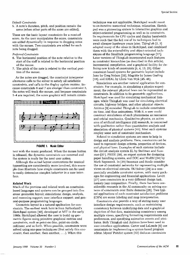
Walkabout Strength The key idea behind DeltaBlue is to associate sufficient information with each variable to allow the algorithm to predict the effect of adding a given constraint by examining only the immediate operands of that constraint. This information is called the walkabout strength of the variable (the name comes from the Australian custom of a long walk to clear the mind), defined as follows:

Variable ZI is determined by method m of constraint c. n’s walkabout strength is the minimum of c’s strength and the walkabout strengths of m’s inputs.

One can think of the walkabout strength as the strength of the weakest “upstream” constraint, i.e., the weakest ancestor constraint (in the current solution P) that can be reached via a reversible sequence of constraints. Thus the walkabout strength represents the strength of the weakest constraint that could be revoked to allow another constraint to be satisfied.

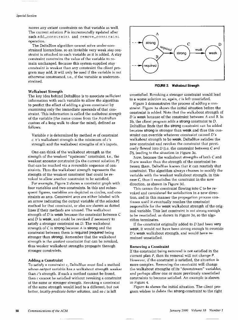
For example, Figure 2 shows a constraint graph with four variables and two constraints. In this and subse- quent figures, variables are depicted as circles, and constraints as arcs. Constraint arcs are either labeled with an arrow indicating the output variable of the selected method for that constraint, or else are shown as dotted lines if their methods are unused. The walkabout strength of D is weak because the constraint between C and D is weak, and could be revoked if necessary to satisfy a stronger constraint on D. The walkabout strength of C is strong because A is strong and the constraint between them is required (required being stronger than strong). Remember that the walkabout strength is the weakest constraint that can be revoked, thus weaker walkabout strengths propagate through stronger constraints.

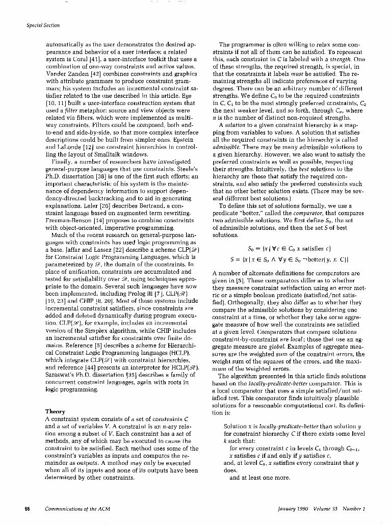
Adding a Constraint To satisfy a constraint c, DeltaBlue must find a method whose output variable has a walkabout strength weaker than c’s strength. If such a method cannot be found, then c cannot be satisfied without revoking a constraint of the same or stronger strength. Revoking a constraint of the same strength would lead to a different, but not better, locally-predicate-better solution, and so c is left

58 Communications of th: ACM

FIGURE 2. Walkabout Strength

unsatisfied. Revoking a stronger constraint would lead to a worse solution so, again, c is left unsatisfi.ed.

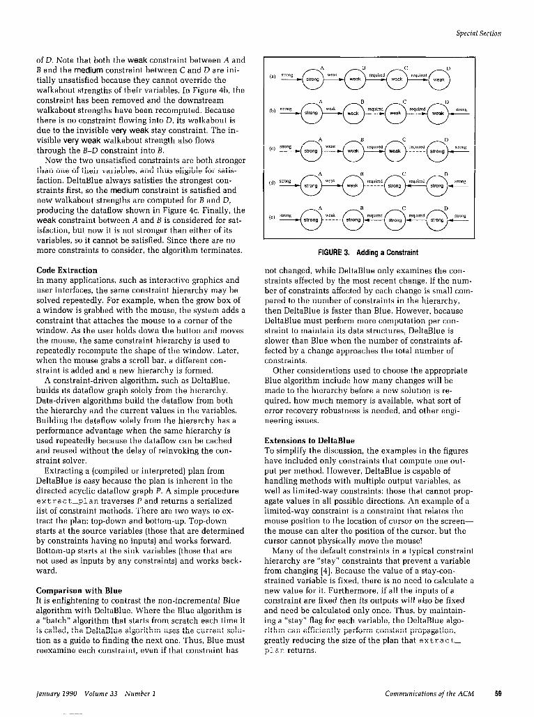
Figure 3 demonstrates the process of adding a constraint. Figure 3a shows the initial situation before the constraint is added. Note that the walkabout strength of D is weak because of the constraint between .A and B. In 3b, the client program adds a strong constraint to D. DeltaBlue finds that the strong constraint car. be added because strong is stronger than weak and thus this constraint can override whatever constraint caused D’s walkabout strength to be weak. DeltaBlue satisfies the new constraint and revokes the constraint th.st previously flowed into D (i.e. the constraint between C and D), leading to the situation in Figure 3c.

Now, because the walkabout strengths of both C and D are weaker than the strength of the constraint between them, DeltaBlue knows that it can resatisfy that constraint. The algorithm always chooses to modify the variable with the weakest walkabout strength, in this case C, thus it resatisfies the constraint in the new direction, as shown in Figure 3d.

This causes the constraint flowing into C to be revoked and considered for satisfaction in a new direction, and in this manner the propagation process continues until it eventually reaches the constraint responsible for the weak walkabout strength of the original variable. This last constraint is not strong enough to be resatisfied, as shown in Figure 3e, so the algorithm terminates.

If the constraint originally added to D had been very weak, it would not have been strong enough to override D’s weak walkabout strength, and would have re- mained unsatisfied.

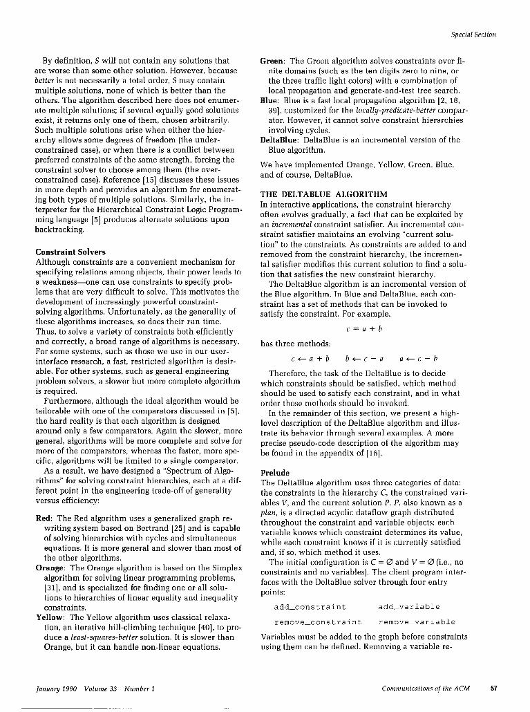
Removing a Constraint If the constraint being removed is not satisfied in the current plan P, then its removal will not change P. However, if the constraint is satisfied, the situation is more complex. Removing the constraint will change the walkabout strengths of its “downstream” variables, and perhaps allow one or more previously unsatisfied constraints to become satisfied. An example is shown in Figure 4.

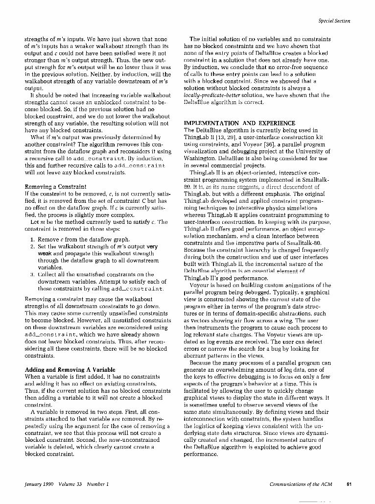
Figure 4a shows the initial situation. The client program wishes to delete the strong constraint to the right

]anua y 1990 Volume 33 Number 1

Special Section

of D. Note that both the weak constraint between A and B and the medium constraint between C and D are ini- tially unsatisfied because they cannot override the walkabout strengths of their variables. In Figure 4b, the constraint has been removed and the downstream walkabout strengths have been recomputed. Because there is no constraint flowing into D, its walkabout is due to the invisible very weak stay constraint. The invisible very weak walkabout strength also flows through the B-D constraint into B.

Now the two unsatisfied constraints are both stronger than one of their variables, and thus eligible for satisfaction. DeltaBlue always satisfies the strongest constraints first, so the medium constraint is satisfied and new walkabout strengths are computed for B and D, producing the dataflow shown in Figure 4c. Finally, the weak constraint between A and B is considered for satisfaction, but now it is not stronger than either of its variables, so it cannot be satisfied. Since there are no more constraints to consider, the algorithm terminates.

Code Extraction In many applications, such as interactive graphics and user interfaces, the same constraint hierarchy may be solved repeatedly. For example, when the grow box of a window is grabbed with the mouse, the system adds a constraint that attaches the mouse to a corner of the window. As the user holds down the button and moves the mouse, the same constraint hierarchy is used to repeatedly recompute the shape of the window. Later, when the mouse grabs a scroll bar, a different constraint is added and a new hierarchy is formed.

A constraint-driven algorithm, such as DeltaBlue, builds its dataflow graph solely from the hierarchy. Data-driven algorithms build the dataflow from both the hierarchy and the current values in the variables. Building the dataflow solely from the hierarchy has a performance advantage when the same hierarchy is used repeatedly because the dataflow can be cached and reused without the delay of reinvoking the constraint solver.

Extracting a (compiled or interpreted) plan from DeltaBlue is easy because the plan is inherent in the directed acyclic dataflow graph P. A simple procedure extract-plan traverses P and returns a serialized list of constraint methods. There are two ways to extract the plan: top-down and bottom-up. Top-down starts at the source variables (those that are determined by constraints having no inputs) and works forward. Bottom-up starts at the sink variables (those that are not used as inputs by any constraints) and works back- ward.

Comparison with Blue It is enlightening to contrast the non-incremental Blue algorithm with DeltaBlue. Where the Blue algorithm is a “batch” algorithm that starts from scratch each time it is called, the DeltaBlue algorithm uses the current solution as a guide to finding the next one. Thus, Blue must reexamine each constraint, even if that constraint has

FIGURE 3. Adding a Constraint

not changed, while DeltaBlue only examines the constraints affected by the most recent change. If the number of constraints affected by each change is small com- pared to the number of constraints in the hierarchy, then DeltaBlue is faster than Blue. However, because DeltaBlue must perform more computation per constraint to maintain its data structures, DeltaBlue is slower than Blue when the number of constraints affected by a change approaches the total number of constraints.

Other considerations used to choose the appropriate Blue algorithm include how many changes will be made to the hierarchy before a new solution is required, how much memory is available, what sort of error recovery robustness is needed, and other engineering issues.

Extensions to DeltaBlue To simplify the discussion, the examples in the figures have included only constraints that compute one output per method. However, DeltaBlue is capable of handling methods with multiple output variables, as well as limited-way constraints: those that cannot propagate values in all possible directions. An example of a limited-way constraint is a constraint that relates the mouse position to the location of cursor on the screen- the mouse can alter the position of the cursor, but the cursor cannot physically move the mouse!

Many of the default constraints in a typical constraint hierarchy are “stay” constraints that prevent a variable from changing [a]. Because the value of a stay-constrained variable is fixed, there is no need to calculate a new value for it. Furthermore, if all the inputs of a constraint are fixed then its outputs will also be fixed and need be calculated only once. Thus, by maintaining a “stay” flag for each variable, the DeltaBlue algorithm can efficiently perform constant propagation, greatly reducing the size of the plan that extract- plan returns.

]anuay 1990 Volume 33 Number 1 Communications of the ACM 59

Special Section

FIGURE 4. Removing a Constraint

The basic DeltaBlue algorithm can only solve wzique constraints-those that determine unique values for their outputs given values for their inputs. A non- unique constraint such as “x > 5” restricts but does not uniquely fix the value of x. DeltaBlue has been extended to solve non-unique constraints, but a full discussion of the revised algorithm is beyond the scope of this article.

CORRECTNESS PROOF We will show that any solution generated by the DeltaBlue algorithm is a locally-predicate-better solution to the current constraint hierarchy. If there is a cycle, or if there are conflicting required constraints, the algorithm will report this fact and halt without generating any solution.

We first define the notion of a blocked constraint and present a lemma that says that if there are no blocked constraints in a solution, then that solution is a locally- predicate-better solution. We then show that if the current solution has no blocked constraints, then neither will the solution resulting from a successful call to any of the four entry points of the algorithm (add-con straint,add-variable,remove_constraint, and remove-variable). By induction, then, we will have demonstrated the correctness of the algorithm.

The Blocked Constraint Lemma Definition. A blocked constraint is an unsatisfied constraint whose strength is stronger than the walkabout strength of one of its potential output variables.

Lemma. If there are no blocked constraints, then the set of satisfied constraints represents a locully-predicate- better solution to the constraint hierarchy.

60 Communications of the ACM Ianuary 2990 Volume 33 Number 2

Proof. Given a solution & produced by DeltaBlue, as- sume for the sake of contradiction that there is a solution W better than solution &. Th.en, by the definition of locally-predicate-better, there is some level k in the hierarchy such that &’ satisfies every constraint that & does through level k, and at least one additional constraint c at level k. Let D, be the variable of the constraint c with the weakest walkabout strength, and let z)= have a walkabout strength of ZU$ in @. Now, because c is unsatisfied in M and ~7 has no blocked constraints, c is not stronger than w:~. However, because c is satisfied in 9, c must be stronger than wg. This is a c:ontradic- tion, so there must not be any solution bette:r than @.

Adding a Constraint DeltaBlue adds a constraint c in four stages:

1. Choose a method m such that the walkabout strength of m’s output is no stronger tha.n the walkabout strength of the output of any of c’s other methods. (a) If no such method can be found, c is left unsatis-

fied. If c is a required constraint, halt with an error indicating a conflict between required constraints (an over-constrained problem).

(b) If adding the selected method m would create a cycle in the dataflow graph of the solution, halt with an error indicating that a cycle has been encountered (cycles are not handled by Delta- Blue).

2. Insert c in the current solution using method m. 3. Compute the walkabout strength of m’s output ac-

cording to the definition of walkabout strength, and propagate this walkabout strength through the dataflow graph to al1 downstream variables.

4. If m’s output was previously determined by a constraint d, d is removed from the dataflow graph and reconsidered with a recursive call to <add- constraint.

Observe that the process of adding a constraint may result in one of several errors. In this case, the algorithm halts without producing a solution; it does not, however, produce an incorrect solution.

If no method for satisfying c can be found in step one, it is because c is not stronger than any of its possible outputs. By definition, c is not a blocked constraint.

If a method is found in step one [and the method does not produce a cycle), the constraint is satisfied. A satisfied constraint is not a blocked constraint. However, satisfying c changes the walkabout strength of the output of m and all downstream variables. We must show that this will not cause a constraint to become blocked.

First, observe that the walkabout strength of m’s output cannot go down by adding c. This is bec:ause we chose a method whose output had the minimum walkabout strength, so all inputs to m must have an equal or stronger walkabout strength than m’s output has. By the definition, the new walkabout strength for m’s output is the minimum of c’s strength and the walkabout

strengths of m’s inputs. We have just shown that none of m’s inputs has a weaker walkabout strength than its output and c could not have been satisfied were it not stronger than m’s output strength. Thus, the new output strength for m’s output will be no lower than it was in the previous solution. Neither, by induction, will the walkabout strength of any variable downstream of m’s output.

It should be noted that increasing variable walkabout strengths cannot cause an unblocked constraint to become blocked. So, if the previous solution had no blocked constraint, and we do not lower the walkabout strength of any variable, the resulting solution will not have any blocked constraints.

What if m’s output was previously determined by another constraint? The algorithm removes this constraint from the dataflow graph and reconsiders it using a recursive call to add-constraint. By induction, this and further recursive calls to add-constraint will not leave any blocked constraints.

Removing a Constraint If the constraint to be removed, c, is not currently satisfied, it is removed from the set of constraint C but has no effect on the dataflow graph. If c is currently satisfied, the process is slightly more complex.

Let m be the method currently used to satisfy c. The constraint is removed in three steps:

Remove c from the dataflow graph. Set the walkabout strength of m’s output very weak and propagate this walkabout strength through the dataflow graph to all downstream variables. Collect all the unsatisfied constraints on the downstream variables. Attempt to satisfy each of these constraints by calling add-constraint.

Removing a constraint may cause the walkabout strengths of all downstream constraints to go down. This may cause some currently unsatisfied constraints to become blocked. However, all unsatisfied constraints on these downstream variables are reconsidered using add-constraint, which we have already shown does not leave blocked constraints. Thus, after recon- sidering all these constraints, there will be no blocked constraints.

Adding and Removing A Variable When a variable is first added, it has no constraints and adding it has no effect on existing constraints. Thus, if the current solution has no blocked constraints then adding a variable to it will not create a blocked constraint.

A variable is removed in two steps. First, all constraints attached to that variable are removed. By repeatedly using the argument for the case of removing a constraint, we see that this process will not create a blocked constraint. Second, the now-unconstrained variable is deleted, which clearly cannot create a blocked constraint.

Special Section

The initial solution of no variables and no constraints has no blocked constraints and we have shown that none of the entry points of DeltaBlue creates a blocked constraint in a solution that does not already have one. By induction, we conclude that no error-free sequence of calls to these entry points can lead to a solution with a blocked constraint. Since we showed that a solution without blocked constraints is always a locally-predicate-better solution, we have shown that the DeltaBlue algorithm is correct.

IMPLEMENTATION AND EXPERIENCE The DeltaBlue algorithm is currently being used in ThingLab II [13, 281, a user-interface construction kit using constraints, and Voyeur 1361, a parallel program visualization and debugging project at the University of Washington. DeltaBlue is also being considered for use in several commercial projects.

ThingLab II is an object-oriented, interactive constraint programming system implemented in Smalltalk- 80. It is, as its name suggests, a direct descendent of ThingLab, but with a different emphasis. The original ThingLab developed and applied constraint programming techniques to interactive physics simulations whereas ThingLab II applies constraint programming to user-interface construction. In keeping with its purpose, ThingLab II offers good performance, an object encap- sulation mechanism, and a clean interface between constraints and the imperative parts of Smalltalk-80. Because the constraint hierarchy is changed frequently during both the construction and use of user interfaces built with ThingLab II, the incremental nature of the DeltaBlue algorithm is an essential element of ThingLab II’s good performance.

Voyeur is based on building custom animations of the parallel program being debugged. Typically, a graphical view is constructed showing the current state of the program either in terms of the program’s data structures or in terms of domain-specific abstractions, such as vectors showing air flow across a wing. The user then instruments the program to cause each process to log relevant state changes. The Voyeur views are updated as log events are received. The user can detect errors or narrow the search for a bug by looking for aberrant patterns in the views.

Because the many processes of a parallel program can generate an overwhelming amount of log data, one of the keys to effective debugging is to focus on only a few aspects of the program’s behavior at a time. This is facilitated by allowing the user to quickly change graphical views to display the state in different ways. It is sometimes useful to observe several views of the same state simultaneously. By defining views and their interconnection with constraints, the system handles the logistics of keeping views consistent with the underlying state data structures. Since views are dynamically created and changed, the incremental nature of the DeltaBlue algorithm is exploited to achieve good performance.

Ianuary 2990 Volume 33 Number 1 Communications of the ACM 61

Special Section

Compilation Although Blue and DeltaBlue are efficient enough to solve dozens of constraints in seconds, they can be applied to even larger constraint problems while maintaining good performance by using a module compilation mechanism. We have developed such a mechanism [13] to allow large user interfaces to be built with ThingLab II.

In ThingLab II, the user-manipulable entities are col- lections of objects known as Things. ThingLab II provides a large number of primitive Things equivalent to their basic operations and data structures of any other high-level language: numerical operations, points, strings, bitmaps, conversions, etc. Using a construction kit metaphor, new Things can be built out of primitive Things. These constructed Things can be used as the component parts of higher-level Things, which can in turn be used to build still higher-level Things.

At any point in this construction process, a Thing may be compiled to create a Module. A module retains the external behavior of the Thing it came from and may be used as a building block like any other Thing, but its internal implementation is more efficient in both storage space and execution speed. Since its internal details are hidde-n, a module also provides abstrac- tion and information hiding similar to that provided by an Ada package, or a C++ or Smalltalk class. Modules are appropriate in applications where the behavior of the Thing will not change, efficiency is an issue, or the implementation is proprietary. An uncompiled Thing is a better choice in applications where the internal struc- ture of the Thing must be visible or when the system is under rapid development. In other words, Modules and Things represent the two sides of the classical tradeoff between compilation and interpretation.

The module compiler replaces the internal variables and constraints of a Thing with a set of compiled procedures, or module methods, ea:h of which encapsulates one solution to the original constraints. In addition to the module methods, the module compiler constructs procedures that aid in selecting an appropriate module method for a given set of external constraints and procedures that efficiently propagate DeltaBlue walkabout strengths through the module. These procedures are the result of partially evaluating the DeltaBlue algorithm over the original constraints. For a more complete discussion of the module compiler, the reader is referred to [13].

Modules in ThingLab II were inspired by the compo- nents of Arie1 and Fabrik [Zl], and by the Object Defi- ner [l] from the original ThingLab. These systems, however, could not produce objects for use outside their development environment whereas a simple mod- ification to ThingLab II allows modules to be used as objects outside of ThingLab II.

CONCLUSION The DeltaBlue algorithm has achieved its goal of being a fast algorithm for satisfying dynamically changing constraint hierarchies (see [29] for performance fig-

ures). Our research group at the [Jniversity of Washing- ton continues to explore other constraint hie;:archy algorithms, and especially other incremental constraint hierarchy algorithms. The DeltaBlue algorithm was created by a careful study of the data structures and behavior of the Blue algorithm. We hope that similar study should produce DeltaRed and DeltaOrange algorithms as well.

Acknowledgments. Thanks to Jed Harris for his com- ments on an earlier draft of this article.

REFERENCES 1. Borning. A. Graphically defining new building blocks in ThingLab.

Human-Comput. Interact. 2, 4 (Apr. 19861, 269-295. 2. Borning, A.H. The programming language aspects of ThingLab. a

constraint-oriented simulation laboratory. ACM Trans. Prog. Lang. spt. 3. (Oct. igal), 353-387.

3. Borning, A. H. ThingLab-A Constraint-Orienfed Simufalion Laboratory. Ph.D. dissertation. Computer Science Department, Stanford, March 1979. A revised version is published as Xerox Palo Also Research Center Rep. SSL-79-3 (July 1979).

4. Borning. A., Duisberg, R., Freeman-Benson, B., Kramer, A., and Woolf, M. Constraint hierarchies. In Proceedings of the 1987 ACM Conference on Object-Oriented Programming Systems, L.arlguages and Applications (Orlando, Fla., October 4-a, 1987), pp. 48-60.

8. Borning, A., Maher, M.. Martindale, A., and Wilson, M. Constraint hierarchies and logic programming. In Proceedings of the Sixth Znter- national Logic Programming Conference, (Lisbon, Portugel, June 1989). pp. 149-164. Also published as Tech. Rep. 88-11-10, Computer Sci- ence Department, University of Washington, November 1988.

6. Carter, C.A., and LaLonde, W.R. The design of a program editor based on constraints. Tech. Rep. CS TR 50, Carleton University, May 1984.

7. Colmerauer. A. An introduction to Proloa III. Draft. Grouue Intelli-

8.

9.

10.

11.

12.

13.

14.

15.

16.

17.

18.

19.

20.

gence Artificielle. Universite Aix-Marseille II, November*l987. Dincbas, M.. Van Hentenryck, P., Simonis, H.. Aggoun A.. Graf, T.. and Bertheir, F. The constraint logic programming language CHIP. In Proceedings of International Conference on Fifth Generation Computer Systems, FGCS-88 (Tokyo, Japan. 1988). Duisberg. R. Constraint-based animation: The implementation of temporal constraints in the animus system. Ph.D. dissertation, Uni- versity of Washington, 1986. Published as U.W. Computer Science Department Tech. Rep. No. 86-09-01. Ege, R. K. Automatic Generation of Interactive Display:: LIsing Con- straints. Ph.D. dissertation, Department of Computer Science and Engineering, Oregon Graduate Center. August 1987. Ege, R., Maier, D., and Borning, A. The filter browser--Defining interfaces graphically. In Proceedings of the European Conference on Object-Oriented Programming (Paris, June 1987), pp. 155-165. Epstein, D., and LaLonde. W. A smalltalk window system based on constraints. In Proceedings of the 1988 ACM Conference VR Object- Oriented Programming Systems, Languages and Applications [San Diego, Sept. 1988), pp. 83-94. Freeman-Benson, B. A module mechanism for constraints in Small- talk. In Proceedings of the 1989 ACM Conference on Object-Oriented Programming Systems, Languages and Applications (New Orleans, Oct. 1989), 389-396. Also published as Tech. Rep. 89-05-03. Com- puter Science Dept., University of Washington, May 1!)89. Freeman-Benson. B. Constraint Imperative Programming: A Re- search Proposal. Tech. Rep. 89-04-06, Computer Scienx Dept., Uni- versity of Washington, 1989. Freeman-Benson, B.N. Multiple solutions from constraint hierarchies. Tech. Rep. 88-04-02, University of Washington, April 1988. Freeman-Benson, B., Maloney, J,, and Borning, A. The DeltaBlue algorithm: An incremental constraint hierarchy solver. Tech. Rep. 89-08-06, Depart. of Computer Science and Engineering, University of Washington, August 1989. Goldberg, A., and Robson, D. Smalltalk-80: The Language and Its Im- plementation. Addison-Wesley, Reading, Mass., 1983. Gosling, J. Algebraic Constraints. Ph.D. dissertation, Carnegie-MeI- lon University, May 1983. Published as CMU Computer Science Department Tech. Rep. CMU-CS-83-132. Heintze, N.. Jaffar, J., Michaylov. S., Stuckey, P., and Yap, R. The CLP(%] programmer’s manual. Tech. Rep., Computer Science Dept., Monash University, 1987. van Hentenryck, P. Constraint Satisfaction in Logic Programming. MIT Press, Cambridge, Mass., 1989.

62 Communications of the ACM January 1990 Volume 33 Number 1

Documents

An Incremental Constraint Solver - Georgia Institute of … Incremental Constraint Solver An incremental constraint solver, the DeltaBlue algorithm maintains an evolving solution to