Embed Size (px)
Citation preview

DOT HS 811 109 March 2009
An In-Service Analysis of Maintenance And Repair Expenses for the Anti-Lock Brake System and Underride Guard for Tractors and Trailers
This report is free of charge from the NHTSA Web site at wwwnhtsadotgov
DISCLAIMER
This publication is distributed by the US Department of Transportation National Highway Traffic Safety Administration in the interest of information exchange The opinions findings and conclusions expressed in this publication are those of the author and not necessarily those of the Department of Transportation or the National Highway Traffic Safety Administration The United States Government assumes no liability for its contents or use thereof If trade names manufacturersrsquo names or specific products are mentioned it is because they are considered essential to the object of the publication and should not be construed as an endorsement The United States Government does not endorse products or manufacturers
Technical Report Documentation Page
1 Report No
DOT HS 811 109
2 Government Accession No 3 Recipientrsquos Catalog No
4 Title and Subtitle
An In-Service Analysis of Maintenance and Repair Expenses for the Anti-Lock Brake System and Underride Guard for Tractors and Trailers
5 Report Date
March 2009 6 Performing Organization Code
7 Author(s)
Kirk Allen PhD
8 Performing Organization Report No
9 Performing Organization Name and Address
Evaluation Division National Center for Statistics and Analysis National Highway Traffic Safety Administration Washington DC 20590
10 Work Unit No (TRAIS)
11 Contract or Grant No
12 Sponsoring Agency Name and Address
National Highway Traffic Safety Administration 1200 New Jersey Avenue SE Washington DC 20590
13 Type of Report and Period Covered
NHTSA Technical Report 14 Sponsoring Agency Code
15 Supplementary Notes
16 Abstract
Federal Motor Vehicle Safety Standards (FMVSS) Nos 121 and 105 mandate antilock braking systems (ABS) on all air-braked vehicles and hydraulic-braked trucks and buses with a gross vehicle weight rating (GVWR) of 10000 pounds or greater The primary purpose of this report is to analyze the maintenance and repair expenses to the ABS systems of tractors and trailers A contractor assembled a database with a census of repair receipts from 13 trucking fleets during the period of about 2000 to 2003 with over 4000 vehicles total
bull The average ABS expenses per month of operation were $085 for tractors and $025 for trailers (in 2007 dollars) for vehicles classified built after the effective date for ABS implementation
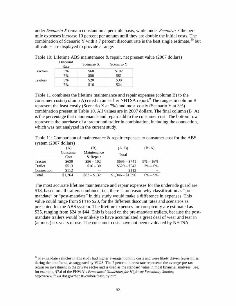
bull Across a vehicle lifetime the net present value of the maintenance and repair expenses is estimated to range from $56 to $102 for tractors and from $16 to $30 for trailers These values are relatively small compared to the cost of equipping new vehicles with ABS systems estimated as $639 for tractors and $513 for trailers in an earlier NHTSA report
bull The presence of the ABS system does not appear to increase overall maintenance expenses to the brake system Older vehicles manufactured before the effective date for ABS implementation had higher brake expenses both per month of service and as a percentage of total maintenance expenses during the survey
bull The average maintenance and repair expenses to the underride guards mandated on trailers with a GVWR of 10000 pounds or greater by FMVSS Nos 223 and 224 were $016 per month of service representing a net present value of $15 over the vehiclersquos lifetime
17 Key Words
anti-lock braking system (ABS) underride guard (URG) in-service tractors trailers statistical analysis FMVSS maintenance repair
18 Distribution Statement
This report is free of charge from the NHTSA Web site at wwwnhtsadotgov
19 Security Classif (Of this report)
Unclassified 20 Security Classif (Of this page)
Unclassified 21 No of Pages
76 22 Price
Form DOT F 17007 (8-72) Reproduction of completed page authorized
An In-Service Analysis of Maintenance and Repair Expenses for the Anti-Lock Brake System and Underride Guard for Tractors and Trailers
Summary 1 List of Figures 3 List of Tables 4 Background5
Scope of current project 5 Earlier work 5
Methodology8 Data characteristics 8 Database structure10 Misclassifications of brake and ABS repairs 13 Database improvements 14
Examples of reclassified orders 14 Calculation of brake repair costs17 Calculation of underride guard repair costs 18 Calculation of conspicuity tape repair costs 19 Other adjustments and corrections20
Vehicle exposure20 Invalidity of miles 21 Exposure using months 22 Evidence that orders are time-sequential 25 Adjustments to months 28 Cost inflation method41
Results47 Expenses per month of exposure 47 Lifetime expenses 52 Fleet differences54 Inferential analysis of cost differences 60
Appendix A VMRS Codes 65 A1 Vehicle systems65 A2 Brake components66 A3 ABS assemblies67
Appendix B Probability of Survival 68
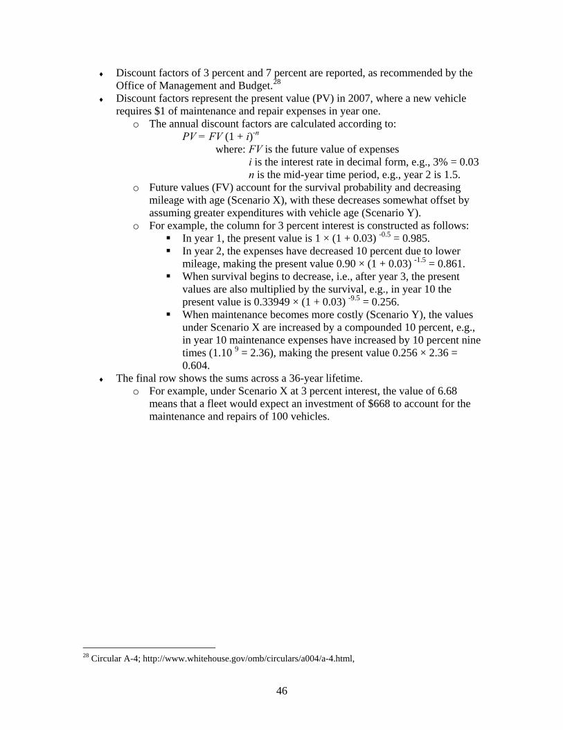
Summary
Federal Motor Vehicle Safety Standards (FMVSS) numbers 121 and 105 mandate antilock braking systems (ABS) on all air-braked vehicles and hydraulic-braked trucks and buses with gross vehicle weight ratings (GVWRs) of 10000 pounds or greater Standards number 223 and 224 mandate strength-tested underride guards (URGs) on trailers with GVWRs of 10000 pounds or greater NHTSA evaluates the cost of its regulations to the consumer including the initial cost of adding safety technology or systems to new vehicles and the lifetime cost of maintaining and repairing the systems
For a study of the maintenance and repair costs of ABS and URG NHTSA contractors assembled a database consisting of repair-line details for over 4000 in-service vehicles from 13 trucking fleets that perform in-house maintenance In general repairs were tracked during 1998-2003 NHTSA contractors and staff prepared the database for analysis by identifying repairs involving ABS components the brake system generally or URG and ascertaining for how many months each vehiclersquos repairs were tracked That made it possible to estimate maintenance and repair costs per month Costs were estimated for tractors and semi-trailers single-unit-trucks were originally part of the study but the fleets did not operate enough of them for meaningful cost estimates
The principal finding is that the repair and maintenance costs for the ABS system averaged $085 per month on tractors and $025 per month on trailers in 2007 dollars Over the lifetime of the vehicles given a 7-percent discount rate and assuming costs per mile increase by 10 percent a year as a vehicle ages (up to year nine) that amounts to a net present value in 2007 dollars of $81 per tractor and $24 per trailer The net present value could be lower if maintenance expenses remain constant on a per-mile basis ($56 for tractors $16 for trailers) or higher if the expense stream is discounted at only 3 percent ($102 for tractors $30 for trailers) The derivation of these estimates is presented in sufficient detail that the interested reader could modify the parameters to suit his needs The lifetime maintenance costs are substantially smaller than the initial costs of equipping tractors and trailers with ABS $639 and $513 respectively reported in earlier NHTSA studies
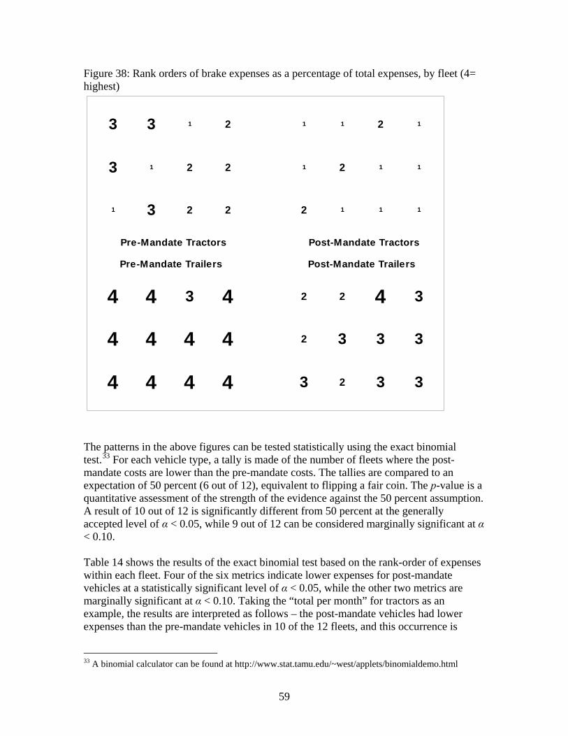
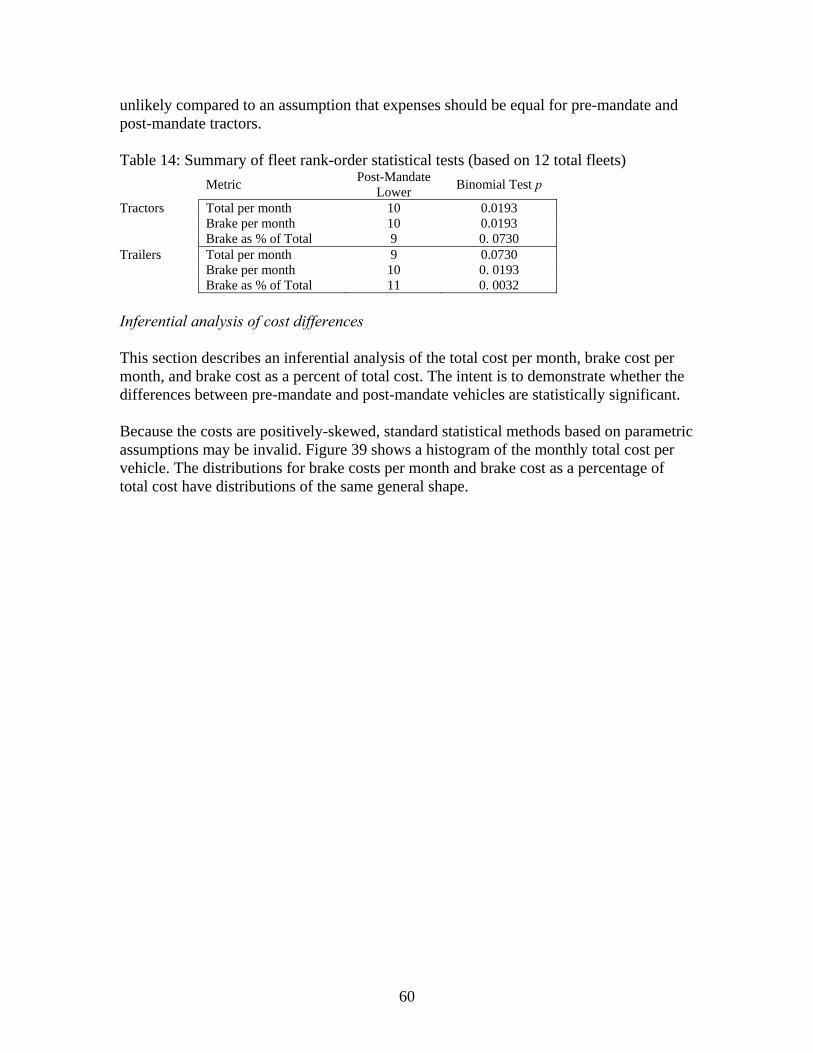
A second study objective was to determine if the addition of ABS increased the cost of maintaining and repairing the brake system as a whole The results indicate that the presence of the ABS system did not increase maintenance and repair expenses to the brake system either in terms of dollars per month of service or brake expenses as a percentage of total vehicle expenses In fact the monthly total and brake expenses as well as brake expenses as a percentage of total repair and maintenance expenses were shown to be significantly lower for post-Standard 121 vehicles for both tractors and trailers based on a statistical test which controlled for fleet-to-fleet differences
Two caveats are necessary for applying the ABS results of this report First though the contractor attempted to select fleets representing a range of operating characteristics it remains a convenience sample rather than one based on probabilistic sampling The results may not therefore apply to the population of all trucking fleets Second most
1
vehicles were tracked for a period of less than three years Post-mandate vehicles could have been at most 6 years old by the end of the survey If the ABS system begins to break down more frequently at later dates this could not have been captured
The cost of replacing repairing or maintaining URG on trailers averaged $016 per month a net present value of $15 over the life of a trailer Expenses were analyzed separately for conspicuity tape a small portion of which is placed on the URG but in minimal length compared to the rest of the trailer The best estimate for the application of conspicuity tape is $037 per month representing $35 over a trailerrsquos lifetime As with ABS expenses the caveat is that very few trailers in the database incurred expenses for URG and conspicuity tape It may take additional years to accumulate sufficient wear and tear to merit replacement There is no indication that a large number of URG replacements occurred due to crash involvement
2
List of Figures
Figure 1 Database components 11 Figure 2 Sample order 12 Figure 3 Illustration of database correction 13Figure 4 Example of actual data entire order counted towards ABS 14 Figure 5 Reclassified order ABS sensor repair 15 Figure 6 Reclassified order ECU with labor uncertain 15Figure 7 Reclassified order ABS light stays on 16 Figure 8 Reclassified order ABS light not functioning 16 Figure 9 Reclassified order sensor repair with small extra parts 17 Figure 10 Order with URG replacement 18 Figure 11 Order with other URG repair 19 Figure 12 Order with other conspicuity tape replacement labor uncertain 19 Figure 13 Order with other conspicuity tape replacement labor identifiable 20 Figure 14 Enhanced boxplot of tractor miles stratified by mandate and flag 22 Figure 15 Distribution of vehicle age (months) as provided by NAMDX 24 Figure 16 Distribution of vehicle age (months) as provided by NAMDX annotated 25 Figure 17 Trends in mandate by vehicle type partialled Fleet 2 27 Figure 18 Trends in mandate by vehicle type partialled Fleet 6 28 Figure 19 Given months versus first repair order 31 Figure 20 Given months versus first repair order 32 Figure 21 Adjusted months versus first repair order 33 Figure 22 Adjusted months versus first repair order 34 Figure 23 Adjusted months versus first repair order 35 Figure 24 Given months versus first repair order 36 Figure 25 Adjusted months versus First repair order 37 Figure 26 Adjustment procedure for two vehicles in Fleet 2 38 Figure 27 Distribution of actual vehicle exposure 41 Figure 28 Inflation of two orders to 2007 dollars 42Figure 29 Monthly total expenses per vehicle by typemandate 49 Figure 30 Monthly brake expenses per vehicle by typemandate 50 Figure 31 Monthly ABS expenses per vehicle by typemandate 50 Figure 32 Monthly underride guard expenses per vehicle by typemandate 51 Figure 33 Monthly conspicuity tape expenses per vehicle by typemandate 51 Figure 34 Monthly brakes expenses as a percentage of total monthly expenses by typemandate 52 Figure 35 Monthly total expenses per vehicle by typemandate classified by fleet according to vocation scope and size 55 Figure 36 Rank orders of total expenses per month by fleet (4 = highest) 57 Figure 37 Rank orders of brake expenses per month by fleet (4= highest) 58 Figure 38 Rank orders of brake expenses as a percentage of total expenses by fleet 59 Figure 39 Histogram of monthly total cost per vehicle 61 Figure 40 Fleet-adjusted non-parametric monthly total cost per vehicle (2007$) 63 Figure 41 Fleet-adjusted non-parametric monthly brake cost per vehicle (2007$) 63 Figure 42 Fleet-adjusted non-parametric brake cost as a percentage of total cost 64
3
List of Tables
Table 1 Fleet characteristics and number of vehicles 9 Table 2 Vehicle counts according to flag variable 29 Table 3 Number of vehicles requiring adjustment to months 39 Table 4 Average position of first and last repair order (rescaled orderid on 0 to 1) 39 Table 5 Averages for (1) given months (2) adjustment based on first repair order and (3) estimate of actual exposure based on first and last repair orders 40 Table 6 Correlations between various Months and measures of repairs 40 Table 7 Lifetime and Annual discount factors 44 Table 8 Monthly Maintenance Expenses per vehicle expenses inflated to 2007 dollars at the order level 47 Table 9 Nature of ABS repairs (number of orders per 100 vehicles) 52 Table 10 Lifetime ABS maintenance amp repair net present value (2007 dollars) 53 Table 11 Comparison of maintenance amp repair expenses to consumer cost for the ABS system (2007 dollars) 53 Table 12 Illustration of Simpsons Paradox 56 Table 13 Hypothetical case of Simpsons Paradox 56 Table 14 Summary of fleet rank-order statistical tests (based on 12 total fleets) 60 Table 15 Model results for total Cost per month 62 Table 16 Model results for brake Cost per month 62 Table 17 Model results for brake Cost as a percentage of total Cost 62 Table 18 Life Table for humans reproduced from CDC data 69 Table 19 Life Table for tractors unadjusted 71 Table 20 Life Table for tractors modeled 73
4
Background
Scope of current project
This report analyses the impact of several Federal Motor Vehicle Safety Standards (FMVSS)1 on tractor and trailer maintenance expenses
diams FMVSS No 121 mandates anti-lock braking (ABS) systems on all new air-braked tractors manufactured on or after March 1 1997 and semi-trailers and single-unit trucks manufactured on or after March 1 1998
diams FMVSS No 105 mandates ABS systems on all new hydraulic-braked vehicles with a gross vehicle weight rating (GVWR) of 10000 pounds or greater manufactured on or after March 1 1999
diams FMVSS Nos 223 and 224 require underride guards (URG) meeting a strength test on trailers with a GVWR of 10000 pounds or greater manufactured on or after January 24 1998 This standard replaced a part of the Federal Motor Carrier Safety Regulations (effective January 1 1952 to January 25 1998) that required rear-impact guards but of substantially smaller size and lacking a strength test In accordance with the Truck Trailer Manufacturers Associationrsquos recommended practice (April 1994) some vehicle manufacturers voluntarily installed rear impact guards before 1998 These rear impact guards meet NHTSArsquos standard except for the energy absorption requirement2
diams Part of the maintenance and repair of a URG is the replacement of the conspicuity tape that is on them Although contained in a different standard (FMVSS 108)3
conspicuity tape is required on underride guards which naturally couples their maintenance expenses Therefore maintenance and repairs costs to conspicuity tape are included in this report
This project serves as a link between ongoing studies of brake system capital expenses and improvements in crash avoidancecrash survivability The intent of the present report is to analyze the direct ABS repair and maintenance expenses for in-service vehicles plus any potential effects of the presence of ABS on other brake and total maintenance expenses as well
Earlier work
The Federal Motor Carrier Safety Administration (FMCSA) reports that brake failure was a contributing factor in 29 percent of large-truck fatal and injury accidents4 Large trucks were involved in 11 percent of all fatal traffic accidents although they comprise only 34
1 49 CFR 571 httpwwwaccessgpogovnaracfrwaisidx_0649cfr571_06html 2 These details are discussed in Proposed Evaluations of Antilock Brake Systems for Heavy Trucks and Rear Impact Guards for Truck Trailers August 2000 httpwwwnhtsadotgovcarsrulesregrevevaluate121223html 3 Background on FMVSS 108 and the safety benefits can be found in The Effectiveness of Retroreflective Tape on Heavy Trailers Christina Morgan March 2001 httpwwwnhtsadotgovstaticfilesDOTNHTSANCSARegulatory20Evaluation809222pdf 4 Report to Congress on the Large Truck Crash Causation Study March 2006 httpwwwfmcsadotgovfacts-researchresearch-technologyreportltccs-2006htm
5
percent of all registered vehicles On a per mile basis large trucks incurred fatal crashes at a 53 percent higher rate than all vehicles5 Miles traveled by single-unit large trucks (+26) and combination unit trucks (+24) increased at faster rates than passenger cars (+17) in the period 1995 to 2005 6 suggesting that large trucks may bear a heftier burden in safety analysis in the future
Prior to implementation of the mandates two NHTSA reports included analysis of ABS maintenance expenses for tractors7 and trailers8 for in-service vehicles These studies were meticulous with mechanics paying special attention to the ABS components and carefully documenting the types of repairs The number of vehicles (200 tractors 50 trailers) was necessarily smaller than the current study Because these vehicles were built well before the mandatersquos effect date the ABS systems may have been prototypes and therefore have maintenance requirements or costs different from production ABS systems found in current vehicles
Each study analyzed ABS maintenance over a two-year period During this time 62 percent of tractors (125 of 200) and 46 percent of trailers (23 of 50) required at least one ABS-related maintenance action due to normal wear as opposed to pre-installation problems The majority of the maintenance actions were inspections or adjustments (76 of all tractor repair actions 66 for trailers) with the remainder being repairs or replacements
The repairreplacement subset of all maintenance actions is likely the closest analog to the current study Only 32 trailers (16) and 6 tractors (12) required repairs or replacements during the two-year study Including all other in-service related inspections and adjustments the average in-service maintenance and repair expenses were $2034 for tractors and $3527 for trailers On a monthly basis these values are $085 for tractors and $147 for trailers Inflating from the publications dates to 2007 these values become $125 per month for tractors and $211 per month for trailers
The consumer cost for an initial ABS system installation was reported by NHTSA9 as $55441 for tractors and $44546 for trailers10 as well as $9679 for the tractor-trailer
5 Commercial Motor Vehicle Facts April 2005 From 2003 data Large trucks fatality rate 23 per 100 million miles versus 15 for all vehicles httpwwwfmcsadotgovfacts-researchfacts-figuresanalysisshystatisticscmvfactshtm6 National Transportation Statistics 2006 Table 1-32 December 2006 httpwwwbtsgovpublicationsnational_transportation_statistics2006indexhtml7 An In-Service Evaluation of the Reliability Maintainability and Durability of Antilock Braking Systems (ABSs) for Heavy Truck Tractors DOT HS 807 846 March 1992 Accessible as FHWA-1997-2318-0024 8 An In-Service Evaluation of the Performance Reliability Maintainability and Durability of Antilock Braking Systems (ABSs) for Semitrailers DOT HS 808 059 October 1993 Accessible as FHWA-1997shy2318-0023 9 Cost and Weight Added by the Federal Motor Vehicle Safety Standards for Model Years 1968-2001 in Passenger Cars and Light Trucks DOT HS 809 834 December 2004 Footnote therein refers to Teardown Cost Estimates of Automotive Equipment Manufactured to Comply With Motor Vehicle Standards FMVSS 121 (Air Brake Systems) and FMVSS 105 (Hydraulic Brake Systems) Antilock Brake Features DOT HS 809 808 November 2002
6
connection (in all 2002 dollars) These are equivalent to $63898 $51341 and $11155 respectively in 2007 dollars
10 These are the mean values of two systems each ndash Tractors 2000 Navistar International Class 7 Bendix ABS ($61245) 2000 Freightliner Class 8 MeritorWabco ABS ($49636) Trailers 2000 Great Dane MeritorWabco ABS ($49485) 2000 Utility International Haldex ABS ($39606)
7
Methodology
This project has a unique history NHTSArsquos contractor on several projects related to ABS evaluation the KRA corporation awarded a subcontract to the National AfterMarket Data Exchange (NAMDX) to assemble a database of the repair and maintenance history of vehicles with and without ABS KRA and NAMDX analyzed the database In 2004 KRA delivered a final report on the analyses plus the database itself to NHTSA in fulfillment of the contract11
The results in KRArsquos 2004 report can be replicated from the database if accepted as provided However inspection of the database revealed numerous blemishes resulting in a decision by NHTSA not to publish the 2004 report These deficiencies include apparent programming errors in the construction of the database such as incorrect classification of repair charges to the ABS system which can be corrected with subject matter knowledge Inconsistent data collection is another problem especially related to vehicle exposure further invalidating the findings and conclusions of the 2004 report The identification and rectification of these problems and others comprise a large portion of the current report Difficulties in reinterpreting the data are compounded by the expiration of the contract with KRA and the death of JE Paquette the president of NAMDX Nevertheless the principal problems in the original database have been corrected and the findings of this report accurately describe the repair and maintenance costs of ABS and URG at least for the fleets and time period included in the database
Data characteristics
Thirteen trucking fleets that perform in-house maintenance provided a census of repair order-line costs and descriptions The timeframe is unreported but is believed to be from 1998 to 2003 (discussed later in this report) These fleets are intended to represent a variety of operational scope and geographic area Table 1 contains fleet statistics Vehicles are classified as single-unit trucks tractors or trailers The contractor classified each vehicle as either pre-mandate or post-mandate relative to the effective date of the ABS standard based only on the vehiclersquos model year as opposed to the actual build date Because the mandates were effective on March 1 of the respective years it is possible that vehicles are mis-classified as ldquopost-mandaterdquo if they were produced before March 1 of the appropriate year Further a small number of vehicles classified ldquopreshymandaterdquo required repairs or maintenance to the ABS system These vehicles are assumed to have contained voluntary installations of ABS in advance of the mandate In the absence of the actual build date or at least the model year the variable defining pre-mandate versus post-mandate must be relied on as provided to NHTSA by KRA
11 Fleet Maintenance Data Analysis Final Report Contract no DTNH22-98-D-066003 Task order number 0004 February 19 2004
8
Table 1 Fleet characteristics and number of vehicles
ID
Fleet Characteristics
Size Vocation Scope
Single-Unit Trucks
Pre Post
Tractors
Pre Post
Trailers
Pre Post Total 2 4 5 6 7 8 9
10 11 12 14 15 17
Large Truckload Transcontinental Medium Truckload West Coast Large Truckload Transcontinental Large Truckload Continental Small LTL East Coast Small Dedicated Continental Medium Truckload Transcontinental Medium Truckload Transcontinental Medium Dedicated West Coast Medium Specialized West Coast Medium Truckload Transcontinental Medium Truckload Transcontinental Small Specialized East Coast
14 1 0 1 3 0
43 2 5 0 1 0 3 1 2 0 0 0 0 0 0 0
18 4 26 5
86 188 39 149 85 182
201 119 43 2 15 17 46 55 49 66 30 18 16 38 58 296
7 216 1 3
424 105 120 103 102 95 293 13 153 73 61 36 76 165 70 44 46 11
133 131 12 7
120 203 0 0
818 412 467 671 276 130 346 231 105 318 373 568 35
Totals 115 14 676 1349 1610 986 4750
Notes The field fleetid is provided in the database some numbers are skipped because not all fleets contacted to participate provided data Size is based on 10 to 50 power units (Small) 50 to 250 (Medium) and over 250 (Large) these are according to NAMDX not implied from the counts above Vocations are based on industry standard definitions According to the KRA report
bull ldquoTruckload fleets transport cargo with weights over 10000 pounds or a quantity large enough to qualify a shipment of a truckload raterdquo
bull ldquoLTL or less-than-load fleets transport cargos less than 10000 pounds or of a quantity less than necessary to qualify for truckload ratesrdquo
bull ldquoSpecialized fleets transport cargo that because of size weight or other characteristics may require special equipment of loading and transportrdquo
bull ldquoDedicated fleets transport freight in equipment that is dedicated to a specific communityrdquo
Scope is self-reported by fleets according to KRA bull ldquoEast coast fleets operate primarily on the East coastrdquo analogous for West coast bull ldquoContinental fleets had vehicles operating in all parts of the continental USrdquo bull ldquoTranscontinental fleets had vehicles that operated over long routes between the east
coast and west coastrdquo
Several factors make this survey less than ideal bull There are very few single-unit trucks especially post-mandate To avoid
erroneous conclusions based on small sample sizes all single-unit trucks are excluded from the analysis
bull Fleet 17 is very small apparently engaging in ldquospecializedrdquo truck operations with a few tractors This fleet is excluded due to the compositional differences from the other fleets which are primarily tractors and trailers
bull Differences between fleets may introduce confounding factors into the analysis The influence of fleet differences is discussed towards the end of the report but should be kept in mind throughout For example
diams Fleet 6 contributes a hefty portion of the pre-mandate tractors (30) diams Fleet 2 over-contributes to pre-mandate trailers (26)
9
bull Some fleets have a large discrepancy between the number of tractors and trailers Summed across a fleet tractors and trailers should accrue miles at approximately the same rate The tallies in Table 1 do not reflect this fact For example
diams Fleet 7 has 45 total tractors and 226 trailers Are the trailers idle around 80 percent of the time or are they used by outside operators
diams Fleet 14 has 354 tractors and only 19 trailers Whose trailers does this fleet haul
Database structure
The data supplied through NAMDX were collected using the Vehicle Maintenance Reporting Standards12 (VMRS) system The VMRS were developed in 1970 to facilitate communication within the trucking industry ndash between suppliers manufacturers maintainers operators et cetera The latest version of the system VMRS 2000 is distributed by the Technology and Maintenance Council of the American Trucking Associations
The data consist of individual repair lines identifiable by fleet unit and order Repair lines are summed across order to create a second table containing all orders Orders are then summed across unit to create a vehicle-level table The database creation process is depicted in Figure 1 for a hypothetical vehicle with three repair orders of 7 5 and 10 repair lines The database contains 957588 repair-lines for 185371 orders on 4750 units
12 httpwwwtruckrealmcomvmrshtm
10
Figure 1 Database components
Repair LineRepair Lin ses
OrdersOrders
UnitUnit
The repair lines include VMRS codes that at minimum identify the vehicle system on which maintenance was performed and ideally contain further information on the assembly and components involved For example a code 013-001-015 refers to the brake system (013) specifically the brake amp drum assembly (001) and the lining component (015) The value ldquo13rdquo or ldquo013rdquo in the first portion corresponds to brakes and the second portion ldquo011rdquo is specifically ABS (ie ldquo13-011rdquo or ldquo013-011rdquo) Appendix A1 contains the vehicle systems according to VMRS codes Appendices A2 (brakes) and A3 (ABS) were compiled from frequent occurrences within the database based on text in the DESCRIPTION field of the repair lines table
Figure 2 illustrates the structure of the repair-line data in terms of the types of lines and how charges are allocated Fields containing vehicle characteristics are suppressed for display purposes Each line is classified by the field TYPE as parts (ldquoPrdquo) labor (ldquoLrdquo) services (ldquoSrdquo) or Comment (ldquoCrdquo) The CODE is as defined within VMRS The full three-section code is not always used especially for labor often identifying only the vehicle system (first portion of the code13) Some rows do not contain valid VMRS codes such as the third row (ldquoXXrdquo) in this example The DESCRIPTION is a text field usually consistent with VMRS but apparently sometimes entered manually (eg the final line ldquoADDED OIL TO TRUCKrdquo)
13 The first portion is sometimes given with the leading zero (ldquo013rdquo) and other times not (ldquo13rdquo) Inspection of the repair lines indicates no difference between these conventions The two-digit version is used within this report for consistency except when the intent is to display the data as provided
11
Labor lines contain a value in the HRS column indicating the number of hours charged to the specified vehicle system KRA used a standard value of $40 per hour for labor which they considered to be the typical cost to a trucking company for in-house maintenance during the surveyrsquos timeframe (shown later in this report to be approximately 1998shy2003)
Parts and services contain dollar values in the respective PT and SVC columns (rounded to the nearest dollar here for simplicity) Parts and service are reported as the actual charge at the time of the order rather than standardized values for particular items Services are generally similar to labor in nature but are charged in dollars rather than hours Comment lines which are sparse in the database do not contain charges but can elaborate on other items within the order
There are three sets of columns labeled TOTAL BRAKE and ABS Except for comments every line has a value in one of the TOTAL columns corresponding to the line type Lines containing charges to any part of the brake system are further mapped onto the corresponding column under BRAKE (examples highlighted in blue) Those brake lines which are specific to the ABS system are mapped across into the respective ABS column as well (examples highlighted in red) The ABS columns are a subset of the Brake columns which are a subset in themselves of the Total For example the first item is part of the ABS sub-system (a part worth $40) Therefore the item has the charged value in all three sets of columns The second item on the other hand is part of the brake system but not specifically for the ABS It is thus listed under the Brake column but not under the ABS column Similarly the third item is not part of the brake system and is listed only in the Total column
Figure 2 Sample order TOTAL BRAKE ABS
TYPE CODE DESCRIPTION HRS PT SVC HRS PT SVC HRS PT SVC
P 13-011-068 ABS RELAY VALVE - $40 - - $40 - - $40 -
P 13-001-015 FRONT BRAKE PADS - $38 - - $38 - - - -
P XX DOOR GUARD - $154 - - - - - - -
P 53-000 SEAL - $15 - - - - - - -
L 13 BRAKES 3 - - 3 - - - - -
P 44-002 FUEL FILTER - $4 - - - - - - -
L 00-021 IGNITION TUNE-UP 1 - - - - - - - -
P 00-105 OIL FILTER - $3 - - - - - - -
P 53-999-016 1030 OIL - $12 - - - - - - -
L 00-001 PM LEVEL A 05 - - - - - - - -
S 13-011-002 SENSOR REPAIR - - $64 - - $64 - - $64
C 00-018 CHECKOVER - - - - - - - - -
S 53 ADDED OIL TO TRUCK - - $17 - - - - - -
12
TOTAL
BRAKE
ABS
TIRES
TOTAL
ABS
BRAKE
TIRES
Figure 3 Illustration of database correction
TOTAL
BRAKE
ABS
TIRES
TOTAL
ABS
BRAKE
TIRES
GIVEN CORRECTED
Misclassifications of brake and ABS repairs
The sample order (Figure 2) has correct classification of brake and ABS items for illustrative purposes This is what the data should look like As provided many items are over-allocated towards ABS and brake maintenance most likely a programming error It appears that certain keywords (eg ldquoABSrdquo and ldquodrumrdquo) triggered entire orders rather than only the appropriate lines to be placed into the ABS and brake columns
Figure 3 is a simplification of the correction process Here some repairs to the tires have been classified within the brake system and ABS components The corrected version keeps the repairs to other vehicle systems separate from the brakes The brake and ABS charges in the corrected version are slightly smaller to reflect exclusion of incorrectly classified items The given data is partially correct in that all repairs classified as ABS are also classified within brakes ndash the bubble ldquoABSrdquo falls completely within the bubble ldquoBrakerdquo
Figure 4 shows an order as provided having been classified as ABS charges in its entirety The part ldquoKIT ECU [electronic control unit] BRAKE CONTROLrdquo (highlighted row 5) is a component of the ABS system The code ldquo13rdquo identifies the brake system but does not specify ABS with a code of ldquo13-011rdquo Items on rows 3 and 4 relate to the brake system The VMRS code ldquo13rdquo reinforces classification of these items as brake-related but it is not correct to classify these as ABS-related as occurs on the database from NAMDX Other lines of the order are not brake-related either by code or description yet are mistakenly allocated to ABS and thus brakes The labor lines at the top (rows 1 and 2) suggest this order was a check-up with some regular maintenance (eg ldquoFILTER OILrdquo row 9) and other items discovered during the inspection (eg ldquoFOGLITErdquo row 6) Some labor was presumably devoted to ABS and the brake repairs though allocating the full 576 hours is excessive
13
Figure 4 Example of actual data entire order counted towards ABS
Row ABS Brake
Code Description Hrs Pts Svc Hrs Pts Svc Hrs Total Pts Svc
1
2
3
4
5
6
7
8
9
00-001 15000 SERVICE CHECK PERFORMED L
00-001 15000 SERVICE CHECK PERFORMED L
13 BRAKESHOE Q-PLUS ROCKWELL P
13 KIT BRAKE SHOE (FITS ROCKWELL P
13 KIT ECU BRAKE CONTROL P
34 FOGLITE ASSEMBLY 99 TRUCKS P
41 FILTER AIR 2000 9200 P
44 FILTER DAVCO FOR WATER SEPERATOR P
45 FILTER OIL SER 60 P
297 0 0
279 0 0
0 164 0
0 296 0
0 13339 0
0 3596 0
0 68639 0
0 528 0
0 1708 0
297 0 0
279 0 0
0 164 0
0 296 0
0 13339 0
0 3596 0
0 68639 0
0 528 0
0 1708 0
297
279
0
0
0
0
0
0
0
0
0
164
296
13339
3596
68639
528
1708
0
0
0
0
0
0
0
0
0 TOTAL 576 45395 0 576 45395 0 576 45395 0
Database improvements
Nearly every order with items classified as ABS charges contained at least one item that legitimately belonged to the ABS system All these ABS orders were reviewed manually so that only the correct repair lines were included as ABS expenses Repairs and maintenance to the core components of the ABS system were identified ndash namely the wheel sensors warning light and ECU Auxiliary components were included when they were clearly associated with ABS repairs most commonly ldquowiresrdquo or ldquobulbsrdquo One item was excluded from ABS charges although it had been classified as such in the provided database ndash typically described ldquoABS 7WAY CORDrdquo this item does not exclusively serve the ABS system as it contains electrical components for seven connections between a tractor and trailer Examples of the manual reclassification of ABS charges follow
Examples of reclassified orders
Figure 5 shows an order with a straight-forward reclassification The final row lists the part ldquoABS SENSORrdquo and its installation labor is clearly associated with a row of identical description One additional column is shown here ndash the CHGAMT is the dollar amount per unit For labor the charge amount is the rate per hour while for parts it represents the charge per item For small parts eg ldquoMISC-SCREWrdquo in this example the total charge in the PT column is the product of the charge and a quantity (not shown) For larger parts the quantity is generally one thus the CHGAMT and the value in the PT column are identical The total ABS charge for this order is $1921 labor (050 times $3842) and $6252 parts summing to $8173
14
Figure 5 Reclassified order ABS sensor repair
Unfortunately the connection between parts and labor is not always so evident Figure 6 shows a repair to the electronic control unit (ECU) Only one labor row is given in this order and it is classified as a 15000 mile service check Aside from the ECU the other parts rows suggest routine maintenance Some amount of the 313 hours labor should be apportioned towards the ABS repair Other orders from this fleet were reviewed and it was determined that an allocation of one hour was appropriate for an ECU replacement Some of these other orders had very precise labor hours of 087 125 etc ndash all near one The total ABS charge for this order is thus 1 hour times $29 plus $13339 equaling $16239 (The one cent difference between the column PT and CHGAMT arises from rounding somewhere in the database construction this is inconsequential)
Figure 6 Reclassified order ECU with labor uncertain
Repairs to the ABS warning light can be of two sorts ndash sometimes the light will not turn off and other times it is burned out Figure 7 and Figure 8 depict these two types of ABS light repairs In fact these are from the same vehicle In the first repair a small amount of labor was devoted to a light which apparently remained illuminated a charge of $450 (025 hours times $18) Later this vehicle received a new warning lamp bulb accruing a charge of $1087 (025 hours times $3842 plus $126) The VMRS codes are listed to indicate that the codes cannot be relied on exclusively to classify ABS repairs In the first order the code ldquo13rdquo for the brake system was used while in the second the code ldquo34rdquo represents the lighting system In the latter the part can be associated with the labor because no other items are listed with a code of ldquo34rdquo
15
Figure 7 Reclassified order ABS light stays on
Figure 8 Reclassified order ABS light not functioning
The two orders above serve to note that labor is not charged at a constant rate even within a given order (Figure 7) This may be due to mechanics of different skill levels that perform certain tasks These differences are retained on the assumption that they represent the true charges incurred by the fleets The preliminary analysis conducted by KRA employed a standard labor rate of $40
In some cases it is possible to associate miscellaneous small items with ABS repairs Figure 9 shows a small repair order to the ABS sensor Because there are no other major components it is assumed that the entire amount of labor and the other low-value parts were utilized to complete this repair The full charge for this order is $19919 (25 hours times $50 plus $7351 for the sensor plus $068 for the four small items)
16
Figure 9 Reclassified order sensor repair with small extra parts
Calculation of brake repair costs
Repair and maintenance expenses to the brake system as a whole provide a baseline from which to compare ABS repair and maintenance expenses It is not possible to manually review and classify orders with brake expenses ndash there are over 30000 such orders in the database
Repair lines were classified as brake-related using the VMRS codes and a few simple keyword searches All rows with the first portion of the VMRS code ldquo13rdquo were included as brake expenses This classifies 76767 rows as brake-related To account for brake expenses outside of VMRS code ldquo13rdquo a simple keyword search was conducted for the words ldquobrakerdquo or ldquoshoesrdquo in the DESCRIPTION field of the database Rows were excluded if they also contained a term which relates to other types of brakes ndash ldquoenginerdquo ldquojakerdquo or ldquoj-brakerdquo ldquoexhaustrdquo and ldquoclutchrdquo The term ldquobraketrdquo was excluded as it appears to be an error in data entry of ldquobracketrdquo The keyword search identified an additional 4736 repair lines as relating to the brake system ndash a relatively small number (6) compared to those with VMRS code ldquo13rdquo Inspection of some orders containing the keywords ndash in both the included and excluded sets ndash indicates that repair lines were classified correctly
The labor charges on these brake-related expenses are calculated as the product of the hours and the amount charged (HRS times CHGAMT) Parts and services expenses are taken from the respective columns PT and SVC
As noted in the ABS repair of Figure 6 labor is sometimes listed in ways that do not clearly correspond to the parts in an order The opposite can occur as well ndash when labor for an entire order is classified on a row that indicates brakes in the VMRS code or the description field (it is common for these rows to be listed as VMRS code ldquo13rdquo with no additional digits and to be described simply ldquoBRAKESrdquo) This is not a database error and merely reflects the practical difficulties of classifying and charging labor for any type of vehicle
The labor hours and charge amounts devoted to the brake system are calculated based on the VMRS codes and keyword matching This will result in some under-counting and some over-counting at the order level It is not clear the extent that this will equalize when summed across all orders for each vehicle Charges are also calculated strictly for parts providing a check to the overall brake expenses The contribution of brake repairs
17
L 00-006 TRAILER PM 368 2900
P 70 GDICC BUMPER 95 SERIES 44636 44637
Figure 10 Order with URG replacement VMRS DESCRIPTION HR PT CHGAMTVMRS DESCRIPTION HR PT CHGAMT
L 00-006 TRAILER PM 15 -- 2900L 00-006 TRAILER PM 15 -- 2900L 00-006 TRAILER PM 308 -- 2900L 00-006 TRAILER PM 308 -- 2900L 00-006 TRAILER PM 31 -- 2900L 00-006 TRAILER PM 31 -- 2900L 00-006 TRAILER PM 368 ---- 2900P 13 BRAKESHOE ROCKWELL QUICKCHANGE -- 7196 1799P 13 BRAKESHOE ROCKWELL QUICKCHANGE -- 7196 1799P 13 KIT BRAKE SHOE (FITS ROCKWELL -- 1402 701P 13 KIT BRAKE SHOE (FITS ROCKWELL -- 1402 701P 18 SEAL WHEEL TRL -- 3378 1689P 18 SEAL WHEEL TRL -- 3378 1689 P 34 BASE 1900 SERIES TRUCKLITE -- 178 178P 34 BASE 1900 SERIES TRUCKLITE -- 178 178P 34 LITE AMBER TRUCKLITE -- 194 194P 34 LITE AMBER TRUCKLITE -- 194 194P 70 GDICC BUMPER 95 SERIES ---- 44636 44637
to all repairs can be estimated in two fashions ndash all brake expenses relative to all expenses and brake parts expenses relative to all parts expenses
Calculation of underride guard repair costs
Unlike ABS and brake repair costs the repairs to the underride guard were nearly classified correctly by NAMDX The exception is the inclusion of conspicuity tape which is placed on the URG but in minimal lengths compared to the rest of the trailer In manually reviewing orders with URG repair costs the repair lines relating to conspicuity tape were separated (described in the next section)
There are two types of repairs to the URG The most severe is a replacement of the bumper presumably due to some strong impact Figure 10 shows an example where the labor hours were assigned manually There are four labor lines (ldquoLrdquo in the left-hand column) and there are also four different VMRS codes (ldquo13rdquo ldquo18rdquo ldquo34rdquo ldquo70rdquo) The row with the largest labor charge (368) hours was assigned to the URG bumper because it is the most expensive part and presumably the most complicated to install
The second type of order with URG expenses is difficult to describe because there is no part These repairs could be due to small impacts of force insufficient to merit fully replacing the bumper The labor would therefore be body work to straighten the bumper An example is shown below If these types of repairs are listed under generic descriptions such as in the example above (ldquoTRAILER PMrdquo) there is no way to recognize repairs to the URG This could lead to some under-counting of URG repair charges
18
Figure 11 Order with other URG repair VMRS DESCRIPTION HR PT CHGAMT
L 34 LIGHTING SYSTEM 1 -- 3842L 71 HOLE IN FLOOR 4 -- 3842L 77 ICC BUMPER 05 -- 3842L 78 MUDFLAP HANGER 05 -- 3842P 34 7 HOT WIRE PIG TAIL -- 092 046P 34 MARKER LAMP TOP-0812-2BL -- 636 318P 71 ALUM PLATE 250 X 48 X 96 -- 16414 2052P 71 WELDING SUPPLIES -- 3500 3500
L 00-003 PM LEVEL C TRAILER SERVICE EACH 4550 1
P 99 REFLECTIVE TAPE FOOT 30 079 2370
Figure 12 Order with other conspicuity tape replacement labor uncertain VMRS DESCRIPTION UNIT QTY CHGAMT PT HRVMRS DESCRIPTION UNIT QTY CHGAMT PT HR
C 00-004 PERFORM FEDERAL INSPECTION EACH -- -- -- -shyC 00-004 PERFORM FEDERAL INSPECTION EACH -- -- -- --L 00-003 PM LEVEL C TRAILER SERVICE EACH ---- 4550 ---- 1L 13 BRAKES EACH -- 4550 -- 5L 13 BRAKES EACH -- 4550 -- 5P 12 STABILIZER ARM ASSY EACH 1 14788 14788 -shyP 12 STABILIZER ARM ASSY EACH 1 14788 14788 --P 13 GLAD HAND SEALS EACH 2 020 040 -shyP 13 GLAD HAND SEALS EACH 2 020 040 --P 17 LP 245 XZE RECAP EACH 1 9480 9480 -shyP 17 LP 245 XZE RECAP EACH 1 9480 9480 -- P 18 RECON RIMS EACH 1 1600 1600 -shyP 18 RECON RIMS EACH 1 1600 1600 --P 53 ULTRA-DUTY GREASE LBS 2 196 392 -shyP 53 ULTRA-DUTY GREASE LBS 2 196 392 --P 78 MISC HARDWARE EACH 100 050 5000 -shyP 78 MISC HARDWARE EACH 100 050 5000 --P 94 12 AIRLINE EACH 25 060 1500 -shyP 94 12 AIRLINE EACH 25 060 1500 --P 99 REFLECTIVE TAPE FOOT 30 079 2370 -shy--
Calculation of conspicuity tape repair costs
The database provided by NAMDX originally considered repair orders including conspicuity tape as a part of the underride guard expenses This is not correct because the tape runs the length of the trailer with only a small portion along the URG Very few orders listed items pertaining to both the URG and conspicuity tape
Figure 12 shows an order including application of conspicuity tape to a trailer An additional column is included here that is not relevant in other portions of the analysis ndash the unit of measure ldquoUNITrdquo In this example the trailer required 30 feet of conspicuity tape at a charge of 79cent per foot a total charge of $2370 In orders with no clear link to labor the hours were assigned manually using orders with associable hours as a guide ndash frac14 hour for short lengths some as little as several feet frac12 hour for moderate lengths such as 30 feet in this sample and 1 hour for lengths approximating one side of a trailer or more eg 80 or 100 feet
Figure 13 shows an order where the labor is clearly associated with the application of conspicuity tape based on the VMRS code It is not clear what a ldquoconspicuity tape kitrdquo contains exactly Presumably any un-used tape could be kept in stock for use on another trailer The use of the unit of measure as above and the less precise terminology of the example below are differences within the record-keeping policies of the fleets that provided data When summed across a large number of vehicles the reported costs should still be reasonably accurate
19
Figure 13 Order with other conspicuity tape replacement labor identifiable VMRS DESCRIPTION UNIT QTY CHGAMT PT HR
L 00-005-300 TK 1500 HOUR SERVICE EACH -- 6900 -- 17L 00-006-100 TRAILER SERVICE EACH -- 6900 -- 05L 53-004-005 REFLECTOR DEVICES EACH -- 6900 -- 04P 53-004-005 CONSPICUITY TAPE KIT EACH 1 7295 7295 -shyP 53-999-016 OIL EACH 17 100 1692 -shyP XX FILTER EACH 1 1558 1558 -shyP XX FUEL FILTER EACH 1 1327 1327 -shyP XX OIL FILTER -TK EACH 1 658 658 -shy
Other adjustments and corrections
The database was inspected for vehicles and repair lines that seem to have unreasonably high or even negative expenses Some manual adjustments were made but these were few in number The most common mistakes seem to be in data entry such as omission of a decimal point (eg a charge of $180000 for tires was reset to $1800) Negative costs are sometimes encountered as warranty credits It is assumed that these credits have a matching expense somewhere in the database but this cannot be positively affirmed because descriptions are vague (eg ldquoWARRANTY CREDITrdquo) and listed as services with no associated VMRS code to match against Similarly negative labor hours are present in a few cases These are assumed to be something like warranty credits differing only in accounting (eg internal to fleet versus external) Negative values might be used to correct earlier over-charges in which case ignoring the negatives would result in overshyestimating the actual expenses incurred by the vehicles
Fleet 5 recorded labor charges on essentially no orders So that data from this fleet could be retained and placed on a comparable scale as other fleets labor charges were assigned based on the parts charges Using other fleets as a guideline brake expenses for vehicles in Fleet 5 were increased by 60 percent for tractors and 100 percent for trailers on top of the parts charges For non-brake charges (ie total minus brake) the expenses were increased by 90 percent for tractors and 160 percent for trailers The labor on ABS expenses was assigned manually at a rate of $40 per hour Sensor and relay valve repairs were credited one hour (1 times $40 = $40) while lightbulb replacements were credited one-fourth hour (frac14 times $40 = $10) These values should be consistent with other fleets
Vehicle Exposure
For each vehicle a valid measure of exposure for this survey period must be determined Expenses can then be placed on a rate-basis such as $500 per million miles traveled or $100 per month From there estimated expenses from this survey can be compared for pre-mandate versus post-mandate vehicles and amortized over a vehiclersquos lifetime
It cannot be assumed that vehicles in the survey had similar exposure Possible scenarios include retirement of old vehicles (primarily pre-mandate) before the end of the survey and acquisition of new vehicles (primarily post-mandate) at points after the beginning of the survey
20
The optimal measure of vehicle exposure is the miles traveled Unfortunately the dataset provided by NAMDX does not contain usable mileage For each tractor unit the value does not vary within the repair lines file The report from KRA states only that miles are ldquototal milesrdquo These are in fact the total miles over the vehicle lifetime (ie odometer reading) rather than miles accumulated during the survey period
Time in service is an alternate measure of vehicle exposure For trailers it is the only available measure because mileage was not consistently recorded by NAMDX Fortunately tractors have these data as well Like mileage each vehicle has only one value for this variable throughout the datafile However unlike mileage the ldquotime in servicerdquo variable does not necessarily measure the full age of the vehicle Another variable the flag defines months in two formats
diams When flag = 1 it is indeed the total number of months the vehicle has been in service
diams When flag = 2 it is the number of months that have elapsed since the date of the first repair order in the database In other words it is the difference (in months) between the date of the first order and the end of the survey period For vehicles in service until the end of the survey period this should be the actual number of months that this vehicle in service However this value will over-estimate the exposure for vehicles which were not in active service up until the end of the survey period
Time in service for the flag 1 vehicles has the same problem as mileage in that it extends over a vehiclersquos lifetime up to 15 years on some pre-mandate trailers and may greatly exceed the length of time these vehiclesrsquo repairs were actually tracked in the survey However the database contains a sufficient density of flag 2 vehicles that flag 1 vehicles can have an estimated service time in a comparable format as the flag 2 vehicles This process is demonstrated in the forthcoming pages making use of a variable orderid which sequentially locates all orders within each fleet
Invalidity of miles
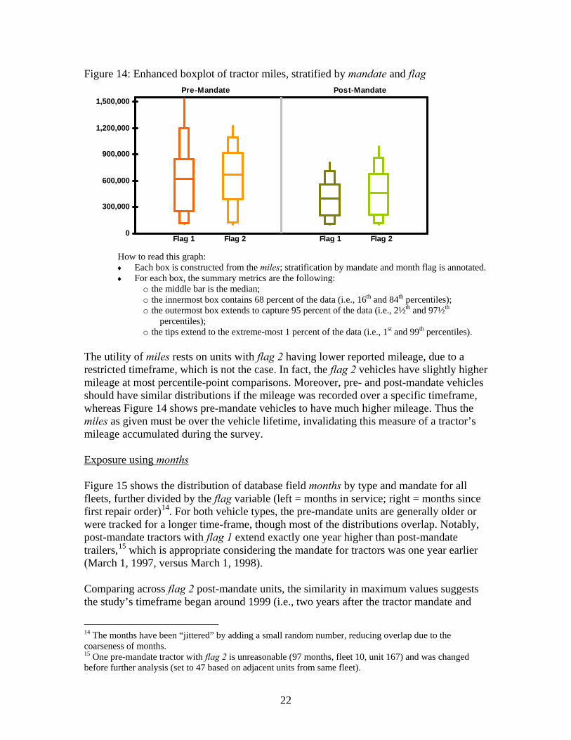
The validity of the given miles can be assessed relative to the month flag ie are miles recorded as total lifetime travel (flag 1) or since first repair order (flag 2) Figure 14 uses a form of boxplot to assess this question The vertical axis displays the miles as provided The left-hand pane contains pre-mandate units with post-mandate on the right Within each pane the left-hand box represents units with flag 1 with flag 2 to the right Each box has several demarcations to allow comparison across the distribution of miles the middle bar is the median the inner box contains 68 percent of the tractors the outer box contains 95 percent (cf normal distribution percentages) the extremities extend to include the upper and lower 1 percent
21
Figure 14 Enhanced boxplot of tractor miles stratified by mandate and flag Pre-Mandate Post-Mandate
0
300000
600000
900000
1200000
1500000
Flag 1 Flag 2 Flag 1 Flag 2
How to read this graph diams Each box is constructed from the miles stratification by mandate and month flag is annotated diams For each box the summary metrics are the following
o the middle bar is the median o the innermost box contains 68 percent of the data (ie 16th and 84th percentiles) o the outermost box extends to capture 95 percent of the data (ie 2frac12th and 97frac12th
percentiles) o the tips extend to the extreme-most 1 percent of the data (ie 1st and 99th percentiles)
The utility of miles rests on units with flag 2 having lower reported mileage due to a restricted timeframe which is not the case In fact the flag 2 vehicles have slightly higher mileage at most percentile-point comparisons Moreover pre- and post-mandate vehicles should have similar distributions if the mileage was recorded over a specific timeframe whereas Figure 14 shows pre-mandate vehicles to have much higher mileage Thus the miles as given must be over the vehicle lifetime invalidating this measure of a tractorrsquos mileage accumulated during the survey
Exposure using months
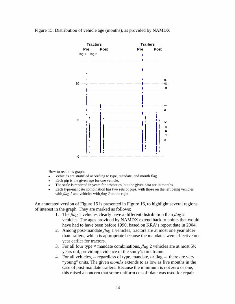
Figure 15 shows the distribution of database field months by type and mandate for all fleets further divided by the flag variable (left = months in service right = months since first repair order)14 For both vehicle types the pre-mandate units are generally older or were tracked for a longer time-frame though most of the distributions overlap Notably post-mandate tractors with flag 1 extend exactly one year higher than post-mandate trailers15 which is appropriate considering the mandate for tractors was one year earlier (March 1 1997 versus March 1 1998)
Comparing across flag 2 post-mandate units the similarity in maximum values suggests the studyrsquos timeframe began around 1999 (ie two years after the tractor mandate and
14 The months have been ldquojitteredrdquo by adding a small random number reducing overlap due to the coarseness of months 15 One pre-mandate tractor with flag 2 is unreasonable (97 months fleet 10 unit 167) and was changed before further analysis (set to 47 based on adjacent units from same fleet)
22
one year after the trailer mandate) The low-end (9 months) implies data collection ran up to around 2003 based on KRArsquos report date of February 19 2004 A reasonable guess at the studyrsquos time frame then is five-and-a-half years somewhere in the range March 1 1998 to December 31 200316 17 Among pre-mandate units those with flag 2 have an interesting ldquotricklerdquo pattern at the low end indicating that a few vehicles managed three years with no repairs or else joined the fleet at a later date as a used vehicle Pre-units with flag 1 curiously do not have this pattern but extend to minimum values at the same distribution as post-mandate and flag 2 units (these could be data-entry errors for example entry of years instead of months)
16 Envision a letter addressed to trucking fleets requesting maintenance receipts with a statement such as ldquoWe request that you provide records of repair expenses for all vehicles collected during the period March 1 1998 to February 28 2003rdquo 17 The youngest vehicles (5 months) would then have been purchased in late 2002 or early 2003 accruing some repair orders before the end of the survey A short amount of time should be factored in for KRA toperform the analysis as well
23
Figure 15 Distribution of vehicle age (months) as provided by NAMDX
Tractors Pre
Flag 1 Flag 2 Post
TrailPre
ers Post
10
5
A g e
i n y e
a r s
0
How to read this graph
diams Vehicles are stratified according to type mandate and month flag diams Each pip is the given age for one vehicle diams The scale is reported in years for aesthetics but the given data are in months diams Each type-mandate combination has two sets of pips with those on the left being vehicles
with flag 1 and vehicles with flag 2 on the right An annotated version of Figure 15 is presented in Figure 16 to highlight several regions of interest in the graph They are marked as follows
1 The flag 1 vehicles clearly have a different distribution than flag 2 vehicles The ages provided by NAMDX extend back to points that would have had to have been before 1990 based on KRArsquos report date in 2004
2 Among post-mandate flag 1 vehicles tractors are at most one year older than trailers which is appropriate because the mandates were effective one year earlier for tractors
3 For all four type times mandate combinations flag 2 vehicles are at most 5frac12 years old providing evidence of the studyrsquos timeframe
4 For all vehicles -- regardless of type mandate or flag -- there are very ldquoyoungrdquo units The given months extends to as low as five months in the case of post-mandate trailers Because the minimum is not zero or one this raised a concern that some uniform cut-off date was used for repair
24
Tractors Trailers Pre Post Pre Post
Flag 1 Flag 2
1 1
10
2
3 2 (flag 2)
5
4 (all)
0
V e h i c l e E
x p o s u r e (as given in years)Figure 16 Distribution of vehicle age (months) as provided by NAMDX annotated
Evidence that orders are time-sequential
receipts (eg June 31 2003) while the ages were back-calculated from some other date (eg December 31 2003) Inspection of the repair orders assuages this fear these ldquoyoungrdquo vehicles do have repairs later in sequence (based on the field orderid discussed more in following sections) although not at the extreme end and generally incurring multiple repair orders before the end of the survey
Further analysis is needed to determine if the months variable restricts the studyrsquos time-frame to approximately 1998 to 2003 as suggested by the dot plot above (Figure 15) If the earliest orders were performed on only pre-mandate vehicles this would indicate receipts were collected on some indeterminate time-frame perhaps beginning at some point before 1998 or possibly including a vehiclersquos entire in-service history An additional variable is used here the orderid which varies for each vehicle within the repair lines unlike months which has a single value for each vehicle As discussed in the section on adjustment procedures this orderid is presumably a grouping variable for repairs which were conducted at the same time though the precise definition of an ldquoorderrdquo might vary by fleet A crucial assumption is required the variable orderid is time-sequential within each fleet For example the order ldquo1000rdquo in Fleet 2 occurred
25
temporally before order ldquo2000rdquo although it can only be estimated how much earlier and nothing can be inferred regarding order ldquo2000rdquo for say Fleet 15
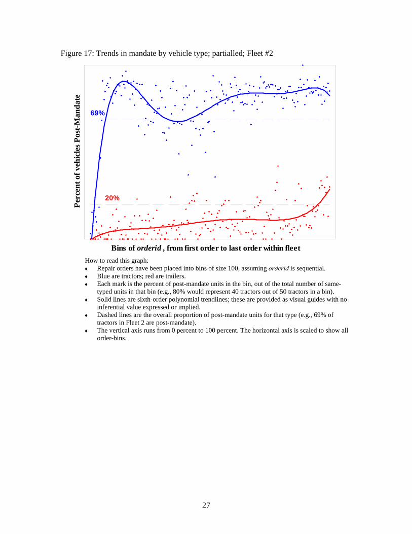
The graphics below (Figure 17 and Figure 18) shed light on the repair trends with respect to mandate Orders have been placed into class intervals of size 10018 assuming that orders are numbered sequentially within each fleet Blue dots are the percentage of tractor orders that are post-mandate (eg 40 of 50 tractor orders within the 100-block are post-mandate = 80) with red corresponding to trailers A high-order polynomial has been fit to each set to serve as a visual guide Overall fleet compositions are indicated by the dashed lines (ie within-fleet percentages from Table 1) In Fleet 2 for example post-mandate tractors experience more frequent repair orders than pre-mandate tractors relative to the overall fleet composition This is implied by the dashed line generally falling below the trendline and the bin data points the opposite is true for trailers
The samples below were selected because they are the two largest fleets Both fleets show an increasing presence of post-mandate tractors with respect to time Fleet 6rsquos trend is not monotone with respect to trailers while Fleet 2 shows a slower increase than in its tractors Grossly these trends hold across fleets post-mandate tractors become more prevalent with time while trailers are level or only slightly tilting towards newer units Most importantly the presence of post-mandate units at the earliest points indicates a closed interval for the survey rather than receipts representing a vehiclersquos full lifetime Further the survey began after the mandate took effect This has important implications for estimating vehicle exposure
The uneven distribution with time raises several additional points bull Repairs to post-mandate units may appear slightly more expensive on average due
to inflation bull Conversely pre-mandate units were older at the beginning of the study period
implying orders may have represented more substantial repairs bull Some combination of the following
o Pre-mandate units were retired during the period o Post-mandate units required little maintenance as brand-new vehicles but
required more repairs as they aged o New vehicles (post-mandate) entered the fleets
18 For example the first point summarizes orders 1 to 100 the second point summarizes orders 101 to 200 etc An alternate representation would be a moving average which would not change the nature of the analysis
26
Figure 17 Trends in mandate by vehicle type partialled Fleet 2
69
20
Perc
ent o
f veh
icle
s Pos
t-Man
date
Bins of orderid from first order to last order within fleet How to read this graph diams Repair orders have been placed into bins of size 100 assuming orderid is sequential diams Blue are tractors red are trailers diams Each mark is the percent of post-mandate units in the bin out of the total number of same-
typed units in that bin (eg 80 would represent 40 tractors out of 50 tractors in a bin) diams Solid lines are sixth-order polynomial trendlines these are provided as visual guides with no
inferential value expressed or implied diams Dashed lines are the overall proportion of post-mandate units for that type (eg 69 of
tractors in Fleet 2 are post-mandate) diams The vertical axis runs from 0 percent to 100 percent The horizontal axis is scaled to show all
order-bins
27
Figure 18 Trends in mandate by vehicle type partialled Fleet 6
37
4
Perc
ent o
f veh
icle
s Pos
t-Man
date
Bins of orderid from first order to last order within fleet
Adjustments to months
Table 2 shows the number of vehicles having the flag variable value of 1 and 2 for each fleet The high frequency of zero and other small values shows that the flag variable is dependent on the fleet A potential strategy for eliminating uncertainty about exposure would simply be to exclude the Flag 1 vehicles However as Table 2 shows exclusion of the Flag 1 vehicles would unduly weight the results towards those fleets which used Flag 2 If this were done Fleet 2 would dominate the analysis (eg 51 of pre-mandate trailers with Flag 2 are from Fleet 2) The retention of the Flag 1 vehicles will help this report maintain a more representative picture of maintenance expenditures for in-service vehicles in an uncontrolled setting
28
Table 2 Vehicle counts according to flag variable
Tractors Trailers Pre-Mandate Post-Mandate Pre-Mandate Post-Mandate
Fleet Flag 1 Flag 2 Flag 1 Flag 2 Flag 1 Flag 2 Flag 1 Flag 2 2 6 80 13 175 10 414 63 42 4 3 36 63 86 0 120 3 100 5 81 4 158 24 102 0 95 0 6 162 39 95 24 279 14 12 0 7 43 0 2 0 153 0 73 0 8 15 0 17 0 61 0 35 0 9 46 0 54 0 76 0 165 0
10 5 44 48 18 10 60 34 10 11 10 20 11 7 1 45 2 9 12 0 16 2 36 0 133 36 94 14 56 2 284 11 12 0 7 0 15 6 1 172 44 97 23 201 2
Total 433 242 919 425 801 809 725 257
Rather than ignoring a large number of vehicles potentially limiting generalizability and losing statistical power a system was devised to adjust the given months This analysis was conducted at the fleet level Examples are forthcoming The steps are as follows
0 Assume order IDs are sequential in time The field orderid is numeric
1 Calculate the relative position of each vehiclersquos first and last repair order within the fleet (0 to 1 scale)
2 Visually inspect months (as given) versus first repair order (lowest orderid) Look at overall patterns with an eye towards local linearity
3 When local linearity is violated adjust months for those vehicles that are out of line This means that ldquomostrdquo vehicles have acceptable months as given Generally when there are few vehicles to adjust or else the pattern has a
great deal of clustering vehicles are simply set to a certain value consistent with the pattern of that region
If linearity exists over a large area the adjustment is based on a linear interpolation (adjusted months are rounded to whole numbers for consistency)
4 Calculate a second value based on the difference between first and last order intended to approximate each vehiclersquos time in the survey
It is not clear if the provided months are from first to last repair order or from first repair order to the end of the survey19 The validity of this step is examined later
a) For example consider a vehicle with its first order at 010 and its last order at 090 (a difference of 080)
19 It could even be the case that the date-calculation reference date is different from the last date wherefrom receipts were collected
29
b) The value for months is 50 ndash this could be adjusted based on Step 3 above or could be the given value if it did not require adjustment
c) Months are truncated using the last orderrsquos relative position This is a quantitative approximate of the following verbal statement ldquoMost vehicles require regular maintenance If a vehicle did not incur any repair orders it was either not in the fleet or else was used so little that it did not require any Whatever the reason we should not lsquocreditrsquo these vehicles for time in service if they were not in userdquo For the hypothetical values in point (a) the following steps would be performed
i This vehicle was lsquoin the fleetrsquo for 80 percent of the total survey out of a maximum possible 90 percent based on the first order occurring at 010 and final order at 090
ii The age is scaled back by a factor of 8 to 9 89 times 50 = 444
iii One month is added to the adjustment (454) and rounded (45) serving two purposes
1 This prevents vehicles with a very small number of closely-spaced repair orders from having ldquozerordquo months
2 A vehicle is given a token amount of service-time after its final repair
iv If the ldquoadd onerdquo step makes this second adjustment higher than the first the value is lowered to the adjustment from the first step This can happen for vehicles with very late final repair
orders Rounding usually prevents this occurrence
The graphics below (Figure 19 ndash Figure 23) illustrate the adjustment process for Fleet 2 Figure 19 plots the given months against the first repair order
30
Figure 19 Given months versus first repair order (Fleet 2)
140
120
100
80
60
40
Mon
ths
(as
prov
ided
by
NAM
DX)
20
0 0 02 04 06 08 1
First order for each vehicle
Figure 20 contains the same data as Figure 19 with notation added to capture the trends in local linearity and highlight points which violate the trend Most points fall near the line segments Two groups are exceptions (1) vehicles with very early first repair orders and given months exceeding 50 up to 120 at the extreme (orange ellipses) and (2) a string of vehicles all given 36 37 or 38 months having first repair orders in the range 02 to 05 (green ellipse)
31
0
20
40
60
80
100
120
140
Mon
ths
(as
prov
ided
by
NAM
DX)
Figure 20 Given months versus first repair order (Fleet 2 highlighting trends and exceptions)
0 02 04 06 08 1First order for each vehicle
Figure 21 shows the results of adjusting those units noted in Figure 20 as being out of line with the fleetrsquos overall trend The vertical scale has been reduced to allow inspection of the linearity
32
0
5
10
15
20
25
30
35
40
45
50
Mon
ths
(adj
uste
d)
Figure 21 Adjusted months versus first repair order (Fleet 2 highlighting adjusted vehicles) (vertical scale reduced)
0 02 04 06 08 1
First order for each vehicle
Figure 22 (upper left) and Figure 23 (lower right) are zoomed-in versions of Figure 21 so that piecewise linearity can be further inspected Figure 22 shows that placing all high-valued points at 40 months fits well with the pattern in that region of the graph For practical purposes the alternative of interpolating on the range 45 to 35 would make little difference The adjusted vehicles with later first-repair orders (Figure 23) contribute to a trend that is as linear as one can reasonably expect Fourteen of the 19 vehicles in this region are post-mandate trailers with month flag 1 Speculatively these could have been purchased around the same time but incurred different usage patterns that caused some units to have much later first-repair orders (eg they were serviced by outside agents due to the types of routes undertaken or else were simply used little initially)
33
Figure 22 Adjusted months versus first repair order (Fleet 2 highlighting adjusted vehicles zooming in on upper left region)
000 002 004 006 008 010 012 014
First order for each vehicle
35
40
45
50
Mon
ths
(adj
uste
d)
34
Figure 23 Adjusted months versus first repair order (Fleet 2 highlighting adjusted vehicles zooming in on lower right region)
40
35
30
25
20 014 019 024 029 034 039 044 049 054
First order for each vehicle
Mon
ths
(adj
uste
d)
The next series of figures shows the adjustments for Fleet 5 While Fleet 2 required few adjustments (35 of 803 vehicles 4) Fleet 5 was more troublesome with 76 percent of vehicles (352 of 464) out of alignment Figure 24 shows the given months versus first repair order The problematic regions have been highlighted The upper portion is too high based on analysis of all fleets which suggests a survey timeframe of approximately five years (Figure 15) There is a lower cluster of vehicles with first repairs orders very close based on the order numbers but given ages varying over a wide range (14 to 43 months) An overall linearity is noted based on vehicles with early repair orders and months less than 60 along with a few having later repair orders and months around 40
35
Figure 24 Given months versus first repair order (Fleet 5 highlighting trends and exceptions)
0 02 04 06 08 1
First order for each vehicle
0
20
40
60
80
100
120
140
160
180
Mon
ths
(as
prov
ided
by
NAM
DX)
36
30
40
50
60
Mon
ths
(adj
uste
d)
Figure 25 Adjusted months versus First repair order (Fleet 5 highlighting adjusted vehicles) note reduction in scales for illustrative purposes
0 01 02 03 04 05 06
First order for each vehicle
Graphical analyses similar to those for Fleets 2 and 5 were conducted for all fleets Fleet 2 is typical of most fleets for the few vehicles requiring adjustment the steps are intuitively clear Fleets 5 and 15 have similarly troublesome patterns resulting in the most extreme uncertainty about how to perform the adjustments
The following list describes the adjustment procedure for two individual vehicles from Fleet 2 highlighted in Figure 26 The adjustment procedure includes establishing the time of the first and last repair order The actual exposure will be the difference between these two times
0 For fleet 2 there are 19536 orders 1 Relative order positions are calculated
a Unit ldquoTF433rdquo a pre-mandate tractor given 37 months with flag 2 frac34 First order at position 1882 AElig 1882 divide 19536 = 0096 frac34 Last order at position 10183 AElig 10183 divide 19536 = 0521
b Unit ldquo99793rdquo a post-mandate trailer given 39 months with flag 1 frac34 First order at position 10292 AElig 10292 divide 19536 = 0527 frac34 Last order at position 19255 AElig 19255divide 19536 = 0986
2 In Figure 26 the two sample vehicles are highlighted For ldquo99793rdquo the upper point (pink) is the given value and the lower value is the adjustment
37
0
20
40
60
80
100
120
140
TF433
99793
Mon
ths
(as
prov
ided
by
NAM
DX)
Figure 26 Adjustment procedure for two vehicles in Fleet 2
0 02 04 06 08 1 First order for each vehicle
a The given value for ldquoTF433rdquo falls within the overall pattern for the fleet thus it was not adjusted
b The given value for ldquo99793rdquo is higher than those with first repair orders around the same time thus it is lowered by a linear interpolation to 23 months (step 4)
3 Local linearity is evident in Figure 26 and was highlighted previously in Figure 20
4 The months are adjusted based on the first repair order For the two examples a Unit ldquoTF433rdquo does not require adjustment b Unit ldquo99793rdquo falls in the group with late first repair orders The months
were reduced according to the interpolation rounded to an estimate of 23 months
frac34 Linear interpolation according to point-slope form of a line y ndash y1 = m (x ndash x1) where y is the estimated months and x is the relative first order position20 AElig y = -325 (0527 ndash 014) + 36 = 234 AElig 23
5 The previous adjustment if any is further adjusted based on the final repair order (stage c on page 30) For the two examples
20 The slope is estimated from the points (014 36) and (054 23) with a corresponding slope of -13 divide 040 = -325 These points were selected from visual inspection rather than a regression analysis Either point placed back into the point-slope equation as (x1 y1) the first point was used in the calculation here
38
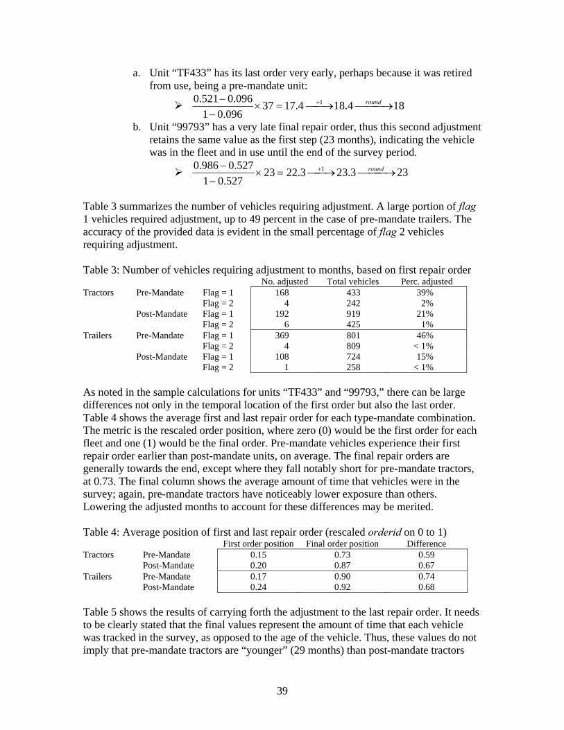
a Unit ldquoTF433rdquo has its last order very early perhaps because it was retired from use being a pre-mandate unit
0521minus 0096 +1 roundfrac34 times 37 = 174 ⎯⎯rarr184 ⎯ 18⎯⎯ rarr 1minus 0096
b Unit ldquo99793rdquo has a very late final repair order thus this second adjustment retains the same value as the first step (23 months) indicating the vehicle was in the fleet and in use until the end of the survey period
0986 minus 0527 +1 roundfrac34 times 23 = 223 ⎯⎯rarr 233 ⎯ 23⎯⎯ rarr 1minus 0527
Table 3 summarizes the number of vehicles requiring adjustment A large portion of flag 1 vehicles required adjustment up to 49 percent in the case of pre-mandate trailers The accuracy of the provided data is evident in the small percentage of flag 2 vehicles requiring adjustment
Table 3 Number of vehicles requiring adjustment to months based on first repair order No adjusted Total vehicles Perc adjusted
Tractors Pre-Mandate
Post-Mandate
Flag = 1 Flag = 2 Flag = 1 Flag = 2
Trailers Pre-Mandate
Post-Mandate
Flag = 1 Flag = 2 Flag = 1 Flag = 2
168 433 39 4 242 2
192 919 21 6 425 1
369 801 46 4 809 lt 1
108 724 15 1 258 lt 1
As noted in the sample calculations for units ldquoTF433rdquo and ldquo99793rdquo there can be large differences not only in the temporal location of the first order but also the last order Table 4 shows the average first and last repair order for each type-mandate combination The metric is the rescaled order position where zero (0) would be the first order for each fleet and one (1) would be the final order Pre-mandate vehicles experience their first repair order earlier than post-mandate units on average The final repair orders are generally towards the end except where they fall notably short for pre-mandate tractors at 073 The final column shows the average amount of time that vehicles were in the survey again pre-mandate tractors have noticeably lower exposure than others Lowering the adjusted months to account for these differences may be merited
Table 4 Average position of first and last repair order (rescaled orderid on 0 to 1)
Tractors Pre-Mandate 015 073 059 Post-Mandate 020 087 067 Trailers Pre-Mandate 017 090 074 Post-Mandate 024 092 068
First order position Final order position Difference
Table 5 shows the results of carrying forth the adjustment to the last repair order It needs to be clearly stated that the final values represent the amount of time that each vehicle was tracked in the survey as opposed to the age of the vehicle Thus these values do not imply that pre-mandate tractors are ldquoyoungerrdquo (29 months) than post-mandate tractors
39
(31 months) but rather that pre-mandate tractors were tracked in the survey for a shorter period of time on average (eg due to dis-use or scrappage)
Table 5 Averages for (1) given months (2) adjustment based on first repair order and (3) estimate of actual exposure based on first and last repair orders
Tractors Pre-Mandate 49 41 29 Post-Mandate 35 35 31 Trailers Pre-Mandate 48 40 36 Post-Mandate 36 36 33
Given (1) Adjustment (2) Actual Exposure (3)
(1) The values listed in the database from NAMDX ignoring the flag variable (2) The effect of linearizing the trend in months versus first repair order (3) Further adjustment of (2) to reflect the position of each vehiclersquos final repair order
The validity of the adjusted months is illustrated in Table 6 which is a portion of a correlation matrix relevant to this issue The given months first-order adjustment and actual exposure run across rows The columns show three measures of a vehiclersquos total repair exposure expense (total dollars across the survey) number of orders and number of repair lines First it is apparent that the given months do not correlate highly with the measures of repair orders for pre-mandate vehicles For the two stages of adjustment the adjustment based on both first and last repairs (ldquoActual Exposurerdquo in Table 5) has slightly higher correlations in all cases compared to the first-order adjustment Although most differences are slight this is a preponderance of evidence beyond chance (ie higher in 12 of 12 instances) While the given months are sufficient for post-mandate vehicles the second adjustment is used for all vehicles for the sake of consistency
Table 6 Correlations between various Months and measures of repairs Pre-Mandate Post-Mandate
Tractors (1) Given (2) Adjusted (3) Exposure
Trailers (1) Given (2) Adjusted (3) Exposure
Total $ No orders No lines Total $ No orders No lines (a) (b) (c) (a) (b) (c)
021 042 030 048 064 052 044 052 044 057 072 060 067 062 057 063 079 064 013 028 013 045 057 037 042 054 036 045 060 038 049 059 039 046 061 040
How to read this table diams This is a portion of a correlation matrix diams Columns are labeled as follows
(a) This is the total dollars in maintenance and repair expenses in the survey period (b) This is the number of repair orders that a vehicle required during the survey period (ie
the number of entries in the Orders table) (c) This is the total number of repair lines for each vehicle during the survey period (ie the
number of entries in the Repair Lines table) diams For example the correlation between the given months and the total repair expenses is 021
for pre-mandate tractors (upper left cell of table) diams Rows are labeled (1) (2) and (3) as in Table 5
40
Figure 27 Distribution of actual vehicle exposure adjusted based on first and last orders
Tractors Trailers Pre Post Pre Post
Flag 1 Flag 2
10
5
V e h I c l e E x p o s u r e (adjusted in years)
0
Cost inflation method
Figure 27 shows the distribution of actual vehicle exposure estimated based on both first and last repair orders The scale here is exaggerated to accentuate the difference to the ldquomonths in servicerdquo given in the database (Figure 15) namely the lack of pre-mandate units extending beyond 15 years If the Figure 15 values are used as the denominator (as they were in the unpublished 2004 report) the repair cost per month could be substantially underestimated especially for the pre-mandate vehicles The minimum values are also lower here because some vehicles had a small number of closely-spaced orders
Due to the length of the survey with some vehicles tracked for up to five years a method was devised to place the cost of each order in 2007 dollars It has been shown (eg Figure 17) that pre-mandate vehicles had more repair orders early in the timeframe and lower costs for these vehicles could reflect lower prices at the earlier times By placing all costs on a common baseline the comparisons become more comparable ndash oranges-toshyoranges as opposed to say oranges-to-grapefruits Each order was placed in its relative position on the 0 to 1 scale within fleet as described in the section on calculating actual exposure The maximum adjusted months was found
41
for each fleet ie the adjustment based on the first order but before calculating actual exposure based on both first and last order This maximum value for each fleet is assumed to represent the time from the beginning to the end of the survey period The maximum varies by fleet from 32 months (Fleet 9) to 65 months (Fleet 7) The survey timeframe is assumed to run until December 31 2003 for all fleets and the differences in age represent different starting points of data collection Taking the product of relative order position and maximum fleet age each order is placed into a year The costs for each order are adjusted using the Consumer Price Index21 with 2007 as the baseline22
Figure 28 shows the inflation calculation for two orders for the vehicle ldquoTF433rdquo from Fleet 2 (previously highlighted in Figure 26) The maximum months (not the exposure) for this fleet is 49 Counting backwards from December 31 2003 the year 2000 corresponds to orders in the range 002 to 027 and orders in the year 2001 fall in the range 027 to 051 The first sample order for this vehicle has a relative orderid of 0096 and is therefore placed in 2000 for the second sample the positions are 0458 and year 2001 Inflating to 2007 dollars the total cost of the first order increases by 20 percent to $168 from $140 The total cost of the second order increases by 17 percent to $230 from $197 These calculations are performed on all relative components as well eg brake costs are inflated at the order level from the approximated year of order to 2007
Figure 28 Inflation of two orders to 2007 dollars $197 x 117 = $230
2000 2001 2002 2003 2007
$140 x 120 = $168 (2000) (2007) inflate
21 Consumer Price Index httpwwwblsgovcpi calculations here are based on ldquoAll Itemsrdquo for ldquoAll Urban Consumersrdquo available at httpdatablsgovcgi-binsurveymostcu accessed January 16 2008 22 CPI data are provided with 1982-1984 as the baseline To set the baseline to 2007 the given value for 2007 (2073) is divided by the value for each year (eg 1799 in 2002) such that earlier years have values greater than one (eg 11523 for 2002) which represents the inflation (eg 1523 from 2002 to 2007)
42
To amortize expenses over a vehiclersquos lifetime the method found in the 1995 Economic Assessment of FMVSS Nos 105 and 12123 is adapted These calculations rely on two additional pieces of information (1) survival probability of heavy vehicles as a function of age and (2) vehicle miles traveled as a function of age These data are available from (1) RL Polk amp Corsquos vehicle registration counts (described in Appendix C) and (2) the Census Bureaursquos Vehicle Inventory and Use Survey (VIUS)24 These values should provide accurate estimates of lifetime expenses for tractors However there is no such data available for trailers and these same calculations are applied to both vehicle types The method is presented so that it could be applied in the existence of data specifically for trailers though at present the simplest solution is to apply the tractor data
Unfortunately there is no data on the extent that vehicle maintenance and repair expenses vary by age Though there are many scenarios two counteracting forces can be at work (a) vehicles incur more substantial repairs as parts age and (b) younger vehicles are given greater care in the form of preventive maintenance The extent to which these two factors neutralize each other can only be inferred by presenting several possibilities In reality the nature of vehicle maintenance is likely to vary by fleets for example due to the availability of capital to replace aging vehicles It is also unclear how maintenance expenses vary with age for specific vehicle systems which introduces further uncertainty in the reported values for the components of interest in this study
Table 7 shows the annual cash-flow discount factors for amortizing maintenance and repair expenses across a vehicle lifetime where the basis is $1 in year one These values apply across a population of all vehicles by incorporating survival probability The values should therefore be interpreted in terms of a large number of vehicles where some continue to accrue expenses over long time spans and others are decommissioned after several years
23 Final Rules FMVSS Nos 105 amp 121 Stability and Control During Braking Requirements and Reinstatement of Stopping Distance Requirements for Medium and Heavy Vehicles February 1995Accessible as FHWA-1997-2318-0022 24 Vehicle Inventory and Use Survey 2002 US Census Bureau Service Sector Statistics Divisionhttpwwwcensusgovsvsdwwwviusproductshtml
43
Table 7 Lifetime and Annual discount factors
Year VMT
(1)
Survival
(2)
Survival-Weighted
VMT (1 x 2)
Scenario X Per-mileage expenses constant Raw 3 7
Scenario Y Per-mileage expenses increase 10 annually Raw 3 7
1 100000 09995 99950 1 09848 09663 1 09848 09663 2 90000 09985 89865 1 08597 08119 110 09456 08931 3 81000 09953 80615 1 07487 06807 121 09060 08237 4 72900 09874 71979 1 06490 05680 133 08639 07560 5 65610 09747 63951 1 05599 04717 146 08197 06905 6 59049 09574 56531 1 04805 03897 161 07738 06275 7 53144 09354 49713 1 04102 03202 177 07268 05673 8 47830 09092 43488 1 03484 02618 195 06790 05102 9 43047 08790 37840 1 02943 02129 2 05887 04258
10 38742 08453 32747 1 02473 01722 2 04946 03444 11 34868 08083 28184 1 02066 01385 2 04133 02770 12 31381 07687 24124 1 01717 01108 2 03434 02216 13 28243 07270 20532 1 01419 00881 2 02838 01763 14 25419 06836 17377 1 01166 00697 2 02332 01394 15 22877 06392 14622 1 00953 00548 2 01905 01096 16 20589 05942 12233 1 00774 00429 2 01547 00857 17 18530 05491 10175 1 00625 00333 2 01250 00666 18 16677 05045 8414 1 00502 00257 2 01003 00515 19 15009 04608 6916 1 00400 00198 2 00801 00396 20 13509 04183 5651 1 00318 00151 2 00635 00302 21 12158 03774 4589 1 00250 00115 2 00501 00229 22 10942 03385 3704 1 00196 00086 2 00392 00173 23 9848 03017 2971 1 00153 00065 2 00306 00130 24 8863 02673 2369 1 00118 00048 2 00237 00097 25 7977 02353 1877 1 00091 00036 2 00182 00072 26 7179 02058 1478 1 00070 00026 2 00139 00053 27 6461 01789 1156 1 00053 00019 2 00106 00038 28 5815 01545 898 1 00040 00014 2 00080 00028 29 5233 01326 694 1 00030 00010 2 00060 00020 30 4710 01130 532 1 00022 00007 2 00045 00014 31 4239 00957 406 1 00016 00005 2 00033 00010 32 3815 00805 307 1 00012 00004 2 00024 00007 33 3434 00673 231 1 00009 00003 2 00018 00005 34 3090 00558 172 1 00006 00002 2 00013 00004 35 2781 00460 128 1 00005 00001 2 00009 00002 36 2503 00377 94 1 00003 00001 2 00007 00002
36+ 2253 00338 76 1 00003 00001 2 00005 00001
Sums 974968 796420 668 550 998 789
Several points of interpretation follow diams A lifetime of 36 years was selected in accordance with the 2006 reported on light
truck survival rates25 The1995 Economic Assessment used a lifetime of 25 years diams Column (1) is the vehicle miles traveled (VMT) estimated from the Census
Bureaursquos 2002 VIUS The magnitudes are not used explicitly in any calculations in part because the mileage in this study is not valid These values are used in
25 Vehicle Survivability and Travel Mileage Schedules S Lu September 2006 DOT HS 809 952
44
ratio form based on decreasing mileage of 10 percent per year Therefore the value of 100000 in year one is simply a baseline and could be listed as 10 or any other value26 Because of the way these mileage estimates are used a rigorous analysis was not conducted
diams Column (2) is the survival probability These estimates are based on tractor registrations from RL Polk amp Co The method is described in Appendix C These values should be more accurate than those in the 1995 Economic Assessment which were based on Polk data of light trucks rather than heavy trucks and values found in the Transportation Energy Data Book27 which were adopted from a method of the Federal Reserve and may therefore define survival in financial terms It is assumed that non-surviving vehicles accrue an average of one-half year of service during the year in which they are retired
diams The survival-weighted VMT (1 times 2) is the product of the two preceding columns It accounts for both the decreases in mileage and survival across the universe of heavy vehicles
diams Two scenarios for the trend in maintenance and repair expenses are presented o Scenario X assumes that the expenditure varies only in accordance with
the miles traveled the nature of repairs may change as vehicles age but mileage is the determinant of the expenses
o Scenario Y assumes that older vehicles require more costly maintenance and repairs as they age to the order of 10 percent more per mile driven per year up to the point where per-mile expenses are double that of a new vehicle Because this is on a mileage basis and multiplied by the survival probability the discount factors still decrease but do so less rapidly than in Scenario X In the Results section it is shown that pre-mandate (ie older)
vehicles have higher average monthly expenses It is not possible to fully justify the selection of 10 percent because there is no way to know how many miles the vehicles were driven during the survey period further complicated by knowing the true age of only flag 1 vehicles
A rough analysis was conducted only on the flag 1 vehicles by estimating the number of miles that would have been driven using the VIUS model of 10 percent decreases per year The results suggest that tractors have increasing per-mile maintenance expenses as they age (Scenario Y) but trailers are relatively flat with respect to age (Scenario X)
diams The column Raw shows the annual maintenance expenses per mile for those vehicles that survive
26 Flippancy should not be inferred from this statement 100000 miles in year one and 10 percent decreases thereafter produce a phenomenally strong fit for years 1 to 14 The empirical and modeled miles summed across these years differ by only 2 percent These estimates use the unweighted miles in VIUS which are not adjusted for partial-year operation of tractors Therefore the values reported here should more accurately represent the actual mileage driven as a function of age rather than a weighted value which treats all vehicles as if they were in operation for the full year 27 Transportation Energy Data Book Edition 26 2007 Oak Ridge National Laboratory httpctaornlgovdataindexshtml survival probability found in Table 3-10
45
diams Discount factors of 3 percent and 7 percent are reported as recommended by the Office of Management and Budget28
diams Discount factors represent the present value (PV) in 2007 where a new vehicle requires $1 of maintenance and repair expenses in year one
o The annual discount factors are calculated according to PV = FV (1 + i)-n
where FV is the future value of expenses i is the interest rate in decimal form eg 3 = 003 n is the mid-year time period eg year 2 is 15
o Future values (FV) account for the survival probability and decreasing mileage with age (Scenario X) with these decreases somewhat offset by assuming greater expenditures with vehicle age (Scenario Y)
o For example the column for 3 percent interest is constructed as follows In year 1 the present value is 1 times (1 + 003) -05 = 0985 In year 2 the expenses have decreased 10 percent due to lower
mileage making the present value 090 times (1 + 003) -15 = 0861 When survival begins to decrease ie after year 3 the present
values are also multiplied by the survival eg in year 10 the present value is 033949 times (1 + 003) -95 = 0256
When maintenance becomes more costly (Scenario Y) the values under Scenario X are increased by a compounded 10 percent eg in year 10 maintenance expenses have increased by 10 percent nine times (110 9 = 236) making the present value 0256 times 236 = 0604
diams The final row shows the sums across a 36-year lifetime o For example under Scenario X at 3 percent interest the value of 668
means that a fleet would expect an investment of $668 to account for the maintenance and repairs of 100 vehicles
28 Circular A-4 httpwwwwhitehousegovombcircularsa004a-4html
46
Initial observations and comments
bull ABS the average repair and maintenance costs specifically for ABS in post-mandate vehicles are $087 per month for tractors and $024 per month for trailers (inflated to 2007 economics) That is the principal finding of the analysis
o A small number of pre-mandate vehicles (40 of tractors 39 of trailers) had repairs to the ABS system and correct classification of these expenses was confirmed by inspecting the repair lines
o Comments from NHTSA engineers indicate that extremely few pre-mandate vehicles had ABS systems and these percentages should be smaller It could be that KRA mis-classified these vehicles but there is no evidence to support that claim
o Earlier NHTSA studies29 reported expenses of $125 per month for tractors7 and $211 per month for trailers8 when prices are inflated to 2007 dollars For tractors the result of the present study is 32 percent lower This could be due to differences in technology between in the approximately 10 years between surveys However the monthly expenses for trailers are substantially lower (88) nearly an order of magnitude It cannot be determined why the results are so discrepant between tractors and trailers
bull Brakes a key question is whether the presence of ABS has increased maintenance or repair to brake components beyond those that are specifically ABS-related The analysis shows that in fact overall brake repairs decreased from $3552 to $2678 per month in tractors and from $2193 to $1366 in trailers
o Based on these results the presence of ABS clearly did not increase maintenance or repair to brake components beyond those that are specifically ABS-related At the same time there is no basis for concluding that these observed decreases are due to ABS either It is
29 These comparisons refer to post-mandate vehicles because it is not accurate to compare the averages for the pre-mandate units in this study when very few vehicles had ABS systems
Results
Expenses per month of exposure
Table 8 shows the average monthly maintenance expenses per vehicle inflated to 2007 dollars
Table 8 Monthly Maintenance Expenses per vehicle expenses inflated to 2007 dollars at the order level (see also Figure 29 ndash Figure 33)
No of Vehicles Total Brakes ABS URG Tape
Tractors Pre-Mandate Post-Mandate
Trailers Pre-Mandate Post-Mandate
675 $525 $3552 $010 -- -- 1344 $499 $2678 $085 -- -- 1610 $151 $2193 $008 $017 $037 982 $143 $1366 $025 $014 $019
47
assumed that the addition of ABS to the overall brake system would not in itself lower maintenance and repair expenses That is the additional components would have their own direct expenses while potentially indirectly causing extra attention to be devoted to associated components Further because the ABS operation is not activated under normal braking conditions the presence of the ABS system should not alter the normal wear-and-tear patterns to the brake system as a whole which to a large extent contribute to the need for replacing and servicing brake parts Therefore the addition of ABS neither increased nor decreased maintenance or repair to brake components beyond those that are specifically ABS-related
bull Total repair and maintenance cost The total monthly expenditure for repairs to all vehicle subsystems decreased from $525 in tractors to $499 and from $151 to $143 in trailers
o These reductions (except within the brake systems) are unlikely to be related to ABS They presumably reflect that the post-mandate vehicles are newer on the average (in absolute age not necessarily exposure months during the survey) therefore in better condition and less in need of repair The newer vehicles would presumably accumulate greater mileage over a given time period (eg Table 7) making the differences even larger than what can be reported on a per-month basis
bull Brake repair as a proportion of total repair the proportion decreased from 68 percent ($3552 divide $525) in pre-mandate tractors to 54 percent in post-mandate It decreased from 145 percent to 96 percent in trailers This is further evidence that the addition of ABS did not result in an overall increase in brake repairs At the other end as with overall brake expenses it is not plausible that the addition of the ABS system would be the cause of lower brake expenses as a percentage of the total
o This result is checked against the parts expenses The proportion of brake parts expenses out of total parts expenses is 78 percent for pre-mandate tractors ($1845 divide $242) and 55 percent for post-mandate tractors ($1327 divide $233) For trailers the proportions are 189 percent ($1041 divide $5367) for pre-mandate units and 134 percent ($597 divide$3977) for post-mandate units These proportions are slightly higher than the proportions which included labor and service charges but the conclusions are not changed ndash pre-mandate vehicles devote a larger proportion of their total expenses to the brake system compared to post-mandate vehicles and trailers require relatively higher brake repair expenses compared to tractors
bull Underride guards ldquopre-mandaterdquo and ldquopost-mandaterdquo refer to the ABS mandate Because underride guards were required both before and after the ABS mandate repair costs are likely to be the same except to the extent that pre-mandate trailers are older
o Maintenance and repair costs are 16 cents per month in trailers combining ldquopre-mandaterdquo and ldquopost-mandaterdquo averages
o This item is not applicable to tractors as only the trailers are equipped with the guards
48
Figure 29 Monthly total expenses per vehicle by typemandate Monthly Total Cost per Vehicle (2007$)
$525 $499
$151 $143
Pre-Mandate Post-Mandate Tractors Trailers
bull Conspicuity tape here too ldquopre-mandaterdquo and ldquopost-mandaterdquo refer to the ABS mandate tape was required before and after Because tape runs the length of the trailer only a very small portion of the cost would be appropriate to allocate specifically to the URG
o In the older pre-mandate trailers cost for replacing worn-out tape averaged 37 cents per vehicle per month
o Cost in post-mandate trailers was smaller because few were old enough for the original tape to have worn out
o Tractors do not require sufficient lengths of tape to be applicable to this survey
49
Figure 30 Monthly brake expenses per vehicle by typemandate Monthly Brake Cost per Vehicle (2007$)
$3552
$2678
$2193
$1366
Pre-Mandate Post-Mandate Tractors Trailers
Figure 31 Monthly ABS expenses per vehicle by typemandate Monthly ABS Cost per Vehicle (2007$)
$085
$025 $010
$008
Pre-Mandate Post-Mandate Tractors Trailers
50
Figure 32 Monthly underride guard expenses per vehicle by typemandate Monthly Underride Cost per Vehicle (2007$)
$017
$014
Pre-Mandate Post-MandateTrailers
Figure 33 Monthly conspicuity tape expenses per vehicle by typemandate Monthly Tape Cost per Vehicle (2007$)
$019
$037
Pre-Mandate Post-MandateTrailers
Figure 34 shows the average brake expenses per vehicle as a percentage of the total maintenance expenses Although Figure 30 showed that both brake and total expenses are lower for post-mandate vehicles it could still be the case that the presence of the ABS system leads to increased brake expenses compared to the total expenses Here this is seen not to be the case where post-mandate units devote a lower percentage of their total expenses to brake repairs
51
Figure 34 Monthly brake expenses as a percentage of total monthly expenses by typemandate
Brake Expenses as a percent of Total Expenses
145
68
96
54
Pre-Mandate Post-MandateTractors Trailers
In reviewing the repair lines for orders with ABS charges it was noted which component required repairs Repair lines were classified as pertaining to the ECU wheel sensor or warning light Items classified as ldquoOthersrdquo are secondary components of the ABS system (eg valves and wires) or else were described too vaguely in the database to allow classification (eg ldquoCHECK ABSrdquo) A small number of orders listed repairs to two different components and these are counted in each column
Table 9 shows the number of orders per 100 vehicles on an absolute scale (ie not normalized on a monthly basis) for each of the ABS components Compared to trailers tractors required more frequent repairs to the wheel sensors and ECU Trailers more often required repairs of the warning light In sum the total number of items requiring repair is similar for tractors (210 per 100 vehicles) and trailers (193)
Table 9 Nature of ABS repairs (number of orders per 100 vehicles) Wheel Warning Sensor ECU Light Others Total
Tractors Pre-Mandate Post-Mandate
Trailers Pre-Mandate Post-Mandate
12 06 03 13 34 74 42 53 41 210 09 01 16 22 48 35 03 88 68 193
Lifetime expenses
Table 10 shows the estimated lifetime maintenance and repair expenses for the ABS system As described in the Methodology section (Table 7 page 44) there are two values used to discount the cash flow and two scenarios for the variation in maintenance expenses with age The discount rates of 3 percent and 7 percent were selected as recommended by the Office of Management and Budget28 The maintenance expenses
52
Table 11 Comparison of maintenance amp repair expenses to consumer cost for the ABS system (2007 dollars)
(A) (B) (A+B) (BdivideA) Consumer
Cost Maintenance
amp Repair Total
Tractor $639 $56 ndash 102 $695 ndash $741 9 ndash 16 Trailer $513 $16 ndash 30 $529 ndash $543 3 ndash 6 Connection $112 -- $112 --Total $1264 $82 ndash $132 $1346 ndash $1396 6 ndash 9
under Scenario X remain constant on a per-mile basis while under Scenario Y the per-mile expenses increase 10 percent per annum until they are double the initial costs The combination of Scenario Y with a 7 percent discount rate is the best single estimate30 but all values are displayed to provide a range
Table 10 Lifetime ABS maintenance amp repair net present value (2007 dollars) Discount Scenario X Scenario Y Rate
Tractors 3 $68 $102 7 $56 $81 Trailers 3 $20 $30
7 $16 $24
Table 11 combines the lifetime maintenance and repair expenses (column B) to the consumer costs (column A) cited in an earlier NHTSA report9 The ranges in column B represent the least-costly (Scenario X at 7) and most-costly (Scenario Y at 3) combination present in Table 10 All values are in 2007 dollars The final column (BdivideA) is the percentage that maintenance and repair add to the consumer cost The bottom row represents the purchase of a tractor and trailer in combination including the connection which was not analyzed in the current study
The most accurate lifetime maintenance and repair expenses for the underride guard are $18 based on all trailers combined ie there is no reason why classification as ldquopreshymandaterdquo or ldquopost-mandaterdquo in this study would make a difference in expenses This value could range from $14 to $20 for the different discount rates and scenarios as presented for the ABS system The lifetime expenses for conspicuity are estimated as $35 ranging from $24 to $44 This is based on the pre-mandate trailers because the post-mandate trailers would be unlikely to have accumulated a great deal of wear and tear in (at most) six years of use The consumer costs have not been evaluated by NHTSA
30 Pre-mandate vehicles in this study had higher average monthly costs and were likely driven fewer miles during the timeframe as suggested by VIUS The 7 percent interest rate represents the average pre-tax return on investment in the private sector and is used as the standard value in most financial analyses See for example sect7d of the FHWArsquos Procedural Guidelines for Highway Feasibility Studies httpwwwfhwadotgovhep10corborfeastudyhtml
53
Fleet differences
From the outset it was acknowledged that fleets vary in vehicle-type composition31 and potentially in vehicle use and maintenance policies In this section the validity of the results with respect to type and mandate is assessed to ensure that results are consistent within each fleet Figure 35 portrays the average monthly total maintenance per vehicle Each family of bubbles is one fleet with pre-mandate units to the left and tractors to the top as are most charts throughout the report Three fleet characteristics are depicted according to KRArsquos classification scope vocation and size (the latter represented by the font size of the fleetid label) The lower right family represents the average across all fleets and the ldquo$250rdquo bubble is included for size reference
31 Refer to Table 1 on page 9
54
Figure 35 Monthly total expenses per vehicle by typemandate classified by Fleet according to vocation scope and size
2 5
6
9
1112
10 14 15
4
7
8
$250
All Fleets
Truckload LTL Specialized Dedicated
West
East
Continental
Trans-Continental
How to read this figure diams The summary statistic is the mean monthly maintenance cost per vehicle
o The area of each bubble is proportional to the cost diams Each fleet is represented by a set of four bubbles
o The lower pair are trailers the upper pair are tractors o The left-side pair are pre-mandate the right-side pair are post-mandate
diams The mean across ldquoAll Fleetsrdquo is included at the bottom right o The bubble ldquo$250rdquo provides scale
diams Fleet numbers are listed above or below each fleet diams Three fleet characteristics are depicted as defined by NAMDX
o Scope is the vertical classification (West etc) o Vocation is the horizontal classification (truckload etc) o Size is represented by the font size of the fleet number (small medium large)
Figure 35 simply illustrates that differences exist between fleets Without knowledge of the operating conditions and maintenance procedures for these twelve fleets it is not possible to form conclusions about the reasons for this variability The small number of fleets is insufficient to draw conclusions with respect to scope vocation and size For example Fleet 7 is the only eastcoast and the only less-than-load fleet and it is one of only two small fleets (along with Fleet 8) Inferences drawn in regards to these classifications would be unable to unravel whether differences between Fleet 7 and others are due to scope vocation size or simply idiosyncrasies in that fleetrsquos maintenance policies
55
The differences in fleet composition could give rise to Simpsonrsquos Paradox32 This occurs when the directionality of overall means differs from the directionality of individual group means For example a basketball coach wants to know which of two players is a more accurate shooter The number of shots converted and attempted are shown in Table 12 for two games Player B made a higher percentage of his shots in each game while Player A made a higher percentage overall Each player also made 40 percent more of his shots in Game 2 compared to Game 1 The grouping variable ldquoGamerdquo invokes differing weights (ie the number of shots taken) in computation of the total average
Table 12 Illustration of Simpsons Paradox Game 1 Game 2
Player A 5 of 10 (50)
18 of 20 (90)
Player B 12 of 20 (60)
10 of 10 (100)
Total 23 of 30 (77) 22 of 30 (73)
The intent here is not to determine where Player A or Player B is a better shooter Such a decision could rest on other factors such as the quality of teams played in Game 1 and Game 2 Context and subject matter knowledge are crucial The example merely illustrates the arithmetical possibility of Simpsonrsquos Paradox
For the present analysis differences in fleet means (Figure 35) and type times mandate composition (Table 1) could give rise to Simpsonrsquos Paradox Table 13 shows how this might occur simplified to the case of one vehicle type for two fleets The data are average monthly total maintenance expenses Each fleet has a higher average for post-mandate vehicles while the overall average is higher for pre-mandate vehicles The disparate conclusions arise from differences in number of vehicles
Table 13 Hypothetical case of Simpsons Paradox Fleet A Fleet B Total
Pre-Mandate $400 (400)
$200 (100)
$360 (500)
Post-Mandate $500 (100)
$300 (400)
$340 (500)
For the real data the combined data across fleets (Table 8 and Figure 29) showed that pre-mandate vehicles had higher total monthly costs than post-mandate vehicles and that tractors had higher costs than trailers From lowest to highest the data were ranked (1) post-mandate trailers (2) pre-mandate trailers (3) post-mandate tractors and (4) pre-mandate trailers It is important that this pattern hold across fleets illustrated in Figure 36 There are four sets of blocks each containing the within-fleet rank of average by type times mandate Each set contains 12 digits corresponding to the 12 fleets Critically the rank-orders within fleet show few exceptions to the overall pattern Ideally each block would have the same digit occurring throughout (eg all 4 in the upper left for preshy
32 httpenwikipediaorgwikiSimpsons_paradox
56
mandate tractors) The differences are fortunately minimal implying that the grouping variable ldquoFleetrdquo does not give rise to Simpsonrsquos Paradox
Figure 36 Rank orders of total expenses per month by fleet (4 = highest)
44 4 4
4 4 4 4
4 4 4 4
3 3 3 3
3 3 3 3
3
3 33
22 2 2
2 22 2
2
2 2 2
1 1 11
11 1 1
1 1 1 1
Pre-Mandate Tractors Post-Mandate Tractors
Pre-Mandate Trailers Post-Mandate Trailers
The fleet rank orders for brake expenses per month (Figure 37) and brake expenses as a percentage of total expenses (Figure 38) are not as consistent as those for total expenses per month This is in part due to the fact that post-mandate tractors had only slightly higher monthly brake expenses than pre-mandate trailers (Figure 30) though this comparison is not one of particular interest
57
Figure 37 Rank orders of brake expenses per month by fleet (4= highest)
44 4 4
4 4 4 4
4 4
4
4
3 3
3
3
3 3
3
3
3
3
33
22
2
2
2
2 2
2
22
2
2
1 1 1 1
1
1
1 1
1
1
11
Pre-Mandate Tractors Post-Mandate Tractors
Pre-Mandate Trailers Post-Mandate Trailers
58
Figure 38 Rank orders of brake expenses as a percentage of total expenses by fleet (4= highest)
4 4 4 4
4 4 4 4
4 4 44
3
3
3 3
3
3 3 3
3 3
3 3
2
2
2 2
2
22 2
2 2
22
1 1 1 1
11 1 1
1 11 1
Pre-Mandate Tractors Post-Mandate Tractors
Pre-Mandate Trailers Post-Mandate Trailers
The patterns in the above figures can be tested statistically using the exact binomial test33 For each vehicle type a tally is made of the number of fleets where the post-mandate costs are lower than the pre-mandate costs The tallies are compared to an expectation of 50 percent (6 out of 12) equivalent to flipping a fair coin The p-value is a quantitative assessment of the strength of the evidence against the 50 percent assumption A result of 10 out of 12 is significantly different from 50 percent at the generally accepted level of α lt 005 while 9 out of 12 can be considered marginally significant at α lt 010
Table 14 shows the results of the exact binomial test based on the rank-order of expenses within each fleet Four of the six metrics indicate lower expenses for post-mandate vehicles at a statistically significant level of α lt 005 while the other two metrics are marginally significant at α lt 010 Taking the ldquototal per monthrdquo for tractors as an example the results are interpreted as follows ndash the post-mandate vehicles had lower expenses than the pre-mandate vehicles in 10 of the 12 fleets and this occurrence is
33 A binomial calculator can be found at httpwwwstattamuedu~westappletsbinomialdemohtml
59
unlikely compared to an assumption that expenses should be equal for pre-mandate and post-mandate tractors
Table 14 Summary of fleet rank-order statistical tests (based on 12 total fleets) Post-Mandate Metric Lower Binomial Test p
Tractors
Trailers
Total per month Brake per month
Brake as of Total
10 10 9
0019300193 0 0730
Total per month Brake per month Brake as of Total
9 10 11
00730 0 0193 0 0032
Inferential analysis of cost differences
This section describes an inferential analysis of the total cost per month brake cost per month and brake cost as a percent of total cost The intent is to demonstrate whether the differences between pre-mandate and post-mandate vehicles are statistically significant
Because the costs are positively-skewed standard statistical methods based on parametric assumptions may be invalid Figure 39 shows a histogram of the monthly total cost per vehicle The distributions for brake costs per month and brake cost as a percentage of total cost have distributions of the same general shape
60
Figure 39 Histogram of monthly total cost per vehicle Number of Vehicles
770741
513
375
308
219 204 167 176 171
149 159 136
101 96 76 63 50 53
38 14
$0 $50
$100
$150
$200
$250
$300
$350
$400
$450
$500
$550
$600
$650
$700
$750
$800
$850
Over $9
00$1000 $9
50
$100
0$1
000
$105
0
$110
0
How to read this graph diams Monthly total cost per vehicle is counted in bins of $50 eg the 2nd bar represents $50 to
$100 diams The number atop each bar is the frequency of vehicles in that bin diams Bins extend consecutively up to $1000 per vehicle diams The rightmost bar represents vehicles with costs above $1000 The extra spacing is stylistic
and does not imply empty bins
A non-parametric procedure was developed to mitigate violations of distributional assumptions The ability to control for fleet differences is desirable as well (Figure 35) The procedure is as follows
1 All vehicles are ranked according to total cost per month In the rare event of ties the mean rank is used (eg a tie at positions 500 and 501 would assign 5005 to each vehicle)
2 On the ranked data ANOVA is conducted The model includes type mandate the type-mandate interaction and fleetid In SAS proc glm is used
3 The least-squared means (lsmean) are requested for type times mandate controlling for fleetid This essentially gives a ldquomean of the meansrdquo based on fleet averages for each type times mandate rather than the grand means
61
4 The lsmean for each type-mandate combination is back-mapped to the unshyranked total costs For example an lsmean of 1000 would be mapped to the vehicle with the 1000th highest total cost ignoring type and mandate
Table 15 and Table 16 summarize the overall model effects for total and brake costs Other sub-costs are not presented because the excess of zeroes make the data too skewed
Table 15 Model results for total Cost per month Source F (df1 df2) p Fleet 109 (11 4595) lt 00001 Type 2943 (1 4595) lt 00001 Mandate 112 (1 4595) lt 00001 Type times Mandate 37 (1 4595) 0055
Table 16 Model results for brake Cost per month Source F (df1 df2) p Fleet 107 (11 4595) lt 00001 Type 393 (1 4595) lt 00001 Mandate 355 (1 4595) lt 00001 Type times Mandate 40 (1 4595) lt 00001
Table 17 Model results for brake Cost as a percentage of total Cost Source F (df1 df2) p Fleet 51 (11 4595) lt 00001 Type 86 (1 4595) lt 00001 Mandate 238 (1 4595) lt 00001 Type times Mandate 49 (1 4595) lt 00001
All effects are highly significant with p lt 00001 for all cases except the interaction on total Cost (p = 00019) Because the type times Mandate interactions are significant cell means (adjusted for fleet) are compared There are six possible comparisons based on four combinations of vehicle and mandate Therefore use of the standard α = 005 for comparisons will inflate the overall error rate Only four comparisons are of interests out of the possible six because there is no need to compare across type and mandate (eg do not compare pre-tractors to post-trailers) The formula below is used to calculate an appropriate alpha level The solution is 00127
1 ndash (1 ndash α) 4 = 005
Figure 40 and Figure 41 summarize the findings of this analysis for total and brake costs The ranking procedure reduces the scale more akin to an analysis on medians rather than means The patterns for both total and brake costs are similar to those for raw averages (cf Figure 29 and Figure 30) with the differences slightly more pronounced here All differences of interest are statistically significant (p lt 00127) represented by dashed lines rather than solid lines to signify statistical inequality
62
Figure 40 Fleet-adjusted non-parametric monthly total cost per vehicle (2007$) Monthly Total Cost per Vehicle
(Non-Parametric Fleet-Adjusted 2007$)
$452
$370
$133 $95
Pre-Mandate Post-Mandate Tractors Trailers
Figure 41 Fleet-adjusted non-parametric monthly brake cost per vehicle (2007$) Monthly Brake Cost per Vehicle
(Non-Parametric Fleet-Adjusted 2007$)
$588
$1647 $1592
$2432
Pre-Mandate Post-Mandate Tractors Trailers
How to read this graph diams Analysis is performed on the ranked data as described on page 61 diams Reported values are the fleet-adjusted least-squared means from proc glm in SASdiams Comparisons of interest are connected by dashed lines representing significant differences diams Comparisons are not made across the type-mandate combinations (ie do not compare pre-
tractors to post-trailers and vice versa) diams The ranking procedure reduces the magnitudes compared to the means
The analysis conducted on brake costs as a percentage of total cost (Figure 42) leads conclusions in the same manner as analysis of costs per month Again post-mandate vehicles have lower values The difference here as in Figure 34 is that trailers require a
63
Figure 42 Fleet-adjusted non-parametric brake cost as a percentage of total cost Brake Cost as a percentage of Total Cost per Vehicle
(Non-Parametric Fleet-Adjusted)
99
62 51
47
Pre-Mandate Post-Mandate Tractors Trailers
higher percent of their maintenance and repair expenses for brakes because the total expenses for trailers is so much lower than for tractors
64
Appendix A VRMS codes
A1 Vehicle systems
First section of codes often given in 2-digit format (eg 001 is the same as 01) from httpwwwtruckrealmcomvmrshtm
Cab Climate Control Instrumentation and Aerodynamic Devices 001 Air Conditioning Heating and Ventilating System002 Cab and Sheet Metal003 Instruments Gauges (All) and Meters004 Aerodynamic Devices
Chassis 011 Axles FrontmdashNon-Driven012 Axles RearmdashNon-Driven 013 Brakes014 Frame 015 Steering 016 Suspension017 Tires 018 Wheels Rim Hubs and Bearings019 Automatic Chassis Lubricator
Drivetrain 021 Axle DrivenmdashFront Steering 022 Axle DrivenmdashRear 023 Clutch 024 Drive Shaft(s) 025 Power Take Off 026 TransmissionmdashMain Manual027 TransmissionmdashMain Automatic 028 TransmissionmdashAuxiliary and Transfer Case 029 Auxiliary Section (TransmissionmdashMain Manual)
Electrical 031 Charging System032 Cranking System033 Ignition System034 Lighting System
Engines Code System041 Air Intake System042 Cooling System043 Exhaust System044 Fuel System045 Power Plant046 Electric Propulsion System047 Filter Kits (Multi-Piece)
65
Accessories 051 General Accessories (for power units trailers etc) 052 Electrical Accessories (for power units trailers etc) 053 Expendable Items (for power units trailers etc) 054 Horns and Mounting and Reverse Signal Alarms055 Cargo Handling Restraints and Lift Systems (for power units trailers etc) 056 Power Take Off 057 Spare Wheel Mounting 058 Winch (for power units trailers etc) 059 Vehicle Coupling
Special Applications 061 Terminal Equipment Systems and Accessories 065 Hydraulic Systems
Bodies and Vessels071 Body (except bulk carrier body) 072 Rear Wall and Door 073 Tank Vessel inner shell074 Tank Vessel outer jacket075 Manholes076 Rings and Bolsters 077 Trailer Frame and Support078 Trim and Miscellaneous Hardware 079 Safety Devices
Heating and Refrigeration081 Heating Unit (for power units trailers etc) 082 Refrigeration Mechanical (for power units trailers etc) 083 Refrigeration Nitrogen (for power units trailers etc) 084 Refrigeration Holdover Plate (for power units trailers etc)
Bulk Product Transfer Systems 091 Blowers Conveyors and Vibrators (for power units trailers etc) 092 Compressor Bulk Product Systems (for power units trailers etc) 094 Engine Auxiliary (for power units trailers etc) 095 Manifold (for power units trailers etc) 096 Power Shaft (for power units trailers etc) 097 Pump (for power units trailers etc) 098 Valves and Controls (for power units trailers etc) 099 Safety Devices Instruments and Gauges (for power units trailers etc)
A2 Brake Components
Second section of code for 013 Brakes (most common description occurrences in repair-line file)
13-001 FRONT BRAKES amp DRUMS 13-002 REAR BRAKES amp DRUMS 13-003 PARKING BRAKES 13-004 BRAKE CHAMBER 13-005 ltuncertaingt (13-005-001 is BEARING all others low frequency) 13-006 MASTER CYLINDER
66
13-007 BRAKE LINES amp FITTINGS - HYDRAULIC amp AIR 13-008 (infrequent subcodes indicate valves or hoses) 13-009 AIR COMPRESSOR 13-010 SEAL-GLAD HAND 13-011 ltABS-related see belowgt 13-012 BRAKE KIT (several variants)
A3 ABS assemblies
Third section of code for 013-011 ABS subsystem (items BOLD are those most common)
13-011-001 BRAKE ROTOR 13-011-002 ABS SENSOR 13-011-003 BRACKET ndash SENSOR 13-011-004 CABLE 13-011-007 SWITCHES 13-011-009 CLIP - ABS SENSOR 13-011-066 RELAY - ELECTRICAL ANTILOCK 13-011-067 SENSOR LOCK 13-011-068 ABS RELAY VALVE 13-011-069 CONTROLLER - ELECTRONIC ANTILOCK 13-011-070 CABLE ndash ABS 13-011-071 ABS MOD VALVE and VALVE ECU ABS 13-011-072 VALVE 13-011-073 SENSOR - ABS 13-011-076 ELEC CONTROL UNIT (or similar) 13-011-077 TRACTION CONTROL VALVE 13-011-078 SWITCHES (shortened) 13-011-079 ABS LIGHT 13-011-080 CONNECTOR - ELECTRICAL SPEED SENSOR 13-011-096 HARNESS-MODULATOR VALVE 13-011-107 RELAY VALVE or DASH VALVE 13-011-108 RELAY VALVE
67
Appendix B Probability of Survival
Two sources for vehicle survival were uncovered (1) the 1995 Economic Assessment23
used values derived from RL Polk amp Co data but these were based on light trucks and (2) the Transportation Energy Data Book27 based its data on a method derived from the Federal Reserve for determining scrappage rates which might be based on financial calculations rather than the actual number of vehicles in service
A method was devised to determine a more accurate survival timeline for the vehicles in this study Data from Polk were used here except that they were specifically filtered to include only tractors Polk reports the number of registered vehicles by make model and model year among other variables The annual survey is a snapshot on July 1 of the respective year Due to timing of model-year production and sales of vehicles there is lag in vehicles entering the registration database For example the survey year 2005 contains counts of model years up to 2006 However the counts for 2005 and 2006 are not usable because of time involved in the production-sale-registration process The most recent model year therefore with valid counts from the 2005 survey would be 2004 The survey year 2005 thus becomes the baseline (age 0) for model year 2004 vehicles (114501 in number) The 2006 survey then gives the number of 2004 model year vehicles surviving to year 1 (110486) The year-to-year ratio is the survival estimate to year 1 (110486 divide 114501 = 0965)
Survival probabilities are calculated on a moving basis That is each annual rate is determined eg years 1-to-2 years 2-to-3 3-to-4 etc These are conditional probabilities ie the probability of surviving to year N +1 given that the vehicle was present in year N
The Polk survey years from 1997 to 2006 were used (there may have been a change in methodology from earlier years because 1996 counts appear too high in some instances) Each annual survival rate thus has nine values For example survival from year 1-to-2 can be calculated using model years 2003 (ratio of 2006 to 2005 survey counts) down to 1995 (ratio of 1998 to 1997 counts) The nine values are averaged and become the estimate of the survival probability from year N to N + 1
Model year counts are available back to 1975 This gives a maximum vehicle age of 30 years using the ratio of 1975 model year counts from the 2006 survey to that of the 2005 survey However the advanced ages have fewer estimates to use in the average In the case of 30 years there is only this one estimate For age 29 there are two estimates etc For all ages below 23 nine values are used in the average Calculating survival probability up to year 25 is reasonable though further extensions are purely model-based (discussion forthcoming)
To determine the probability of a vehicle surviving through year X the individual year-to-year probabilities are multiplied up to and including year X For example the probability of a tractor surviving through year 10 is the product of survival from year 0shy
68
to-1 1-to-2 hellip 9-to-10 This method is compatible with that used in epidemiology for construction of a life table34 for example as the CDC reports for the human life expectancy35 such as in Table 18 The outcome of the present analysis is to produce this same type of table for tractors
Table 18 Life Table for humans reproduced from CDC data
Total Personshy
Probability Number years number of person-
of dying Number dying lived years Expectation surviving
between to between between lived above of life ages x to ages x to ages x to
x+1 age x x+1 x+1 age x at age x Age q(x) l(x) d(x) L(x) T(x) e(x)0-1 0006865 100000 687 99394 7743016 774
1-2 0000469 99313 47 99290 7643622 770
2-3 0000337 99267 33 99250 7544332 760
3-4 0000254 99233 25 99221 7445082 750
4-5 0000194 99208 19 99199 7345861 740
5-6 0000177 99189 18 99180 7246663 731
6-7 0000160 99171 16 99163 7147482 721
7-8 0000147 99156 15 99148 7048319 711
8-9 0000132 99141 13 99134 6949171 701
9-10 0000117 99128 12 99122 6850036 691
10-11 0000109 99116 11 99111 6750914 681
11-12 0000118 99105 12 99100 6651803 671
12-13 0000157 99094 16 99086 6552704 661
13-14 0000233 99078 23 99067 6453618 651
14-15 0000339 99055 34 99038 6354551 642
15-16 0000460 99022 46 98999 6255513 632
16-17 0000577 98976 57 98947 6156514 622
17-18 0000684 98919 68 98885 6057566 612
hellip 94-95 0192080 10519 2021 9509 38901 37
95-96 0207636 8499 1765 7616 29392 35
96-97 0224075 6734 1509 5980 21776 32
97-98 0241387 5225 1261 4594 15796 30
98-99 0259552 3964 1029 3449 11202 28
99-100 0278539 2935 818 2526 7752 26
100+ 100000 2118 2118 5226 5226 25
The columns are defined and calculated as follows diams x is the beginning Age eg x = 0 on the first row
34 httpenwikipediaorgwikiLife_table 35 The direct link to the 2003 Life Table is httpwwwcdcgovnchsdatanvsrnvsr54nvsr54_14pdf The linking page at httpwwwcdcgovnchsfastatsdeathshtm is a better resource for readers seeking newer information
69
diams q(x) is the probability of dying (failing to survive) This is empirical All other columns are calculated from this value
diams l(x) is the number surviving to age x with a baseline of 100000 newborns o l(x) = (1minus q(x minus1))times l(x minus1)
diams d(x) is the number dying in the year beginning xo d (x) = q(x)l(x)
diams L(x) is the number of person-years lived (or tractor-years in service) by individuals alive at the beginning of age x It is assumed that deaths during age x occur on-average at the middle of year (except at age 0 where more deaths occur very close to the beginning ie neonatal)
1o L(x) = l(x) minus d (x)
2 diams T(x) is the number of years lived including and beyond age x eg T(10) is the
number of cumulative person-years lived from years 10 to infinity infin
o T (x) = sumL(a) a=x
diams e(x) is the life-expectancy for an individual alive at year x eg e(10) is the expected number of years of life remaining for a 10 year-old individual (681)
o e(x) = T (x) divide l(x)
The survival probability to the end of year x can be taken as the ratio of the number surviving l(x) to the baseline population of 100000 It can be calculated by multiplying the individual-year survival rates as follows
xminus1
S(x) =prod(1minus q(a)) a=0
Table 19 applies these methods to the Polk data for tractors When this same method is applied to data for passenger cars the survival probabilities are within one percent of those reported in the 2006 report up to year 11 Such strong agreement suggests the method applied in this report is valid
70
Table 19 Life Table for tractors unadjusted Total
Probability Number Tractors-years number of of
retirement Number retired in service tractors-years Expectation between surviving to between between in service above of life ages x to
x+1 age x ages x to x+1 ages x to x+1 age x at age x Age q(x) l(x) d(x) L(x) T(x) e(x)
0-1 0031446 100000 3145 98428 1755719 176
1-2 0024134 96855 2338 95687 1657291 171
2-3 0001563 94518 148 94444 1561605 165
3-4 0002227 94370 210 94265 1467161 155
4-5 0012030 94160 1133 93594 1372896 146
5-6 0023950 93027 2228 91913 1279302 138
6-7 0029246 90799 2656 89471 1187389 131
7-8 0035618 88144 3139 86574 1097918 125
8-9 0036581 85004 3110 83449 1011344 119
9-10 0040060 81895 3281 80254 927894 113
10-11 0045155 78614 3550 76839 847640 108
11-12 0047910 75064 3596 73266 770801 103
12-13 0056960 71468 4071 69432 697535 98
13-14 0068821 67397 4638 65078 628102 93
14-15 0068906 62759 4324 60596 563024 90
15-16 0073576 58434 4299 56285 502428 86
16-17 0077821 54135 4213 52028 446143 82
17-18 0081691 49922 4078 47883 394115 79
18-19 0084807 45844 3888 43900 346232 76
19-20 0099516 41956 4175 39868 302332 72
20-21 0085609 37781 3234 36163 262464 69
21-22 0104579 34546 3613 32740 226300 66
22-23 0114099 30933 3529 29169 193560 63
23-24 0127171 27404 3485 25661 164392 60
24+ 1000000 23919 23919 138730 138730 58
An interesting phenomenon is what might be described as ldquoinfant mortalityrdquo of tractors ndash the probability of removal from the registration rolls is high initially and reaches a minimum after year three then increases (nearly) monotonically throughout the lifetime Taking these values literally would imply the analog of ldquochildhood diseasesrdquo which might be catastrophic mechanical failures during the first three years resulting from poor manufacture Considering that passenger cars do not exhibit this curiosity25 a more likely scenario is that variability in registration policies and procedures causes some vehicles to move in-and-out of registered status during the first few years The cause of this phenomenon is beyond the scope of the present report
Because the probabilities are multiplicative application of the higher retirement rates during the first three years would (slightly) lower survival for all ages These values have been fixed as 0999 which would mean that only 1 in 1000 vehicles are retired in each of the first two years This would generally represent vehicles involved in totality accidents It also occurs occasionally that the number registered vehicles increases from one survey
71
year to the next leading to a survival probability of greater than one This is sufficiently rare that the average survival rates in Table 19 are all less than one When survival probabilities are greater than one they are reset to exactly one before being averaged with other values for that age
Table 20 shows the life table for tractors which was used in calculations of the lifetime discount factors in Table 7 To eliminate noise in the data the year-to-year retirement rate from year three onwards was modeled by a function of the form p(t) = A ebt + c The constant c was assumed to be 0001 representing a constant rate for the probability of involvement in totality accidents The constants A and b in the time-varying term were found using Solver in Microsoft Excel A sum-of-squares discrepancy function served as the objective for the optimization The data was modeled on the range from years 2-3 to 23-24 over which the Polk data are (nearly) monotonic The solution is p(t) = 000451 e10509 t + 00001 where t is zero at year two (ldquoage 1-2rdquo) It may be more realistic to allow the constant c to decrease with time to represent a decreasing likelihood of accident-involvement due to decrease mileage When included in the model this additional complication changes the individual survival probabilities only in the third or fourth decimal place Quadratic and cubic models are nearly identical to the exponential model as well The exponential model is commonly encountered in population dynamics though there are others models which would result in the same interpretations for this analysis
72
Table 20 Life Table for tractors modeled Total
shyTractorsProbability
of Number years number of
tractors-retirement
between
Number surviving
to
retiring
between
in service
between
years in service
above
Expectation
of life ages x to
x+1 age x ages x to
x+1 ages x to
x+1 age x at age x Year q(x) l(x) d(x) L(x) T(x) e(x) 0-1 0001 100000 100 99950 1840788 184 1-2 0001 99900 100 99850 1740838 174 2-3 00055 99800 550 99525 1640988 164 3-4 00103 99250 1027 98737 1541462 155 4-5 00153 98224 1504 97472 1442725 147 5-6 00204 96720 1969 95736 1345254 139 6-7 00255 94751 2414 93544 1249518 132 7-8 00306 92338 2829 90923 1155974 125 8-9 00359 89508 3209 87904 1065051 119 9-10 00411 86299 3547 84525 977147 113 10-11 00464 82752 3839 80832 892622 108 11-12 00517 78913 4080 76873 811789 103 12-13 00570 74833 4269 72699 734916 98 13-14 00624 70564 4404 68362 662218 94 14-15 00678 66160 4486 63917 593856 90 15-16 00732 61675 4515 59417 529938 86 16-17 00786 57159 4495 54912 470521 82 17-18 00841 52664 4428 50450 415609 79 18-19 00896 48236 4320 46076 365159 76 19-20 00950 43916 4174 41830 319083 73 20-21 01005 39743 3995 37745 277253 70 21-22 01060 35747 3791 33852 239508 67 22-23 01116 31956 3565 30174 205657 64 23-24 01171 28391 3325 26729 175483 62 24-25 01227 25066 3075 23529 148754 59 25-26 01282 21991 2820 20581 125226 57 26-27 01338 19171 2565 17889 104644 55 27-28 01394 16606 2315 15449 86755 52 28-29 01450 14291 2072 13255 71307 50 29-30 01506 12219 1840 11299 58051 48 30-31 01562 10379 1621 9568 46752 45 31-32 01619 8758 1417 8049 37184 42 32-33 01675 7340 1229 6725 29135 40 33-34 01731 6111 1058 5582 22410 37 34-35 01788 5053 903 4601 16828 33 35-36 01844 4149 765 3767 12227 29 36+ 10000 3384 3384 8460 8460 25
73
DOT HS 811 109March 2009

DISCLAIMER
This publication is distributed by the US Department of Transportation National Highway Traffic Safety Administration in the interest of information exchange The opinions findings and conclusions expressed in this publication are those of the author and not necessarily those of the Department of Transportation or the National Highway Traffic Safety Administration The United States Government assumes no liability for its contents or use thereof If trade names manufacturersrsquo names or specific products are mentioned it is because they are considered essential to the object of the publication and should not be construed as an endorsement The United States Government does not endorse products or manufacturers
Technical Report Documentation Page
1 Report No
DOT HS 811 109
2 Government Accession No 3 Recipientrsquos Catalog No
4 Title and Subtitle
An In-Service Analysis of Maintenance and Repair Expenses for the Anti-Lock Brake System and Underride Guard for Tractors and Trailers
5 Report Date
March 2009 6 Performing Organization Code
7 Author(s)
Kirk Allen PhD
8 Performing Organization Report No
9 Performing Organization Name and Address
Evaluation Division National Center for Statistics and Analysis National Highway Traffic Safety Administration Washington DC 20590
10 Work Unit No (TRAIS)
11 Contract or Grant No
12 Sponsoring Agency Name and Address
National Highway Traffic Safety Administration 1200 New Jersey Avenue SE Washington DC 20590
13 Type of Report and Period Covered
NHTSA Technical Report 14 Sponsoring Agency Code
15 Supplementary Notes
16 Abstract
Federal Motor Vehicle Safety Standards (FMVSS) Nos 121 and 105 mandate antilock braking systems (ABS) on all air-braked vehicles and hydraulic-braked trucks and buses with a gross vehicle weight rating (GVWR) of 10000 pounds or greater The primary purpose of this report is to analyze the maintenance and repair expenses to the ABS systems of tractors and trailers A contractor assembled a database with a census of repair receipts from 13 trucking fleets during the period of about 2000 to 2003 with over 4000 vehicles total
bull The average ABS expenses per month of operation were $085 for tractors and $025 for trailers (in 2007 dollars) for vehicles classified built after the effective date for ABS implementation
bull Across a vehicle lifetime the net present value of the maintenance and repair expenses is estimated to range from $56 to $102 for tractors and from $16 to $30 for trailers These values are relatively small compared to the cost of equipping new vehicles with ABS systems estimated as $639 for tractors and $513 for trailers in an earlier NHTSA report
bull The presence of the ABS system does not appear to increase overall maintenance expenses to the brake system Older vehicles manufactured before the effective date for ABS implementation had higher brake expenses both per month of service and as a percentage of total maintenance expenses during the survey
bull The average maintenance and repair expenses to the underride guards mandated on trailers with a GVWR of 10000 pounds or greater by FMVSS Nos 223 and 224 were $016 per month of service representing a net present value of $15 over the vehiclersquos lifetime
17 Key Words
anti-lock braking system (ABS) underride guard (URG) in-service tractors trailers statistical analysis FMVSS maintenance repair
18 Distribution Statement
This report is free of charge from the NHTSA Web site at wwwnhtsadotgov
19 Security Classif (Of this report)
Unclassified 20 Security Classif (Of this page)
Unclassified 21 No of Pages
76 22 Price
Form DOT F 17007 (8-72) Reproduction of completed page authorized
An In-Service Analysis of Maintenance and Repair Expenses for the Anti-Lock Brake System and Underride Guard for Tractors and Trailers
Summary 1 List of Figures 3 List of Tables 4 Background5
Scope of current project 5 Earlier work 5
Methodology8 Data characteristics 8 Database structure10 Misclassifications of brake and ABS repairs 13 Database improvements 14
Examples of reclassified orders 14 Calculation of brake repair costs17 Calculation of underride guard repair costs 18 Calculation of conspicuity tape repair costs 19 Other adjustments and corrections20
Vehicle exposure20 Invalidity of miles 21 Exposure using months 22 Evidence that orders are time-sequential 25 Adjustments to months 28 Cost inflation method41
Results47 Expenses per month of exposure 47 Lifetime expenses 52 Fleet differences54 Inferential analysis of cost differences 60
Appendix A VMRS Codes 65 A1 Vehicle systems65 A2 Brake components66 A3 ABS assemblies67
Appendix B Probability of Survival 68
Summary
Federal Motor Vehicle Safety Standards (FMVSS) numbers 121 and 105 mandate antilock braking systems (ABS) on all air-braked vehicles and hydraulic-braked trucks and buses with gross vehicle weight ratings (GVWRs) of 10000 pounds or greater Standards number 223 and 224 mandate strength-tested underride guards (URGs) on trailers with GVWRs of 10000 pounds or greater NHTSA evaluates the cost of its regulations to the consumer including the initial cost of adding safety technology or systems to new vehicles and the lifetime cost of maintaining and repairing the systems
For a study of the maintenance and repair costs of ABS and URG NHTSA contractors assembled a database consisting of repair-line details for over 4000 in-service vehicles from 13 trucking fleets that perform in-house maintenance In general repairs were tracked during 1998-2003 NHTSA contractors and staff prepared the database for analysis by identifying repairs involving ABS components the brake system generally or URG and ascertaining for how many months each vehiclersquos repairs were tracked That made it possible to estimate maintenance and repair costs per month Costs were estimated for tractors and semi-trailers single-unit-trucks were originally part of the study but the fleets did not operate enough of them for meaningful cost estimates
The principal finding is that the repair and maintenance costs for the ABS system averaged $085 per month on tractors and $025 per month on trailers in 2007 dollars Over the lifetime of the vehicles given a 7-percent discount rate and assuming costs per mile increase by 10 percent a year as a vehicle ages (up to year nine) that amounts to a net present value in 2007 dollars of $81 per tractor and $24 per trailer The net present value could be lower if maintenance expenses remain constant on a per-mile basis ($56 for tractors $16 for trailers) or higher if the expense stream is discounted at only 3 percent ($102 for tractors $30 for trailers) The derivation of these estimates is presented in sufficient detail that the interested reader could modify the parameters to suit his needs The lifetime maintenance costs are substantially smaller than the initial costs of equipping tractors and trailers with ABS $639 and $513 respectively reported in earlier NHTSA studies
A second study objective was to determine if the addition of ABS increased the cost of maintaining and repairing the brake system as a whole The results indicate that the presence of the ABS system did not increase maintenance and repair expenses to the brake system either in terms of dollars per month of service or brake expenses as a percentage of total vehicle expenses In fact the monthly total and brake expenses as well as brake expenses as a percentage of total repair and maintenance expenses were shown to be significantly lower for post-Standard 121 vehicles for both tractors and trailers based on a statistical test which controlled for fleet-to-fleet differences
Two caveats are necessary for applying the ABS results of this report First though the contractor attempted to select fleets representing a range of operating characteristics it remains a convenience sample rather than one based on probabilistic sampling The results may not therefore apply to the population of all trucking fleets Second most
1
vehicles were tracked for a period of less than three years Post-mandate vehicles could have been at most 6 years old by the end of the survey If the ABS system begins to break down more frequently at later dates this could not have been captured
The cost of replacing repairing or maintaining URG on trailers averaged $016 per month a net present value of $15 over the life of a trailer Expenses were analyzed separately for conspicuity tape a small portion of which is placed on the URG but in minimal length compared to the rest of the trailer The best estimate for the application of conspicuity tape is $037 per month representing $35 over a trailerrsquos lifetime As with ABS expenses the caveat is that very few trailers in the database incurred expenses for URG and conspicuity tape It may take additional years to accumulate sufficient wear and tear to merit replacement There is no indication that a large number of URG replacements occurred due to crash involvement
2
List of Figures
Figure 1 Database components 11 Figure 2 Sample order 12 Figure 3 Illustration of database correction 13Figure 4 Example of actual data entire order counted towards ABS 14 Figure 5 Reclassified order ABS sensor repair 15 Figure 6 Reclassified order ECU with labor uncertain 15Figure 7 Reclassified order ABS light stays on 16 Figure 8 Reclassified order ABS light not functioning 16 Figure 9 Reclassified order sensor repair with small extra parts 17 Figure 10 Order with URG replacement 18 Figure 11 Order with other URG repair 19 Figure 12 Order with other conspicuity tape replacement labor uncertain 19 Figure 13 Order with other conspicuity tape replacement labor identifiable 20 Figure 14 Enhanced boxplot of tractor miles stratified by mandate and flag 22 Figure 15 Distribution of vehicle age (months) as provided by NAMDX 24 Figure 16 Distribution of vehicle age (months) as provided by NAMDX annotated 25 Figure 17 Trends in mandate by vehicle type partialled Fleet 2 27 Figure 18 Trends in mandate by vehicle type partialled Fleet 6 28 Figure 19 Given months versus first repair order 31 Figure 20 Given months versus first repair order 32 Figure 21 Adjusted months versus first repair order 33 Figure 22 Adjusted months versus first repair order 34 Figure 23 Adjusted months versus first repair order 35 Figure 24 Given months versus first repair order 36 Figure 25 Adjusted months versus First repair order 37 Figure 26 Adjustment procedure for two vehicles in Fleet 2 38 Figure 27 Distribution of actual vehicle exposure 41 Figure 28 Inflation of two orders to 2007 dollars 42Figure 29 Monthly total expenses per vehicle by typemandate 49 Figure 30 Monthly brake expenses per vehicle by typemandate 50 Figure 31 Monthly ABS expenses per vehicle by typemandate 50 Figure 32 Monthly underride guard expenses per vehicle by typemandate 51 Figure 33 Monthly conspicuity tape expenses per vehicle by typemandate 51 Figure 34 Monthly brakes expenses as a percentage of total monthly expenses by typemandate 52 Figure 35 Monthly total expenses per vehicle by typemandate classified by fleet according to vocation scope and size 55 Figure 36 Rank orders of total expenses per month by fleet (4 = highest) 57 Figure 37 Rank orders of brake expenses per month by fleet (4= highest) 58 Figure 38 Rank orders of brake expenses as a percentage of total expenses by fleet 59 Figure 39 Histogram of monthly total cost per vehicle 61 Figure 40 Fleet-adjusted non-parametric monthly total cost per vehicle (2007$) 63 Figure 41 Fleet-adjusted non-parametric monthly brake cost per vehicle (2007$) 63 Figure 42 Fleet-adjusted non-parametric brake cost as a percentage of total cost 64
3
List of Tables
Table 1 Fleet characteristics and number of vehicles 9 Table 2 Vehicle counts according to flag variable 29 Table 3 Number of vehicles requiring adjustment to months 39 Table 4 Average position of first and last repair order (rescaled orderid on 0 to 1) 39 Table 5 Averages for (1) given months (2) adjustment based on first repair order and (3) estimate of actual exposure based on first and last repair orders 40 Table 6 Correlations between various Months and measures of repairs 40 Table 7 Lifetime and Annual discount factors 44 Table 8 Monthly Maintenance Expenses per vehicle expenses inflated to 2007 dollars at the order level 47 Table 9 Nature of ABS repairs (number of orders per 100 vehicles) 52 Table 10 Lifetime ABS maintenance amp repair net present value (2007 dollars) 53 Table 11 Comparison of maintenance amp repair expenses to consumer cost for the ABS system (2007 dollars) 53 Table 12 Illustration of Simpsons Paradox 56 Table 13 Hypothetical case of Simpsons Paradox 56 Table 14 Summary of fleet rank-order statistical tests (based on 12 total fleets) 60 Table 15 Model results for total Cost per month 62 Table 16 Model results for brake Cost per month 62 Table 17 Model results for brake Cost as a percentage of total Cost 62 Table 18 Life Table for humans reproduced from CDC data 69 Table 19 Life Table for tractors unadjusted 71 Table 20 Life Table for tractors modeled 73
4
Background
Scope of current project
This report analyses the impact of several Federal Motor Vehicle Safety Standards (FMVSS)1 on tractor and trailer maintenance expenses
diams FMVSS No 121 mandates anti-lock braking (ABS) systems on all new air-braked tractors manufactured on or after March 1 1997 and semi-trailers and single-unit trucks manufactured on or after March 1 1998
diams FMVSS No 105 mandates ABS systems on all new hydraulic-braked vehicles with a gross vehicle weight rating (GVWR) of 10000 pounds or greater manufactured on or after March 1 1999
diams FMVSS Nos 223 and 224 require underride guards (URG) meeting a strength test on trailers with a GVWR of 10000 pounds or greater manufactured on or after January 24 1998 This standard replaced a part of the Federal Motor Carrier Safety Regulations (effective January 1 1952 to January 25 1998) that required rear-impact guards but of substantially smaller size and lacking a strength test In accordance with the Truck Trailer Manufacturers Associationrsquos recommended practice (April 1994) some vehicle manufacturers voluntarily installed rear impact guards before 1998 These rear impact guards meet NHTSArsquos standard except for the energy absorption requirement2
diams Part of the maintenance and repair of a URG is the replacement of the conspicuity tape that is on them Although contained in a different standard (FMVSS 108)3
conspicuity tape is required on underride guards which naturally couples their maintenance expenses Therefore maintenance and repairs costs to conspicuity tape are included in this report
This project serves as a link between ongoing studies of brake system capital expenses and improvements in crash avoidancecrash survivability The intent of the present report is to analyze the direct ABS repair and maintenance expenses for in-service vehicles plus any potential effects of the presence of ABS on other brake and total maintenance expenses as well
Earlier work
The Federal Motor Carrier Safety Administration (FMCSA) reports that brake failure was a contributing factor in 29 percent of large-truck fatal and injury accidents4 Large trucks were involved in 11 percent of all fatal traffic accidents although they comprise only 34
1 49 CFR 571 httpwwwaccessgpogovnaracfrwaisidx_0649cfr571_06html 2 These details are discussed in Proposed Evaluations of Antilock Brake Systems for Heavy Trucks and Rear Impact Guards for Truck Trailers August 2000 httpwwwnhtsadotgovcarsrulesregrevevaluate121223html 3 Background on FMVSS 108 and the safety benefits can be found in The Effectiveness of Retroreflective Tape on Heavy Trailers Christina Morgan March 2001 httpwwwnhtsadotgovstaticfilesDOTNHTSANCSARegulatory20Evaluation809222pdf 4 Report to Congress on the Large Truck Crash Causation Study March 2006 httpwwwfmcsadotgovfacts-researchresearch-technologyreportltccs-2006htm
5
percent of all registered vehicles On a per mile basis large trucks incurred fatal crashes at a 53 percent higher rate than all vehicles5 Miles traveled by single-unit large trucks (+26) and combination unit trucks (+24) increased at faster rates than passenger cars (+17) in the period 1995 to 2005 6 suggesting that large trucks may bear a heftier burden in safety analysis in the future
Prior to implementation of the mandates two NHTSA reports included analysis of ABS maintenance expenses for tractors7 and trailers8 for in-service vehicles These studies were meticulous with mechanics paying special attention to the ABS components and carefully documenting the types of repairs The number of vehicles (200 tractors 50 trailers) was necessarily smaller than the current study Because these vehicles were built well before the mandatersquos effect date the ABS systems may have been prototypes and therefore have maintenance requirements or costs different from production ABS systems found in current vehicles
Each study analyzed ABS maintenance over a two-year period During this time 62 percent of tractors (125 of 200) and 46 percent of trailers (23 of 50) required at least one ABS-related maintenance action due to normal wear as opposed to pre-installation problems The majority of the maintenance actions were inspections or adjustments (76 of all tractor repair actions 66 for trailers) with the remainder being repairs or replacements
The repairreplacement subset of all maintenance actions is likely the closest analog to the current study Only 32 trailers (16) and 6 tractors (12) required repairs or replacements during the two-year study Including all other in-service related inspections and adjustments the average in-service maintenance and repair expenses were $2034 for tractors and $3527 for trailers On a monthly basis these values are $085 for tractors and $147 for trailers Inflating from the publications dates to 2007 these values become $125 per month for tractors and $211 per month for trailers
The consumer cost for an initial ABS system installation was reported by NHTSA9 as $55441 for tractors and $44546 for trailers10 as well as $9679 for the tractor-trailer
5 Commercial Motor Vehicle Facts April 2005 From 2003 data Large trucks fatality rate 23 per 100 million miles versus 15 for all vehicles httpwwwfmcsadotgovfacts-researchfacts-figuresanalysisshystatisticscmvfactshtm6 National Transportation Statistics 2006 Table 1-32 December 2006 httpwwwbtsgovpublicationsnational_transportation_statistics2006indexhtml7 An In-Service Evaluation of the Reliability Maintainability and Durability of Antilock Braking Systems (ABSs) for Heavy Truck Tractors DOT HS 807 846 March 1992 Accessible as FHWA-1997-2318-0024 8 An In-Service Evaluation of the Performance Reliability Maintainability and Durability of Antilock Braking Systems (ABSs) for Semitrailers DOT HS 808 059 October 1993 Accessible as FHWA-1997shy2318-0023 9 Cost and Weight Added by the Federal Motor Vehicle Safety Standards for Model Years 1968-2001 in Passenger Cars and Light Trucks DOT HS 809 834 December 2004 Footnote therein refers to Teardown Cost Estimates of Automotive Equipment Manufactured to Comply With Motor Vehicle Standards FMVSS 121 (Air Brake Systems) and FMVSS 105 (Hydraulic Brake Systems) Antilock Brake Features DOT HS 809 808 November 2002
6
connection (in all 2002 dollars) These are equivalent to $63898 $51341 and $11155 respectively in 2007 dollars
10 These are the mean values of two systems each ndash Tractors 2000 Navistar International Class 7 Bendix ABS ($61245) 2000 Freightliner Class 8 MeritorWabco ABS ($49636) Trailers 2000 Great Dane MeritorWabco ABS ($49485) 2000 Utility International Haldex ABS ($39606)
7
Methodology
This project has a unique history NHTSArsquos contractor on several projects related to ABS evaluation the KRA corporation awarded a subcontract to the National AfterMarket Data Exchange (NAMDX) to assemble a database of the repair and maintenance history of vehicles with and without ABS KRA and NAMDX analyzed the database In 2004 KRA delivered a final report on the analyses plus the database itself to NHTSA in fulfillment of the contract11
The results in KRArsquos 2004 report can be replicated from the database if accepted as provided However inspection of the database revealed numerous blemishes resulting in a decision by NHTSA not to publish the 2004 report These deficiencies include apparent programming errors in the construction of the database such as incorrect classification of repair charges to the ABS system which can be corrected with subject matter knowledge Inconsistent data collection is another problem especially related to vehicle exposure further invalidating the findings and conclusions of the 2004 report The identification and rectification of these problems and others comprise a large portion of the current report Difficulties in reinterpreting the data are compounded by the expiration of the contract with KRA and the death of JE Paquette the president of NAMDX Nevertheless the principal problems in the original database have been corrected and the findings of this report accurately describe the repair and maintenance costs of ABS and URG at least for the fleets and time period included in the database
Data characteristics
Thirteen trucking fleets that perform in-house maintenance provided a census of repair order-line costs and descriptions The timeframe is unreported but is believed to be from 1998 to 2003 (discussed later in this report) These fleets are intended to represent a variety of operational scope and geographic area Table 1 contains fleet statistics Vehicles are classified as single-unit trucks tractors or trailers The contractor classified each vehicle as either pre-mandate or post-mandate relative to the effective date of the ABS standard based only on the vehiclersquos model year as opposed to the actual build date Because the mandates were effective on March 1 of the respective years it is possible that vehicles are mis-classified as ldquopost-mandaterdquo if they were produced before March 1 of the appropriate year Further a small number of vehicles classified ldquopreshymandaterdquo required repairs or maintenance to the ABS system These vehicles are assumed to have contained voluntary installations of ABS in advance of the mandate In the absence of the actual build date or at least the model year the variable defining pre-mandate versus post-mandate must be relied on as provided to NHTSA by KRA
11 Fleet Maintenance Data Analysis Final Report Contract no DTNH22-98-D-066003 Task order number 0004 February 19 2004
8
Table 1 Fleet characteristics and number of vehicles
ID
Fleet Characteristics
Size Vocation Scope
Single-Unit Trucks
Pre Post
Tractors
Pre Post
Trailers
Pre Post Total 2 4 5 6 7 8 9
10 11 12 14 15 17
Large Truckload Transcontinental Medium Truckload West Coast Large Truckload Transcontinental Large Truckload Continental Small LTL East Coast Small Dedicated Continental Medium Truckload Transcontinental Medium Truckload Transcontinental Medium Dedicated West Coast Medium Specialized West Coast Medium Truckload Transcontinental Medium Truckload Transcontinental Small Specialized East Coast
14 1 0 1 3 0
43 2 5 0 1 0 3 1 2 0 0 0 0 0 0 0
18 4 26 5
86 188 39 149 85 182
201 119 43 2 15 17 46 55 49 66 30 18 16 38 58 296
7 216 1 3
424 105 120 103 102 95 293 13 153 73 61 36 76 165 70 44 46 11
133 131 12 7
120 203 0 0
818 412 467 671 276 130 346 231 105 318 373 568 35
Totals 115 14 676 1349 1610 986 4750
Notes The field fleetid is provided in the database some numbers are skipped because not all fleets contacted to participate provided data Size is based on 10 to 50 power units (Small) 50 to 250 (Medium) and over 250 (Large) these are according to NAMDX not implied from the counts above Vocations are based on industry standard definitions According to the KRA report
bull ldquoTruckload fleets transport cargo with weights over 10000 pounds or a quantity large enough to qualify a shipment of a truckload raterdquo
bull ldquoLTL or less-than-load fleets transport cargos less than 10000 pounds or of a quantity less than necessary to qualify for truckload ratesrdquo
bull ldquoSpecialized fleets transport cargo that because of size weight or other characteristics may require special equipment of loading and transportrdquo
bull ldquoDedicated fleets transport freight in equipment that is dedicated to a specific communityrdquo
Scope is self-reported by fleets according to KRA bull ldquoEast coast fleets operate primarily on the East coastrdquo analogous for West coast bull ldquoContinental fleets had vehicles operating in all parts of the continental USrdquo bull ldquoTranscontinental fleets had vehicles that operated over long routes between the east
coast and west coastrdquo
Several factors make this survey less than ideal bull There are very few single-unit trucks especially post-mandate To avoid
erroneous conclusions based on small sample sizes all single-unit trucks are excluded from the analysis
bull Fleet 17 is very small apparently engaging in ldquospecializedrdquo truck operations with a few tractors This fleet is excluded due to the compositional differences from the other fleets which are primarily tractors and trailers
bull Differences between fleets may introduce confounding factors into the analysis The influence of fleet differences is discussed towards the end of the report but should be kept in mind throughout For example
diams Fleet 6 contributes a hefty portion of the pre-mandate tractors (30) diams Fleet 2 over-contributes to pre-mandate trailers (26)
9
bull Some fleets have a large discrepancy between the number of tractors and trailers Summed across a fleet tractors and trailers should accrue miles at approximately the same rate The tallies in Table 1 do not reflect this fact For example
diams Fleet 7 has 45 total tractors and 226 trailers Are the trailers idle around 80 percent of the time or are they used by outside operators
diams Fleet 14 has 354 tractors and only 19 trailers Whose trailers does this fleet haul
Database structure
The data supplied through NAMDX were collected using the Vehicle Maintenance Reporting Standards12 (VMRS) system The VMRS were developed in 1970 to facilitate communication within the trucking industry ndash between suppliers manufacturers maintainers operators et cetera The latest version of the system VMRS 2000 is distributed by the Technology and Maintenance Council of the American Trucking Associations
The data consist of individual repair lines identifiable by fleet unit and order Repair lines are summed across order to create a second table containing all orders Orders are then summed across unit to create a vehicle-level table The database creation process is depicted in Figure 1 for a hypothetical vehicle with three repair orders of 7 5 and 10 repair lines The database contains 957588 repair-lines for 185371 orders on 4750 units
12 httpwwwtruckrealmcomvmrshtm
10
Figure 1 Database components
Repair LineRepair Lin ses
OrdersOrders
UnitUnit
The repair lines include VMRS codes that at minimum identify the vehicle system on which maintenance was performed and ideally contain further information on the assembly and components involved For example a code 013-001-015 refers to the brake system (013) specifically the brake amp drum assembly (001) and the lining component (015) The value ldquo13rdquo or ldquo013rdquo in the first portion corresponds to brakes and the second portion ldquo011rdquo is specifically ABS (ie ldquo13-011rdquo or ldquo013-011rdquo) Appendix A1 contains the vehicle systems according to VMRS codes Appendices A2 (brakes) and A3 (ABS) were compiled from frequent occurrences within the database based on text in the DESCRIPTION field of the repair lines table
Figure 2 illustrates the structure of the repair-line data in terms of the types of lines and how charges are allocated Fields containing vehicle characteristics are suppressed for display purposes Each line is classified by the field TYPE as parts (ldquoPrdquo) labor (ldquoLrdquo) services (ldquoSrdquo) or Comment (ldquoCrdquo) The CODE is as defined within VMRS The full three-section code is not always used especially for labor often identifying only the vehicle system (first portion of the code13) Some rows do not contain valid VMRS codes such as the third row (ldquoXXrdquo) in this example The DESCRIPTION is a text field usually consistent with VMRS but apparently sometimes entered manually (eg the final line ldquoADDED OIL TO TRUCKrdquo)
13 The first portion is sometimes given with the leading zero (ldquo013rdquo) and other times not (ldquo13rdquo) Inspection of the repair lines indicates no difference between these conventions The two-digit version is used within this report for consistency except when the intent is to display the data as provided
11
Labor lines contain a value in the HRS column indicating the number of hours charged to the specified vehicle system KRA used a standard value of $40 per hour for labor which they considered to be the typical cost to a trucking company for in-house maintenance during the surveyrsquos timeframe (shown later in this report to be approximately 1998shy2003)
Parts and services contain dollar values in the respective PT and SVC columns (rounded to the nearest dollar here for simplicity) Parts and service are reported as the actual charge at the time of the order rather than standardized values for particular items Services are generally similar to labor in nature but are charged in dollars rather than hours Comment lines which are sparse in the database do not contain charges but can elaborate on other items within the order
There are three sets of columns labeled TOTAL BRAKE and ABS Except for comments every line has a value in one of the TOTAL columns corresponding to the line type Lines containing charges to any part of the brake system are further mapped onto the corresponding column under BRAKE (examples highlighted in blue) Those brake lines which are specific to the ABS system are mapped across into the respective ABS column as well (examples highlighted in red) The ABS columns are a subset of the Brake columns which are a subset in themselves of the Total For example the first item is part of the ABS sub-system (a part worth $40) Therefore the item has the charged value in all three sets of columns The second item on the other hand is part of the brake system but not specifically for the ABS It is thus listed under the Brake column but not under the ABS column Similarly the third item is not part of the brake system and is listed only in the Total column
Figure 2 Sample order TOTAL BRAKE ABS
TYPE CODE DESCRIPTION HRS PT SVC HRS PT SVC HRS PT SVC
P 13-011-068 ABS RELAY VALVE - $40 - - $40 - - $40 -
P 13-001-015 FRONT BRAKE PADS - $38 - - $38 - - - -
P XX DOOR GUARD - $154 - - - - - - -
P 53-000 SEAL - $15 - - - - - - -
L 13 BRAKES 3 - - 3 - - - - -
P 44-002 FUEL FILTER - $4 - - - - - - -
L 00-021 IGNITION TUNE-UP 1 - - - - - - - -
P 00-105 OIL FILTER - $3 - - - - - - -
P 53-999-016 1030 OIL - $12 - - - - - - -
L 00-001 PM LEVEL A 05 - - - - - - - -
S 13-011-002 SENSOR REPAIR - - $64 - - $64 - - $64
C 00-018 CHECKOVER - - - - - - - - -
S 53 ADDED OIL TO TRUCK - - $17 - - - - - -
12
TOTAL
BRAKE
ABS
TIRES
TOTAL
ABS
BRAKE
TIRES
Figure 3 Illustration of database correction
TOTAL
BRAKE
ABS
TIRES
TOTAL
ABS
BRAKE
TIRES
GIVEN CORRECTED
Misclassifications of brake and ABS repairs
The sample order (Figure 2) has correct classification of brake and ABS items for illustrative purposes This is what the data should look like As provided many items are over-allocated towards ABS and brake maintenance most likely a programming error It appears that certain keywords (eg ldquoABSrdquo and ldquodrumrdquo) triggered entire orders rather than only the appropriate lines to be placed into the ABS and brake columns
Figure 3 is a simplification of the correction process Here some repairs to the tires have been classified within the brake system and ABS components The corrected version keeps the repairs to other vehicle systems separate from the brakes The brake and ABS charges in the corrected version are slightly smaller to reflect exclusion of incorrectly classified items The given data is partially correct in that all repairs classified as ABS are also classified within brakes ndash the bubble ldquoABSrdquo falls completely within the bubble ldquoBrakerdquo
Figure 4 shows an order as provided having been classified as ABS charges in its entirety The part ldquoKIT ECU [electronic control unit] BRAKE CONTROLrdquo (highlighted row 5) is a component of the ABS system The code ldquo13rdquo identifies the brake system but does not specify ABS with a code of ldquo13-011rdquo Items on rows 3 and 4 relate to the brake system The VMRS code ldquo13rdquo reinforces classification of these items as brake-related but it is not correct to classify these as ABS-related as occurs on the database from NAMDX Other lines of the order are not brake-related either by code or description yet are mistakenly allocated to ABS and thus brakes The labor lines at the top (rows 1 and 2) suggest this order was a check-up with some regular maintenance (eg ldquoFILTER OILrdquo row 9) and other items discovered during the inspection (eg ldquoFOGLITErdquo row 6) Some labor was presumably devoted to ABS and the brake repairs though allocating the full 576 hours is excessive
13
Figure 4 Example of actual data entire order counted towards ABS
Row ABS Brake
Code Description Hrs Pts Svc Hrs Pts Svc Hrs Total Pts Svc
1
2
3
4
5
6
7
8
9
00-001 15000 SERVICE CHECK PERFORMED L
00-001 15000 SERVICE CHECK PERFORMED L
13 BRAKESHOE Q-PLUS ROCKWELL P
13 KIT BRAKE SHOE (FITS ROCKWELL P
13 KIT ECU BRAKE CONTROL P
34 FOGLITE ASSEMBLY 99 TRUCKS P
41 FILTER AIR 2000 9200 P
44 FILTER DAVCO FOR WATER SEPERATOR P
45 FILTER OIL SER 60 P
297 0 0
279 0 0
0 164 0
0 296 0
0 13339 0
0 3596 0
0 68639 0
0 528 0
0 1708 0
297 0 0
279 0 0
0 164 0
0 296 0
0 13339 0
0 3596 0
0 68639 0
0 528 0
0 1708 0
297
279
0
0
0
0
0
0
0
0
0
164
296
13339
3596
68639
528
1708
0
0
0
0
0
0
0
0
0 TOTAL 576 45395 0 576 45395 0 576 45395 0
Database improvements
Nearly every order with items classified as ABS charges contained at least one item that legitimately belonged to the ABS system All these ABS orders were reviewed manually so that only the correct repair lines were included as ABS expenses Repairs and maintenance to the core components of the ABS system were identified ndash namely the wheel sensors warning light and ECU Auxiliary components were included when they were clearly associated with ABS repairs most commonly ldquowiresrdquo or ldquobulbsrdquo One item was excluded from ABS charges although it had been classified as such in the provided database ndash typically described ldquoABS 7WAY CORDrdquo this item does not exclusively serve the ABS system as it contains electrical components for seven connections between a tractor and trailer Examples of the manual reclassification of ABS charges follow
Examples of reclassified orders
Figure 5 shows an order with a straight-forward reclassification The final row lists the part ldquoABS SENSORrdquo and its installation labor is clearly associated with a row of identical description One additional column is shown here ndash the CHGAMT is the dollar amount per unit For labor the charge amount is the rate per hour while for parts it represents the charge per item For small parts eg ldquoMISC-SCREWrdquo in this example the total charge in the PT column is the product of the charge and a quantity (not shown) For larger parts the quantity is generally one thus the CHGAMT and the value in the PT column are identical The total ABS charge for this order is $1921 labor (050 times $3842) and $6252 parts summing to $8173
14
Figure 5 Reclassified order ABS sensor repair
Unfortunately the connection between parts and labor is not always so evident Figure 6 shows a repair to the electronic control unit (ECU) Only one labor row is given in this order and it is classified as a 15000 mile service check Aside from the ECU the other parts rows suggest routine maintenance Some amount of the 313 hours labor should be apportioned towards the ABS repair Other orders from this fleet were reviewed and it was determined that an allocation of one hour was appropriate for an ECU replacement Some of these other orders had very precise labor hours of 087 125 etc ndash all near one The total ABS charge for this order is thus 1 hour times $29 plus $13339 equaling $16239 (The one cent difference between the column PT and CHGAMT arises from rounding somewhere in the database construction this is inconsequential)
Figure 6 Reclassified order ECU with labor uncertain
Repairs to the ABS warning light can be of two sorts ndash sometimes the light will not turn off and other times it is burned out Figure 7 and Figure 8 depict these two types of ABS light repairs In fact these are from the same vehicle In the first repair a small amount of labor was devoted to a light which apparently remained illuminated a charge of $450 (025 hours times $18) Later this vehicle received a new warning lamp bulb accruing a charge of $1087 (025 hours times $3842 plus $126) The VMRS codes are listed to indicate that the codes cannot be relied on exclusively to classify ABS repairs In the first order the code ldquo13rdquo for the brake system was used while in the second the code ldquo34rdquo represents the lighting system In the latter the part can be associated with the labor because no other items are listed with a code of ldquo34rdquo
15
Figure 7 Reclassified order ABS light stays on
Figure 8 Reclassified order ABS light not functioning
The two orders above serve to note that labor is not charged at a constant rate even within a given order (Figure 7) This may be due to mechanics of different skill levels that perform certain tasks These differences are retained on the assumption that they represent the true charges incurred by the fleets The preliminary analysis conducted by KRA employed a standard labor rate of $40
In some cases it is possible to associate miscellaneous small items with ABS repairs Figure 9 shows a small repair order to the ABS sensor Because there are no other major components it is assumed that the entire amount of labor and the other low-value parts were utilized to complete this repair The full charge for this order is $19919 (25 hours times $50 plus $7351 for the sensor plus $068 for the four small items)
16
Figure 9 Reclassified order sensor repair with small extra parts
Calculation of brake repair costs
Repair and maintenance expenses to the brake system as a whole provide a baseline from which to compare ABS repair and maintenance expenses It is not possible to manually review and classify orders with brake expenses ndash there are over 30000 such orders in the database
Repair lines were classified as brake-related using the VMRS codes and a few simple keyword searches All rows with the first portion of the VMRS code ldquo13rdquo were included as brake expenses This classifies 76767 rows as brake-related To account for brake expenses outside of VMRS code ldquo13rdquo a simple keyword search was conducted for the words ldquobrakerdquo or ldquoshoesrdquo in the DESCRIPTION field of the database Rows were excluded if they also contained a term which relates to other types of brakes ndash ldquoenginerdquo ldquojakerdquo or ldquoj-brakerdquo ldquoexhaustrdquo and ldquoclutchrdquo The term ldquobraketrdquo was excluded as it appears to be an error in data entry of ldquobracketrdquo The keyword search identified an additional 4736 repair lines as relating to the brake system ndash a relatively small number (6) compared to those with VMRS code ldquo13rdquo Inspection of some orders containing the keywords ndash in both the included and excluded sets ndash indicates that repair lines were classified correctly
The labor charges on these brake-related expenses are calculated as the product of the hours and the amount charged (HRS times CHGAMT) Parts and services expenses are taken from the respective columns PT and SVC
As noted in the ABS repair of Figure 6 labor is sometimes listed in ways that do not clearly correspond to the parts in an order The opposite can occur as well ndash when labor for an entire order is classified on a row that indicates brakes in the VMRS code or the description field (it is common for these rows to be listed as VMRS code ldquo13rdquo with no additional digits and to be described simply ldquoBRAKESrdquo) This is not a database error and merely reflects the practical difficulties of classifying and charging labor for any type of vehicle
The labor hours and charge amounts devoted to the brake system are calculated based on the VMRS codes and keyword matching This will result in some under-counting and some over-counting at the order level It is not clear the extent that this will equalize when summed across all orders for each vehicle Charges are also calculated strictly for parts providing a check to the overall brake expenses The contribution of brake repairs
17
L 00-006 TRAILER PM 368 2900
P 70 GDICC BUMPER 95 SERIES 44636 44637
Figure 10 Order with URG replacement VMRS DESCRIPTION HR PT CHGAMTVMRS DESCRIPTION HR PT CHGAMT
L 00-006 TRAILER PM 15 -- 2900L 00-006 TRAILER PM 15 -- 2900L 00-006 TRAILER PM 308 -- 2900L 00-006 TRAILER PM 308 -- 2900L 00-006 TRAILER PM 31 -- 2900L 00-006 TRAILER PM 31 -- 2900L 00-006 TRAILER PM 368 ---- 2900P 13 BRAKESHOE ROCKWELL QUICKCHANGE -- 7196 1799P 13 BRAKESHOE ROCKWELL QUICKCHANGE -- 7196 1799P 13 KIT BRAKE SHOE (FITS ROCKWELL -- 1402 701P 13 KIT BRAKE SHOE (FITS ROCKWELL -- 1402 701P 18 SEAL WHEEL TRL -- 3378 1689P 18 SEAL WHEEL TRL -- 3378 1689 P 34 BASE 1900 SERIES TRUCKLITE -- 178 178P 34 BASE 1900 SERIES TRUCKLITE -- 178 178P 34 LITE AMBER TRUCKLITE -- 194 194P 34 LITE AMBER TRUCKLITE -- 194 194P 70 GDICC BUMPER 95 SERIES ---- 44636 44637
to all repairs can be estimated in two fashions ndash all brake expenses relative to all expenses and brake parts expenses relative to all parts expenses
Calculation of underride guard repair costs
Unlike ABS and brake repair costs the repairs to the underride guard were nearly classified correctly by NAMDX The exception is the inclusion of conspicuity tape which is placed on the URG but in minimal lengths compared to the rest of the trailer In manually reviewing orders with URG repair costs the repair lines relating to conspicuity tape were separated (described in the next section)
There are two types of repairs to the URG The most severe is a replacement of the bumper presumably due to some strong impact Figure 10 shows an example where the labor hours were assigned manually There are four labor lines (ldquoLrdquo in the left-hand column) and there are also four different VMRS codes (ldquo13rdquo ldquo18rdquo ldquo34rdquo ldquo70rdquo) The row with the largest labor charge (368) hours was assigned to the URG bumper because it is the most expensive part and presumably the most complicated to install
The second type of order with URG expenses is difficult to describe because there is no part These repairs could be due to small impacts of force insufficient to merit fully replacing the bumper The labor would therefore be body work to straighten the bumper An example is shown below If these types of repairs are listed under generic descriptions such as in the example above (ldquoTRAILER PMrdquo) there is no way to recognize repairs to the URG This could lead to some under-counting of URG repair charges
18
Figure 11 Order with other URG repair VMRS DESCRIPTION HR PT CHGAMT
L 34 LIGHTING SYSTEM 1 -- 3842L 71 HOLE IN FLOOR 4 -- 3842L 77 ICC BUMPER 05 -- 3842L 78 MUDFLAP HANGER 05 -- 3842P 34 7 HOT WIRE PIG TAIL -- 092 046P 34 MARKER LAMP TOP-0812-2BL -- 636 318P 71 ALUM PLATE 250 X 48 X 96 -- 16414 2052P 71 WELDING SUPPLIES -- 3500 3500
L 00-003 PM LEVEL C TRAILER SERVICE EACH 4550 1
P 99 REFLECTIVE TAPE FOOT 30 079 2370
Figure 12 Order with other conspicuity tape replacement labor uncertain VMRS DESCRIPTION UNIT QTY CHGAMT PT HRVMRS DESCRIPTION UNIT QTY CHGAMT PT HR
C 00-004 PERFORM FEDERAL INSPECTION EACH -- -- -- -shyC 00-004 PERFORM FEDERAL INSPECTION EACH -- -- -- --L 00-003 PM LEVEL C TRAILER SERVICE EACH ---- 4550 ---- 1L 13 BRAKES EACH -- 4550 -- 5L 13 BRAKES EACH -- 4550 -- 5P 12 STABILIZER ARM ASSY EACH 1 14788 14788 -shyP 12 STABILIZER ARM ASSY EACH 1 14788 14788 --P 13 GLAD HAND SEALS EACH 2 020 040 -shyP 13 GLAD HAND SEALS EACH 2 020 040 --P 17 LP 245 XZE RECAP EACH 1 9480 9480 -shyP 17 LP 245 XZE RECAP EACH 1 9480 9480 -- P 18 RECON RIMS EACH 1 1600 1600 -shyP 18 RECON RIMS EACH 1 1600 1600 --P 53 ULTRA-DUTY GREASE LBS 2 196 392 -shyP 53 ULTRA-DUTY GREASE LBS 2 196 392 --P 78 MISC HARDWARE EACH 100 050 5000 -shyP 78 MISC HARDWARE EACH 100 050 5000 --P 94 12 AIRLINE EACH 25 060 1500 -shyP 94 12 AIRLINE EACH 25 060 1500 --P 99 REFLECTIVE TAPE FOOT 30 079 2370 -shy--
Calculation of conspicuity tape repair costs
The database provided by NAMDX originally considered repair orders including conspicuity tape as a part of the underride guard expenses This is not correct because the tape runs the length of the trailer with only a small portion along the URG Very few orders listed items pertaining to both the URG and conspicuity tape
Figure 12 shows an order including application of conspicuity tape to a trailer An additional column is included here that is not relevant in other portions of the analysis ndash the unit of measure ldquoUNITrdquo In this example the trailer required 30 feet of conspicuity tape at a charge of 79cent per foot a total charge of $2370 In orders with no clear link to labor the hours were assigned manually using orders with associable hours as a guide ndash frac14 hour for short lengths some as little as several feet frac12 hour for moderate lengths such as 30 feet in this sample and 1 hour for lengths approximating one side of a trailer or more eg 80 or 100 feet
Figure 13 shows an order where the labor is clearly associated with the application of conspicuity tape based on the VMRS code It is not clear what a ldquoconspicuity tape kitrdquo contains exactly Presumably any un-used tape could be kept in stock for use on another trailer The use of the unit of measure as above and the less precise terminology of the example below are differences within the record-keeping policies of the fleets that provided data When summed across a large number of vehicles the reported costs should still be reasonably accurate
19
Figure 13 Order with other conspicuity tape replacement labor identifiable VMRS DESCRIPTION UNIT QTY CHGAMT PT HR
L 00-005-300 TK 1500 HOUR SERVICE EACH -- 6900 -- 17L 00-006-100 TRAILER SERVICE EACH -- 6900 -- 05L 53-004-005 REFLECTOR DEVICES EACH -- 6900 -- 04P 53-004-005 CONSPICUITY TAPE KIT EACH 1 7295 7295 -shyP 53-999-016 OIL EACH 17 100 1692 -shyP XX FILTER EACH 1 1558 1558 -shyP XX FUEL FILTER EACH 1 1327 1327 -shyP XX OIL FILTER -TK EACH 1 658 658 -shy
Other adjustments and corrections
The database was inspected for vehicles and repair lines that seem to have unreasonably high or even negative expenses Some manual adjustments were made but these were few in number The most common mistakes seem to be in data entry such as omission of a decimal point (eg a charge of $180000 for tires was reset to $1800) Negative costs are sometimes encountered as warranty credits It is assumed that these credits have a matching expense somewhere in the database but this cannot be positively affirmed because descriptions are vague (eg ldquoWARRANTY CREDITrdquo) and listed as services with no associated VMRS code to match against Similarly negative labor hours are present in a few cases These are assumed to be something like warranty credits differing only in accounting (eg internal to fleet versus external) Negative values might be used to correct earlier over-charges in which case ignoring the negatives would result in overshyestimating the actual expenses incurred by the vehicles
Fleet 5 recorded labor charges on essentially no orders So that data from this fleet could be retained and placed on a comparable scale as other fleets labor charges were assigned based on the parts charges Using other fleets as a guideline brake expenses for vehicles in Fleet 5 were increased by 60 percent for tractors and 100 percent for trailers on top of the parts charges For non-brake charges (ie total minus brake) the expenses were increased by 90 percent for tractors and 160 percent for trailers The labor on ABS expenses was assigned manually at a rate of $40 per hour Sensor and relay valve repairs were credited one hour (1 times $40 = $40) while lightbulb replacements were credited one-fourth hour (frac14 times $40 = $10) These values should be consistent with other fleets
Vehicle Exposure
For each vehicle a valid measure of exposure for this survey period must be determined Expenses can then be placed on a rate-basis such as $500 per million miles traveled or $100 per month From there estimated expenses from this survey can be compared for pre-mandate versus post-mandate vehicles and amortized over a vehiclersquos lifetime
It cannot be assumed that vehicles in the survey had similar exposure Possible scenarios include retirement of old vehicles (primarily pre-mandate) before the end of the survey and acquisition of new vehicles (primarily post-mandate) at points after the beginning of the survey
20
The optimal measure of vehicle exposure is the miles traveled Unfortunately the dataset provided by NAMDX does not contain usable mileage For each tractor unit the value does not vary within the repair lines file The report from KRA states only that miles are ldquototal milesrdquo These are in fact the total miles over the vehicle lifetime (ie odometer reading) rather than miles accumulated during the survey period
Time in service is an alternate measure of vehicle exposure For trailers it is the only available measure because mileage was not consistently recorded by NAMDX Fortunately tractors have these data as well Like mileage each vehicle has only one value for this variable throughout the datafile However unlike mileage the ldquotime in servicerdquo variable does not necessarily measure the full age of the vehicle Another variable the flag defines months in two formats
diams When flag = 1 it is indeed the total number of months the vehicle has been in service
diams When flag = 2 it is the number of months that have elapsed since the date of the first repair order in the database In other words it is the difference (in months) between the date of the first order and the end of the survey period For vehicles in service until the end of the survey period this should be the actual number of months that this vehicle in service However this value will over-estimate the exposure for vehicles which were not in active service up until the end of the survey period
Time in service for the flag 1 vehicles has the same problem as mileage in that it extends over a vehiclersquos lifetime up to 15 years on some pre-mandate trailers and may greatly exceed the length of time these vehiclesrsquo repairs were actually tracked in the survey However the database contains a sufficient density of flag 2 vehicles that flag 1 vehicles can have an estimated service time in a comparable format as the flag 2 vehicles This process is demonstrated in the forthcoming pages making use of a variable orderid which sequentially locates all orders within each fleet
Invalidity of miles
The validity of the given miles can be assessed relative to the month flag ie are miles recorded as total lifetime travel (flag 1) or since first repair order (flag 2) Figure 14 uses a form of boxplot to assess this question The vertical axis displays the miles as provided The left-hand pane contains pre-mandate units with post-mandate on the right Within each pane the left-hand box represents units with flag 1 with flag 2 to the right Each box has several demarcations to allow comparison across the distribution of miles the middle bar is the median the inner box contains 68 percent of the tractors the outer box contains 95 percent (cf normal distribution percentages) the extremities extend to include the upper and lower 1 percent
21
Figure 14 Enhanced boxplot of tractor miles stratified by mandate and flag Pre-Mandate Post-Mandate
0
300000
600000
900000
1200000
1500000
Flag 1 Flag 2 Flag 1 Flag 2
How to read this graph diams Each box is constructed from the miles stratification by mandate and month flag is annotated diams For each box the summary metrics are the following
o the middle bar is the median o the innermost box contains 68 percent of the data (ie 16th and 84th percentiles) o the outermost box extends to capture 95 percent of the data (ie 2frac12th and 97frac12th
percentiles) o the tips extend to the extreme-most 1 percent of the data (ie 1st and 99th percentiles)
The utility of miles rests on units with flag 2 having lower reported mileage due to a restricted timeframe which is not the case In fact the flag 2 vehicles have slightly higher mileage at most percentile-point comparisons Moreover pre- and post-mandate vehicles should have similar distributions if the mileage was recorded over a specific timeframe whereas Figure 14 shows pre-mandate vehicles to have much higher mileage Thus the miles as given must be over the vehicle lifetime invalidating this measure of a tractorrsquos mileage accumulated during the survey
Exposure using months
Figure 15 shows the distribution of database field months by type and mandate for all fleets further divided by the flag variable (left = months in service right = months since first repair order)14 For both vehicle types the pre-mandate units are generally older or were tracked for a longer time-frame though most of the distributions overlap Notably post-mandate tractors with flag 1 extend exactly one year higher than post-mandate trailers15 which is appropriate considering the mandate for tractors was one year earlier (March 1 1997 versus March 1 1998)
Comparing across flag 2 post-mandate units the similarity in maximum values suggests the studyrsquos timeframe began around 1999 (ie two years after the tractor mandate and
14 The months have been ldquojitteredrdquo by adding a small random number reducing overlap due to the coarseness of months 15 One pre-mandate tractor with flag 2 is unreasonable (97 months fleet 10 unit 167) and was changed before further analysis (set to 47 based on adjacent units from same fleet)
22
one year after the trailer mandate) The low-end (9 months) implies data collection ran up to around 2003 based on KRArsquos report date of February 19 2004 A reasonable guess at the studyrsquos time frame then is five-and-a-half years somewhere in the range March 1 1998 to December 31 200316 17 Among pre-mandate units those with flag 2 have an interesting ldquotricklerdquo pattern at the low end indicating that a few vehicles managed three years with no repairs or else joined the fleet at a later date as a used vehicle Pre-units with flag 1 curiously do not have this pattern but extend to minimum values at the same distribution as post-mandate and flag 2 units (these could be data-entry errors for example entry of years instead of months)
16 Envision a letter addressed to trucking fleets requesting maintenance receipts with a statement such as ldquoWe request that you provide records of repair expenses for all vehicles collected during the period March 1 1998 to February 28 2003rdquo 17 The youngest vehicles (5 months) would then have been purchased in late 2002 or early 2003 accruing some repair orders before the end of the survey A short amount of time should be factored in for KRA toperform the analysis as well
23
Figure 15 Distribution of vehicle age (months) as provided by NAMDX
Tractors Pre
Flag 1 Flag 2 Post
TrailPre
ers Post
10
5
A g e
i n y e
a r s
0
How to read this graph
diams Vehicles are stratified according to type mandate and month flag diams Each pip is the given age for one vehicle diams The scale is reported in years for aesthetics but the given data are in months diams Each type-mandate combination has two sets of pips with those on the left being vehicles
with flag 1 and vehicles with flag 2 on the right An annotated version of Figure 15 is presented in Figure 16 to highlight several regions of interest in the graph They are marked as follows
1 The flag 1 vehicles clearly have a different distribution than flag 2 vehicles The ages provided by NAMDX extend back to points that would have had to have been before 1990 based on KRArsquos report date in 2004
2 Among post-mandate flag 1 vehicles tractors are at most one year older than trailers which is appropriate because the mandates were effective one year earlier for tractors
3 For all four type times mandate combinations flag 2 vehicles are at most 5frac12 years old providing evidence of the studyrsquos timeframe
4 For all vehicles -- regardless of type mandate or flag -- there are very ldquoyoungrdquo units The given months extends to as low as five months in the case of post-mandate trailers Because the minimum is not zero or one this raised a concern that some uniform cut-off date was used for repair
24
Tractors Trailers Pre Post Pre Post
Flag 1 Flag 2
1 1
10
2
3 2 (flag 2)
5
4 (all)
0
V e h i c l e E
x p o s u r e (as given in years)Figure 16 Distribution of vehicle age (months) as provided by NAMDX annotated
Evidence that orders are time-sequential
receipts (eg June 31 2003) while the ages were back-calculated from some other date (eg December 31 2003) Inspection of the repair orders assuages this fear these ldquoyoungrdquo vehicles do have repairs later in sequence (based on the field orderid discussed more in following sections) although not at the extreme end and generally incurring multiple repair orders before the end of the survey
Further analysis is needed to determine if the months variable restricts the studyrsquos time-frame to approximately 1998 to 2003 as suggested by the dot plot above (Figure 15) If the earliest orders were performed on only pre-mandate vehicles this would indicate receipts were collected on some indeterminate time-frame perhaps beginning at some point before 1998 or possibly including a vehiclersquos entire in-service history An additional variable is used here the orderid which varies for each vehicle within the repair lines unlike months which has a single value for each vehicle As discussed in the section on adjustment procedures this orderid is presumably a grouping variable for repairs which were conducted at the same time though the precise definition of an ldquoorderrdquo might vary by fleet A crucial assumption is required the variable orderid is time-sequential within each fleet For example the order ldquo1000rdquo in Fleet 2 occurred
25
temporally before order ldquo2000rdquo although it can only be estimated how much earlier and nothing can be inferred regarding order ldquo2000rdquo for say Fleet 15
The graphics below (Figure 17 and Figure 18) shed light on the repair trends with respect to mandate Orders have been placed into class intervals of size 10018 assuming that orders are numbered sequentially within each fleet Blue dots are the percentage of tractor orders that are post-mandate (eg 40 of 50 tractor orders within the 100-block are post-mandate = 80) with red corresponding to trailers A high-order polynomial has been fit to each set to serve as a visual guide Overall fleet compositions are indicated by the dashed lines (ie within-fleet percentages from Table 1) In Fleet 2 for example post-mandate tractors experience more frequent repair orders than pre-mandate tractors relative to the overall fleet composition This is implied by the dashed line generally falling below the trendline and the bin data points the opposite is true for trailers
The samples below were selected because they are the two largest fleets Both fleets show an increasing presence of post-mandate tractors with respect to time Fleet 6rsquos trend is not monotone with respect to trailers while Fleet 2 shows a slower increase than in its tractors Grossly these trends hold across fleets post-mandate tractors become more prevalent with time while trailers are level or only slightly tilting towards newer units Most importantly the presence of post-mandate units at the earliest points indicates a closed interval for the survey rather than receipts representing a vehiclersquos full lifetime Further the survey began after the mandate took effect This has important implications for estimating vehicle exposure
The uneven distribution with time raises several additional points bull Repairs to post-mandate units may appear slightly more expensive on average due
to inflation bull Conversely pre-mandate units were older at the beginning of the study period
implying orders may have represented more substantial repairs bull Some combination of the following
o Pre-mandate units were retired during the period o Post-mandate units required little maintenance as brand-new vehicles but
required more repairs as they aged o New vehicles (post-mandate) entered the fleets
18 For example the first point summarizes orders 1 to 100 the second point summarizes orders 101 to 200 etc An alternate representation would be a moving average which would not change the nature of the analysis
26
Figure 17 Trends in mandate by vehicle type partialled Fleet 2
69
20
Perc
ent o
f veh
icle
s Pos
t-Man
date
Bins of orderid from first order to last order within fleet How to read this graph diams Repair orders have been placed into bins of size 100 assuming orderid is sequential diams Blue are tractors red are trailers diams Each mark is the percent of post-mandate units in the bin out of the total number of same-
typed units in that bin (eg 80 would represent 40 tractors out of 50 tractors in a bin) diams Solid lines are sixth-order polynomial trendlines these are provided as visual guides with no
inferential value expressed or implied diams Dashed lines are the overall proportion of post-mandate units for that type (eg 69 of
tractors in Fleet 2 are post-mandate) diams The vertical axis runs from 0 percent to 100 percent The horizontal axis is scaled to show all
order-bins
27
Figure 18 Trends in mandate by vehicle type partialled Fleet 6
37
4
Perc
ent o
f veh
icle
s Pos
t-Man
date
Bins of orderid from first order to last order within fleet
Adjustments to months
Table 2 shows the number of vehicles having the flag variable value of 1 and 2 for each fleet The high frequency of zero and other small values shows that the flag variable is dependent on the fleet A potential strategy for eliminating uncertainty about exposure would simply be to exclude the Flag 1 vehicles However as Table 2 shows exclusion of the Flag 1 vehicles would unduly weight the results towards those fleets which used Flag 2 If this were done Fleet 2 would dominate the analysis (eg 51 of pre-mandate trailers with Flag 2 are from Fleet 2) The retention of the Flag 1 vehicles will help this report maintain a more representative picture of maintenance expenditures for in-service vehicles in an uncontrolled setting
28
Table 2 Vehicle counts according to flag variable
Tractors Trailers Pre-Mandate Post-Mandate Pre-Mandate Post-Mandate
Fleet Flag 1 Flag 2 Flag 1 Flag 2 Flag 1 Flag 2 Flag 1 Flag 2 2 6 80 13 175 10 414 63 42 4 3 36 63 86 0 120 3 100 5 81 4 158 24 102 0 95 0 6 162 39 95 24 279 14 12 0 7 43 0 2 0 153 0 73 0 8 15 0 17 0 61 0 35 0 9 46 0 54 0 76 0 165 0
10 5 44 48 18 10 60 34 10 11 10 20 11 7 1 45 2 9 12 0 16 2 36 0 133 36 94 14 56 2 284 11 12 0 7 0 15 6 1 172 44 97 23 201 2
Total 433 242 919 425 801 809 725 257
Rather than ignoring a large number of vehicles potentially limiting generalizability and losing statistical power a system was devised to adjust the given months This analysis was conducted at the fleet level Examples are forthcoming The steps are as follows
0 Assume order IDs are sequential in time The field orderid is numeric
1 Calculate the relative position of each vehiclersquos first and last repair order within the fleet (0 to 1 scale)
2 Visually inspect months (as given) versus first repair order (lowest orderid) Look at overall patterns with an eye towards local linearity
3 When local linearity is violated adjust months for those vehicles that are out of line This means that ldquomostrdquo vehicles have acceptable months as given Generally when there are few vehicles to adjust or else the pattern has a
great deal of clustering vehicles are simply set to a certain value consistent with the pattern of that region
If linearity exists over a large area the adjustment is based on a linear interpolation (adjusted months are rounded to whole numbers for consistency)
4 Calculate a second value based on the difference between first and last order intended to approximate each vehiclersquos time in the survey
It is not clear if the provided months are from first to last repair order or from first repair order to the end of the survey19 The validity of this step is examined later
a) For example consider a vehicle with its first order at 010 and its last order at 090 (a difference of 080)
19 It could even be the case that the date-calculation reference date is different from the last date wherefrom receipts were collected
29
b) The value for months is 50 ndash this could be adjusted based on Step 3 above or could be the given value if it did not require adjustment
c) Months are truncated using the last orderrsquos relative position This is a quantitative approximate of the following verbal statement ldquoMost vehicles require regular maintenance If a vehicle did not incur any repair orders it was either not in the fleet or else was used so little that it did not require any Whatever the reason we should not lsquocreditrsquo these vehicles for time in service if they were not in userdquo For the hypothetical values in point (a) the following steps would be performed
i This vehicle was lsquoin the fleetrsquo for 80 percent of the total survey out of a maximum possible 90 percent based on the first order occurring at 010 and final order at 090
ii The age is scaled back by a factor of 8 to 9 89 times 50 = 444
iii One month is added to the adjustment (454) and rounded (45) serving two purposes
1 This prevents vehicles with a very small number of closely-spaced repair orders from having ldquozerordquo months
2 A vehicle is given a token amount of service-time after its final repair
iv If the ldquoadd onerdquo step makes this second adjustment higher than the first the value is lowered to the adjustment from the first step This can happen for vehicles with very late final repair
orders Rounding usually prevents this occurrence
The graphics below (Figure 19 ndash Figure 23) illustrate the adjustment process for Fleet 2 Figure 19 plots the given months against the first repair order
30
Figure 19 Given months versus first repair order (Fleet 2)
140
120
100
80
60
40
Mon
ths
(as
prov
ided
by
NAM
DX)
20
0 0 02 04 06 08 1
First order for each vehicle
Figure 20 contains the same data as Figure 19 with notation added to capture the trends in local linearity and highlight points which violate the trend Most points fall near the line segments Two groups are exceptions (1) vehicles with very early first repair orders and given months exceeding 50 up to 120 at the extreme (orange ellipses) and (2) a string of vehicles all given 36 37 or 38 months having first repair orders in the range 02 to 05 (green ellipse)
31
0
20
40
60
80
100
120
140
Mon
ths
(as
prov
ided
by
NAM
DX)
Figure 20 Given months versus first repair order (Fleet 2 highlighting trends and exceptions)
0 02 04 06 08 1First order for each vehicle
Figure 21 shows the results of adjusting those units noted in Figure 20 as being out of line with the fleetrsquos overall trend The vertical scale has been reduced to allow inspection of the linearity
32
0
5
10
15
20
25
30
35
40
45
50
Mon
ths
(adj
uste
d)
Figure 21 Adjusted months versus first repair order (Fleet 2 highlighting adjusted vehicles) (vertical scale reduced)
0 02 04 06 08 1
First order for each vehicle
Figure 22 (upper left) and Figure 23 (lower right) are zoomed-in versions of Figure 21 so that piecewise linearity can be further inspected Figure 22 shows that placing all high-valued points at 40 months fits well with the pattern in that region of the graph For practical purposes the alternative of interpolating on the range 45 to 35 would make little difference The adjusted vehicles with later first-repair orders (Figure 23) contribute to a trend that is as linear as one can reasonably expect Fourteen of the 19 vehicles in this region are post-mandate trailers with month flag 1 Speculatively these could have been purchased around the same time but incurred different usage patterns that caused some units to have much later first-repair orders (eg they were serviced by outside agents due to the types of routes undertaken or else were simply used little initially)
33
Figure 22 Adjusted months versus first repair order (Fleet 2 highlighting adjusted vehicles zooming in on upper left region)
000 002 004 006 008 010 012 014
First order for each vehicle
35
40
45
50
Mon
ths
(adj
uste
d)
34
Figure 23 Adjusted months versus first repair order (Fleet 2 highlighting adjusted vehicles zooming in on lower right region)
40
35
30
25
20 014 019 024 029 034 039 044 049 054
First order for each vehicle
Mon
ths
(adj
uste
d)
The next series of figures shows the adjustments for Fleet 5 While Fleet 2 required few adjustments (35 of 803 vehicles 4) Fleet 5 was more troublesome with 76 percent of vehicles (352 of 464) out of alignment Figure 24 shows the given months versus first repair order The problematic regions have been highlighted The upper portion is too high based on analysis of all fleets which suggests a survey timeframe of approximately five years (Figure 15) There is a lower cluster of vehicles with first repairs orders very close based on the order numbers but given ages varying over a wide range (14 to 43 months) An overall linearity is noted based on vehicles with early repair orders and months less than 60 along with a few having later repair orders and months around 40
35
Figure 24 Given months versus first repair order (Fleet 5 highlighting trends and exceptions)
0 02 04 06 08 1
First order for each vehicle
0
20
40
60
80
100
120
140
160
180
Mon
ths
(as
prov
ided
by
NAM
DX)
36
30
40
50
60
Mon
ths
(adj
uste
d)
Figure 25 Adjusted months versus First repair order (Fleet 5 highlighting adjusted vehicles) note reduction in scales for illustrative purposes
0 01 02 03 04 05 06
First order for each vehicle
Graphical analyses similar to those for Fleets 2 and 5 were conducted for all fleets Fleet 2 is typical of most fleets for the few vehicles requiring adjustment the steps are intuitively clear Fleets 5 and 15 have similarly troublesome patterns resulting in the most extreme uncertainty about how to perform the adjustments
The following list describes the adjustment procedure for two individual vehicles from Fleet 2 highlighted in Figure 26 The adjustment procedure includes establishing the time of the first and last repair order The actual exposure will be the difference between these two times
0 For fleet 2 there are 19536 orders 1 Relative order positions are calculated
a Unit ldquoTF433rdquo a pre-mandate tractor given 37 months with flag 2 frac34 First order at position 1882 AElig 1882 divide 19536 = 0096 frac34 Last order at position 10183 AElig 10183 divide 19536 = 0521
b Unit ldquo99793rdquo a post-mandate trailer given 39 months with flag 1 frac34 First order at position 10292 AElig 10292 divide 19536 = 0527 frac34 Last order at position 19255 AElig 19255divide 19536 = 0986
2 In Figure 26 the two sample vehicles are highlighted For ldquo99793rdquo the upper point (pink) is the given value and the lower value is the adjustment
37
0
20
40
60
80
100
120
140
TF433
99793
Mon
ths
(as
prov
ided
by
NAM
DX)
Figure 26 Adjustment procedure for two vehicles in Fleet 2
0 02 04 06 08 1 First order for each vehicle
a The given value for ldquoTF433rdquo falls within the overall pattern for the fleet thus it was not adjusted
b The given value for ldquo99793rdquo is higher than those with first repair orders around the same time thus it is lowered by a linear interpolation to 23 months (step 4)
3 Local linearity is evident in Figure 26 and was highlighted previously in Figure 20
4 The months are adjusted based on the first repair order For the two examples a Unit ldquoTF433rdquo does not require adjustment b Unit ldquo99793rdquo falls in the group with late first repair orders The months
were reduced according to the interpolation rounded to an estimate of 23 months
frac34 Linear interpolation according to point-slope form of a line y ndash y1 = m (x ndash x1) where y is the estimated months and x is the relative first order position20 AElig y = -325 (0527 ndash 014) + 36 = 234 AElig 23
5 The previous adjustment if any is further adjusted based on the final repair order (stage c on page 30) For the two examples
20 The slope is estimated from the points (014 36) and (054 23) with a corresponding slope of -13 divide 040 = -325 These points were selected from visual inspection rather than a regression analysis Either point placed back into the point-slope equation as (x1 y1) the first point was used in the calculation here
38
a Unit ldquoTF433rdquo has its last order very early perhaps because it was retired from use being a pre-mandate unit
0521minus 0096 +1 roundfrac34 times 37 = 174 ⎯⎯rarr184 ⎯ 18⎯⎯ rarr 1minus 0096
b Unit ldquo99793rdquo has a very late final repair order thus this second adjustment retains the same value as the first step (23 months) indicating the vehicle was in the fleet and in use until the end of the survey period
0986 minus 0527 +1 roundfrac34 times 23 = 223 ⎯⎯rarr 233 ⎯ 23⎯⎯ rarr 1minus 0527
Table 3 summarizes the number of vehicles requiring adjustment A large portion of flag 1 vehicles required adjustment up to 49 percent in the case of pre-mandate trailers The accuracy of the provided data is evident in the small percentage of flag 2 vehicles requiring adjustment
Table 3 Number of vehicles requiring adjustment to months based on first repair order No adjusted Total vehicles Perc adjusted
Tractors Pre-Mandate
Post-Mandate
Flag = 1 Flag = 2 Flag = 1 Flag = 2
Trailers Pre-Mandate
Post-Mandate
Flag = 1 Flag = 2 Flag = 1 Flag = 2
168 433 39 4 242 2
192 919 21 6 425 1
369 801 46 4 809 lt 1
108 724 15 1 258 lt 1
As noted in the sample calculations for units ldquoTF433rdquo and ldquo99793rdquo there can be large differences not only in the temporal location of the first order but also the last order Table 4 shows the average first and last repair order for each type-mandate combination The metric is the rescaled order position where zero (0) would be the first order for each fleet and one (1) would be the final order Pre-mandate vehicles experience their first repair order earlier than post-mandate units on average The final repair orders are generally towards the end except where they fall notably short for pre-mandate tractors at 073 The final column shows the average amount of time that vehicles were in the survey again pre-mandate tractors have noticeably lower exposure than others Lowering the adjusted months to account for these differences may be merited
Table 4 Average position of first and last repair order (rescaled orderid on 0 to 1)
Tractors Pre-Mandate 015 073 059 Post-Mandate 020 087 067 Trailers Pre-Mandate 017 090 074 Post-Mandate 024 092 068
First order position Final order position Difference
Table 5 shows the results of carrying forth the adjustment to the last repair order It needs to be clearly stated that the final values represent the amount of time that each vehicle was tracked in the survey as opposed to the age of the vehicle Thus these values do not imply that pre-mandate tractors are ldquoyoungerrdquo (29 months) than post-mandate tractors
39
(31 months) but rather that pre-mandate tractors were tracked in the survey for a shorter period of time on average (eg due to dis-use or scrappage)
Table 5 Averages for (1) given months (2) adjustment based on first repair order and (3) estimate of actual exposure based on first and last repair orders
Tractors Pre-Mandate 49 41 29 Post-Mandate 35 35 31 Trailers Pre-Mandate 48 40 36 Post-Mandate 36 36 33
Given (1) Adjustment (2) Actual Exposure (3)
(1) The values listed in the database from NAMDX ignoring the flag variable (2) The effect of linearizing the trend in months versus first repair order (3) Further adjustment of (2) to reflect the position of each vehiclersquos final repair order
The validity of the adjusted months is illustrated in Table 6 which is a portion of a correlation matrix relevant to this issue The given months first-order adjustment and actual exposure run across rows The columns show three measures of a vehiclersquos total repair exposure expense (total dollars across the survey) number of orders and number of repair lines First it is apparent that the given months do not correlate highly with the measures of repair orders for pre-mandate vehicles For the two stages of adjustment the adjustment based on both first and last repairs (ldquoActual Exposurerdquo in Table 5) has slightly higher correlations in all cases compared to the first-order adjustment Although most differences are slight this is a preponderance of evidence beyond chance (ie higher in 12 of 12 instances) While the given months are sufficient for post-mandate vehicles the second adjustment is used for all vehicles for the sake of consistency
Table 6 Correlations between various Months and measures of repairs Pre-Mandate Post-Mandate
Tractors (1) Given (2) Adjusted (3) Exposure
Trailers (1) Given (2) Adjusted (3) Exposure
Total $ No orders No lines Total $ No orders No lines (a) (b) (c) (a) (b) (c)
021 042 030 048 064 052 044 052 044 057 072 060 067 062 057 063 079 064 013 028 013 045 057 037 042 054 036 045 060 038 049 059 039 046 061 040
How to read this table diams This is a portion of a correlation matrix diams Columns are labeled as follows
(a) This is the total dollars in maintenance and repair expenses in the survey period (b) This is the number of repair orders that a vehicle required during the survey period (ie
the number of entries in the Orders table) (c) This is the total number of repair lines for each vehicle during the survey period (ie the
number of entries in the Repair Lines table) diams For example the correlation between the given months and the total repair expenses is 021
for pre-mandate tractors (upper left cell of table) diams Rows are labeled (1) (2) and (3) as in Table 5
40
Figure 27 Distribution of actual vehicle exposure adjusted based on first and last orders
Tractors Trailers Pre Post Pre Post
Flag 1 Flag 2
10
5
V e h I c l e E x p o s u r e (adjusted in years)
0
Cost inflation method
Figure 27 shows the distribution of actual vehicle exposure estimated based on both first and last repair orders The scale here is exaggerated to accentuate the difference to the ldquomonths in servicerdquo given in the database (Figure 15) namely the lack of pre-mandate units extending beyond 15 years If the Figure 15 values are used as the denominator (as they were in the unpublished 2004 report) the repair cost per month could be substantially underestimated especially for the pre-mandate vehicles The minimum values are also lower here because some vehicles had a small number of closely-spaced orders
Due to the length of the survey with some vehicles tracked for up to five years a method was devised to place the cost of each order in 2007 dollars It has been shown (eg Figure 17) that pre-mandate vehicles had more repair orders early in the timeframe and lower costs for these vehicles could reflect lower prices at the earlier times By placing all costs on a common baseline the comparisons become more comparable ndash oranges-toshyoranges as opposed to say oranges-to-grapefruits Each order was placed in its relative position on the 0 to 1 scale within fleet as described in the section on calculating actual exposure The maximum adjusted months was found
41
for each fleet ie the adjustment based on the first order but before calculating actual exposure based on both first and last order This maximum value for each fleet is assumed to represent the time from the beginning to the end of the survey period The maximum varies by fleet from 32 months (Fleet 9) to 65 months (Fleet 7) The survey timeframe is assumed to run until December 31 2003 for all fleets and the differences in age represent different starting points of data collection Taking the product of relative order position and maximum fleet age each order is placed into a year The costs for each order are adjusted using the Consumer Price Index21 with 2007 as the baseline22
Figure 28 shows the inflation calculation for two orders for the vehicle ldquoTF433rdquo from Fleet 2 (previously highlighted in Figure 26) The maximum months (not the exposure) for this fleet is 49 Counting backwards from December 31 2003 the year 2000 corresponds to orders in the range 002 to 027 and orders in the year 2001 fall in the range 027 to 051 The first sample order for this vehicle has a relative orderid of 0096 and is therefore placed in 2000 for the second sample the positions are 0458 and year 2001 Inflating to 2007 dollars the total cost of the first order increases by 20 percent to $168 from $140 The total cost of the second order increases by 17 percent to $230 from $197 These calculations are performed on all relative components as well eg brake costs are inflated at the order level from the approximated year of order to 2007
Figure 28 Inflation of two orders to 2007 dollars $197 x 117 = $230
2000 2001 2002 2003 2007
$140 x 120 = $168 (2000) (2007) inflate
21 Consumer Price Index httpwwwblsgovcpi calculations here are based on ldquoAll Itemsrdquo for ldquoAll Urban Consumersrdquo available at httpdatablsgovcgi-binsurveymostcu accessed January 16 2008 22 CPI data are provided with 1982-1984 as the baseline To set the baseline to 2007 the given value for 2007 (2073) is divided by the value for each year (eg 1799 in 2002) such that earlier years have values greater than one (eg 11523 for 2002) which represents the inflation (eg 1523 from 2002 to 2007)
42
To amortize expenses over a vehiclersquos lifetime the method found in the 1995 Economic Assessment of FMVSS Nos 105 and 12123 is adapted These calculations rely on two additional pieces of information (1) survival probability of heavy vehicles as a function of age and (2) vehicle miles traveled as a function of age These data are available from (1) RL Polk amp Corsquos vehicle registration counts (described in Appendix C) and (2) the Census Bureaursquos Vehicle Inventory and Use Survey (VIUS)24 These values should provide accurate estimates of lifetime expenses for tractors However there is no such data available for trailers and these same calculations are applied to both vehicle types The method is presented so that it could be applied in the existence of data specifically for trailers though at present the simplest solution is to apply the tractor data
Unfortunately there is no data on the extent that vehicle maintenance and repair expenses vary by age Though there are many scenarios two counteracting forces can be at work (a) vehicles incur more substantial repairs as parts age and (b) younger vehicles are given greater care in the form of preventive maintenance The extent to which these two factors neutralize each other can only be inferred by presenting several possibilities In reality the nature of vehicle maintenance is likely to vary by fleets for example due to the availability of capital to replace aging vehicles It is also unclear how maintenance expenses vary with age for specific vehicle systems which introduces further uncertainty in the reported values for the components of interest in this study
Table 7 shows the annual cash-flow discount factors for amortizing maintenance and repair expenses across a vehicle lifetime where the basis is $1 in year one These values apply across a population of all vehicles by incorporating survival probability The values should therefore be interpreted in terms of a large number of vehicles where some continue to accrue expenses over long time spans and others are decommissioned after several years
23 Final Rules FMVSS Nos 105 amp 121 Stability and Control During Braking Requirements and Reinstatement of Stopping Distance Requirements for Medium and Heavy Vehicles February 1995Accessible as FHWA-1997-2318-0022 24 Vehicle Inventory and Use Survey 2002 US Census Bureau Service Sector Statistics Divisionhttpwwwcensusgovsvsdwwwviusproductshtml
43
Table 7 Lifetime and Annual discount factors
Year VMT
(1)
Survival
(2)
Survival-Weighted
VMT (1 x 2)
Scenario X Per-mileage expenses constant Raw 3 7
Scenario Y Per-mileage expenses increase 10 annually Raw 3 7
1 100000 09995 99950 1 09848 09663 1 09848 09663 2 90000 09985 89865 1 08597 08119 110 09456 08931 3 81000 09953 80615 1 07487 06807 121 09060 08237 4 72900 09874 71979 1 06490 05680 133 08639 07560 5 65610 09747 63951 1 05599 04717 146 08197 06905 6 59049 09574 56531 1 04805 03897 161 07738 06275 7 53144 09354 49713 1 04102 03202 177 07268 05673 8 47830 09092 43488 1 03484 02618 195 06790 05102 9 43047 08790 37840 1 02943 02129 2 05887 04258
10 38742 08453 32747 1 02473 01722 2 04946 03444 11 34868 08083 28184 1 02066 01385 2 04133 02770 12 31381 07687 24124 1 01717 01108 2 03434 02216 13 28243 07270 20532 1 01419 00881 2 02838 01763 14 25419 06836 17377 1 01166 00697 2 02332 01394 15 22877 06392 14622 1 00953 00548 2 01905 01096 16 20589 05942 12233 1 00774 00429 2 01547 00857 17 18530 05491 10175 1 00625 00333 2 01250 00666 18 16677 05045 8414 1 00502 00257 2 01003 00515 19 15009 04608 6916 1 00400 00198 2 00801 00396 20 13509 04183 5651 1 00318 00151 2 00635 00302 21 12158 03774 4589 1 00250 00115 2 00501 00229 22 10942 03385 3704 1 00196 00086 2 00392 00173 23 9848 03017 2971 1 00153 00065 2 00306 00130 24 8863 02673 2369 1 00118 00048 2 00237 00097 25 7977 02353 1877 1 00091 00036 2 00182 00072 26 7179 02058 1478 1 00070 00026 2 00139 00053 27 6461 01789 1156 1 00053 00019 2 00106 00038 28 5815 01545 898 1 00040 00014 2 00080 00028 29 5233 01326 694 1 00030 00010 2 00060 00020 30 4710 01130 532 1 00022 00007 2 00045 00014 31 4239 00957 406 1 00016 00005 2 00033 00010 32 3815 00805 307 1 00012 00004 2 00024 00007 33 3434 00673 231 1 00009 00003 2 00018 00005 34 3090 00558 172 1 00006 00002 2 00013 00004 35 2781 00460 128 1 00005 00001 2 00009 00002 36 2503 00377 94 1 00003 00001 2 00007 00002
36+ 2253 00338 76 1 00003 00001 2 00005 00001
Sums 974968 796420 668 550 998 789
Several points of interpretation follow diams A lifetime of 36 years was selected in accordance with the 2006 reported on light
truck survival rates25 The1995 Economic Assessment used a lifetime of 25 years diams Column (1) is the vehicle miles traveled (VMT) estimated from the Census
Bureaursquos 2002 VIUS The magnitudes are not used explicitly in any calculations in part because the mileage in this study is not valid These values are used in
25 Vehicle Survivability and Travel Mileage Schedules S Lu September 2006 DOT HS 809 952
44
ratio form based on decreasing mileage of 10 percent per year Therefore the value of 100000 in year one is simply a baseline and could be listed as 10 or any other value26 Because of the way these mileage estimates are used a rigorous analysis was not conducted
diams Column (2) is the survival probability These estimates are based on tractor registrations from RL Polk amp Co The method is described in Appendix C These values should be more accurate than those in the 1995 Economic Assessment which were based on Polk data of light trucks rather than heavy trucks and values found in the Transportation Energy Data Book27 which were adopted from a method of the Federal Reserve and may therefore define survival in financial terms It is assumed that non-surviving vehicles accrue an average of one-half year of service during the year in which they are retired
diams The survival-weighted VMT (1 times 2) is the product of the two preceding columns It accounts for both the decreases in mileage and survival across the universe of heavy vehicles
diams Two scenarios for the trend in maintenance and repair expenses are presented o Scenario X assumes that the expenditure varies only in accordance with
the miles traveled the nature of repairs may change as vehicles age but mileage is the determinant of the expenses
o Scenario Y assumes that older vehicles require more costly maintenance and repairs as they age to the order of 10 percent more per mile driven per year up to the point where per-mile expenses are double that of a new vehicle Because this is on a mileage basis and multiplied by the survival probability the discount factors still decrease but do so less rapidly than in Scenario X In the Results section it is shown that pre-mandate (ie older)
vehicles have higher average monthly expenses It is not possible to fully justify the selection of 10 percent because there is no way to know how many miles the vehicles were driven during the survey period further complicated by knowing the true age of only flag 1 vehicles
A rough analysis was conducted only on the flag 1 vehicles by estimating the number of miles that would have been driven using the VIUS model of 10 percent decreases per year The results suggest that tractors have increasing per-mile maintenance expenses as they age (Scenario Y) but trailers are relatively flat with respect to age (Scenario X)
diams The column Raw shows the annual maintenance expenses per mile for those vehicles that survive
26 Flippancy should not be inferred from this statement 100000 miles in year one and 10 percent decreases thereafter produce a phenomenally strong fit for years 1 to 14 The empirical and modeled miles summed across these years differ by only 2 percent These estimates use the unweighted miles in VIUS which are not adjusted for partial-year operation of tractors Therefore the values reported here should more accurately represent the actual mileage driven as a function of age rather than a weighted value which treats all vehicles as if they were in operation for the full year 27 Transportation Energy Data Book Edition 26 2007 Oak Ridge National Laboratory httpctaornlgovdataindexshtml survival probability found in Table 3-10
45
diams Discount factors of 3 percent and 7 percent are reported as recommended by the Office of Management and Budget28
diams Discount factors represent the present value (PV) in 2007 where a new vehicle requires $1 of maintenance and repair expenses in year one
o The annual discount factors are calculated according to PV = FV (1 + i)-n
where FV is the future value of expenses i is the interest rate in decimal form eg 3 = 003 n is the mid-year time period eg year 2 is 15
o Future values (FV) account for the survival probability and decreasing mileage with age (Scenario X) with these decreases somewhat offset by assuming greater expenditures with vehicle age (Scenario Y)
o For example the column for 3 percent interest is constructed as follows In year 1 the present value is 1 times (1 + 003) -05 = 0985 In year 2 the expenses have decreased 10 percent due to lower
mileage making the present value 090 times (1 + 003) -15 = 0861 When survival begins to decrease ie after year 3 the present
values are also multiplied by the survival eg in year 10 the present value is 033949 times (1 + 003) -95 = 0256
When maintenance becomes more costly (Scenario Y) the values under Scenario X are increased by a compounded 10 percent eg in year 10 maintenance expenses have increased by 10 percent nine times (110 9 = 236) making the present value 0256 times 236 = 0604
diams The final row shows the sums across a 36-year lifetime o For example under Scenario X at 3 percent interest the value of 668
means that a fleet would expect an investment of $668 to account for the maintenance and repairs of 100 vehicles
28 Circular A-4 httpwwwwhitehousegovombcircularsa004a-4html
46
Initial observations and comments
bull ABS the average repair and maintenance costs specifically for ABS in post-mandate vehicles are $087 per month for tractors and $024 per month for trailers (inflated to 2007 economics) That is the principal finding of the analysis
o A small number of pre-mandate vehicles (40 of tractors 39 of trailers) had repairs to the ABS system and correct classification of these expenses was confirmed by inspecting the repair lines
o Comments from NHTSA engineers indicate that extremely few pre-mandate vehicles had ABS systems and these percentages should be smaller It could be that KRA mis-classified these vehicles but there is no evidence to support that claim
o Earlier NHTSA studies29 reported expenses of $125 per month for tractors7 and $211 per month for trailers8 when prices are inflated to 2007 dollars For tractors the result of the present study is 32 percent lower This could be due to differences in technology between in the approximately 10 years between surveys However the monthly expenses for trailers are substantially lower (88) nearly an order of magnitude It cannot be determined why the results are so discrepant between tractors and trailers
bull Brakes a key question is whether the presence of ABS has increased maintenance or repair to brake components beyond those that are specifically ABS-related The analysis shows that in fact overall brake repairs decreased from $3552 to $2678 per month in tractors and from $2193 to $1366 in trailers
o Based on these results the presence of ABS clearly did not increase maintenance or repair to brake components beyond those that are specifically ABS-related At the same time there is no basis for concluding that these observed decreases are due to ABS either It is
29 These comparisons refer to post-mandate vehicles because it is not accurate to compare the averages for the pre-mandate units in this study when very few vehicles had ABS systems
Results
Expenses per month of exposure
Table 8 shows the average monthly maintenance expenses per vehicle inflated to 2007 dollars
Table 8 Monthly Maintenance Expenses per vehicle expenses inflated to 2007 dollars at the order level (see also Figure 29 ndash Figure 33)
No of Vehicles Total Brakes ABS URG Tape
Tractors Pre-Mandate Post-Mandate
Trailers Pre-Mandate Post-Mandate
675 $525 $3552 $010 -- -- 1344 $499 $2678 $085 -- -- 1610 $151 $2193 $008 $017 $037 982 $143 $1366 $025 $014 $019
47
assumed that the addition of ABS to the overall brake system would not in itself lower maintenance and repair expenses That is the additional components would have their own direct expenses while potentially indirectly causing extra attention to be devoted to associated components Further because the ABS operation is not activated under normal braking conditions the presence of the ABS system should not alter the normal wear-and-tear patterns to the brake system as a whole which to a large extent contribute to the need for replacing and servicing brake parts Therefore the addition of ABS neither increased nor decreased maintenance or repair to brake components beyond those that are specifically ABS-related
bull Total repair and maintenance cost The total monthly expenditure for repairs to all vehicle subsystems decreased from $525 in tractors to $499 and from $151 to $143 in trailers
o These reductions (except within the brake systems) are unlikely to be related to ABS They presumably reflect that the post-mandate vehicles are newer on the average (in absolute age not necessarily exposure months during the survey) therefore in better condition and less in need of repair The newer vehicles would presumably accumulate greater mileage over a given time period (eg Table 7) making the differences even larger than what can be reported on a per-month basis
bull Brake repair as a proportion of total repair the proportion decreased from 68 percent ($3552 divide $525) in pre-mandate tractors to 54 percent in post-mandate It decreased from 145 percent to 96 percent in trailers This is further evidence that the addition of ABS did not result in an overall increase in brake repairs At the other end as with overall brake expenses it is not plausible that the addition of the ABS system would be the cause of lower brake expenses as a percentage of the total
o This result is checked against the parts expenses The proportion of brake parts expenses out of total parts expenses is 78 percent for pre-mandate tractors ($1845 divide $242) and 55 percent for post-mandate tractors ($1327 divide $233) For trailers the proportions are 189 percent ($1041 divide $5367) for pre-mandate units and 134 percent ($597 divide$3977) for post-mandate units These proportions are slightly higher than the proportions which included labor and service charges but the conclusions are not changed ndash pre-mandate vehicles devote a larger proportion of their total expenses to the brake system compared to post-mandate vehicles and trailers require relatively higher brake repair expenses compared to tractors
bull Underride guards ldquopre-mandaterdquo and ldquopost-mandaterdquo refer to the ABS mandate Because underride guards were required both before and after the ABS mandate repair costs are likely to be the same except to the extent that pre-mandate trailers are older
o Maintenance and repair costs are 16 cents per month in trailers combining ldquopre-mandaterdquo and ldquopost-mandaterdquo averages
o This item is not applicable to tractors as only the trailers are equipped with the guards
48
Figure 29 Monthly total expenses per vehicle by typemandate Monthly Total Cost per Vehicle (2007$)
$525 $499
$151 $143
Pre-Mandate Post-Mandate Tractors Trailers
bull Conspicuity tape here too ldquopre-mandaterdquo and ldquopost-mandaterdquo refer to the ABS mandate tape was required before and after Because tape runs the length of the trailer only a very small portion of the cost would be appropriate to allocate specifically to the URG
o In the older pre-mandate trailers cost for replacing worn-out tape averaged 37 cents per vehicle per month
o Cost in post-mandate trailers was smaller because few were old enough for the original tape to have worn out
o Tractors do not require sufficient lengths of tape to be applicable to this survey
49
Figure 30 Monthly brake expenses per vehicle by typemandate Monthly Brake Cost per Vehicle (2007$)
$3552
$2678
$2193
$1366
Pre-Mandate Post-Mandate Tractors Trailers
Figure 31 Monthly ABS expenses per vehicle by typemandate Monthly ABS Cost per Vehicle (2007$)
$085
$025 $010
$008
Pre-Mandate Post-Mandate Tractors Trailers
50
Figure 32 Monthly underride guard expenses per vehicle by typemandate Monthly Underride Cost per Vehicle (2007$)
$017
$014
Pre-Mandate Post-MandateTrailers
Figure 33 Monthly conspicuity tape expenses per vehicle by typemandate Monthly Tape Cost per Vehicle (2007$)
$019
$037
Pre-Mandate Post-MandateTrailers
Figure 34 shows the average brake expenses per vehicle as a percentage of the total maintenance expenses Although Figure 30 showed that both brake and total expenses are lower for post-mandate vehicles it could still be the case that the presence of the ABS system leads to increased brake expenses compared to the total expenses Here this is seen not to be the case where post-mandate units devote a lower percentage of their total expenses to brake repairs
51
Figure 34 Monthly brake expenses as a percentage of total monthly expenses by typemandate
Brake Expenses as a percent of Total Expenses
145
68
96
54
Pre-Mandate Post-MandateTractors Trailers
In reviewing the repair lines for orders with ABS charges it was noted which component required repairs Repair lines were classified as pertaining to the ECU wheel sensor or warning light Items classified as ldquoOthersrdquo are secondary components of the ABS system (eg valves and wires) or else were described too vaguely in the database to allow classification (eg ldquoCHECK ABSrdquo) A small number of orders listed repairs to two different components and these are counted in each column
Table 9 shows the number of orders per 100 vehicles on an absolute scale (ie not normalized on a monthly basis) for each of the ABS components Compared to trailers tractors required more frequent repairs to the wheel sensors and ECU Trailers more often required repairs of the warning light In sum the total number of items requiring repair is similar for tractors (210 per 100 vehicles) and trailers (193)
Table 9 Nature of ABS repairs (number of orders per 100 vehicles) Wheel Warning Sensor ECU Light Others Total
Tractors Pre-Mandate Post-Mandate
Trailers Pre-Mandate Post-Mandate
12 06 03 13 34 74 42 53 41 210 09 01 16 22 48 35 03 88 68 193
Lifetime expenses
Table 10 shows the estimated lifetime maintenance and repair expenses for the ABS system As described in the Methodology section (Table 7 page 44) there are two values used to discount the cash flow and two scenarios for the variation in maintenance expenses with age The discount rates of 3 percent and 7 percent were selected as recommended by the Office of Management and Budget28 The maintenance expenses
52
Table 11 Comparison of maintenance amp repair expenses to consumer cost for the ABS system (2007 dollars)
(A) (B) (A+B) (BdivideA) Consumer
Cost Maintenance
amp Repair Total
Tractor $639 $56 ndash 102 $695 ndash $741 9 ndash 16 Trailer $513 $16 ndash 30 $529 ndash $543 3 ndash 6 Connection $112 -- $112 --Total $1264 $82 ndash $132 $1346 ndash $1396 6 ndash 9
under Scenario X remain constant on a per-mile basis while under Scenario Y the per-mile expenses increase 10 percent per annum until they are double the initial costs The combination of Scenario Y with a 7 percent discount rate is the best single estimate30 but all values are displayed to provide a range
Table 10 Lifetime ABS maintenance amp repair net present value (2007 dollars) Discount Scenario X Scenario Y Rate
Tractors 3 $68 $102 7 $56 $81 Trailers 3 $20 $30
7 $16 $24
Table 11 combines the lifetime maintenance and repair expenses (column B) to the consumer costs (column A) cited in an earlier NHTSA report9 The ranges in column B represent the least-costly (Scenario X at 7) and most-costly (Scenario Y at 3) combination present in Table 10 All values are in 2007 dollars The final column (BdivideA) is the percentage that maintenance and repair add to the consumer cost The bottom row represents the purchase of a tractor and trailer in combination including the connection which was not analyzed in the current study
The most accurate lifetime maintenance and repair expenses for the underride guard are $18 based on all trailers combined ie there is no reason why classification as ldquopreshymandaterdquo or ldquopost-mandaterdquo in this study would make a difference in expenses This value could range from $14 to $20 for the different discount rates and scenarios as presented for the ABS system The lifetime expenses for conspicuity are estimated as $35 ranging from $24 to $44 This is based on the pre-mandate trailers because the post-mandate trailers would be unlikely to have accumulated a great deal of wear and tear in (at most) six years of use The consumer costs have not been evaluated by NHTSA
30 Pre-mandate vehicles in this study had higher average monthly costs and were likely driven fewer miles during the timeframe as suggested by VIUS The 7 percent interest rate represents the average pre-tax return on investment in the private sector and is used as the standard value in most financial analyses See for example sect7d of the FHWArsquos Procedural Guidelines for Highway Feasibility Studies httpwwwfhwadotgovhep10corborfeastudyhtml
53
Fleet differences
From the outset it was acknowledged that fleets vary in vehicle-type composition31 and potentially in vehicle use and maintenance policies In this section the validity of the results with respect to type and mandate is assessed to ensure that results are consistent within each fleet Figure 35 portrays the average monthly total maintenance per vehicle Each family of bubbles is one fleet with pre-mandate units to the left and tractors to the top as are most charts throughout the report Three fleet characteristics are depicted according to KRArsquos classification scope vocation and size (the latter represented by the font size of the fleetid label) The lower right family represents the average across all fleets and the ldquo$250rdquo bubble is included for size reference
31 Refer to Table 1 on page 9
54
Figure 35 Monthly total expenses per vehicle by typemandate classified by Fleet according to vocation scope and size
2 5
6
9
1112
10 14 15
4
7
8
$250
All Fleets
Truckload LTL Specialized Dedicated
West
East
Continental
Trans-Continental
How to read this figure diams The summary statistic is the mean monthly maintenance cost per vehicle
o The area of each bubble is proportional to the cost diams Each fleet is represented by a set of four bubbles
o The lower pair are trailers the upper pair are tractors o The left-side pair are pre-mandate the right-side pair are post-mandate
diams The mean across ldquoAll Fleetsrdquo is included at the bottom right o The bubble ldquo$250rdquo provides scale
diams Fleet numbers are listed above or below each fleet diams Three fleet characteristics are depicted as defined by NAMDX
o Scope is the vertical classification (West etc) o Vocation is the horizontal classification (truckload etc) o Size is represented by the font size of the fleet number (small medium large)
Figure 35 simply illustrates that differences exist between fleets Without knowledge of the operating conditions and maintenance procedures for these twelve fleets it is not possible to form conclusions about the reasons for this variability The small number of fleets is insufficient to draw conclusions with respect to scope vocation and size For example Fleet 7 is the only eastcoast and the only less-than-load fleet and it is one of only two small fleets (along with Fleet 8) Inferences drawn in regards to these classifications would be unable to unravel whether differences between Fleet 7 and others are due to scope vocation size or simply idiosyncrasies in that fleetrsquos maintenance policies
55
The differences in fleet composition could give rise to Simpsonrsquos Paradox32 This occurs when the directionality of overall means differs from the directionality of individual group means For example a basketball coach wants to know which of two players is a more accurate shooter The number of shots converted and attempted are shown in Table 12 for two games Player B made a higher percentage of his shots in each game while Player A made a higher percentage overall Each player also made 40 percent more of his shots in Game 2 compared to Game 1 The grouping variable ldquoGamerdquo invokes differing weights (ie the number of shots taken) in computation of the total average
Table 12 Illustration of Simpsons Paradox Game 1 Game 2
Player A 5 of 10 (50)
18 of 20 (90)
Player B 12 of 20 (60)
10 of 10 (100)
Total 23 of 30 (77) 22 of 30 (73)
The intent here is not to determine where Player A or Player B is a better shooter Such a decision could rest on other factors such as the quality of teams played in Game 1 and Game 2 Context and subject matter knowledge are crucial The example merely illustrates the arithmetical possibility of Simpsonrsquos Paradox
For the present analysis differences in fleet means (Figure 35) and type times mandate composition (Table 1) could give rise to Simpsonrsquos Paradox Table 13 shows how this might occur simplified to the case of one vehicle type for two fleets The data are average monthly total maintenance expenses Each fleet has a higher average for post-mandate vehicles while the overall average is higher for pre-mandate vehicles The disparate conclusions arise from differences in number of vehicles
Table 13 Hypothetical case of Simpsons Paradox Fleet A Fleet B Total
Pre-Mandate $400 (400)
$200 (100)
$360 (500)
Post-Mandate $500 (100)
$300 (400)
$340 (500)
For the real data the combined data across fleets (Table 8 and Figure 29) showed that pre-mandate vehicles had higher total monthly costs than post-mandate vehicles and that tractors had higher costs than trailers From lowest to highest the data were ranked (1) post-mandate trailers (2) pre-mandate trailers (3) post-mandate tractors and (4) pre-mandate trailers It is important that this pattern hold across fleets illustrated in Figure 36 There are four sets of blocks each containing the within-fleet rank of average by type times mandate Each set contains 12 digits corresponding to the 12 fleets Critically the rank-orders within fleet show few exceptions to the overall pattern Ideally each block would have the same digit occurring throughout (eg all 4 in the upper left for preshy
32 httpenwikipediaorgwikiSimpsons_paradox
56
mandate tractors) The differences are fortunately minimal implying that the grouping variable ldquoFleetrdquo does not give rise to Simpsonrsquos Paradox
Figure 36 Rank orders of total expenses per month by fleet (4 = highest)
44 4 4
4 4 4 4
4 4 4 4
3 3 3 3
3 3 3 3
3
3 33
22 2 2
2 22 2
2
2 2 2
1 1 11
11 1 1
1 1 1 1
Pre-Mandate Tractors Post-Mandate Tractors
Pre-Mandate Trailers Post-Mandate Trailers
The fleet rank orders for brake expenses per month (Figure 37) and brake expenses as a percentage of total expenses (Figure 38) are not as consistent as those for total expenses per month This is in part due to the fact that post-mandate tractors had only slightly higher monthly brake expenses than pre-mandate trailers (Figure 30) though this comparison is not one of particular interest
57
Figure 37 Rank orders of brake expenses per month by fleet (4= highest)
44 4 4
4 4 4 4
4 4
4
4
3 3
3
3
3 3
3
3
3
3
33
22
2
2
2
2 2
2
22
2
2
1 1 1 1
1
1
1 1
1
1
11
Pre-Mandate Tractors Post-Mandate Tractors
Pre-Mandate Trailers Post-Mandate Trailers
58
Figure 38 Rank orders of brake expenses as a percentage of total expenses by fleet (4= highest)
4 4 4 4
4 4 4 4
4 4 44
3
3
3 3
3
3 3 3
3 3
3 3
2
2
2 2
2
22 2
2 2
22
1 1 1 1
11 1 1
1 11 1
Pre-Mandate Tractors Post-Mandate Tractors
Pre-Mandate Trailers Post-Mandate Trailers
The patterns in the above figures can be tested statistically using the exact binomial test33 For each vehicle type a tally is made of the number of fleets where the post-mandate costs are lower than the pre-mandate costs The tallies are compared to an expectation of 50 percent (6 out of 12) equivalent to flipping a fair coin The p-value is a quantitative assessment of the strength of the evidence against the 50 percent assumption A result of 10 out of 12 is significantly different from 50 percent at the generally accepted level of α lt 005 while 9 out of 12 can be considered marginally significant at α lt 010
Table 14 shows the results of the exact binomial test based on the rank-order of expenses within each fleet Four of the six metrics indicate lower expenses for post-mandate vehicles at a statistically significant level of α lt 005 while the other two metrics are marginally significant at α lt 010 Taking the ldquototal per monthrdquo for tractors as an example the results are interpreted as follows ndash the post-mandate vehicles had lower expenses than the pre-mandate vehicles in 10 of the 12 fleets and this occurrence is
33 A binomial calculator can be found at httpwwwstattamuedu~westappletsbinomialdemohtml
59
unlikely compared to an assumption that expenses should be equal for pre-mandate and post-mandate tractors
Table 14 Summary of fleet rank-order statistical tests (based on 12 total fleets) Post-Mandate Metric Lower Binomial Test p
Tractors
Trailers
Total per month Brake per month
Brake as of Total
10 10 9
0019300193 0 0730
Total per month Brake per month Brake as of Total
9 10 11
00730 0 0193 0 0032
Inferential analysis of cost differences
This section describes an inferential analysis of the total cost per month brake cost per month and brake cost as a percent of total cost The intent is to demonstrate whether the differences between pre-mandate and post-mandate vehicles are statistically significant
Because the costs are positively-skewed standard statistical methods based on parametric assumptions may be invalid Figure 39 shows a histogram of the monthly total cost per vehicle The distributions for brake costs per month and brake cost as a percentage of total cost have distributions of the same general shape
60
Figure 39 Histogram of monthly total cost per vehicle Number of Vehicles
770741
513
375
308
219 204 167 176 171
149 159 136
101 96 76 63 50 53
38 14
$0 $50
$100
$150
$200
$250
$300
$350
$400
$450
$500
$550
$600
$650
$700
$750
$800
$850
Over $9
00$1000 $9
50
$100
0$1
000
$105
0
$110
0
How to read this graph diams Monthly total cost per vehicle is counted in bins of $50 eg the 2nd bar represents $50 to
$100 diams The number atop each bar is the frequency of vehicles in that bin diams Bins extend consecutively up to $1000 per vehicle diams The rightmost bar represents vehicles with costs above $1000 The extra spacing is stylistic
and does not imply empty bins
A non-parametric procedure was developed to mitigate violations of distributional assumptions The ability to control for fleet differences is desirable as well (Figure 35) The procedure is as follows
1 All vehicles are ranked according to total cost per month In the rare event of ties the mean rank is used (eg a tie at positions 500 and 501 would assign 5005 to each vehicle)
2 On the ranked data ANOVA is conducted The model includes type mandate the type-mandate interaction and fleetid In SAS proc glm is used
3 The least-squared means (lsmean) are requested for type times mandate controlling for fleetid This essentially gives a ldquomean of the meansrdquo based on fleet averages for each type times mandate rather than the grand means
61
4 The lsmean for each type-mandate combination is back-mapped to the unshyranked total costs For example an lsmean of 1000 would be mapped to the vehicle with the 1000th highest total cost ignoring type and mandate
Table 15 and Table 16 summarize the overall model effects for total and brake costs Other sub-costs are not presented because the excess of zeroes make the data too skewed
Table 15 Model results for total Cost per month Source F (df1 df2) p Fleet 109 (11 4595) lt 00001 Type 2943 (1 4595) lt 00001 Mandate 112 (1 4595) lt 00001 Type times Mandate 37 (1 4595) 0055
Table 16 Model results for brake Cost per month Source F (df1 df2) p Fleet 107 (11 4595) lt 00001 Type 393 (1 4595) lt 00001 Mandate 355 (1 4595) lt 00001 Type times Mandate 40 (1 4595) lt 00001
Table 17 Model results for brake Cost as a percentage of total Cost Source F (df1 df2) p Fleet 51 (11 4595) lt 00001 Type 86 (1 4595) lt 00001 Mandate 238 (1 4595) lt 00001 Type times Mandate 49 (1 4595) lt 00001
All effects are highly significant with p lt 00001 for all cases except the interaction on total Cost (p = 00019) Because the type times Mandate interactions are significant cell means (adjusted for fleet) are compared There are six possible comparisons based on four combinations of vehicle and mandate Therefore use of the standard α = 005 for comparisons will inflate the overall error rate Only four comparisons are of interests out of the possible six because there is no need to compare across type and mandate (eg do not compare pre-tractors to post-trailers) The formula below is used to calculate an appropriate alpha level The solution is 00127
1 ndash (1 ndash α) 4 = 005
Figure 40 and Figure 41 summarize the findings of this analysis for total and brake costs The ranking procedure reduces the scale more akin to an analysis on medians rather than means The patterns for both total and brake costs are similar to those for raw averages (cf Figure 29 and Figure 30) with the differences slightly more pronounced here All differences of interest are statistically significant (p lt 00127) represented by dashed lines rather than solid lines to signify statistical inequality
62
Figure 40 Fleet-adjusted non-parametric monthly total cost per vehicle (2007$) Monthly Total Cost per Vehicle
(Non-Parametric Fleet-Adjusted 2007$)
$452
$370
$133 $95
Pre-Mandate Post-Mandate Tractors Trailers
Figure 41 Fleet-adjusted non-parametric monthly brake cost per vehicle (2007$) Monthly Brake Cost per Vehicle
(Non-Parametric Fleet-Adjusted 2007$)
$588
$1647 $1592
$2432
Pre-Mandate Post-Mandate Tractors Trailers
How to read this graph diams Analysis is performed on the ranked data as described on page 61 diams Reported values are the fleet-adjusted least-squared means from proc glm in SASdiams Comparisons of interest are connected by dashed lines representing significant differences diams Comparisons are not made across the type-mandate combinations (ie do not compare pre-
tractors to post-trailers and vice versa) diams The ranking procedure reduces the magnitudes compared to the means
The analysis conducted on brake costs as a percentage of total cost (Figure 42) leads conclusions in the same manner as analysis of costs per month Again post-mandate vehicles have lower values The difference here as in Figure 34 is that trailers require a
63
Figure 42 Fleet-adjusted non-parametric brake cost as a percentage of total cost Brake Cost as a percentage of Total Cost per Vehicle
(Non-Parametric Fleet-Adjusted)
99
62 51
47
Pre-Mandate Post-Mandate Tractors Trailers
higher percent of their maintenance and repair expenses for brakes because the total expenses for trailers is so much lower than for tractors
64
Appendix A VRMS codes
A1 Vehicle systems
First section of codes often given in 2-digit format (eg 001 is the same as 01) from httpwwwtruckrealmcomvmrshtm
Cab Climate Control Instrumentation and Aerodynamic Devices 001 Air Conditioning Heating and Ventilating System002 Cab and Sheet Metal003 Instruments Gauges (All) and Meters004 Aerodynamic Devices
Chassis 011 Axles FrontmdashNon-Driven012 Axles RearmdashNon-Driven 013 Brakes014 Frame 015 Steering 016 Suspension017 Tires 018 Wheels Rim Hubs and Bearings019 Automatic Chassis Lubricator
Drivetrain 021 Axle DrivenmdashFront Steering 022 Axle DrivenmdashRear 023 Clutch 024 Drive Shaft(s) 025 Power Take Off 026 TransmissionmdashMain Manual027 TransmissionmdashMain Automatic 028 TransmissionmdashAuxiliary and Transfer Case 029 Auxiliary Section (TransmissionmdashMain Manual)
Electrical 031 Charging System032 Cranking System033 Ignition System034 Lighting System
Engines Code System041 Air Intake System042 Cooling System043 Exhaust System044 Fuel System045 Power Plant046 Electric Propulsion System047 Filter Kits (Multi-Piece)
65
Accessories 051 General Accessories (for power units trailers etc) 052 Electrical Accessories (for power units trailers etc) 053 Expendable Items (for power units trailers etc) 054 Horns and Mounting and Reverse Signal Alarms055 Cargo Handling Restraints and Lift Systems (for power units trailers etc) 056 Power Take Off 057 Spare Wheel Mounting 058 Winch (for power units trailers etc) 059 Vehicle Coupling
Special Applications 061 Terminal Equipment Systems and Accessories 065 Hydraulic Systems
Bodies and Vessels071 Body (except bulk carrier body) 072 Rear Wall and Door 073 Tank Vessel inner shell074 Tank Vessel outer jacket075 Manholes076 Rings and Bolsters 077 Trailer Frame and Support078 Trim and Miscellaneous Hardware 079 Safety Devices
Heating and Refrigeration081 Heating Unit (for power units trailers etc) 082 Refrigeration Mechanical (for power units trailers etc) 083 Refrigeration Nitrogen (for power units trailers etc) 084 Refrigeration Holdover Plate (for power units trailers etc)
Bulk Product Transfer Systems 091 Blowers Conveyors and Vibrators (for power units trailers etc) 092 Compressor Bulk Product Systems (for power units trailers etc) 094 Engine Auxiliary (for power units trailers etc) 095 Manifold (for power units trailers etc) 096 Power Shaft (for power units trailers etc) 097 Pump (for power units trailers etc) 098 Valves and Controls (for power units trailers etc) 099 Safety Devices Instruments and Gauges (for power units trailers etc)
A2 Brake Components
Second section of code for 013 Brakes (most common description occurrences in repair-line file)
13-001 FRONT BRAKES amp DRUMS 13-002 REAR BRAKES amp DRUMS 13-003 PARKING BRAKES 13-004 BRAKE CHAMBER 13-005 ltuncertaingt (13-005-001 is BEARING all others low frequency) 13-006 MASTER CYLINDER
66
13-007 BRAKE LINES amp FITTINGS - HYDRAULIC amp AIR 13-008 (infrequent subcodes indicate valves or hoses) 13-009 AIR COMPRESSOR 13-010 SEAL-GLAD HAND 13-011 ltABS-related see belowgt 13-012 BRAKE KIT (several variants)
A3 ABS assemblies
Third section of code for 013-011 ABS subsystem (items BOLD are those most common)
13-011-001 BRAKE ROTOR 13-011-002 ABS SENSOR 13-011-003 BRACKET ndash SENSOR 13-011-004 CABLE 13-011-007 SWITCHES 13-011-009 CLIP - ABS SENSOR 13-011-066 RELAY - ELECTRICAL ANTILOCK 13-011-067 SENSOR LOCK 13-011-068 ABS RELAY VALVE 13-011-069 CONTROLLER - ELECTRONIC ANTILOCK 13-011-070 CABLE ndash ABS 13-011-071 ABS MOD VALVE and VALVE ECU ABS 13-011-072 VALVE 13-011-073 SENSOR - ABS 13-011-076 ELEC CONTROL UNIT (or similar) 13-011-077 TRACTION CONTROL VALVE 13-011-078 SWITCHES (shortened) 13-011-079 ABS LIGHT 13-011-080 CONNECTOR - ELECTRICAL SPEED SENSOR 13-011-096 HARNESS-MODULATOR VALVE 13-011-107 RELAY VALVE or DASH VALVE 13-011-108 RELAY VALVE
67
Appendix B Probability of Survival
Two sources for vehicle survival were uncovered (1) the 1995 Economic Assessment23
used values derived from RL Polk amp Co data but these were based on light trucks and (2) the Transportation Energy Data Book27 based its data on a method derived from the Federal Reserve for determining scrappage rates which might be based on financial calculations rather than the actual number of vehicles in service
A method was devised to determine a more accurate survival timeline for the vehicles in this study Data from Polk were used here except that they were specifically filtered to include only tractors Polk reports the number of registered vehicles by make model and model year among other variables The annual survey is a snapshot on July 1 of the respective year Due to timing of model-year production and sales of vehicles there is lag in vehicles entering the registration database For example the survey year 2005 contains counts of model years up to 2006 However the counts for 2005 and 2006 are not usable because of time involved in the production-sale-registration process The most recent model year therefore with valid counts from the 2005 survey would be 2004 The survey year 2005 thus becomes the baseline (age 0) for model year 2004 vehicles (114501 in number) The 2006 survey then gives the number of 2004 model year vehicles surviving to year 1 (110486) The year-to-year ratio is the survival estimate to year 1 (110486 divide 114501 = 0965)
Survival probabilities are calculated on a moving basis That is each annual rate is determined eg years 1-to-2 years 2-to-3 3-to-4 etc These are conditional probabilities ie the probability of surviving to year N +1 given that the vehicle was present in year N
The Polk survey years from 1997 to 2006 were used (there may have been a change in methodology from earlier years because 1996 counts appear too high in some instances) Each annual survival rate thus has nine values For example survival from year 1-to-2 can be calculated using model years 2003 (ratio of 2006 to 2005 survey counts) down to 1995 (ratio of 1998 to 1997 counts) The nine values are averaged and become the estimate of the survival probability from year N to N + 1
Model year counts are available back to 1975 This gives a maximum vehicle age of 30 years using the ratio of 1975 model year counts from the 2006 survey to that of the 2005 survey However the advanced ages have fewer estimates to use in the average In the case of 30 years there is only this one estimate For age 29 there are two estimates etc For all ages below 23 nine values are used in the average Calculating survival probability up to year 25 is reasonable though further extensions are purely model-based (discussion forthcoming)
To determine the probability of a vehicle surviving through year X the individual year-to-year probabilities are multiplied up to and including year X For example the probability of a tractor surviving through year 10 is the product of survival from year 0shy
68
to-1 1-to-2 hellip 9-to-10 This method is compatible with that used in epidemiology for construction of a life table34 for example as the CDC reports for the human life expectancy35 such as in Table 18 The outcome of the present analysis is to produce this same type of table for tractors
Table 18 Life Table for humans reproduced from CDC data
Total Personshy
Probability Number years number of person-
of dying Number dying lived years Expectation surviving
between to between between lived above of life ages x to ages x to ages x to
x+1 age x x+1 x+1 age x at age x Age q(x) l(x) d(x) L(x) T(x) e(x)0-1 0006865 100000 687 99394 7743016 774
1-2 0000469 99313 47 99290 7643622 770
2-3 0000337 99267 33 99250 7544332 760
3-4 0000254 99233 25 99221 7445082 750
4-5 0000194 99208 19 99199 7345861 740
5-6 0000177 99189 18 99180 7246663 731
6-7 0000160 99171 16 99163 7147482 721
7-8 0000147 99156 15 99148 7048319 711
8-9 0000132 99141 13 99134 6949171 701
9-10 0000117 99128 12 99122 6850036 691
10-11 0000109 99116 11 99111 6750914 681
11-12 0000118 99105 12 99100 6651803 671
12-13 0000157 99094 16 99086 6552704 661
13-14 0000233 99078 23 99067 6453618 651
14-15 0000339 99055 34 99038 6354551 642
15-16 0000460 99022 46 98999 6255513 632
16-17 0000577 98976 57 98947 6156514 622
17-18 0000684 98919 68 98885 6057566 612
hellip 94-95 0192080 10519 2021 9509 38901 37
95-96 0207636 8499 1765 7616 29392 35
96-97 0224075 6734 1509 5980 21776 32
97-98 0241387 5225 1261 4594 15796 30
98-99 0259552 3964 1029 3449 11202 28
99-100 0278539 2935 818 2526 7752 26
100+ 100000 2118 2118 5226 5226 25
The columns are defined and calculated as follows diams x is the beginning Age eg x = 0 on the first row
34 httpenwikipediaorgwikiLife_table 35 The direct link to the 2003 Life Table is httpwwwcdcgovnchsdatanvsrnvsr54nvsr54_14pdf The linking page at httpwwwcdcgovnchsfastatsdeathshtm is a better resource for readers seeking newer information
69
diams q(x) is the probability of dying (failing to survive) This is empirical All other columns are calculated from this value
diams l(x) is the number surviving to age x with a baseline of 100000 newborns o l(x) = (1minus q(x minus1))times l(x minus1)
diams d(x) is the number dying in the year beginning xo d (x) = q(x)l(x)
diams L(x) is the number of person-years lived (or tractor-years in service) by individuals alive at the beginning of age x It is assumed that deaths during age x occur on-average at the middle of year (except at age 0 where more deaths occur very close to the beginning ie neonatal)
1o L(x) = l(x) minus d (x)
2 diams T(x) is the number of years lived including and beyond age x eg T(10) is the
number of cumulative person-years lived from years 10 to infinity infin
o T (x) = sumL(a) a=x
diams e(x) is the life-expectancy for an individual alive at year x eg e(10) is the expected number of years of life remaining for a 10 year-old individual (681)
o e(x) = T (x) divide l(x)
The survival probability to the end of year x can be taken as the ratio of the number surviving l(x) to the baseline population of 100000 It can be calculated by multiplying the individual-year survival rates as follows
xminus1
S(x) =prod(1minus q(a)) a=0
Table 19 applies these methods to the Polk data for tractors When this same method is applied to data for passenger cars the survival probabilities are within one percent of those reported in the 2006 report up to year 11 Such strong agreement suggests the method applied in this report is valid
70
Table 19 Life Table for tractors unadjusted Total
Probability Number Tractors-years number of of
retirement Number retired in service tractors-years Expectation between surviving to between between in service above of life ages x to
x+1 age x ages x to x+1 ages x to x+1 age x at age x Age q(x) l(x) d(x) L(x) T(x) e(x)
0-1 0031446 100000 3145 98428 1755719 176
1-2 0024134 96855 2338 95687 1657291 171
2-3 0001563 94518 148 94444 1561605 165
3-4 0002227 94370 210 94265 1467161 155
4-5 0012030 94160 1133 93594 1372896 146
5-6 0023950 93027 2228 91913 1279302 138
6-7 0029246 90799 2656 89471 1187389 131
7-8 0035618 88144 3139 86574 1097918 125
8-9 0036581 85004 3110 83449 1011344 119
9-10 0040060 81895 3281 80254 927894 113
10-11 0045155 78614 3550 76839 847640 108
11-12 0047910 75064 3596 73266 770801 103
12-13 0056960 71468 4071 69432 697535 98
13-14 0068821 67397 4638 65078 628102 93
14-15 0068906 62759 4324 60596 563024 90
15-16 0073576 58434 4299 56285 502428 86
16-17 0077821 54135 4213 52028 446143 82
17-18 0081691 49922 4078 47883 394115 79
18-19 0084807 45844 3888 43900 346232 76
19-20 0099516 41956 4175 39868 302332 72
20-21 0085609 37781 3234 36163 262464 69
21-22 0104579 34546 3613 32740 226300 66
22-23 0114099 30933 3529 29169 193560 63
23-24 0127171 27404 3485 25661 164392 60
24+ 1000000 23919 23919 138730 138730 58
An interesting phenomenon is what might be described as ldquoinfant mortalityrdquo of tractors ndash the probability of removal from the registration rolls is high initially and reaches a minimum after year three then increases (nearly) monotonically throughout the lifetime Taking these values literally would imply the analog of ldquochildhood diseasesrdquo which might be catastrophic mechanical failures during the first three years resulting from poor manufacture Considering that passenger cars do not exhibit this curiosity25 a more likely scenario is that variability in registration policies and procedures causes some vehicles to move in-and-out of registered status during the first few years The cause of this phenomenon is beyond the scope of the present report
Because the probabilities are multiplicative application of the higher retirement rates during the first three years would (slightly) lower survival for all ages These values have been fixed as 0999 which would mean that only 1 in 1000 vehicles are retired in each of the first two years This would generally represent vehicles involved in totality accidents It also occurs occasionally that the number registered vehicles increases from one survey
71
year to the next leading to a survival probability of greater than one This is sufficiently rare that the average survival rates in Table 19 are all less than one When survival probabilities are greater than one they are reset to exactly one before being averaged with other values for that age
Table 20 shows the life table for tractors which was used in calculations of the lifetime discount factors in Table 7 To eliminate noise in the data the year-to-year retirement rate from year three onwards was modeled by a function of the form p(t) = A ebt + c The constant c was assumed to be 0001 representing a constant rate for the probability of involvement in totality accidents The constants A and b in the time-varying term were found using Solver in Microsoft Excel A sum-of-squares discrepancy function served as the objective for the optimization The data was modeled on the range from years 2-3 to 23-24 over which the Polk data are (nearly) monotonic The solution is p(t) = 000451 e10509 t + 00001 where t is zero at year two (ldquoage 1-2rdquo) It may be more realistic to allow the constant c to decrease with time to represent a decreasing likelihood of accident-involvement due to decrease mileage When included in the model this additional complication changes the individual survival probabilities only in the third or fourth decimal place Quadratic and cubic models are nearly identical to the exponential model as well The exponential model is commonly encountered in population dynamics though there are others models which would result in the same interpretations for this analysis
72
Table 20 Life Table for tractors modeled Total
shyTractorsProbability
of Number years number of
tractors-retirement
between
Number surviving
to
retiring
between
in service
between
years in service
above
Expectation
of life ages x to
x+1 age x ages x to
x+1 ages x to
x+1 age x at age x Year q(x) l(x) d(x) L(x) T(x) e(x) 0-1 0001 100000 100 99950 1840788 184 1-2 0001 99900 100 99850 1740838 174 2-3 00055 99800 550 99525 1640988 164 3-4 00103 99250 1027 98737 1541462 155 4-5 00153 98224 1504 97472 1442725 147 5-6 00204 96720 1969 95736 1345254 139 6-7 00255 94751 2414 93544 1249518 132 7-8 00306 92338 2829 90923 1155974 125 8-9 00359 89508 3209 87904 1065051 119 9-10 00411 86299 3547 84525 977147 113 10-11 00464 82752 3839 80832 892622 108 11-12 00517 78913 4080 76873 811789 103 12-13 00570 74833 4269 72699 734916 98 13-14 00624 70564 4404 68362 662218 94 14-15 00678 66160 4486 63917 593856 90 15-16 00732 61675 4515 59417 529938 86 16-17 00786 57159 4495 54912 470521 82 17-18 00841 52664 4428 50450 415609 79 18-19 00896 48236 4320 46076 365159 76 19-20 00950 43916 4174 41830 319083 73 20-21 01005 39743 3995 37745 277253 70 21-22 01060 35747 3791 33852 239508 67 22-23 01116 31956 3565 30174 205657 64 23-24 01171 28391 3325 26729 175483 62 24-25 01227 25066 3075 23529 148754 59 25-26 01282 21991 2820 20581 125226 57 26-27 01338 19171 2565 17889 104644 55 27-28 01394 16606 2315 15449 86755 52 28-29 01450 14291 2072 13255 71307 50 29-30 01506 12219 1840 11299 58051 48 30-31 01562 10379 1621 9568 46752 45 31-32 01619 8758 1417 8049 37184 42 32-33 01675 7340 1229 6725 29135 40 33-34 01731 6111 1058 5582 22410 37 34-35 01788 5053 903 4601 16828 33 35-36 01844 4149 765 3767 12227 29 36+ 10000 3384 3384 8460 8460 25
73
DOT HS 811 109March 2009
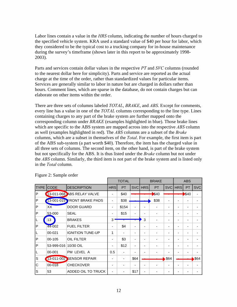