Embed Size (px)
Citation preview
mathematics
Article
An Improved Slime Mould Algorithm for Demand Estimationof Urban Water Resources
Kanhua Yu *, Lili Liu and Zhe Chen
�����������������
Citation: Yu, K.; Liu, L.; Chen, Z. An
Improved Slime Mould Algorithm for
Demand Estimation of Urban Water
Resources. Mathematics 2021, 9, 1316.
https://doi.org/10.3390/math9121316
Academic Editors: Daniel
Gómez Gonzalez, Javier Montero
and Tinguaro Rodriguez
Received: 10 May 2021
Accepted: 2 June 2021
Published: 8 June 2021
Publisher’s Note: MDPI stays neutral
with regard to jurisdictional claims in
published maps and institutional affil-
iations.
Copyright: © 2021 by the authors.
Licensee MDPI, Basel, Switzerland.
This article is an open access article
distributed under the terms and
conditions of the Creative Commons
Attribution (CC BY) license (https://
creativecommons.org/licenses/by/
4.0/).
Department of Urban and Rural Planning, Academy of Architecture, Chang’an University, Xi’an 710061, China;[email protected] (L.L.); [email protected] (Z.C.)* Correspondence: [email protected]
Abstract: A slime mould algorithm (SMA) is a new meta-heuristic algorithm, which can be widelyused in practical engineering problems. In this paper, an improved slime mould algorithm (ESMA)is proposed to estimate the water demand of Nanchang City. Firstly, the opposition-based learningstrategy and elite chaotic searching strategy are used to improve the SMA. By comparing theESMA with other intelligent optimization algorithms in 23 benchmark test functions, it is verifiedthat the ESMA has the advantages of fast convergence, high convergence precision, and strongrobustness. Secondly, based on the data of historical water consumption and local economic structureof Nanchang, four estimation models, including linear, exponential, logarithmic, and hybrid, areestablished. The experiment takes the water consumption of Nanchang City from 2004 to 2019 asan example to analyze, and the estimation models are optimized using the ESMA to determinethe model parameters, then the estimation models are tested. The simulation results show thatall four models can obtain better prediction accuracy, and the proposed ESMA has the best effecton the hybrid prediction model, and the prediction accuracy is up to 97.705%. Finally, the waterconsumption of Nanchang in 2020–2024 is forecasted.
Keywords: water demand estimation; slime mould algorithm; opposition-based learning; elitechaotic searching strategy; parameters optimization
1. Introduction
Water is a very precious natural resource, even called the source of life. With thecontinuous economic development and population growth, people’s demand for water isalso increasing. However, due to the long regeneration cycle of water, the contradictionbetween the supply and demand of water resources is more and more tense, resulting ina serious shortage of water resources. Therefore, the optimal and reasonable allocationof water resources is the key to sustainable utilization of water resources [1]. Due to therandomness of water consumption and the influence of the economy, population, and otherfactors, water resources demand estimation has always been a very difficult problem.
At present, the methods of water resources prediction at home and abroad are var-ied [2]. From the spatial and temporal scale of the forecast, it can be divided into ashort-term, medium-term, long-term, global, national forecast, and so on. From the rangeof the forecast, it can be divided into the whole forecast and partial forecast. From theapproach of the forecast, it can be divided into grey correlation model [3], regressionanalysis model [4], and neural network prediction model [5]. Although the traditionalforecast models can predict the demand for water resources by different approaches, thelow predicted accuracy of those models might not apply to solving practical problems.Choosing the appropriate parameters in the models is an effective way to eliminate theeffect of sparsity and uncertainty of historical data, and improve the accuracy of predictedresults. The selection of parameters among so many candidates is a challenging task andcan be regarded as an optimization problem. Therefore, intelligent optimization algorithmsare used to solve such parametric optimization models. In order to effectively ameliorate
Mathematics 2021, 9, 1316. https://doi.org/10.3390/math9121316 https://www.mdpi.com/journal/mathematics
Mathematics 2021, 9, 1316 2 of 26
the demand estimation of irrigation water, Pulido-Calvo and Gutiérrez-Estrada studieda hybrid model based on genetic algorithm and computational neural network, as wellas fuzzy logic in [6]. Bai et al. [7] proposed a multi-scale urban water resources demandestimation method based on an adaptive chaotic particle swarm optimization algorithmto search weight factors. Romano and Kapelan [8] constructed a valid estimation modelwith an average error of about 5% using evolutionary algorithms and artificial neuralnetworks. Similarly, Oliveira et al. [9] applied the harmonious search algorithm to theshort-term water demand estimation and searched the parameters in the model by us-ing the harmony search (HS) algorithm. Swarm intelligence optimization algorithms areresearch hotspots in the optimization field. Swarm intelligence optimization algorithmssimulate biological, social behavior, among which the most classic algorithm is particleswarm optimization (PSO) [10]. In recent years, other swarm intelligence optimizationalgorithms proposed include whale optimization algorithm (WOA) [11], gray wolf op-timizer (GWO) [12], harris hawk optimization (HHO) [13], firefly algorithm (FA) [14],manta rays foraging optimization (MRFO) [15], marine predators algorithm (MPA) [16],slime mould algorithm (SMA) [17], etc. Among them, the SMA is a new meta-heuristicalgorithm proposed by Li et al. [17] in 2020, which is inspired by the diffusion and foragingbehavior of slime mould. The SMA algorithm has the advantages of strong global searchability and strong robustness, so it has been applied to solve some practical engineeringoptimization problems [18–26]. But at the same time, the SMA also has some defects, suchas low calculation accuracy and premature convergence on some benchmark functions. Inorder to improve the convergence accuracy and speed of the algorithm, a new, improvedslime mould algorithm (ESMA) is proposed. In view of the four water resources estimationmodels (linear, logarithmic, exponential, and hybrid) established in Nanchang City, theESMA is used to optimize the model parameters and test the models. In addition, theESMA is compared with other intelligent algorithms in the models, and the future waterconsumption of Nanchang City in 2020–2024 is predicted.
The rest of this paper is organized as follows: In Section 2, an improved slime mouldalgorithm (ESMA) is proposed. In Section 3, the ESMA is compared with the other sixoptimization algorithms on 23 test functions, and the superiority of the ESMA is verified byexperiments. In Section 4, four estimation models of linear, logarithmic, exponential, andhybrid are proposed to predict the water resources of Nanchang City. The ESMA is used tooptimize the model parameters, and the models are tested, and the simulation results anddiscussion are given. Finally, the work is summarized in Section 5.
2. An Improved Slime Mould Algorithm2.1. Slime Mould Algorithm
The slime mould algorithm (SMA) was proposed by Li et al. [17] in 2020, which wasinspired by the diffusion and foraging behavior of slime mould in nature. In this paper,the “slime mould” refers to Physarum polycephalum, and the main study in this paper isthe nutritional stage of the slime mould, in which the organic matter in the slime mould isresponsible for finding, surrounding, and digesting food. The mathematical models forthese stages are shown below.
2.1.1. Initialization
A single objective optimization model can be represented by Equation (1),
min f (X)s.t. lb ≤ X ≤ ub
(1)
where f (x) is the optimization function, and lb, ub ∈ Rd are the lower and upper bound ofthe variable x ∈ Rd
Mathematics 2021, 9, 1316 3 of 26
For the above d-dimensional optimization problem, the initial slime mould populationwith n individuals is a n × d matrix called X(0) = {X1, X2, · · · , Xn},. Each individual inthe population is a vector with d elements, which is initialized by Equation (2).
Xi = lb + rand·(ub− lb), i = 1, 2, . . . , n (2)
2.1.2. Approach Food
Since slime mould can approach food according to the smell in the air, and thisapproach behavior can be expressed by the following formula,
X(t + 1){
Xb(t) + vb·(W·XA(t)− XB(t)), r < pvc·X(t), r ≥ p
(3)
where, t represents the current iteration number, X represents the position of slime mould,Xb is the individual position with the highest odor concentration, XA and XB are the twoindividuals randomly selected from the population. The selection behavior of slime mouldis simulated by two parameters, vb and vc, and the value range of vb is [−a, a], vc decreasedlinearly from 1 to 0. r is a random number between [0, 1], W represents the weight of thesearch agent.
The formula of p is expressed as follows,
p = tanh|S(i)− DF|, i = 1, 2, . . . , n (4)
where, S(i) represents the fitness value of the current individual, and DF represents theoptimal fitness value in all the current iterations.
The expression of vb is as follows,
vb = [−a, a], a = arctanh(− 2max_t
+ 1) (5)
where, max_t represents the maximum number of iterations.The weight W is given as follows,
W(SmellIndex(i) =
1 + r· log(
bF−S(i)bF−wF + 1
), condition
1 + r· log( bF−S(i)bF−wF + 1
), others
(6)
SmellIndex = sort(S) (7)
where, r is a random number between [0, 1], condition represents the first half of thepopulation. bF and wF, respectively, represent the optimal and worst value obtained in thecurrent iteration, and SmellIndex denotes the sequence of fitness values sorted (ascends inthe minimum value problem).
2.1.3. Wrap Food
This stage simulates the contraction mode of venous tissue structure of slime mouldmathematically when searching. The slime mould can adjust its search patterns accordingto the quality of food. The specific mathematical formula of the slime mould updating itsposition can be expressed as
X∗ =
rand·(ub− lb) + lb, rand < z
Xb(t) + vb·(W·XA(t)− XB(t)), r < pvc·X(t), r ≥ p
(8)
where, ub and lb are the upper and lower bounds of the search space, respectively, randand r are random numbers between [0, 1]. z is a parameter of balancing algorithm’s
Mathematics 2021, 9, 1316 4 of 26
exploration and exploitation capability, and different values can be selected according tospecific problems. In this paper, z is 0.03.
Algorithm 1 gives the pseudo-code of the SMA.
Algorithm 1. Slime mould algorithm
Input: Slime mould population Xi (i = 1,2, . . . ,n) and related parameters such as n, dim, max_t;Output: Optimal fitness value best_fitness and the corresponding optimal position Xb.While (t < max_t)
Check if solutions go outside the search space and bring them backCalculate fitness values of all individuals, update the best and worst fitness valueCalculate the weight W according to Equation (6)Record the best fitness best_fitness and the corresponding XbFor each search agent
Update the value of vb, vc, and pUpdate the individual position according to Equation (8)
End Fort = t + 1
End While
2.2. The Proposed Improved Slime Mould Algorithm2.2.1. Opposition-Based Learning
According to the idea of opposition-based learning (OBL) [27,28], in the optimizationprocess, the current solution has a 50% probability of being far away from the optimal solu-tion of the problem compared with its opposition solution. Therefore, selecting the betterindividual from the current solution population and the opposition solution population asthe new generation population can accelerate the convergence to a certain extent, increasethe diversity of the population, and improve the performance of the algorithm.
Suppose that the size of the population is n, then the population is represented asX = (X1, X2, · · · , Xn)′, ub and lb represent the upper and lower bounds of the search agent,respectively. Let the algorithm generates n opposite solutions through the opposition-basedlearning, then the opposite population can be represented as X̃ = (X̃1, X̃2, · · · , X̃n)′, thespecific calculation formula of opposition-based learning is
X̃i = lb + ub− Xi (9)
The fitness values of the current solution population X and the opposition solutionpopulation X̃ were calculated, respectively. Among the 2n individuals composed of thecurrent solution population and the opposition solution population, that is X2n = {Xi, i =1, · · · , n} ∪ {X̃i, i = 1, · · · , n}, n individuals with better fitness values were selected as thenew generation population.
2.2.2. Elite Chaotic Searching Strategy
Opposition-based learning strategy mainly emphasizes the exploration ability ofthe algorithm, and to improve the exploitation ability of the algorithm, an elite chaoticsearching strategy is added. Through chaotic mutation of the elite individual, the algorithmcan further update the elite individual, this can improve the exploitation ability of thealgorithm. The specific update process for the elite chaotic searching strategy is as follows.
Firstly, the fitness value of all the individuals (n) in the current population are cal-culated and sorted, and the first m(m = pr · n) individuals with better fitness value areselected as the elite individuals of the current population, where pr ∈ [0, 1] is the se-lected elite proportion, and pr = 0.1 in this paper. The selected elite individuals aredenoted as {EX1(t), EX2(t), · · · , EXm(t)}∈ {X1(t), X2(t), · · · , Xn(t)} and the upper andlower bounds of the j-th dimension are respectively:{
Ebj(t) = max(EX1j(t), EX2j(t), · · · , EXmj(t))Eaj(t) = min(EX1j(t), EX2j(t), · · · , EXmj(t))
(10)
Mathematics 2021, 9, 1316 5 of 26
Then, the elite individuals are mapped from the search space to the interval [0, 1]according to Equation (11), and the chaotic individuals Ci(t) = (Ci1(t), Ci2(t), · · · , Cid(t))are obtained, where d is the dimension of individuals.
Ci(t) =EXi(t)− lb
ub− lb, i = 1, 2, · · · , m (11)
Logistic chaotic mapping is iterated for Cij(t) according to the following equation
Ck+1ij (t) = µ · Ck
ij(t) · (1− Ckij(t)) (12)
where, i = 1, · · · , m; j = 1, · · · , d, constant µ = 4, k represents the number of chaoticiterations, and kmax is the maximum number of chaotic iterations. In this paper, themaximum number of current population iterations is taken as the maximum number ofchaotic iterations.
When the chaotic iteration reaches kmax, the chaotic individual Ckmaxij (t) are mapped
to [Eaj(t), Ebj(t)] according to the following formula to get the i-th new elite individualECij(t).
ECij(t) = Ckmaxij (t) · (Ebj(t)− Eaj(t)) + Eaj(t) (13)
Finally, a greedy selection is made between the elite individuals ECi(t) and EXi(t),and the individuals with better fitness value are selected to enter the next generation, i.e.,
EXi(t) ={
EXi(t) f (EXi(t)) ≤ f (ECi(t))ECi(t) f (EXi(t)) > f (ECi(t))
(14)
Due to the introduction of chaotic mutation in the strategy, the randomness of theposition of the elite individuals is enhanced, and the local search ability of the algorithmis improved accordingly. The greedy selection of the elite individuals can accelerate theconvergence speed of the algorithm. Experiments show that this strategy can improve theexploitation ability of the original algorithm.
2.2.3. The Improved Slime Mould Algorithm Combining the Two Strategies
This paper improves the original slime mould algorithm by adding opposition-basedlearning and an elite chaotic searching strategy into the SMA. The opposition-based learn-ing increases the population diversity, while the elite chaotic searching strategy improvesthe exploitation ability of the algorithm. The proposed improved slime mould algorithm iscalled the ESMA for short. The concrete steps of the improved algorithm are given below.
Step1: Initialize some parameters related to the ESMA, such as population size n,variable dimension dim, upper and lower bounds of variables, maximum iteration timesmax_t, etc.;
Step2: Initialize the population randomly by Equation (2), calculate the oppositionsolution population of the current population according to Equation (9), and sort the fitnessof the current solution population and the opposition solution population, and select thefirst n individuals with better fitness value as the current solution population;
Step3: When t < max_t, the fitness value of each individual is calculated, the best andthe worst fitness values are updated;
Step4: Update the value of weight W with Equation (6), update the minimum fitnessvalue as the optimal value best_fitness, and record the optimal individual Xb correspondingto the optimal value;
Step5: Update parameters p, vb, and vc for each individual, and update populationposition according to Equation (8);
Step6: Perform opposition-based learning operation for the current population accordingto Equation (9), then sort the fitness of the current solution population and the opposition
Mathematics 2021, 9, 1316 6 of 26
solution population, select the first n individuals with better fitness value as the currentpopulation, and then execute elite chaotic searching strategy according to Equations (10)–(14);
Step7: Let t = t + 1, if t < max_t, returns Step3, otherwise, outputs the optimal valuebest_fitness and the optimal individual Xb.
In addition, Algorithm 2 gives the pseudo-code of the ESMA.
Algorithm 2. Pseudo-code of the ESMA
Initialize related parameters such as n, dim, max_t, and Slime mould population Xi (i = 1,2,...,n);Calculate opposition population X̃ of current population Xi (i = 1,2, . . . ,n) by Equation (9)Calculate the fitness of population X̃ ∪ X, pick n individuals with better fitness value as thecurrent populationWhile (t < max_t)
Calculate fitness values of all individuals, update the best and worst fitness valueCalculate the weight W according to Equation (6)Record the best fitness best_fitness and the corresponding XbFor i = 1: n
Update the value of vb, vc, and pUpdate the population position according to Equation (8)
End ForCalculate X̃ by Equation (9), pick n individuals with better fitness value as the current
population based on the fitness values of population X̃ ∪ XSelect the first m individuals as elite individuals EXiCalculate new elite individuals obtained by chaotic iteration through Equations (10)–(13)Update the elite individuals’ position according to Equation (14)Check if solutions go outside the search space and bring them backt = t + 1
End WhileReturn optimal fitness value best_fitness and the corresponding optimal position Xb
3. Comparison of the ESMA with Other Algorithms
In order to further test the performance of the ESMA, it is compared with otherintelligent algorithms. In this section, the ESMA is compared with other six algorithmsin twenty-three test functions, and the six algorithms are the GWO [12], WOA [11], antlion optimizer (ALO) [29], sine cosine algorithm (SCA) [30], moth-flame optimization(MFO) [31], and the original the SMA [17], the parameters setting in the Algorithms areshown in Table 1. To get unbiased experimental result, all the experiments are carried outon the same computer, and the detailed settings are shown in Table 2. Tables 3–5 show23 benchmark test functions—they can effectively evaluate the ability of algorithms toexplore, exploit and avoid falling into local optimum. Table 3 is unimodal test functions—itis mainly used to evaluate the exploitation ability of the algorithm. Table 4 is multimodaltest functions—it can test the exploration performance of the algorithm, and the fixed-dimensional multimodal test functions in Table 5 can test the ability of the algorithm tojump out of local extremums in low dimensions.
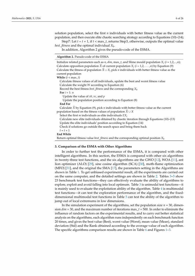
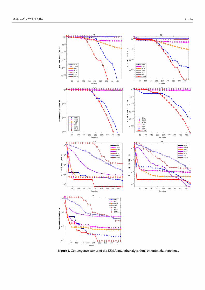
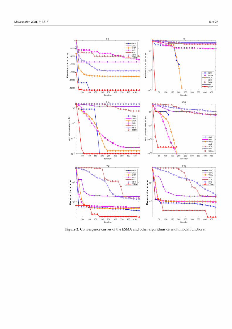
In the simulation experiment of the algorithms, set the population size n = 30, dimen-sion dim = 30, and the maximum number of iterations max_t = 500. In order to eliminate theinfluence of random factors on the experimental results, and to carry out better statisticalanalysis on the algorithms, each algorithm runs independently on each benchmark function20 times, and gives the best value (Best), worst value (Worst), mean value (Mean), standarddeviation (Std) and the Rank obtained according to the average value of each algorithm.The specific algorithms comparison results are shown in Table 6 and Figures 1–3.
Mathematics 2021, 9, 1316 7 of 26
Mathematics 2021, 9, x FOR PEER REVIEW 12 of 27
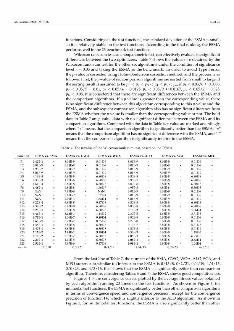
F18 1.48E-1 = 6.80E-8 - 6.80E-8 - 9.13E-7 - 6.80E-8 - 5.71E-8 + F19 1.40E-1 = 6.80E-8 - 6.80E-8 - 6.80E-8 + 6.80E-8 - 8.01E-9 + F20 3.15E-2 = 5.61E-1 = 5.98E-1 = 6.56E-3 + 6.80E-8 - 1.29E-3 - F21 8.10E-2 = 7.95E-7 - 6.80E-8 - 2.85E-1 = 6.80E-8 - 6.93E-3 - F22 2.29E-1 = 1.10E-5 - 6.80E-8 - 1.08E-1 = 6.80E-8 - 2.83E-1 = F23 2.50E-1 = 5.87E-6 - 9.17E-8 - 5.98E-1 = 6.80E-8 - 1.04E-1 = +/=/- 0/15/8 0/2/21 0/4/19 4/4/15 0/0/23 4/3/16
From the last line of Table 7, the number of the SMA, GWO, WOA, ALO, SCA, and MFO superior to/similar to/inferior to the ESMA is 0/15/8, 0/2/21, 0/4/19, 4/4/15, 0/0/23, and 4/3/16, this shows that the ESMA is significantly better than comparison algorithm. Therefore, considering Tables 6 and 7, the ESMA shows good competitiveness.
50 100 150 200 250 300 350 400 450Iteration
10-250
10-200
10-150
10-100
10-50
100F1
SMAGWOWOAALOSCAMFOESMA
50 100 150 200 250 300 350 400 450Iteration
10-150
10-100
10-50
100
F2
SMAGWOWOAALOSCAMFOESMA
50 100 150 200 250 300 350 400 45010-300
10-200
10-100
100F3
Iteration
SMAGWOWOAALOSCAMFOESMA
50 100 150 200 250 300 350 400 450Iteration
10-250
10-200
10-150
10-100
10-50
100F4
SMAGWOWOAALOSCAMFOESMA
50 100 150 200 250 300 350 400 450Iteration
100
102
104
106
108
F5
SMAGWOWOAALOSCAMFOESMA
50 100 150 200 250 300 350 400 450Iteration
10-2
100
102
104
F6
SMAGWOWOAALOSCAMFOESMA
Mathematics 2021, 9, x FOR PEER REVIEW 13 of 27
Figure 1. Convergence curves of the ESMA and other algorithms on unimodal functions.
Figure 2. Convergence curves of the ESMA and other algorithms on multimodal functions.
50 100 150 200 250 300 350 400 450Iteration
10-4
10-2
100
102F7
SMAGWOWOAALOSCAMFOESMA
50 100 150 200 250 300 350 400 450Iteration
-12000
-10000
-8000
-6000
-4000
-2000
0F8
SMAGWOWOAALOSCAMFOESMA
50 100 150 200 250 300 350 400 450Iteration
10-10
10-5
100
F9
SMAGWOWOAALOSCAMFOESMA
50 100 150 200 250 300 350 400 450Iteration
10-15
10-10
10-5
100
F10
SMAGWOWOAALOSCAMFOESMA
50 100 150 200 250 300 350 400 450Iteration
10-15
10-10
10-5
100
F11
SMAGWOWOAALOSCAMFOESMA
50 100 150 200 250 300 350 400 450Iteration
100
105
F12
SMAGWOWOAALOSCAMFOESMA
50 100 150 200 250 300 350 400 450Iteration
100
105
F13
SMAGWOWOAALOSCAMFOESMA
Figure 1. Convergence curves of the ESMA and other algorithms on unimodal functions.
Mathematics 2021, 9, 1316 8 of 26
Mathematics 2021, 9, x FOR PEER REVIEW 13 of 27
Figure 1. Convergence curves of the ESMA and other algorithms on unimodal functions.
Figure 2. Convergence curves of the ESMA and other algorithms on multimodal functions.
50 100 150 200 250 300 350 400 450Iteration
10-4
10-2
100
102F7
SMAGWOWOAALOSCAMFOESMA
50 100 150 200 250 300 350 400 450Iteration
-12000
-10000
-8000
-6000
-4000
-2000
0F8
SMAGWOWOAALOSCAMFOESMA
50 100 150 200 250 300 350 400 450Iteration
10-10
10-5
100
F9
SMAGWOWOAALOSCAMFOESMA
50 100 150 200 250 300 350 400 450Iteration
10-15
10-10
10-5
100
F10
SMAGWOWOAALOSCAMFOESMA
50 100 150 200 250 300 350 400 450Iteration
10-15
10-10
10-5
100
F11
SMAGWOWOAALOSCAMFOESMA
50 100 150 200 250 300 350 400 450Iteration
100
105
F12
SMAGWOWOAALOSCAMFOESMA
50 100 150 200 250 300 350 400 450Iteration
100
105
F13
SMAGWOWOAALOSCAMFOESMA
Figure 2. Convergence curves of the ESMA and other algorithms on multimodal functions.
Mathematics 2021, 9, 1316 9 of 26Mathematics 2021, 9, x FOR PEER REVIEW 14 of 27
50 100 150 200 250 300 350 400 450Iteration
100
101
102
F14
SMAGWOWOAALOSCAMFOESMA
50 100 150 200 250 300 350 400 450Iteration
10-3
10-2
10-1
100F15
SMAGWOWOAALOSCAMFOESMA
50 100 150 200 250 300 350 400 450Iteration
-1
-0.5
0
0.5
1
1.5
2
2.5
F16
SMAGWOWOAALOSCAMFOESMA
50 100 150 200 250 300 350 400 450Iteration
0.4
0.6
0.8
1
1.2
1.4
1.6
F17
SMAGWOWOAALOSCAMFOESMA
50 100 150 200 250 300 350 400 450Iteration
101
F18
SMAGWOWOAALOSCAMFOESMA
50 100 150 200 250 300 350 400 450Iteration
-3.5
-3
-2.5
-2
-1.5
-1
-0.5
0F19
SMAGWOWOAALOSCAMFOESMA
50 100 150 200 250 300 350 400 450Iteration
-3
-2.5
-2
-1.5
-1
-0.5
0F20
SMAGWOWOAALOSCAMFOESMA
50 100 150 200 250 300 350 400 450Iteration
-10
-9
-8
-7
-6
-5
-4
-3
-2
-1
0F21
SMAGWOWOAALOSCAMFOESMA
Figure 3. Cont.
Mathematics 2021, 9, 1316 10 of 26Mathematics 2021, 9, x FOR PEER REVIEW 15 of 27
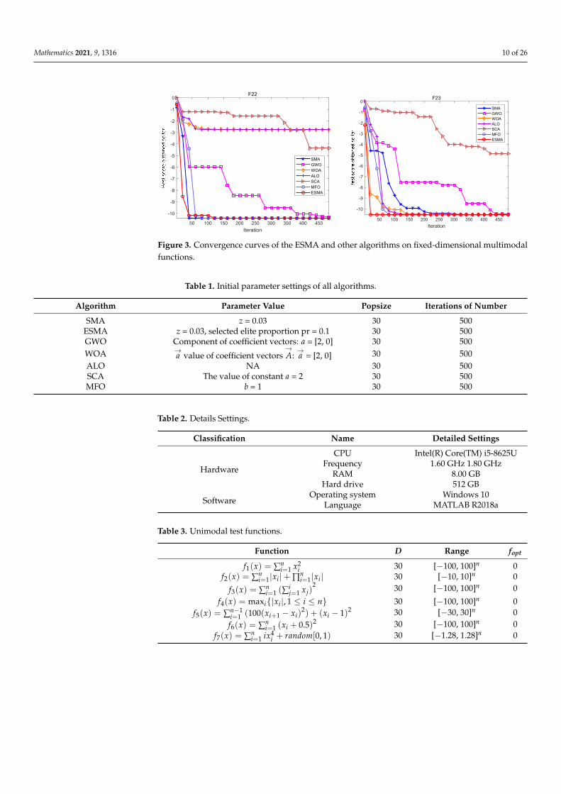
Figure 3. Convergence curves of the ESMA and other algorithms on fixed-dimensional multimodal functions.
Figures 1–3 are convergence curves plotted by the average fitness values obtained by each algorithm running 20 times on the test functions. As shown in Figure 1, for unimodal test functions, the ESMA is significantly better than other comparison algorithms in terms of convergence speed and convergence precision, except for the convergence precision of function F6, which is slightly inferior to the ALO algorithm. As shown in Figure 2, for multimodal test functions, the ESMA is also significantly better than other comparison algorithms in terms of convergence speed and convergence precision, and has good com-petitiveness. As shown in Figure 3, for the low-dimensional multimodal test functions, in the test function F16–F19, the difference between the seven algorithms is small, and they are basically close to the optimal value of the test function. For function F20, the ESMA is slightly inferior to the WOA and GWO in terms of convergence accuracy, while for other low-dimensional multimodal test functions, the ESMA performs better in terms of con-vergence speed and accuracy. In general, through the test of convergence curves, the pro-posed ESMA has obvious improvement in the convergence characteristics on the CEC-2005 benchmark functions.
4. The ESMA for Demand Estimation of Water Resources 4.1. Establishment of Water Resources Demand Estimation Model
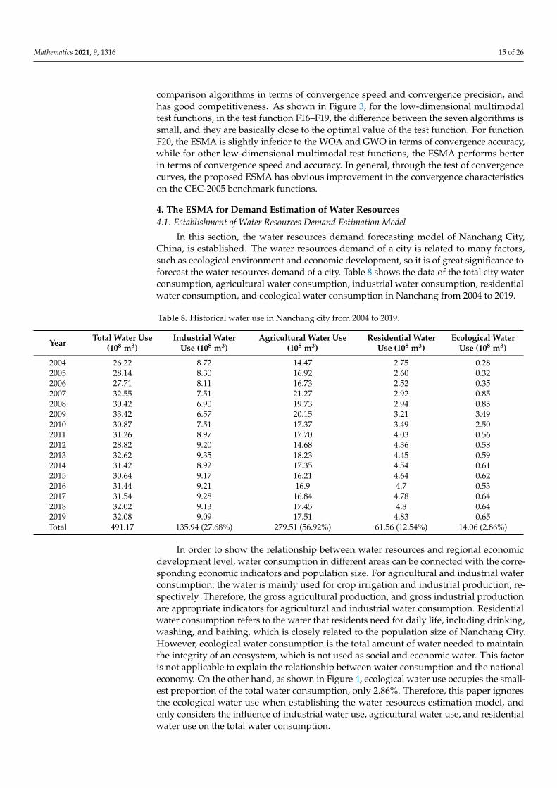
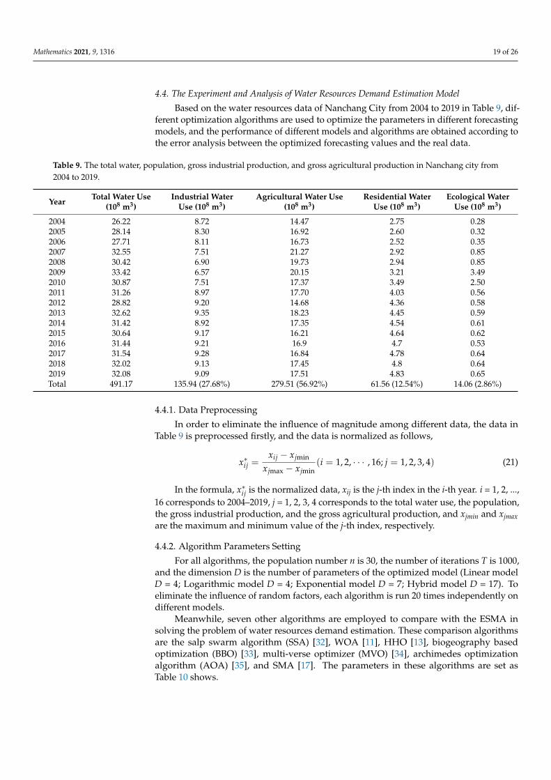
In this section, the water resources demand forecasting model of Nanchang City, China, is established. The water resources demand of a city is related to many factors, such as ecological environment and economic development, so it is of great significance to forecast the water resources demand of a city. Table 8 shows the data of the total city water consumption, agricultural water consumption, industrial water consumption, resi-dential water consumption, and ecological water consumption in Nanchang from 2004 to 2019.
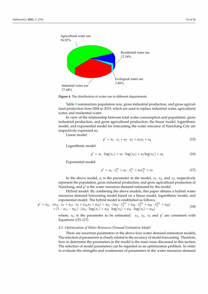
In order to show the relationship between water resources and regional economic development level, water consumption in different areas can be connected with the cor-responding economic indicators and population size. For agricultural and industrial wa-ter consumption, the water is mainly used for crop irrigation and industrial production, respectively. Therefore, the gross agricultural production, and gross industrial production are appropriate indicators for agricultural and industrial water consumption. Residential water consumption refers to the water that residents need for daily life, including drink-ing, washing, and bathing, which is closely related to the population size of Nanchang City. However, ecological water consumption is the total amount of water needed to maintain the integrity of an ecosystem, which is not used as social and economic water. This factor is not applicable to explain the relationship between water consumption and the national economy. On the other hand, as shown in Figure 4, ecological water use oc-cupies the smallest proportion of the total water consumption, only 2.86%. Therefore, this
50 100 150 200 250 300 350 400 450Iteration
-10
-9
-8
-7
-6
-5
-4
-3
-2
-1
0F22
SMAGWOWOAALOSCAMFOESMA
50 100 150 200 250 300 350 400 450Iteration
-10
-9
-8
-7
-6
-5
-4
-3
-2
-1
0F23
SMAGWOWOAALOSCAMFOESMA
Figure 3. Convergence curves of the ESMA and other algorithms on fixed-dimensional multimodalfunctions.
Table 1. Initial parameter settings of all algorithms.
Algorithm Parameter Value Popsize Iterations of Number
SMA z = 0.03 30 500ESMA z = 0.03, selected elite proportion pr = 0.1 30 500GWO Component of coefficient vectors: a = [2, 0] 30 500WOA →
a value of coefficient vectors→A:→a = [2, 0] 30 500
ALO NA 30 500SCA The value of constant a = 2 30 500MFO b = 1 30 500
Table 2. Details Settings.
Classification Name Detailed Settings
Hardware
CPU Intel(R) Core(TM) i5-8625UFrequency 1.60 GHz 1.80 GHz
RAM 8.00 GBHard drive 512 GB
SoftwareOperating system Windows 10
Language MATLAB R2018a
Table 3. Unimodal test functions.
Function D Range fopt
f1(x) = ∑ni=1 x2
i 30 [−100, 100]n 0f2(x) = ∑n
i=1|xi|+ ∏ni=1|xi| 30 [−10, 10]n 0
f3(x) = ∑ni=1 (∑
ij=1 xj)
2 30 [−100, 100]n 0
f4(x) = maxi{|xi|, 1 ≤ i ≤ n} 30 [−100, 100]n 0f5(x) = ∑n−1
i=1 (100(xi+1 − xi)2) + (xi − 1)2 30 [−30, 30]n 0
f6(x) = ∑ni=1 (xi + 0.5)2 30 [−100, 100]n 0
f7(x) = ∑ni=1 ix4
i + random[0, 1) 30 [−1.28, 1.28]n 0
Mathematics 2021, 9, 1316 11 of 26
Table 4. Multimodal test functions.
Function D Range fopt
f8(x) = ∑ni=1 (xi sin(
√|xi|)) 30 [−500, 500]n −12,569.5
f9(x) = ∑ni=1 (x2
i − 10 cos(2πxi) + 10)2 30 [−5.12, 5.12]n 0
f10(x) = −20 exp(−0.2√
1n ∑n
i=1 x2i )− exp( 1
n ∑ni=1 cos 2πxi) + 20 + e 30 [−32, 32]n 0
f11(x) = 14000 ∑n
i=1 (xi − 100)2 −∏ni=1 cos( xi−100√
i) + 1 30 [−600, 600]n 0
f12(x) = πn 10 sin 2(πy1) + ∑n−1
i=1 (yi − 1)2[1 + 10 sin 2(πyi + 1)]+(yn − 1)2 + ∑30
i=1 u(xi, 10, 100, 4)30 [−50, 50]n 0
f13(x) = 0.1 sin 2(3πx1) + ∑29i=1 (xi − 1)2 p[1 + sin 2(3πxi+1)]
+(xn − 1)2[1 + sin 2(2πx30)] + ∑30i=1 u(xi, 5, 10, 4)
30 [−50, 50]n 0
Table 5. Fixed-dimensional multimodal test functions.
Function D Range fopt
f14(x) =[
1500 + ∑25
j=11
j+∑2j=1 (xi−aij)
6
]−12 [−65.536, 65.536]n 0.998
f15(x) = ∑11i=1
∣∣∣ai −x1(b2
i +bi x2)
b2i +bi x3+x4
∣∣∣2 4 [−5, 5]n 3.075 × 10⁻⁴
f16(x) = 4x21 − 2.1x4
1 +13 x6
1 + x1x2 − 4x22 + 4x4
2 2 [−5, 5]n −1.0316
f17(x) = (x2 − 5.14π2 x2
1 +5π x1 − 6)
2+ 10(1− 1
8π ) cos x1 + 10 2 [−5, 5]n 0.398
f18(x) = [1 + (x1 + x2 + 1)2(19− 14x1 + 3x21 − 14x2 + 6x1x2 + 3x2
2)]
×[30 + (2x1 + 1− 3x2)2(18− 32x1 + 12x2
1 + 48x2 − 36x1x2 + 27x22)]
2 [−2, 2]n 3
f19(x) = −∑4i=1 exp[−∑3
j=1 aij(xj − pij)2] 3 [0, 1]n −3.86
f20(x) = −∑4i=1 exp[−∑6
j=1 aij(xj − pij)2] 6 [0, 1]n −3.322
f21(x) = −∑5i=1
∣∣∣(xi − ai)(xi − ai)T + ci
∣∣∣−1 4 [0, 10]n −10.1532
f22(x) = −∑7i=1
∣∣∣(xi − ai)(xi − ai)T + ci
∣∣∣−1 4 [0, 10]n −10.4028
f23(x) = −∑10i=1
∣∣∣(xi − ai)(xi − ai)T + ci
∣∣∣−1 4 [0, 10]n −10.5363
Table 6. Results of the ESMA and other optimization algorithms.
Algorithms
GWO WOA ALO SCA MFO SMA ESMA
F1
Best 4.31E-29 7.16E-82 2.00E-4 4.41E-3 7.01E-1 0 0Worst 6.38E-27 7.28E-75 5.01E-3 4.52E+1 2.00E+4 0 0Mean 1.48E-27 9.44E-76 1.57E-3 1.09E+1 3.03E+3 0 0
Std 2.01E-27 1.84E-75 1.21E-3 1.32E+1 5.70E+3 0 0Rank 3 2 4 5 6 1 1
F2
Best 3.37E-17 2.71E-55 2.3137 7.20E-6 4.07E-1 1.54E-284 0Worst 4.36E-16 3.54E-50 1.20E+2 6.19E-2 8.00E+1 3.58E-151 0Mean 1.31E-16 1.87E-51 4.73E+1 1.23E-2 3.04E+1 1.79E-152 0
Std 1.09E-16 7.88E-51 4.72E+1 1.78E-2 2.44E+1 8.04E-152 0Rank 4 3 7 5 6 2 1
F3
Best 2.84E-9 1.49E+4 1.22E+3 2.74E+3 1.72E+3 0 0Worst 5.78E-4 5.90E+4 9.89E+3 2.28E+4 5.39E+4 6.47E-295 0Mean 3.37E-5 3.75E+4 4.12E+3 9.45E+3 2.08E+4 3.24E-296 0
Std 1.28E-4 1.07E+4 2.03E+3 5.15E+3 1.25E+4 0 0Rank 3 7 4 5 6 2 1
F4
Best 9.21E-8 1.6832 7.3298 1.99E+1 5.56E+1 3.82E-288 0Worst 2.10E-6 8.93E+1 2.71E+1 5.30E+1 8.48E+1 4.17E-156 0Mean 6.73E-7 5.18E+1 1.68E+1 3.74E+1 6.76E+1 2.09E-157 0
Std 5.89E-7 2.81E+1 5.1065 9.5060 8.9481 9.33E-157 0Rank 3 6 4 5 7 2 1
Mathematics 2021, 9, 1316 12 of 26
Table 6. Cont.
Algorithms
GWO WOA ALO SCA MFO SMA ESMA
F5
Best 2.61E+1 2.77E+1 2.70E+1 1.00E+2 2.36E+1 4.30E-1 2.48E-2Worst 2.87E+1 2.88E+1 2.05E+3 1.10E+5 8.00E+7 2.83E+1 6.2473Mean 2.73E+1 2.82E+1 3.24E+2 1.69E+4 7.80E+6 8.8490 1.0764
Std 8.32E-1 1.61E-1 2.99E+5 7.23E+8 5.75E+14 1.30E+2 2.0468Rank 3 4 5 6 7 2 1
F6
Best 8.26E-5 1.19E-1 2.68E-4 4.9784 3.56E-1 1.64E-3 3.53E-4Worst 1.5139 1.0976 4.22E-3 1.68E+2 1.01E+4 2.08E-2 1.01E-2Mean 6.72E-1 3.68E-1 1.10E-3 1.96E+1 1.00E+3 6.67E-3 4.01E-3
Std 1.44E-1 6.18E-2 1.45E-6 1.32E+3 9.47E+6 1.59E-5 6.64E-6Rank 5 4 1 6 7 3 2
F7
Best 8.91E-4 2.37E-4 1.56E-1 1.36E-2 9.39E-2 1.01E-05 1.95E-6Worst 6.99E-3 4.02E-3 4.93E-1 1.8531 2.8949 6.07E-4 1.86E-4Mean 2.56E-3 1.54E-3 2.79E-1 1.98E-1 7.07E-1 2.23E-4 7.38E-5
Std 1.34E-3 1.14E-3 8.70E-2 3.97E-1 9.82E-1 1.46E-4 5.19E-5Rank 4 3 6 5 7 2 1
F8
Best −7729.0907 −12568.933 −7095.6123 −4391.8124 −9972.9113 −12,569.38 −12,569.49Worst −3476.3214 −8256.6973 −5417.6748 −3425.6876 −7105.0606 −12,568.52 −12,568.31Mean −5941.1712 −10,238.026 −5556.2584 −3851.2001 −8482.0979 −12,569.01 −12,569.11
Std 1.07E+6 2.91E+6 1.37E+5 8.53E+4 5.48E+5 5.59E-2 1.38E-1Rank 5 3 6 7 4 2 1
F9
Best 5.68E-14 0 4.38E+1 4.51E-1 1.04E+2 0 0Worst 1.44E+1 0 1.17E+2 1.06E+1 2.52E+2 0 0Mean 3.6616 0 7.91E+1 4.59E+1 1.62E+2 0 0
Std 4.1227 0 1.84E+1 2.84E+1 3.33E+1 0 0Rank 2 1 4 3 5 1 1
F10
Best 7.55E-14 8.88E-16 1.7783 1.41E-2 1.3811 8.88E-16 8.88E-16Worst 1.22E-13 7.99E-15 9.7666 2.04E+1 2.00E+1 8.88E-16 8.88E-16Mean 9.93E-14 3.91E-15 4.8695 1.52E+1 1.38E+1 8.88E-16 8.88E-16
Std 1.33E-14 3.11E-15 2.5083 8.5952 7.7738 0 0Rank 3 2 4 6 5 1 1
F11
Best 0 0 3.55E-3 4.36E-1 6.15E-1 0 0Worst 4.11E-2 1.10E-1 1.27E-1 1.3327 1.81E+2 0 0Mean 9.28E-3 7.82E-3 5.47E-2 8.52E-1 1.90E+1 0 0
Std 1.33E-2 2.62E-2 2.87E-2 2.60E-1 4.71E+1 0 0Rank 3 2 4 5 6 1 1
F12
Best 1.93E-2 8.79E-3 7.8128 1.2833 3.4831 4.07E-5 1.38E-6Worst 1.05E-1 4.51E-2 3.69E+1 1.28E+6 2.60E+1 1.51E-2 9.67E-3Mean 4.25E-2 2.13E-2 1.56E+1 6.44E+4 1.00E+1 4.91E-3 1.29E-3
Std 5.75E-4 1.18E-4 5.44E+1 8.25E+10 5.31E+1 2.23E-5 5.61E-6Rank 4 3 6 7 5 2 1
F13
Best 4.46E-1 5.88E-2 8.49E-2 3.0307 9.4540 4.91E-4 2.30E-5Worst 1.1132 1.1252 5.44E+1 2.25E+5 3.62E+2 7.06E-2 1.41E-2Mean 7.66E-1 4.68E-1 2.29E+1 1.24E+4 4.13E+1 1.14E-2 3.79E-3
Std 3.57E-2 8.03E-2 3.64E+2 2.50E+9 5.83E+3 2.64E-4 1.41E-5Rank 4 3 5 7 6 2 1
F14
Best 0.998 0.998 0.998 0.998 0.998 0.998 0.998Worst 12.6705 10.7632 6.9033 10.7632 7.874 0.998 0.998Mean 5.3046 3.7499 2.7291 2.0828 3.1201 0.998 0.998
Std 1.95E+1 1.11E+1 3.0575 5.0233 5.3292 7.86E-24 3.30E-25Rank 7 6 4 3 5 2 1
F15
Best 3.075E-4 3.078E-4 6.404E-4 4.884E-4 7.295E-4 3.075E-4 3.077E-4Worst 2.036E-2 2.194E-3 2.036E-2 1.535E-3 1.655E-3 1.227E-3 1.231E-3Mean 2.51E-3 8.72E-4 1.94E-3 9.78E-4 1.02E-3 5.93E-4 5.29E-4
Std 3.74E-5 3.46E-7 1.89E-5 1.27E-7 1.32E-7 1.25E-7 7.58E-8Rank 7 3 6 4 5 2 1
Mathematics 2021, 9, 1316 13 of 26
Table 6. Cont.
Algorithms
GWO WOA ALO SCA MFO SMA ESMA
F16
Best −1.0316 −1.0316 −1.0316 −1.0316 −1.0316 −1.0316 −1.0316Worst −1.0316 −1.0316 −1.0316 −1.0316 −1.0316 −1.0316 −1.0316Mean −1.0316 −1.0316 −1.0316 −1.0316 −1.0316 −1.0316 −1.0316
Std 5.53E-16 5.53E-19 5.94E-27 2.37E-9 5.19E-32 1.25E-18 3.97E-19Rank 6 4 2 7 1 5 3
F17
Best 0.39789 0.39789 0.39789 0.39789 0.39789 0.39789 0.39789Worst 0.39791 0.39792 0.39789 0.40907 0.39789 0.39789 0.39789Mean 0.39789 0.39789 0.39789 0.40037 0.39789 0.39789 0.39789
Std 2.62E-11 1.00E-10 1.17E-26 1.11E-5 0 9.22E-16 5.23E-16Rank 5 6 2 7 1 4 3
F18
Best 3 3 3 3 3 3 3Worst 3 3.0006 3 3.0004 3 3 3Mean 3 3.0001 3 3.0001 3 3 3
Std 1.66E-9 2.04E-8 6.35E-26 1.62E-8 7.71E-30 1.16E-20 1.84E-21Rank 5 7 4 6 1 3 2
F19
Best −3.8628 −3.8626 −3.8628 −3.8549 −3.8628 −3.8628 −3.8628Worst −3.8549 −3.8215 −3.8628 −3.8518 −3.8628 −3.8628 −3.8628Mean −3.8611 −3.852 −3.8628 −3.854 −3.8628 −3.8628 −3.8628
Std 7.17E-6 1.70E-4 3.18E-26 1.08E-6 5.19E-30 2.43E-13 6.37E-15Rank 5 7 2 6 1 4 3
F20
Best −3.322 −3.3216 −3.322 −3.1454 −3.322 −3.322 −3.322Worst −3.1365 −2.4512 −3.2018 −1.9187 −3.1327 −3.1974 −3.1997Mean −3.2502 −3.1889 −3.2683 −2.9488 −3.2347 −3.2559 −3.2142
Std 5.84E-3 4.05E-2 3.70E-3 7.15E-2 3.68E-3 3.76E-3 1.36E-3Rank 3 6 1 7 5 2 4
F21
Best −10.1528 −10.1502 −10.1532 −7.7535 −10.1532 −10.1532 −10.1532Worst −2.6826 −2.6271 −2.6305 −0.4982 −2.6305 −10.152 −10.1521Mean −7.632 −7.4809 −6.3745 −3.155 −5.1376 −10.1527 −10.1529
Std 8.6401 9.6374 1.09E+1 4.1255 9.8474 1.17E-7 1.30E-7Rank 3 4 5 7 6 2 1
F22
Best −10.4028 −10.4016 −10.4029 −6.555 −10.4029 −10.4029 −10.4029Worst −10.3969 −3.7181 −1.8376 −0.5239 −2.7519 −10.402 −10.4017Mean −10.4012 -8.197 −5.9837 −3.1307 −7.5086 −10.4025 −10.4026
Std 1.73E-6 7.6414 1.17E+1 3.37 1.35E+1 6.59E-8 9.85E-8Rank 3 4 6 7 5 2 1
F23
Best −10.5363 −10.5357 −10.5364 −6.7648 −10.5364 −10.5364 −10.5364Worst −2.4217 −2.4173 −1.6766 −0.94237 −2.8711 −10.5354 −10.5351Mean −9.8612 −7.3348 −7.2174 −3.6007 −8.1616 −10.5360 −10.5361
Std 4.4991 8.9562 1.47E+1 3.3493 1.12E+1 9.72E-8 8.31E-8Rank 3 5 6 7 4 2 1
Mean Rank 4.0435 4.1304 4.2609 5.7826 4.8261 2.2174 1.4783
Result 3 4 5 7 6 2 1
As shown in Table 6, for the unimodal test functions, namely, F1–F7, the ESMAcan accurately obtain the optimal value of the test functions on both F1–F4, showinggood optimization performance. The ESMA is slightly inferior to ALO on function F6,but obviously superior to it on other unimodal test functions. For the multimodal testfunctions, namely, F8–F13, the ESMA can also accurately obtain the optimal value of thetest functions on F9 and F11, and it is obviously better than other algorithms on othertest functions. For the low-dimensional multimodal test functions, the ESMA can alsoaccurately obtain the optimal value of the test functions on F14, F16, and F18, and theoptimization results of the seven algorithms on F16 and F18 are basically the same. Onfunction F16–F19, the mean value of the ESMA and MFO algorithm is the same, but thestandard deviation of the ESMA is slightly lower than that of the MFO algorithm. TheESMA is obviously better than other algorithms in other low dimensional multimodal test
Mathematics 2021, 9, 1316 14 of 26
functions. Considering all the test functions, the standard deviation of the ESMA is small,so it is relatively stable on the test functions. According to the final ranking, the ESMAperforms well in the 23 benchmark test functions.
Wilcoxon rank sum test, as a nonparametric test, can effectively evaluate the significantdifferences between the two optimizers. Table 7 shows the values of p obtained by theWilxocon rank sum test for the other six algorithms under the condition of significancelevel α = 0.05 and taking the ESMA as the benchmark. In order to avoid Type I error,the p-value is corrected using Holm–Bonferroni correction method, and the process is asfollows: First, the p-value of six comparison algorithms are sorted from small to large, ifthe sorting result is assumed to be p1 < p2 < p3 < p4 < p5 < p6, if p1 < 0.05/6 ≈ 0.0083,p2 < 0.05/5 = 0.01, p3 < 0.05/4 = 0.0125, p4 < 0.05/3 ≈ 0.0167, p5 < 0.05/2 = 0.025,p6 < 0.05, it is considered that there are significant differences between the ESMA andthe comparison algorithms. If a p-value is greater than the corresponding value, thereis no significant difference between this algorithm corresponding to this p-value and theESMA, and the subsequent comparison algorithm also has no significant difference fromthe ESMA whether the p-value is smaller than the corresponding value or not. The bolddata in Table 7 are p-value data with no significant difference between the ESMA and itscomparison algorithms. Combined with the data in Table 6, p-value are marked accordingly,where “+” means that the comparison algorithm is significantly better than the ESMA, “=“means that the comparison algorithm has no significant difference with the ESMA, and “-”means that the comparison algorithm is significantly inferior to the ESMA.
Table 7. The p-value of the Wilcoxon rank sum test, based on the ESMA.
Function ESMA vs. SMA ESMA vs. GWO ESMA vs. WOA ESMA vs. ALO ESMA vs. SCA ESMA vs. MFO
F1 3.42E-1 = 8.01E-9 - 8.01E-9 - 8.01E-9 - 8.01E-9 - 8.01E-9 -F2 8.01E-9 - 8.01E-9 - 8.01E-9 - 8.01E-9 - 8.01E-9 - 8.01E-9 -F3 1.98E-2 - 8.01E-9 - 8.01E-9 - 8.01E-9 - 8.01E-9 - 8.01E-9 -F4 8.01E-9 - 8.01E-9 - 8.01E-9 - 8.01E-9 - 8.01E-9 - 8.01E-9 -F5 4.16E-4 - 6.80E-8 - 6.80E-8 - 6.80E-8 - 6.80E-8 - 6.80E-8 -F6 8.35E-3 - 1.20E-6 - 6.80E-8 - 5.90E-5 - 6.80E-8 - 6.80E-8 -F7 1.61E-4 - 6.80E-8 - 6.80E-8 - 6.80E-8 - 6.80E-8 - 6.80E-8 -F8 1.48E-1 = 6.80E-8 - 1.66E-7 - 4.95E-8 - 6.80E-8 - 6.80E-8 -F9 NaN = 7.93E-9 - NaN = 8.01E-9 - 8.01E-9 - 8.01E-9 -
F10 NaN = 7.68E-9 - 1.57E-4 - 8.01E-9 - 8.01E-9 - 8.01E-9 -F11 NaN = 2.09E-3 - 1.63E-1 = 8.01E-9 - 8.01E-9 - 8.01E-9 -F12 6.22E-4 - 6.80E-8 - 9.17E-8 - 6.80E-8 - 6.80E-8 - 6.80E-8 -F13 4.39E-2 - 6.80E-8 - 6.80E-8 - 6.80E-8 - 6.80E-8 - 6.80E-8 -F14 9.25E-1 = 6.80E-8 - 6.80E-8 - 3.13E-2 = 6.80E-8 - 1.06E-1 =F15 9.46E-1 = 8.18E-1 = 1.44E-2 - 2.30E-5 - 4.68E-5 - 3.71E-5 -F16 6.75E-1 = 1.06E-7 - 9.89E-1 = 6.80E-8 + 6.80E-8 - 8.01E-9 +F17 9.68E-1 = 5.23E-7 - 8.35E-3 - 6.79E-8 + 6.80E-8 - 8.01E-9 +F18 1.48E-1 = 6.80E-8 - 6.80E-8 - 9.13E-7 - 6.80E-8 - 5.71E-8 +F19 1.40E-1 = 6.80E-8 - 6.80E-8 - 6.80E-8 + 6.80E-8 - 8.01E-9 +F20 3.15E-2 = 5.61E-1 = 5.98E-1 = 6.56E-3 + 6.80E-8 - 1.29E-3 -F21 8.10E-2 = 7.95E-7 - 6.80E-8 - 2.85E-1 = 6.80E-8 - 6.93E-3 -F22 2.29E-1 = 1.10E-5 - 6.80E-8 - 1.08E-1 = 6.80E-8 - 2.83E-1 =F23 2.50E-1 = 5.87E-6 - 9.17E-8 - 5.98E-1 = 6.80E-8 - 1.04E-1 =
+/=/- 0/15/8 0/2/21 0/4/19 4/4/15 0/0/23 4/3/16
From the last line of Table 7, the number of the SMA, GWO, WOA, ALO, SCA, andMFO superior to/similar to/inferior to the ESMA is 0/15/8, 0/2/21, 0/4/19, 4/4/15,0/0/23, and 4/3/16, this shows that the ESMA is significantly better than comparisonalgorithm. Therefore, considering Tables 6 and 7, the ESMA shows good competitiveness.
Figures 1–3 are convergence curves plotted by the average fitness values obtainedby each algorithm running 20 times on the test functions. As shown in Figure 1, forunimodal test functions, the ESMA is significantly better than other comparison algorithmsin terms of convergence speed and convergence precision, except for the convergenceprecision of function F6, which is slightly inferior to the ALO algorithm. As shown inFigure 2, for multimodal test functions, the ESMA is also significantly better than other
Mathematics 2021, 9, 1316 15 of 26
comparison algorithms in terms of convergence speed and convergence precision, andhas good competitiveness. As shown in Figure 3, for the low-dimensional multimodaltest functions, in the test function F16–F19, the difference between the seven algorithms issmall, and they are basically close to the optimal value of the test function. For functionF20, the ESMA is slightly inferior to the WOA and GWO in terms of convergence accuracy,while for other low-dimensional multimodal test functions, the ESMA performs betterin terms of convergence speed and accuracy. In general, through the test of convergencecurves, the proposed ESMA has obvious improvement in the convergence characteristicson the CEC-2005 benchmark functions.
4. The ESMA for Demand Estimation of Water Resources4.1. Establishment of Water Resources Demand Estimation Model
In this section, the water resources demand forecasting model of Nanchang City,China, is established. The water resources demand of a city is related to many factors,such as ecological environment and economic development, so it is of great significance toforecast the water resources demand of a city. Table 8 shows the data of the total city waterconsumption, agricultural water consumption, industrial water consumption, residentialwater consumption, and ecological water consumption in Nanchang from 2004 to 2019.
Table 8. Historical water use in Nanchang city from 2004 to 2019.
Year Total Water Use(108 m3)
Industrial WaterUse (108 m3)
Agricultural Water Use(108 m3)
Residential WaterUse (108 m3)
Ecological WaterUse (108 m3)
2004 26.22 8.72 14.47 2.75 0.282005 28.14 8.30 16.92 2.60 0.322006 27.71 8.11 16.73 2.52 0.352007 32.55 7.51 21.27 2.92 0.852008 30.42 6.90 19.73 2.94 0.852009 33.42 6.57 20.15 3.21 3.492010 30.87 7.51 17.37 3.49 2.502011 31.26 8.97 17.70 4.03 0.562012 28.82 9.20 14.68 4.36 0.582013 32.62 9.35 18.23 4.45 0.592014 31.42 8.92 17.35 4.54 0.612015 30.64 9.17 16.21 4.64 0.622016 31.44 9.21 16.9 4.7 0.532017 31.54 9.28 16.84 4.78 0.642018 32.02 9.13 17.45 4.8 0.642019 32.08 9.09 17.51 4.83 0.65Total 491.17 135.94 (27.68%) 279.51 (56.92%) 61.56 (12.54%) 14.06 (2.86%)
In order to show the relationship between water resources and regional economicdevelopment level, water consumption in different areas can be connected with the corre-sponding economic indicators and population size. For agricultural and industrial waterconsumption, the water is mainly used for crop irrigation and industrial production, re-spectively. Therefore, the gross agricultural production, and gross industrial productionare appropriate indicators for agricultural and industrial water consumption. Residentialwater consumption refers to the water that residents need for daily life, including drinking,washing, and bathing, which is closely related to the population size of Nanchang City.However, ecological water consumption is the total amount of water needed to maintainthe integrity of an ecosystem, which is not used as social and economic water. This factoris not applicable to explain the relationship between water consumption and the nationaleconomy. On the other hand, as shown in Figure 4, ecological water use occupies the small-est proportion of the total water consumption, only 2.86%. Therefore, this paper ignoresthe ecological water use when establishing the water resources estimation model, andonly considers the influence of industrial water use, agricultural water use, and residentialwater use on the total water consumption.
Mathematics 2021, 9, 1316 16 of 26
Mathematics 2021, 9, x FOR PEER REVIEW 16 of 27
paper ignores the ecological water use when establishing the water resources estimation model, and only considers the influence of industrial water use, agricultural water use, and residential water use on the total water consumption.
Table 8 summarizes population size, gross industrial production, and gross agricul-tural production from 2004 to 2019, which are used to replace industrial water, agricul-tural water, and residential water.
Figure 4. The distribution of water use in different departments.
Table 8. Historical water use in Nanchang city from 2004 to 2019.
Year Total Water Use (108 m3) Industrial Water Use (108 m3) Agricultural Water Use (108 m3) Residential Water Use (108 m3) Ecological Water
Use (108 m3) 2004 26.22 8.72 14.47 2.75 0.28 2005 28.14 8.30 16.92 2.60 0.32 2006 27.71 8.11 16.73 2.52 0.35 2007 32.55 7.51 21.27 2.92 0.85 2008 30.42 6.90 19.73 2.94 0.85 2009 33.42 6.57 20.15 3.21 3.49 2010 30.87 7.51 17.37 3.49 2.50 2011 31.26 8.97 17.70 4.03 0.56 2012 28.82 9.20 14.68 4.36 0.58 2013 32.62 9.35 18.23 4.45 0.59 2014 31.42 8.92 17.35 4.54 0.61 2015 30.64 9.17 16.21 4.64 0.62 2016 31.44 9.21 16.9 4.7 0.53 2017 31.54 9.28 16.84 4.78 0.64 2018 32.02 9.13 17.45 4.8 0.64 2019 32.08 9.09 17.51 4.83 0.65 Total 491.17 135.94 (27.68%) 279.51 (56.92%) 61.56 (12.54%) 14.06 (2.86%)
In view of the relationship between total water consumption and population, gross industrial production, and gross agricultural production, the linear model, logarithmic model, and exponential model for forecasting the water resource of Nanchang City are respectively expressed as,
Linear model:
4332211 axaxaxay ++⋅+⋅=′ (15)
Logarithmic model:
4332211 )log()log()log( axaxaxay ++⋅+⋅=′ (16)
Ecological water use2.86%
Residential water use12.54%
Agricultural water use56.92%
Industrial water use27.68%
Figure 4. The distribution of water use in different departments.
Table 8 summarizes population size, gross industrial production, and gross agricul-tural production from 2004 to 2019, which are used to replace industrial water, agriculturalwater, and residential water.
In view of the relationship between total water consumption and population, grossindustrial production, and gross agricultural production, the linear model, logarithmicmodel, and exponential model for forecasting the water resource of Nanchang City arerespectively expressed as,
Linear model:y′ = a1 · x1 + a2 · x2 + a3x3 + a4 (15)
Logarithmic model:
y′ = a1 · log(x1) + a2 · log(x2) + a3 log(x3) + a4 (16)
Exponential model:
y′ = a1 · xa21 + a3 · xa4
1 + a5xa61 + a7 (17)
In the above model, ai is the parameter in the model, x1, x2, and x3, respectivelyrepresent the population, gross industrial production, and gross agricultural production ofNanchang, and y′ is the water resources demand estimated by the model.
Hybrid model: By combining the above models, this paper obtains a hybrid waterresources demand forecasting model based on a linear model, logarithmic model, andexponential model. The hybrid model is established as follows,
y′ = a11 · (a12 · x1 + a13 · x2 + a14x3 + a15) + a21 · (a22 · xa231 + a24 · xa25
2 + a26 · xa273 + a28)
+(1− a11 − a21) · (a31 · log(x1) + a32 · log(x2) + a33 · log(x3) + a34)(18)
where, aij is the parameter to be estimated. x1, x2, x3 and y′ are consistent withEquations (15)–(17).
4.2. Optimization of Water Resources Demand Estimation Model
There are uncertain parameters in the above four water demand estimation models.The selection of parameters is closely related to the accuracy of model forecasting. Therefore,how to determine the parameters in the model is the main issue discussed in this section.The selection of model parameters can be regarded as an optimization problem. In orderto evaluate the strengths and weaknesses of parameters in the water resources demand
Mathematics 2021, 9, 1316 17 of 26
forecasting model, the sum of the squares of errors between the real value and the predictedvalue is used as the objective function, and its mathematical equation is as follows,
f (X) =k
∑i=1
(yi − y′ i)2 (19)
where, X is the parameter in the water resource demand forecasting model, k is the numberof years used in the optimization model, yi is the real total water consumption in the i-thyear, and y′ i is the estimated total water consumption in the i-th year. The smaller thevalue of the objective function is, the better the model parameters are, and the closer thepredicted value is to the real value. Therefore, the mathematical model of the optimizationproblem of water demand estimation model can be defined as,{
min f (X)s.t. l ≤ X ≤ u
(20)
where, X is the D-dimensional decision variable, D is the number of parameters in theestimation model, and u, l ∈ RD are the upper and lower bounds of parameters.
4.3. The ESMA Solves the Parameters of Water Demand Estimation Model
Section 4.2 establishes a specific mathematical model for solving water resourcesdemand parameters. The following shows the specific steps of solving the model with theESMA.
Step1: Initialize some parameters related to the ESMA, and take Equation (20) as theobjective function;
Step2: Initialize the population randomly, and perform the opposition-based learningoperation;
Step3: When t < max_t, the fitness value of each individual is calculated, the best andthe worst fitness values are updated;
Step4: Update the value of weight W with Equation (6), update the minimum fitnessvalue as the optimal value best_fitness, and record the optimal individual Xb correspondingto the optimal value;
Step5: Update parameters p, vb, and vc for each individual, and update populationposition according to Equation (8);
Step6: Perform opposition-based learning operation, and then execute elite chaoticsearching strategy;
Step7: Let t = t + 1, if t < max_t, returns Step3, otherwise, outputs the optimal valuebest_fitness and the optimal individual Xb.
Figure 5 shows the flow chart of the ESMA for solving water resources estimationparameters.
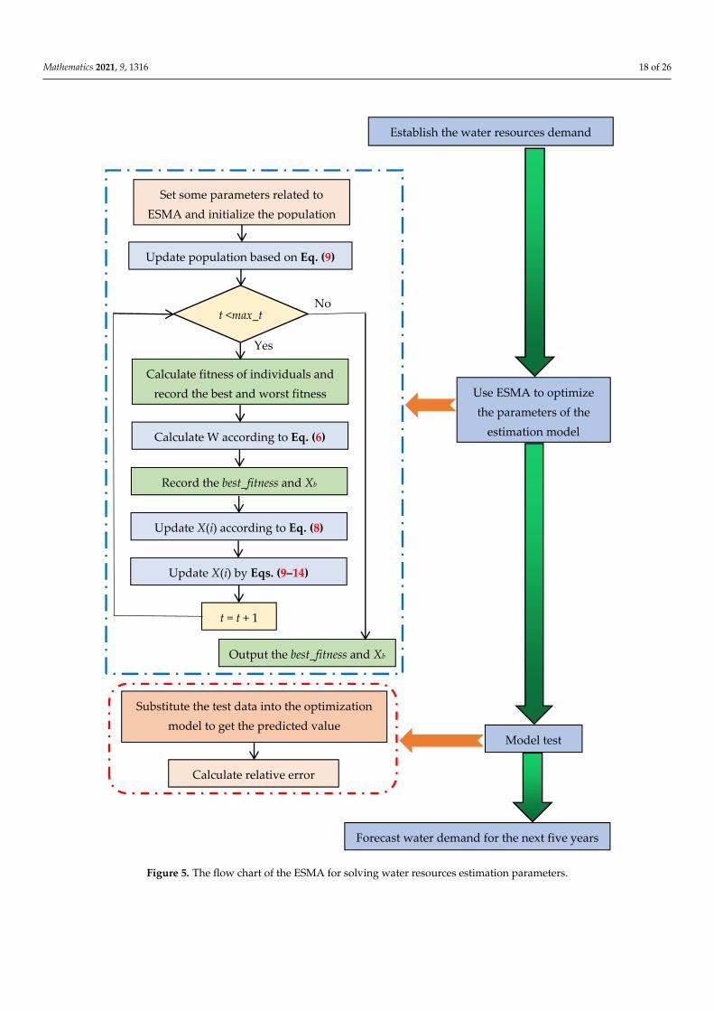
Mathematics 2021, 9, 1316 18 of 26Mathematics 2021, 9, x FOR PEER REVIEW 19 of 27
Figure 5. The flow chart of the ESMA for solving water resources estimation parameters.
Set some parameters related to ESMA and initialize the population
Update population based on Eq. (9)
Calculate fitness of individuals and record the best and worst fitness
Calculate W according to Eq. (6)
Record the best_fitness and Xb
t = t + 1
Update X(i) according to Eq. (8)
Use ESMA to optimize the parameters of the
estimation model
Model test
Update X(i) by Eqs. (9–14)
Forecast water demand for the next five years
Establish the water resources demand
t <max_t
Yes
No
Output the best_fitness and Xb
Substitute the test data into the optimization model to get the predicted value
Calculate relative error
Figure 5. The flow chart of the ESMA for solving water resources estimation parameters.
Mathematics 2021, 9, 1316 19 of 26
4.4. The Experiment and Analysis of Water Resources Demand Estimation Model
Based on the water resources data of Nanchang City from 2004 to 2019 in Table 9, dif-ferent optimization algorithms are used to optimize the parameters in different forecastingmodels, and the performance of different models and algorithms are obtained according tothe error analysis between the optimized forecasting values and the real data.
Table 9. The total water, population, gross industrial production, and gross agricultural production in Nanchang city from2004 to 2019.
Year Total Water Use(108 m3)
Industrial WaterUse (108 m3)
Agricultural Water Use(108 m3)
Residential WaterUse (108 m3)
Ecological WaterUse (108 m3)
2004 26.22 8.72 14.47 2.75 0.282005 28.14 8.30 16.92 2.60 0.322006 27.71 8.11 16.73 2.52 0.352007 32.55 7.51 21.27 2.92 0.852008 30.42 6.90 19.73 2.94 0.852009 33.42 6.57 20.15 3.21 3.492010 30.87 7.51 17.37 3.49 2.502011 31.26 8.97 17.70 4.03 0.562012 28.82 9.20 14.68 4.36 0.582013 32.62 9.35 18.23 4.45 0.592014 31.42 8.92 17.35 4.54 0.612015 30.64 9.17 16.21 4.64 0.622016 31.44 9.21 16.9 4.7 0.532017 31.54 9.28 16.84 4.78 0.642018 32.02 9.13 17.45 4.8 0.642019 32.08 9.09 17.51 4.83 0.65Total 491.17 135.94 (27.68%) 279.51 (56.92%) 61.56 (12.54%) 14.06 (2.86%)
4.4.1. Data Preprocessing
In order to eliminate the influence of magnitude among different data, the data inTable 9 is preprocessed firstly, and the data is normalized as follows,
x∗ij =xij − xjmin
xjmax − xjmin(i = 1, 2, · · · , 16; j = 1, 2, 3, 4) (21)
In the formula, x∗ij is the normalized data, xij is the j-th index in the i-th year. i = 1, 2, ...,16 corresponds to 2004–2019, j = 1, 2, 3, 4 corresponds to the total water use, the population,the gross industrial production, and the gross agricultural production, and xjmin and xjmaxare the maximum and minimum value of the j-th index, respectively.
4.4.2. Algorithm Parameters Setting
For all algorithms, the population number n is 30, the number of iterations T is 1000,and the dimension D is the number of parameters of the optimized model (Linear modelD = 4; Logarithmic model D = 4; Exponential model D = 7; Hybrid model D = 17). Toeliminate the influence of random factors, each algorithm is run 20 times independently ondifferent models.
Meanwhile, seven other algorithms are employed to compare with the ESMA insolving the problem of water resources demand estimation. These comparison algorithmsare the salp swarm algorithm (SSA) [32], WOA [11], HHO [13], biogeography basedoptimization (BBO) [33], multi-verse optimizer (MVO) [34], archimedes optimizationalgorithm (AOA) [35], and SMA [17]. The parameters in these algorithms are set asTable 10 shows.
Mathematics 2021, 9, 1316 20 of 26
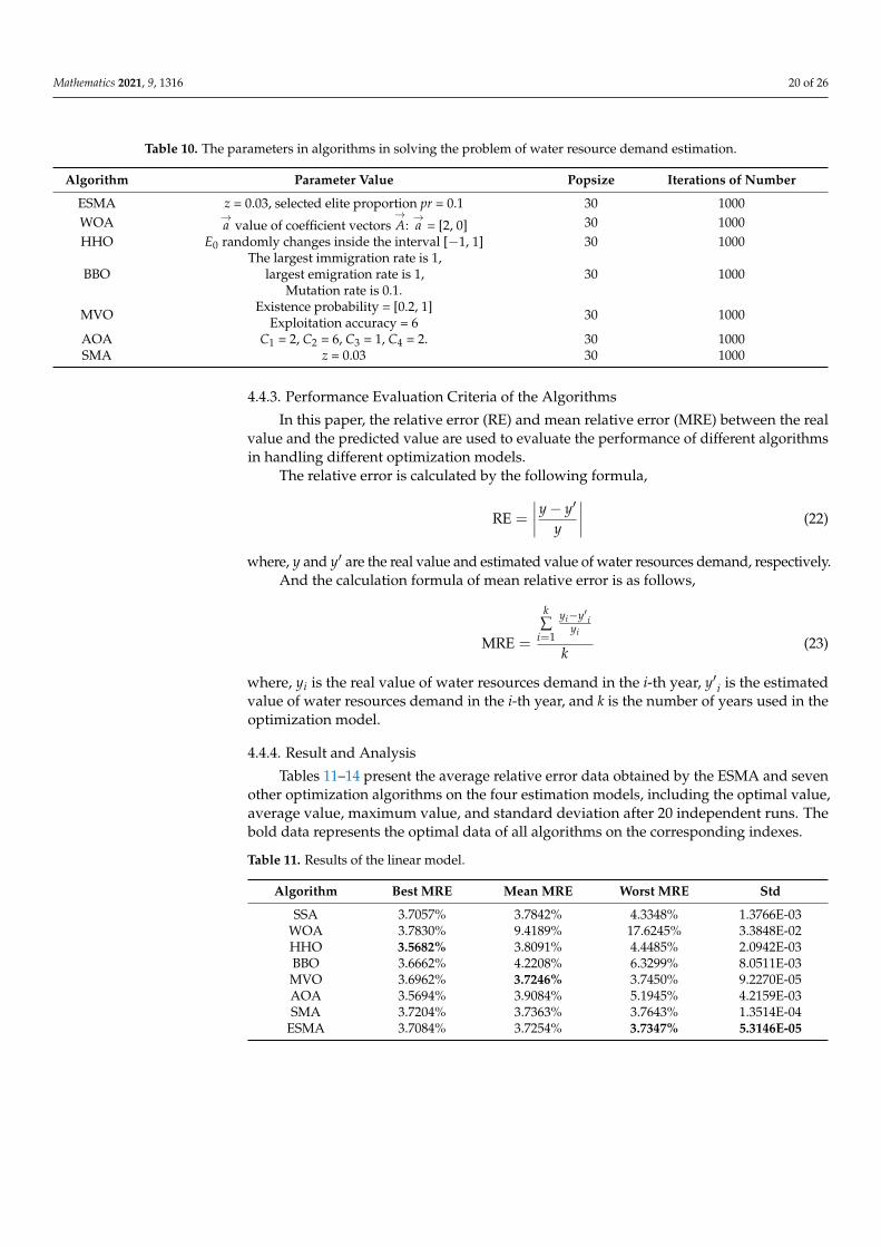
Table 10. The parameters in algorithms in solving the problem of water resource demand estimation.
Algorithm Parameter Value Popsize Iterations of Number
ESMA z = 0.03, selected elite proportion pr = 0.1 30 1000WOA →
a value of coefficient vectors→A:→a = [2, 0] 30 1000
HHO E0 randomly changes inside the interval [−1, 1] 30 1000
BBOThe largest immigration rate is 1,
largest emigration rate is 1,Mutation rate is 0.1.
30 1000
MVO Existence probability = [0.2, 1]Exploitation accuracy = 6 30 1000
AOA C1 = 2, C2 = 6, C3 = 1, C4 = 2. 30 1000SMA z = 0.03 30 1000
4.4.3. Performance Evaluation Criteria of the Algorithms
In this paper, the relative error (RE) and mean relative error (MRE) between the realvalue and the predicted value are used to evaluate the performance of different algorithmsin handling different optimization models.
The relative error is calculated by the following formula,
RE =
∣∣∣∣y− y′
y
∣∣∣∣ (22)
where, y and y′ are the real value and estimated value of water resources demand, respectively.And the calculation formula of mean relative error is as follows,
MRE =
k∑
i=1
yi−y′ iyi
k(23)
where, yi is the real value of water resources demand in the i-th year, y′ i is the estimatedvalue of water resources demand in the i-th year, and k is the number of years used in theoptimization model.
4.4.4. Result and Analysis
Tables 11–14 present the average relative error data obtained by the ESMA and sevenother optimization algorithms on the four estimation models, including the optimal value,average value, maximum value, and standard deviation after 20 independent runs. Thebold data represents the optimal data of all algorithms on the corresponding indexes.
Table 11. Results of the linear model.
Algorithm Best MRE Mean MRE Worst MRE Std
SSA 3.7057% 3.7842% 4.3348% 1.3766E-03WOA 3.7830% 9.4189% 17.6245% 3.3848E-02HHO 3.5682% 3.8091% 4.4485% 2.0942E-03BBO 3.6662% 4.2208% 6.3299% 8.0511E-03MVO 3.6962% 3.7246% 3.7450% 9.2270E-05AOA 3.5694% 3.9084% 5.1945% 4.2159E-03SMA 3.7204% 3.7363% 3.7643% 1.3514E-04
ESMA 3.7084% 3.7254% 3.7347% 5.3146E-05
Mathematics 2021, 9, 1316 21 of 26
Table 12. Results of the logarithmic model.
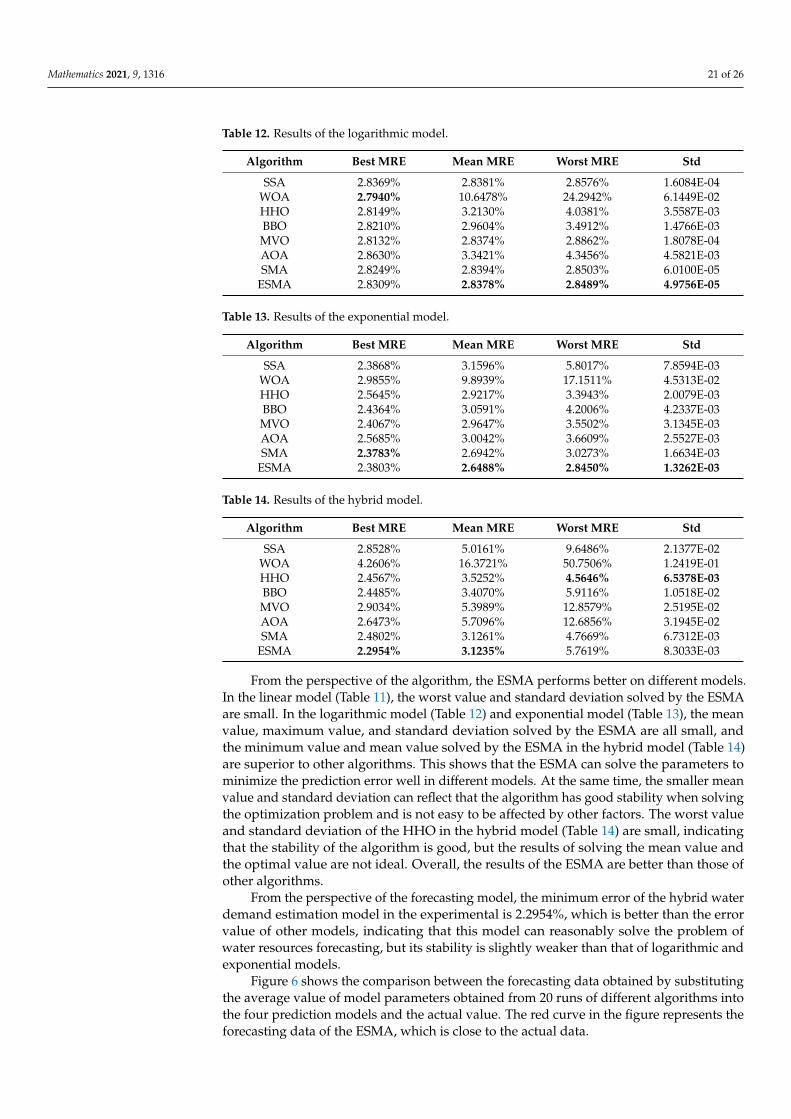
Algorithm Best MRE Mean MRE Worst MRE Std
SSA 2.8369% 2.8381% 2.8576% 1.6084E-04WOA 2.7940% 10.6478% 24.2942% 6.1449E-02HHO 2.8149% 3.2130% 4.0381% 3.5587E-03BBO 2.8210% 2.9604% 3.4912% 1.4766E-03MVO 2.8132% 2.8374% 2.8862% 1.8078E-04AOA 2.8630% 3.3421% 4.3456% 4.5821E-03SMA 2.8249% 2.8394% 2.8503% 6.0100E-05
ESMA 2.8309% 2.8378% 2.8489% 4.9756E-05
Table 13. Results of the exponential model.
Algorithm Best MRE Mean MRE Worst MRE Std
SSA 2.3868% 3.1596% 5.8017% 7.8594E-03WOA 2.9855% 9.8939% 17.1511% 4.5313E-02HHO 2.5645% 2.9217% 3.3943% 2.0079E-03BBO 2.4364% 3.0591% 4.2006% 4.2337E-03MVO 2.4067% 2.9647% 3.5502% 3.1345E-03AOA 2.5685% 3.0042% 3.6609% 2.5527E-03SMA 2.3783% 2.6942% 3.0273% 1.6634E-03
ESMA 2.3803% 2.6488% 2.8450% 1.3262E-03
Table 14. Results of the hybrid model.
Algorithm Best MRE Mean MRE Worst MRE Std
SSA 2.8528% 5.0161% 9.6486% 2.1377E-02WOA 4.2606% 16.3721% 50.7506% 1.2419E-01HHO 2.4567% 3.5252% 4.5646% 6.5378E-03BBO 2.4485% 3.4070% 5.9116% 1.0518E-02MVO 2.9034% 5.3989% 12.8579% 2.5195E-02AOA 2.6473% 5.7096% 12.6856% 3.1945E-02SMA 2.4802% 3.1261% 4.7669% 6.7312E-03
ESMA 2.2954% 3.1235% 5.7619% 8.3033E-03
From the perspective of the algorithm, the ESMA performs better on different models.In the linear model (Table 11), the worst value and standard deviation solved by the ESMAare small. In the logarithmic model (Table 12) and exponential model (Table 13), the meanvalue, maximum value, and standard deviation solved by the ESMA are all small, andthe minimum value and mean value solved by the ESMA in the hybrid model (Table 14)are superior to other algorithms. This shows that the ESMA can solve the parameters tominimize the prediction error well in different models. At the same time, the smaller meanvalue and standard deviation can reflect that the algorithm has good stability when solvingthe optimization problem and is not easy to be affected by other factors. The worst valueand standard deviation of the HHO in the hybrid model (Table 14) are small, indicatingthat the stability of the algorithm is good, but the results of solving the mean value andthe optimal value are not ideal. Overall, the results of the ESMA are better than those ofother algorithms.
From the perspective of the forecasting model, the minimum error of the hybrid waterdemand estimation model in the experimental is 2.2954%, which is better than the errorvalue of other models, indicating that this model can reasonably solve the problem ofwater resources forecasting, but its stability is slightly weaker than that of logarithmic andexponential models.
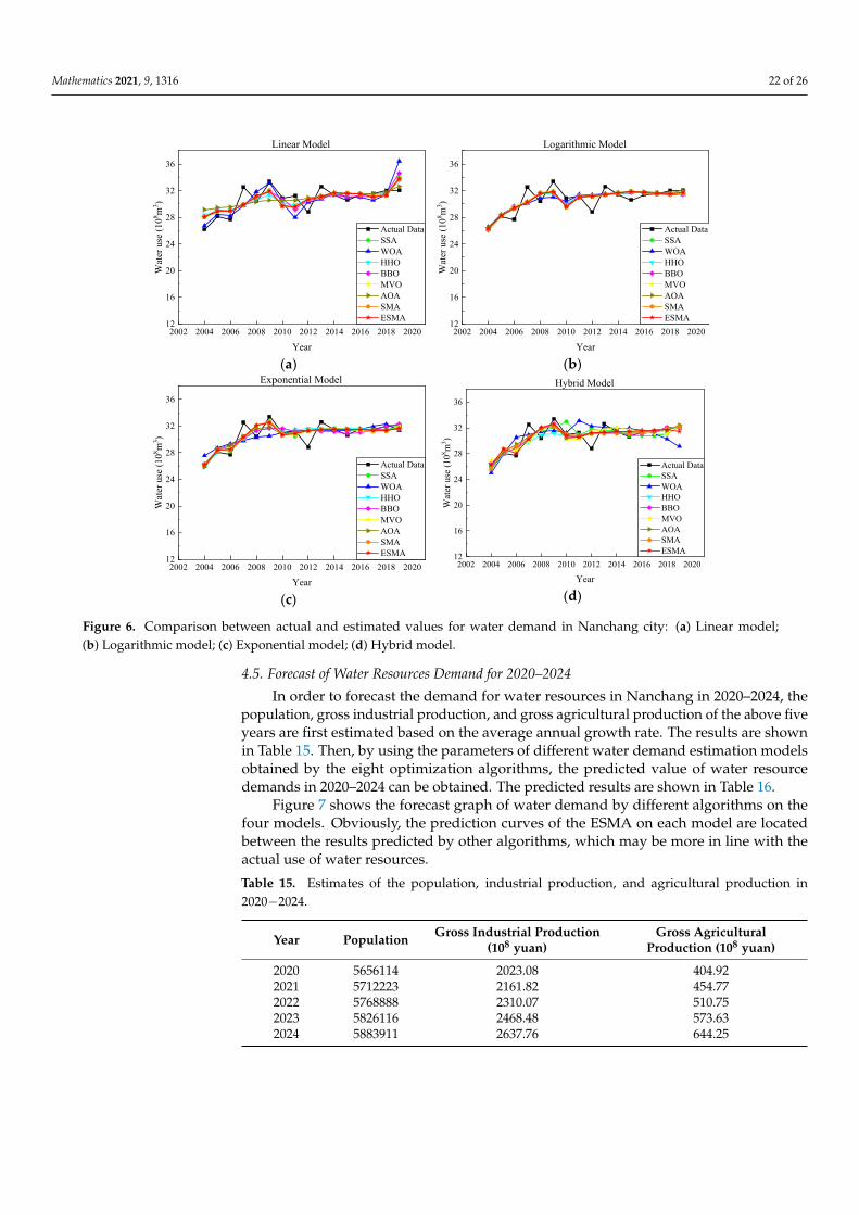
Figure 6 shows the comparison between the forecasting data obtained by substitutingthe average value of model parameters obtained from 20 runs of different algorithms intothe four prediction models and the actual value. The red curve in the figure represents theforecasting data of the ESMA, which is close to the actual data.
Mathematics 2021, 9, 1316 22 of 26
Mathematics 2021, 9, x FOR PEER REVIEW 23 of 27
Figure 6 shows the comparison between the forecasting data obtained by substituting the average value of model parameters obtained from 20 runs of different algorithms into the four prediction models and the actual value. The red curve in the figure represents the forecasting data of the ESMA, which is close to the actual data.
(a)
(b)
(c)
(d)
Figure 6. Comparison between actual and estimated values for water demand in Nanchang city: (a) Linear model; (b) Logarithmic model; (c) Exponential model; (d) Hybrid model.
4.5. Forecast of Water Resources Demand for 2020–2024 In order to forecast the demand for water resources in Nanchang in 2020–2024, the
population, gross industrial production, and gross agricultural production of the above five years are first estimated based on the average annual growth rate. The results are shown in Table 15. Then, by using the parameters of different water demand estimation models obtained by the eight optimization algorithms, the predicted value of water re-source demands in 2020–2024 can be obtained. The predicted results are shown in Table 16.
Table 15. Estimates of the population, industrial production, and agricultural production in 2020−2024.
Year Population Gross Industrial Production (108 yuan) Gross Agricultural Production (108 yuan) 2020 5656114 2023.08 404.92 2021 5712223 2161.82 454.77 2022 5768888 2310.07 510.75 2023 5826116 2468.48 573.63 2024 5883911 2637.76 644.25
2002 2004 2006 2008 2010 2012 2014 2016 2018 202012
16
20
24
28
32
36
Linear ModelW
ater
use
(108 m
3 )
Year
Actual Data SSA WOA HHO BBO MVO AOA SMA ESMA
2002 2004 2006 2008 2010 2012 2014 2016 2018 202012
16
20
24
28
32
36
Wat
er u
se (1
08 m3 )
Year
Actual Data SSA WOA HHO BBO MVO AOA SMA ESMA
Logarithmic Model
2002 2004 2006 2008 2010 2012 2014 2016 2018 202012
16
20
24
28
32
36
Exponential Model
Wat
er u
se (1
08 m3 )
Year
Actual Data SSA WOA HHO BBO MVO AOA SMA ESMA
2002 2004 2006 2008 2010 2012 2014 2016 2018 202012
16
20
24
28
32
36
Hybrid Model
Wat
er u
se (1
08 m3 )
Year
Actual Data SSA WOA HHO BBO MVO AOA SMA ESMA
Figure 6. Comparison between actual and estimated values for water demand in Nanchang city: (a) Linear model;(b) Logarithmic model; (c) Exponential model; (d) Hybrid model.
4.5. Forecast of Water Resources Demand for 2020–2024
In order to forecast the demand for water resources in Nanchang in 2020–2024, thepopulation, gross industrial production, and gross agricultural production of the above fiveyears are first estimated based on the average annual growth rate. The results are shownin Table 15. Then, by using the parameters of different water demand estimation modelsobtained by the eight optimization algorithms, the predicted value of water resourcedemands in 2020–2024 can be obtained. The predicted results are shown in Table 16.
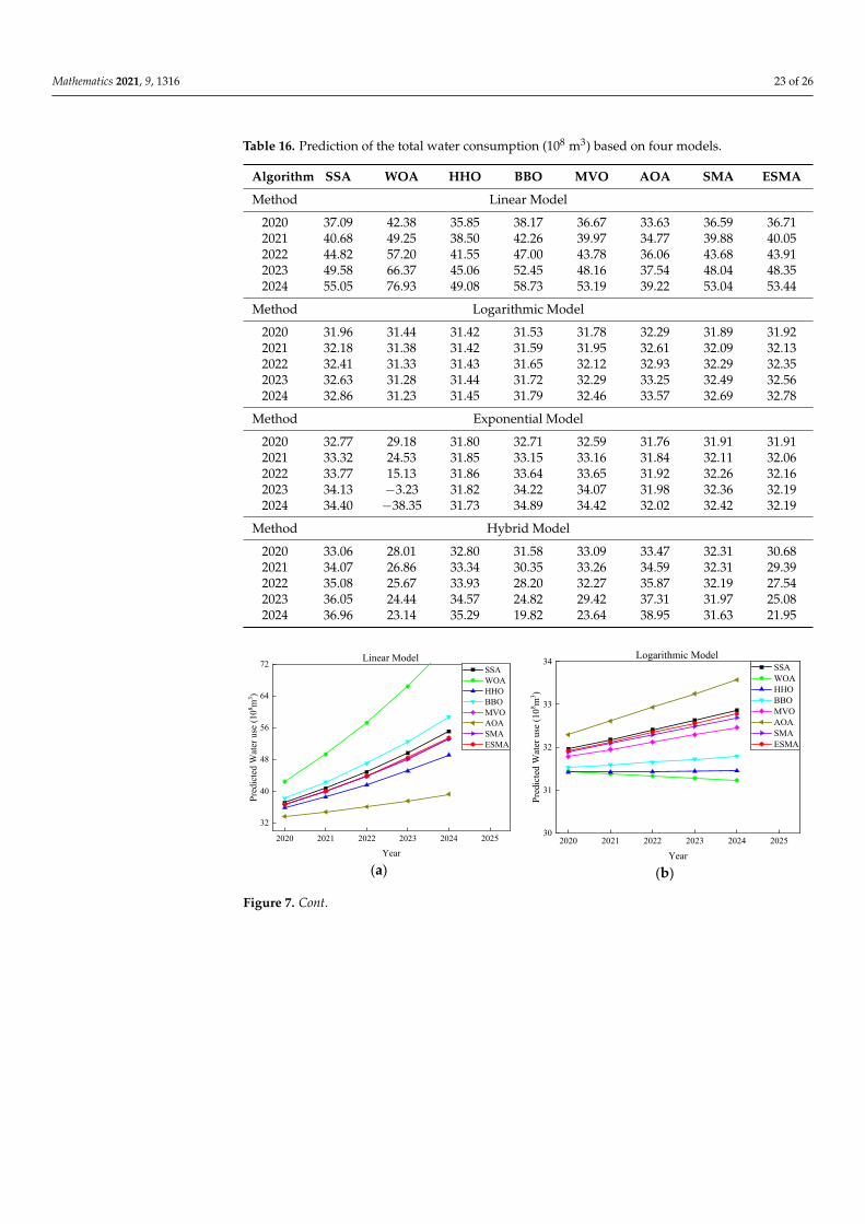
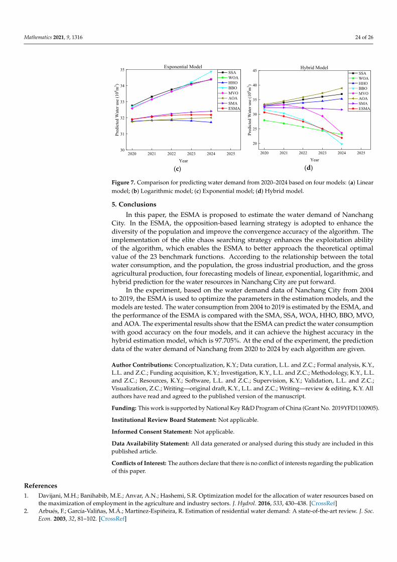
Figure 7 shows the forecast graph of water demand by different algorithms on thefour models. Obviously, the prediction curves of the ESMA on each model are locatedbetween the results predicted by other algorithms, which may be more in line with theactual use of water resources.
Table 15. Estimates of the population, industrial production, and agricultural production in2020−2024.
Year Population Gross Industrial Production(108 yuan)
Gross AgriculturalProduction (108 yuan)
2020 5656114 2023.08 404.922021 5712223 2161.82 454.772022 5768888 2310.07 510.752023 5826116 2468.48 573.632024 5883911 2637.76 644.25
Mathematics 2021, 9, 1316 23 of 26
Table 16. Prediction of the total water consumption (108 m3) based on four models.
Algorithm SSA WOA HHO BBO MVO AOA SMA ESMA
Method Linear Model
2020 37.09 42.38 35.85 38.17 36.67 33.63 36.59 36.712021 40.68 49.25 38.50 42.26 39.97 34.77 39.88 40.052022 44.82 57.20 41.55 47.00 43.78 36.06 43.68 43.912023 49.58 66.37 45.06 52.45 48.16 37.54 48.04 48.352024 55.05 76.93 49.08 58.73 53.19 39.22 53.04 53.44
Method Logarithmic Model
2020 31.96 31.44 31.42 31.53 31.78 32.29 31.89 31.922021 32.18 31.38 31.42 31.59 31.95 32.61 32.09 32.132022 32.41 31.33 31.43 31.65 32.12 32.93 32.29 32.352023 32.63 31.28 31.44 31.72 32.29 33.25 32.49 32.562024 32.86 31.23 31.45 31.79 32.46 33.57 32.69 32.78
Method Exponential Model
2020 32.77 29.18 31.80 32.71 32.59 31.76 31.91 31.912021 33.32 24.53 31.85 33.15 33.16 31.84 32.11 32.062022 33.77 15.13 31.86 33.64 33.65 31.92 32.26 32.162023 34.13 −3.23 31.82 34.22 34.07 31.98 32.36 32.192024 34.40 −38.35 31.73 34.89 34.42 32.02 32.42 32.19
Method Hybrid Model
2020 33.06 28.01 32.80 31.58 33.09 33.47 32.31 30.682021 34.07 26.86 33.34 30.35 33.26 34.59 32.31 29.392022 35.08 25.67 33.93 28.20 32.27 35.87 32.19 27.542023 36.05 24.44 34.57 24.82 29.42 37.31 31.97 25.082024 36.96 23.14 35.29 19.82 23.64 38.95 31.63 21.95
Mathematics 2021, 9, x FOR PEER REVIEW 24 of 27
Table 16. Prediction of the total water consumption (108 m3) based on four models.
Algorithm SSA WOA HHO BBO MVO AOA SMA ESMA Method Linear Model
2020 37.09 42.38 35.85 38.17 36.67 33.63 36.59 36.71 2021 40.68 49.25 38.50 42.26 39.97 34.77 39.88 40.05 2022 44.82 57.20 41.55 47.00 43.78 36.06 43.68 43.91 2023 49.58 66.37 45.06 52.45 48.16 37.54 48.04 48.35 2024 55.05 76.93 49.08 58.73 53.19 39.22 53.04 53.44
Method Logarithmic Model 2020 31.96 31.44 31.42 31.53 31.78 32.29 31.89 31.92 2021 32.18 31.38 31.42 31.59 31.95 32.61 32.09 32.13 2022 32.41 31.33 31.43 31.65 32.12 32.93 32.29 32.35 2023 32.63 31.28 31.44 31.72 32.29 33.25 32.49 32.56 2024 32.86 31.23 31.45 31.79 32.46 33.57 32.69 32.78
Method Exponential Model 2020 32.77 29.18 31.80 32.71 32.59 31.76 31.91 31.91 2021 33.32 24.53 31.85 33.15 33.16 31.84 32.11 32.06 2022 33.77 15.13 31.86 33.64 33.65 31.92 32.26 32.16 2023 34.13 −3.23 31.82 34.22 34.07 31.98 32.36 32.19 2024 34.40 −38.35 31.73 34.89 34.42 32.02 32.42 32.19
Method Hybrid Model 2020 33.06 28.01 32.80 31.58 33.09 33.47 32.31 30.68 2021 34.07 26.86 33.34 30.35 33.26 34.59 32.31 29.39 2022 35.08 25.67 33.93 28.20 32.27 35.87 32.19 27.54 2023 36.05 24.44 34.57 24.82 29.42 37.31 31.97 25.08 2024 36.96 23.14 35.29 19.82 23.64 38.95 31.63 21.95
Figure 7 shows the forecast graph of water demand by different algorithms on the four models. Obviously, the prediction curves of the ESMA on each model are located between the results predicted by other algorithms, which may be more in line with the actual use of water resources.
(a)
(b)
2020 2021 2022 2023 2024 2025
32
40
48
56
64
72 Linear Model
Pred
icte
d W
ater
use
(108 m
3 )
Year
SSA WOA HHO BBO MVO AOA SMA ESMA
2020 2021 2022 2023 2024 202530
31
32
33
34 Logarithmic Model
Pred
icte
d W
ater
use
(108 m
3 )
Year
SSA WOA HHO BBO MVO AOA SMA ESMA
Figure 7. Cont.
Mathematics 2021, 9, 1316 24 of 26Mathematics 2021, 9, x FOR PEER REVIEW 25 of 27
(c)
(d)
Figure 7. Comparison for predicting water demand from 2020–2024 based on four models: (a) Lin-ear model; (b) Logarithmic model; (c) Exponential model; (d) Hybrid model.
5. Conclusions In this paper, the ESMA is proposed to estimate the water demand of Nanchang City.
In the ESMA, the opposition-based learning strategy is adopted to enhance the diversity of the population and improve the convergence accuracy of the algorithm. The implemen-tation of the elite chaos searching strategy enhances the exploitation ability of the algo-rithm, which enables the ESMA to better approach the theoretical optimal value of the 23 benchmark functions. According to the relationship between the total water consumption, and the population, the gross industrial production, and the gross agricultural produc-tion, four forecasting models of linear, exponential, logarithmic, and hybrid prediction for the water resources in Nanchang City are put forward.
In the experiment, based on the water demand data of Nanchang City from 2004 to 2019, the ESMA is used to optimize the parameters in the estimation models, and the mod-els are tested. The water consumption from 2004 to 2019 is estimated by the ESMA, and the performance of the ESMA is compared with the SMA, SSA, WOA, HHO, BBO, MVO, and AOA. The experimental results show that the ESMA can predict the water consump-tion with good accuracy on the four models, and it can achieve the highest accuracy in the hybrid estimation model, which is 97.705%. At the end of the experiment, the prediction data of the water demand of Nanchang from 2020 to 2024 by each algorithm are given.
Author Contributions: Conceptualization, K.Y.; Data curation, L.L. and Z.C.; Formal analysis, K.Y., L.L. and Z.C.; Funding acquisition, K.Y.; Investigation, K.Y., L.L. and Z.C.; Methodology, K.Y., L.L. and Z.C.; Resources, K.Y.; Software, L.L. and Z.C.; Supervision, K.Y.; Validation, L.L. and Z.C.; Vis-ualization, Z.C.; Writing—original draft, K.Y., L.L. and Z.C.; Writing—review & editing, K.Y. All authors have read and agreed to the published version of the manuscript.
Funding: This work is supported by National Key R&D Program of China (Grant No. 2019YFD1100905).
Institutional Review Board Statement: Not applicable.
Informed Consent Statement: Not applicable.
Data Availability Statement: All data generated or analysed during this study are included in this published article (and its supplementary information files).
Conflicts of Interest: The authors declare that there is no conflict of interests regarding the publica-tion of this paper.
References 1. Davijani, M.H.; Banihabib, M.E.; Anvar, A.N.; Hashemi, S.R. Optimization model for the allocation of water resources based on
the maximization of employment in the agriculture and industry sectors. J. Hydrol. 2016, 533, 430–438.
2020 2021 2022 2023 2024 202530
31
32
33
34
35 Exponential Model
Pred
icte
d W
ater
use
(108 m
3 )
Year
SSA WOA HHO BBO MVO AOA SMA ESMA
2020 2021 2022 2023 2024 2025
20
25
30
35
40
45 Hybrid Model
Pred
icte
d W
ater
use
(108 m
3 )
Year
SSA WOA HHO BBO MVO AOA SMA ESMA
Figure 7. Comparison for predicting water demand from 2020–2024 based on four models: (a) Linearmodel; (b) Logarithmic model; (c) Exponential model; (d) Hybrid model.
5. Conclusions
In this paper, the ESMA is proposed to estimate the water demand of NanchangCity. In the ESMA, the opposition-based learning strategy is adopted to enhance thediversity of the population and improve the convergence accuracy of the algorithm. Theimplementation of the elite chaos searching strategy enhances the exploitation abilityof the algorithm, which enables the ESMA to better approach the theoretical optimalvalue of the 23 benchmark functions. According to the relationship between the totalwater consumption, and the population, the gross industrial production, and the grossagricultural production, four forecasting models of linear, exponential, logarithmic, andhybrid prediction for the water resources in Nanchang City are put forward.
In the experiment, based on the water demand data of Nanchang City from 2004to 2019, the ESMA is used to optimize the parameters in the estimation models, and themodels are tested. The water consumption from 2004 to 2019 is estimated by the ESMA, andthe performance of the ESMA is compared with the SMA, SSA, WOA, HHO, BBO, MVO,and AOA. The experimental results show that the ESMA can predict the water consumptionwith good accuracy on the four models, and it can achieve the highest accuracy in thehybrid estimation model, which is 97.705%. At the end of the experiment, the predictiondata of the water demand of Nanchang from 2020 to 2024 by each algorithm are given.
Author Contributions: Conceptualization, K.Y.; Data curation, L.L. and Z.C.; Formal analysis, K.Y.,L.L. and Z.C.; Funding acquisition, K.Y.; Investigation, K.Y., L.L. and Z.C.; Methodology, K.Y., L.L.and Z.C.; Resources, K.Y.; Software, L.L. and Z.C.; Supervision, K.Y.; Validation, L.L. and Z.C.;Visualization, Z.C.; Writing—original draft, K.Y., L.L. and Z.C.; Writing—review & editing, K.Y. Allauthors have read and agreed to the published version of the manuscript.
Funding: This work is supported by National Key R&D Program of China (Grant No. 2019YFD1100905).
Institutional Review Board Statement: Not applicable.
Informed Consent Statement: Not applicable.
Data Availability Statement: All data generated or analysed during this study are included in thispublished article.
Conflicts of Interest: The authors declare that there is no conflict of interests regarding the publicationof this paper.
References1. Davijani, M.H.; Banihabib, M.E.; Anvar, A.N.; Hashemi, S.R. Optimization model for the allocation of water resources based on
the maximization of employment in the agriculture and industry sectors. J. Hydrol. 2016, 533, 430–438. [CrossRef]2. Arbués, F.; García-Valiñas, M.Á.; Martínez-Espiñeira, R. Estimation of residential water demand: A state-of-the-art review. J. Soc.
Econ. 2003, 32, 81–102. [CrossRef]
Mathematics 2021, 9, 1316 25 of 26
3. Hang, L.; Chi, Z.; Dong, M.; Ming, Z. Water demand prediction of Grey Markov model based on GM(1,1). In Proceedings of the2016 3rd International Conference on Mechatronics and Information Technology, Shenzhen, China, 9–10 April 2016.
4. Brentan, B.M.; Luvizotto, E., Jr.; Herrera, M.; Lzquierdo, J.; Pérez-García, R. Hybrid regression model for near real-time urbanwater demand forecasting. J. Comput. Appl. Math. 2017, 309, 532–541. [CrossRef]
5. Al-Zahrani, M.A.; Abo-Monasar, A. Urban Residential Water Demand Prediction Based on Artificial Neural Networks and TimeSeries Models. Water Resour. Manag. 2015, 29, 3651–3662. [CrossRef]
6. Bai, Y.; Wang, P.; Li, C.; Xie, J.J.; Wang, Y. A multi-scale relevance vector regression approach for daily urban water demandforecasting. J. Hydrol. 2014, 517, 236–245. [CrossRef]
7. Pulido-Calvo, I.; Gutiérrez-Estrada, J.C. Improved irrigation water demand forecasting using a soft-computing hybrid model.Biosyst. Eng. 2009, 102, 202–218. [CrossRef]
8. Romano, M.; Kapelan, Z. Adaptive water demand forecasting for near real-time management of smart water distribution systems.Environ. Modell. Softw. 2014, 60, 265–276. [CrossRef]
9. Oliveira, P.J.; Steffen, J.L.; Cheung, P. Parameter estimation of seasonal arima models for water demand forecasting using theharmony search algorithm. Procedia Eng. 2017, 186, 177–185. [CrossRef]
10. Kennedy, J.; Eberhart, R.C. Particle swarm optimization. In Proceedings of the IEEE International Conference on Neural Networks,Perth, WA, Australia, 27 November–1 December 1995; pp. 1942–1948.
11. Mirjalili, S.; Lewis, A. The whale optimization algorithm. Adv. Eng. Soft. 2016, 95, 51–67. [CrossRef]12. Mirjalili, S.; Mirjalili, S.M.; Lewis, A. Grey wolf optimizer. Adv. Eng. Soft. 2014, 69, 46–61. [CrossRef]13. Heidari, A.; Mirjalili, S.; Farris, H.; Aljarah, I.; Mafarja, M.; Chen, H. Harris hawks optimization: Algorithm and applications.
Future Gener. Comput. Syst. 2019, 97, 849–872. [CrossRef]14. Yang, X.S. Firefly algorithm, stochastic test functions and design optimization. Int. J. Bio Inspir. Comput. 2010, 2, 78–84. [CrossRef]15. Zhao, W.G.; Zhang, Z.X.; Wang, L.Y. Manta ray foraging optimization: An effective bio-inspired optimizer for engineering
applications. Eng. Appl. Artif. Intell. 2020, 87, 103300. [CrossRef]16. Faramarzi, A.; Heidarinejad, M.; Mirjalil, S.; Gandomi, A.H. Marine Predators Algorithm: A nature-inspired metaheuristic. Expert
Syst. Appl. 2020, 152, 113377. [CrossRef]17. Li, S.M.; Chen, H.L.; Wang, M.J.; Heidari, A.A.; Mirjalili, S. Slime mould algorithm: A new method for stochastic optimization.
Future Gener. Comput. Syst. 2020, 111, 300–323. [CrossRef]18. Vashishtha, G.; Chauhan, S.; Singh, M.; Kumar, R. Bearing defect identification by swarm decomposition considering permutation
entropy measure and opposition-based slime mould algorithm. Measurement 2021, 178, 109389. [CrossRef]19. Mostafa, M.; Rezk, H.; Aly, M.; Ahmed, E.M. A new strategy based on slime mould algorithm to extract the optimal model
parameters of solar PV panel. Sustain. Energy Techn. 2020, 42, 100849. [CrossRef]20. Abdel-Basset, M.; Mohamed, R.; Chakrabortty, R.K.; Ryan, M.J.; Mirjalili, S. An efficient binary slime mould algorithm integrated
with a novel attacking-feeding strategy for feature selection. Comput. Ind. Eng. 2021, 153, 107078. [CrossRef]21. Kumar, C.; Raj, T.D.; Premkumar, M.; Raj, T.D. A new stochastic slime mould optimization algorithm for the estimation of solar
photovoltaic cell parameters. Optik 2020, 223, 165277. [CrossRef]22. Rizk-Allah, R.M.; Hassanien, A.E.; Song, D.R. Chaos-opposition-enhanced slime mould algorithm for minimizing the cost of
energy for the wind turbines on high-altitude sites. ISA Trans. 2021, in press. [CrossRef]23. Abdel-Basset, M.; Chang, V.; Mohamed, R. HSMA_WOA: A hybrid novel Slime mould algorithm with whale optimization
algorithm for tackling the image segmentation problem of chest X-ray images. Appl. Soft Comput. 2020, 95, 106642. [CrossRef]24. Houssein, E.H.; Mahdy, M.A.; Blondin, M.J.; Shebl, D.; Mohamed, W.M. Hybrid slime mould algorithm with adaptive guided dif-
ferential evolution algorithm for combinatorial and global optimization problems. Expert Syst. Appl. 2021, 174, 114689. [CrossRef]25. Djekidel, R.; Bentouati, B.; Javaid, M.S.; Bouchekara, H.R.E.H.; Bayoumi, A.S.; El-Sehiemy, R.A. Mitigating the effects of magnetic
coupling between HV Transmission Line and Metallic Pipeline using Slime Mould Algorithm. J. Magn. Magn. Mater. 2021,529, 167865. [CrossRef]
26. El-Fergany, A.A. Parameters identification of PV model using improved slime mould optimizer and Lambert W-function. EnergyRep. 2021, 7, 875–887. [CrossRef]
27. Tizhoosh, R.H. Opposition-based learning: A new scheme for machine intelligence. In Proceedings of the International Conferenceon Computational Intelligence for Modelling, Control & Automation and International Conference on Intelligent Agents, Vienna,Austria, 28–30 November 2005; pp. 695–701.
28. Muthusamy, H.; Ravindran, S.; Yaacob, S.; Polat, K. An improved elephant herding optimization using sine-cosine mechanismand opposition based learning for global optimization problems. Expert Syst. Appl. 2021, 172, 114607. [CrossRef]
29. Mirjalili, S. The ant lion optimizer. Adv. Eng. Soft. 2015, 83, 80–98. [CrossRef]30. Mirjalili, S. SCA: A Sine Cosine Algorithm for solving optimization problems. Knowl. Based Syst. 2016, 96, 120–133. [CrossRef]31. Mirjalili, S. Moth-flame optimization algorithm: A novel nature-inspired heuristic paradigm. Knowl. Based Syst. 2015,
89, 228–249. [CrossRef]32. Mirjalili, S.; Gandomi, A.H.; Mirjalili, S.Z.; Saremi, S.; Faris, H.; Mirjalili, S.M. Salp swarm algorithm: A bio-inspired optimizer for
engineering design problems. Adv. Eng. Soft. 2017, 114, 163–191. [CrossRef]33. Xing, B.; Gao, W.J. Biogeography—Based Optimization Algorithm; Springer: Berlin/Heidelberg, Germany, 2014.

Mathematics 2021, 9, 1316 26 of 26
34. Mirjalili, S.; Mirjalili, S.M.; Hatamlou, A. Multi-Verse Optimizer: A nature-inspired algorithm for global optimization. NeuralComput. Appl. 2015, 27, 495–513. [CrossRef]
35. Hashim, F.A.; Hussain, K.; Houssein, E.H.; Mai, S.M.; Ai-Atabany, W. Archimedes optimization algorithm: A new metaheuristicalgorithm for solving optimization problems. Appl. Intell. 2021, 51, 1531–1551. [CrossRef]