An Improved Schur–Pade Algorithm for Fractional Powers of ...eprints.ma.man.ac.uk/2021/01/covered/MIMS_ep2013_1.pdf · An Improved Schur–Pade Algorithm for Fractional Powers of

An Improved Schur–Pade Algorithm forFractional Powers of a Matrix and their Frechet

Derivatives

Higham, Nicholas J. and Lin, Lijing

2013

MIMS EPrint: 2013.1

Manchester Institute for Mathematical SciencesSchool of Mathematics

The University of Manchester

Reports available from: http://eprints.maths.manchester.ac.uk/And by contacting: The MIMS Secretary

School of Mathematics

The University of Manchester

Manchester, M13 9PL, UK

ISSN 1749-9097

http://eprints.maths.manchester.ac.uk/

Copyright © by SIAM. Unauthorized reproduction of this article is prohibited.

SIAM J. MATRIX ANAL. APPL. c© 2013 Society for Industrial and Applied MathematicsVol. 34, No. 3, pp. 1341–1360

AN IMPROVED SCHUR–PADE ALGORITHM FOR FRACTIONALPOWERS OF A MATRIX AND THEIR FRECHET DERIVATIVES∗

NICHOLAS J. HIGHAM† AND LIJING LIN†

Abstract. The Schur–Pade algorithm [N. J. Higham and L. Lin, SIAM J. Matrix Anal. Appl.,32 (2011), pp. 1056–1078] computes arbitrary real powers At of a matrix A ∈ Cn×n using thebuilding blocks of Schur decomposition, matrix square roots, and Pade approximants. We improvethe algorithm by basing the underlying error analysis on the quantities ‖(I − A)k‖1/k , for severalsmall k, instead of ‖I−A‖. We extend the algorithm so that it computes along with At one or moreFrechet derivatives, with reuse of information when more than one Frechet derivative is required, asis the case in condition number estimation. We also derive a version of the extended algorithm thatworks entirely in real arithmetic when the data is real. Our numerical experiments show the newalgorithms to be superior in accuracy to, and often faster than, the original Schur–Pade algorithmfor computing matrix powers and more accurate than several alternative methods for computing theFrechet derivative. They also show that reliable estimates of the condition number of At are obtainedby combining the algorithms with a matrix norm estimator.

Key words. matrix power, fractional power, matrix root, Frechet derivative, condition number,condition estimate, Schur decomposition, Pade approximation, Pade approximant, matrix logarithm,matrix exponential, MATLAB

AMS subject classification. 65F30

DOI. 10.1137/130906118

1. Introduction. We recently developed a Schur–Pade algorithm [25] for com-puting arbitrary real powers At of a matrix A ∈ C

n×n. The algorithm combines aSchur decomposition with the evaluation of a Pade approximant at a suitably trans-formed Schur factor. That work was motivated by the increasing appearance of frac-tional matrix powers in a variety of applications. In addition to the literature citedin [25], we mention relevant recent work on fractional differential equations by Ben-son, Meerschaert, and Revielle [8], Burrage, Hale, and Kay [12], and Ilic, Turner, andAnh [31].

We recall that for A ∈ Cn×n having no eigenvalues on the closed negative real axisR

−, the principal matrix power At is defined as exp(t logA), where log is the principallogarithm (the one whose eigenvalues have imaginary parts in the interval (−π, π) [24,Thm. 1.31]). Without loss of generality we assume throughout that t ∈ (−1, 1). Forgeneral t ∈ R we can write t = m + f , where m ∈ Z and f ∈ (−1, 1), and thenAt = AmAf . How to choose between the two possible pairs (m, f) is explained in [25,sect. 6].

This work has three aims: to improve the accuracy and efficiency of the Schur–Pade algorithm by sharpening the underlying error analysis, to extend the algorithmso that it computes the Frechet derivative, and to develop a version of the extendedalgorithm that works entirely in real arithmetic when the data is real. The need for

∗Received by the editors January 18, 2013; accepted for publication (in revised form) by M.Van Barel May 29, 2013; published electronically September 17, 2013. This work was supported byEuropean Research Council Advanced grant MATFUN (267526).

http://www.siam.org/journals/simax/34-3/90611.html†School of Mathematics, The University of Manchester, Manchester, M13 9PL, UK

([email protected], http://www.maths.manchester.ac.uk/˜higham, [email protected], http://www.maths.manchester.ac.uk/˜lijing).

1341

Dow

nloa

ded

09/1

7/13

to 1

30.8

8.12

3.32

. Red

istr

ibut

ion

subj

ect t

o SI

AM

lice

nse

or c

opyr

ight

; see

http

://w

ww

.sia

m.o

rg/jo

urna

ls/o

jsa.

php


1342 NICHOLAS J. HIGHAM AND LIJING LIN

a more sophisticated error analysis is illustrated by the upper triangular matrix

(1.1) A =

⎡⎣ 1 1016 00 1 1016

0 0 1

⎤⎦ .

For any t ∈ (−1, 1) the Schur–Pade algorithm of [25] takes 108 square roots of Athen evaluates rm(I − A) for some m ≤ 7, where rm(x) denotes the [m/m] Padeapproximant to (1− x)t. However, no square roots are necessary: since (I −A)k = 0for k ≥ 3, the error in rm(I −A) is zero for any m ≥ 1. By estimating the quantities‖(I − A)k‖1/k for a few k, our new Algorithm 3.1 requires no square roots for thismatrix, and returns a result with the same (high) accuracy as that from the originalalgorithm.

The Frechet derivative of a general matrix function f on Cn×n is a linear operator

Lf (·, E) satisfying

f(A+ E) = f(A) + Lf (A,E) + o(‖E‖)for all E ∈ Cn×n. The Frechet derivative therefore describes the sensitivity of f tosmall perturbations, and can be used to define a condition number

(1.2) cond(f,A) := limε→0

sup‖E‖≤ε‖A‖

‖f(A+ E)− f(A)‖ε‖f(A)‖ =

‖Lf(A)‖‖A‖‖f(A)‖ ,

where

(1.3) ‖Lf(A)‖ := maxZ �=0

‖Lf(X,Z)‖‖Z‖

[24, sect. 3.1]. We develop an algorithm for computing Lxt by Frechet differentiatingour algorithm for At. We then use the algorithm in conjunction with a matrix normestimator to estimate cond(xt, A). By replacing the Schur decomposition with a realSchur decomposition in the case where A and E are real, we derive an algorithm thatworks entirely in real arithmetic, thereby halving the required intermediate storageand halving the number of (real) arithmetic operations required.

In section 2 we extend the analysis of [25] for the error in Pade approximants of(1 − x)t evaluated at a matrix argument X ∈ Cn×n to use the quantities ‖Xk‖1/kinstead of ‖X‖. In section 3 we develop a Schur–Pade algorithm based on thesebounds. In section 4 we extend the algorithm to compute both At and the Frechetderivative Lxt(A,E) and make comparisons with other approaches to computing theFrechet derivative. In section 5 we modify the algorithms so that they use only realarithmetic when A and E are real. In section 6 we explain how to use the algorithms toestimate the condition number of At, based on evaluations of Lxt(A,E) for several E.Numerical experiments that compare the new algorithms with existing ones are givenin section 7 and conclusions are given in section 8.

2. Forward error analysis. The Schur–Pade algorithm of Higham and Lin [25]computes a Schur decomposition A = QTQ∗ (Q unitary, T upper triangular), takess square roots of T , evaluates the [m/m] Pade approximant rm(x) of (1 − x)t atI − T 1/2s , squares the result s times, then transforms back. The choice of m ands in the algorithm is based on the forward error bound in the following theorem.The norm here is any subordinate matrix norm and rkm(x) denotes the [k/m] Padeapproximant to (1 − x)t.

Dow

nloa

ded

09/1

7/13

to 1

30.8

8.12

3.32

. Red

istr

ibut

ion

subj

ect t

o SI

AM

lice

nse

or c

opyr

ight

; see

http

://w

ww

.sia

m.o

rg/jo

urna

ls/o

jsa.

php


FRACTIONAL MATRIX POWERS AND FRECHET DERIVATIVES 1343

Theorem 2.1 (see [25, Thm. 3.5]). Let X ∈ Cn×n with ‖X‖ < 1. For k ≥ mand −1 < t < 1,

(2.1) ‖(I −X)t − rkm(X)‖ ≤ |(1 − ‖X‖)t − rkm(‖X‖)|.

In particular, when −1 < t < 0, (2.1) holds for k ≥ m− 1.The bound in Theorem 2.1 can be sharpened by applying the technique of Al-

Mohy and Higham [3] in order to base the error bound on the quantities

αp(X) = max(‖Xp‖1/p, ‖Xp+1‖1/(p+1)

),(2.2)

where the integer p ≥ 1. As explained in [3], ρ(X) ≤ αp(X) ≤ ‖X‖, where ρ isthe spectral radius, and αp(X) � ‖X‖ is possible for nonnormal X . Moreover,if h�(x) =

∑∞i=� cix

i is a power series with radius of convergence ω then, from [3,Thm. 4.2(a)], for any X ∈ Cn×n with ρ(X) < ω we have ‖h�(X)‖ ≤∑∞

i=� |ci|αp(X)i

for p satisfying p(p − 1) ≤ �. A new error bound in terms of the αi is given in thenext result.

Theorem 2.2. Let X ∈ Cn×n with ρ(X) < 1. For k ≥ m and −1 < t < 1, andfor k ≥ m− 1 and −1 < t < 0,

(2.3) (I −X)t − rkm(X) =

∞∑i=k+m+1

ψiXi,

where every coefficient ψi ≡ ψi(t, k,m) has the same sign. Moreover,

(2.4) ‖(I −X)t − rkm(X)‖ ≤ |(1 − αp(X))t − rkm(αp(X))|,

where αp is defined in (2.2) and p satisfies

(2.5) k +m+ 1 ≥ p(p− 1).

Proof. The error in the [k/m] Pade approximant rkm(x) to (1−x)t can be written[25, Lem. 3.4]

(1− x)t − rkm(x) = qkm(1)qkm(x)−1∞∑

i=k+m+1

(−t)i(i− (k +m))mi!(i− t−m)m

xi, |x| < 1,

where qkm is the denominator of rkm with qkm(0) = 1 and (a)i ≡ a(a+1) . . . (a+i−1)with (a)0 = 1. We can write qkm(x) = c

∏mi=1(xi − x), where xi, i = 1: m, are the

zeros of qkm(x) and c =∏m

i=1 x−1i . Assuming k ≥ m, from [25, Cor. 3.3], [33, Cor. 1]

we have xi > 1 for all i. Hence if |x| < 1,

qkm(x)−1 =

m∏i=1

(1− x

xi

)−1

=

m∏i=1

(1 +

x

xi+x2

x2i+ · · ·

)=:

∞∑i=0

dixi,

where di > 0. (That di > 0 also follows when t ∈ (−1, 0) from a more general resultof Gomilko, Greco, and Zietak [19, Cor. 5.6].)

It follows that for any t ∈ (−1, 1), in the error expansion (1 − x)t − rkm(x) =∑∞i=k+m+1 ψix

i each ψi has the same sign. Therefore (2.3) holds for ρ(X) < 1.Finally, by applying [3, Thm. 4.2(a)] to (2.3), we obtain

Dow

nloa

ded

09/1

7/13

to 1

30.8

8.12

3.32

. Red

istr

ibut

ion

subj

ect t

o SI

AM

lice

nse

or c

opyr

ight

; see

http

://w

ww

.sia

m.o

rg/jo

urna

ls/o

jsa.

php



‖(I −X)t − rkm(X)‖ ≤∞∑

i=k+m+1

|ψi|αp(X)i

=

∣∣∣∣∣∞∑

i=k+m+1

ψiαp(X)i

∣∣∣∣∣ =∣∣(1− αp(X))t − rkm(αp(X))

∣∣for p satisfying (2.5).

If −1 < t < 0, it follows from [25, Cor. 3.3], [33, Cor. 1] that the roots xiof qkm satisfy xi > 1 for k ≥ m − 1, so the conclusion of the theorem holds fork ≥ m− 1.

3. Improved Schur–Pade algorithm. Whereas the Schur–Pade algorithm of[25] is based on the norm of I − T 1/2s , through the use of (2.1), here we will exploit(2.4), which uses the generally smaller quantities αp(I − T 1/2s), p ≥ 1. We requirethat αp ≡ αp(I − T 1/2s) satisfies

(3.1) |(1− αp)t − rm(αp)| ≤ u,

where u = 2−53 ≈ 1.1 × 10−16 is the unit roundoff for IEEE double precision arith-metic, which by (2.4) ensures double precision accuracy of the Pade approximant. For

given t and m, we denote by θ(t)m the largest θ such that |(1 − θ)t − rm(θ)| ≤ u, and

define

(3.2) θm = min{ θ(t)m : t ∈ [−1, 1] }.

The values of θm, determined in [25], are shown in Table 3.1. Our algorithm requiresthat αp(I − T 1/2s) ≤ θm for some p satisfying p(p− 1) ≤ 2m+ 1.

As in [25] we compute square roots of triangular matrices by the Bjorck andHammarling recurrence [11], [24, Alg. 6.3], which costs n3/3 flops, and we computerm by evaluating its continued fraction form in bottom-up fashion (see section 4.2),which costs 2mn3/3 flops.

Our overall aim is to choose the parameters s and m to minimize the total costsubject to (3.1). The following reasoning is adapted from that used to derive aninverse scaling and squaring algorithm for the matrix logarithm that is also based onthe αp [4]. Although the θm and the cost of evaluating the Pade approximant aredifferent than in the logarithm case, the algorithm turns out (perhaps surprisingly)to have exactly the same form.

For any putative s and m satisfying αp(I − T 1/2s) ≤ θm for some p, it is worthtaking one more square root (costing n3/3 flops) if it allows a reduction in the Padedegree m by more than one (resulting in a saving of at least 2n3/3 flops once the extra

squarings are taken into account), that is, if αp(I−T 1/2s+1

) ≤ θm−2 for some p. Since

(I−T 1/2s+1

)(I+T 1/2s+1

) = I−T 1/2s , we have that αp(I−T 1/2s+1

) ≈ 12αp(I−T 1/2s),

for suitably large s. Since θm/2 < θm−2 for m > 7, the cost of computing T t willbe minimized if we take square roots of T repeatedly until αp(I − T 1/2s) ≤ θ7 forsome p ∈ {1, 2, 3, 4} (see Table 3.2). Some work can be saved by using the fact thatρ(I − D) = ρ(I − T ) ≤ αp(I − T ), where D = diag(T ), and so there is no need tocompute αp(I−T 1/2s) until ρ(I−D1/2s) ≤ θ7; let us denote the smallest such s by s0.

After obtaining s0 and computing T ← T 1/2s0 , we first check if m = 1 or m = 2can be used, since no more square roots need to be taken in this case. If m = 1 andm = 2 are ruled out we now determine whether more square roots are needed and

Dow

nloa

ded

09/1

7/13

to 1

30.8

8.12

3.32

. Red

istr

ibut

ion

subj

ect t

o SI

AM

lice

nse

or c

opyr

ight

; see

http

://w

ww

.sia

m.o

rg/jo

urna

ls/o

jsa.

php



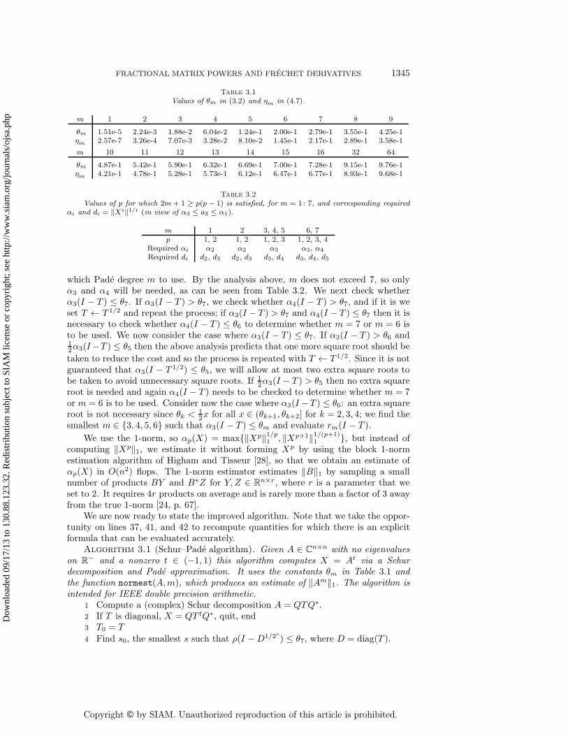
Table 3.1

Values of θm in (3.2) and ηm in (4.7).

m 1 2 3 4 5 6 7 8 9

θm 1.51e-5 2.24e-3 1.88e-2 6.04e-2 1.24e-1 2.00e-1 2.79e-1 3.55e-1 4.25e-1ηm 2.57e-7 3.26e-4 7.07e-3 3.28e-2 8.10e-2 1.45e-1 2.17e-1 2.89e-1 3.58e-1

m 10 11 12 13 14 15 16 32 64

θm 4.87e-1 5.42e-1 5.90e-1 6.32e-1 6.69e-1 7.00e-1 7.28e-1 9.15e-1 9.76e-1ηm 4.21e-1 4.78e-1 5.28e-1 5.73e-1 6.12e-1 6.47e-1 6.77e-1 8.93e-1 9.68e-1

Table 3.2

Values of p for which 2m + 1 ≥ p(p − 1) is satisfied, for m = 1: 7, and corresponding requiredαi and di = ‖Xi‖1/i (in view of α3 ≤ a2 ≤ α1).

m 1 2 3, 4, 5 6, 7p 1, 2 1, 2 1, 2, 3 1, 2, 3, 4

Required αi α2 α2 α3 α3, α4

Required di d2, d3 d2, d3 d3, d4 d3, d4, d5

which Pade degree m to use. By the analysis above, m does not exceed 7, so onlyα3 and α4 will be needed, as can be seen from Table 3.2. We next check whetherα3(I − T ) ≤ θ7. If α3(I − T ) > θ7, we check whether α4(I − T ) > θ7, and if it is weset T ← T 1/2 and repeat the process; if α3(I − T ) > θ7 and α4(I − T ) ≤ θ7 then it isnecessary to check whether α4(I − T ) ≤ θ6 to determine whether m = 7 or m = 6 isto be used. We now consider the case where α3(I − T ) ≤ θ7. If α3(I − T ) > θ6 and12α3(I−T ) ≤ θ5 then the above analysis predicts that one more square root should be

taken to reduce the cost and so the process is repeated with T ← T 1/2. Since it is notguaranteed that α3(I − T 1/2) ≤ θ5, we will allow at most two extra square roots tobe taken to avoid unnecessary square roots. If 1

2α3(I − T ) > θ5 then no extra squareroot is needed and again α4(I − T ) needs to be checked to determine whether m = 7or m = 6 is to be used. Consider now the case where α3(I −T ) ≤ θ6: an extra squareroot is not necessary since θk <

12x for all x ∈ (θk+1, θk+2] for k = 2, 3, 4; we find the

smallest m ∈ {3, 4, 5, 6} such that α3(I − T ) ≤ θm and evaluate rm(I − T ).We use the 1-norm, so αp(X) = max{‖Xp‖1/p1 , ‖Xp+1‖1/(p+1)

1 }, but instead ofcomputing ‖Xp‖1, we estimate it without forming Xp by using the block 1-normestimation algorithm of Higham and Tisseur [28], so that we obtain an estimate ofαp(X) in O(n2) flops. The 1-norm estimator estimates ‖B‖1 by sampling a smallnumber of products BY and B∗Z for Y, Z ∈ Rn×r, where r is a parameter that weset to 2. It requires 4r products on average and is rarely more than a factor of 3 awayfrom the true 1-norm [24, p. 67].

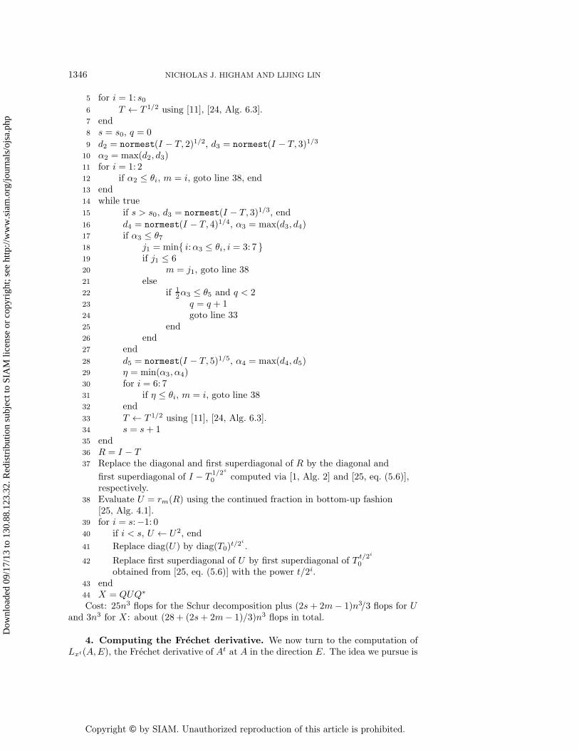
We are now ready to state the improved algorithm. Note that we take the oppor-tunity on lines 37, 41, and 42 to recompute quantities for which there is an explicitformula that can be evaluated accurately.

Algorithm 3.1 (Schur–Pade algorithm). Given A ∈ Cn×n with no eigenvalueson R− and a nonzero t ∈ (−1, 1) this algorithm computes X = At via a Schurdecomposition and Pade approximation. It uses the constants θm in Table 3.1 andthe function normest(A,m), which produces an estimate of ‖Am‖1. The algorithm isintended for IEEE double precision arithmetic.

1 Compute a (complex) Schur decomposition A = QTQ∗.2 If T is diagonal, X = QT tQ∗, quit, end3 T0 = T

4 Find s0, the smallest s such that ρ(I −D1/2s) ≤ θ7, where D = diag(T ).

Dow

nloa

ded

09/1

7/13

to 1

30.8

8.12

3.32

. Red

istr

ibut

ion

subj

ect t

o SI

AM

lice

nse

or c

opyr

ight

; see

http

://w

ww

.sia

m.o

rg/jo

urna

ls/o

jsa.

php



5 for i = 1: s06 T ← T 1/2 using [11], [24, Alg. 6.3].7 end8 s = s0, q = 0

9 d2 = normest(I − T, 2)1/2, d3 = normest(I − T, 3)1/310 α2 = max(d2, d3)11 for i = 1: 212 if α2 ≤ θi, m = i, goto line 38, end13 end14 while true15 if s > s0, d3 = normest(I − T, 3)1/3, end16 d4 = normest(I − T, 4)1/4, α3 = max(d3, d4)17 if α3 ≤ θ718 j1 = min{ i:α3 ≤ θi, i = 3: 7 }19 if j1 ≤ 620 m = j1, goto line 3821 else22 if 1

2α3 ≤ θ5 and q < 223 q = q + 124 goto line 3325 end26 end27 end

28 d5 = normest(I − T, 5)1/5, α4 = max(d4, d5)29 η = min(α3, α4)30 for i = 6: 731 if η ≤ θi, m = i, goto line 3832 end

33 T ← T 1/2 using [11], [24, Alg. 6.3].34 s = s+ 135 end36 R = I − T37 Replace the diagonal and first superdiagonal of R by the diagonal and

first superdiagonal of I − T 1/2s

0 computed via [1, Alg. 2] and [25, eq. (5.6)],respectively.

38 Evaluate U = rm(R) using the continued fraction in bottom-up fashion[25, Alg. 4.1].

39 for i = s:−1: 040 if i < s, U ← U2, end

41 Replace diag(U) by diag(T0)t/2i .

42 Replace first superdiagonal of U by first superdiagonal of Tt/2i

0

obtained from [25, eq. (5.6)] with the power t/2i.43 end44 X = QUQ∗

Cost: 25n3 flops for the Schur decomposition plus (2s+ 2m− 1)n3/3 flops for Uand 3n3 for X : about (28 + (2s+ 2m− 1)/3)n3 flops in total.

4. Computing the Frechet derivative. We now turn to the computation ofLxt(A,E), the Frechet derivative of At at A in the direction E. The idea we pursue is

Dow

nloa

ded

09/1

7/13

to 1

30.8

8.12

3.32

. Red

istr

ibut

ion

subj

ect t

o SI

AM

lice

nse

or c

opyr

ight

; see

http

://w

ww

.sia

m.o

rg/jo

urna

ls/o

jsa.

php



to simultaneously compute At and Lxt(A,E) in a way that reuses matrix operationsfrom the computation of At in the computation of Lxt(A,E).

Recall that At is approximated by (ignoring the Schur decomposition forsimplicity)

At = (A1/2s)t·2s

= (I −X)t·2s ≈ rm(X)2

s

,

where I−X = A1/2s and ρ(X) < 1. Differentiating At = ((A1/2)t)2 and applying thechain rule [24, Thm. 3.4], we obtain

(4.1) Lxt(A,E) = At/2Lxt(A1/2, E1) + Lxt(A1/2, E1)At/2,

where E1 = Lx1/2(A,E) and so A1/2E1 + E1A1/2 = E. Using this relation we can

construct the following recurrences for computing Lxt(A,E). First we form

E0 = E, X0 = A,

Xi = X1/2i−1

Solve XiEi + EiXi = Ei−1 for Ei

}i = 1: s,(4.2)

after which Es = Lx1/2s (A,E) and Xs = A1/2s , and then

Ys = rm(I −Xs), Ls ≈ Lxt(Xs, Es),(4.3)

Li−1 = YiLi + LiYi

Yi−1 = Y 2i

}i = s : −1 : 1,(4.4)

after which L0 ≈ Lxt(A,E).To approximate Lxt(Xs, Es) in (4.3) we simply differentiate the Pade approxima-

tion (note that Lxt(X,E) = L(1−x)t(I −X,−E)):

(4.5) Lxt(Xs, Es) ≈ Lrm(I −Xs,−Es).

We now bound the error in this approximation.

4.1. Error analysis. From Theorem 2.2, the error in rm(X) has the form

(4.6) (I −X)t − rm(X) =∞∑

i=2m+1

ψiXi =: h2m+1(X).

Differentiating both sides of (4.6), we have

L(1−x)t(X,E)− Lrm(X,E) = Lh2m+1(X,E) =∞∑

i=2m+1

ψi

i∑j=1

Xj−1EX i−j ,

where the second equality is from [24, Prob. 3.6]. Therefore

‖L(1−x)t(X,E)− Lrm(X,E)‖ ≤∞∑

i=2m+1

|ψi|i∑

j=1

‖Xj−1EX i−j‖

≤∣∣∣∣∣

∞∑i=2m+1

iψi‖X‖i−1‖E‖∣∣∣∣∣

=∣∣h′2m+1(‖X‖)

∣∣‖E‖.

Dow

nloa

ded

09/1

7/13

to 1

30.8

8.12

3.32

. Red

istr

ibut

ion

subj

ect t

o SI

AM

lice

nse

or c

opyr

ight

; see

http

://w

ww

.sia

m.o

rg/jo

urna

ls/o

jsa.

php



Define η(t)m = max{ x : |h′2m+1(x)| ≤ u } and

(4.7) ηm = min{ η(t)m : t ∈ [−1, 1] }.

With u = 2−53, we determined ηm empirically in MATLAB, using high precisioncomputations with the Symbolic Math Toolbox for a range of m ∈ [1, 64]. Table 3.1reports the results to three significant figures. Notice that for all m we have ηm < θm.

Our error bound for the Frechet derivative of rm is based on ‖X‖, whereas theerror bound for rm itself is based on αp(X). The same situation holds in the workof Al-Mohy, Higham, and Relton [5] for the matrix logarithm, and the argumentsused there apply here, too, to show that an αp-based bound for ‖L(1−x)t(X,E) −Lrm(X,E)‖ is not possible. Despite the fact that ηm < θm, we will base our algorithmfor computing At and Lxt(A,E) on the condition αp(I−A1/2s) ≤ θm (analogously to[5]) and will test experimentally whether this produces accurate Frechet derivatives.

4.2. Evaluating the Frechet derivative of rm. In [25], rm(X) is computedby evaluating the continued fraction [6, p. 66], [7, p. 174]

(4.8) rm(x) = 1 +c1x

1 +c2x

1 +c3x

· · ·1 +

c2m−1x

1 + c2mx

,

where

c1 = −t, c2j =−j + t

2(2j − 1), c2j+1 =

−j − t2(2j + 1)

, j = 1, 2, . . . ,

in bottom-up fashion. Denote

y2m(x) = c2mx,

yj(x) =cjx

1 + yj+1(x), j = 2m− 1 : −1 : 1.(4.9)

Then we have rm(x) = 1+y1(x). From (4.9), (1+yj+1(x))yj(x) = cjx. Differentiatingthe matrix analogue, we have

Lyj+1(X,E)yj(X) + (I + yj+1(X))Lyj (X,E) = cjE,

which, together with Lym(X,E) = c2mE, provide a recurrence for computing Lrm(X,E)= Ly1(X,E). We obtain the following algorithm for evaluating both rm and Lrm .

Algorithm 4.1 (continued fraction, bottom-up). This algorithm evaluates rm(X)and Lrm(X,E) for X,E ∈ Cn×n.

1 Y2m = c2mX , Z2m = c2mE2 for j = 2m− 1:−1: 13 Solve (I + Yj+1)Yj = cjX for Yj .4 Solve (I + Yj+1)Zj = cjE − Zj+1Yj for Zj .5 end6 rm = I + Y17 Lrm = Z1

Dow

nloa

ded

09/1

7/13

to 1

30.8

8.12

3.32

. Red

istr

ibut

ion

subj

ect t

o SI

AM

lice

nse

or c

opyr

ight

; see

http

://w

ww

.sia

m.o

rg/jo

urna

ls/o

jsa.

php



Cost: In the case where X is a triangular matrix and E is full, the total cost is(2m− 1)(n3/3 + 2n3) flops.

We are now ready to state the overall algorithm for computing both At andLxt(A,E). In lines 3–8 we employ an explicit formula obtained from the Daleckiı andKreın theorem for the Frechet derivative that applies in the case of normal A [24,Thm. 3.11].

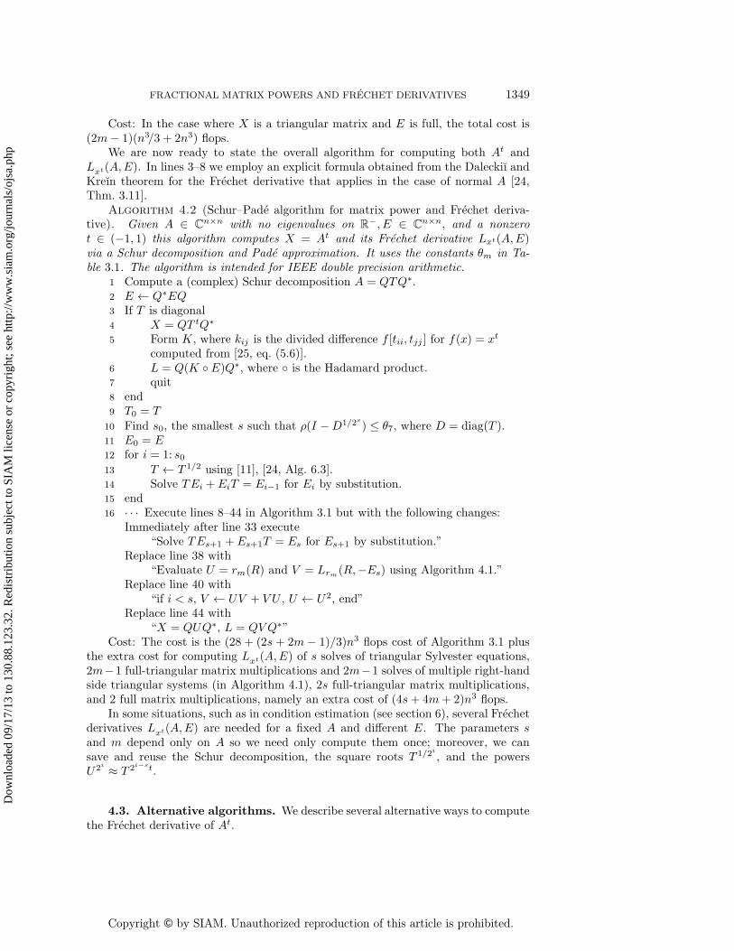
Algorithm 4.2 (Schur–Pade algorithm for matrix power and Frechet deriva-tive). Given A ∈ Cn×n with no eigenvalues on R−, E ∈ Cn×n, and a nonzerot ∈ (−1, 1) this algorithm computes X = At and its Frechet derivative Lxt(A,E)via a Schur decomposition and Pade approximation. It uses the constants θm in Ta-ble 3.1. The algorithm is intended for IEEE double precision arithmetic.

1 Compute a (complex) Schur decomposition A = QTQ∗.2 E ← Q∗EQ3 If T is diagonal4 X = QT tQ∗

5 Form K, where kij is the divided difference f [tii, tjj ] for f(x) = xt

computed from [25, eq. (5.6)].6 L = Q(K ◦ E)Q∗, where ◦ is the Hadamard product.7 quit8 end9 T0 = T

10 Find s0, the smallest s such that ρ(I −D1/2s) ≤ θ7, where D = diag(T ).11 E0 = E12 for i = 1: s013 T ← T 1/2 using [11], [24, Alg. 6.3].14 Solve TEi + EiT = Ei−1 for Ei by substitution.15 end16 · · · Execute lines 8–44 in Algorithm 3.1 but with the following changes:

Immediately after line 33 execute“Solve TEs+1 + Es+1T = Es for Es+1 by substitution.”

Replace line 38 with“Evaluate U = rm(R) and V = Lrm(R,−Es) using Algorithm 4.1.”

Replace line 40 with“if i < s, V ← UV + V U , U ← U2, end”

Replace line 44 with“X = QUQ∗, L = QVQ∗”

Cost: The cost is the (28 + (2s + 2m− 1)/3)n3 flops cost of Algorithm 3.1 plusthe extra cost for computing Lxt(A,E) of s solves of triangular Sylvester equations,2m−1 full-triangular matrix multiplications and 2m−1 solves of multiple right-handside triangular systems (in Algorithm 4.1), 2s full-triangular matrix multiplications,and 2 full matrix multiplications, namely an extra cost of (4s+ 4m+ 2)n3 flops.

In some situations, such as in condition estimation (see section 6), several Frechetderivatives Lxt(A,E) are needed for a fixed A and different E. The parameters sand m depend only on A so we need only compute them once; moreover, we cansave and reuse the Schur decomposition, the square roots T 1/2i , and the powersU2i ≈ T 2i−st.

4.3. Alternative algorithms. We describe several alternative ways to computethe Frechet derivative of At.

Dow

nloa

ded

09/1

7/13

to 1

30.8

8.12

3.32

. Red

istr

ibut

ion

subj

ect t

o SI

AM

lice

nse

or c

opyr

ight

; see

http

://w

ww

.sia

m.o

rg/jo

urna

ls/o

jsa.

php



By applying the chain rule to the expression At = exp(t logA) we obtain [25,sect. 2]

Lxt(A,E) = tLexp

(t logA,Llog(A,E)

).

The first method evaluates this formula using the inverse scaling and squaring algo-rithm of Al-Mohy, Higham, and Relton [5] to evaluate Llog and the scaling and squar-ing algorithm of Al-Mohy and Higham [2] to evaluate Lexp. Both of these algorithmsare based on Pade approximation. The total cost, assuming a Schur decompositionis initially computed and used for both the Llog and Lexp computations and thatthe maximal Pade degree is chosen in each algorithm, is about (68 2

3 + 73 (s1 + s2))n

3

flops, where s1 and s2 are the scaling parameters for the Llog and Lexp computations,respectively. This is to be compared with (62 1

3 + 4 23s)n

3 flops for Algorithm 4.2, andsince s will be of similar size to s1 these two approaches will be of broadly similarcost.

A second method is based on the property, for arbitrary f [24, eq. (3.16)],

(4.10) f

([A E0 A

])=

[f(A) Lf(A,E)0 f(A)

],

which shows that by applying Algorithm 3.1 to the 2n× 2n matrix [A E0 A ] we obtain

At and Lxt(A,E) simultaneously. This method has two drawbacks. First, it has eighttimes the cost and four times the storage requirement of Algorithm 3.1 (both of whichcan be reduced by exploiting the block triangular structure). Second, since Lf(A,E)is linear in E the norm of E should not affect an algorithm for computing Lf(A,E),but Algorithm 3.1 applied to [A E

0 A ] will be affected by ‖E‖ and the best way to scaleE is not clear.

The other approaches that we consider are applicable only when q = 1/t is aninteger. The problem is then to compute the Frechet derivative for the matrix qthroot. This can be done by exploring the relation [24, Thm. 3.5]

(4.11) Lxq (A1/q, Lx1/q(A,E)) = E.

Since Lxq (X,E) =∑q

j=1Xj−1EXq−j , L

x1/q(A,E) can be obtained by solving the

generalized Sylvester equation∑q

j=1(A1/q)j−1Y (A1/q)q−j = E for Y . An explicit for-

mula expressing the solution of the more general equation∑m

i=1Am−iXBi = Y as an

infinite integral is given by Bhatia and Uchiyama [9]. However, currently no efficientalgorithm is known for solving this equation. Another way to compute Lx1/q(A,E) isproposed by Cardoso [13]. The idea is first to write the Frechet derivative Lxq(A,E)in terms of the solution of a set of q recursive Sylvester equations and then reversethe procedure (in view of (4.11)) to get L

x1/q . The matrix A1/q must be computed bysome other method before applying this procedure. To save computation in solvingthe Sylvester equations, an initial Schur decomposition is used, which makes the co-efficients of the Sylvester equations triangular. This method costs (4q + 31 1

3 )n3 flops

plus the cost of computing A1/q and always requires complex arithmetic, even whenA and E are real. Recall that the extra cost in Algorithm 4.2 in addition to that forcomputing At is (4s + 4m+ 2)n3 flops. The values of of q, s, and m depend on theproblem but m ≤ 7, so Cardoso’s algorithm will be competitive in cost only if q ≤ s.

Another method for the qth root case is proposed by Cardoso [14], who appliesthe repeated trapezium rule to an integral representation of the Frechet derivative.This method is competitive in cost only when low accuracy is required (relative errors

Dow

nloa

ded

09/1

7/13

to 1

30.8

8.12

3.32

. Red

istr

ibut

ion

subj

ect t

o SI

AM

lice

nse

or c

opyr

ight

; see

http

://w

ww

.sia

m.o

rg/jo

urna

ls/o

jsa.

php



≥ u1/2, say), and its cost increases rough linearly with q, so we will not consider itfurther.

5. Algorithm for real data. In the case where A and E are real both At

and Lxt(A,E) are real, so an algorithm that avoids complex arithmetic is desired toincrease the efficiency of the computation and guarantee a real result in floating pointarithmetic. We summarize the changes that can be made to Algorithms 4.1 and 4.2so that they work entirely in real arithmetic for real inputs.

1. Use the real Schur decomposition instead of the Schur decomposition.2. Compute real square roots of real quasi-triangular matrices using the recur-

rence of Higham [23], [24, Alg. 6.7].3. Instead of updating the diagonal and the first superdiagonal elements before

the squaring stage by using an explicit formula for the tth power of a 2× 2 triangularmatrix, update the (full) 2× 2 diagonal blocks. Assume the 2× 2 diagonal blocks areof the form

B =

[a bc a

]

with bc < 0, which is the case when the real Schur decomposition is computed byMATLAB. Then B has eigenvalues λ± = a ± iβ, where β = (−bc)1/2. Let θ =arg(λ+) ∈ (0, π) and r = |λ+|. It can be shown that

Bt =rt

β

[β cos(tθ) b sin(tθ)c sin(tθ) β cos(tθ)

],

which can be evaluated to high relative accuracy as long as we are able to compute θ,cos, and sin accurately. The explicit formula for 2× 2 triangular matrices can still beused to update the first superdiagonal elements when two or more successive 1 × 1diagonal blocks are found.

With these changes we will gain a halving of the storage required for interme-diate matrices and an approximate halving of the operation count measured in realarithmetic operations. Fortran experiments reported in [5] with the inverse scalingand squaring algorithm for the matrix logarithm show that use of the real instead ofcomplex Schur form halves the run time, and the same will be true here since exactlythe same computational kernels are used.

6. Condition number estimation. From (1.2) and (1.3) it is clear that theessential task in computing or estimating the condition number is to compute orestimate the norm ‖Lxt(A)‖ of the Frechet derivative.

Denoting by vec the operator that stacks the columns of a matrix into one longvector, for a general f we have vec(Lf (A,Z)) = Kf(A)z, where z = vec(Z), for a

certain matrix Kf (A) ∈ Cn2×n2

called the Kronecker representation of the Frechetderivative. Moreover [24, Lem. 3.18],

(6.1)‖Lf(A)‖1

n≤ ‖Kf(A)‖1 ≤ n‖Lf(A)‖1.

We will therefore apply the block matrix 1-norm estimation algorithm of [28] toKxt(A), which requires the computation of Kxt(A)y and Kxt(A)∗z for given vectorsy and z. In order to avoid forming the n2 × n2 matrix Kxt(A) we compute Kxt(A)yas vec(Lxt(A, Y )), where vec(Y ) = y. How to compute Kxt(A)∗z is less clear. Thefollowing results provide an answer for a general function f .

Dow

nloa

ded

09/1

7/13

to 1

30.8

8.12

3.32

. Red

istr

ibut

ion

subj

ect t

o SI

AM

lice

nse

or c

opyr

ight

; see

http

://w

ww

.sia

m.o

rg/jo

urna

ls/o

jsa.

php



Our analysis makes use of the adjoint L f of the Frechet derivative Lf , which isdefined by the condition

(6.2) 〈Lf (A,G), H〉 = 〈G,L f (A,H)〉for all G,H ∈ Cn×n, where 〈X,Y 〉 = trace(Y ∗X) = vec(Y )∗vec(X).

Lemma 6.1. Kf (A)∗vec(H) = vec(L f (A,H)).

Proof. We have 〈Lf (A,G), H〉 = vec(H)∗vec(Lf(A,G)) = vec(H)∗Kf (A)vec(G)and 〈G,L f (A,H)〉 = vec(L f (A,H))∗vec(G). By the definition (6.2) of adjoint these

expressions are equal for all G and so vec(H)∗Kf(A) = vec(L f (A,H))∗, which yieldsthe result.

Lemma 6.2. Let f be 2n−1 times continuously differentiable on an open subset Dof R or C such that each connected component of D is closed under conjugation, andsuppose that f(A)∗ = f(A∗) for all A ∈ C

n×n with spectrum in D, where f(z) := f(z).Then

(6.3) L f (A,E) = Lf (A∗, E) = Lf(A,E

∗)∗.

Proof. Suppose, first, that f has the form f(x) = αxk, so that Lf (A,G) =

α∑k

i=1Ai−1GAk−i. Then

〈Lf (A,G), H〉 = trace

(H∗α

k∑i=1

Ai−1GAk−i

)

= trace

(α

k∑i=1

Ak−iH∗Ai−1G

)

=

⟨G,α

k∑i=1

(A∗)i−1H(A∗)k−i

⟩

= 〈G,Lf (A∗, H)〉,

and so L f (A,H) = Lf (A∗, H), which is the first equality in (6.3). By the linearity of

Lf it follows that this equality holds for any polynomial. Finally, the equality holdsfor all f satisfying the conditions of the theorem because the Frechet derivative of fis the same as that of the polynomial that interpolates f and its derivatives at thezeros of the characteristic polynomial of diag(A,A) [24, Thm. 3.7], [29, Thm. 6.6.14].

Let g = f . By the definition of Frechet derivative, Lg(A,E) = g(A+E)− g(A)+o(‖E‖). Taking the conjugate transpose gives Lg(A,E)∗ = g(A + E)∗ − g(A)∗ +o(‖E‖) = g(A∗ +E∗)− g(A∗) + o(‖E‖) = Lg(A

∗, E∗) + o(‖E‖), and by the linearityof the Frechet derivative it follows that Lg(A,E)∗ = Lg(A

∗, E∗), which is equivalentto the second equality in (6.3).

If f is n− 1 times continuously differentiable on D (so that f(A) is a continuousmatrix function on the set of matrices with spectrum in D [24, Thm. 1.19]), thenf(A∗) = f(A)∗ for all A with spectrum in D is equivalent to f ≡ f [26, Proof ofThm. 3.2]. Some other equivalent conditions for f(A∗) = f(A)∗ are given in [24,Thm. 1.18], [26, Thm. 3.2].

Combining Lemmas 6.1 and 6.2 gives Kf(A)∗vec(H) = vec(Lf (A,H

∗)∗). For ourfunction f(x) = xt we have f ≡ f and so to implement the condition estimation wejust need to evaluate Lf(A).

Dow

nloa

ded

09/1

7/13

to 1

30.8

8.12

3.32

. Red

istr

ibut

ion

subj

ect t

o SI

AM

lice

nse

or c

opyr

ight

; see

http

://w

ww

.sia

m.o

rg/jo

urna

ls/o

jsa.

php



7. Numerical experiments. Our numerical experiments were carried out inMATLAB R2012b in IEEE double precision arithmetic. We use the same set of 45test matrices that was used in [25] to test the original Schur–Pade algorithm. Thisset includes a selection of 10 × 10 nonsingular matrices taken from the MATLABgallery function and from the Matrix Computation Toolbox [22]. Any matrix foundto have an eigenvalue on R− was squared; if it still had an eigenvalue on R− it wasdiscarded. We report experiments using the matrices in the test set and their complexSchur factors T . Our previous experience [2], [5], [25] is that for methods that beginwith a reduction to Schur form, differences in accuracy between different methods aregreater when the original matrix is triangular, as errors in the transformations to andfrom Schur form are avoided.

We test each matrix with each of the 14 t-values in the vector constructed by

v = [ 1/52 1/12 1/3 1/2 ] , v = [ v 1− v(1 : 3) ] , v = [ v −v ] .

For the computation of At alone we tested three algorithms:1. SPade: Algorithm 3.1.2. SPade-real: the real version of Algorithm 3.1, as described in section 5.3. SPade-old: the original Schur–Pade algorithm [25, Alg. 5.1], which is based

on the error analysis in Theorem 2.1 expressed in terms of ‖A‖.Relative errors are measured in the 1-norm. To compute the “exact” At we runpowerm [25, Fig. 8.1] (which uses the eigendecomposition of A) in 300 digit precisionwith the VPA arithmetic of the Symbolic Math Toolbox, but we subject A to a randomperturbation of relative norm 10−150 in order to ensure it is diagonalizable, followingthe approximate diagonalization approach of Davis [15]. All errors are postprocessedusing the transformation in [17] to lessen the influence of tiny relative errors on theperformance profiles.

For the Frechet derivative Lxt(A,E), we tested six algorithms:1. SPade-Fre: Algorithm 4.2.2. SPade-Fre-real: the real version of Algorithm 4.2, as described in section 5.3. SPade-Fre-mod: Algorithm 4.2 modified so as to call SPade-old instead of

SPade.4. explog-Fre: reduction to Schur form T = Q∗AQ followed by evaluation

of Lxt(A,E) = tQLexp(t logT, Llog(T,Q∗EQ))Q∗ by the inverse scaling and

squaring method for the Frechet derivative of the logarithm [5] and the scalingand squaring method for the Frechet derivative of the exponential [2].

5. SPade-2by2: SPade applied to the block 2× 2 matrix in (4.10).6. rootm-Fre (applied when t = 1/q for some integer q): reduction to Schur

form T with T 1/q computed by SPade and Lx1/q(T,Q∗EQ) computed by [13,Alg. 3.5].

To obtain the “exact” Frechet derivative we apply the same approach as aboveto (4.10).

We note that for an efficient implementation, which is not our concern here, it isimportant to implement carefully the computation of square roots of (quasi-) trian-gular matrices and the solution of (quasi-) triangular Sylvester equations. Efficientblocked and recursive ways to carry out these operations are described by Deadman,Higham, and Ralha [16] and Jonsson and Kagstrom [32], respectively.

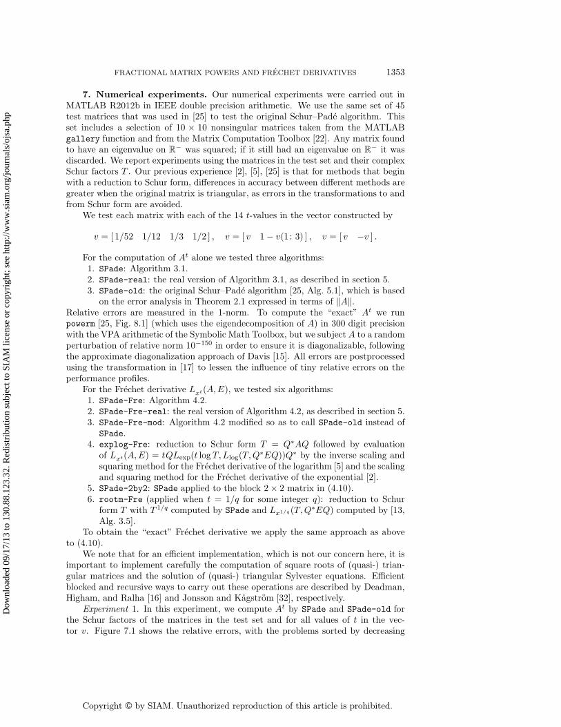
Experiment 1. In this experiment, we compute At by SPade and SPade-old forthe Schur factors of the matrices in the test set and for all values of t in the vec-tor v. Figure 7.1 shows the relative errors, with the problems sorted by decreasing

Dow

nloa

ded

09/1

7/13

to 1

30.8

8.12

3.32

. Red

istr

ibut

ion

subj

ect t

o SI

AM

lice

nse

or c

opyr

ight

; see

http

://w

ww

.sia

m.o

rg/jo

urna

ls/o

jsa.

php



0 100 200 300 400 500

10−17

10−16

10−15

10−14

10−13

SPadeSPade−old

Fig. 7.1. Experiment 1: relative errors in At for a selection of 10× 10 triangular matrices andseveral t.

1 1.5 2 2.5 3 3.5 4 4.5 50.7

0.75

0.8

0.85

0.9

0.95

1

α

π

SPadeSPade−old

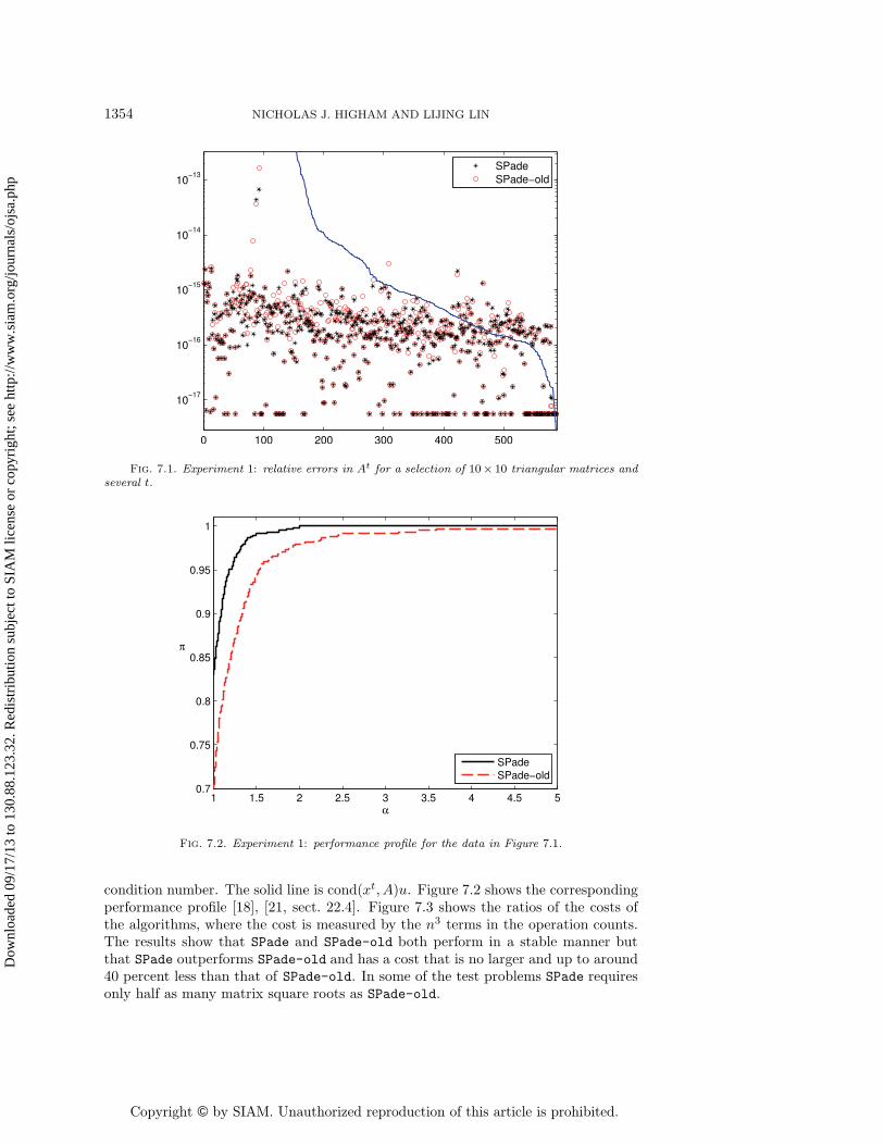
Fig. 7.2. Experiment 1: performance profile for the data in Figure 7.1.

condition number. The solid line is cond(xt, A)u. Figure 7.2 shows the correspondingperformance profile [18], [21, sect. 22.4]. Figure 7.3 shows the ratios of the costs ofthe algorithms, where the cost is measured by the n3 terms in the operation counts.The results show that SPade and SPade-old both perform in a stable manner butthat SPade outperforms SPade-old and has a cost that is no larger and up to around40 percent less than that of SPade-old. In some of the test problems SPade requiresonly half as many matrix square roots as SPade-old.

Dow

nloa

ded

09/1

7/13

to 1

30.8

8.12

3.32

. Red

istr

ibut

ion

subj

ect t

o SI

AM

lice

nse

or c

opyr

ight

; see

http

://w

ww

.sia

m.o

rg/jo

urna

ls/o

jsa.

php



0 100 200 300 400 5000.5

0.6

0.7

0.8

0.9

1

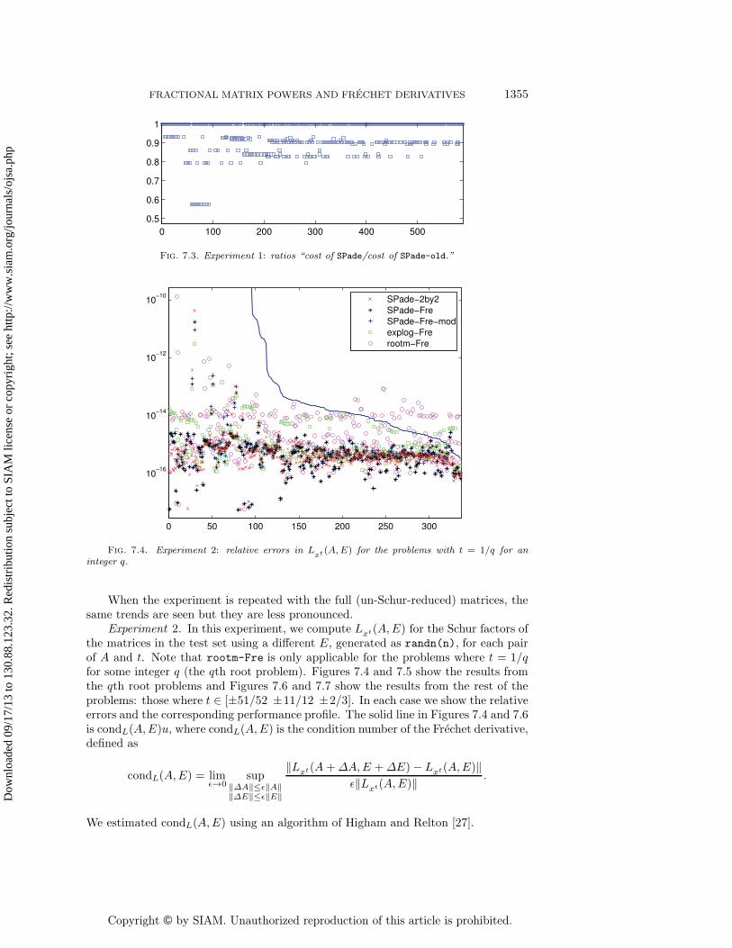
Fig. 7.3. Experiment 1: ratios “cost of SPade/cost of SPade-old.”

0 50 100 150 200 250 300

10−16

10−14

10−12

10−10

SPade−2by2SPade−FreSPade−Fre−modexplog−Frerootm−Fre

Fig. 7.4. Experiment 2: relative errors in Lxt(A,E) for the problems with t = 1/q for an

integer q.

When the experiment is repeated with the full (un-Schur-reduced) matrices, thesame trends are seen but they are less pronounced.

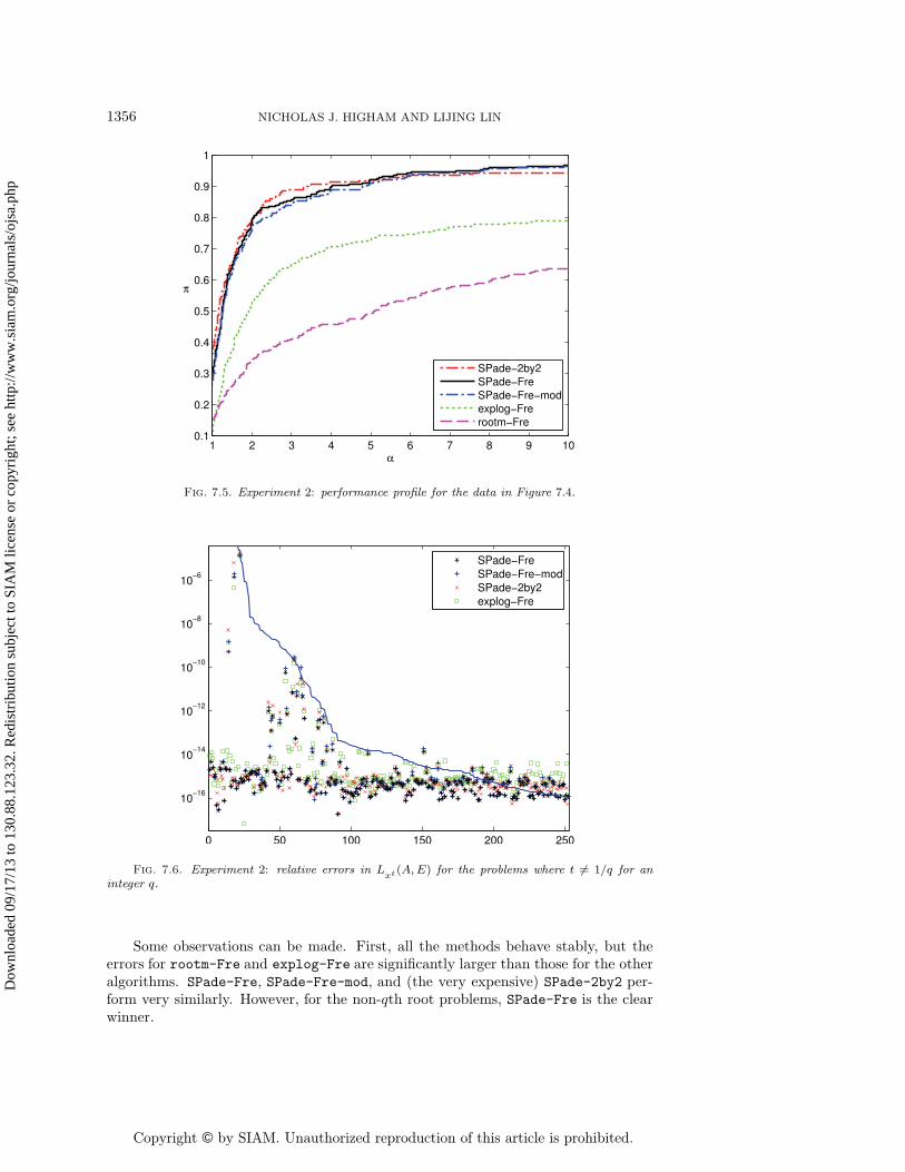
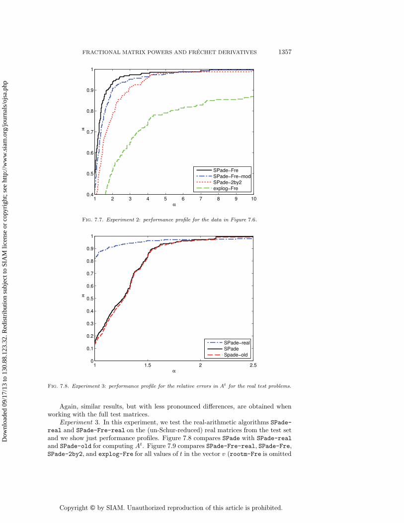
Experiment 2. In this experiment, we compute Lxt(A,E) for the Schur factors ofthe matrices in the test set using a different E, generated as randn(n), for each pairof A and t. Note that rootm-Fre is only applicable for the problems where t = 1/qfor some integer q (the qth root problem). Figures 7.4 and 7.5 show the results fromthe qth root problems and Figures 7.6 and 7.7 show the results from the rest of theproblems: those where t ∈ [±51/52 ±11/12 ±2/3]. In each case we show the relativeerrors and the corresponding performance profile. The solid line in Figures 7.4 and 7.6is condL(A,E)u, where condL(A,E) is the condition number of the Frechet derivative,defined as

condL(A,E) = limε→0

sup‖ΔA‖≤ε‖A‖‖ΔE‖≤ε‖E‖

‖Lxt(A+ΔA,E +ΔE)− Lxt(A,E)‖ε‖Lxt(A,E)‖ .

We estimated condL(A,E) using an algorithm of Higham and Relton [27].

Dow

nloa

ded

09/1

7/13

to 1

30.8

8.12

3.32

. Red

istr

ibut

ion

subj

ect t

o SI

AM

lice

nse

or c

opyr

ight

; see

http

://w

ww

.sia

m.o

rg/jo

urna

ls/o

jsa.

php



1 2 3 4 5 6 7 8 9 100.1

0.2

0.3

0.4

0.5

0.6

0.7

0.8

0.9

1

α

π

SPade−2by2SPade−FreSPade−Fre−modexplog−Frerootm−Fre


0 50 100 150 200 250

10−16

10−14

10−12

10−10

10−8

10−6

SPade−FreSPade−Fre−modSPade−2by2explog−Fre

Fig. 7.6. Experiment 2: relative errors in Lxt(A,E) for the problems where t �= 1/q for an

integer q.

Some observations can be made. First, all the methods behave stably, but theerrors for rootm-Fre and explog-Fre are significantly larger than those for the otheralgorithms. SPade-Fre, SPade-Fre-mod, and (the very expensive) SPade-2by2 per-form very similarly. However, for the non-qth root problems, SPade-Fre is the clearwinner.

Dow

nloa

ded

09/1

7/13

to 1

30.8

8.12

3.32

. Red

istr

ibut

ion

subj

ect t

o SI

AM

lice

nse

or c

opyr

ight

; see

http

://w

ww

.sia

m.o

rg/jo

urna

ls/o

jsa.

php



1 2 3 4 5 6 7 8 9 100.4

0.5

0.6

0.7

0.8

0.9

1

α

π

SPade−FreSPade−Fre−modSPade−2by2explog−Fre


1 1.5 2 2.50

0.1

0.2

0.3

0.4

0.5

0.6

0.7

0.8

0.9

1

α

π

SPade−realSPadeSpade−old

Fig. 7.8. Experiment 3: performance profile for the relative errors in At for the real test problems.

Again, similar results, but with less pronounced differences, are obtained whenworking with the full test matrices.

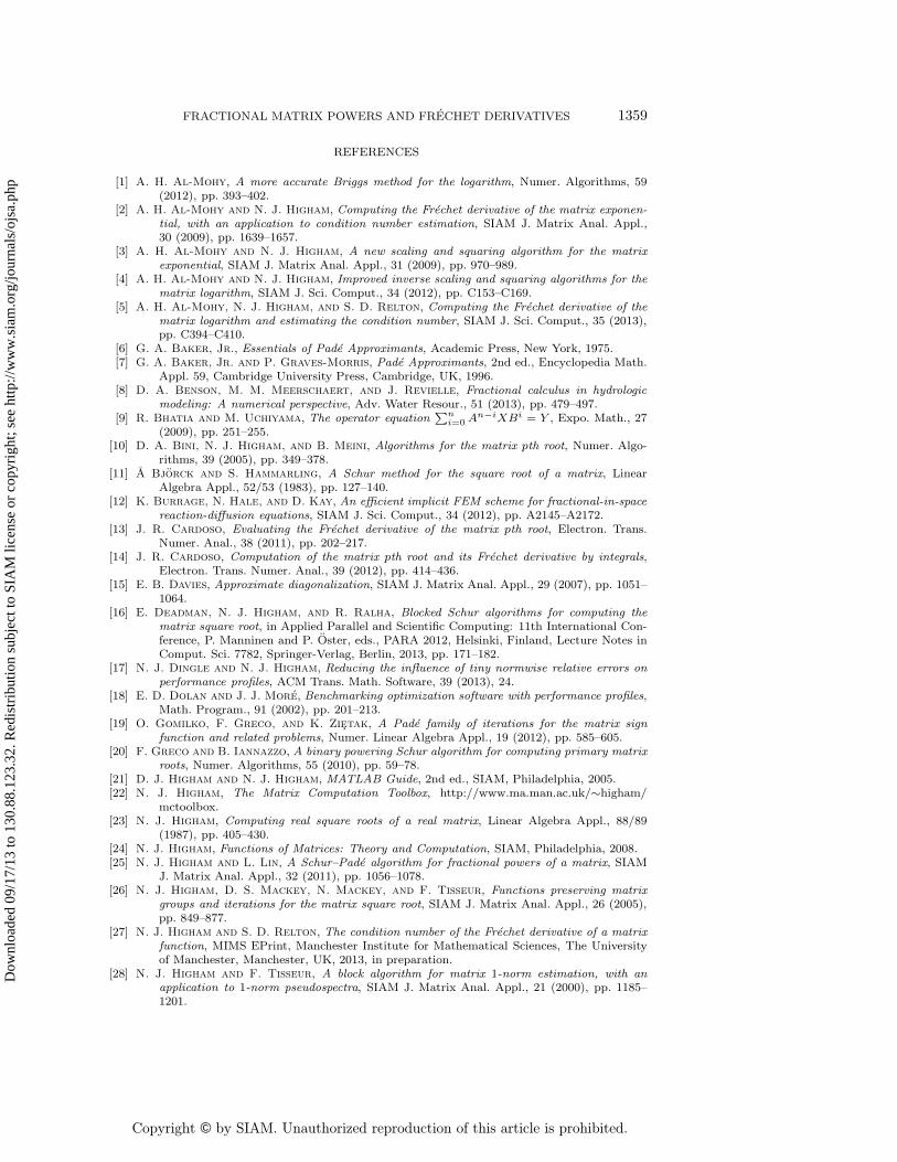
Experiment 3. In this experiment, we test the real-arithmetic algorithms SPade-real and SPade-Fre-real on the (un-Schur-reduced) real matrices from the test setand we show just performance profiles. Figure 7.8 compares SPade with SPade-real

and SPade-old for computing At. Figure 7.9 compares SPade-Fre-real, SPade-Fre,SPade-2by2, and explog-Fre for all values of t in the vector v (rootm-Fre is omitted

Dow

nloa

ded

09/1

7/13

to 1

30.8

8.12

3.32

. Red

istr

ibut

ion

subj

ect t

o SI

AM

lice

nse

or c

opyr

ight

; see

http

://w

ww

.sia

m.o

rg/jo

urna

ls/o

jsa.

php



1 1.5 2 2.5 3 3.5 4 4.5 50

0.1

0.2

0.3

0.4

0.5

0.6

0.7

0.8

0.9

1

α

π

SPade−Fre−realSPade−FreSPade−2by2explog−Fre

Fig. 7.9. Experiment 3: performance profile for the relative errors in Lxt(A,E) for the real

test problems.

due to its poor performance in the previous experiment). For these real problems,SPade-real and SPade-Fre-real show a significant improvement in accuracy overthe algorithms working in complex arithmetic.

Finally, we mention that we used SPade-Fre with the block 1-norm estimatorto estimate the condition numbers of At with matrices in the test set and found theestimate of ‖Kxt(A)‖1 always to be within a factor 2 of the true quantity.

8. Conclusions. This work provides three main contributions.1. The improved Schur–Pade algorithm with sharper underlying error analysis.

Our experiments show that the improved algorithm is more accurate and often moreefficient (by up to 40 percent for our test problems) than the original algorithm of [25].

2. An extension of the improved Schur–Pade algorithm that also computes theFrechet derivative. We have shown this algorithm to be superior in accuracy to andat least as efficient as alternative techniques. The fact that the Frechet derivativecomputation in Algorithm 4.2 is based on an error bound that is strictly valid onlyfor the At computation itself (see section 4.1) does not affect the accuracy of thecomputed Frechet derivatives in our experiments (as was found analogously for thematrix logarithm in [5]).

3. The real arithmetic versions of the improved and extended algorithms for realdata. These bring a significant improvement in accuracy over the complex versions,run at twice the speed, and need only half the intermediate storage.

Finally, it is worth emphasizing that when 1/t = q ∈ Z, our algorithms are verycompetitive with algorithms specialized to the matrix qth root problem, as is shownhere, in further tests we have conducted that are not reported here, and in [25],[30]. Moreover, our algorithms have an operation count independent of q, unlike mostalgorithms for the qth root problem [10], [20], [24, Chap. 7], [30], and this is significantfor applications requiring a large q, such as the optic applications in [34] in which qcan be as large as 105.

Dow

nloa

ded

09/1

7/13

to 1

30.8

8.12

3.32

. Red

istr

ibut

ion

subj

ect t

o SI

AM

lice

nse

or c

opyr

ight

; see

http

://w

ww

.sia

m.o

rg/jo

urna

ls/o

jsa.

php



REFERENCES

[1] A. H. Al-Mohy, A more accurate Briggs method for the logarithm, Numer. Algorithms, 59(2012), pp. 393–402.

[2] A. H. Al-Mohy and N. J. Higham, Computing the Frechet derivative of the matrix exponen-tial, with an application to condition number estimation, SIAM J. Matrix Anal. Appl.,30 (2009), pp. 1639–1657.

[3] A. H. Al-Mohy and N. J. Higham, A new scaling and squaring algorithm for the matrixexponential, SIAM J. Matrix Anal. Appl., 31 (2009), pp. 970–989.

[4] A. H. Al-Mohy and N. J. Higham, Improved inverse scaling and squaring algorithms for thematrix logarithm, SIAM J. Sci. Comput., 34 (2012), pp. C153–C169.

[5] A. H. Al-Mohy, N. J. Higham, and S. D. Relton, Computing the Frechet derivative of thematrix logarithm and estimating the condition number, SIAM J. Sci. Comput., 35 (2013),pp. C394–C410.

[6] G. A. Baker, Jr., Essentials of Pade Approximants, Academic Press, New York, 1975.[7] G. A. Baker, Jr. and P. Graves-Morris, Pade Approximants, 2nd ed., Encyclopedia Math.

Appl. 59, Cambridge University Press, Cambridge, UK, 1996.[8] D. A. Benson, M. M. Meerschaert, and J. Revielle, Fractional calculus in hydrologic

modeling: A numerical perspective, Adv. Water Resour., 51 (2013), pp. 479–497.[9] R. Bhatia and M. Uchiyama, The operator equation

∑ni=0 A

n−iXBi = Y , Expo. Math., 27(2009), pp. 251–255.

[10] D. A. Bini, N. J. Higham, and B. Meini, Algorithms for the matrix pth root, Numer. Algo-rithms, 39 (2005), pp. 349–378.

[11] A Bjorck and S. Hammarling, A Schur method for the square root of a matrix, LinearAlgebra Appl., 52/53 (1983), pp. 127–140.

[12] K. Burrage, N. Hale, and D. Kay, An efficient implicit FEM scheme for fractional-in-spacereaction-diffusion equations, SIAM J. Sci. Comput., 34 (2012), pp. A2145–A2172.

[13] J. R. Cardoso, Evaluating the Frechet derivative of the matrix pth root, Electron. Trans.Numer. Anal., 38 (2011), pp. 202–217.

[14] J. R. Cardoso, Computation of the matrix pth root and its Frechet derivative by integrals,Electron. Trans. Numer. Anal., 39 (2012), pp. 414–436.

[15] E. B. Davies, Approximate diagonalization, SIAM J. Matrix Anal. Appl., 29 (2007), pp. 1051–1064.

[16] E. Deadman, N. J. Higham, and R. Ralha, Blocked Schur algorithms for computing thematrix square root, in Applied Parallel and Scientific Computing: 11th International Con-ference, P. Manninen and P. Oster, eds., PARA 2012, Helsinki, Finland, Lecture Notes inComput. Sci. 7782, Springer-Verlag, Berlin, 2013, pp. 171–182.

[17] N. J. Dingle and N. J. Higham, Reducing the influence of tiny normwise relative errors onperformance profiles, ACM Trans. Math. Software, 39 (2013), 24.

[18] E. D. Dolan and J. J. More, Benchmarking optimization software with performance profiles,Math. Program., 91 (2002), pp. 201–213.

[19] O. Gomilko, F. Greco, and K. Zietak, A Pade family of iterations for the matrix signfunction and related problems, Numer. Linear Algebra Appl., 19 (2012), pp. 585–605.

[20] F. Greco and B. Iannazzo, A binary powering Schur algorithm for computing primary matrixroots, Numer. Algorithms, 55 (2010), pp. 59–78.

[21] D. J. Higham and N. J. Higham, MATLAB Guide, 2nd ed., SIAM, Philadelphia, 2005.[22] N. J. Higham, The Matrix Computation Toolbox, http://www.ma.man.ac.uk/∼higham/

mctoolbox.[23] N. J. Higham, Computing real square roots of a real matrix, Linear Algebra Appl., 88/89

(1987), pp. 405–430.[24] N. J. Higham, Functions of Matrices: Theory and Computation, SIAM, Philadelphia, 2008.[25] N. J. Higham and L. Lin, A Schur–Pade algorithm for fractional powers of a matrix, SIAM

J. Matrix Anal. Appl., 32 (2011), pp. 1056–1078.[26] N. J. Higham, D. S. Mackey, N. Mackey, and F. Tisseur, Functions preserving matrix

groups and iterations for the matrix square root, SIAM J. Matrix Anal. Appl., 26 (2005),pp. 849–877.

[27] N. J. Higham and S. D. Relton, The condition number of the Frechet derivative of a matrixfunction, MIMS EPrint, Manchester Institute for Mathematical Sciences, The Universityof Manchester, Manchester, UK, 2013, in preparation.

[28] N. J. Higham and F. Tisseur, A block algorithm for matrix 1-norm estimation, with anapplication to 1-norm pseudospectra, SIAM J. Matrix Anal. Appl., 21 (2000), pp. 1185–1201.

Dow

nloa

ded

09/1

7/13

to 1

30.8

8.12

3.32

. Red

istr

ibut

ion

subj

ect t

o SI

AM

lice

nse

or c

opyr

ight

; see

http

://w

ww

.sia

m.o

rg/jo

urna

ls/o

jsa.

php



[29] R. A. Horn and C. R. Johnson, Topics in Matrix Analysis, Cambridge University Press,Cambridge, UK, 1991.

[30] B. Iannazzo and C. Manasse, A Schur logarithmic algorithm for fractional powers of matri-ces, SIAM J. Matrix Anal. Appl., 34 (2013), pp. 794–813.

[31] M. Ilic, I. W. Turner, and V. Anh, A numerical solution using an adaptively preconditionedLanczos method for a class of linear systems related with the fractional Poisson equation,J. Appl. Math. Stoch. Anal., 2008, 104525.

[32] I. Jonsson and B. Kagstrom, Recursive blocked algorithms for solving triangular systems—Part I: One-sided and coupled Sylvester-type matrix equations, ACM Trans. Math. Soft-ware, 28 (2002), pp. 392–415.

[33] C. S. Kenney and A. J. Laub, Pade error estimates for the logarithm of a matrix, Internat.J. Control, 50 (1989), pp. 707–730.

[34] H. D. Noble and R. A. Chipman, Mueller matrix roots algorithm and computational consid-erations, Opt. Express, 20 (2012), pp. 17–31.

Dow

nloa

ded

09/1

7/13

to 1

30.8

8.12

3.32

. Red

istr

ibut

ion

subj

ect t

o SI

AM

lice

nse

or c

opyr

ight

; see

http

://w

ww

.sia

m.o

rg/jo

urna

ls/o

jsa.

php

Documents

An Improved Schur–Pade Algorithm for Fractional Powers of ...eprints.ma.man.ac.uk/2021/01/covered/MIMS_ep2013_1.pdf · An Improved Schur–Pade Algorithm for Fractional Powers of