Embed Size (px)
Citation preview
AN IMPROVED MICROWAVE RADIATIVE TRANSFER MODEL FOR OCEAN EMISSIVITY AT HURRICANE FORCE SURFACE WIND SPEED
by
SALEM FAWWAZ EL-NIMRI B.S. Princess Sumaya University for Technology, 2004
A thesis submitted in partial fulfillment of the requirements for the degree of Master of Science
in the School of Electrical Engineering and Computer Science in the College of Engineering and Computer Science
at the University of Central Florida Orlando, Florida
Summer Term 2006
© 2006 Salem Fawwaz EL-Nimri
ii
ABSTRACT
An electromagnetic model for predicting the microwave blackbody emission from the
ocean surface under the forcing of strong surface winds in hurricanes is being developed. This
ocean emissivity model will be incorporated into a larger radiative transfer model used to infer
ocean surface wind speed and rain rate in hurricanes from remotely sensed radiometric
brightness temperature. The model development is based on measurements obtained with the
Stepped Frequency Microwave Radiometer (SFMR), which routinely flys on the National
Oceanic and Atmospheric Administration’s hurricane hunter aircraft. This thesis presents the
methods used in the wind speed model development and validation results for wind speeds up to
70 m/sec.
The ocean emissivity model relates changes in measured C-band radiometric brightness
temperatures to physical changes in the ocean surface. These surface modifications are the result
of the drag of surface winds that roughen the sea surface, produce waves, and create white caps
and foam from the breaking waves. SFMR brightness temperature measurements from hurricane
flights and independent measurements of surface wind speed are used to define empirical
relationships between microwave brightness temperature and surface wind speed. The wind
speed model employs statistical regression techniques to develop a physics-based ocean
emissivity model dependent on geophysical parameters, such as wind speed and sea surface
temperature, and observational parameters, such as electromagnetic frequency, electromagnetic
polarization, and incidence angle.
iii
In The Memory of My Father
Who made me believe that leaders are made…not born
Eng. Fawwaz Methyeb EL-Nimri
To the hands that rocked my cradle
To the person who believed in me
To you… MOM
iv
ACKNOWLEDGMENTS
I would like to thank my advisor, Dr. Linwood Jones and my committee members, Mr.
James Johnson, Dr. Takis Kasparis and Dr. Stephan Watson, for their guidance, advice, interests
and time. I would like to thank my parents for their love, encouragement and support that carried
me through my whole life and me stronger each day along the way. Also, I am thankful to my
team members for their assistance especially Ruba Amarin, Suleiman Al-Sweiss and Liang
Hong.
I want to give my special thanks to Mr. and Mrs. Johnson for their help and tremendous
love throughout my graduate school and this project. Last but not least I would like to thank all
of my friends for their encouragements.
This work was accomplished with the help of NOAA’s through Dr. Peter Black and Mr.
Eric Uhlhorn.
v
TABLE OF CONTENTS
LIST OF FIGURES ..................................................................................................................... viii
LIST OF TABLES.......................................................................................................................... x
LIST OF ACRONYMS/ABBREVIATIONS................................................................................ xi
CHAPTER 1 : INTRODUCTION .............................................................................................. 1
1.1 Thesis Objective.............................................................................................................. 1
1.2 Microwave Remote Sensing ........................................................................................... 2
1.2.1 Rayleigh-Jeans Law................................................................................................ 3
1.2.2 Radiative Transfer Theory ...................................................................................... 6
1.3 Ocean Surface Wind Speed Remote Sensing ................................................................. 9
1.3.1 Satellite Radiometers .............................................................................................. 9
1.3.2 SFMR Measurements............................................................................................ 11
CHAPTER 2 : SEA SURFACE EMISSION ............................................................................ 13
2.1 Physical Principles ........................................................................................................ 13
2.1.1 Fresnel Voltage Reflection Coefficient ................................................................ 14
2.1.2 Surface Emissivity ................................................................................................ 17
2.1.3 Dielectric Constant of Sea Water.......................................................................... 18
2.2 Sea Surface Emissivity ................................................................................................. 21
2.2.1 Smooth Water Emissivity ..................................................................................... 21
2.2.2 Rough Sea Surface Emissivity Model .................................................................. 22
2.3 Sea Foam....................................................................................................................... 25
2.3.1 Effect of Foam on Oceanic Emission ................................................................... 25
vi
2.3.2 Emissivity of Foam............................................................................................... 26
2.3.3 Foam Fraction - Wind Speed Dependence ........................................................... 27
CHAPTER 3 : WIND SPEED EMISSIVITY MODEL DEVELOPMENT............................. 29
3.1 Existing Wind Speed Emissivity Models ..................................................................... 29
3.1.1 Near-Nadir Models ............................................................................................... 30
3.1.2 Off-Nadir Models.................................................................................................. 33
3.2 CFRSL High Wind Speed Emissivity Model ............................................................... 36
3.2.1 Near Nadir High Wind Speed Modeling .............................................................. 37
3.2.2 Off-Nadir High Wind Speed Modeling: ............................................................... 41
CHAPTER 4 : EMISSIVITY MODEL VALIDATIONS......................................................... 50
4.1 SFMR Comparisons...................................................................................................... 50
4.2 Error Estimates.............................................................................................................. 55
CHAPTER 5 : CONCLUSION................................................................................................. 63
APPENDIX: SFMR INSTUMENT DISCRIPTION.................................................................... 66
LIST OF REFERENCES.............................................................................................................. 70
vii
LIST OF FIGURES
Figure 1.1 : Rayleigh-Jeans approximation to Plank’s law in microwave region. ......................... 5
Figure 1.2 : Simplified microwave radiative transfer over the ocean............................................. 8
Figure 1.3 : WindSat ocean surface wind speed 9-day average October, 1992............................ 10
Figure 2.1: Plane wave reflection and transmission at the air/ocean interface. ............................ 15
Figure 2.2 : Typical ocean power reflection coefficient. .............................................................. 16
Figure 2.3 : Real (upper panel) and imaginary part (lower panel) of dielectric constant for saline
and pure water....................................................................................................................... 20
Figure 2.4 : Typical sea water emissivity for 4.55 GHz. .............................................................. 22
Figure 2.5 : Smooth and rough emissivity for 4 and 7 GHz and wind speeds of zero, 5 and 10
m/sec. .................................................................................................................................... 24
Figure 3.1 : SFMR excess emissivity wind model. ...................................................................... 33
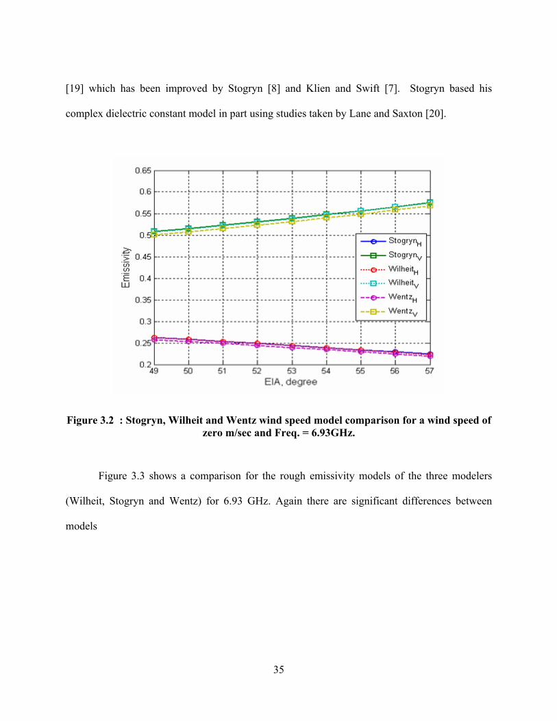
Figure 3.2 : Stogryn, Wilheit and Wentz wind speed model comparison for a wind speed of zero
m/sec and Freq. = 6.93GHz. ................................................................................................. 35
Figure 3.3 : Stogryn, Wilheit and Wentz wind speed model comparison for a wind speed of 10
m/sec and Freq. = 6.93GHz. ................................................................................................. 36
Figure 3.4 : Melville white caps coverage (WCC) measurements. .............................................. 39
Figure 3.5 : SFMR antenna pattern gain...................................................................................... 42
Figure 3.6 : SFMR antenna viewing ocean surface. ..................................................................... 43
Figure 3.7 : Plane of incidence for off-nadir Tb measurements. .................................................. 44
Figure 3.8 : Example of SFMR brightness temperature during an aircraft turn. .......................... 44
viii
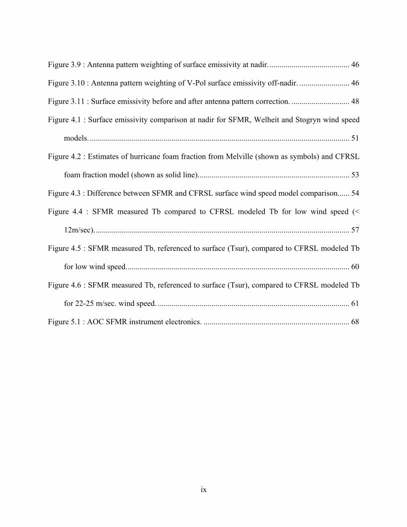
Figure 3.9 : Antenna pattern weighting of surface emissivity at nadir. ........................................ 46
Figure 3.10 : Antenna pattern weighting of V-Pol surface emissivity off-nadir. ......................... 46
Figure 3.11 : Surface emissivity before and after antenna pattern correction. ............................. 48
Figure 4.1 : Surface emissivity comparison at nadir for SFMR, Welheit and Stogryn wind speed
models. .................................................................................................................................. 51
Figure 4.2 : Estimates of hurricane foam fraction from Melville (shown as symbols) and CFRSL
foam fraction model (shown as solid line)............................................................................ 53
Figure 4.3 : Difference between SFMR and CFRSL surface wind speed model comparison...... 54
Figure 4.4 : SFMR measured Tb compared to CFRSL modeled Tb for low wind speed (<
12m/sec)................................................................................................................................ 57
Figure 4.5 : SFMR measured Tb, referenced to surface (Tsur), compared to CFRSL modeled Tb
for low wind speed................................................................................................................ 60
Figure 4.6 : SFMR measured Tb, referenced to surface (Tsur), compared to CFRSL modeled Tb
for 22-25 m/sec. wind speed. ................................................................................................ 61
Figure 5.1 : AOC SFMR instrument electronics. ......................................................................... 68
ix
LIST OF TABLES
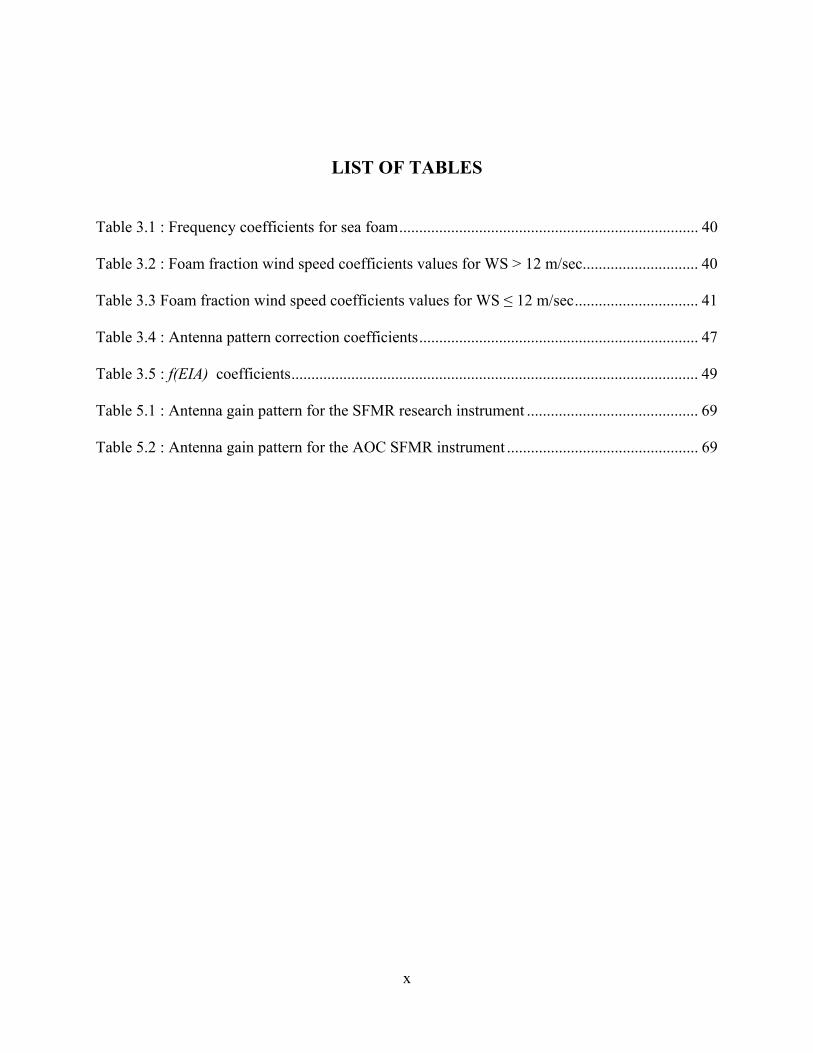
Table 3.1 : Frequency coefficients for sea foam........................................................................... 40
Table 3.2 : Foam fraction wind speed coefficients values for WS > 12 m/sec............................. 40
Table 3.3 Foam fraction wind speed coefficients values for WS ≤ 12 m/sec............................... 41
Table 3.4 : Antenna pattern correction coefficients...................................................................... 47
Table 3.5 : f(EIA) coefficients...................................................................................................... 49
Table 5.1 : Antenna gain pattern for the SFMR research instrument ........................................... 69
Table 5.2 : Antenna gain pattern for the AOC SFMR instrument ................................................ 69
x
LIST OF ACRONYMS/ABBREVIATIONS
CFRSL Central Florida Remote Sensing Lab
RTM Radiative Transfer Model
EIA Earth Incidence Angles
NOAA National Oceanic and Atmospheric Administration
NESDIS National Environmental Satellite Data and Information
Service
SFMR Stepped Frequency Microwave Radiometer
TPC NOAA Tropical Prediction Center
NHC NOAA National Hurricane Center
HRD NOAA Hurricane Research Division
WCC White Caps Coverage
HIRad Hurricane Imaging Radiometer
xi
CHAPTER 1 : INTRODUCTION
Electrical engineering microwave communications technologies contribute significantly
to environmental remote sensing. Microwaves are useful in remote sensing because of their
ability to penetrate clouds and operate day or night and in severe weather to view the earth’s
surface. Therefore, microwave sensors play an important role in providing measurements of
important atmospheric, oceanic, terrestrial, and ice environmental parameters; and they routinely
operate from aircraft and satellites to provide these valuable environmental measurements for
scientific research (e.g., global climate change) and operational utilization by federal
governmental agencies (e.g., numerical weather forecasting).
1.1 Thesis Objective
The Central Florida Remote Sensing Lab, CFRSL, is engaged in research to develop
microwave remote sensing techniques for oceanic and atmospheric applications. The CFRSL has
developed an analytical microwave radiative transfer model (RTM) that simulates passive
microwave measurements from the ocean surface. This thesis provides an important upgrade to
this RTM, by improved ocean surface wind speed modeling. The objective is to develop a
physics-based microwave RTM that characterizes the sea surface microwave blackbody
emissions for a variety of microwave instruments and measurement geometries. Developing such
a RTM will yield an accurate prediction of polarized microwave brightness temperature over a
wide range of ocean wind speeds, frequencies, and earth incidence angles (EIA). It will be useful
in engineering design studies of passive microwave remote sensing instruments and for
1
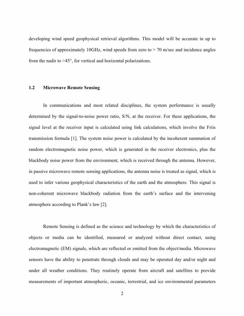
developing wind speed geophysical retrieval algorithms. This model will be accurate in up to
frequencies of approximately 10GHz, wind speeds from zero to > 70 m/sec and incidence angles
from the nadir to >45°, for vertical and horizontal polarizations.
1.2 Microwave Remote Sensing
In communications and most related disciplines, the system performance is usually
determined by the signal-to-noise power ratio, S/N, at the receiver. For these applications, the
signal level at the receiver input is calculated using link calculations, which involve the Friis
transmission formula [1]. The system noise power is calculated by the incoherent summation of
random electromagnetic noise power, which is generated in the receiver electronics, plus the
blackbody noise power from the environment, which is received through the antenna. However,
in passive microwave remote sensing applications, the antenna noise is treated as signal, which is
used to infer various geophysical characteristics of the earth and the atmosphere. This signal is
non-coherent microwave blackbody radiation from the earth’s surface and the intervening
atmosphere according to Plank’s law [2].
Remote Sensing is defined as the science and technology by which the characteristics of
objects or media can be identified, measured or analyzed without direct contact, using
electromagnetic (EM) signals, which are reflected or emitted from the object/media. Microwave
sensors have the ability to penetrate through clouds and may be operated day and/or night and
under all weather conditions. They routinely operate from aircraft and satellites to provide
measurements of important atmospheric, oceanic, terrestrial, and ice environmental parameters
2
for many applications including scientific research (e.g., global climate change) and operational
utilization by federal governmental agencies (e.g., numerical weather forecasting).
1.2.1 Rayleigh-Jeans Law
Blackbody radiation by definition refers to an object or medium which absorbs all
radiation incidents upon it and then re-radiates energy according to Planck’s radiation law. A
blackbody radiates uniformly in all directions (isotropic) with a spectral brightness as shown in
the following equation:
⎟⎟⎟
⎠
⎞
⎜⎜⎜
⎝
⎛
−=
1
12)( 5
2
kThc
e
hcSλ
λπλ (1.1)
Where:
S (λ) = blackbody energy spectral flux density, W/m3,
h = Planck’s constant = 6.63*10-34 joule sec
λ = wavelength, m
k =Boltzmann’s constant = 1.38*10-23 joule/K
T = Blackbody absolute Temperature, Kelvin
c = speed of light = 3*108 m/sec
At microwave frequencies, the Rayleigh-Jeans law is an excellent approximation to Planck’s
law, and it is given as:
3
/mW/m,2)( 24λ
πλ ckTs = (1.2)
/Hz W/m,2= 22λ
π kT (1.3)
Where: kTch <<λ
In this region, the spectral emissions are approximately straight lines when plotted
against wavelength on a log-log scale, as shown in Figure 1.1 with a 100 Kelvin degree steps,
Rayleigh-Jeans fractional deviation from Plank’s Law (1.1) is < 1% provided that
Hz/K10*3Tf 8< [2].
4
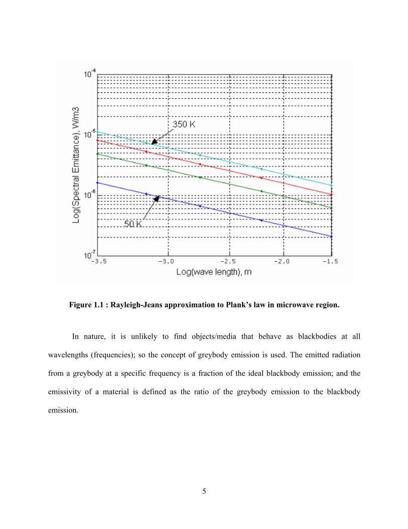
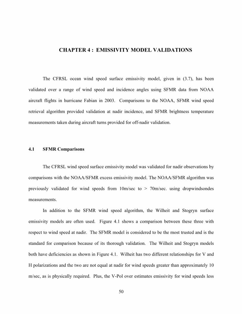
Figure 1.1 : Rayleigh-Jeans approximation to Plank’s law in microwave region.
In nature, it is unlikely to find objects/media that behave as blackbodies at all
wavelengths (frequencies); so the concept of greybody emission is used. The emitted radiation
from a greybody at a specific frequency is a fraction of the ideal blackbody emission; and the
emissivity of a material is defined as the ratio of the greybody emission to the blackbody
emission.
5
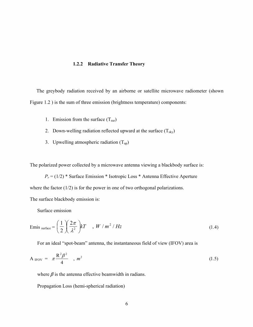
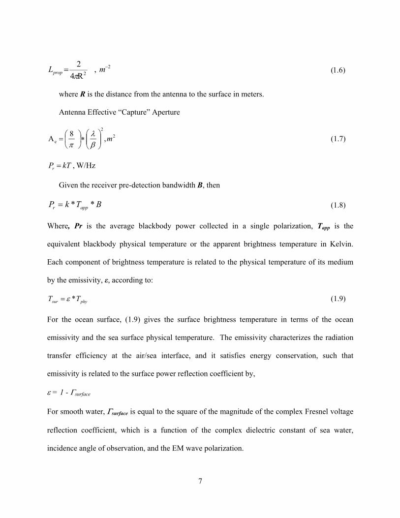
1.2.2 Radiative Transfer Theory
The greybody radiation received by an airborne or satellite microwave radiometer (shown
Figure 1.2 ) is the sum of three emission (brightness temperature) components:
1. Emission from the surface (Tsur)
2. Down-welling radiation reflected upward at the surface (Tsky)
3. Upwelling atmospheric radiation (Tup)
The polarized power collected by a microwave antenna viewing a blackbody surface is:
Pr = (1/2) * Surface Emission * Isotropic Loss * Antenna Effective Aperture
where the factor (1/2) is for the power in one of two orthogonal polarizations.
The surface blackbody emission is:
Surface emission
Emis surface = HzmWkT //, 221 2
2 ⎟⎠⎞
⎜⎝⎛
⎟⎠⎞
⎜⎝⎛
λπ
)4.1(
For an ideal “spot-beam” antenna, the instantaneous field of view (IFOV) area is
A IFOV = 222
,4
R mβπ )5.1(
where β is the antenna effective beamwidth in radians.
Propagation Loss (hemi-spherical radiation)
6
22 ,
R42 −= mLprop π
)6.1(
where R is the distance from the antenna to the surface in meters.
Antenna Effective “Capture” Aperture
22
e ,8 A m⎟⎟⎠
⎞⎜⎜⎝
⎛∗⎟
⎠⎞
⎜⎝⎛ =
βλ
π (1.7)
W/Hz, kTPr =
Given the receiver pre-detection bandwidth B, then
BTkP appr **= (1.8)
Where, Pr is the average blackbody power collected in a single polarization, Tapp is the
equivalent blackbody physical temperature or the apparent brightness temperature in Kelvin.
Each component of brightness temperature is related to the physical temperature of its medium
by the emissivity, ε, according to:
physur TT *ε= (1.9)
For the ocean surface, (1.9) gives the surface brightness temperature in terms of the ocean
emissivity and the sea surface physical temperature. The emissivity characterizes the radiation
transfer efficiency at the air/sea interface, and it satisfies energy conservation, such that
emissivity is related to the surface power reflection coefficient by,
ε = 1 - Γsurface
For smooth water, Γsurface is equal to the square of the magnitude of the complex Fresnel voltage
reflection coefficient, which is a function of the complex dielectric constant of sea water,
incidence angle of observation, and the EM wave polarization.
7
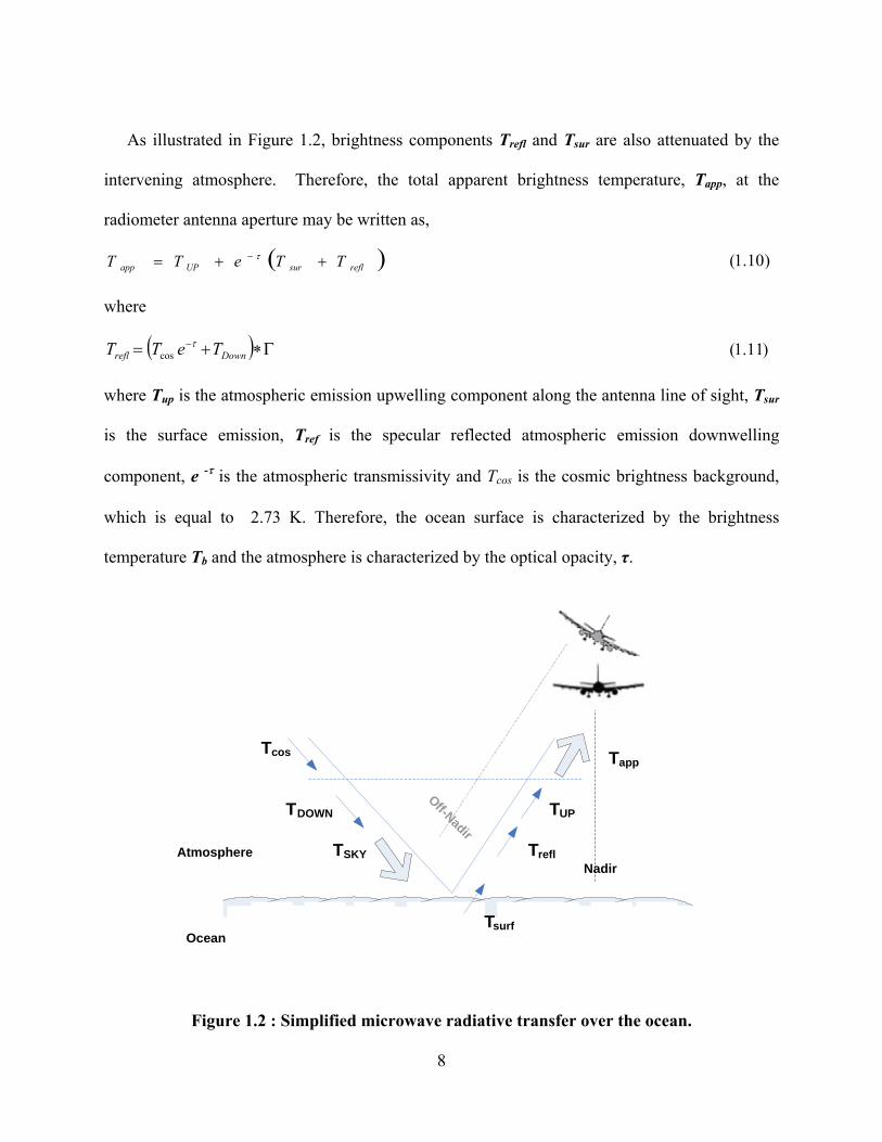
As illustrated in Figure 1.2, brightness components Trefl and Tsur are also attenuated by the
intervening atmosphere. Therefore, the total apparent brightness temperature, Tapp, at the
radiometer antenna aperture may be written as,
( )reflsurUPapp TTeTT ++= − τ )10.1(
where
( ) Γ∗+= −Downrefl TeTT τ
cos )11.1(
where Tup is the atmospheric emission upwelling component along the antenna line of sight, Tsur
is the surface emission, Tref is the specular reflected atmospheric emission downwelling
component, e -τ is the atmospheric transmissivity and Tcos is the cosmic brightness background,
which is equal to 2.73 K. Therefore, the ocean surface is characterized by the brightness
temperature Tb and the atmosphere is characterized by the optical opacity, τ.
Atmosphere
Ocean
Tcos
TDOWN
TSKY
TUP
Trefl
Tsurf
Tapp
Nadir
Off-Nadir
Figure 1.2 : Simplified microwave radiative transfer over the ocean.
8
1.3 Ocean Surface Wind Speed Remote Sensing
Surface winds cause roughening of the ocean surface by the generation of small ocean
waves of cm length. Roughening the surface decreases the power reflectivity and therefore
increases the emissivity. Further, with time, the small waves transfer their energy to longer
waves that eventually break and form white caps and foam patches. Foam has low reflectivity
and can be considered as approximately a blackbody. The monotonic growth of the percentage of
foam (foam fraction) coverage is the means to estimate the surface wind speed from measured
brightness temperatures. For high wind speeds, such as in hurricanes, foam emission is dominant
in the radiometer received signal. The objective of this thesis is to develop a physics-based wind
speed model useful from low wind speeds approaching zero m/sec to category-5 hurricane wind
speeds of > 70 m/sec.
1.3.1 Satellite Radiometers
Microwave radiometers that are widely used on weather satellites usually operate at
number of frequencies (wavelengths) to separate the various Tb contributions from the surface
and atmosphere. For example, weather satellites with multi-frequency radiometers are able to
retrieve geophysical parameters like water vapor, cloud liquid water, rain rate for the atmosphere
and ocean wind speed, and land/sea surface temperature for the earth surface. The use of
9
microwave frequencies has the advantage of penetrating clouds, haze, smoke, light rain and
snow; so microwave radiometers do not require clear skies to function properly.
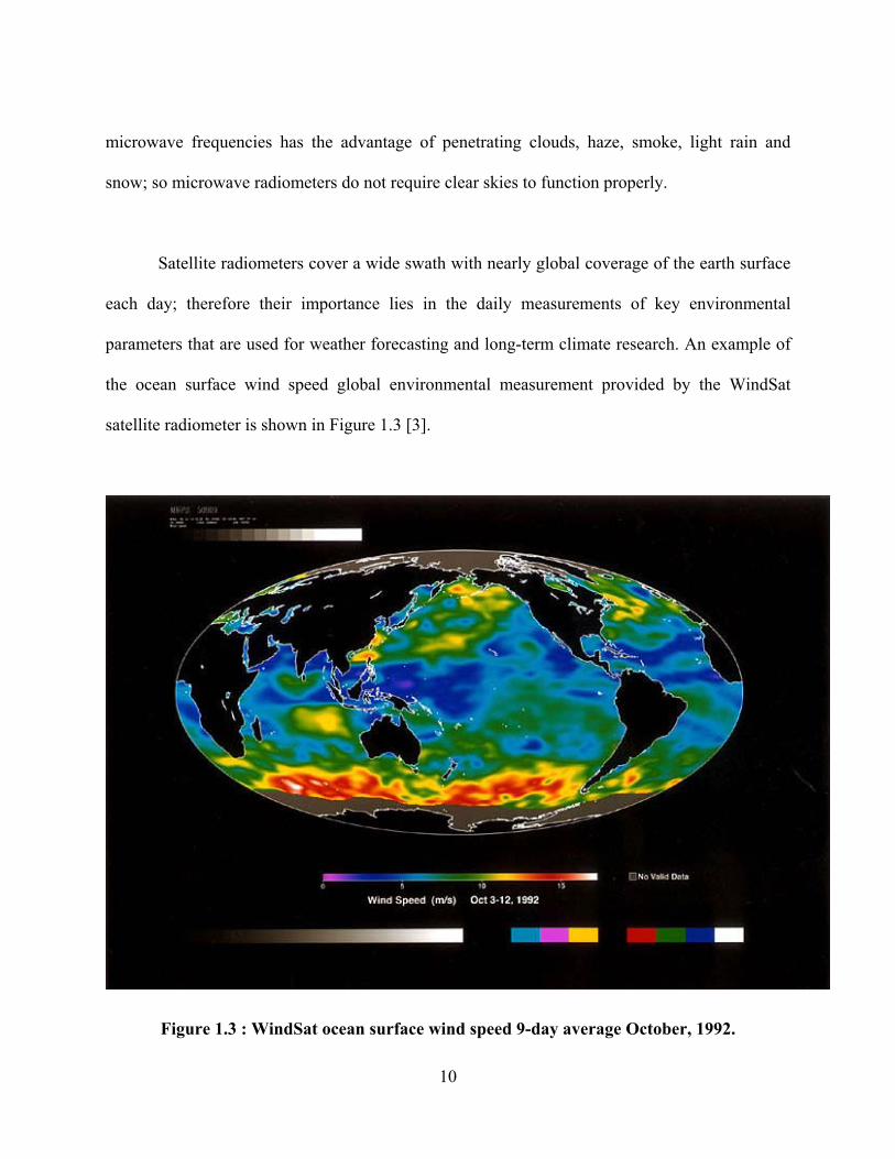
Satellite radiometers cover a wide swath with nearly global coverage of the earth surface
each day; therefore their importance lies in the daily measurements of key environmental
parameters that are used for weather forecasting and long-term climate research. An example of
the ocean surface wind speed global environmental measurement provided by the WindSat
satellite radiometer is shown in Figure 1.3 [3].
Figure 1.3 : WindSat ocean surface wind speed 9-day average October, 1992.
10
1.3.2 SFMR Measurements
The measurement of hurricane maximum (one-minute sustained) surface winds is a
requirement of the National Oceanic Atmospheric Administration’s (NOAA) Tropical Prediction
Center/National Hurricane Center (TPC/NHC). The NOAA/Hurricane Research Division's
(HRD) Stepped-Frequency Microwave Radiometer (SFMR) is the prototype for a new
generation of operational airborne remote sensing instruments designed for surface wind and rain
measurements in hurricanes. The first experimental SFMR surface wind measurements were
made in Hurricane Allen in 1980 [4], the first real-time retrieval of winds on board the aircraft in
Hurricane Earl in 1985, and the first operational real-time transmission of winds to TPC/NHC in
Hurricane Dennis in 1999 [5]. The use of the C-band frequency range from 4.5-7.22 GHz
provides the ability to penetrate clouds and heavy rain and thereby to measure wind speeds on
the surface and rain rate simultaneously.
The research performed in this thesis used Tb measurements collected by the SFMR at
nadir and during aircraft banks for modeling nadir and off-nadir ocean surface emissivity, as will
be described later in the coming chapters. Chapter 2 discusses the theoretical sea surface
emission for smooth water and several semi-empirical rough ocean emissivity models. Next,
Chapter 3 presents the development of the C-band wind speed emissivity model for nadir and off
nadir viewing; and Chapter 4 discusses the validation of this C-band emissivity model with
11
measurements from SFMR. Finally Chapter 5 presents conclusion and recommendations for
future work.
12
CHAPTER 2 : SEA SURFACE EMISSION
The principal component in the C-band microwave ocean RTM is the emission from the
surface. It represents the largest portion from the received brightness temperature that is about
95% of the total emission with no rain. The emissivity of the surface is proportional to sea
surface temperature, salinity, frequency and surface roughness and is modeled in to two parts:
1. Emission for a smooth specular surface
2. Emission for a rough surface
The contribution of each in the total surface emission will be described in the sections that
follow.
2.1 Physical Principles
In remote sensing, understanding the physics of EM wave propagation across a boundary
between two dielectric media is essential to the interpretation of radiometric signals. For a
microwave radiometer viewing a smooth ocean surface through a non-attenuating atmosphere,
the EM propagation across the air/sea interface depends upon the difference in the characteristic
impedances of the two media.
13
2.1.1 Fresnel Voltage Reflection Coefficient
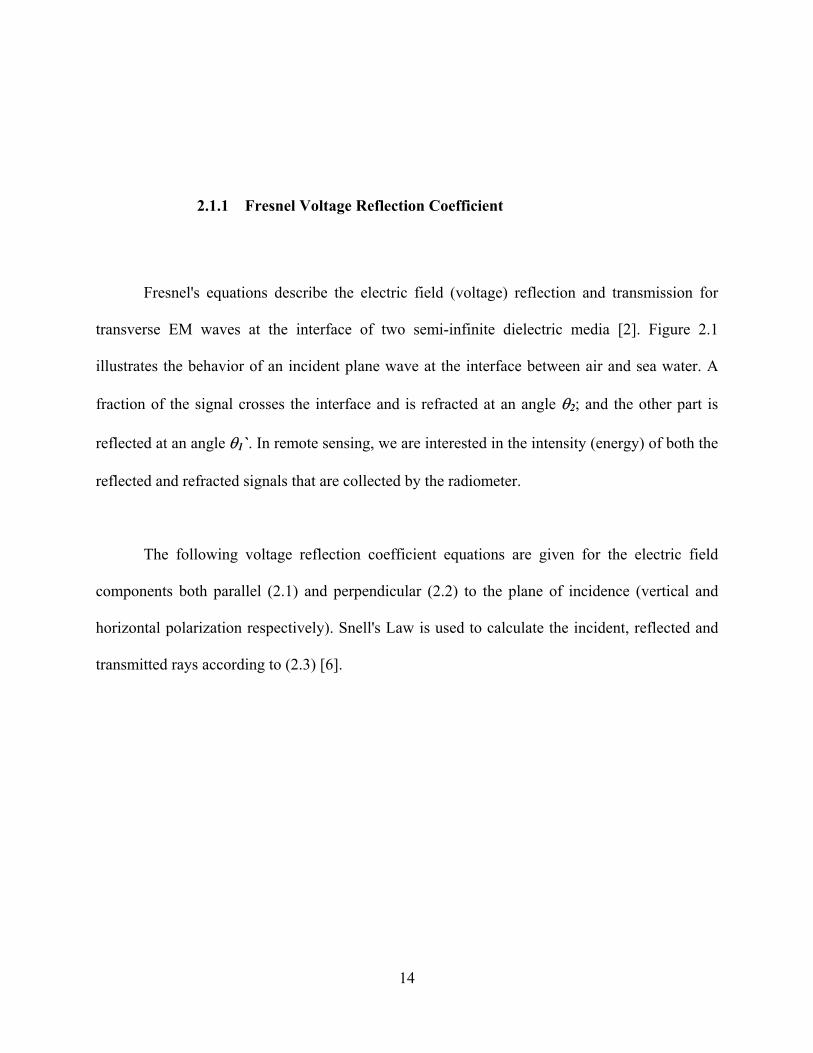
Fresnel's equations describe the electric field (voltage) reflection and transmission for
transverse EM waves at the interface of two semi-infinite dielectric media [2]. Figure 2.1
illustrates the behavior of an incident plane wave at the interface between air and sea water. A
fraction of the signal crosses the interface and is refracted at an angle θ2; and the other part is
reflected at an angle θ1`. In remote sensing, we are interested in the intensity (energy) of both the
reflected and refracted signals that are collected by the radiometer.
The following voltage reflection coefficient equations are given for the electric field
components both parallel (2.1) and perpendicular (2.2) to the plane of incidence (vertical and
horizontal polarization respectively). Snell's Law is used to calculate the incident, reflected and
transmitted rays according to (2.3) [6].
14
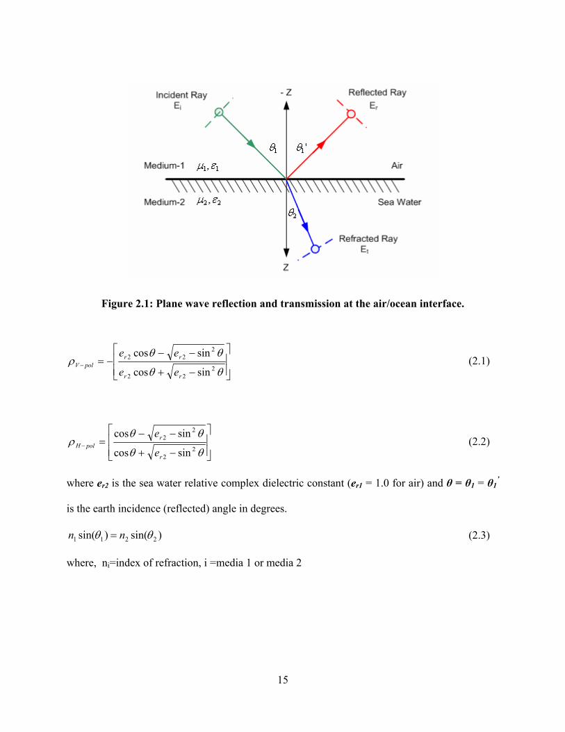
Figure 2.1: Plane wave reflection and transmission at the air/ocean interface.
⎥⎥⎦
⎤
⎢⎢⎣
⎡
−+
−−−=−
θθ
θθρ
222
222
sincos
sincos
rr
rrpolV
ee
ee (2.1)
⎥⎥⎦
⎤
⎢⎢⎣
⎡
−+
−−=−
θθ
θθρ
22
22
sincos
sincos
r
rpolH
e
e (2.2)
where er2 is the sea water relative complex dielectric constant (er1 = 1.0 for air) and θ = θ1 = θ1’
is the earth incidence (reflected) angle in degrees.
)sin()sin( 2211 θθ nn = (2.3)
where, ni=index of refraction, i =media 1 or media 2
15
Figure 2.2 : Typical ocean power reflection coefficient.
In Figure 2.2, the H-pol power reflection coefficient increases monotonically to unity
reflection at an incidence angle of 90 deg, and the V-pol curve decreases and reaches zero
reflection at an angle ~ 83 deg, known as the Brewster angle. At this incidence angle, there is no
reflection and the wave passes through the interface without refraction. At larger incidence
angles, the reflection rapidly increases to 100% at 90 deg.
16
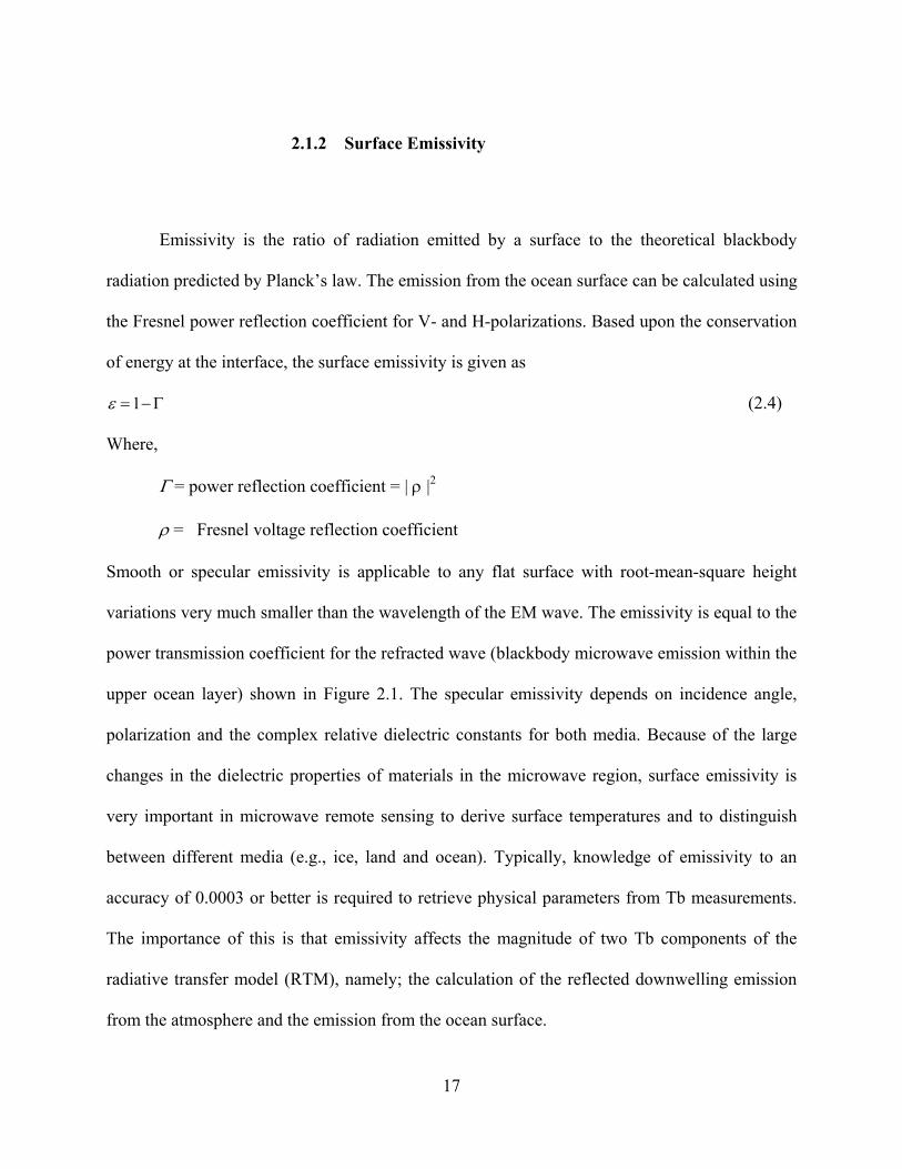
2.1.2 Surface Emissivity
Emissivity is the ratio of radiation emitted by a surface to the theoretical blackbody
radiation predicted by Planck’s law. The emission from the ocean surface can be calculated using
the Fresnel power reflection coefficient for V- and H-polarizations. Based upon the conservation
of energy at the interface, the surface emissivity is given as
Γ−=1ε (2.4)
Where,
Γ = power reflection coefficient = | ρ |2
ρ = Fresnel voltage reflection coefficient
Smooth or specular emissivity is applicable to any flat surface with root-mean-square height
variations very much smaller than the wavelength of the EM wave. The emissivity is equal to the
power transmission coefficient for the refracted wave (blackbody microwave emission within the
upper ocean layer) shown in Figure 2.1. The specular emissivity depends on incidence angle,
polarization and the complex relative dielectric constants for both media. Because of the large
changes in the dielectric properties of materials in the microwave region, surface emissivity is
very important in microwave remote sensing to derive surface temperatures and to distinguish
between different media (e.g., ice, land and ocean). Typically, knowledge of emissivity to an
accuracy of 0.0003 or better is required to retrieve physical parameters from Tb measurements.
The importance of this is that emissivity affects the magnitude of two Tb components of the
radiative transfer model (RTM), namely; the calculation of the reflected downwelling emission
from the atmosphere and the emission from the ocean surface.
17
2.1.3 Dielectric Constant of Sea Water
Precise knowledge of the complex dielectric constant (permittivity) εr of water is
essential for studying the radiative transfer of microwave radiation that is emitted by the ocean
surface. The dielectric constant is a function of frequency (f), surface water temperature T and
salinity S, as shown in the Debye equation [6].
⎟⎠⎞
⎜⎝⎛−
⎟⎠⎞
⎜⎝⎛+
−+= −
∞∞ c
jj R
sr
σλ
λλ
εεεε η
2
11 (2.5)
Where,
1−=j
λ = radiation wavelength in cm
ε∞ = dielectric constant at infinite frequency
εS = static dielectric constant at zero frequency
λR = relaxation wavelength in cm.
η = spread factor
σ = is the ionic conductivity determined by the dissolved salt content in S-1
c = is the speed of light in cm/sec
Over the past four decades several Debye models have been developed using experimental
microwave measurements of pure and saline water [7, 8], but the latest and the one that is used in
this thesis was developed by Meissner and Wentz [9] to match satellite radiometer measurements
18
over a wide range of frequencies. Figure 2.3 shows the real and imaginary parts of the dielectric
constant versus frequency for fresh (salinity = 0 ppt) and salt water (salinity = 33 ppt) and a sea
surface temperature of 20 °C.
19
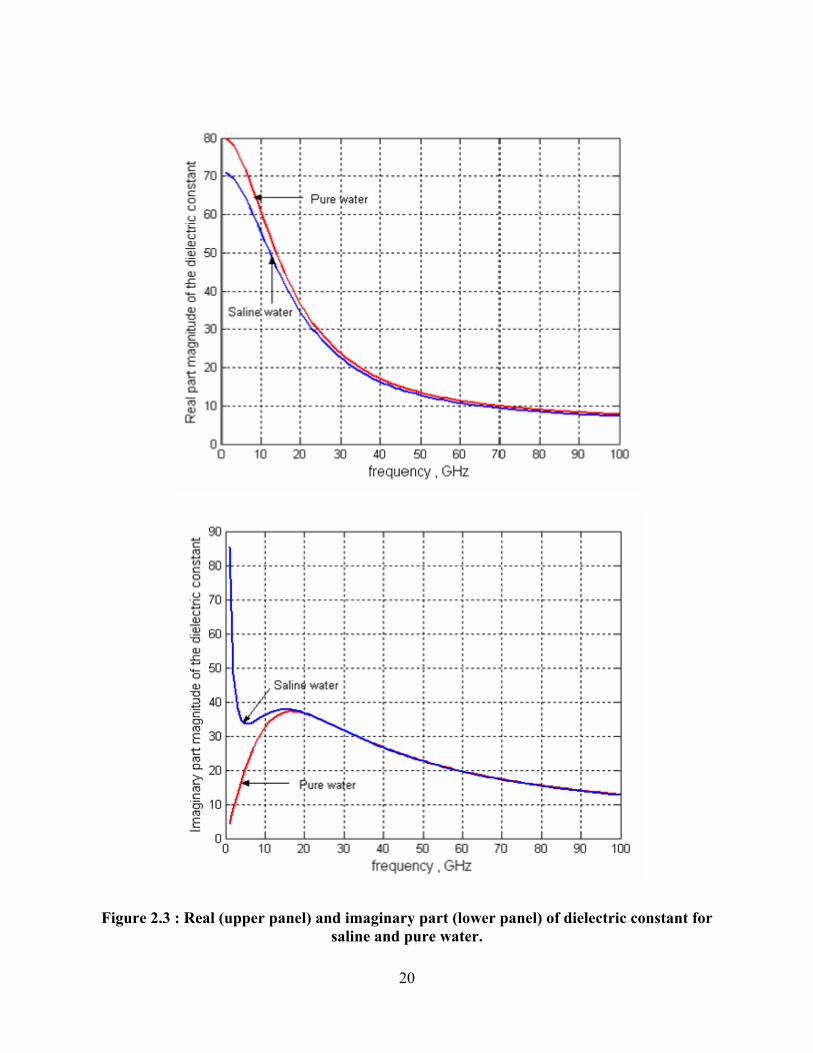
Figure 2.3 : Real (upper panel) and imaginary part (lower panel) of dielectric constant for saline and pure water.
20
2.2 Sea Surface Emissivity
Traditionally, the sea surface emissivity has been modeled as the sum of a specular
emissivity (based upon Fresnel reflection coefficient) plus a wind speed dependant rough
emissivity that has been empirically determined such as in Stogryn [10], as shown in (2.6).
roughsmoothtotal εεε += (2.6)
2.2.1 Smooth Water Emissivity
Applying the principal of the conservation of energy at the air/sea interface yields the
following definition for the smooth (specular) emissivity in (2.4). Because the smooth water
emissivity depends on Fresnel power reflection coefficient, it is a function of the complex
dielectric constant of sea water. Further, it should be noted that the dielectric constant is also a
function of the radiometer frequency, the water temperature and the salinity. A typical example
is given in Figure 2.4, where the emissivity response is reversed compared to the power
reflection coefficient i.e., V-pol increases and H-pol decreases versus incidence angle.
21
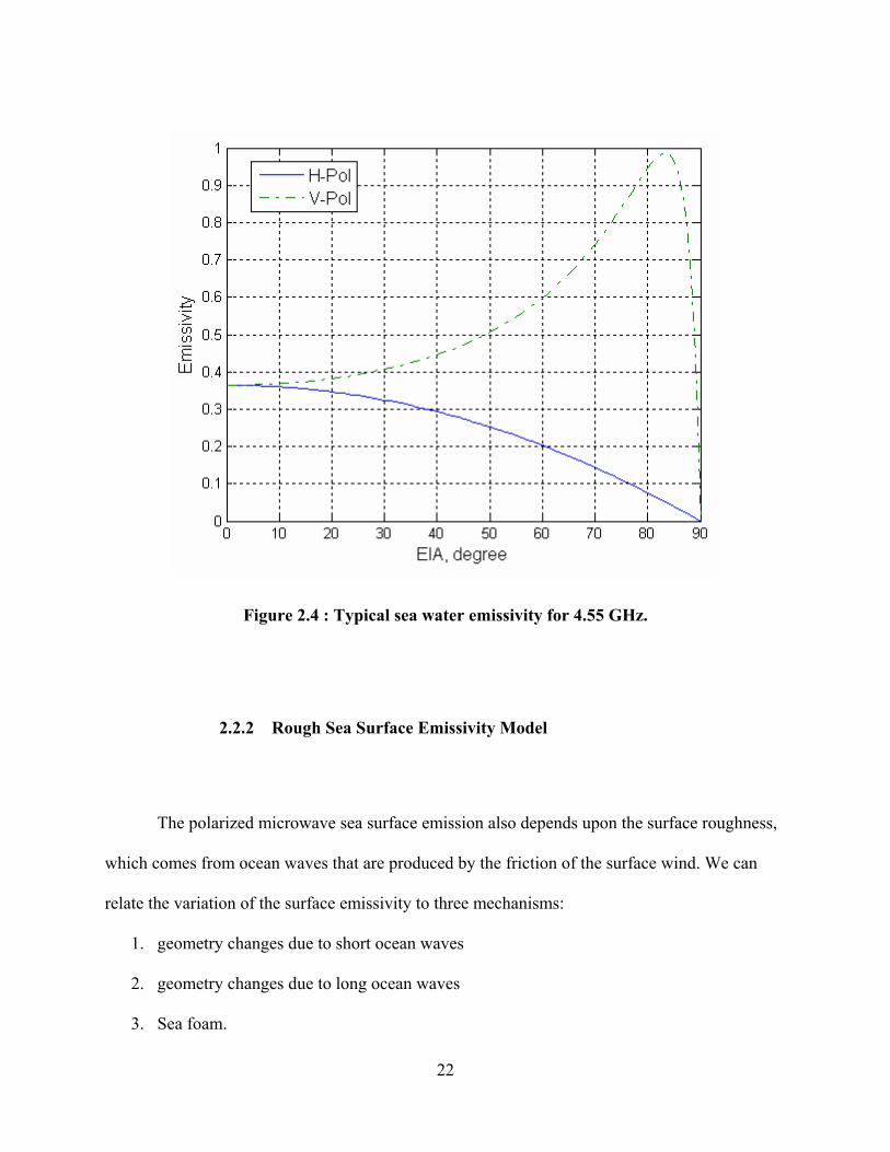
Figure 2.4 : Typical sea water emissivity for 4.55 GHz.
2.2.2 Rough Sea Surface Emissivity Model
The polarized microwave sea surface emission also depends upon the surface roughness,
which comes from ocean waves that are produced by the friction of the surface wind. We can
relate the variation of the surface emissivity to three mechanisms:
1. geometry changes due to short ocean waves
2. geometry changes due to long ocean waves
3. Sea foam.
22
The first has to do with diffraction of microwaves by short ocean waves that are small
comparable to the radiation wavelength. The second mechanism has to do with long ocean waves
compared to the radiation wavelength, which tilt the surface and thereby mix the H- and V-
polarizations and change the incidence angle of the incident wave. Both mechanisms can be
treated using a two-scale EM model of ocean facets that have their own reflection coefficient
[10]. The third mechanism deals with the generation of sea foam caused by breaking gravity
ocean waves. This has a large effect at high wind speeds due to the high emission of foam for
both polarizations. All the three mechanisms can be parameterized in terms of the surface wind
speed and relative wind direction (defined as azimuth viewing direction of the radiometer
relative to the wind direction).
Optical experiments conducted by Cox and Munk [11] measured the slope spectrum of
the ocean surface caused by surface winds. They based their findings on sun light that was
reflected from the rough ocean surface. Microwave radiometer researchers such as Stogryn [10],
have used the ocean slope spectrum results of Cox and Munk to model the microwave ocean
emission as a function of surface wind speed microwave frequency and polarization, and these
models have been verified over a range of wind speeds and EIA’s, in numerous field
measurements using ocean plateforms, aircraft, and satellite measurements [12, 13]. An example
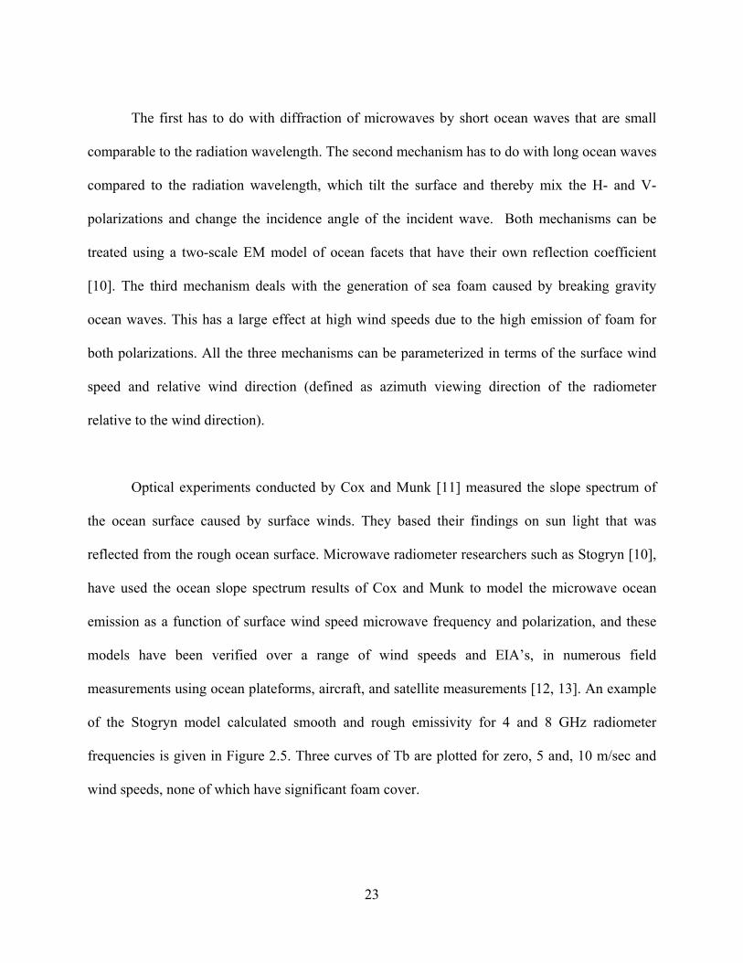
of the Stogryn model calculated smooth and rough emissivity for 4 and 8 GHz radiometer
frequencies is given in Figure 2.5. Three curves of Tb are plotted for zero, 5 and, 10 m/sec and
wind speeds, none of which have significant foam cover.
23
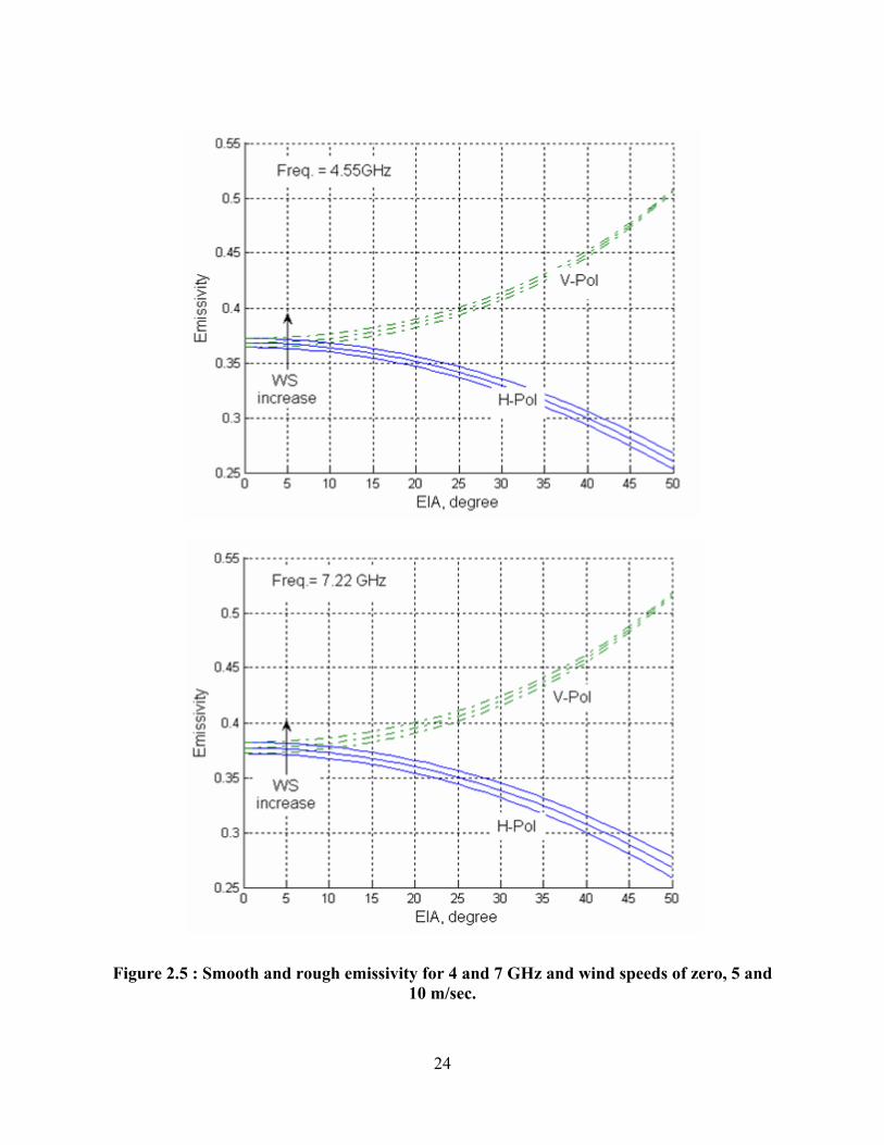
Figure 2.5 : Smooth and rough emissivity for 4 and 7 GHz and wind speeds of zero, 5 and 10 m/sec.
24
2.3 Sea Foam
Most microwave RTM’s treat sea foam as an approximate blackbody with low
reflectivity and near-unity emissivity. The transformation of ocean wave energy from short to
long wavelengths causes the long gravity ocean wave heights and slopes to grow until gravity
causes them to break and produce “white caps” and foam. Since the emissivity of foam is
approximately twice that of sea water, understanding the EM characteristics of foam and how it
is produced and distributed over the ocean surface is crucial to calculating the rough surface
emissivity.
2.3.1 Effect of Foam on Oceanic Emission
Modeling the ocean surface emissivity depends on both smooth and rough surface
emission modeling including the emission from foam, which becomes the dominant factor at
higher wind speeds. Foam is produced by breaking waves on ocean surface and is responsible for
increasing the emission from the foam-covered surface. The generally accepted hypothesis is
that, Sea foam is a medium comprising many small air bubbles that float on the ocean surface
and produce an impedance matching layer for the propagating EM waves (blackbody radiation in
the sea water medium). This reduces the internal blackbody radiation reflection at the air/sea
interface, which increases the ocean surface emissivity.
25
Many studies and experiments have been conducted to measure foam emission; as a
function of microwave frequency, polarization and incidence angle [14, 15]. Based upon these
experimental results, there are three major assumptions in modeling foam for an airborne
(spaceborne) radiometer. The first assumption is that there is a statistical randomness in area-
coverage distribution over the antenna foot print (instantaneous filed of view, IFOV) but that
each radiometer measurement contains the same mean area coverage of foam. The second is that
the foam layer is electromagnetically thick, which implies a thickness greater than a free space
wavelength. Third, and most important, is that there exists a statistically stationary relationship
between foam area coverage and surface wind speed. Also, in modeling foam emissivity we
assume that the foam emissivity is not a function of wind speed.
2.3.2 Emissivity of Foam
In 1970, an interesting attempt at a theoretical description of the emissivity of foam was
made by Droppleman [14], his conclusion was that the complexity of the EM boundary value
problem precluded the construction of a physically and mathematically convincing theoretical
model. Thus, at least for the present, complete reliance must be placed on experimental data in
studies relating to the radiometric effects of foam and its relationship with frequency and
incidence angle.
26
In 1972, Stogryn [15] developed an empirical expression for sea foam emissivity as a
function of sea surface temperature, frequency, and incidence angle based on a review of
previously published measurements of foam-covered sea surface. Recently, Rose et. al [16]
performed experiments at frequencies 10 and 37 GHz for the range of incidence angle from 30°
to 60°. Further, Padmanabhan et al. [17] performed foam emissivity experiments at three
frequencies (10, 19 and 37 GHz ) for 53° incidence. The emissivity of foam is approximately two
times higher than that of calm water, which emphasizes the necessity to account for foam in the
calculations of the total emissivity.
2.3.3 Foam Fraction - Wind Speed Dependence
Based upon empirical results, the formation of foam is highly correlated with surface
wind speed and the breaking of gravity ocean waves. Foam fraction or area percentage of foam
coverage increases with wind speed and is randomly distributed over the ocean surface on a
spatial scale of 10’s of meters. Because airborne radiometer antennas have footprints on the
ocean surface of 100’s meters diameters, the location of foam will appear uniformly distributed
in an average sense. A recent study, to characterize the increase of foam fraction, used aerial
photography taken at low-altitudes in hurricanes to study the white caps coverage (WCC) and
foam coverage with wind speed [18].
27
Foam fraction is, obviously, independent of the radiometer parameters; frequency,
polarization and incidence angle; therefore, it is modeled as a function of wind speed only.
Foam begins to appear on the ocean surface at wind speeds of approximately
6 m/sec, where breaking waves start to form, and it increases approximately exponentially with
wind speed. For example, from this thesis analysis at a wind speed of 70 m/sec, the foam
coverage is estimated to be ~ 80 %. At higher wind speeds, we assume that the percentage foam
cover asymptotically approaches 100 %.
28
CHAPTER 3 : WIND SPEED EMISSIVITY MODEL DEVELOPMENT
Experimentally, it has been observed that the surface wind over the ocean exhibits a
strong modulation of the brightness temperature (surface emissivity). The importance of
modeling the surface emissivity is that it affects the direct emission from the sea surface as well
as the reflected downwelling brightness temperature from the atmosphere. Unfortunately,
theoretical radiometric modeling of this rough surface emissivity has been challenging and of
only limited success. One reason for this is that the small-scale ocean wave characteristics and
their dependence on frictional wind drag on the ocean’s surface are not well understood - mostly
due to the difficulty of making the required wave measurements in the ocean environment. As a
result, radiometric modelers have developed empirical relationships between the surface wind
speed and the observed excess brightness temperature. In this chapter, selected models will be
described as they relate to this thesis development of a high wind speed emissivity model for use
in hurricane research.
3.1 Existing Wind Speed Emissivity Models
For smooth ocean surfaces, Fresnel power reflection coefficients are used to model the
emissivity with respect to frequency, polarization and incidence angle as given in equation (2.1),
(2.2) and (2.3). For slightly rough surfaces (wind speeds < 7 m/sec), there are both quasi-
theoretical and strictly empirical approaches that are reasonably successful. Beyond 7 m/sec the
breaking of ocean waves creates foam, which exhibits high emissivity. The foam percentage area
29
coverage varies with the surface wind speed, and this must be known to model the ocean
emissivity. Empirical foam and ocean roughness radiometric models exist to characterize the
emissivity up to approximately 20 m/sec. Beyond 20 m/sec, the ocean emissivity is not well
known because of the rarity of radiometric observations of such events.
3.1.1 Near-Nadir Models
For low wind speeds, the wind friction produced at the air/sea interface generates short
ocean (capillary) waves, which increases the emissivity over that calculated using Fresnel power
reflection coefficient.
One example of an emissivity model is Wilheit surface emissivity model, which is a
function of EIA as well [12]. Wilheit combines the effect due to rough surfaces and foam
formation in one term and then calculate his surface emissivity as shown in (3.1), and he divided
his wind speed dependence function to three different wind speed regions: ws ≤ than 7m/sec,
7 < ws < 17 m/sec and ws ≥ 17 m/sec. In these three regions, he models the wind speed as linear,
quadratic and then linear dependence for each region, respectively.
( ) roughnnTotal EFFEmissivity −+= 1 (3.1)
Where,
Fn = is a function of wind speed, n =1, 2, 3 wind speed regions
Erough = the rough water emissivity.
30
Another thing to note about this model is that it uses the Lane and Saxton complex
dielectric constant for saline and pure water [19]. This model has been validated using satellite
measurements and ocean buoy wind speed measurements [12].
Another well popular surface emissivity model was developed by Stogryn [10] which is a
function of EIA as well, This model treated total emissivity as the sum of two parts as shown in
(3.2).
Emissivity total = α * foam emissivity + (1- α)*foam free emissivity (3.2)
Where,
α = percentage of foam coverage.
Stogryn based his model on measurements collected from research papers and laboratory
experiments of foam coverage due to high winds which saturate foam at 35 m/sec to be 100%
covering the ocean surface. In (3.2), it can be noticed that the foam has a big contribution on the
total emissivity as wind speed increases.
The NOAA/SFMR wind speed algorithm is an empirical algorithm which regresses
SFMR brightness temperature at the ocean surface against independent measurements of surface
wind speed. It is applicable for nadir retrievals only and has been validated over a wide range of
wind speed from 10 m/sec to > 70m/sec [5]. This yields the excess emissivity, which is the delta
emissivity above a specular surface, as a function of frequency and wind speed given as:
31
( )( ) .sec/2.331 1012
2. mWSFreqbaWSaWSaExcess Emis <+++= (3.3)
( )( ) .sec/2.331 101. mWSFreqbcWScExcess Emis >++= (3.4)
Where,
WS = wind speed in m/sec.
Freq. = frequency in GHz.
an = wind speed coefficients, where n = 0,1,2
b1= frequency coefficient.
cn = wind speed coefficients, where n = 0,1
NOAA SFMR algorithm was modified after the 2005 hurricane season after observing
hurricanes with higher wind speeds than previously (> 70 m/sec), like Kartina 2005.
Figure 3.1, shows the SFMR excess emissivity curves for six frequencies versus wind
speed. The excess emissivity increases monotonically with wind speed and also, the emissivity
increases weakly with frequency as seen by the spread of curves at high wind speed.
32
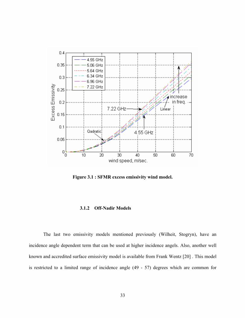
Figure 3.1 : SFMR excess emissivity wind model.
3.1.2 Off-Nadir Models
The last two emissivity models mentioned previously (Wilheit, Stogryn), have an
incidence angle dependent term that can be used at higher incidence angels. Also, another well
known and accredited surface emissivity model is available from Frank Wentz [20] . This model
is restricted to a limited range of incidence angle (49 - 57) degrees which are common for
33
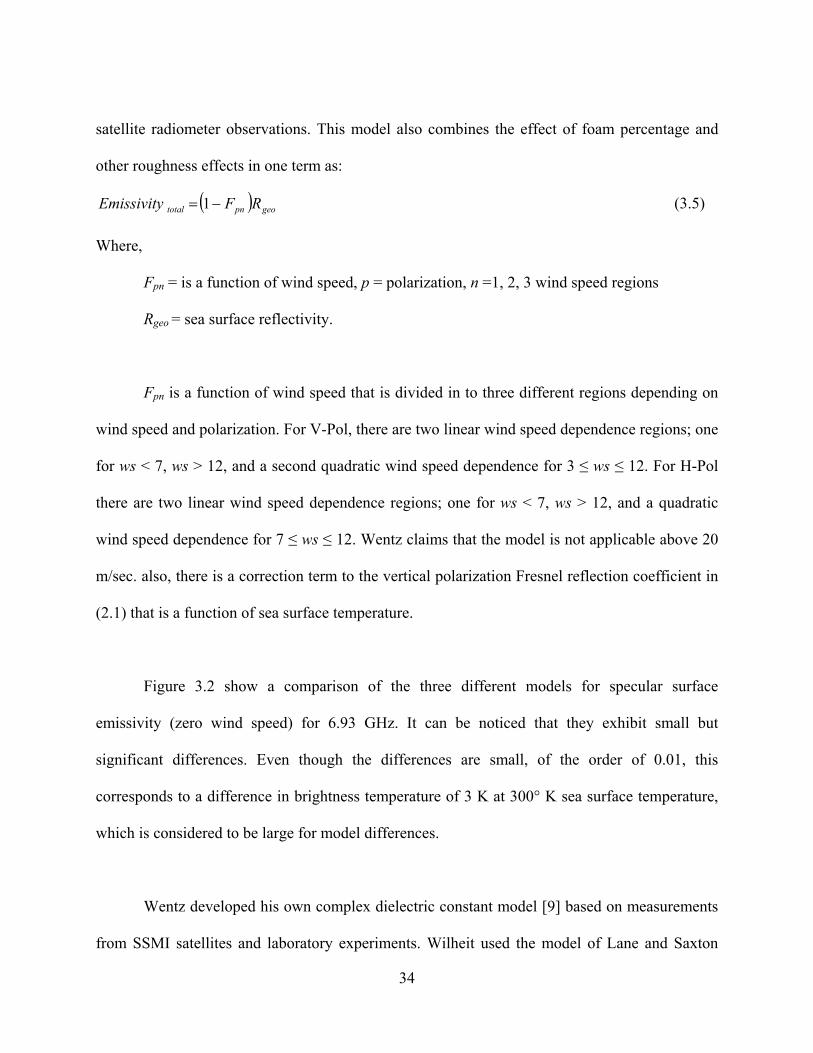
satellite radiometer observations. This model also combines the effect of foam percentage and
other roughness effects in one term as:
( ) geopntotal RFEmissivity −= 1 (3.5)
Where,
Fpn = is a function of wind speed, p = polarization, n =1, 2, 3 wind speed regions
Rgeo = sea surface reflectivity.
Fpn is a function of wind speed that is divided in to three different regions depending on
wind speed and polarization. For V-Pol, there are two linear wind speed dependence regions; one
for ws < 7, ws > 12, and a second quadratic wind speed dependence for 3 ≤ ws ≤ 12. For H-Pol
there are two linear wind speed dependence regions; one for ws < 7, ws > 12, and a quadratic
wind speed dependence for 7 ≤ ws ≤ 12. Wentz claims that the model is not applicable above 20
m/sec. also, there is a correction term to the vertical polarization Fresnel reflection coefficient in
(2.1) that is a function of sea surface temperature.
Figure 3.2 show a comparison of the three different models for specular surface
emissivity (zero wind speed) for 6.93 GHz. It can be noticed that they exhibit small but
significant differences. Even though the differences are small, of the order of 0.01, this
corresponds to a difference in brightness temperature of 3 K at 300° K sea surface temperature,
which is considered to be large for model differences.
Wentz developed his own complex dielectric constant model [9] based on measurements
from SSMI satellites and laboratory experiments. Wilheit used the model of Lane and Saxton
34
[19] which has been improved by Stogryn [8] and Klien and Swift [7]. Stogryn based his
complex dielectric constant model in part using studies taken by Lane and Saxton [20].
Figure 3.2 : Stogryn, Wilheit and Wentz wind speed model comparison for a wind speed of zero m/sec and Freq. = 6.93GHz.
Figure 3.3 shows a comparison for the rough emissivity models of the three modelers
(Wilheit, Stogryn and Wentz) for 6.93 GHz. Again there are significant differences between
models
35
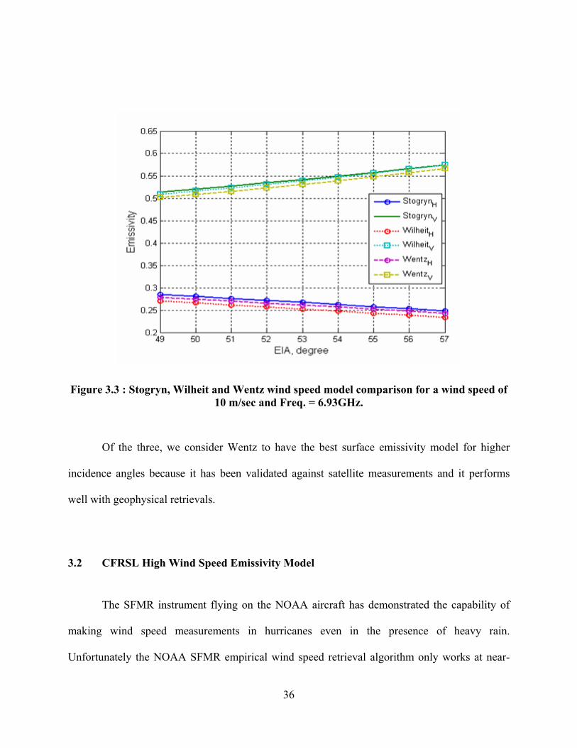
Figure 3.3 : Stogryn, Wilheit and Wentz wind speed model comparison for a wind speed of 10 m/sec and Freq. = 6.93GHz.
Of the three, we consider Wentz to have the best surface emissivity model for higher
incidence angles because it has been validated against satellite measurements and it performs
well with geophysical retrievals.
3.2 CFRSL High Wind Speed Emissivity Model
The SFMR instrument flying on the NOAA aircraft has demonstrated the capability of
making wind speed measurements in hurricanes even in the presence of heavy rain.
Unfortunately the NOAA SFMR empirical wind speed retrieval algorithm only works at near-
36
nadir and cannot be easily extended to off-nadir (high EIA) measurements that are required for
future airborne radiometer instruments. Thus, the CFRSL high wind speed emissivity model
(this thesis) was developed to remove these shortcomings and provide the basis for an improved
microwave radiative transfer model for hurricanes. The derivation of this CFRSL model is
discussed in this section. The main objective is to provide an emissivity model with the wind
speed response that matches that of the SFMR at nadir but also with off-nadir incidence angle
capability.
3.2.1 Near Nadir High Wind Speed Modeling
Modeling the surface in the presence of high wind speeds is difficult. The formation of
high emissivity foam and its direct relationship to wind speed complicates the model. Some
researchers combine the effect of foam and other roughness effects, like the Wilheit and Wentz
models discussed above; but others preferred to separate it, like Stogryn.
The CFRSL emissivity model presented below follows Stogryn and accounts for the
effects of foam on a physical basis. We choose to model the individual terms as follows:
ε = Tsur / SST (3.6)
where, SST is sea surface temperature (Kelvin). It follows that,
roughfreqfoam FFEIAfFF εεε *)1()(** _ −+= (3.7)
where, ε is total ocean surface emissivity
εfoam_freq is the frequency dependent emissivity of foam
37
f (EIA) is the earth incidence angle (EIA) dependence of foam
εrough is the rough sea surface emissivity
In (3.7) the only known quantity is the εrough and the assumption of f(EIA) to be equal to one at
nadir. The other parameters are derived from the NOAA SFMR algorithm and actual SFMR Tb
measurements in hurricanes. We justify using the NOAA SFMR excess emissivity [5] as “truth”
because this algorithm has demonstrated excellent wind speed retrieval accuracy as compared
with independent wind measurements over the range of 10 m/sec to > 70 m/sec. It must follow
that the correct characterization of emissivity versus wind speed is a necessary condition to
achieve accurate wind speed retrievals.
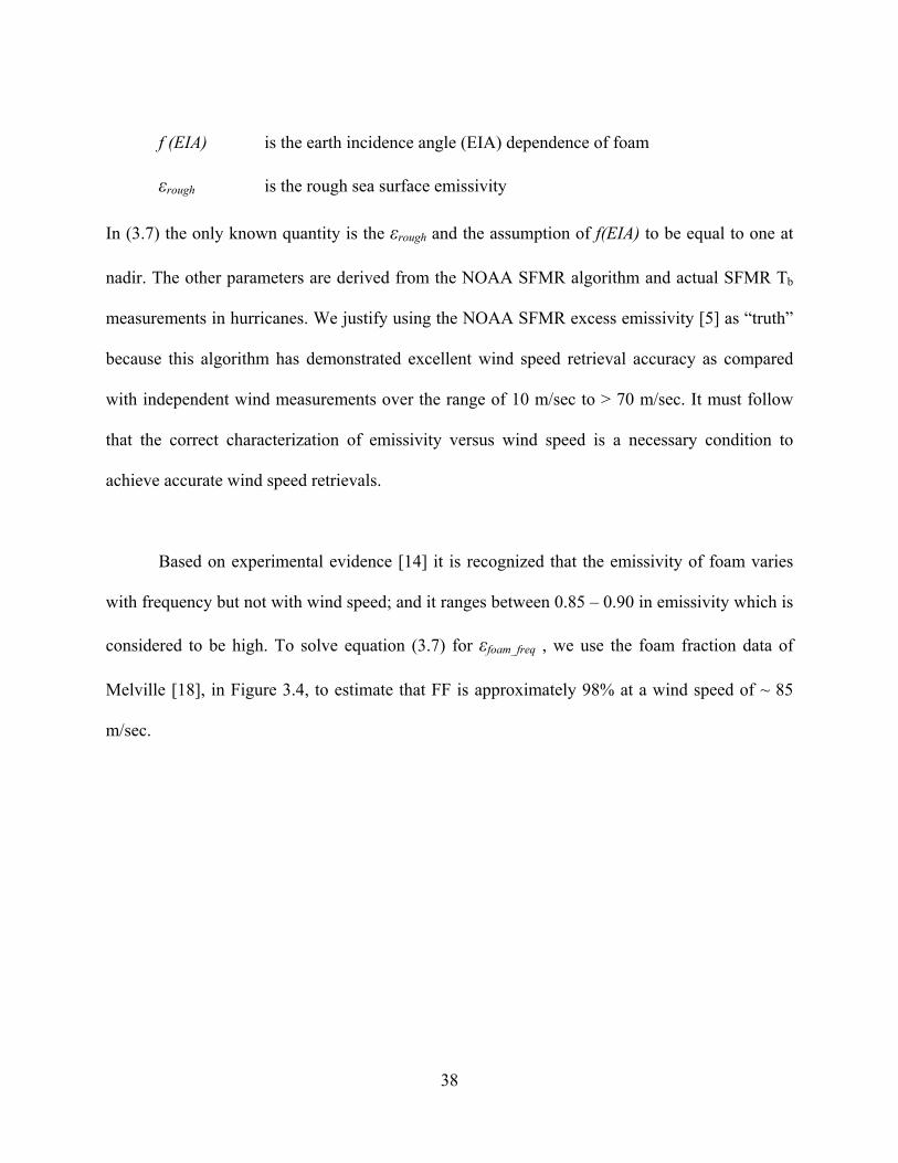
Based on experimental evidence [14] it is recognized that the emissivity of foam varies
with frequency but not with wind speed; and it ranges between 0.85 – 0.90 in emissivity which is
considered to be high. To solve equation (3.7) for εfoam_freq , we use the foam fraction data of
Melville [18], in Figure 3.4, to estimate that FF is approximately 98% at a wind speed of ~ 85
m/sec.
38
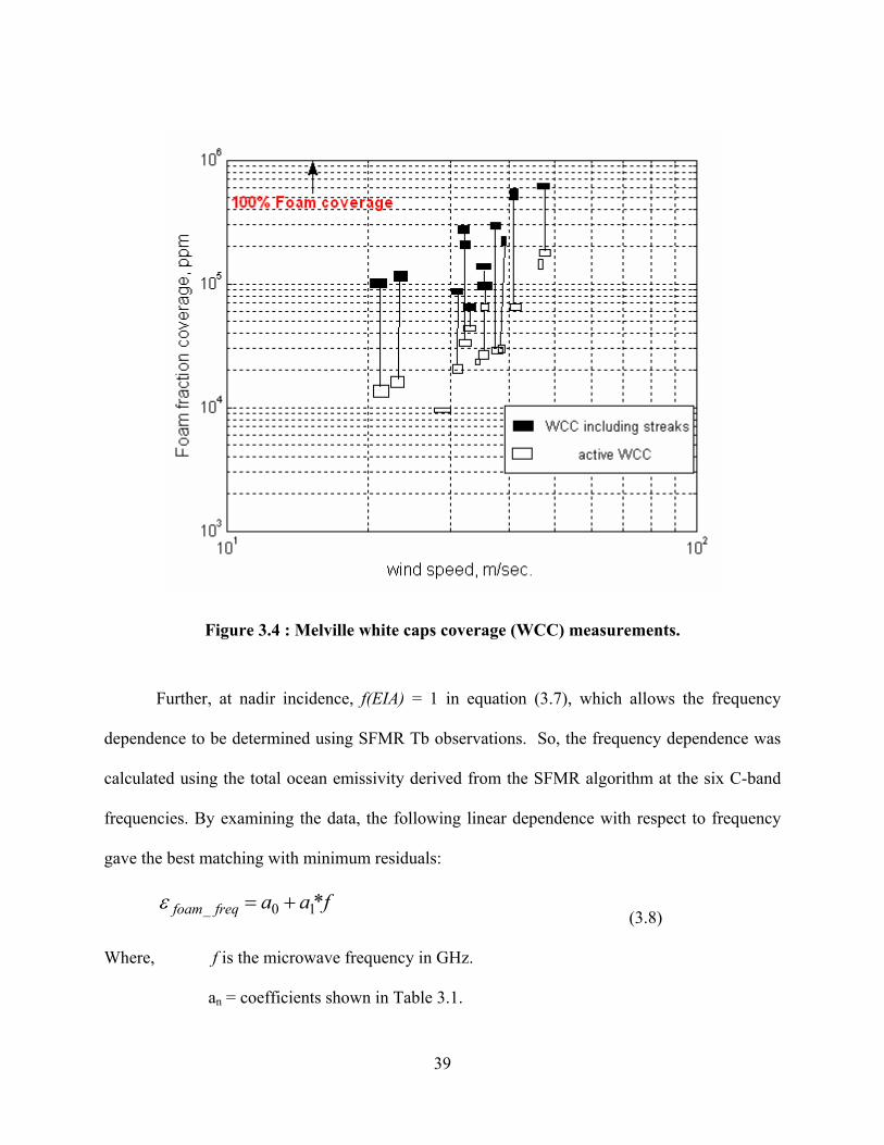
Figure 3.4 : Melville white caps coverage (WCC) measurements.
Further, at nadir incidence, f(EIA) = 1 in equation (3.7), which allows the frequency
dependence to be determined using SFMR Tb observations. So, the frequency dependence was
calculated using the total ocean emissivity derived from the SFMR algorithm at the six C-band
frequencies. By examining the data, the following linear dependence with respect to frequency
gave the best matching with minimum residuals:
*faafreqfoam 10_ +=ε
(3.8)
Where, f is the microwave frequency in GHz.
an = coefficients shown in Table 3.1.
39
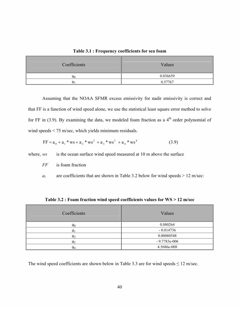
Table 3.1 : Frequency coefficients for sea foam
Coefficients
Values
a0 0.036659 a1 0.57767
Assuming that the NOAA SFMR excess emissivity for nadir emissivity is correct and
that FF is a function of wind speed alone, we use the statistical least square error method to solve
for FF in (3.9). By examining the data, we modeled foam fraction as a 4th order polynomial of
wind speeds < 75 m/sec, which yields minimum residuals.
(3.9) 44
33
2210 ws*a ws*a ws*a ws*a a FF ++++=
where, ws is the ocean surface wind speed measured at 10 m above the surface
FF is foam fraction
ai are coefficients that are shown in Table 3.2 below for wind speeds > 12 m/sec:
Table 3.2 : Foam fraction wind speed coefficients values for WS > 12 m/sec
Coefficients
Values
a0 0.080264 a1 - 0.014736 a2 0.00080548 a3 - 9.7783e-006 a4 4.5686e-008
The wind speed coefficients are shown below in Table 3.3 are for wind speeds ≤ 12 m/sec.
40
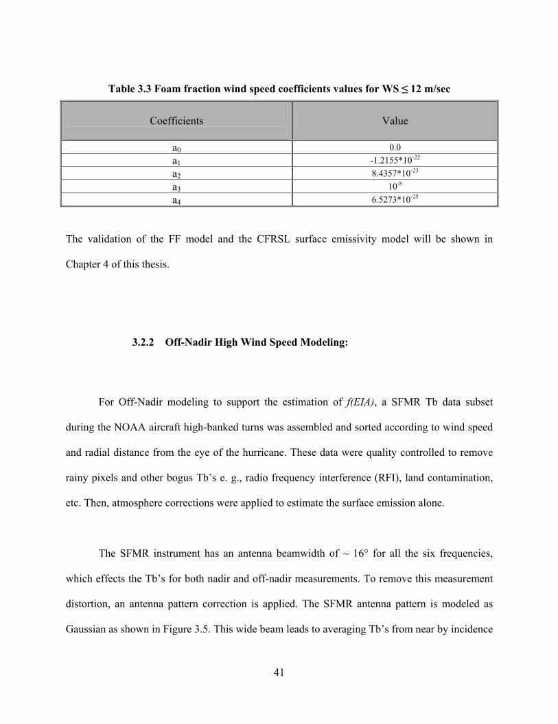
Table 3.3 Foam fraction wind speed coefficients values for WS ≤ 12 m/sec
Coefficients
Value
a0 0.0 a1 -1.2155*10-22 a2 8.4357*10-23 a3 10-8 a4 6.5273*10-25
The validation of the FF model and the CFRSL surface emissivity model will be shown in
Chapter 4 of this thesis.
3.2.2 Off-Nadir High Wind Speed Modeling:
For Off-Nadir modeling to support the estimation of f(EIA), a SFMR Tb data subset
during the NOAA aircraft high-banked turns was assembled and sorted according to wind speed
and radial distance from the eye of the hurricane. These data were quality controlled to remove
rainy pixels and other bogus Tb’s e. g., radio frequency interference (RFI), land contamination,
etc. Then, atmosphere corrections were applied to estimate the surface emission alone.
The SFMR instrument has an antenna beamwidth of ~ 16° for all the six frequencies,
which effects the Tb’s for both nadir and off-nadir measurements. To remove this measurement
distortion, an antenna pattern correction is applied. The SFMR antenna pattern is modeled as
Gaussian as shown in Figure 3.5. This wide beam leads to averaging Tb’s from near by incidence
41
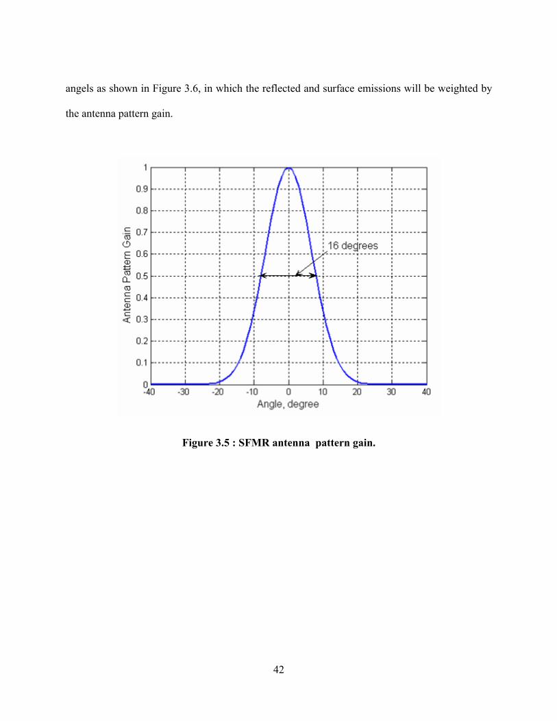
angels as shown in Figure 3.6, in which the reflected and surface emissions will be weighted by
the antenna pattern gain.
Figure 3.5 : SFMR antenna pattern gain.
42
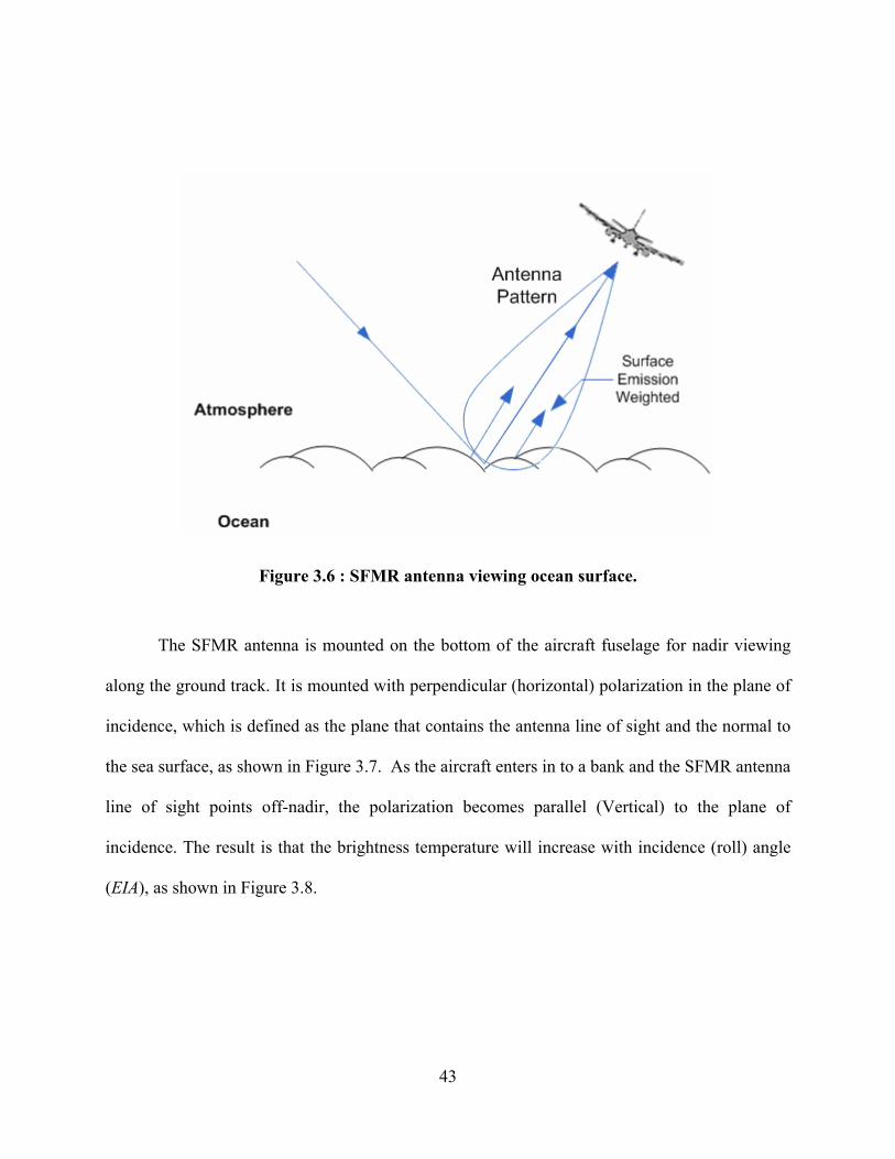
Figure 3.6 : SFMR antenna viewing ocean surface.
The SFMR antenna is mounted on the bottom of the aircraft fuselage for nadir viewing
along the ground track. It is mounted with perpendicular (horizontal) polarization in the plane of
incidence, which is defined as the plane that contains the antenna line of sight and the normal to
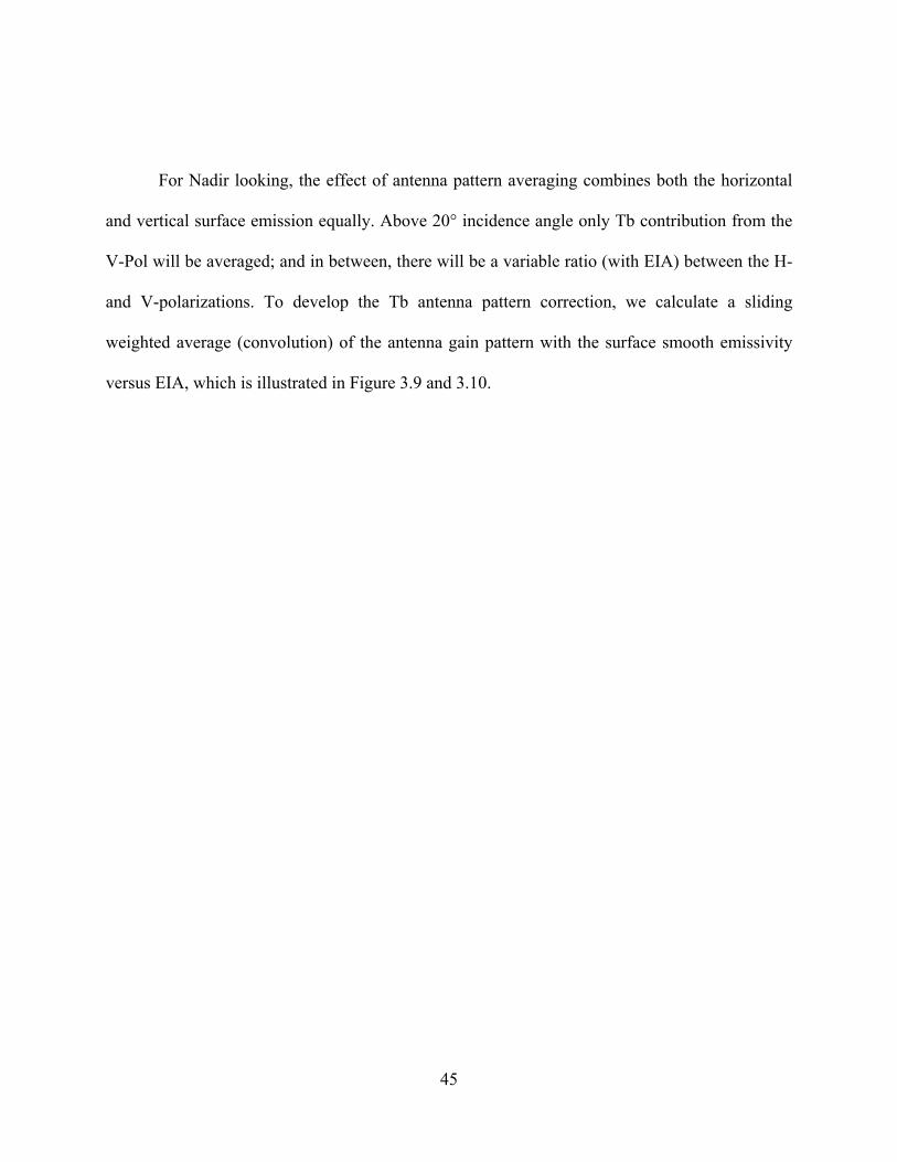
the sea surface, as shown in Figure 3.7. As the aircraft enters in to a bank and the SFMR antenna
line of sight points off-nadir, the polarization becomes parallel (Vertical) to the plane of
incidence. The result is that the brightness temperature will increase with incidence (roll) angle
(EIA), as shown in Figure 3.8.
43
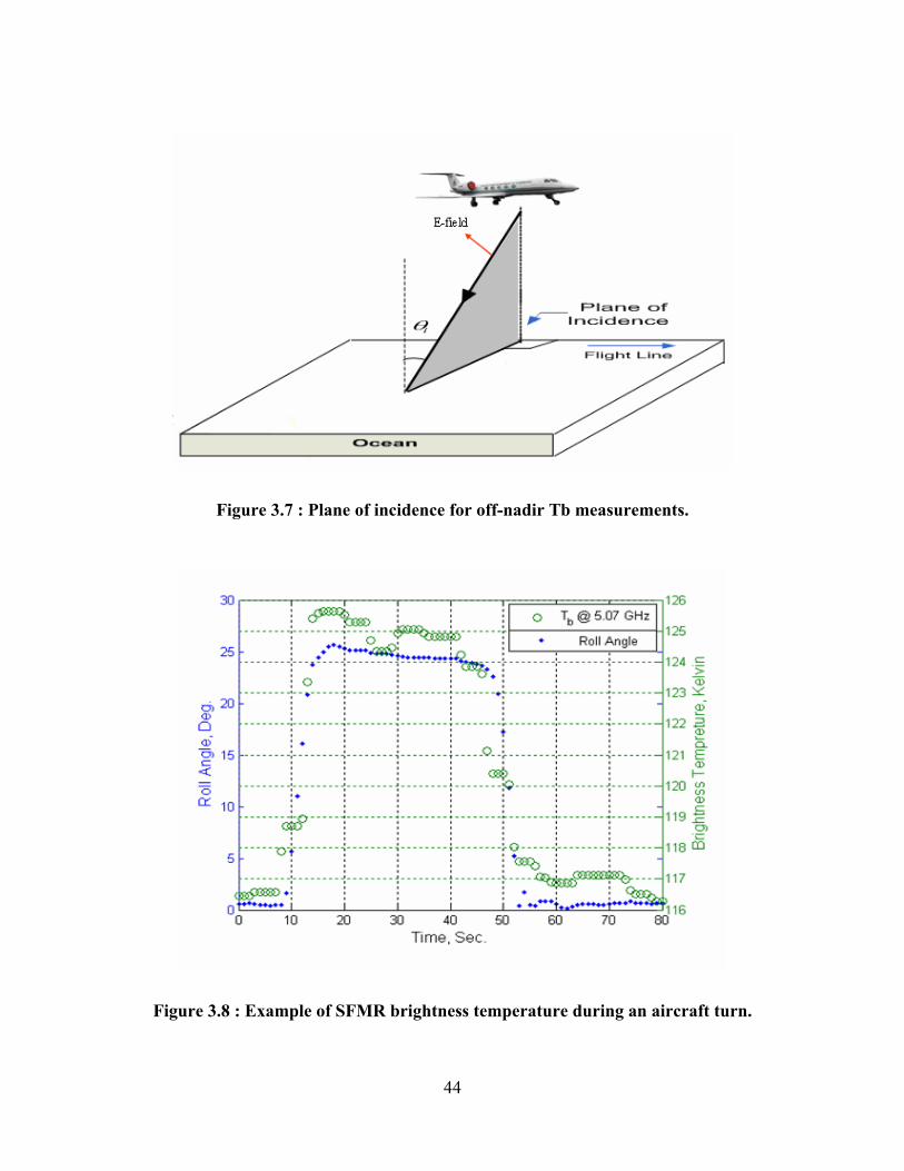
Figure 3.7 : Plane of incidence for off-nadir Tb measurements.
Figure 3.8 : Example of SFMR brightness temperature during an aircraft turn.
44
For Nadir looking, the effect of antenna pattern averaging combines both the horizontal
and vertical surface emission equally. Above 20° incidence angle only Tb contribution from the
V-Pol will be averaged; and in between, there will be a variable ratio (with EIA) between the H-
and V-polarizations. To develop the Tb antenna pattern correction, we calculate a sliding
weighted average (convolution) of the antenna gain pattern with the surface smooth emissivity
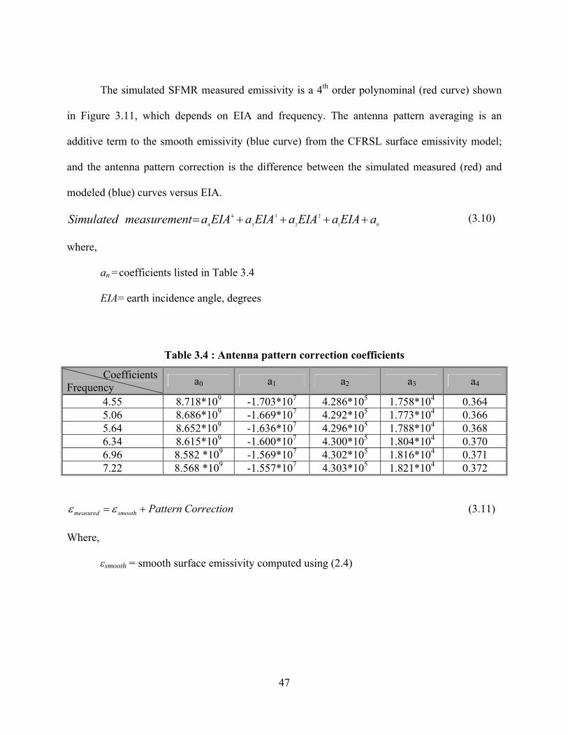
versus EIA, which is illustrated in Figure 3.9 and 3.10.
45
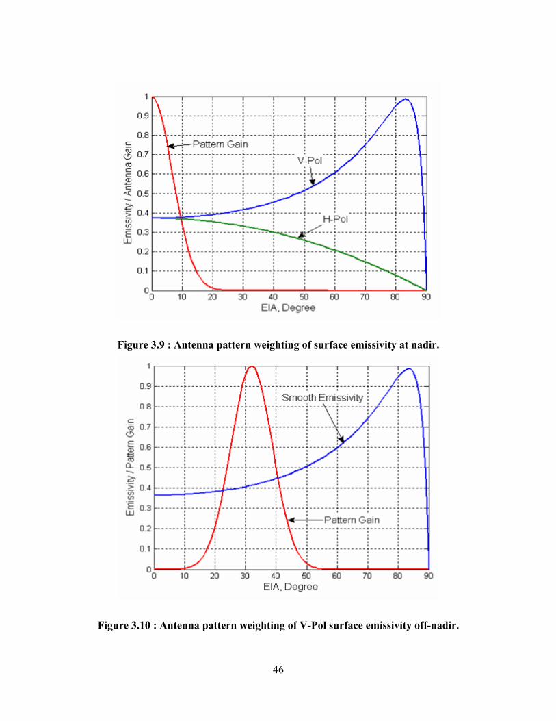
Figure 3.9 : Antenna pattern weighting of surface emissivity at nadir.
Figure 3.10 : Antenna pattern weighting of V-Pol surface emissivity off-nadir.
46
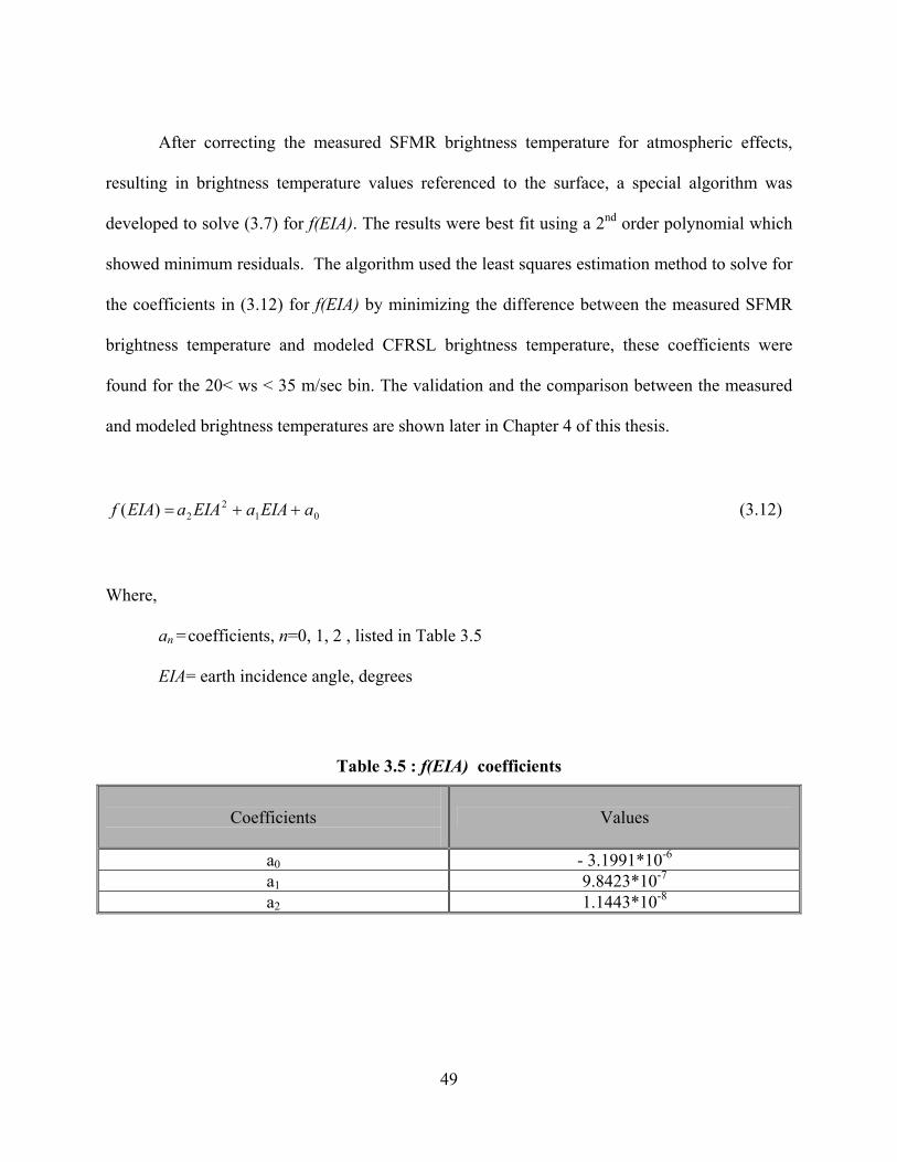
The simulated SFMR measured emissivity is a 4th order polynominal (red curve) shown
in Figure 3.11, which depends on EIA and frequency. The antenna pattern averaging is an
additive term to the smooth emissivity (blue curve) from the CFRSL surface emissivity model;
and the antenna pattern correction is the difference between the simulated measured (red) and
modeled (blue) curves versus EIA.
Simulated measurement=a4EIA4 + a3EIA3 + a2EIA2 + a1EIA+ a0 (3.10)
where,
an =coefficients listed in Table 3.4
EIA= earth incidence angle, degrees
Table 3.4 : Antenna pattern correction coefficients
Coefficients Frequency a0 a1 a2 a3 a4
4.55 8.718*109 -1.703*107 4.286*105 1.758*104 0.364 5.06 8.686*109 -1.669*107 4.292*105 1.773*104 0.366 5.64 8.652*109 -1.636*107 4.296*105 1.788*104 0.368 6.34 8.615*109 -1.600*107 4.300*105 1.804*104 0.370 6.96 8.582 *109 -1.569*107 4.302*105 1.816*104 0.371 7.22 8.568 *109 -1.557*107 4.303*105 1.821*104 0.372
CorrectionPatternsmoothmeasured += εε (3.11)
Where,
εsmooth = smooth surface emissivity computed using (2.4)
47
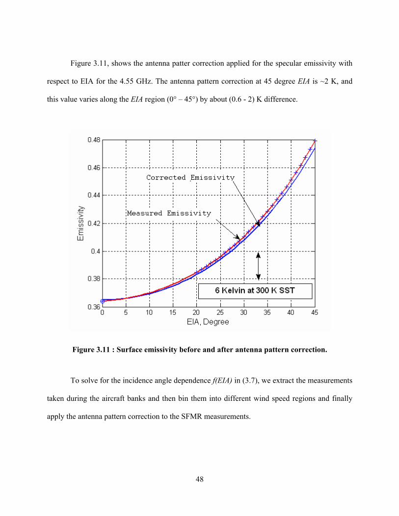
Figure 3.11, shows the antenna patter correction applied for the specular emissivity with
respect to EIA for the 4.55 GHz. The antenna pattern correction at 45 degree EIA is ~2 K, and
this value varies along the EIA region (0° – 45°) by about (0.6 - 2) K difference.
Figure 3.11 : Surface emissivity before and after antenna pattern correction.
To solve for the incidence angle dependence f(EIA) in (3.7), we extract the measurements
taken during the aircraft banks and then bin them into different wind speed regions and finally
apply the antenna pattern correction to the SFMR measurements.
48
After correcting the measured SFMR brightness temperature for atmospheric effects,
resulting in brightness temperature values referenced to the surface, a special algorithm was
developed to solve (3.7) for f(EIA). The results were best fit using a 2nd order polynomial which
showed minimum residuals. The algorithm used the least squares estimation method to solve for
the coefficients in (3.12) for f(EIA) by minimizing the difference between the measured SFMR
brightness temperature and modeled CFRSL brightness temperature, these coefficients were
found for the 20< ws < 35 m/sec bin. The validation and the comparison between the measured
and modeled brightness temperatures are shown later in Chapter 4 of this thesis.
012
2)( aEIAaEIAaEIAf ++= (3.12)
Where,
an =coefficients, n=0, 1, 2 , listed in Table 3.5
EIA= earth incidence angle, degrees
Table 3.5 : f(EIA) coefficients
Coefficients
Values
a0 - 3.1991*10-6 a1 9.8423*10-7 a2 1.1443*10-8
49
CHAPTER 4 : EMISSIVITY MODEL VALIDATIONS
The CFRSL ocean wind speed surface emissivity model, given in (3.7), has been
validated over a range of wind speed and incidence angles using SFMR data from NOAA
aircraft flights in hurricane Fabian in 2003. Comparisons to the NOAA, SFMR wind speed
retrieval algorithm provided validation at nadir incidence, and SFMR brightness temperature
measurements taken during aircraft turns provided for off-nadir validation.
4.1 SFMR Comparisons
The CFRSL wind speed surface emissivity model was validated for nadir observations by
comparisons with the NOAA/SFMR excess emissivity model. The NOAA/SFMR algorithm was
previously validated for wind speeds from 10m/sec to > 70m/sec. using dropwindsondes
measurements.
In addition to the SFMR wind speed algorithm, the Wilheit and Stogryn surface
emissivity models are often used. Figure 4.1 shows a comparison between these three with
respect to wind speed at nadir. The SFMR model is considered to be the most trusted and is the
standard for comparison because of its thorough validation. The Wilheit and Stogryn models
both have deficiencies as shown in Figure 4.1. Wilheit has two different relationships for V and
H polarizations and the two are not equal at nadir for wind speeds greater than approximately 10
m/sec, as is physically required. Plus, the V-Pol over estimates emissivity for wind speeds less
50
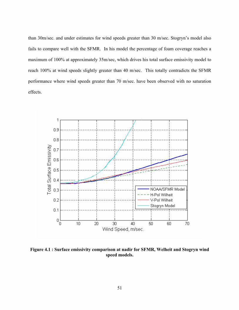
than 30m/sec. and under estimates for wind speeds greater than 30 m/sec. Stogryn’s model also
fails to compare well with the SFMR. In his model the percentage of foam coverage reaches a
maximum of 100% at approximately 35m/sec, which drives his total surface emissivity model to
reach 100% at wind speeds slightly greater than 40 m/sec. This totally contradicts the SFMR
performance where wind speeds greater than 70 m/sec. have been observed with no saturation
effects.
Figure 4.1 : Surface emissivity comparison at nadir for SFMR, Welheit and Stogryn wind speed models.
51
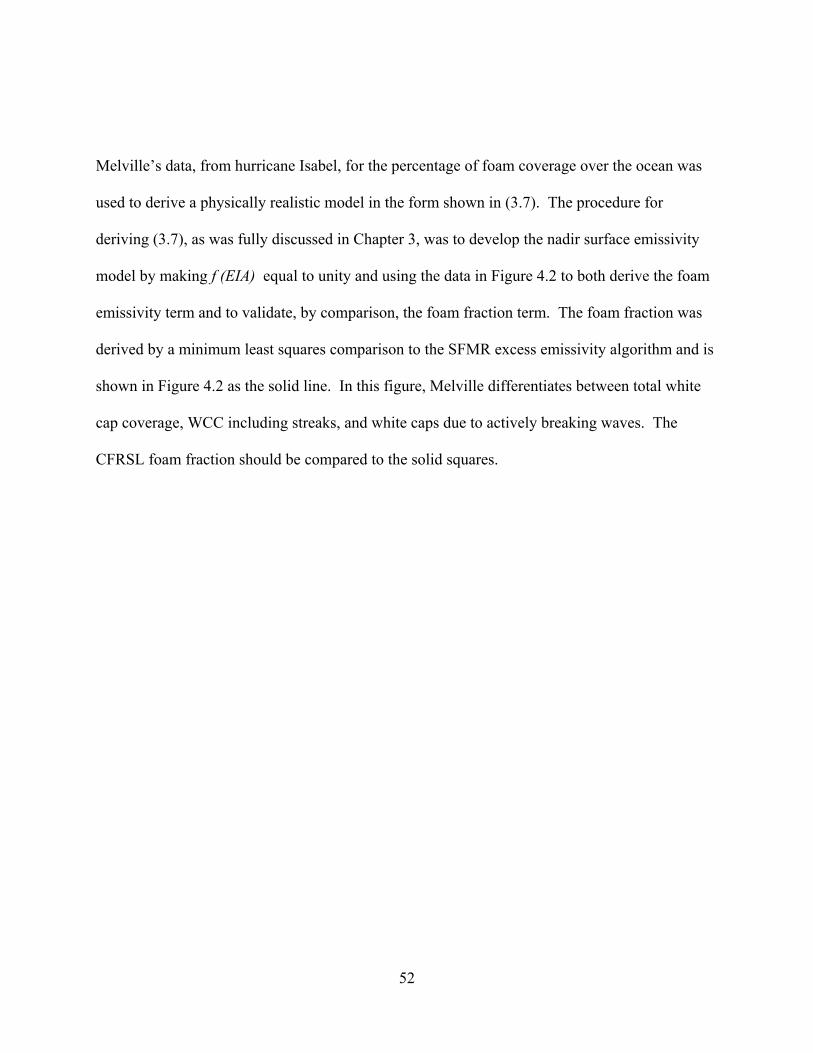
Melville’s data, from hurricane Isabel, for the percentage of foam coverage over the ocean was
used to derive a physically realistic model in the form shown in (3.7). The procedure for
deriving (3.7), as was fully discussed in Chapter 3, was to develop the nadir surface emissivity
model by making f (EIA) equal to unity and using the data in Figure 4.2 to both derive the foam
emissivity term and to validate, by comparison, the foam fraction term. The foam fraction was
derived by a minimum least squares comparison to the SFMR excess emissivity algorithm and is
shown in Figure 4.2 as the solid line. In this figure, Melville differentiates between total white
cap coverage, WCC including streaks, and white caps due to actively breaking waves. The
CFRSL foam fraction should be compared to the solid squares.
52
Figure 4.2 : Estimates of hurricane foam fraction from Melville (shown as symbols) and CFRSL foam fraction model (shown as solid line).
The nadir form for the CFRSL emissivity model was compared to the NOAA/SFMR
model in terms of brightness temperature and the results are shown in Figure 4.3. The difference
between the two models is less than half a Kelvin (0.5 K) over the whole range of wind speed
from (12-70) m/sec and for all the six SFMR frequencies. But, for the range less than 10 m/sec.
the difference is 1.1 K at the highest frequency. This is attributed to the CFRSL curve fit at
lower wind speeds for the foam fraction formula. Also, the NOAA/SFMR excess emissivity
53
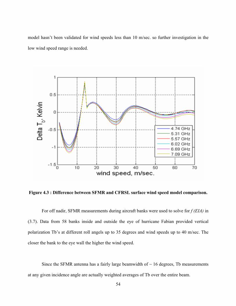
model hasn’t been validated for wind speeds less than 10 m/sec. so further investigation in the
low wind speed range is needed.
Figure 4.3 : Difference between SFMR and CFRSL surface wind speed model comparison.
For off nadir, SFMR measurements during aircraft banks were used to solve for f (EIA) in
(3.7). Data from 58 banks inside and outside the eye of hurricane Fabian provided vertical
polarization Tb’s at different roll angels up to 35 degrees and wind speeds up to 40 m/sec. The
closer the bank to the eye wall the higher the wind speed.
Since the SFMR antenna has a fairly large beamwidth of ~ 16 degrees, Tb measurements
at any given incidence angle are actually weighted averages of Tb over the entire beam.
54
Estimates for the correction due to the antenna beamwidth have been made using a weighted
average sliding window technique, or a convolution of the antenna pattern gain and the specular
emissivity model.
Corrections due to the atmospheric effect have been applied to the SFMR measurements
to be able to compare the modeled and measured surface brightness temperature by applying
some sensitivity studies to the atmosphere with different CLW, WV and Rain contents.
Brightness temperatures with rain present were not used at low wind speeds; however, most high
wind data corresponds to rainy locations and rain corrections must be used. For quality control,
measurements were inspected for radio frequency interference (RFI).
4.2 Error Estimates
Since SFMR measurements are affected by the atmosphere, which represents
approximately 10% of the total emission collected by the radiometer in the presence of light rain,
and it varies from 2 – 6 K more depending on the assumed cloud liquid water (CLW) and water
vapor (WV) levels. Care must be taken in the translation of SFMR measured brightness
temperature, at aircraft altitudes, to the ocean surface by removing the atmospheric contributions.
In this section, atmospheric error contributions to SFMR measurements were determined
and validation of the CFRSL emissivity model, by comparison to SFMR measurements
referenced to the surface, was completed for low and moderate wind speeds. Four different
hurricane atmospheres were investigated to determine the sensitivity to assumptions made.
55
The measured SFMR brightness temperature during aircraft banks have been binned
according to WS into three regions:
1. Low WS bin (0-10) m/sec
2. Medium WS bin (11-20) m/sec
3. High WS bin (> 20) m/sec.
and sensitivity studies have been conducted using the following assumed hurricane atmospheres:
1. No Atmosphere Correction Applied
2. Hurricane Atmos. (eye-wall) – W. Frank (1977)
3. Hurricane Atmos. + High CLW (eye-wall)
4. Hurricane Atmos. ( > 400Km from eye) with no clouds – W. Frank (1977).
Each of the above atmospheres has different values of atmospheric parameters that were
entered into the CFRSL RTM to remove the atmosphere effect on the measured SFMR
brightness temperature. Comparisons between the modeled (CFRSL) and measured (SFMR)
surface brightness temperature were done using the low wind speed data, with no foam present,
to evaluate the atmospheric correction using the Stogryn rough surface model, or the foam free
term in (3.7).
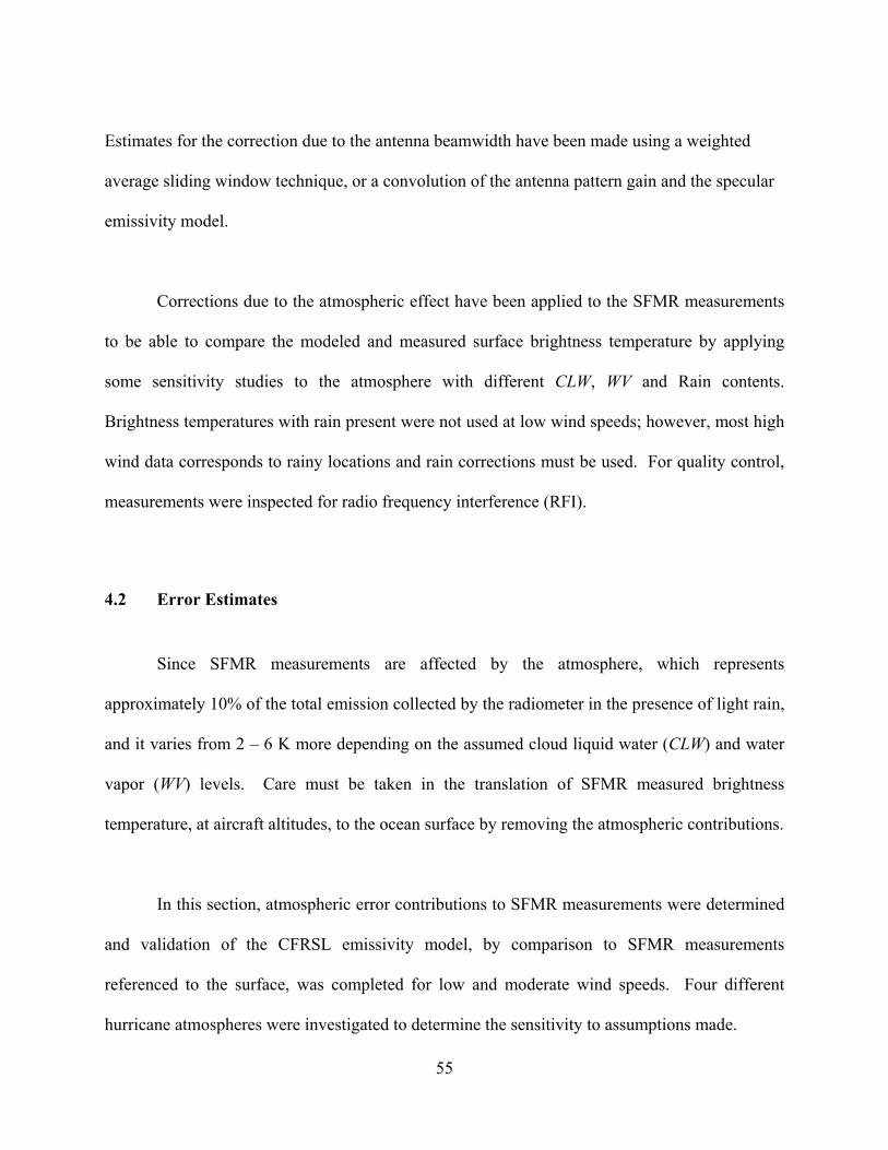
Figure 4.4 shows surface brightness temperature in Kelvin versus earth incidence angle in
degree for both measured SFMR brightness temperature and modeled CFRSL brightness
56
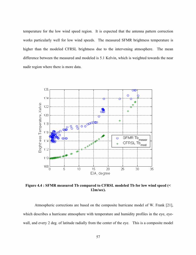
temperature for the low wind speed region. It is expected that the antenna pattern correction
works particularly well for low wind speeds. The measured SFMR brightness temperature is
higher than the modeled CFRSL brightness due to the intervening atmosphere. The mean
difference between the measured and modeled is 5.1 Kelvin, which is weighted towards the near
nadir region where there is more data.
Figure 4.4 : SFMR measured Tb compared to CFRSL modeled Tb for low wind speed (< 12m/sec).
Atmospheric corrections are based on the composite hurricane model of W. Frank [21],
which describes a hurricane atmosphere with temperature and humidity profiles in the eye, eye-
wall, and every 2 deg. of latitude radially from the center of the eye. This is a composite model
57
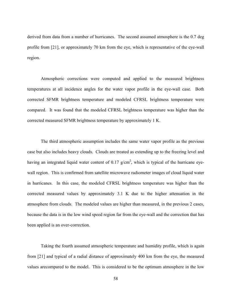
derived from data from a number of hurricanes. The second assumed atmosphere is the 0.7 deg
profile from [21], or approximately 70 km from the eye, which is representative of the eye-wall
region.
Atmospheric corrections were computed and applied to the measured brightness
temperatures at all incidence angles for the water vapor profile in the eye-wall case. Both
corrected SFMR brightness temperature and modeled CFRSL brightness temperature were
compared. It was found that the modeled CFRSL brightness temperature was higher than the
corrected measured SFMR brightness temperature by approximately 1 K.
The third atmospheric assumption includes the same water vapor profile as the previous
case but also includes heavy clouds. Clouds are treated as extending up to the freezing level and
having an integrated liquid water content of 0.17 g/cm2, which is typical of the hurricane eye-
wall region. This is confirmed from satellite microwave radiometer images of cloud liquid water
in hurricanes. In this case, the modeled CFRSL brightness temperature was higher than the
corrected measured values by approximately 3.1 K due to the higher attenuation in the
atmosphere from clouds. The modeled values are higher than measured, in the previous 2 cases,
because the data is in the low wind speed region far from the eye-wall and the correction that has
been applied is an over-correction.
Taking the fourth assumed atmospheric temperature and humidity profile, which is again
from [21] and typical of a radial distance of approximately 400 km from the eye, the measured
values arecompared to the model. This is considered to be the optimum atmosphere in the low
58
wind speed case because most of the data in this range was collected at a radial distance
approximately 400 km from the eye. At this distance from the center of the storm, clouds were
not expected to be a significant factor either.
Figure 4.5 shows surface brightness temperature in Kelvin versus earth incidence angle in
degree for both the corrected SFMR measured brightness temperature and modeled CFRSL
brightness temperature. The modeled brightness temperature is higher than the corrected
measurements but with only a small difference between the modeled and measurement of 0.87
Kelvin. This is in reasonable agreement for two reasons. First, the atmospheric assumptions
used in correcting the measured brightness temperatures to correspond to surface brightness
values are reasonable for low wind speed data, and second the difference of < 1 K is consistent
with the accuracy of the CFRSL model for wind speeds < 10 m/sec, as shown in Figure 4.3, and
represents the error contribution to total emissivity due to the foam free term. This error
contribution is then considered in the derivation of f (EIA) for higher wind speed modeling.
59
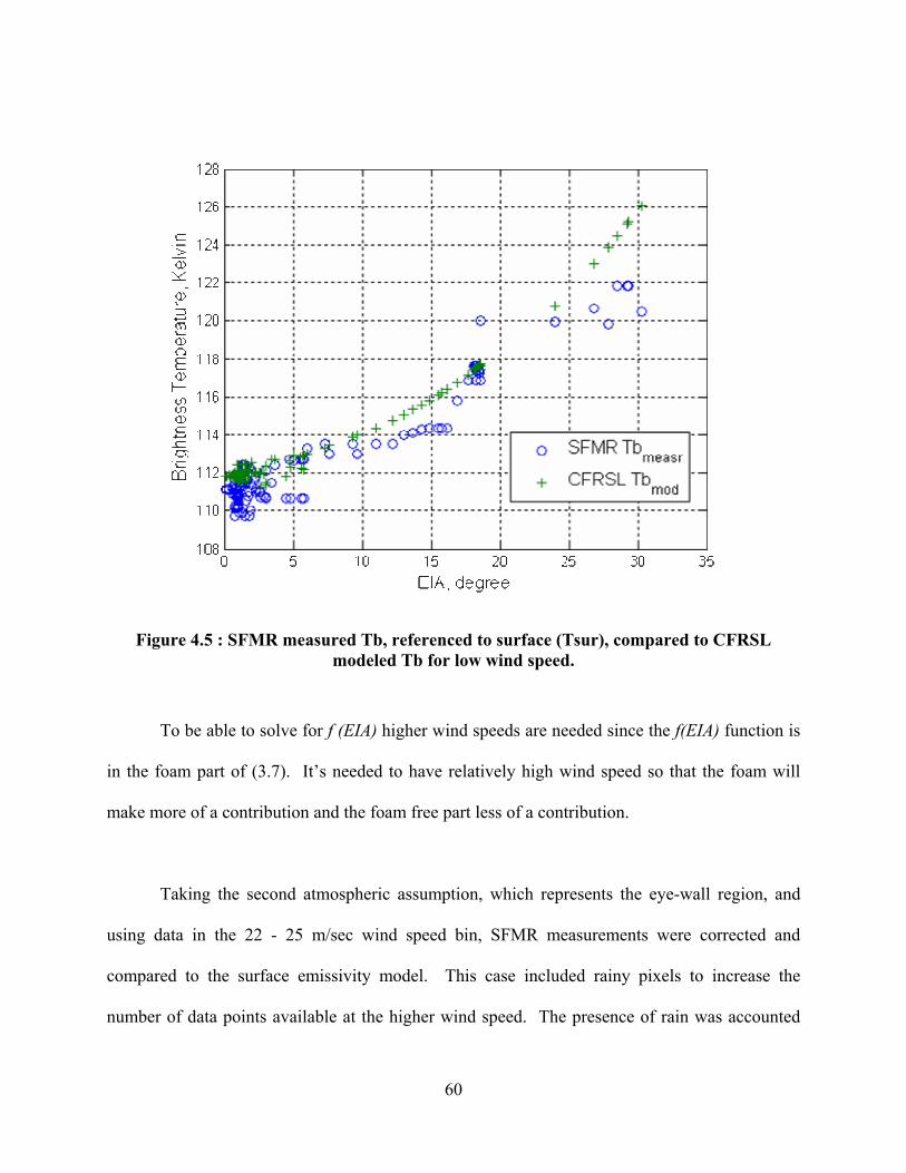
Figure 4.5 : SFMR measured Tb, referenced to surface (Tsur), compared to CFRSL modeled Tb for low wind speed.
To be able to solve for f (EIA) higher wind speeds are needed since the f(EIA) function is
in the foam part of (3.7). It’s needed to have relatively high wind speed so that the foam will
make more of a contribution and the foam free part less of a contribution.
Taking the second atmospheric assumption, which represents the eye-wall region, and
using data in the 22 - 25 m/sec wind speed bin, SFMR measurements were corrected and
compared to the surface emissivity model. This case included rainy pixels to increase the
number of data points available at the higher wind speed. The presence of rain was accounted
60
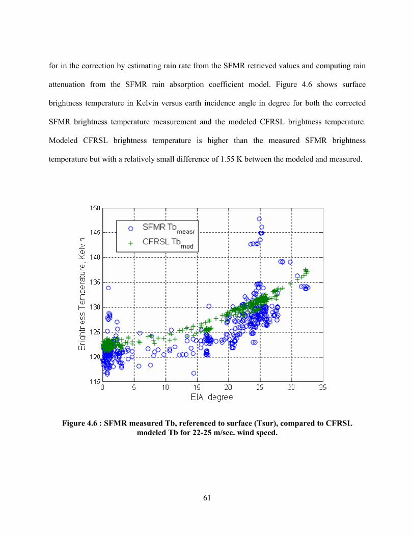
for in the correction by estimating rain rate from the SFMR retrieved values and computing rain
attenuation from the SFMR rain absorption coefficient model. Figure 4.6 shows surface
brightness temperature in Kelvin versus earth incidence angle in degree for both the corrected
SFMR brightness temperature measurement and the modeled CFRSL brightness temperature.
Modeled CFRSL brightness temperature is higher than the measured SFMR brightness
temperature but with a relatively small difference of 1.55 K between the modeled and measured.
Figure 4.6 : SFMR measured Tb, referenced to surface (Tsur), compared to CFRSL modeled Tb for 22-25 m/sec. wind speed.
61
The foam fraction corresponding to the 22-25 m/sec. bin, from Figure 4.2 , is (23 - 27) %.
Therefore, the error contribution from the foam free term is 0.7 K, leaving agreement between
modeled and measured for 22-25 m/sec. of 0.85 K. This is a measure of the error introduced by
the f (EIA) model term. Again, there is some uncertainty in the validity of the pattern correction
in the higher wind speed region.
The method for development of a high wind speed, wide swath surface emissivity model
has been described and results based on comparisons with SFMR data have shown good
matching. Agreement between measurements and modeled surface brightness temperatures to
approximately 1.5 K, or better, has been demonstrated with wind speeds up to 25 m/sec. and
incidence angles from nadir to 35 deg. Broad beamwidth antenna pattern effects were corrected
for and atmospheric contributions were accounted for in order to compare brightness
temperatures at the surface. Rain free measurements were used at low wind speeds, but at higher
wind speeds, where rain is usually present, corrections for rain effects were required.
A limited amount of data at perpendicular polarization (H-pol) exists from hurricane
flights in 2005 to begin expanding the model to both polarizations. Also, more data at higher
wind speeds is required for further analysis, and new measurements at higher incidence angles
are required to complete development out to 45 deg.
62
CHAPTER 5 : CONCLUSION
A wind speed algorithm has been developed for the design and calibration of microwave
radiometers for remotely sensing geophysical characteristics of the ocean and atmosphere in
hurricanes. It is a physically realistic model that defines the relationship between the emissivity,
or brightness temperature, of the ocean surface and the wind speed over the surface. It relies on
the increase of foam and streaks on the surface with increasing wind speed. The algorithm was
tuned to the SFMR wind speed retrieval algorithm for nadir viewing, and provides an incidence
angle dependent term derived from SFMR brightness temperature measurements in high aircraft
banks. Good agreement with the SFMR algorithm, at nadir, and with SFMR off nadir brightness
temperatures has been demonstrated.
All existing wind speed models have shortcomings in operating over a large wind speed
range and/or a large incidence angle range. The Stogryn model includes an unrealistic wind
speed/foam fraction relationship, the Wentz model does not extend to high wind speeds and is
useful over only a relatively small incidence angle range, the SFMR is for nadir viewing only,
and the Wilheit model underestimates excess emissivity by 0.1 at 70 m/sec. The CFRSL model
was designed to perform well up to greater than 70 m/sec. and out to 45 deg. Since it is physics-
based, it is adaptable to a range of instrument characteristics and measurement geometries. The
model is formulated with a foam dependent term and a foam free term. The foam term was
designed to saturate at wind speeds well beyond 70 m/sec. and to allow for frequency dispersion
63
in the model. The foam free term is intended to account for relatively low wind speed surface
roughness effects. Both terms are incidence angle dependent, but the foam term provides the
incidence angle dependence at high wind speeds.
Nadir comparisons between the CFRSL model and the SFMR model have shown good
matching. For wind speeds of approximately 15 m/sec., the modeled brightness temperature
difference between the two is less than ± 0.5 K. Also, agreement between measurements and
modeled surface brightness temperatures to approximately 1.5 K has been achieved for wind
speeds up to 25 m/sec. and incidence angles from nadir to 35 deg. These results are particularly
good considering the fact that atmospheric corrections were required and rain attenuation
corrections were required for the higher wind speed data.
Future studies will include more data in aircraft turns to enable better statistical analysis
of high wind speed and high incidence angle measurements. In order to achieve incidence angles
high enough to allow for antenna pattern correction to 45 deg. emissivity estimates, the SFMR
antenna must be mounted at approximately 25 deg. in the future. Analysis of data from the
AOC SFMR instrument is planned in order to define f(EIA) for horizontal polarization. The
AOC instrument was operational on all NOAA flights in hurricanes in 2005. These
accomplishments are all required in order to complete the wind speed model to where it can be
incorporated into the HIRA for use in HIRad studies.
HIRad is an instrument concept envisioned as an improved SFMR. It is a synthetic
aperture interferometric radiometer that provides a wide swath measurement of surface wind
64
speed and rain rate as opposed to the SFMR profile. HIRad measures out to ±45 deg. with a
swath equal to twice the aircraft altitude. This allows for the two dimensional imaging of wind
speed and rain rate for an entire hurricane in less than 4 aircraft passes from an altitude of
approximately 10 km. The improved wind speed model will be incorporated into the HIRA for
design and trade studies for HIRad. These will be conducted using wind speed and rain rate
maps for hurricane Floyd, 1999. Brightness temperature images will be computed from the
hurricane Floyd data and retrievals will be simulated for various instrument parameters over
incidence angles from 0-45 deg.
65
APPENDIX: SFMR INSTUMENT DISCRIPTION
66
The NOAA/Hurricane Research Division's (HRD) Stepped-Frequency Microwave
Radiometer (SFMR) is the prototype for a new generation of airborne remote sensing
instruments designed for operational surface wind estimation in hurricanes. It was first flown in
hurricane Allen in 1980 as reported in Jones et al. (1981) [4], Black and Swift (1984) [22] and
Delnore et al. (1985) [23]. In the mid-1980’s the instrument was redesigned and flown on the
NOAA Hurricane Research WP-3 aircraft, and the first real-time retrieval of winds on board the
aircraft in Hurricane Earl in 1985 as reported by Swift and Goodberlet (1992) [24]. The first
operational transmission of SFMR winds to TPC/NHC occurred in Hurricane Dennis in 1999.
Since 1980, the SFMR has flown on 95 flights in 30 tropical cyclones.
The concept for the first experimental SFMR was proposed by C. T. Swift and built by
NASA's Langley Research Center in 1978. The original SFMR design involved a single nadir-
viewing antenna and receiver capable of making measurements of radio emission from the sea
surface at four selectable frequencies 4.5, 5.0, 5.6, and 6.6 GHz. After 1981, the program was
transferred to the University of Massachusetts Microwave Remote Sensing Laboratory
(UMASS/MIRSL); and SFMR was updated in 1982 to six different frequencies with a better
delta-T resolution and longer integration time.
The SFMR receiver was upgraded in 1995 which allowed for increased calibration
stability, and used six different channels (4.55, 5.06, 5.64, 6.34, 6.96 and 7.22 GHz) with an
along-track nadir-viewing antenna. Since the antenna half-power beamwidth ranges from 22o to
67
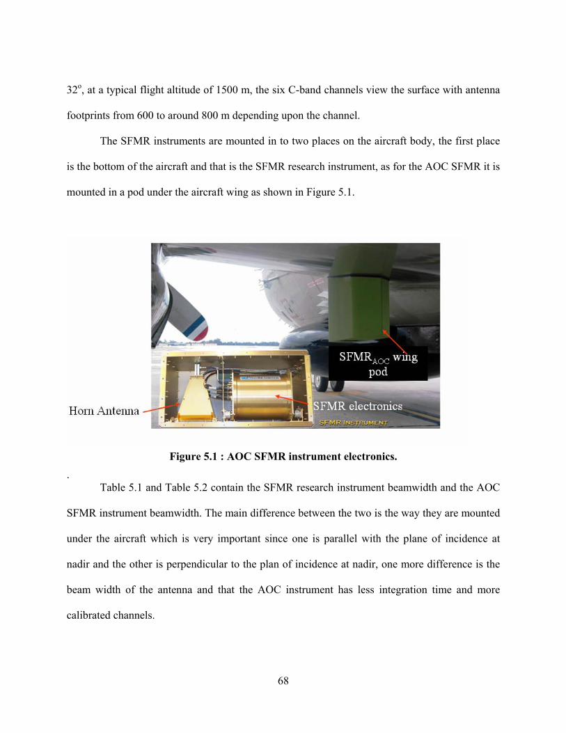
32o, at a typical flight altitude of 1500 m, the six C-band channels view the surface with antenna
footprints from 600 to around 800 m depending upon the channel.
The SFMR instruments are mounted in to two places on the aircraft body, the first place
is the bottom of the aircraft and that is the SFMR research instrument, as for the AOC SFMR it is
mounted in a pod under the aircraft wing as shown in Figure 5.1.
Figure 5.1 : AOC SFMR instrument electronics.
. Table 5.1 and Table 5.2 contain the SFMR research instrument beamwidth and the AOC
SFMR instrument beamwidth. The main difference between the two is the way they are mounted
under the aircraft which is very important since one is parallel with the plane of incidence at
nadir and the other is perpendicular to the plan of incidence at nadir, one more difference is the
beam width of the antenna and that the AOC instrument has less integration time and more
calibrated channels.
68
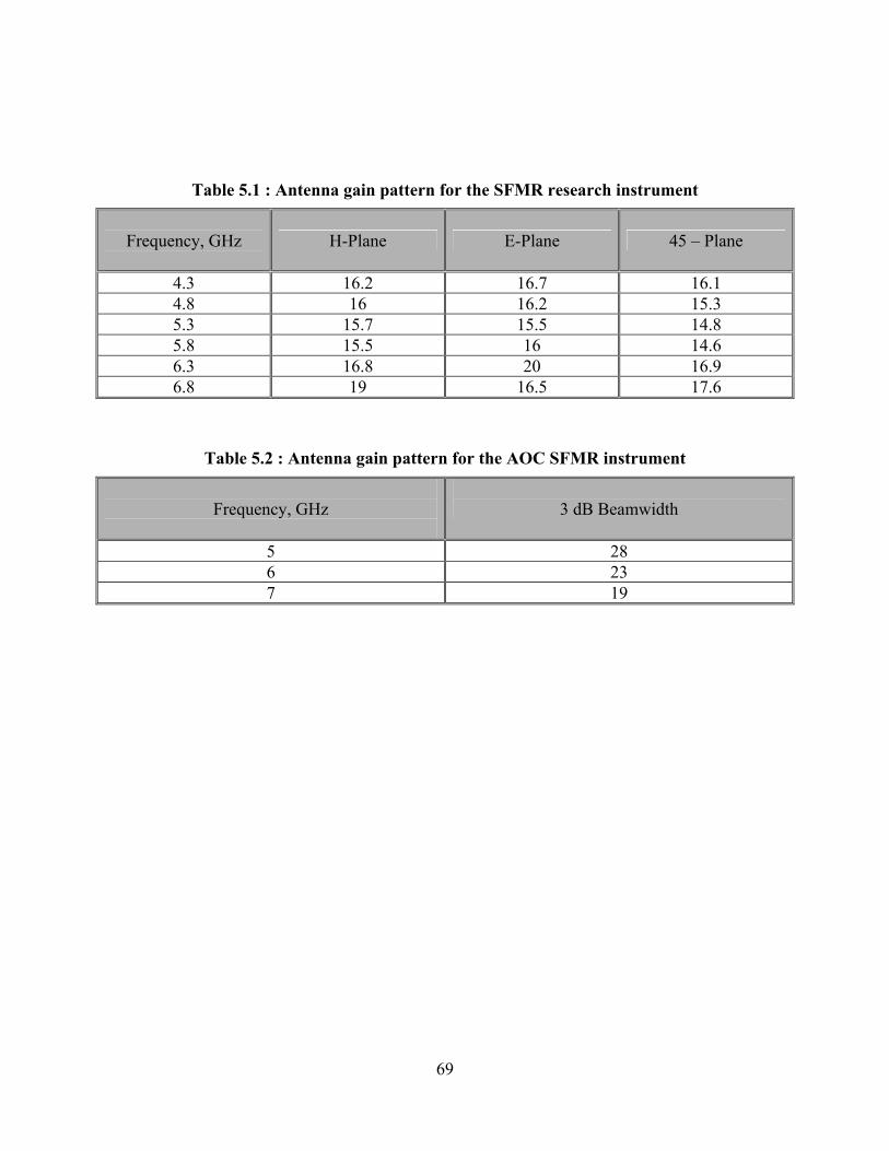
Table 5.1 : Antenna gain pattern for the SFMR research instrument
Frequency, GHz
H-Plane E-Plane 45 – Plane
4.3 16.2 16.7 16.1 4.8 16 16.2 15.3 5.3 15.7 15.5 14.8 5.8 15.5 16 14.6 6.3 16.8 20 16.9 6.8 19 16.5 17.6
Table 5.2 : Antenna gain pattern for the AOC SFMR instrument
Frequency, GHz
3 dB Beamwidth
5 28 6 23 7 19
69
LIST OF REFERENCES
[1] T. Pratt, C. Bostian, and J. Allnutt, Satellite Communications, 2nd ed: John Wiley, 2003.
[2] F. T. Ulaby, R. K. M. Moore, and A. K. Fung, Microwave Remote Sensing, Active and
Passive, vol. 1. Norwood, MA: Artech House Inc, 1981.
[3] http://www.npoess.noaa.gov/Projects/windsat.html, "WINDSAT," NOAA, 2003.
[4] W. L. Jones, P. G. Black, V. E. Delnore, and C. T. Swift, "Airborne microwave remote-
sensing measurements of Hurricane Allen," IEEE, vol. 214, pp. 275-280, 1981.
[5] E. W. Uhlhorn and P. G. Black, "Verification of Remotely Sensed Sea Surface Winds in
Hurricanes," J. Atmos. Oceanic Technol., pp. 100-115, 2003.
[6] P. Debye, "Polar Molecules," Chemical Catalog., 1929.
[7] L. A. Klein and C. T. Swift, "An improved model for the dielectric constant of sea water
at microwave frequencies," IEEE J. Oceanic Eng., vol. 2, pp. 104-111, 1977.
[8] A. Stogryn, "Equations for calculating the dielectric constant of saline water," IEEE
Trans. Micrwave Theory Tech., vol. 19, pp. 733-736, 1971.
[9] T. Meissner and F. J. Wentz., "The Complex Dielectric Constant of Pure and Sea Water
from Microwave Satellite Observations," IEEE TGARS, vol. 40, pp. 1836 - 1849, 2004.
[10] A. Stogryn, "The apparent temperature of the sea at microwave frequincies " IEEE Trans.
Antennas Propagat., vol. 15, pp. 278-286, 1967.
[11] C. S. Cox and W. H. Munk, "Measurement of the roughness of the sea surface from
photographs of the sun's glitter," J. Opt. Soc. Am., vol. 44, pp. 838-850, 1954.
70
[12] T. T. Wilheit, "A model for the microwave emissivity of the ocean's surface as a function
of wind speed," IEEE Trans. Gesoci. Electronics, vol. 17, pp. 244-249, 1979.
[13] J. P. Hollinger, "Passive micorwave measurements of sea surface roughness," IEEE
trans. of Geosci. Electron., vol. 9, pp. 165-169, 1971.
[14] J. D. Droppleman, "Apparent Emissivity of Sea Foam," Journal of Geiophysical
Research, vol. 75, pp. 696-698, 1970.
[15] A. Stogryn, "The Emissivity of Sea Foam at Microwave Frequencies," Journal of
Geiophysical Research, vol. 77, pp. 1658-1666, 1972.
[16] L. A. Rose, W. E. Asher, S. C. Reising, P. W. Gaiser, K. M. S. Germain, D. J. Dowgiallo,
K. A. Horgan, G. Farquharson, and E. J. Knapp, "Radiometric Measurements of the
Microwave Emissivity of Foam " IEEE Trans. of Geoscience and Remote Sensing, vol.
40, pp. 2619-2625, 2002.
[17] S. Padmanabhan, S. C. Reising, W. E. Asher, L. A. Rose, and P. W. Gaiser, "Effects of
foam on Ocean surface microwave emission inferred from radiometric observations of
reproducible breaking waves," IEEE Trans. of Geoscience and Remote Sensing, vol. 44,
pp. 569-583, 2006.
[18] K. Mellvile: Scripps Institute of Oceanography, 2005.
[19] J. A. Lane and J. A. Saxton, "Dielectric dispersion in pure polar liquids at very high
frequencies," Proc. Roy. Soc., vol. 3, pp. 531-545, 1952.
[20] F. Wentz and T. Meissner, "AMSR Ocean Algorithm " Remote Sensing Systems, Santa
Rosa, CA November 2 2000.
[21] W. M. Frank, "The Structure and Energetics of the Tropical Cyclone I. Storm Structure,"
Mon. Wea. Rev., vol. 105, pp. 1119-1135, 1977.
71
[22] P. G. Black and C. T. Swift, "Airborne stepped frequency microwave radiometer
measurements of rainfall rate and surface wind speed in hurricanes," presented at Second
Conf. on Radar Meteorology, Zurich, Switzerland, 1984.
[23] V. E. Delnore, G. S. Bahn, W. L. Grantham, R. F. Harrington, and W. L. Jones, "Active
and passive measurements in Hurricane Allen," NASA Tech. Rep. 1985.
[24] M. A. Goodberlet and C. T. Swift, "Passive microwave remote sensing of the ocean,"
DOC/NOAA/ERL/WPL, Boulder, CO 1992.
72