Embed Size (px)
Citation preview

Research ArticleAn Improved Maximum Power Point Approach for TemperatureVariation in PV System Applications
Abdelkhalek Chellakhi ,1 Said El Beid ,2 and Younes Abouelmahjoub 1
1National School of Applied Sciences, LabSIPE, Chouaib Doukkali University, El Jadida 24000, Morocco2CISIEV Team, Cadi Ayyad University, Marrakech 40160, Morocco
Correspondence should be addressed to Abdelkhalek Chellakhi; [email protected]
Received 3 March 2021; Accepted 9 May 2021; Published 11 June 2021
Academic Editor: Huiqing Wen
Copyright © 2021 Abdelkhalek Chellakhi et al. This is an open access article distributed under the Creative Commons AttributionLicense, which permits unrestricted use, distribution, and reproduction in any medium, provided the original work isproperly cited.
This paper develops and discusses an improved MPPT approach for temperature variation with fast-tracking speed and reducedsteady-state oscillation. This MPPT approach can be added to numerous existing MPPT algorithms in order to enhance theirtracking accuracy and response time and to reduce the power loss. The improved MPPT method is fast and accurate to followthe maximum power point under critical temperature conditions without increasing the implementation complexity. Thesimulation results under different scenarios of temperature and insolation were presented to validate the advantages of theproposed method in terms of tracking efficiency and reduction of power loss at dynamic and steady-state conditions. Thesimulation results obtained when the proposed MPPT technique was added to different MPPT techniques, namely, perturb andobserve (P&O), incremental conductance (INC), and modified MPP-Locus method, show significant enhancements of the MPPtracking performances, where the average efficiency of the conventional P&O, INC, and modified MPP-Locus MPPT methodsunder all scenarios is presented, respectively, as 98.85%, 98.80%, and 98.81%, whereas the average efficiency of the improvedP&O, INC, and modified MPP-Locus MPPT methods is 99.18%, 99.06%, and 99.12%, respectively. Furthermore, theconvergence time enhancement of the improved approaches over the conventional P&O, INC, and modified MPP-Locusmethods is 2.06, 5.25, and 2.57 milliseconds, respectively; besides, the steady-state power oscillations of the conventional P&O,INC, and modified MPP-Locus MPPT methods are 2, 1, and 0.6 watts, but it is neglected in the case of using the improvedapproaches. In this study, the MATLAB/Simulink software package was selected for the implementation of the whole PV system.
1. Introduction
The demand for electric energy has been increasing in recentyears; in this sense, there are many sources to produce it, butthere are also constraints related to its production, such asthe effect of pollution and warming global climate. Theseconstraints lead research towards the development of renew-able and nonpolluting energy sources. Photovoltaic solarenergy is certainly one of the most adequate sources ofrenewable energy [1]. Solar panels, although they are moreefficient, have yields that remain quite low. This is why wemust exploit the maximum power that they can generate byminimizing energy losses. An important feature of thesepanels is that the maximum available power is provided onlyat a single operating point called the maximum power point
(MPP), defined by a given voltage and current; this pointmoves according to the weather conditions (sunshine, ambi-ent temperature, etc.). The impact of ambient temperaturechanges on the performance and efficiency of the PV cell isone of the important effects; as a result, the PV cell’s perfor-mance and its efficiency degrade with an increase in theambient temperature. Therefore, the performance degrada-tion of the PV cell under the temperature effect can be seenin the PV cell’s characteristics, like open-circuit voltage (Voc),saturation current (Isc), fill factor (FF), and efficiency (η).According to many studies [2, 3], Voc decreases with increas-ing T whereas Isc increases slightly with increasing T. BothFF and η decrease when the ambient temperature increases,and efficiency degradation is largely due to a decrease in Voc.In addition, other parameters are affected by the temperature,
HindawiInternational Journal of PhotoenergyVolume 2021, Article ID 9973204, 21 pageshttps://doi.org/10.1155/2021/9973204

like series resistance (Rs), shunt resistance (Rsh), reverse satura-tion current density (Jo), and ideality factor (n). The variationof Rs and Rsh with temperature affects slightly the efficiency,while an exponential increase in Io with increasing T decreasesVoc rapidly. Hence, those parameters control the temperatureeffect on Voc, FF, and η of the PV cell [2].
In conclusion, when the performance of the PV celldegrades with the increase of the temperature, the powerextracted from the PV cell degrades too, and the tempera-ture variations leading to maximum power point (MPP)change. Thus, the temperature impact can be reduced bythe exploitation of the maximum power available from thePV cell.
Extracting the maximum power requires a trackingmechanism of this point called MPP tracking (MPPT) [4].Therefore, in order to harvest the maximum power outputand improve the efficiency of the entire PV system, many
maximum power point tracking (MPPT) approaches havebeen proposed in the literature [5, 6]. Perturb and observe(P&O) [7, 8] and incremental conductance (INC) [9] arethe most commonly used techniques due to their low costand easy implementation. Nevertheless, these methods showobvious drawbacks, such as low tracking efficiency undersudden variation of solar irradiation and oscillations aroundthe maximum power points (MPPs) during the steady-stateprocedure [10]. Originated from these basic methods, manymodified MPPT controllers, such as modified adaptive hillclimbing (MAHC) [11], variable step size incremental con-ductance (VSSINC) [12], and incremental resistance (INR),have been proposed. However, the dilemma between thetransient operations and amplitude of steady-state oscilla-tions has not been solved perfectly [11]. Furthermore, theimplementation of the control becomes difficult [13]. Andfurther parameters like variable step size are proposed, and
00
1
2
4
3
5
6
Curr
ent (
A)
7
8
9
5 10 15 20Voltage (V)
25 30 35 40
(a)
Voltage (V)0 5 10 15 20 25 30 35 40
200
150
100
Irrad
Temp
50
0
Pow
er (W
)
800 W/m2 at high temp1000 W/m2 at high temp
600 W/m2 at high temp400 W/m2 at high temp200 W/m2 at high temp1000 W/m2 at low temp
400 W/m2 at low temp
800 W/m2 at low temp600 W/m2 at low temp
200 W/m2 at low tempMPP
(b)
Figure 1: PV module output characteristics with different temperature variability effects and under different solar radiation levels: (a) I – Vcharacteristics and (b) P – V characteristics.
2 International Journal of Photoenergy

the optimal parameter must be determined to ensure betteraccuracy [12, 14].
Faster and more accurate MPPT algorithms, such as Betaalgorithm [15, 16], particle swarm optimization (PSO) algo-rithm [17, 18], fuzzy logic controller (FLC) algorithm [18],MPP-Locus algorithm [19], and modified MPP-Locus algo-rithm [14], have been introduced. These MPPT techniquesexhibit better effectiveness than other classical methods,especially under varying solar irradiation conditions.
In the all-existing classical and modernMPPTs, strategiesrarely take into account the temperature variation effect,which limits their performance and reduces the global effi-ciency of the PV system. Many control calculations use tem-perature as an analysis parameter to recognize MPPT. Forexample, the authors in Ref. [20] proposed a combinationof MPPT temperature calculation and PV cooling system,where the PV module temperature was utilized to calculatethe optimum voltage in order to extract the maximum powerpoint (MPP). Reference [21] presents a recent publicationnamed variable universe fuzzy logic control (VUFLC) basedon the fuzzy logic control with 25 rules. The suggestedVUFLC-temperature MPPT technique selects scalable fac-tors with respect to the dynamic variation of temperatureby combining the temperature coefficient (TC) characteristicof the PV modules in order to enhance the tracking perfor-mance [21]. The implementation complexity is the worstdrawback of the proposed VUFLC MPPT controller, wherethe fuzzy logic controller requires detailed knowledge andlarge memory for the implementation of the 25 rules.
To deal with this problem, a novel MPPT approach issuggested in this paper, which can be easily added to manyMPPT algorithms in order to improve their MPP trackingefficiency in various climatic conditions, especially undertemperature variation as explained and discussed in our pre-vious published work [22], where the proposed MPPTmethod has easily and successfully added to a previous novelpublished MPPT technique and the simulation results provethat the proposed MPPT method has significant enhance-ment of the tracking accuracy and reduction of the power
loss, without increasing the implementation complexity ofthe PV system [22].
In this context, this paper is an extension of the previouswork, in which the proposed MPPT approach has been suc-cessfully added to three MPPT algorithms, namely, P&O,INC, and modified MPP-Locus method in [14]. Different sce-nario conditions of temperature and solar irradiation areadopted to examine the performances of the improved MPPTtactic using MATLAB/Simulink environment. Based on thesimulation results, better efficiency and good accuracy havebeen obtained when using the improved MPPT approach. Inthis respect, the latter has higher tracking speed, lowersteady-state oscillation, and better power loss mitigation.
The remaining of the paper is as follows. Section 2 dis-cusses the temperature effect on the PV panel. Section 3 pre-sents theMPPTmethods. Next, theMPPT tracking efficiencyand simulation results are described in Sections 4 and 5,respectively. Finally, the conclusion of the study is reportedin Section 6.
2. Temperature Effect on the PVPanel Characteristics
The PV generator consists of numerous solar cells, where thesolar cell or PV cell is a device that converts the light energy
0
50PV m
axim
um p
ower
(W)
100
150
200
250
0 5 10 15 20 25 30 35 40 45 50 55 60 65 70 75 80Temperature (°C)
1000 W/m²800 W/m²600 W/m²
400 W/m²200 W/m²
Figure 2: Maximum power variations with temperature changes under different radiation levels.
PVarray
Rin Rout
Voltage & currentsensing
PWMgenerator
MPPT algorithm + Duty cycleadjustment
Powerconverter Load
Figure 3: Schematic diagram of the complete PV system.
3International Journal of Photoenergy

into electrical energy based on the principles of the photovol-taic effect. The PV cell performance is highly dependent ontemperature changes. The latter will affect the power energygenerated from the PV solar cells, and the PV voltage ishighly dependent on the temperature; an increase in temper-ature will decrease significantly the PV cell open-circuitvoltage [23–25].
Figure 1 shows the effect of ambient temperature on I –Vand P – V curves of the PV panel at different irradiations. Ascan be seen, the nonlinearity relation between the PV paneloutput parameters and the atmospheric variables is highlydependent on the insolation level and ambient temperaturechanges.
The PV cell short-circuit current (Isc) increases quasili-nearly with the rise of the solar radiation while the PV cellopen-circuit voltage increases slightly, and the PV cellmaximum electrical power is highly proportional to the solarradiation.
With increasing temperature, PV current increasesslightly, but PV open-circuit voltage (Voc) decreases clearlyas shown in Figure 1(a). In addition, Figure 1(b) indicatesthat the output power of the photovoltaic module decreasesrapidly with the huge increase in temperature with constantinsolation. It is noticeable from Figure 1(b) that when theambient temperature varies from a lower level to a higherlevel, the maximum output power (MPP) generated fromthe PV module under uniform radiation decreases strongly.
Figure 2 shows the temperature effect on the maximumoutput power of the PV module under different solar radia-tions, where a strong decrease in the maximum output powerin terms of the increase of temperature is noticeable. On theother hand, high temperature can affect the generated powerand the efficiency of PV cells due to the increasing internalresistance of solar cells [26].
3. Maximum Power Point Search Algorithms
The role of several MPPT techniques suggested till date is toregulate the duty ratio (d) of the DC-DC converter used inorder to extract the real MPP of the PV panel. This purposeis reached when the actual load line as seen by the PV panelmatches with that of a load at which available maximumpower is extracted from the PV panel [27]. Four conventionaltypes of DC-DC converters are mostly used for this purpose,namely, Boost, Buck, Buck-Boost, and Cuk converters. Forgrid-connected systems or for AC loads generally, an inverteris used after a DC-DC converter, but with the scientificresearch advancement, one stage is eliminated, and the DCoutput of the PV panel is directly converted to AC [28].Figure 3 shows the schematic diagram of a PV system witha DC-DC converter. Rin and Rout are the input and outputresistance seen by the DC-DC converter, respectively [27].
3.1. Principle of the P&O Method. Thanks to its simplicity,ease of implementation, and low cost, perturb and observe(P&O) MPPT technique is the most widely used in the com-mercial PV system. Its principle is based on the PV voltageperturbation regarding the comparison of the extracted PVpower [29]. If the variation of the direction is positive and
the PV output voltage increases, the MPPT technique con-tinues the perturbation in this direction; if the PV outputpower decreases, in the next perturbation, the direction willbe reversed [29].
Figure 4 shows the characteristic P –V curve, where Pmppis the MPP, P1 is to the left of the MPP, P2 is to the right ofthe MPP, and ΔU1 and ΔU2 are the changing ranges of theoutput voltage. To achieve the MPP, ΔU1 should beincreased in P1, but ΔU2 should be decreased in P2. In thiscase, ΔU1 and ΔU2 differ, and ΔU1>ΔU2. A greater dis-tance from the MPP yields a greater difference between ΔU1 and ΔU2 owing to the existence of perturbation; it is veryhard for the conventional P&O algorithm to eliminate theripple problem at the MPP. The step size of the perturbationdirectly affects the performance of the MPPT. All of these ele-ments cause power loss [29]. Figure 5 presents the flowchartof the conventional P&O method.
Pow
er (W
)
Voltage (V)
ΔU1 ΔU2P2P1
Pmpp
MPPPower
Figure 4: Tracking issues in the P – V curve.
Yes Yes
MeasureVpv(k) and Ipv(k)
Ppv(k) = Vpv(k)⁎ Ipv(k)
Ppv(k) = Ppv(k) –Ppv (k–1)
Ppv(k)>0
Vpv(k)>Vpv(k–1)
Vpv(k)>Vpv(k–1)
No
D(k+1) = D(k)+dD D(k+1) = D(k)–dD D(k+1) = D(k)+dD
YesNo
No
Start
Figure 5: Flowchart of the basic perturb and observe (P&O) tactic.
4 International Journal of Photoenergy

3.2. Principle of the INC Method. The incremental conduc-tance (INC) algorithm’s principle to track the real MPP isbased on the slope dlpv/dVpv of the PV array power curves,which is zero at the MPP, negative at the right of MPP, andpositive at the left of the MPP [13].
The maximum output powerPMPP =VMPP ∗ IMPP isobtained by differentiating the PV output power with respectto voltage and setting the result to zero:
Yes No
Yes
Yes
Start
ΔVpv = 0
D(K+1) = D(K)+dD
ΔIpv/ΔVpv>−Ipv/Vpv
D(k)(k+1) = D(k)–dD D(k+1) = D(k)+dD
YesNo
ΔIpv/ΔVpv=−Ipv/Vpv
No
ΔIpv = 0
ΔIpv
Yes
Ipv(k)=Ipv(k–1)Vpv(k)=Vpv(k–1)
ΔIpv = Ipv(k) – Ipv(k–1)ΔVpv = Vpv(k) – Vpv(k–1)
Vpv(k), Ipv(k)
Figure 6: Flowchart of the basic INC algorithm.
Update d(k+1)
Yes
Start
Is ΔPpv,ΔIpv&&ΔVpv>0Or
Is ΔPpv,ΔIpv&&ΔVpv>0True?
NoCalculated(k +1)by P&O
Flag = 0?
Flag = 0 Flag = 1
No
Yes
IsΔPpv,ΔIpv&&ΔVpv>0
d(k +1) = 1 –
d(k +1) =–1
Rupright Yes
No
Vpv(k–2)/Ipv(k)
Vpv(k–2)×[Voc–Vpv(k)]
d(k +1) = 1 –
Rupright
Vpv(k–2)/Ipv(k)
Rupright
Figure 7: Flowchart of the modified MPPT method based on theMPP-Locus technique.
Curr
ent (
A)
Voltage (V)
𝜃
Operating point
Load line 1Load line 2MPP
Figure 8: Operating point resulted by a PV module connected witha DC-DC converter.
5International Journal of Photoenergy

dPpv
dVpv= Ipv +Vpv
dIpvdVpv
= 0: ð1Þ
This leads to
dIpvdVpv
≅ΔIpvΔVpv
= −IMPPVMPP
: ð2Þ
Therefore, by evaluating the derivative, one can testwhether the PV generator is operating at near MPP or faraway from it:
dPpv
dVpv= 0
dPpv
dVpv> 0
dPpv
dVpv< 0
8>>>>>>>>><>>>>>>>>>:
9>>>>>>>>>=>>>>>>>>>;
⟶
ΔIpvΔVpv
= −IpvVpv
,
ΔIpvΔVpv
>−IpvVpv
,
ΔIpvΔVpv
<−IpvVpv
:
8>>>>>>>>><>>>>>>>>>:
9>>>>>>>>>=>>>>>>>>>;
ð3Þ
Thus, the MPP can be reached by comparing the actualconductance ðIpv/VpvÞ to the incremental conductance ðIpv/VpvÞ as shown in the flowchart given in Figure 6.
3.3. Principle of the Modified MPPT Method Based on MPP-Locus. The flowchart of this method is represented inFigure 7. Initially, after “Flag” is set as zero, the MPPTmethod uses the first condition to detect if there is an abruptinsolation variation. If there is no abrupt insolation variation,the conventional P&O MPPT algorithm will be used to trackthe MPP as shown in Figure 8 [14]. Otherwise, three equa-tions will be used to track the new MPP with a high conver-gence speed [14].
3.4. Principle of the Proposed MPPT Method
3.4.1. Characteristic of PV System with DC-DC Converter. APV module consists of numbers of solar cells connected inseries or parallel, and the total power generated is the sumof the power contributed by all of the individual solar cells.A DC-DC converter is connected in between the PV moduleand the load, as shown in Figure 9. Then, the MPPT control-ler is used to regulate the duty cycle of the DC-DC converterto ensure the load line always cuts through the I –V curve atMPP [19].
The relationships of the voltage and current of the DC-DC converter between the input and output sides areshown in
Vpv =VoutM dð Þ , ð4Þ
Ipv = Iout ∗M dð Þ, ð5Þwhere MðdÞ can be written like
M dð Þ = 11 − d
: ð6Þ
Divide (4) by (5), it can be derived as
Rin =Vpv
Ipv=
1M dð Þ2
×VoutIout
=Rout
M dð Þ2: ð7Þ
In a PV system, Equation (7) can be rewritten as
Rpv = Rin =Rout
M dð Þ2= Rload
M dð Þ2, ð8Þ
where Rpv refers to the resistance seen by the PV stringand Rload refers to the load resistance, which can be calcu-lated by substituting the duty cycle, voltage, and currentof the PV module into (8).
Rload =1
1 − dð Þ2×Vpv
Ipv: ð9Þ
Equation (17) can be defined at the instant (k) by
Rload kð Þ = 11 − d kð Þð Þ2
×Vpv kð Þ
Ipv k − 1ð Þ : ð10Þ
The relationship of the duty cycle of the boost convertercan be derived as
d = 1 −
ffiffiffiffiffiffiffiffiffiRpv
Rload
s: ð11Þ
3.4.2. The Improved MPPT Method. The improved methodidea is based on the PV panel’s I –V characteristic undertemperature variation as shown in Figures 10 and 11. Assoon as the temperature increases from 25°C to 50°C, thePV panel operating point (OP) moves from point AðVmpp1, Impp1Þ (MPP of 25°C) to point BðVðkÞ, IðkÞÞ alongwith the load line 1, where the OP is too far away frompoint EðVmpp2, Impp2Þ (MPP of 50°C) [22].
At this time, the PV panel OP is perturbed by theimproved method to point CðVðkÞ, Iðk − 1ÞÞ of the new loadresistance (load line 2), where this latter is calculated by (10).In the next step, the new duty ratio is calculated by substitut-ing the actual voltage VðkÞ, RoutðkÞ, and the previous current
Rin RoutV
A
d
L
O
A
D
PWMImproved MPPTapproach
Figure 9: Schematic diagram of the complete PV system.
6 International Journal of Photoenergy

Iðk − 1Þ, in which it is approximated the previous maximumpower point current ðImpp1Þ (MPP of 25°C) into (12), andthus, the PV panel OP operates automatically at point D ofload line 2, as can be easily shown from Figure 12 [22].
d k + 1ð Þ = 1 −
ffiffiffiffiffiffiffiffiffiffiffiffiffiffiffiffiffiffiffiffiffiffiffiffiffiffiffiffiffiffiffiffiffiffiVpv kð Þ/Ipv k − 1ð Þ
qffiffiffiffiffiffiffiffiffiffiffiffiffiffiRload kð Þ
p : ð12Þ
Finally, only a few steps by a traditional MPPT method(P&O, INC, HC, etc.) are used to track the new maximumpower point (MPP of 50°C).
Like the previous case, when the temperature suddenlydecreases, the PV panel OP moves from point EðVmpp2, Impp2Þ (MPP of 50°C) to point DðVðkÞ, IðkÞÞ alongthe load line 3. Then, the improved method perturbs theOP to point CðVðkÞ, Iðk − 1ÞðImpp2ÞÞ by calculating the resis-tance of the load line 2 using (10) and the new duty cycleusing (12). Thus, the PV panel OP operates at point B, whichis close to the new maximum power point (MPP of 25°C) as
shown in Figures 12 and 13, and finally, a few steps using atraditional MPPT method, the next MPP can be tracked [22].
Figure 14 illustrates the improved MPPT method’s flow-chart. Initially, the temperature situation is detected using therelation (13). If there is no temperature change, the P&O orINC MPPT algorithm will be used to track the MPP. Other-wise, (10) and (12) will be used to follow the new MPP with ahigh converging speed [22].
It can be concluded from [2, 30] and Figure 1 that therelations between power, voltage, and current change undertemperature variation are met as shown below:
ΔP and ΔV < 0, ΔI < 0 Temperature increases
ΔP and ΔV > 0, ΔI < 0 Temperature decreases
): ð13Þ
4. MPPT Tracking Efficiency
TheMPPT performance has become an interesting argumentfor manufacturers. However, there are no standards, whichdefine how to evaluate MPPT performance, but some pro-posals are presented in the scientific literature [30].
Voltage (V)
Load line 1
Load line 3
I(k–1)I(k)
Curr
ent (
A)
Load line 2
B(V(k),I(k))
D
E(Vmpp2,Impp2) A(Vmpp1,Impp1)
C(V(k),I((k–1))
V(k)
500C 250C
Figure 10: Operating point (OP) movement for the improved method under sudden increase of temperature.
Voltage (V)
Load line 1
Load line 2
Load line 3
I(k)I(k–1)
Curr
ent (
A)
C(V(k),I(kc1)
E(Vmpp2,Impp2) D(V(k),I(k–1))A(Vmpp1,Impp1)
B
V(k)
50 °C 25 °C
Figure 11: Operating point (OP) movement for the improved method under sudden decrease of temperature.
7International Journal of Photoenergy
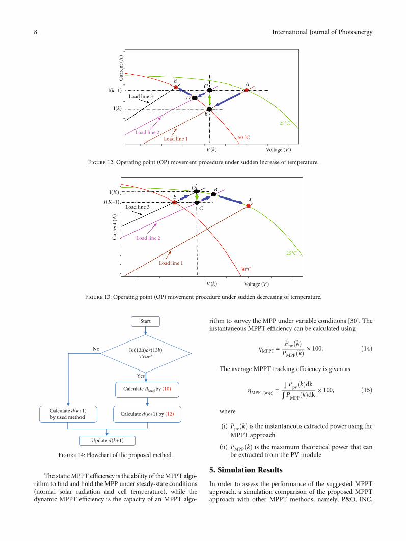
The staticMPPT efficiency is the ability of theMPPT algo-rithm to find and hold the MPP under steady-state conditions(normal solar radiation and cell temperature), while thedynamic MPPT efficiency is the capacity of an MPPT algo-
rithm to survey the MPP under variable conditions [30]. Theinstantaneous MPPT efficiency can be calculated using
ηMPPT =Ppv kð ÞPMPP kð Þ × 100: ð14Þ
The average MPPT tracking efficiency is given as
ηMPPT avgð Þ =ÐPpv kð ÞdkÐPMPP kð Þdk × 100, ð15Þ
where
(i) PpvðkÞ is the instantaneous extracted power using theMPPT approach
(ii) PMPPðkÞ is the maximum theoretical power that canbe extracted from the PV module
5. Simulation Results
In order to assess the performance of the suggested MPPTapproach, a simulation comparison of the proposed MPPTapproach with other MPPT methods, namely, P&O, INC,
Load line 1Load line 2
Load line 3
Curr
ent (
A)
I(k–1)
I(k)
D
C A
B
V(k) Voltage (V)
50 °C
25°C
E
Figure 12: Operating point (OP) movement procedure under sudden increase of temperature.
V(k)
Load line 1
Load line 2
Load line 3
E
C
D B
A
I(K)
I(K–1)
Curr
ent (
A)
50°C
25°C
Voltage (V)
Figure 13: Operating point (OP) movement procedure under sudden decreasing of temperature.
Update d(k+1)
Calculate Rload by (10)
Calculate d(k+1) by (12)
Yes
No
Calculate d(k+1)by used method
Start
Is (13a)or(13b)True?
Figure 14: Flowchart of the proposed method.
8 International Journal of Photoenergy

and the modified MPP-Locus in [14], was carried out underthe scenario of the temperature change as shown inFigure 15. The temperature rate was changed from 25°C to50°C to 40°C than from 25°C to 40°C to 50°C to 25°C; this sce-nario of temperature change was applied at constant irradia-tion: 1000W/m2, 800W/m2, and 600W/m2. To verify theperformance of the proposed method, a MATLAB/Simulinkmodel of the overall PV system shown in Figure 16 was used,which contained the PV module, boost converter, resistiveload, and an MPPT controller.
The 1Soltech 1STH-215-P is the PV panel used in thissimulation, where its electrical specifications are shown inTable 1. The main specifications for the boost converterinclude Cin = 470 μF, Cout = 47μF, L = 1 mH, andswitching frequency = 25 kHz. The load resistance was setat 10 Ω.
5.1. Comparison of the P&O Method and the P&O-IMPMethod. The simulation results of the improved P&O MPPTmethod compared with the conventional P&O MPPTmethod under the scenario of temperature with constantirradiation are shown in Figure 17. The proposed methodcan successfully track the MPP with high performance andaccuracy at the variation of temperature in different irradia-tion conditions (a) 1000W/m2, (b) 800W/m2, and (c) 600W/m2. Furthermore, thanks to its tracking mechanism, thetracking speed is significantly faster than the P&O algorithm,and it is noticeable that the improved MPPT tactic is able toreduce significantly the power losses especially at tempera-ture variation. Moreover, it is clear from Figure 17 that by
using the improved P&O MPPT method, we can reduce sig-nificantly the power loss in steady state and at temperaturevariation, especially with the increase of the temperature.There is a high amount of power loss, which is clear fromthe overshoot of power in Figure 17 when the traditionalP&O is used. On the other hand, it can be seen that the goodstability is at steady state of the PV module output power,voltage, current, and duty cycle of the boost converter in caseof using the improved P&O MPPT method, whereas nostability and fluctuation are present in the case of using theconventional P&O MPPT algorithm.
Figure 18 presents the output power and voltage stateunder steady operation. Compared with the theoretical out-put value (Pmpp and Vmpp). It can be shown that the hugeoscillations around the MPP are in a steady state when theconventional P&O MPPT method is used, while the
020
25
30
35
40
Tem
pera
ture
(°C)
45
50
0.02 0.04 0.06 0.08 0.1Time (s)
0.12 0.14 0.16 0.18 0.2
Figure 15: Scenario of temperature variation.
Continuous
[V_PV]
<I_PV>
<V_PV><V_PV>
<I_PV>[I_PV] [I_PV]
Ppv
X
Ipv
Vpv
DutyScope
[V_PV] [V_PV][P_PV]
MPPT approach
[m_Array]mIr
T
PV Array
Temp(°)
Irray (W/m2)
Ramp-up/dov
+
–
Duty [Duty]
[PWM]
[Duty] D
PWMOut+
LoadIn+
Out–In–
DC-DC boost converter
PWM
[PWM] [m_Array]P[I_PV]
Powergui
Figure 16: Schematic of the proposed PV system with MPPT algorithm.
Table 1: Parameter of the 1Soltech 1STH-215-P PVmodule at STC:temperature = 25°C and insolation = 1000 W/m2.
Parameters Value
Maximum power PMPPð Þ 213:15WVoltage at MPP VMPPð Þ 29VCurrent at MPP IMPPð Þ 7:35AOpen-circuit voltage Vocð Þ 36:3VShort-circuit current Iscð Þ 7:84ATemperature coefficient of Voc −0:36099 %/°Cð ÞTemperature coefficient of Isc 0:102 %/°Cð Þ
9International Journal of Photoenergy

0.005200120
Curr
rent
(A) V
oltta
ge (v
) Dut
y cy
cle
140Pow
er (W
)
160
180
200
205
210
215200
195
190190
200
210 200213.5
213212.5
211.5212
190
1800.01 0.015 0.06 0.065 0.07 0.116 0.12 0.14 0.145 0.185 0.19 0.195
0.040.02 0.06 0.08 0.1 0.12 0.14 0.16 0.18 0.20
Time (s)0.02 0.04 0.06 0.08 0.1 0.12 0.14 0.16 0.18 0.20
8
6
4
0.02 0.04 0.06 0.08 0.1 0.12 0.14 0.16 0.18 0.20
302520
0.02 0.04 0.06 0.08 0.1 0.12 0.14 0.16 0.18 0.20
0.5
0
P&OP&O‑IMP
(a)
Curr
ent(A
) Vol
tage
(V) D
uty
cycle
0.02 0.04 0.06 0.08 0.1 0.12 0.14 0.16 0.18 0.20
160
140
120
100
80
Pow
er (W
)
170
1650.005 0.01 0.015 0.02 0.085 0.09 0.116 0.118 0.12 0.185 0.19 0.195
170
165
160
170
165
150171
172
0.02 0.04 0.06 0.08 0.1 0.12 0.14 0.16 0.18 0.20
0.4
0.2
0
0.02 0.04 0.06 0.08 0.1 0.12 0.14 0.16 0.18 0.20
30
2025
Time (s)0.02 0.04 0.06 0.08 0.1 0.12 0.14 0.16 0.18 0.20
4.54
3.5
P&OP&O‑IMP
(b)
Figure 17: Continued.
10 International Journal of Photoenergy

improved P&O MPPT strategy presents a neglected (slight)fluctuation around the MPP with better tracking of thetheoretical output power, as well as a high power loss thatis reduced. Furthermore, the improved P&O MPPTmethod is able to reduce the time response compared to
the P&O MPPT method to 2.06 milliseconds accordingto Figure 19.
To demonstrate the effectiveness and robustness of track-ing of the proposed MPPT tactic, a calculation of thedynamic η (dyn) and static η (stat) efficiency is taken into
70
0.2
30
25
5
4
3
0.0
1290.02 0.025 0.03 0.09 0.116 0.118 0.12 0.142 0.144
129.5
130 130
116
114
118
120
110
129
128
12780
90
100
110
Pow
er (W
)Cu
rren
t(A) V
olta
ge(V
) Dut
y cy
cle
120
130
0.02 0.04 0.06 0.08 0.1
Time (s)
0.12 0.14 0.16 0.18 0.20
0.02 0.04 0.06 0.08 0.1 0.12 0.14 0.16 0.18 0.20
0.02 0.04 0.06 0.08 0.1 0.12 0.14 0.16 0.18 0.20
0.02 0.04 0.06 0.08 0.1 0.12 0.14 0.16 0.18 0.20
P&OP&O−IMP
(c)
Figure 17: Simulation result comparison between the P&O method and the P&O-IMP method under the scenario of temperature variationwith constant solar radiation: (a) 1000W/m2; (b) 800W/m2; (c) 600W/m2.
210
30
Volta
ge (V
)
29
28
211
212
Pow
er (W
) 213
Steady-state error
Pmpp
Vmpp
0.018 0.02 0.022 0.024 0.026Time (s)
0.028 0.03 0.032 0.034
0.018 0.02 0.022 0.024 0.026 0.028 0.03 0.032 0.034
P&O-IMPP&O
Figure 18: Comparison of the voltage and power in the steady state at G = 1000W/m2 and T = 25°C.
11International Journal of Photoenergy

0.006205
Pow
er (W
)
215
2.059 ms
210
0.007 0.008 0.009 0.01 0.011Time (s)
0.012 0.013 0.014 0.015 0.016
X: 0.008971Y: 212.9
X: 0.01103Y: 213.5
P&O‑IMP
MPPP&O
Figure 19: The response speed comparison for Figure 17(a).
0.02 0.04 0.06 0.08 0.10Time (s)
0.12 0.14 0.16 0.18 0.2080
85
90
Effici
ency
(%)
95
100
𝜂 (stat)‑MPPT (Avg) = 99.9%𝜂 (stat)‑MPPT (Avg) = 99.63%
𝜂 (dyn)‑MPPT (Avg) = 98.64%𝜂 (dyn)‑MPPT (Avg) = 97.92%
𝜂 (P&O)𝜂 (P&O‑IMP)
99.5100
100.5
0.02 0.025 0.03
(a)
0.02 0.04 0.06 0.08 0.10Time (s)
0.12 0.14 0.16 0.18 0.2080
85
90
Effici
ency
(%)
95
100
𝜂 (P&O) 𝜂 (stat)‑MPPT (Avg) = 99.97%𝜂 (stat)‑MPPT (Avg) = 99.81%
𝜂 (dyn)‑MPPT (Avg) = 98.64%𝜂 (dyn)‑MPPT (Avg) =9 7.92%𝜂 (P&O‑IMP)
99.699.8100
0.02 0.025 0.03
(b)
0.02 0.04 0.06 0.08 0.10Time (s)
0.12 0.14 0.16 0.18 0.2080
85
90
Effici
ency
(%)
95
100
𝜂 (P&O) 𝜂 (stat)‑MPPT (Avg) = 98.2%𝜂 (stat)‑MPPT (Avg) = 97.99%
𝜂 (dyn)‑MPPT (Avg) = 99.8%𝜂 (dyn)‑MPPT (Avg) = 99.87%𝜂 (P&O‑IMP)
99.8100
100.2
0.02 0.025 0.03
(c)
Figure 20: Efficiency profile comparison between the P&O MPPT algorithm and the improved P&O MPPT under the scenario oftemperature variation with normal solar radiation (a) 1000W/m2, (b) 800W/m2, and (c) 600W/m2.
12 International Journal of Photoenergy

0 0.02
0.005205
210
215
0.01 0.015 0.185200205
210
190 185 211212213214
190195
200
210
0.09 0.116 0.118 0.12 0.14 0.142 0.144 0.185 0.19 0.195
0.04 0.06 0.08 0.1 0.12 0.14 0.16 0.18 0.2
00
6
8
0.02
INC
0.04 0.06 0.08 0.1 0.12Time (s)
0.14 0.16 0.18 0.2
0
20
Curr
ent (
A)V
olta
ge (V
)D
uty
cycle
Pow
er (W
)
30
0.02 0.04 0.06 0.08 0.1 0.12 0.14 0.16 0.18 0.2
0
0.2
0.4
100
120
140
160
180
200
0.02 0.04 0.06 0.08 0.1 0.12 0.14 0.16 0.18 0.2
INC-IMP
(a)
0 0.02 0.04 0.06 0.08 0.1 0.12 0.14 0.16 0.18 0.2
04
56
0.02
INC
0.04 0.06 0.08 0.1 0.12Time (s)
0.14 0.16 0.18 0.2
020
Curr
ent (
A)
Volta
ge (V
)D
uty
cycle
Pow
er (W
)
3025
0.02 0.04 0.06 0.08 0.1 0.12 0.14 0.16 0.18 0.2
0
0.2
0
0.4
100
120
140
160
0.02 0.04 0.06 0.08 0.1 0.12 0.14 0.16 0.18 0.2
INC-IMP
0.185171150
160
170
160
165
170
165
170171.5
172172.5
0.116 0.118 0.120.090.0850.015 0.020.010.001 0.19 0.195
(b)
Figure 21: Continued.
13International Journal of Photoenergy
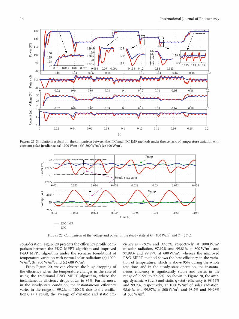
consideration. Figure 20 presents the efficiency profile com-parison between the P&O MPPT algorithm and improvedP&O MPPT algorithm under the scenario (condition) oftemperature variation with normal solar radiation: (a) 1000W/m2, (b) 800W/m2, and (c) 600W/m2.
From Figure 20, we can observe the huge dropping ofthe efficiency when the temperature changes in the case ofusing the traditional P&O MPPT algorithm, where theinstantaneous efficiency drops down to 86%. Furthermore,in the steady-state condition, the instantaneous efficiencyvaries in the range of 99.2% to 100.2% due to the oscilla-tions; as a result, the average of dynamic and static effi-
ciency is 97.92% and 99.63%, respectively, at 1000W/m2
of solar radiation, 97.92% and 99.81% at 800W/m2, and97.99% and 99.87% at 600W/m2, whereas the improvedP&O MPPT method shows the best efficiency in the varia-tion of temperature, which is above 95% during the wholetest time, and in the steady-state operation, the instanta-neous efficiency is significantly stable and varies in therange of 99.9% to 99.99%. As shown in Figure 20, the aver-age dynamic η (dyn) and static η (stat) efficiency is 98.64%and 99.9%, respectively, at 1000W/m2 of solar radiation,98.64% and 99.97% at 800W/m2, and 98.2% and 99.98%at 600W/m2.
0 0.02 0.04 0.06 0.08 0.1 0.12 0.14 0.16 0.18 0.2
Curr
ent (
A)
Volta
ge (V
)D
uty
cycle
Pow
er (W
)
03
4
520
25
30
0.02 0.04 0.06 0.08 0.1 0.12 0.14 0.16 0.18 0.2
0 0.02 0.04 0.06 0.08 0.1 0.12 0.14 0.16 0.18 0.2
20
0.2
80
90
100
110
120
130
0 0.02 0.04 0.06 0.08 0.1 0.12 0.14 0.16 0.18 0.2
0.185129
129.5
0.1450.140.120.118115
120
125
112114116118120122
0.0940.090.086127.5
128.5
129.5
128
129
0.0250.020.0150.01127128129130
0.19 0.195
(c)
Figure 21: Simulation results from the comparison between the INC and INC-IMPmethods under the scenario of temperature variation withconstant solar irradiance: (a) 1000W/m2; (b) 800W/m2; (c) 600W/m2.
0.02170.5
28.5
29
29.5
171
171.5
Pow
er (W
)Vo
ltage
(W)
172
0.022 0.024 0.026 0.028
Steady-state error
Pmpp
Vmpp
0.03 0.032 0.034
0.02 0.022 0.024
INC-IMP
0.026 0.028Time (s)
0.03 0.032 0.034
INC
Figure 22: Comparison of the voltage and power in the steady state at G = 800W/m2 and T = 25°C.
14 International Journal of Photoenergy

Time (s)2 4 6
5.254 ms
8 10 12 ×10–3
140
150
160
180
170
Pow
er (W
)
MPP
X: 0.00452Y: 172.5
X: 0.009774Y: 171.3
INC‑IMPINC
Figure 23: The response speed comparison for Figure 21(b).
0.0299
99.5100
0.025 0.03
080
85
90
95
100
Effici
ency
(%)
0.02
𝜂 (INC)
𝜂 (stat) MPPT (Avg) = 99.9%𝜂 (stat) MPPT (Avg) = 99.45%
𝜂 (dyn) MPPT (Avg) = 98.64%𝜂 (dyn) MPPT (Avg) = 97.94%
0.04 0.06 0.08 0.1 0.12Time (s)
0.14 0.16 0.18 0.2
𝜂 (INC-IMP)
(a)
0.0299.699.8100
0.025 0.03
080
85
90
95
100
Effici
ency
(%)
0.02
𝜂 (INC)
𝜂 (stat) MPPT (Avg) = 99.96%𝜂 (stat) MPPT (Avg) = 99.74%
𝜂 (dyn) MPPT (Avg) = 98.61%𝜂 (dyn) MPPT (Avg) = 98%
0.04 0.06 0.08 0.1 0.12Time (s)
0.14 0.16 0.18 0.2
𝜂 (INC-IMP)
(b)
080
85
90
95
100
Effici
ency
(%)
0.02
𝜂 (stat) MPPT (Avg) = 99.97%𝜂 (stat) MPPT (Avg) = 99.83%
𝜂 (dyn) MPPT (Avg) = 98%𝜂 (dyn) MPPT (Avg) = 97.98%
0.04 0.06 0.08 0.1
0.02
99.8
100
100.2
0.025 0.03
0.12Time (s)
0.14 0.16 0.18 0.2
𝜂 (INC)𝜂 (INC-IMP)
(c)
Figure 24: Efficiency profile comparison between the conventional INC and improved INC MPPT methods under the scenario oftemperature variation with normal solar radiation (a) 1000W/m2, (b) 800W/m2, and (c) 600W/m2.
15International Journal of Photoenergy

0.005 0.01 0.015 0.085 0.09 0.116 0.118 0.12 0.14 0.142 0.1440.015
211185190195
185190195200205
200205210215
200205210215
212213214
0.02 0.025
0120
0
20
6
8
2530
0.5
140
160
180
Pow
er (W
)Cu
ty cy
cleCu
rren
t (A
)Vol
tage
(V)
200
0.02 0.04 0.06 0.08 0.1 0.12 0.14 0.16 0.18 0.2
0 0.02 0.04 0.06 0.08 0.1 0.12 0.14 0.16 0.18 0.2
0 0.02 0.04 0.06 0.08 0.1 0.12 0.14 0.16 0.18 0.2
0 0.02 0.04 0.06 0.08 0.1 0.12 0.14 0.16 0.18 0.2
Mod-MPP-Locus
Time (s)
Mod-MPP-Locus-IMP
(a)
40
0.2
20
456
2530
0.4
60
80
100
120
140
160
Pow
er (W
)Cu
ty cy
cleCu
rren
t (A
)Vo
ltage
(V)
0.005 0.01 0.015 0.02 0.09 0.095 0.118 0.12 0.14 0.144 0.085
171
172
485052545658
155164166168170172174
164166168170172
160
165
0.19 0.195
0 0.02 0.04 0.06 0.08 0.1 0.12 0.14 0.16 0.18 0.2
0 0.02 0.04 0.06 0.08 0.1 0.12 0.14 0.16 0.18 0.2
0 0.02 0.04 0.06 0.08 0.1 0.12 0.14 0.16 0.18 0.2
0 0.02 0.04 0.06 0.08 0.1 0.12 0.14 0.16 0.18 0.2
Mod-MPP-Locus
Time (s)
Mod-MPP-Locus-IMP
(b)
Figure 25: Continued.
16 International Journal of Photoenergy

5.2. Comparison of the INC Method and the INC-IMPMethod. Figure 21 shows the simulation result for the com-parison of the INC method and the improved method INC-IMP under the scenario of temperature variation with a con-stant solar radiance: (a) 1000W/m2, (b) 800W/m2, and (c)600W/m2, where it is clear that the good performance of theimproved INCMPPT tactic provides theMPP with high accu-racy and limits the power losses at temperature variation.
From the simulation results, the improved INC MPPTmethod provides a good tracking of the MPP during the time
simulation, especially when the temperature changes, whereit can minimize significantly the power loss. On the otherhand, Figure 22 presents the comparison of the voltage andpower in the steady-state operation where better trackingperformance for the improved INC MPPT method with afew steady-state errors around the MPP is manifested. Inaddition, from Figure 23, the improved INC MPPT tacticpresents a high response speed and a better trackingaccuracy, where it can reduce the time response to 5:25milliseconds.
Pow
er (W
)Cu
ty cy
cleCu
rren
t (A
)Vo
ltage
(V)
0.01 0.015 0.02 0.086 0.09 0.118 0.12 0.122 0.14 0.1450.085
129
1295
112114116118120122
11612212540
0
20
4
3
5
2530
0.2
0.4
60
80
100
120
130
124126128130
120
118
122
0.19 0.195
0 0.02 0.04 0.06 0.08 0.1 0.12 0.14 0.16 0.18 0.2
0 0.02 0.04 0.06 0.08 0.1 0.12 0.14 0.16 0.18 0.2
0 0.02 0.04 0.06 0.08 0.1 0.12 0.14 0.16 0.18 0.2
0 0.02 0.04 0.06 0.08 0.1 0.12 0.14 0.16 0.18 0.2
Mod-MPP-Locus
Time (s)
Mod-MPP-Locus-IMP
(c)
Figure 25: Simulation results from the comparison between the modified and the improved modified MPP-Locus-IMP MPPT methodsunder the scenario of temperature variation with constant solar irradiance: (a) 1000W/m2; (b) 800W/m2; (c) 600W/m2.
Time (s)
Steady‑state error
Vmpp
Pmpp
Mod‑MPP‑Locus‑IMPMod‑MPP‑Locus
Pow
er (W
)Vo
ltage
(V)
0.02
29
29.5
30
128.8129
129.2
129.6129.8
129.4
0.022 0.024 0.026 0.028 0.0340.0320.03
0.02 0.022 0.024 0.026 0.028 0.0340.0320.03
Figure 26: Comparison of the voltage and power in the steady state at G = 600W/m2 and T = 25°C.
17International Journal of Photoenergy
125
126
127
128
129
130
0.014 0.016 0.018
2.27 ms
Time (s)
Pow
er (W
) Y: 129.4 Y: 129.5X: 0.0169 X: 0.01947
0.2 0.022 0.024 0.026
Mod‑MPP‑LocusMod‑MPP‑Locus‑IMPMPP
Figure 27: The response speed comparison for Figure 25(c).
0.02
𝜂 (Mod‑MPP‑Locus)
0.04 0.06
0.0299
99.5100
0.025 0.03
0.08 0.10Time (s)
0.12 0.14 0.16 0.18 0.2080
85
90
Effici
ency
(%)
95
100
𝜂 (Mod‑MPP‑Locus‑IMP)𝜂 (stat)‑MPPT (Avg) = 99.89%𝜂 (stat)‑MPPT (Avg) = 99.51%
𝜂 (dyn)‑MPPT (Avg) = 98.64%𝜂 (dyn)‑MPPT (Avg) = 97.96%
0.0299
99.5100
0.025 0.03
(a)
0.02 0.04 0.06
99.60.02
99.8100
0.025 0.03
0.08 0.10Time (s)
0.12 0.14 0.16 0.18 0.2080
85
90
Effici
ency
(%)
95
100
𝜂 (Mod‑MPP‑Locus) 𝜂 (stat)‑MPPT (Avg) = 99.96%𝜂 (stat)‑MPPT (Avg) = 99.74%
𝜂 (dyn)‑MPPT (Avg) = 98.61%𝜂 (dyn)‑MPPT (Avg) = 98%𝜂 (Mod‑MPP‑Locus‑IMP)
(b)
0.02 0.04 0.06
99.60.02
99.8100
100.2
0.025 0.03
0.08 0.10Time (s)
0.12 0.14 0.16 0.18 0.2080
85
90
Effici
ency
(%)
95
100
𝜂 (Mod‑MPP‑Locus) 𝜂 (stat)‑MPPT (Avg) = 99.98%𝜂 (stat)‑MPPT (Avg) = 99.83%
𝜂 (dyn)‑MPPT (Avg) = 98%𝜂 (dyn)‑MPPT (Avg) = 97.93%𝜂 (Mod‑MPP‑Locus‑IMP)
(c)
Figure 28: Efficiency profile comparison between the Mod-MPP-Locus MPPT method and the improved Mod-MPP-Locus MPPT methodunder the scenario of temperature variation with a normal solar radiation (a) 1000W/m2, (b) 800W/m2, and (c) 600W/m2.
18 International Journal of Photoenergy

Figure 24 presents the efficiency profile comparisonbetween the conventional INC and the improved INCMPPTalgorithms under the scenario of temperature change withconstant solar radiation: (a) 1000W/m2, (b) 800W/m2, and(c) 600W/m2. From Figure 24, we can observe the best track-ing efficiency of the improved INCMPPTmethod during thescenario of temperature variation and under different solarradiations, whereas the tracking efficiency of the INC MPPTalgorithm is obviously affected by the temperature change,which drops to as low as 85%. In the case of the improvedINC MPPT method, the tracking efficiency is maintainedaround 99.9% for most of the time as shown in zoomed por-tions of Figure 24, while the tracking efficiency is perturbedand shows a high fluctuation in the case of using the INCMPPT method. Furthermore, the average dynamic η (dyn)and static η (stat) efficiency of the INC MPPT method variesfrom 97.94% to 98% and from 99.45% to 99.83%, respec-tively. On the other hand, the average dynamic η (dyn) andstatic η (stat) efficiency varied from 98% to 98.64% and from99.9% to 99.97%, respectively, in the case of using theimproved INC MPPT method.
5.3. Comparison of the Modified MPP-Locus Method and theModified MPP-Locus-IMP Method. The simulation resultspresented in Figure 25 show the comparison of the Mod-MPP-Locus method and the improved Mod-MPP-LocusMPPT method under the scenario of temperature changewith different constant solar radiations 1000W/m2, 800W/m2, and 600W/m2, respectively. The results show clearlythe high tracking performance of the improved Mod-MPP-Locus MPPT method compared with the Mod-MPP-LocusMPPT method, which losses the tracking direction due totemperature change. Furthermore, the improved Mod-MPP-Locus MPPT method tracks the MPP at any tempera-ture level easily with a neglected oscillation around theMPP and the MPP is accurately reached in case of the fastchange of temperature, whereas the Mod-MPP-Locus MPPTmethod presents a high power loss due to fast temperaturechange, which is clearly observed in Figure 25 by the hugeovershoots.
Figure 26 presents the PV output power and voltage ofthe Mod-MPP-Locus MPPT method and the improvedMod-MPP-Locus MPPT method under steady-state opera-tion, compared with the theoretical output value (Pmpp and
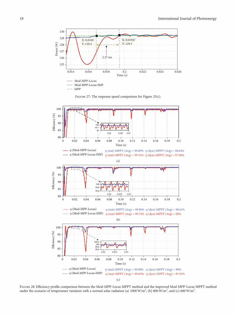
Vmpp). It is clear from Figure 26 that there exists a large oscil-lation around the theoretical output value of the power andvoltage in case of using the Mod-MPP-Locus strategy, whilethe improved Mod-MPP-Locus strategy is able to track thetheoretical output value of the power and voltage withneglected oscillations. In addition, the response time in caseof using the improved Mod-MPP-Locus is reduced to 2:57milliseconds as reported in Figure 27.
The simulation results presented in Figure 28 show theefficiency profile comparison between the Mod-MPP-LocusMPPT method and the improved Mod-MPP-Locus MPPTmethod under the scenario of temperature variation with anormal solar radiation (a) 1000W/m2, (b) 800W/m2, and(c) 600W/m2.
Due to the repeated loss of the tracking direction, we canobserve from Figure 28 the huge dropping of the efficiency attemperature changing in case of using the Mod-MPP-LocusMPPT method, where the instantaneous efficiency goes aslow as 83%. Moreover, in the steady-state condition, theinstantaneous efficiency varies in the range of 99.2% to100.2% because of the oscillations; as a result, the average ofdynamic and static efficiency varies under different solarradiations from 97.93% to 98% and from 99.51% to 99.83%,respectively. On the other hand, the improved Mod-MPP-Locus MPPT method exhibits excellent tracking efficiencyover the whole test processing, especially in the fast variationof temperature, where its instantaneous efficiency is continu-ously above 95% under all conditions. Furthermore, insteady-state operation, the instantaneous efficiency is signifi-cantly stable and varies in the range of 99.9% to 99.99%, andthe average of dynamic η (dyn) and static η (stat) efficiencyunder different irradiations is 98.64% and 99.89% at 1000W/m2, 98.61% and 99.96% at 800W/m2, and 98% and99.98% at 600W/m2, respectively.
Finally, Table 2 presents the recapitulation of all simula-tion results, which validates the effectiveness and feasibility ofthe proposed MPPT tactic.
6. Conclusion
This work proposes an improved MPPT algorithm, whichcan be easily added to other existing MPPT algorithms toenhance their tracking performance, especially under tem-perature variation. A comparative study with three MPPT
Table 2: Simulation result performance from the comparison of different MPPT control methods.
Algorithm P&O P&O-IMP INC INC-IMP Mod-Locus MPPT Mod-Locus MPPT-IMP
Tracking speed Medium Faster Medium Faster Slow Faster
Steady-state oscillation Large Small Medium Small Medium Small
Accuracy/efficiency Low High Medium High Medium High
Dynamic efficiency range (%) 97.92–97.99 98.2–98.64 97.94–98 98–98.64 97.93–98 98–98.64
Static efficiency range (%) 99.63–99.87 99.9–99.98 99.45–99.83 99.9–99.7 99.51–99.83 99.89–99.98
Time response (ms) 11.03 8.97 9.77 4.52 19.47 16.9
Power steady-state error (W) 2 Neglected 1 Neglected 0.6 Neglected
Voltage steady-state error (V) 1.5 Neglected 1 Neglected 1 Neglected
Power overshoot High Insignificant High Insignificant High Insignificant
19International Journal of Photoenergy

algorithms, namely, perturb and observe (P&O), incrementalconductance (INC), and modified MPP-Locus, has been doneunder MATLAB/Simulink software. The simulation resultsdemonstrate good contributions on the dynamic response tothe temperature variation, as well as on the steady-state per-formance, where there is a significant improvement in theresponse time, minimization of oscillation size around theMPP, and the tracking efficiency; as a result, a high amountof power loss can be significantly reduced. Furthermore, theimproved MPPT tactic can significantly enhance the trackingefficiency of the existing MPPT methods.
Data Availability
Data are available on request.
Conflicts of Interest
The authors declare that there is no conflict of interestregarding the publication of this paper.
References
[1] REN21, Renewables 2010 Global Status Report, REN21 Secre-tariat, Paris, 2010.
[2] P. Singh and N. M. Ravindra, “Temperature dependence ofsolar cell performance - an analysis,” Solar Energy Materials& Solar Cells, vol. 101, pp. 36–45, 2012.
[3] D. L. King, J. A. Kratochvil, and W. E. Boyson, “Temperaturecoefficients for PV modules and arrays: measurementmethods, difficulties, and results,” in Conference Record of theTwenty Sixth IEEE Photovoltaic Specialists Conference - 1997,Anaheim, CA, USA, 1997.
[4] S. Saravanan and B. N. Ramesh, “Maximum power pointtracking algorithms for photovoltaic system - a review,”Renewable and Sustainable Energy Reviews, vol. 57, pp. 192–204, 2016.
[5] T. Esram and P. L. Chapman, “Comparison of photovoltaicarray maximum power point tracking techniques,” IEEETransactions on Energy Conversion, vol. 22, no. 2, pp. 439–449, 2007.
[6] M. A. G. De Brito, L. Galotto, L. P. Sampaio, M. G. De Aze-vedo, and C. A. Canesin, “Evaluation of the main MPPT tech-niques for photovoltaic applications,” IEEE Transactions onIndustrial Electronics, vol. 60, no. 3, pp. 1156–1167, 2013.
[7] N. Femia, G. Petrone, G. Spagnuolo, and M. Vitelli, “Optimi-zation of perturb and observe maximum power point trackingmethod,” IEEE Transactions on Power Electronics, vol. 20,no. 4, pp. 963–973, 2005.
[8] M. A. Elgendy, B. Zahawi, and D. J. Atkinson, “Operatingcharacteristics of the P&O algorithm at high perturbation fre-quencies for standalone PV systems,” IEEE Transactions onEnergy Conversion, vol. 30, no. 1, pp. 189–198, 2015.
[9] A. Safari and S. Mekhilef, “Simulation and hardware imple-mentation of incremental conductance MPPT with direct con-trol method using cuk converter,” IEEE Transactions onIndustrial Electronics, vol. 58, no. 4, pp. 1154–1161, 2011.
[10] K. S. Tey and S. Mekhilef, “Modified incremental conductanceMPPT algorithm to mitigate inaccurate responses under fast-changing solar irradiation level,” Solar Energy, vol. 101,pp. 333–342, 2014.
[11] W. Xiao and W. G. Dunford, “A modified adaptive hillclimbing MPPT method for photovoltaic power systems,”in 2004 IEEE 35th Annual Power Electronics Specialists Con-ference (IEEE Cat. No.04CH37551), vol. 3, Aachen, Germany,2004.
[12] F. Liu, S. Duan, F. Liu, B. Liu, and Y. Kang, “A variable step sizeINC MPPT method for PV systems,” IEEE Transactions onIndustrial Electronics, vol. 55, no. 7, pp. 2622–2628, 2008.
[13] Q. Mei, M. Shan, L. Liu, and J. M. Guerrero, “A novelimproved variable step-size incremental-resistance MPPTmethod for PV systems,” IEEE Transactions on Industrial Elec-tronics, vol. 58, no. 6, pp. 2427–2434, 2011.
[14] X. Li, H. Wen, and W. Xiao, “A modified MPPT techniquebased on the MPP-locus method for photovoltaic system,” inIECON 2017 - 43rd Annual Conference of the IEEE IndustrialElectronics Society, Beijing, China, 2017.
[15] X. Li, H. Wen, L. Jiang, W. Xiao, Y. Du, and C. Zhao, “Animproved MPPT method for PV system with fast-convergingspeed and zero oscillation,” IEEE Transactions on IndustryApplications, vol. 52, no. 6, pp. 5051–5064, 2016.
[16] X. Li, H.Wen, L. Jiang, Y. Hu, and C. Zhao, “An improved betamethod with autoscaling factor for photovoltaic system,” IEEETransactions on Industry Applications, vol. 52, no. 5, pp. 4281–4291, 2016.
[17] H. Chaieb and A. Sakly, “A novel MPPT method for photovol-taic application under partial shaded conditions,” SolarEnergy, vol. 159, pp. 291–299, 2018.
[18] L. K. Letting, J. L. Munda, and Y. Hamam, “Optimization of afuzzy logic controller for PV grid inverter control using S-function based PSO,” Solar Energy, vol. 86, no. 6, pp. 1689–1700, 2012.
[19] T. K. Soon and S. Mekhilef, “A fast-converging MPPT tech-nique for photovoltaic system under fast-varying solar irradia-tion and load resistance,” IEEE Transactions on IndustrialInformatics, vol. 11, no. 1, pp. 176–186, 2015.
[20] K. Swaraj, A. Mohapatra, and S. S. Sahoo, “Combining PVMPPT algorithm based on temperature measurement with aPV cooling system,” in 2016 International Conference on Sig-nal Processing, Communication, Power and Embedded System(SCOPES), Paralakhemundi, India, 2017.
[21] Y. Wang, Y. Yang, G. Fang et al., “An advanced maximumpower point tracking method for photovoltaic systems byusing variable universe fuzzy logic control considering temper-ature variability,” Electronics, vol. 7, no. 12, p. 355, 2018.
[22] C. Abdelkhalek, E. L. B. Said, and A. Younes, “An improvedMPPT tactic for PV system under temperature variation,” in2019 8th International Conference on Systems and Control(ICSC), Marrakesh, Morocco, 2019.
[23] V. J. Fesharaki, M. Dehghani, J. J. Fesharaki, and H. Tavasoli,“The effect of temperature on photovoltaic cell efficiency,” inProceeding 1st Int Conf Emerg Trends Energy Conserv, 2011.
[24] M. K. El-Adaw, S. A. Shalaby, S. E. S. Abdl El-Ghany, andM. A. Attallah, “Effect of solar cell temperature on its photo-voltaic conversion efficiency,” International Journal of Scien-tific and Engineering Research, vol. 6, 2015.
[25] G. Li, Q. Xuan, G. Pei, Y. Su, and J. Ji, “Effect of non-uniformillumination and temperature distribution on concentratingsolar cell - a review,” Energy, vol. 144, pp. 1119–1136, 2018.
[26] A. Khatibi, F. Razi Astaraei, and M. H. Ahmadi, “Generationand combination of the solar cells: a current model review,”Energy Sci Eng, vol. 7, no. 2, pp. 305–322, 2019.
20 International Journal of Photoenergy

[27] M. A. Husain, A. Tariq, S. Hameed, A. M. S. Bin, and A. Jain,“Comparative assessment of maximum power point trackingprocedures for photovoltaic systems,” Green Energy Environ,vol. 2, no. 1, pp. 5–17, 2017.
[28] T. Ngo and S. Santoso, “Grid-connected photovoltaic con-verters: topology and grid interconnection,” J Renew SustainEnergy, vol. 6, no. 3, 2014.
[29] Y. Zhu, M. K. Kim, and H. Wen, “Simulation and analysis ofperturbation and observation-based self-adaptable step sizemaximum power point tracking strategy with low power lossfor photovoltaics,” Energies, vol. 12, no. 1, p. 92, 2019.
[30] M. Valentini, A. Raducu, D. Sera, and R. Teodorescu, “PVinverter test setup for European efficiency, static and dynamicMPPT efficiency evaluation,” in 2008 11th International Con-ference on Optimization of Electrical and Electronic Equipment,Brasov, Romania, 2008.
21International Journal of Photoenergy