Embed Size (px)
Citation preview

An Improved Deterministic Truncation of Monte Carlo Solutions
for Nuclear Reactor Analysis
December 18, 2020
Inhyung Kim and Yonghee Kim
Department of Nuclear & Quantum Engineering
Korea Advanced Institute of Science and Technology
Presented at KNS Autumn Meeting
Online, December 16-18, 2020

Monte Carlo (MC) calculation for high-fidelity reactor criticality analysis
– A stochastic method to solve a statistical problem finding out the average behavior
of the unknown parameters based on probabilistic inference
• Simulation of individual particle based on stochastic random sampling
• Calculation of reactor parameters based on statistical treatment (i.e. average and variance)
Introduction
김인형, 박사학위논문최종발표, 2020년 12월 8일
1 1i i
i
eff
S HSk
1 1( ) i i
i
eff
L T S Fk
fission rate at iteration fission rate at iteration where
fission rate at iteration 1 loss rate at iterati
on i
eff
i i
i ik
ˆ ˆ( , , ) (leakage loss term)L r E
ˆ ˆ( , , ) ( , , ) (collision loss term)tT r E r E
ˆ ˆ ˆ ˆ' ' ( , ' , ' ) ( , ', ') (scattering production term)sS d dE r E E r E ˆ ˆ ˆ' ' ( , ', ') ( , ', ') (fission production term)fF d dE r E r E
: neutron source S : transport operatorH
: neutron angular flux
(1)
( , , ) : position vectorr x y z
ˆ ( , , ) : direction vectoru v w
2

Monte Carlo (MC) calculation for high-fidelity reactor criticality analysis
– Several studies have been conducted to accelerate the calculation speed and
to reduce stochastic uncertainties more efficiently
• Coarse mesh finite difference (CMFD) method
• Modified power method
• ...
Introduction
김인형, 박사학위논문최종발표, 2020년 12월 8일
Pros Cons
High accuracy
- Direct simulation of particles’ whole
behavior
- No discretization of variables
(energy, angle, space)
- No constraints on geometry construction
High parallelization
- Parallel calculation of individual particles
Computationally expensive
- Large memory to describe explicit geometry
and to utilize cross section data
- Long time to obtain the converged source
distribution and to get quantities of interest
Uncertainties and inconsistency
- Stochastic uncertainties
- Underestimation of variance
Fundamental dilemma
- The main calculation is activated when the
FSD converges
3

Introduction
Overview
– A statistic treatment of deterministic solutions determined by FMFD-assisted MC
• To accelerate the convergence of the fission source distribution by adjusting particles’ weight
• To provide a subset of solutions to the original MC approach
ANS Winter Meeting, Online, November 16-19, 2020
MC
Particle tracking
Weight adjustment
Reactor parameters
p-FMFD & iDTMC
FMFD parameters
Eigenvalue equation
1-CMFD acceleration
MCk
MCMC
MCJ
Multiplication factor
Neutron current
Neutron flux
Group constants 1M F
k
D Diffusion coefficient
D̂ Correction factor
FMFDk Multiplication factor
FMFD Power distribution' ( / )FMFD MCw w p p
SCI
Deterministic truncation solution
Stochastic MC solution
Deterministic solutionstruncated by MC simulation
Short computing time
Fast convergence of FSD
Low uncertainty
MC-equivalent solution
(High fidelity solution)
*FMFD : Fine mesh difference method
4

Introduction
11ANS Winter Meeting, Online, November 16-19, 2020
Improved DTMC in a MC simulation
MCcalculation
Truncation
Source update
(Convergence
acceleration)
Solution
prediction
&
Variance
reduction
p-CMFD / p-FMFD iDTMC
p-CMFD (partial current based coarse mesh finite difference)
p-FMFD (partial current based fine mesh finite difference)
iDTMC (improved deterministic truncation of MC solution)
Deterministic
solution

DTMC
Deterministic truncation of MC solution method
– A conventional numerical scheme of the DTMC method
• FMFD has been applied throughout the simulation for both acceleration and variance reduction
• Instability and inconsistency problems
6김인형, 박사학위논문최종발표, 2020년 12월 8일
MCcalculation
Source update
Solution
prediction
&
variance
reduction
Deterministic
solution
Deterministic
solution
Truncation
Truncation
Inacti
ve
Acti
ve
Coupled FMFD
Coupled FMFD
DTMC
iDTMC
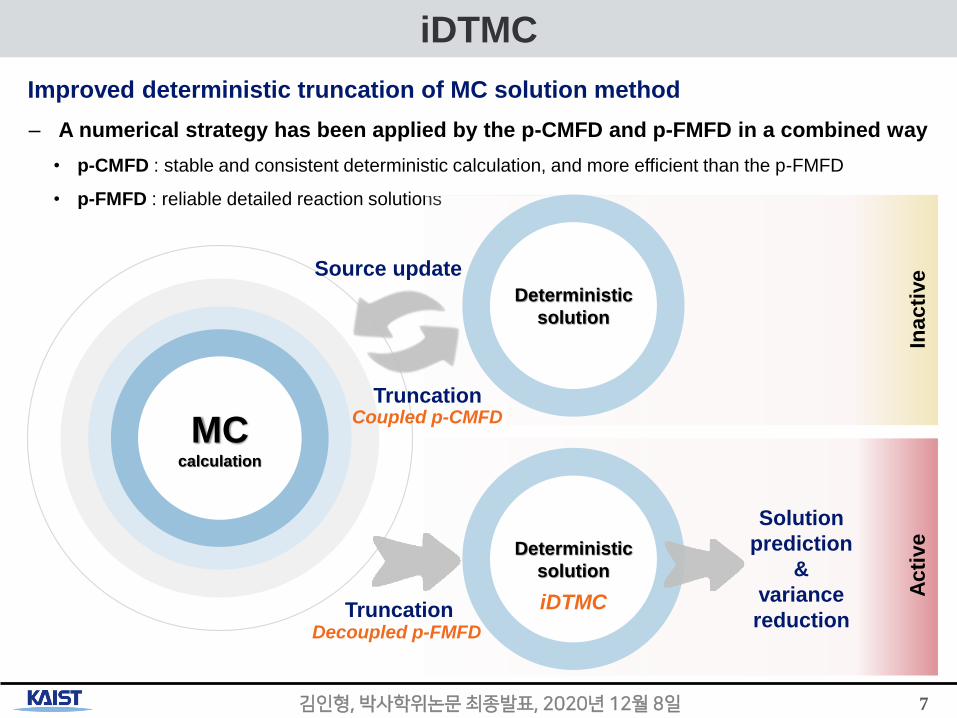
Improved deterministic truncation of MC solution method
– A numerical strategy has been applied by the p-CMFD and p-FMFD in a combined way
• p-CMFD : stable and consistent deterministic calculation, and more efficient than the p-FMFD
• p-FMFD : reliable detailed reaction solutions
7김인형, 박사학위논문최종발표, 2020년 12월 8일
MCcalculation
Source update
Solution
prediction
&
variance
reduction
Deterministic
solution
Deterministic
solution
Truncation
Truncation
Inacti
ve
Acti
ve
Coupled p-CMFD
Decoupled p-FMFD
iDTMC

iDTMC
Improved deterministic truncation of MC solution method
– Single cycle coupled p-CMFD
• A stable and consistent deterministic calculation is available even without the cycle accumulation
• The p-CMFD enables the fast convergence of the FSD
– Cycle-cumulative decoupled p-FMFD
• A stable and reliable deterministic solutions can be obtained with long cycle accumulation
• The only reliable deterministic solutions are obtained from the p-FMFD method
• Coupling is not necessary because the FSD already converged
8김인형, 박사학위논문최종발표, 2020년 12월 8일
Inactive cycle Active cycle
Single cycle coupled p-CMFDNo p-CMFD
Cycle-cumulative decoupled p-FMFD
MC
Skip
early
cycles

CMFD & FMFD
Coarse mesh finite difference (CMFD) method
– Solving the lower-order diffusion-like equation with the surface current correction
• Fast and efficient deterministic calculation
• MC-equivalent accuracy based on the generalized equivalent theory (GET)
– Unavailable to produce the detailed power distribution radial direction : assembly size (~ 20 cm)
Fine mesh finite difference (FMFD) method
– Fine mesh grid to generate the detailed pin-wise power distribution
• Radial direction : pin size (~ 1 cm)
• Axial direction : 10 – 15 cm
김인형, 박사학위논문최종발표, 2020년 12월 8일
MC CMFD grid FMFD grid
9

p-FMFD
Partial current based fine mesh finite difference (p-FMFD) method
– Neutron balance equation (diffusion-like one-group deterministic equation)
10김인형, 박사학위논문최종발표, 2020년 12월 8일
1 1 0 0
, ,
(( ) ( )) iss s s s a i i
s x y z i
aj j j j s
v
1 0
where : partial current
: absorption cross section
: no. of fission neutrons fission XS
: neutron flux
: surface area
: node volume
: surface index ( =i+1/2 and =i-1/2)
: node index
a
f
i
j
a
v
s s s
i
s
1 : fission sourcei
f ik
i1i 1i
0
1
2s i 1
1
2s i
(2)
(3)
1/2ij 1/2ij
1/2ij

One node p-CMFD
One-node CMFD acceleration
– 1-CMFD scheme is applied to accelerate the FMFD deterministic calculation
– Coarse mesh grid
• Radial direction : assembly size (~ 20 cm)
• Axial direction : 20 – 30 cm
– Fast and efficient calculation
– High parallelism
11김인형, 박사학위논문최종발표, 2020년 12월 8일
Homogenization
Correction factor
Group constants
Modulation
Source update
Global eigenvalue problemLocal fixed-source problem

Fission reaction in current generation Neutron source in next generation
Stochastic error in MC calculation
– Stochastic error cannot be exactly estimated with a single MC run
• Apparent standard deviation (SD) is underestimated due to a cycle correlation
• Variance underestimation is more critical issue in iDTMC method
because of correlation of the cycles and parameters
Methods :
김인형, 박사학위논문최종발표, 2020년 12월 8일
Fission reaction
12

Variance Estimation by Parameter Sampling
Error quantification of iDTMC method
– Overview
김인형, 박사학위논문최종발표, 2020년 12월 8일
t f
Re-sampling FMFD parameters
Perturbed eigenvalue calculation
Variance estimation
MC simulation
PDFs of FMFD parameters
13
a

Variance Estimation by Parameter Sampling
Error quantification of iDTMC method
– Flow chart
김인형, 박사학위논문최종발표, 2020년 12월 8일 14
FMFD parameters sampling
URN generation
Neutron flux
Cross sections
1st PT for eigenvalue
Direct calculation for pin power

Variance Estimation by Parameter Sampling
Error quantification of iDTMC method
– FMFD parameters to calculate keff
• Group constants (cross sections) are calculated from MC simulation every cycle
김인형, 박사학위논문최종발표, 2020년 12월 8일
Inactive cycle Active cycle
MC
Skip cycle
1xGroup constants 2x 3x 4x 5x 6x 7x 8x 9x
Average 1x 2x 3x 4x 5x 6x 7x 8x 9x
15
Resampling of cross sections• Resampling parameters include cross sections and flux
(i.e. total, absorption, and fission cross sections)
• Current are just taken from the MC simulation as a solution
to preserve the nodal balance by a reference
Variance Estimation by Parameter Sampling
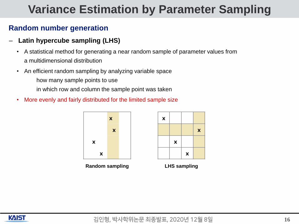
Random number generation
– Latin hypercube sampling (LHS)
• A statistical method for generating a near random sample of parameter values from
a multidimensional distribution
• An efficient random sampling by analyzing variable space
how many sample points to use
in which row and column the sample point was taken
• More evenly and fairly distributed for the limited sample size
김인형, 박사학위논문최종발표, 2020년 12월 8일
x
x
х
x
х
х
х
х
Random sampling LHS sampling
16

Variance Estimation by Parameter Sampling
Correlation sampling
– Correlation matrix
• Correlation between total, absorption and nu X fission cross section
• Correlation coefficient can be calculated by
• Correlation matrix can be composed as the follows
– Cholesky decomposition
• Correlation matrix C (positive-definite) is decomposed to be a form of
• Positive definiteness should be improved for pseudo non-positive definite due to stochastic uncertainty
김인형, 박사학위논문최종발표, 2020년 12월 8일
,
cov( , )X Y
X Y
X Y
, , ,
, , ,
, , ,
t t t a t f
a t a a a t
f t f a f f
TC LL
C
' 0.1 I C C
17
at f
t
a
f

Variance Estimation by Parameter Sampling
Correlation sampling
– Conversion by inverse cumulative density function (CDF)
• Underlying function is assumed to be a normal distribution
• Random parameters can be obtained by the uniform random number (URN) calculated from LHS
– Correlated parameters generation
• Correlated parameters can be generated by multiplying the Cholesky-decomposed lower triangular
matrix and the matrix for random parameters calculated by LHS
– Correlated URN
• Correlated parameters are again converted to be URNs
• Correlated URNs can be obtained by the CDF conversion
김인형, 박사학위논문최종발표, 2020년 12월 8일
G L P
312 ( ) sNp erf P
where : error function
: URN [0,1)
erf
18
(3 ) (3 3) (3 )s sN N
1' 1
2 2
gerf
: element of matrix where g G

Variance Estimation by Parameter Sampling
Correlation sampling
– Correlated cross section sampling
• Using the correlated URNs, the correlated cross sections can be sampled
• In the sampling of the cross section, the probability function is created by the FMFD parameters
PDF made from the FMFD parameters does not follow the normal distribution
• The cross sections are directly sampled from the actual given PDF
김인형, 박사학위논문최종발표, 2020년 12월 8일
1 2 3 4 5 6 7 8 9
1 2 3 4 5 6 7 8 9
CDF
19

Variance Estimation by Parameter Sampling
Eigenvalue calculation by 1st order perturbation theory
– 1st order perturbation theory
• Multiplication factor can be easily calculated with the perturbed parameters
– Forward and adjoint fluxes are different in the p-FMFD method due to the correction factors
– But they are comparable each other with some reasons
– Therefore, the self-adjointness is assumed in 1st PT error quantification
김인형, 박사학위논문최종발표, 2020년 12월 8일
*
*
( ,[ ] )1 1
' ( , )k k
F M
F
*
1where
, : unperturbed matrices
: unperturbed reference eigenvalue
: unperturbed flux (forward flux)
: adjoint flux
, : perturbed and
k
k
M F
M F M F
20
(36)
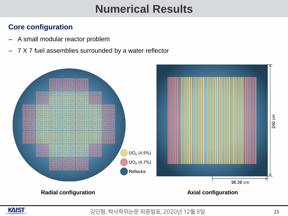
Numerical Results
Core configuration
– A small modular reactor problem
– 7 X 7 fuel assemblies surrounded by a water reflector
21김인형, 박사학위논문최종발표, 2020년 12월 8일
Radial configuration Axial configuration

Numerical Results
Calculation condition
– Total 112 cores of Xeon E5-2697 with clock speed of 2.60 GHz
– Skip p-CMFD : 1
– Skip early cycles : 5
– According to SCI
• Minimum generation size = 6,000,000 histories per cycle
• The number of inactive cycles were automatically determined
– 10 active cycles were used
– For real standard deviation, 20 independent runs simulated with different random seeds
– Reference solution : 1.27774 ± 1.2 pcm
• No. of histories : 6,000,000
• No. of inactive cycles 120
• No. of active cycles : 500
• No. of batches : 2
22김인형, 박사학위논문최종발표, 2020년 12월 8일
6,266,098 ≅ 6,000,000× =213,860
Total number of fine nodes
5.86
No. of neutrons Optimum generation size
0.2
Off-peaking
/

Numerical Results
FMFD parameters
– Three pin positions are arbitrarily selected to characterize the FMFD parameters
23김인형, 박사학위논문최종발표, 2020년 12월 8일

Numerical Results
FMFD parameters
– Convergence behavior; central region (62,59,10)
24김인형, 박사학위논문최종발표, 2020년 12월 8일

Numerical Results
FMFD parameters
– Convergence behavior; peripheral region (52,24,10)
25김인형, 박사학위논문최종발표, 2020년 12월 8일

Numerical Results
FMFD parameters
– PDF and CDF; non-central region (62,59,10)
26김인형, 박사학위논문최종발표, 2020년 12월 8일
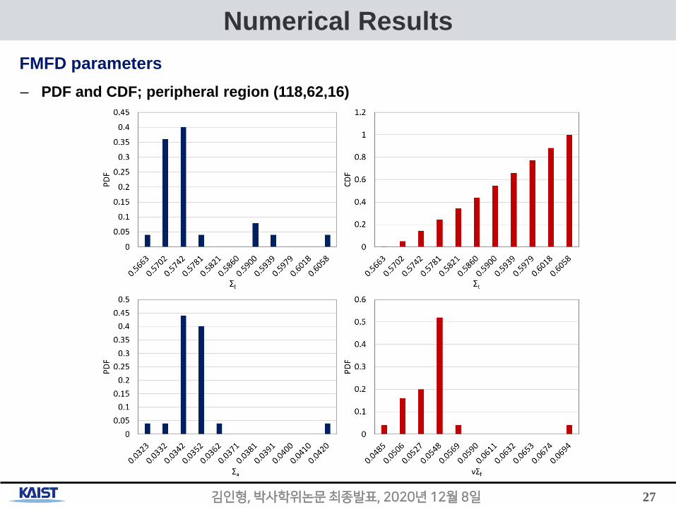
Numerical Results
FMFD parameters
– PDF and CDF; peripheral region (118,62,16)
27김인형, 박사학위논문최종발표, 2020년 12월 8일

5.5
6
6.5
7
7.5
8
8.5
9
0 20 40 60 80 100
Stan
dar
d d
evia
tio
n (
pcm
)
No. of perturbed samples
Direct calculation
1st PT (standard)
Computing time of 1st PT vs. direct calculation for 100 samples
Numerical Results
1st PT vs. direct calculation
– The number of samples
28김인형, 박사학위논문최종발표, 2020년 12월 8일
1st PT Direct
Time (sec.) 4.7 158.8

Numerical Results
FSD convergence
– By the Shannon entropy
29김인형, 박사학위논문최종발표, 2020년 12월 8일
8.3
8.35
8.4
8.45
8.5
8.55
8.6
0 10 20 30 40 50 60 70 80 90
Shan
no
n e
ntr
op
y
Cycle (inactive + active)
Standard MC
MC-CMFD
64 cycles

Numerical Results
Multiplication factor & stochastic errors
30김인형, 박사학위논문최종발표, 2020년 12월 8일
ParameterCycle
1 3 10 15 20
MC-CMFD
keff 1.27706 1.27763 1.27781 1.27782 1.27778
σa - 18.3 13.0 9.9 8.9
σr 46.4 24.2 13.7 13.4 11.3
iDTMC
keff 1.27777 1.27776 1.27776 1.27775 1.27775
σa - 0.6 0.5 0.5 0.5
σr 5.7 5.7 5.2 4.9 4.8
1st PT 6.4 6.6 6.0 5.5 5.2
* 1.27774 1.2 pcmref
effk

0
5
10
15
20
25
30
35
40
45
50
0 2 4 6 8 10
Rea
l sta
nd
ard
dev
iati
on
Active cycle
MC-CMFDiDTMC
Numerical Results
Real standard deviation of the multiplication factor
31김인형, 박사학위논문최종발표, 2020년 12월 8일
6.4 times
5.2 times
Much more reliable solutions can be obtained with the iDTMC method
Remind that the iDTMC method is designed to pursue the early truncation

Numerical Results
Comparison of standard deviation
– iDTMC vs. 1st PT
32김인형, 박사학위논문최종발표, 2020년 12월 8일
They show great agreement each other throughout the simulation
The reliable stochastic error can be calculated with a single batch calculation
5.4
5.6
5.8
6.0
6.2
6.4
6.6
6.8
7.0
0 2 4 6 8 10
Stan
dar
d d
evia
tio
n
Active cycle
iDTMC
1st PT

Numerical Results
Real standard deviation of the 2D pin power
– At cycle 1
33김인형, 박사학위논문최종발표, 2020년 12월 8일
MC-CMFD iDTMC
2
, , ,
1( )
bNb
i j i j i j
bb
p pN
where : batch number, : No. of batchesbb N
Cycle 1 MC-CMFD iDTMC
Avg. 0.058 0.011
(39)

Numerical Results
Real standard deviation of the 2D pin power
– At cycle 10
34김인형, 박사학위논문최종발표, 2020년 12월 8일
MC-CMFD iDTMC
2
, , ,
1( )
bNb
i j i j i j
bb
p pN
where : batch number, : No. of batchesbb N
Cycle 10 MC-CMFD iDTMC
Avg. 0.019 0.009
(40)

Numerical Results
Real standard deviation of the 2D pin power
– At cycle 10
35김인형, 박사학위논문최종발표, 2020년 12월 8일
iDTMC Parameter sampling
2
, , ,
1( )
bNb
i j i j i j
bb
p pN
where : batch number, : No. of batchesbb N
Cycle 10 iDTMC Direct
Avg. 0.009 0.009
(40)

Numerical Results
Relative error distribution for the 2D pin power
– At cycle 1
36김인형, 박사학위논문최종발표, 2020년 12월 8일
MC-CMFD iDTMC*
, ,
, *
,
100 (%) i j i j
i j
i j
p p
p
* where : reference pin powerp
Error (%) MC-CMFD iDTMC
Avg. 3.2 0.8
Max. 32.2 7.5
(41)
(%)

Numerical Results
Relative error distribution for the 2D pin power
– At cycle 10
37김인형, 박사학위논문최종발표, 2020년 12월 8일
MC-CMFD iDTMC*
, ,
, *
,
100 (%) i j i j
i j
i j
p p
p
* where : reference pin powerp
Error (%) MC-CMFD iDTMC
Avg. 1.0 0.6
Max. 9.6 5.6
(42)
(%)

Numerical Results
Computing time
– Deterministic calculation
– MC calculation
38김인형, 박사학위논문최종발표, 2020년 12월 8일
Methods p-CMFDp-FMFD
w/o one-node p-CMFD w/ one-node p-CMFD
Time (sec.) 0.03 97.9 1.4
Standard MC MC-CMFD iDTMC
No. of inactive cycles 81 23.1 23.1
No. of active cycles 10 10 10
Inactive time (hr.) 1.2 0.7 0.8
Active time (hr.) 0.29 0.29 0.51
Total time (hr.) 1.47 0.95 1.29
p-FMFD for solution prediction
Variance estimation

0
5
10
15
20
25
30
35
40
45
0.0E+0
1.0E+4
2.0E+4
3.0E+4
4.0E+4
5.0E+4
6.0E+4
7.0E+4
8.0E+4
9.0E+4
1.0E+5
1 2 3 4 5 6 7 8 9 10
FOM
rat
io (
iDTM
C/M
C-C
MFD
)
FOM
Active cycle
MC-CMFD
iDTMC
FOM ratio
Numerical Results
FOM for the multiplication factor
39김인형, 박사학위논문최종발표, 2020년 12월 8일
2
1FOM
T 2where : time (sec), : varianceT
42 times higher

Numerical Results
APR1400 quarter core problem
– 1st cycle fuel loading pattern
– 241 fuel assemblies
– Fuel zoning & Bas are modelled
40김인형, 박사학위논문최종발표, 2020년 12월 8일
Radial configuration Axial configuration
Type A0 (1.71)
Type B3, C2 (3.64+3.14)
Type C3 (3.64+3.14)
Type C0 (3.64+3.14)
Type B1, C1
(3.14+2.64)
Type B2 (3.14+2.64)

Numerical Results
Calculation condition
– Total 112 cores of Xeon E5-2697 with clock speed of 2.60 GHz
– Skip p-CMFD : 1
– Skip early cycles : 5
– According to the SCI
• Minimum generation size = 6,000,000 histories per cycle
• The number of inactive cycles were automatically determined
– 10 active cycles were used
– For real standard deviation, 30 independent runs simulated with different random seeds
– Reference solution : 1.20392 ± 0.82 pcm
• No. of histories : 10,000,000
• No. of inactive cycles 60
• No. of active cycles : 300
• No. of batches : 4
41김인형, 박사학위논문최종발표, 2020년 12월 8일
17,173,081 ≅ 20,000,000× =586,112
Total number of fine nodes
5.86
No. of neutrons Optimum generation size
0.2
Off-peaking
/

Numerical Results
FSD convergence behavior
42김인형, 박사학위논문최종발표, 2020년 12월 8일
10.23
10.24
10.25
10.26
10.27
10.28
10.29
10.3
10.31
10.32
0 20 40 60 80 100 120 140 160
Shan
no
n e
ntr
op
y
Cycle (inactive + active)
Standard MC
MC-CMFD
91 cycle
Much faster source convergence is achieved in the big size reactor problem
which has a higher dominance ratio compared to the standard MC
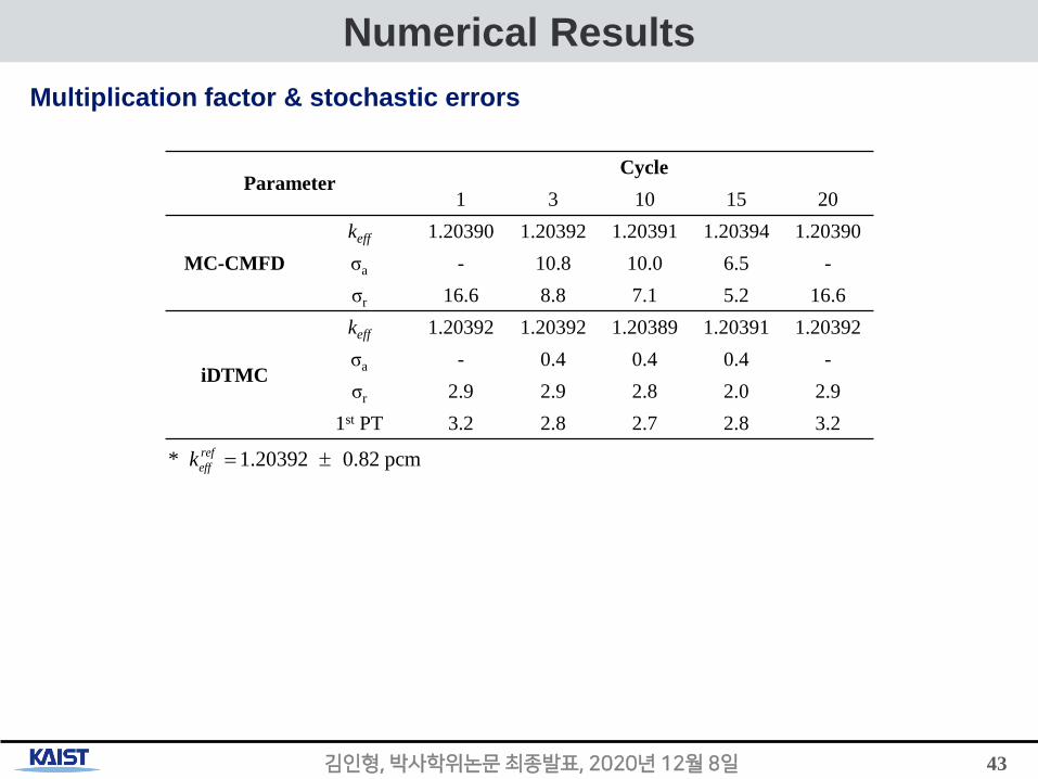
Numerical Results
Multiplication factor & stochastic errors
43김인형, 박사학위논문최종발표, 2020년 12월 8일
ParameterCycle
1 3 10 15 20
MC-CMFD
keff 1.20390 1.20392 1.20391 1.20394 1.20390
σa - 10.8 10.0 6.5 -
σr 16.6 8.8 7.1 5.2 16.6
iDTMC
keff 1.20392 1.20392 1.20389 1.20391 1.20392
σa - 0.4 0.4 0.4 -
σr 2.9 2.9 2.8 2.0 2.9
1st PT 3.2 2.8 2.7 2.8 3.2
* 1.20392 0.82 pcmref
effk

Numerical Results
Real standard deviation of the multiplication factor
44김인형, 박사학위논문최종발표, 2020년 12월 8일
0
2
4
6
8
10
12
14
16
18
0 2 4 6 8 10
Rea
l sta
nd
ard
dev
iati
on
(p
cm)
Cycles
MC-CMFD
iDTMC
1st PT (correlated)
5.6 times
3.6 times
Much more reliable solutions are obtained with the iDTMC method compared to the CMFD
Consistent results are shown in the different types of the problem

Numerical Results
Real standard deviation of the 2D pin power
– At cycle 1
45김인형, 박사학위논문최종발표, 2020년 12월 8일
MC-CMFD iDTMC
2
, , ,
1( )
bNb
i j i j i j
bb
p pN
where : batch number, : No. of batchesbb N
Cycle 1 MC-CMFD iDTMC
Avg. 0.037 0.0048
(44)

Numerical Results
Real standard deviation of the 2D pin power
– At cycle 10
46김인형, 박사학위논문최종발표, 2020년 12월 8일
MC-CMFD iDTMC
2
, , ,
1( )
bNb
i j i j i j
bb
p pN
where : batch number, : No. of batchesbb N
Cycle 10 MC-CMFD iDTMC
Avg. 0.013 0.005
(45)

Numerical Results
Relative error distribution for the 2D pin power
– At cycle 1
47김인형, 박사학위논문최종발표, 2020년 12월 8일
MC-CMFD iDTMC
*
, ,
, *
,
100 (%) i j i j
i j
i j
p p
p
* where : reference pin powerp
Error (%) MC-CMFD iDTMC
Avg. 2.3 0.42
Max. 22.3 3.8
(46)
(%)

Numerical Results
Relative error distribution for the 2D pin power
– At cycle 10
48김인형, 박사학위논문최종발표, 2020년 12월 8일
MC-CMFD iDTMC
*
, ,
, *
,
100 (%) i j i j
i j
i j
p p
p
* where : reference pin powerp
Error (%) MC-CMFD iDTMC
Avg. 0.8 0.4
Max. 7.5 3.5
(47)
(%)

Numerical Results
Computing time
– MC calculation
49김인형, 박사학위논문최종발표, 2020년 12월 8일
Standard MC MC-CMFD iDTMC
No. of inactive cycles 160 24.4 25.5
No. of active cycles 10 10 10
Inactive time (hr.) 14.0 2.4 2.4
Active time (hr.) 0.9 0.9 1.0
Total time (hr.) 15.0 3.3 3.4

Numerical Results
FOM for the multiplication factor
50김인형, 박사학위논문최종발표, 2020년 12월 8일
0
5
10
15
20
25
30
35
0.0E+0
2.0E+4
4.0E+4
6.0E+4
8.0E+4
1.0E+5
1.2E+5
1.4E+5
1.6E+5
1.8E+5
1 2 3 4 5 6 7 8 9 10
FOM
rat
io (
iDTM
C/M
C-C
MFD
)
FOM
Active cycle
MC-CMFDiDTMCFOM ratio
Much higher numerical performance is achieved
with the iDTMC method over 5 to 30 times higher

Conclusions
Conclusions
– The iDTMC method has been developed for efficient neutornic reactor analysis
• Potential bias and numerical instability disappear.
• The convergence of the FSD is accelerated and thus the computing time is reduced.
• The stochastic uncertainty is decreased even from the beginning of the active cycle.
• The stochastic error can be reasonably measured by parameter sampling scheme.
• The numerical performance is enhanced by the comparison of the conventional CMFD-assisted MC
method.
Future work
– Various applications
• Burn up calculation
• Multi-physics calculation
• Fast reactor analysis
51ANS Winter Meeting, Online, November 16-19, 2020

Thank you for your attention