An Improved Data Stream Summary

7/23/2019 An Improved Data Stream Summary

http://slidepdf.com/reader/full/an-improved-data-stream-summary 1/18

An Improved Data Stream Summary:

The Count-Min Sketch and its Applications

Graham Cormode a,∗, , S. Muthukrishnan b,1

aCenter for Discrete Mathematics and Computer Science (DIMACS), Rutgers University,

Piscataway NJ.

b Division of Computer and Information Systems, Rutgers University and AT&T Research.

Abstract

We introduce a new sublinear space data structure—the Count-Min Sketch— for summa-

rizing data streams. Our sketch allows fundamental queries in data stream summarization

such as point, range, and inner product queries to be approximately answered very quickly;

in addition, it can be applied to solve several important problems in data streams such asfinding quantiles, frequent items, etc. The time and space bounds we show for using the CM

sketch to solve these problems significantly improve those previously known — typically

from 1/ε2 to 1/ε in factor.

1 Introduction

We consider a vector a, which is presented in an implicit, incremental fashion. This vector has di-

mension n, and its current state at time t is a(t) = [a1(t), . . . ai(t), . . . , an(t)]. Initially, a is the

zero vector, ai(0) = 0 for all i. Updates to individual entries of the vector are presented as a stream

of pairs. The tth update is (it, ct), meaning that ait(t) = ait(t − 1) + ct, and ai(t) = ai(t − 1) for

all i = it. At any time t, a query calls for computing certain functions of interest on a(t).

This setup is the data stream scenario that has emerged recently. Algorithms for computing func-

tions within the data stream context need to satisfy the following desiderata. First, the space used

by the algorithm should be small, at most poly-logarithmic in n, the space required to represent a

Supported by NSF ITR 0220280 and NSF EIA 02-05116.∗ Corresponding Author

Email addresses: [email protected] (Graham Cormode),

[email protected] (S. Muthukrishnan).1 Supported by NSF CCR 0087022, NSF ITR 0220280 and NSF EIA 02-05116.

Preprint submitted to Elsevier Science 16 December 2003



explicitly. Since the space is sublinear in data and input size, the data structures used by the algo-

rithms to represent the input data stream is merely a summary—aka a sketch or synopsis [17])—of

it; because of this compression, almost no function that one needs to compute ona can be done pre-

cisely, so some approximation is provably needed. Second, processing an update should be fast and

simple; likewise, answering queries of a given type should be fast and have usable accuracy guar-

antees. Typically, accuracy guarantees will be made in terms of a pair of user specifi ed parameters,

ε and δ , meaning that the error in answering a query is within a factor of ε with probability δ . The

space and update time will consequently depend on ε and δ ; our goal will be limit this dependence

as much as is possible.

Many applications that deal with massive data, such as Internet traffi c analysis and monitoring con-

tents of massive databases, motivate this one-pass data stream setup. There has been a frenzy of ac-

tivity recently in the Algorithm, Database and Networking communities on such data stream prob-

lems, with multiple surveys, tutorials, workshops and research papers. See [12,3,28] for detailed

description of the motivations driving this area.

In recent years, several different sketches have been proposed in the data stream context that al-

low a number of simple aggregation functions to be approximated. Quantities for which effi cient

sketches have been designed include the L1 and L2 norms of vectors [2,14,23], the number of

distinct items in a sequence (ie number of non-zero entries in a(t)) [15,18,6], join and self-joinsizes of relations (representable as inner-products of vectors a(t), b(t)) [2,1], item and range sum

queries [20,5]. These sketches are of interest not simply because they can be used to directly ap-

proximate quantities of interest, but also because they have been used considerably as “black box”

devices in order to compute more sophisticated aggregates and complex quantities: quantiles [21],

wavelets [20], histograms [29,19], database aggregates and multi-way join sizes [10], etc. Sketches

thus far designed are typically linear functions of their input, and can be represented as projections

of an underlying vector representing the data with certain randomly chosen projection matrices.

This means that it is easy to compute certain functions on data that is distributed over sites, by cast-

ing them as computations on their sketches. So, they are suited for distributed applications too.

While sketches have proved powerful, they have the following drawbacks.

• Although sketches use small space, the space used typically has a Ω(1/ε2) multiplicative factor.

This is discouraging because ε = 0.1 or 0.01 is quite reasonable and already, this factor proves

expensive in space, and consequently, often, in per-update processing and function computation

times as well.

• Many sketch constructions require time linear in the size of the sketch to process each update to

the underlying data [2,21]. Sketches are typically a few kilobytes up to a megabyte or so, and

processing this much data for every update severely limits the update speed.

• Sketches are typically constructed using hash functions with strong independence guarantees,

such as p-wise independence [2], which can be complicated to evaluate, particularly for a hard-

ware implementation. One of the fundamental questions is to what extent such sophisticated in-

dependence properties are needed.

• Many sketches described in the literature are good for one single, pre-specifi ed aggregate compu-

tation. Given that in data stream applications one typically monitors multiple aggregates on the

2



same stream, this calls for using many different types of sketches, which is a prohibitive over-

head.

• Known analyses of sketches hide large multiplicative constants inside big-Oh notation.

Given that the area of data streams is being motivated by extremely high performance monitoring

applications—eg., see [12] for response time requirements for data stream algorithms that monitor

IP packet streams—these drawbacks ultimately limit the use of many known data stream algorithms

within suitable applications.

We will address all these issues by proposing a new sketch construction, which we call the Count- Min, or CM, sketch. This sketch has the advantages that: (1) space used is proportional to 1/ε; (2)

the update time is signifi cantly sublinear in the size of the sketch; (3) it requires only pairwise inde-

pendent hash functions that are simple to construct; (4) this sketch can be used for several different

queries and multiple applications; and (5) all the constants are made explicit and are small. Thus, for

the applications we discuss, our constructions strictly improve the space bounds of previous results

from 1/ε2 to 1/ε and the time bounds from 1/ε2 to 1, which is signifi cant.

Recently, a Ω(1/ε2) space lower bound was shown for a number of data stream problems: approxi-

mating frequency moments F k(t) =

k(ai(t))k, estimating the number of distinct items, and com-

puting the Hamming distance between two strings [30]. 2 It is an interesting contrast that for a

number of similar seeming problems (fi nding Heavy Hitters and Quantiles in the most general data

stream model) we are able to give an O( 1ε

) upper bound. Conceptually, CM Sketch also represents

progress since it shows that pairwise independent hash functions suffi ce for many of the fundamen-

tal data stream applications. From a technical point of view, CM Sketch and its analyses are quite

simple. We believe that this approach moves some of the fundamental data stream algorithms from

the theoretical realm to the practical.

Our results have some technical nuances:

• The accuracy estimates for individual queries depend on the L1 norm of a(t) in contrast to the

previous works that depend on the L2 norm. This is a consequence of working with simple counts.The resulting estimates are often not as tight on individual queries since L2 norm is never greater

than the L1 norm. But nevertheless, our estimates for individual queries suffi ce to give improved

bounds for the applications here where it is desired to state results in terms of L1.

• Most prior sketch constructions relied on embedding into small dimensions to estimate norms.

For example, [2] relies on embedding inspired by the Johnson-Lindenstrauss lemma [24] for es-

timating L2 norms. But accurate estimation of the L2 norm of a stream requires Ω( 1ε2 ) space [30].

Currently, all data stream algorithms that rely on such methods that estimate L p norms use Ω(1/ε2)space. One of the observations that underlie our work is while embedding into small space is

needed for small space algorithms, it is not necessary that the methods accurately estimate L2 or

in fact any L p norm, for most queries and applications in data streams. Our CM Sketch does not

help estimate L2 norm of the input, however, it accurately estimates the queries that are needed,

2 This bound has virtually been met for Distinct Items by results in [4], where clever use of hashing improves

previous bounds of O( log nε2

log 1δ ) to O(( 1

ε2 + log n)log 1

δ ).

3



which suffi ces for our data stream applications.

• Most data stream algorithm analyses thus far have followed the outline from [2] where one uses

Chebyshev and Chernoff bounds in succession to boost probability of success as well as the ac-

curacy. This process contributes to the complexity bounds. Our analysis is simpler, relying only

on the Markov inequality. Perhaps surprisingly, in this way we get tighter, cleaner bounds.

The remainder of this paper is as follows: in Section 2 we discuss the queries of our interest. We

describe our Count-Min sketch construction and how it answers queries of interest in Sections 3

and 4 respectively, and apply it to a number of problems to improve the best known complexity in

Section 5. In each case, we state our bounds and directly compare it with the best known previousresults.

All previously known sketches have many similarities. Our CM Sketch lies in the same framework,

and fi nds inspiration from these previous sketches. Section 6 compares our results to past work, and

shows how all relevant sketches can be compared in terms of a small number of parameters. This

should prove useful to readers in contrasting the vast number of results that have emerged recently

in this area. Conclusions are in Section 7.

2 Preliminaries

We consider a vector a, which is presented in an implicit, incremental fashion. This vector has di-

mension n, and its current state at time t is a(t) = [a1(t), . . . ai(t), . . . an(t)]. For convenience, we

shall usually drop t and refer only to the current state of the vector. Initially, a is the zero vector, 0,

so ai(0) is 0 for all i. Updates to individual entries of the vector are presented as a stream of pairs.

The tth update is (it, ct), meaning that

ait(t) = ait(t − 1) + ct

ai(t) = ai(t − 1) i = it

In some cases, cts will be strictly positive, meaning that entries only increase; in other cases, cts are

allowed to be negative also. The former is known as the cash register case and the latter the turnstile

case [28]. There are two important variations of the turnstile case to consider: whether a is may

become negative, or whether the application generating the updates guarantees that this will never

be the case. We refer to the fi rst of these as the general case, and the second as the non-negative case.

Many applications that use sketches to compute queries of interest—such as monitoring database

contents, analyzing IP traffi c seen in a network link—guarantee that counts will never be negative.

However, the general case occurs in important scenarios too, for example in distributed settings

where one considers the subtraction of one vector from another, say.

At any time t, a query calls for computing certain functions of interest on a(t). We focus on ap-

proximating answers to three types of query based on vectors a and b.

• A point query, denoted Q(i), is to return an approximation of ai.

4



• A range query Q(l, r) is to return an approximation of r

i=l ai.

• An inner product query, denoted Q(a, b) is to approximate a b = n

i=1 aibi.

These queries are related: a range query is a sum of point queries; both point and range queries are

specifi c inner product queries. However, in terms of approximations to these queries, results will

vary. These are the queries that are fundamental to many applications in data stream algorithms,

and have been extensively studied. In addition, they are of interest in non-data stream context. For

example, in databases, the point and range queries are of interest in summarizing the data distribu-

tion approximately; and inner-product queries allow approximation of join size of relations. Fuller

discussion of these aspects can be found in [16,28].

We will also study use of these queries to compute more complex functions on data streams. As

examples, we will focus on the two following problems. Recall that ||a||1 = n

i=1 |ai(t)|; more

generally, ||a|| p = (n

i=1 |ai(t)| p)1/p.

• (φ-Quantiles) The φ-quantiles of the cardinality ||a||1 multiset of (integer) values each in the

range 1 . . . n consist of those items with rank kφ||a||1 for k = 0 . . . 1/φ after sorting the values.

Approximation comes by accepting any integer that is between the item with rank (kφ − ε)||a||1and the one with rank (kφ + ε)||a||1 for some specifi ed ε < φ.

• ( Heavy Hitters) The φ-heavy hitters of a multiset of ||a||1 (integer) values each in the range1 . . . n, consist of those items whose multiplicity exceeds the fraction φ of the total cardinality,

i.e., ai ≥ φ||a||1. There can be between 0 and 1φ

heavy hitters in any given sequence of items.

Approximation comes by accepting any i such that ai ≥ (φ − )||a||1 for some specifi ed ε < φ.

We will assume the RAM model, where each machine word can store integers up to max||a||1, n.

Standard word operations take constant time and so we count space in terms of number of words and

we count time in terms of the number of word operations. So, if one estimates our space and time

bounds in terms of number of bits instead, a multiplicative factor log max||a||1, n is needed. Our

goal is to solve the queries and the problems above using a sketch data structure, that is using space

and time signifi cantly sublinear—polylogarithmic—in input size n and ||a|| 1. All our algorithms

will be approximate and probabilistic; they need two parameters, ε and δ , meaning that the error in

answering a query is within a factor of ε with probability δ . Both these parameters will affect the

space and time needed by our solutions. Each of these queries and problems has a rich history of

work in the data stream area. We refer the readers to surveys [28,3], tutorials [16], as well as the

general literature.

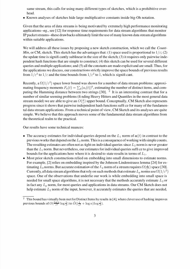
3 Count-Min Sketches

We now introduce our data structure, the Count-Min, or CM, sketch. It is named after the two basic

operations used to answer point queries, counting fi rst and computing the minimum next. We use eto denote the base of the natural logarithm function, ln.

5



1h

i t+c

+c

+c

hd

+c

t

t

t

t

Fig. 1. Each item i is mapped to one cell in each row of the array of counts: when an update of c t to item itarrives, ct is added to each of these cells

Data Structure. A Count-Min (CM) sketch with parameters (ε, δ ) is represented by a two-dimensionalarray counts with width w and depth d: count[1, 1] ...count[d, w]. Given parameters (ε, δ ), set

w = eε

and d = ln 1δ

. Each entry of the array is initially zero. Additionally, d hash functions

h1 . . . hd : 1 . . . n → 1 . . . w

are chosen uniformly at random from a pairwise-independent family.

Update Procedure. When an update (it, ct) arrives, meaning that item ait is updated by a quantity

of ct

, then ct

is added to one count in each row; the counter is determined by h j

. Formally, set∀1 ≤ j ≤ d

count[ j, h j(it)] ← count[ j, h j(it)] + ct

This procedure is illustrated in Figure 1.

The space used by Count-Min sketches is the array of wd counts, which takes wd words, and d hash

functions, each of which can be stored using 2 words when using the pairwise functions described

in [27].

4 Approximate Query Answering Using CM Sketches

For each of the three queries introduced in Section 2: Point, Range, and Inner Product queries, we

show how they can be answered using Count-Min sketches.

4.1 Point Query

We fi rst show the analysis for point queries for the non-negative case.

Estimation Procedure. The answer to Q(i) is given by ai = min j count[ j, h j(i)].

6



Theorem 1 The estimate ai has the following guarantees: ai ≤ ai; and, with probability at least

1 − δ ,ai ≤ ai + ε||a||1.

PROOF. We introduce indicator variables I i,j,k, which are 1 if (i = k) ∧ (h j(i) = h j(k)), and 0

otherwise. By pairwise independence of the hash functions, then

E(I i,j,k) = Pr[h j(i) = h j(k)] ≤ 1/ range(h j) = ε

e

.

Defi ne the variable X i,j (random over the choices of hi) to be X i,j = n

k=1 I i,j,k ak. Since all ai

are non-negative in this case, X i,j is a non-negative variable. By construction, count[ j, h j(i)] =ai + X i,j . So, clearly, min count[ j, h j(i)] ≥ ai. For the other direction, observe that

E(X i,j) = E

nk=1

I i,j,kak

≤

nk=1

akE(I i,j,k) ≤ ε

e||a||1

by pairwise independence of h j , and linearity of expectation. By the Markov inequality,

Pr

[ai > ai + ε||a||1] = Pr

[∀ j. count[ j, h j(i)] > ai + ε||a||1]= Pr[∀ j. ai + X i,j > ai + ε||a||1]

= Pr[∀ j. X i,j > eE(X i,j)] < e−d ≤ δ

The time to produce the estimate is O(ln 1δ

) since fi nding the minimum count can be done in linear

time; the same time bound holds for updates. The constant e is used here to minimize the space

used: more generally, we can set w = /b and d = logb1δ

for any b > 1 to get the same accuracy

guarantee. Choosing b = e minimizes the space used, since this solves d(wd)

db = 0, giving a cost

of (2 + eε

) ln 1δ

words. For implementations, it may be preferable to use other (integer) values of

b for simpler computations or faster updates. Note that for values of a i that are large relative to||a||1, the bound in terms of ε||a||1 can be translated into a relative error in terms of ai. This has

implications for certain applications which rely on retrieving large values, such as large wavelet or

Fourier co-effi cients.

The best known previous result using sketches was in [5]: there sketches were used to approximate

point queries. Results were stated in terms of the frequencies of individual items. For arbitrary dis-

tributions, the space used is O( 1ε2 log 1δ ), and the dependency on ε is 1

ε2 in every case considered.

A signifi cant difference between CM sketches and previous work comes in the analysis:

• All prior analyses of sketch structures compute the variance of their estimators in order to ap-

ply the Chebyshev inequality, which brings the dependency on ε2. Directly applying the Markov

inequality yields a more direct analysis which depends only on ε. Practitioners may have discov-

ered that less than O( 12 ) space is needed in practice: here, we give proof of why this is so and

the tighter bound.

7



• Because only positive quantities are added to the counters then it is possible to take the minimum

instead of the median for the estimate. This allows a simple calculation of the failure probability,

without recourse to Chernoff bounds. This signifi cantly improves the constants involved: in [5]

for example, the constant factors within the big-Oh notation is at least 256; here, the constant

factor is less than 3.

• The error bound here is one-sided, as opposed to all previous constructions which gave two-sided

errors. This brings benefi ts for many applications which use sketches.

In Section 6 we show how all existing sketch constructions can be viewed as variations of a common

procedure. This emphasizes the importance of our attempt to fi nd the simplest sketch construction

which has the best guarantees and smallest constants. A similar result holds when entries of the

implicit vector a may be negative, which is the general case.

Estimation Procedure. This time Q(i) is answered with ai = median j count[ j, h j(i)].

Theorem 2 With probability 1 − δ 1/4 ,

ai − 3ε||a||1 ≤ ai ≤ ai + 3ε||a||1.

PROOF. Observe that E(|count[ j, h j(i)] − ai|) ≤ εe

||a||1, and so the probability that any count is

off by more than 3ε||a||1 is less than 18

. Applying Chernoff bounds tells us that the probability of

the median of ln 1δ copies of this procedure being wrong is less than δ 1/4.

The time to produce the estimate is O(ln 1δ ) and the space used is (2 + e

ε) ln 1δ words. The best prior

result for this problem was the method of [5]. Again, the dependence on ε here is improved from

1/ε2 to 1/ε. By avoiding analyzing the variance of the estimator, again the analysis is simplifi ed,

and the constants are signifi cantly smaller than in previous works.

4.2 Inner Product Query

Estimation Procedure. Set ( a b) j = w

k=1 counta[ j, k]∗countb[ j, k]. Our estimation of Q(a, b)

for non-negative vectors a and b is a b = min j( a b) j .

Theorem 3 a b ≤

a b and, with probability 1 − δ ,

a b ≤ a b + ε||a||1||b||1.

PROOF.( a b) j =

ni=1

aibi +

p=q,hj( p)=hj(q)

a pbq

8



Clearly, a b ≤ a b j for non-negative vectors. By pairwise independence of h,

E( a b j − a b) = p=q

Pr[h j( p) = h j(q )]a pbq ≤ p=q

εa pbqe

≤ ε||a||1||b||1

e

So, by the Markov inequality, Pr[ a b − a b > ε||a||1||b||1] ≤ δ , as required.

The space and time to produce the estimate is O( 1ε log 1

δ). Updates are performed in time O(log 1

δ).

Note that in the special case where bi = 1, and b is zero at all other locations, then this procedure

is identical to the above procedure for point estimation, and gives the same error guarantee (since

||b||1 = 1). A similar result holds in the general case, where vectors may have negative entries.

Taking the median of ( a b) j would give a guaranteed good quality approximation; however, we

do not know of any application which makes use of inner products of such vectors, so we do not

give the full details here. We next consider the application of inner-product computation to Join size

estimation, where the vectors generated have non-negative entries.

Join size estimation is important in database query planners in order to determine the best order

in which to evaluate queries. The join size of two database relations on a particular attribute is the

number of items in the cartesian product of the two relations which agree the value of that attribute.We assume without loss of generality that attribute values in the relation are integers in the range

1 . . . n. We represent the relations being joined as vectors a and b so that the values ai represents

the number of tuples which have value i in the fi rst relation, and bi similarly for the second relation.

Then clearly ab is the join size of the two relations. Using sketches allows estimates to be made in

the presence of items being inserted to and deleted from relations. The following corollary follows

from the above theorem.

Corollary 1 The Join size of two relations on a particular attribute can be approximated up to

ε||a||1||b||1 with probability 1 − δ , by keeping space O( 1ε log 1

δ).

Previous results have used the “tug-of-war” sketches [1]. However, here some care is needed in the

comparison of the two methods: the prior work gives guarantees in terms of the L2 norm of the un-

derlying vectors, with additive error of ε||a||2||b||2; here, the result is in terms of the L1 norm. In

some cases, the L2 norm can be quadratically smaller than the L1 norm. However, when the dis-

tribution of items is non-uniform, for example when certain items contribute a large amount to the

join size, then the two norms are closer, and the guarantees of the CM sketch method is closer to the

existing method. As before, the space cost of previous methods was Ω( 1ε2 ), so there is a signifi cant

space saving to be had with CM sketches.

4.3 Range Query

Defi ne χ(l, r) to be the vector of dimension n such that χ(l, r)i = 1 ⇐⇒ l ≤ i ≤ r, and 0otherwise. Then Q(l, r) can straightforwardly be re-posed as Q(a,χ(l, r)). However, this method

9



has two drawbacks: fi rst, the error guarantee is in terms of ||a||1||χ(l, r)||1 and therefore large range

sums have an error guarantee which increases linearly with the length of the range; and second, the

time cost to directly compute the sketch for χ(l, r) depends linearly in the length of the range, r −l.

In fact, it is clear that computing range sums in this way using our sketches is not much different to

simply computing point queries for each item in the range, and summing the estimates. One way to

avoid the time complexity is to use range-sum random variables from [20] to quickly determine a

sketch of χ(l, r), but that is expensive and still does not overcome the fi rst drawback. Instead, we

adopt the use of dyadic ranges from [21]: a dyadic range is a range of the form [x2y+1 . . . (x+1)2y]for parameters x and y.

Estimation Procedure. Keep log2 n CM sketches, in order to answer range queries Q(l, r) ap-

proximately. Any range query can be reduced to at most 2log2 n dyadic range queries, which in

turn can each be reduced to a single point query. Each point in the range [1 . . . n] is a member of

log2 n dyadic ranges, one for each y in the range 0 . . . log2(n) − 1. A sketch is kept for each set of

dyadic ranges of length 2y, and update each of these for every update that arrives. Then, given a

range query Q(l, r), compute the at most 2 log2 n dyadic ranges which canonically cover the range,

and pose that many point queries to the sketches, returning the sum of the queries as the estimate.

Example 1 For n = 256 , the range [48, 107] is canonically covered by the non-overlapping dyadicranges [48 . . . 48], [49 . . . 64], [65 . . . 96], [97 . . . 104], [105 . . . 106], [107 . . . 107].

Let a[l, r] = r

i=l ai be the answer to the query Q(l, r) and let a[l, r] be the estimate using the

procedure above.

Theorem 4 a[l, r] ≤ a[l, r] and with probability at least 1 − δ ,

a[l, r] ≤ a[l, r] + 2ε log n||a||1.

PROOF. Applying the inequality of Theorem 1, then a[l, r] ≤ a[l, r]. Consider each estimator usedto form a[l, r]; the expectation of the additive error for any of these is 2 log n εe

||a||1, by linearity of

expectation of the errors of each point estimate. Applying the same Markov inequality argument as

before, the probability that this additive error is more than 2ε log n||a||1 for any estimator is less

than 1e ; hence, for all of them the probability is at most δ .

The timeto compute the estimateor to make an update is O(log(n)log 1δ

). The space used is O( log(n)ε

log 1δ

).

The above theorem states the bound for the standard CM sketch size. The guarantee will be more

useful when stated without terms of log n in the approximation bound. This can be changed by in-

creasing the size of the sketch, which is equivalent to rescaling ε. In particular, if we want to esti-mate a range sum correct up to ε||a||1 with probability 1 − δ then set ε = ε

2logn. The space used

is O( log2(n)ε

log 1δ ). An obvious improvement of this technique in practice is to keep exact counts

for the fi rst few levels of the hierarchy, where there are only a small number of dyadic ranges. This

10



improves the space, time and accuracy of the algorithm in practice, although the asymptotic bounds

are unaffected.

For smaller ranges, ranges that are powers of 2, or more generally, any range whose size can be

expressed in binary using a small number of 1s, then improved bounds are possible; we have given

the worst case bounds above.

One way to compute approximate range sums is via approximate quantiles: use an algorithm such

as [25,22] to fi nd the quantiles of the stream, and then count how many quantiles fall within the

range of interest to give an O(ε) approximation of the range query. Such an approach has severaldisadvantages: (1) Existing approximate quantile methods work in the cash register model, rather

than the more general turnstile model that our solutions work in. (2) The time cost to update the

data structure can be high, sometimes linear in the size size of the structure. (3) Existing algorithms

assume single items arriving one by one, so they do not handle fractional values or large values

being added, which can be easily handled by sketch-based approaches. (4) The worst case space

bound depends on O( 1ε log ||a||1

ε ), which can grow indefi nitely. The sketch based solution works in

fi xed space that is independent of ||a||1.

The best previous bounds for this problem in the turnstile model are given in [21], where range

queries are answered by keeping O(log n) sketches, each of size O( 1

ε2

log(n)log log n

δ ) to give ap-

proximationswith additive error ε||a||1 with probability 1−δ . Thus the space used there is O( log2 nε2

log log nδ

and the time for updates is linear in the space used. The CM sketch improves the space and time

bounds; it improves the constant factors as well as the asymptotic behavior. The time to process an

update is signifi cantly improved, since only a few entries in the sketch are modifi ed, rather than a

linear number.

5 Applications of Count-Min Sketches

By using CM sketches, we show how to improve best known time and space bounds for the two

problems from Section 2.

5.1 Quantiles in the Turnstile Model

In [21] the authors showed that fi nding the approximate φ-quantiles of the data subject to insertions

and deletions can be reduced to the problem of computing range sums. Put simply, the algorithm

is to do binary searches for ranges 1 . . . r whose range sum a[1, r] is kφ||a||1 for 1 ≤ k ≤ 1φ

− 1.

The method of [21] uses Random Subset Sums to compute range sums. By replacing this structure

with Count-Min sketches, the improved results follow immediately. By keeping log n sketches, one

for each dyadic range and setting the accuracy parameter for each to be ε/ log n and the probability

guarantee to δφ/ log(n), the overall probability guarantee for all 1/φ quantiles is achieved.

11



Theorem 5 ε-approximate φ-quantiles can be found with probability at least 1 − δ by keeping a

data structure with space O(1ε log2(n) log( logn

φδ )). The time for each insert or delete operation is

O(log(n)log( log nφδ )) , and the time to find each quantile on demand is O(log(n) log( log n

φδ )).

Choosing CM sketches over Random Subset Sums improves both the query time and the update

time from O( 1ε2

log2(n)log log nεδ

), by a factor of more than 34ε2

log n. The space requirements are also

improved by a factor of at least 34ε

.

It is illustrative to contrast our bounds with those for the problem in the weaker Cash Register

Model where items are only inserted (recall that in our stronger Turnstile model, items are deleted as

well). The previously best known space bounds for fi nding approximate quantiles is O(1ε(log2 1ε +

log2 log 1δ )) space for a randomized sampling solution [25] and O( 1

ε log(ε||a||1)) space for a deter-

ministic solution [22]. These bounds are not completely comparable, but our result is the fi rst on the

more powerful Turnstile model to be comparable to the Cash Register model bounds in the leading

1/ε term.

5.2 Heavy Hitters

We consider this problem in both the cash register model (meaning that all updates are positive)

and the more challenging turnstile model (where updates are both positive and negative, with the

restriction that count of any item is never less than zero, i.e., ai(t) ≥ 0.).

Cash Register Case. It is possible to maintain the current value of ||a||1 throughout, since ||a(t)||1 =ti=1 ci. On receiving item (it, ct), update the sketch as before and pose point query Q(it): if esti-

mate ait is above the threshold of φ||a(t)||1, it is added to a heap. The heap is kept small by checking

that the current estimated count for the item with lowest count is above threshold; if not, it is deleted

from the heap as in [5]. At the end of the input, the heap is scanned, and all items in the heap whose

estimated count is still above φ||a||1 are output.

Theorem 6 The heavy hitters can be found from an inserts only sequence of length ||a||1 , by using

CM sketches with space O( 1ε log ||a||1

δ ) , and time O(log ||a||1

δ ) per item. Every item which occurs

with count more than φ||a||1 time is output, and with probability 1 − δ , no item whose count is less

than (φ − ε)||a||1 is output.

PROOF. This procedure relies on the fact that the threshold value increases monotonically: there-

fore, if an item did not pass the threshold in the past, it cannot do so in the future without its count

increasing. By checking the estimated value every time an items value increases, no heavy hitters

will be omitted. By the one-sided error guarantee of sketches, every heavy hitter is included in the

output, but there is some possibility of including non-heavy hitters in the output. To do this, the

parameter δ is scaled to ensure that over all ||a||1 queries posed to the sketch, the probability of

mistakenly outputting an infrequent item is bounded by 1 − δ , using the union bound.

12



We can compare our results to the best known previous work. The algorithm in [5] solves this prob-

lem using Count sketches in worst case space O( 1ε2

log ||a||1δ

), which we strictly improve here. A ran-

domized algorithm given in [26] has expected space cost O( 1ε log 1

φδ ), slightly better than our worst

case space usage. Meanwhile, a deterministic algorithm in the same paper solves the problem in

worst case space O( 1ε log ||a||1

ε ). However, for both algorithms in [26] the time cost of processing

each insertion can be high (Ω(1ε )): periodically, there are operations with cost linear in the space

used. For high speed applications, our worst case time bound may be preferable.

Turnstile Case. We adopt the solution given in [8], which describes a divide and conquer pro-

cedure to fi nd the heavy hitters. This keeps sketches for computing range sums: log n different

sketches, one for each different dyadic range. When an update (it, ct) arrives, then each of these

is updated as before. In order to fi nd all the heavy hitters, a parallel binary search is performed, de-

scending one level of the hierarchy at each step. Nodes in the hierarchy (corresponding to dyadic

ranges) whose estimated weight exceeds the threshold of (φ + ε)||a||1 are split into two ranges, and

investigated recursively. All single items found in this way whose approximated count exceeds the

threshold are output.

We instead must limit the number of items output whose true frequency is less than the fraction φ.

This is achieved by setting the probability of failure for each sketch to be

δφ

2logn . This is because,at each level there are at most 1/φ items with frequency more than φ. At most twice this number

of queries are made at each level, for all of the log n levels. By scaling δ like this and applying the

union bound ensures that, over all the queries, the total probability that any one (or more) of them

overestimated by more than a fraction ε is bounded by δ , and so the probability that every query

succeeds is 1 − δ . It follows that

Theorem 7 The algorithm uses space O( 1ε log(n)log

2log(n)

δφ

) , and time O(log(n)log

2lognδφ

)

per update. Every item with frequency at least (φ + ε)||a||1 is output, and with probability 1 − δ no

item whose frequency is less than φ||a||1 is output.

The previous best known bound appears in [8], where a non-adaptive group testing approach wasdescribed. Here, the space bounds agree asymptotically but have been improved in constant fac-

tors; a further improvement is in the nature of the guarantee: previous methods gave probabilistic

guarantees about outputting the heavy hitters. Here, there is absolute certainty that this procedure

will fi nd and output every heavy hitter, because the CM sketches never underestimate counts, and

strong guarantees are given that no non-heavy hitters will be output. This is often desirable.

In some situations in practice, it is vital that updates are as fast as possible, and here update time can

be played off against search time: ranges based on powers of two can be replaced with an arbitrary

branching factor k, which reduces the number of levels to logk n, at the expense of costlier queries

and weaker guarantees on outputting non-heavy hitters.

5.2.0.1 Hierarchical Heavy Hitters A generalization of this problem is fi nding Hierarchical

Heavy Hitters [7], which assumes that the items are leaves in a hierarchy of depth h. Here the goal

13



is to fi nd all nodes in the hierarchy which are heavy hitters, after discounting the contribution of any

descendent heavy hitter nodes. Using our CM sketch, the cost of the solution given in [7] for the

turnstile model can be improved from O( hε2 log 1δ ) space and time per update to O(h

ε log 1δ ) space

and O(h log 1δ

) time per update.

6 Comparison of Sketch Techniques

We give a common framework to summarize known sketch constructions,and compare the time and

space requirements for each of the fundamental queries—point, range and inner products—using

them.

Here is a brief summary of known sketch constructions. The fi rst sketch construction was that of

Alon, Matias and Szegedy [2], whose tug-of-war sketches are computed using 4-wise random hash

functions g j mapping items to +1, −1. The j th entry of the sketch, which is a vector of length

O( 1ε2 log 1δ ), is defi ned to be

ai∗g j(i), which is easy to maintain under updates. This structure was

applied to fi nding inner products in [1,20] where, in our notation, it was shown that it is possible to

compute inner products with additive error ±ε||a||2||b||2. In [20], the authors use these sketches to

compute large wavelet coeffi cients. In particular, they show how the structure allows point queriesto be computed up to additive error of ±ε||a||2. They also compute range sums Q(l, r): here range-

summable random variables are used to compute the sums effi ciently, but this incurs a factor of

O(log n) additional time and space to compute these. Also note that here the error guarantees are

much worse for large ranges: ε(r − l + 1)||a||1.

For point queries only, then pairwise independence suffi ces for tug-of-war sketches, as observed

by [5]. These authors additionally used a second hash set of hash functions, h j , to spread out the

effect of high frequency items in their Count Sketch. For point queries, this gives the same space

bounds, but an improved time bound to O(log 1δ

) for updating the sketch 3 . Random subset sums

were introduced in [21] in order to compute point queries and range sums. Here, 2-universal hash

functions 4 h j map items to 0, 1, and the jth entry of the sketch is maintained as ni=1 ai ∗ h j(i).

The asymptotic space and time bounds for different techniques in terms of their dependence on

epsilon are summarized in Figure 2.

All of the above sketching techniques, and the one which we propose in this paper, can all be de-

scribed in a common way. Firstly, they can all be viewed as linear projections of the vector a with

appropriately chosen random vectors, but more than this, the computation of these linear projections

is very similar between all methods. Defi ne a sketch to be a two dimensional array of dimension wby d. Let h1 . . . hd be pairwise independent hash functions mapping from 1 . . . n to 1 . . . w,

3

We observe that the same idea, of replacing the averaging of O(

1

ε2

) copies of an estimator with a 2-universal hash function distributing to O( 1ε2 ) buckets can also reduce the update time for “tug-of-war”

sketches and similar constructions to O(log 1δ ).

4 In [21] the authors use a 3-wise independent hash function onto 0, 1, chosen because it is easy to com-

pute, but pairwise suffices.

14





dates to be only positive; and (3) the analysis does not consider any limited independence needed

for the hash functions, in contrast to CM sketches, which require only pairwise independence. The

methods in [13,11] as such seems to use fully independent hash functions which is prohibitive in

principle.

7 Conclusions

We have introduced the Count-Min sketch, and shown how to estimate fundamental queries such as

point, range or inner product queries as well as solve more sophisticated problems such as quantiles

and heavy hitters. The space and/or time bounds of our solutions improve previously best known

bounds for these problems. Typically the improvement is from 1/ε2 factor to 1/ε which is signif-

icant in real applications. Our CM sketch is quite simple, and is likely to fi nd many applications,

including in hardware solutions for these problems.

We have recently applied these ideas to the problem of change detection on data streams [9], and we

also believe that it can be applied to improve the time and space bounds for constructing approxi-

mate wavelet and histogram representations of data streams [19]. Also, the CM Sketch can also be

naturally extended to solve problems on streams that describe multidimensional arrays rather than

the unidimensional array problems we have discussed so far.

Our CM sketch is not effective when one wants to compute the norms of data stream inputs. These

have applications to computing correlations between data streams and tracking the number of dis-

tinct elements in streams, both of which are of great interest. It is an open problem to design ex-

tremely simple, practical sketches such as our CM Sketch for estimating such correlations and more

complex data stream applications.

References

[1] N. Alon, P. Gibbons, Y. Matias, and M. Szegedy. Tracking join and self-join sizes in limited storage. In

Proceedings of the Eighteenth ACM Symposium on Principles of Database Systems (PODS ’99) , pages

10–20, 1999.

[2] N. Alon, Y. Matias, and M. Szegedy. The space complexity of approximating the frequency moments. In

Proceedings of the Twenty-Eighth Annual ACM Symposium on the Theory of Computing, pages 20–29,

1996. Journal version in Journal of Computer and System Sciences, 58:137–147, 1999.

[3] B. Babcock, S. Babu, M. Datar, R. Motwani, and J. Widom. Models and issues in data stream systems.In Proceedings of Symposium on Principles of Database Systems (PODS) , pages 1–16, 2002.

[4] Z. Bar-Yossef, T.S. Jayram, R. Kumar, D. Sivakumar, and L. Trevisian. Counting distinct elements in

a data stream. In Proceedings of RANDOM 2002, pages 1–10, 2002.

16



[5] M. Charikar, K. Chen, and M. Farach-Colton. Finding frequent items in data streams. In Procedings

of the International Colloquium on Automata, Languages and Programming (ICALP), pages 693–703,

2002.

[6] G. Cormode, M. Datar, P. Indyk, and S. Muthukrishnan. Comparing data streams using Hamming

norms. In Proceedings of 28th International Conference on Very Large Data Bases, pages 335–345,

2002. Journal version in IEEE Transactions on Knowledge and Data Engineering 15(3):529–541, 2003.

[7] G. Cormode, F. Korn, S. Muthukrishnan, and D. Srivastava. Finding hierarchical heavy hitters in data

streams. In International Conference on Very Large Databases, pages 464–475, 2003.

[8] G. Cormode and S. Muthukrishnan. What’s hot and what’s not: Tracking most frequent items

dynamically. In Proceedings of ACM Principles of Database Systems, pages 296–306, 2003.

[9] G. Cormode and S. Muthukrishnan. What’s new: Finding significant differences in network data

streams. In Proceedings of IEEE Infocom, 2004.

[10] A. Dobra, M. Garofalakis, J. E. Gehrke, and R. Rastogi. Processing complex aggregate queries over

data streams. In Proceedings of the 2002 ACM Sigmod International Conference on Management of

Data, pages 61–72, 2002.

[11] C. Estan and G. Varghese. New directions in traffic measurement and accounting. In Proceedings of

ACM SIGCOMM , volume 32, 4 of Computer Communication Review, pages 323–338, 2002.

[12] C. Estan and G. Varghese. Data streaming in

computer networks. In Proceedings of Workshop on Management and Processing of Data Streams ,

http://www.research.att.com/conf/mpds2003/schedule/estanV.ps , 2003.

[13] M. Fang, N. Shivakumar, H. Garcia-Molina, R. Motwani, and J. D. Ullman. Computing iceberg queries

efficiently. In Proceedings of the Twenty-fourth International Conference on Very Large Databases,

pages 299–310, 1998.

[14] J. Feigenbaum, S. Kannan, M. Strauss, and M. Viswanathan. An approximate L1-difference algorithm

for massive data streams. In Proceedings of the 40th Annual Symposium on Foundations of Computer

Science, pages 501–511, 1999.

[15] P. Flajolet and G. N. Martin. Probabilistic counting. In 24th Annual Symposium on Foundations of

Computer Science, pages 76–82, 1983. Journal version in Journal of Computer and System Sciences,

31:182–209, 1985.

[16] M. Garofalakis, J. Gehrke, and R. Rastogi. Querying and mining data streams: You only get one look.

In Proceedings of the ACM SIGMOD International Conference on Management of Data, 2002.

[17] P. Gibbons and Y. Matias. Synopsis structures for massive data sets. DIMACS Series in Discrete

Mathematics and Theoretical Computer Science, A, 1999.

[18] P. Gibbons and S. Tirthapura. Estimating simple functions on the union of data streams. In Proceedings

of the 13th ACM Symposium on Parallel Algorithms and Architectures, pages 281–290, 2001.

[19] A. Gilbert, S. Guha, P. Indyk, Y. Kotidis, S. Muthukrishnan, and M. Strauss. Fast, small-space algorithms

for approximate histogram maintenance. In Proceedings of the 34th ACM Symposium on Theory of

Computing, pages 389–398, 2002.

17



[20] A. Gilbert, Y. Kotidis, S. Muthukrishnan, and M. Strauss. Surfing wavelets on streams: One-pass

summaries for approximate aggregate queries. In Proceedings of 27th International Conference on Very

Large Data Bases, pages 79–88, 2001. Journal version in IEEE Transactions on Knowledge and Data

Engineering, 15(3):541–554, 2003.

[21] A. C. Gilbert, Y. Kotidis, S. Muthukrishnan, and M. Strauss. How to summarize the universe: Dynamic

maintenance of quantiles. In Proceedings of 28th International Conference on Very Large Data Bases ,

pages 454–465, 2002.

[22] M. Greenwald and S. Khanna. Space-efficient online computation of quantile summaries. SIGMOD

Record (ACM Special Interest Group on Management of Data), 30(2):58–66, 2001.

[23] P. Indyk. Stable distributions, pseudorandom generators, embeddings and data stream computation. In

Proceedings of the 40th Symposium on Foundations of Computer Science , pages 189–197, 2000.

[24] W.B. Johnson and J. Lindenstrauss. Extensions of Lipshitz mapping into Hilbert space. Contemporary

Mathematics, 26:189–206, 1984.

[25] G. S. Manku, S. Rajagopalan, and B. G. Lindsay. Approximate medians and other quantiles in one

pass and with limited memory. In Proceedings of the ACM SIGMOD International Conference on

Management of Data, pages 426–435, 1998.

[26] G.S. Manku and R. Motwani. Approximate frequency counts over data streams. In Proceedings of 28th

International Conference on Very Large Data Bases, pages 346–357, 2002.

[27] R. Motwani and P. Raghavan. Randomized Algorithms. Cambridge University Press, 1995.

[28] S. Muthukrishnan. Data streams: Algorithms and applications. In ACM-SIAM Symposium on Discrete

Algorithms, http://athos.rutgers.edu/∼muthu/stream-1-1.ps, 2003.

[29] N. Thaper, P. Indyk, S. Guha, and N. Koudas. Dynamic multidimensional histograms. In Proceedings

of the ACM SIGMOD International Conference on Management of Data , pages 359–366, 2002.

[30] D. Woodruff. Optimal space lower bounds for all frequency moments. In ACM-SIAM Symposium on

Discrete Algorithms, 2004.

18

Documents

An Improved Data Stream Summary