Pattern Recognition 42 (2009) 2460 -- 2469

Contents lists available at ScienceDirect

Pattern Recognition

journal homepage: www.e lsev ier .com/ locate /pr

An improved box-countingmethod for image fractal dimension estimation

Jian Lia, Qian Dub,∗, Caixin Suna

aState Key Laboratory of Power Transmission Equipment & System Security and New Technology, College of Electrical Engineering, Chongqing University, Chongqing 400044, ChinabDepartment of Electrical and Computer Engineering, Mississippi State University, MS 39762, USA

A R T I C L E I N F O A B S T R A C T

Article history:Received 6 September 2007Received in revised form 14 January 2009Accepted 2 March 2009

Keywords:Fractal dimensionBox-counting dimensionFractional Brownian motionTexture imageRemote sensing image

Fractal dimension (FD) is a useful feature for texture segmentation, shape classification, and graphicanalysis in many fields. The box-counting approach is one of the frequently used techniques to estimatethe FD of an image. This paper presents an efficient box-counting-based method for the improvement ofFD estimation accuracy. A new model is proposed to assign the smallest number of boxes to cover theentire image surface at each selected scale as required, thereby yielding more accurate estimates. The ex-periments using synthesized fractional Brownian motion images, real texture images, and remote sensingimages demonstrate this new method can outperform the well-known differential boxing-counting (DBC)method.

© 2009 Elsevier Ltd. All rights reserved.

1. Introduction

Fractal geometry provides a mathematical model for many com-plex objects found in nature [1–3], such as coastlines, mountains,and clouds. These objects are too complex to possess characteristicsizes and to be described by traditional Euclidean geometry. Self-similarity is an essential property of fractal in nature and may bequantified by a fractal dimension (FD). The FD has been applied intexture analysis and segmentation [4–6], shape measurement andclassification [7], image and graphic analysis in other fields [8,9].

There are quite a few definitions of FDs making sense in certainsituations. Thus, different methods have been proposed to estimatethe FD. Voss summarized and classified these methods into threemajor categories: the box-counting methods, the variance methods,and the spectral methods [10]. The box-counting dimension is themost frequently used for measurements in various application fields.The reason for its dominance lies in its simplicity and automatic com-putability [3]. Several practical box-counting methods were broughtforward for FD estimation [11–17]. In Ref. [12], the differential box-counting (DBC) method was compared with other four methods pro-posed by Gangepain and Roques-Carmes [11], Peleg [18], Pentland[1], and Keller [19], respectively. The DBC method was consideredas a better method, as was also supported by the investigation con-ducted in Refs. [20,21].

However, in [14] the drawbacks of the DBC method were pointedout, such as the proneness of overcounting or undercounting thenumber of boxes, and then the shifting DBC and the scanning

∗ Corresponding author.E-mail address: du@ece.msstate.edu (Q. Du).

0031-3203/$ - see front matter © 2009 Elsevier Ltd. All rights reserved.doi:10.1016/j.patcog.2009.03.001

DBC were proposed which may provide more accurate estimates.Buczkowski et al. [13] also presented a new procedure to eliminateanother two problems of a box-counting method, i.e., the boardereffect and non-integer values of selected copy scales.

According to our experience on the analysis of gray level images,the DBC method may provide unreasonable FDs of images, whichmay be less than two, particularly when these images are quitesmooth. Therefore, we develop a new method for more accurate es-timates, resulting from completely different strategies in box scaleselection, box number determination, and image intensity surfacepartition. The experimental results using the synthesized fractionalBrownian motion (fBm) images, real texture images, and remotesensing images, demonstrated its advantages.

This paper is organized as follows. In Section 2, the basic conceptof FD and procedures of the original DBC method are introduced.The problems of the DBC method are discussed in this section aswell. In Section 3, the new approaches for selecting appropriate boxscale, determining box numbers, and partitioning image intensitysurface are presented. In Section 4, fBm images, real texture images,smoothened texture images, and remote sensing images, are usedto evaluate the proposed box-counting estimation. Section 5 drawsthe conclusions.

2. Basic definition and DBC estimate

The basic principle to estimate FD is based on the concept ofself-similarity. The FD of a bounded set A in Euclidean n-space isdefined as

D = limr→0

log(Nr)log(1/r)

(1)

J. Li et al. / Pattern Recognition 42 (2009) 2460 -- 2469 2461

Image plane

Gray intensity

surface

Box 1

Box 2

Box 3

Fig. 1. Sketch of determination of the number of boxes by the DBC method.

where Nr is the least number of distinct copies of A in the scale r.The union of Nr distinct copies must cover the set A completely.

The FD can only be calculated for deterministic fractals. For anobject with deterministic self-similarity, its FD is equal to its box-counting dimension DB. However, natural scenes are not the idealand deterministic fractals. The box-counting dimension DB is an es-timate of D, calculated by using a box-counting method. The DBCmethod is introduced as follows.

Consider an image of size M×M as a three-dimensional (3-D) spa-tial surface with (x, y) denoting pixel position on the image plane,and the third coordinate (z) denoting pixel gray level. In the DBCmethod, the (x, y) plane is partitioned into non-overlapping blocksof size s×s. The scale of each block is r = s, where M/2 � s> 1 ands is an integer. Nr is counted in the DBC method using the followingprocedure. On each block there is a column of boxes of size s×s×s′,where s′ is the height of each box, G/s′ = M/s, and G is the totalnumber of gray levels. For example, s = s′ = 3 in Fig. 1 [12]. Assignnumbers 1, 2, . . . , to the boxes as shown in Fig. 1. Let the minimumand maximum gray level in the (i, j)th block fall into the kth and lthboxes, respectively. The boxes covering this block are counted in thenumber as

nr(i, j) = l − k + 1 (2)

where the subscript r denotes the result using the scale r. For exam-ple, nr(i, j) = 3−1+1 as illustrated in Fig. 1. Considering contributionsfrom all blocks, Nr is counted for different values of r as

Nr =∑i,j

nr(i, j) (3)

Then the FD can be estimated from the least squares linear fit of log(Nr) versus log (1/r).

There are three major problems in the aforementioned procedurein the original DBC method:

(1) Box height selection: When the boxes in the size s×s×s′ are as-signed to cover the image surface, the value of s is limited tothe image size but s′ may be flexible. Intuitively, a smaller mea-surement error results from a smaller measurement scale. If theheight of boxes is selected as s′ = sG/M as in the DBC method,it may have a larger value when s is increased. Then the box ina larger scale may result in greater computational error whencounting the box numbers. How to select an appropriate boxscale in height is the first problem to be resolved.

(2) Box number calculation: The DBC method assigns a column ofboxes on a block starting from the gray level zero, which inducesthe second problem illustrated in Fig. 2, where pixels A and B

Image plane

Box 1

Box 2

Box 3

Pixel A

Pixel B

Fig. 2. Two pixels fall into two boxes with the size 3×3×3 but have the distancesmaller than 3 in height direction.

represent the maximum and minimum gray levels of the block(they have the z coordinates corresponding to the gray levelvalues). If a column of boxes with the size 3×3×3 cover thisblock, the two pixels are assigned in boxes 2 and 3 in Fig. 2.However, the distance between the two pixels in the z directionis smaller than 3. Only one box can cover this block even thoughits pixels with the maximum and minimum gray levels fall intotwo different boxes, which is also the result from Eq. (2). So theDBCmethod cannot acquire the least number of boxes that coverthe block. A new approach to find the least numbers of boxescovering each block needs to be proposed.

(3) Image intensity surface partition: The pixels in a digital image arediscretized results of a continuous image with infinite resolu-tion. If the boxes are assigned as in the DBC method, there isa gap between any two spatially adjacent boxes. This indicatesthat all boxes in the DBC method cannot completely cover theentire image when the image intensity surface is considered tobe continuous. Due to this fact, there must be estimation errorsexisting in the results from the DBC method. An approach toassign boxes that can cover the full image surface needs to bedeveloped.

Due to the above three problems, the accuracy of the original DBCmethod is limited. Three modifications in our box-counting estima-tion method are proposed for improvement, which is presented inSection 3.

3. A new box-counting method

3.1. Basic concept of the new box-counting method

Let z = f(x, y) be an ideal fractal image with a 3-D continuoussurface. It is divided into distinct copies and a copy has a minimumdenoted as z1 = f(x1, y1) and a maximum denoted as z2 = f(x2, y2),when x1 � x< x2 and y1 � y< y2. Let dx and dy be the lengths ofthe copy in the directions of x and y, respectively, and dz be the heightin the direction of z. Because z = f(x, y) is continuous, we can obtaindx = x2−x1, dy = y2−y1, and dz = z2−z1. Suppose dx = dy and definethe box scale as r = dx = dy. Assume a column of boxes with the sizeof dx×dx×dx cover the copy of surface completely. The number ofthis column of boxes is equal to the integer part of (dz/r+1). UsingEq. (1), the FD of an ideal fractal can be determined via least squareslinear fit. In other words, Eq. (1) indicates that there exists definitelya scale range [r1, r2] in which the FD estimate of the ideal fractalsurface can be calculated as

D = − log Nr1 − log Nr2log r1 − log r2

(4)

2462 J. Li et al. / Pattern Recognition 42 (2009) 2460 -- 2469

where Nr1 and Nr2 are the numbers of boxes covering the ideal fractalsurface when the box scales are r1 and r2, respectively. When r1and r2 approach zero, the scale range can be found such that theFD estimate error approaches zero. Any two values of r in [r1, r2]and their corresponding Nr can be used to substitute the parametersin (4) and obtain D since Nr versus r is an exact straight line in alog–log plot in this scale range. The negative slope of the straightline is equal to D.

Due to the limited resolution, FD estimates of digital image sur-faces have discrepancy from their true FDs, even though they areideal fractals. If appropriate approaches for box number counting areemployed, errors of FD estimates could be small enough. From thepreceding description about FD calculation of an ideal and continu-ous fractal surface, the basic concepts of three modifications to beproposed for the DBC method are briefly summarized as below withmore details being presented in the following sections.

(1) Let a new scale r′ = r/c, where c is a positive real number greaterthan 1. The number of boxes covering a copy is calculated asthe integer part of (dz/r′+1). Because r′ < r and dz/r′ > dz/r, theresidual part of dz/r′ is smaller than that of dz/r. Thus, the errorsintroduced by the box scale r′ are smaller than r in the originalDBC method. This leads to the modification A in Section 3.2.

(2) dz is used to count the numbers of box covering a copy of im-age surface instead of z, the gray levels of pixels, being used forEq. (2) in the original DBS method, resulting in more accu-rate box number counting. This leads to the modification B inSection 3.3.

(3) The scale r for an ideal and continuous surface is defined asr = dx = dy, where dx = x2−x1 and dy = y2−y1. Therefore, for adigital image, if the distance between any two neighboring pixelsare 1, then the scale r = s−1 rather than r in the original DBCmethod, when s×s pixels exist in a copy of a digital image surface.This leads to the modification C in Section 3.4.

3.2. Box height selection (modification A)

Let the mean and the standard deviation of a digital image be �and �. Suppose most pixels fall into the interval of gray level within[�−a�, �+a�]. The box height r′ is selected as

r′ = r1 + 2a�

(5)

where a is a positive integer and 2a� can indicate image roughness.How to select the optimum value of a will be presented in Section4.1. As a result, a box with smaller height is chosen for an imagesurface with higher intensity variation.

Compared to the height of boxes in the DBC method, the heightof boxes in the improved DBC method is much smaller at differentbox scale of r. For example, if an image has the size of 128×128 with128 gray levels and the standard deviation � being 15, the box heightis r′ = r = 3 in the DBC method and it becomes r′ = r/91 when a = 3according to Eq. (4). So the newmethod uses finer scales to count thenumbers of boxes covering each block and the entire image surfacethrough automatic adjustment based on image smoothness.

3.3. Box number calculation (modification B)

If the maximum and minimum gray levels of the (i, j)th blockare l and k, respectively, the number of boxes that cover the blocksurface can be calculated as

nr(i, j) ={ceil

(l−kr′

), l� k

1, l = k(6)

The pixel located at the vertex

Two adjacent blocks with 4×4 pixels each

Column 1

Image plane

Gray intensitysurface

Column 2

Box 1 Box 1

Box 2 Box 2

Box 3 Box 3

Boundary pixels

Fig. 3. Box number determination by the improved DBC method.

where ceil ( · ) denotes the function to round a value to the nearestand greater integer. The physical meaning of Eq. (5) is that the boxesare assigned from the minimum gray level of the block rather thangray level 0. It is expected that nr(i, j) is the least number of boxescovering the surface of the (i, j)th block.

For the example shown in Fig. 2, r′ = 3 and the distance betweenthe two pixels A and B in height direction is smaller than 3. By usingEq. (6), the number of boxes coving the block is nr = 1, which is theexact number of boxes covering the block.

3.4. Image intensity surface partition (modification C)

To ensure that the image intensity surface is completely covered,the following partition scheme is applied:

(1) Partition an image with the size M×M into equivalent blockswith s×s pixels. Any two spatially adjacent blocks overlap at theboundary by one row (or column, i.e., s pixels). For instance, animage of size 16×13 pixels shown in Fig. 3 is partitioned into 20blocks. Each block possesses 4×4 pixels. Any two adjacent blocksoverlap by 4 pixels on their shared boundary.

(2) Let the scale r of a block with s×s pixels be s−1, which representsthe maximum distance between any two pixels in a block onthe same vertical or horizontal direction. For example, scale r ofeach block in Fig. 3 is equal to 3.

After this partition, pixels on the boundary of two neighboringblocks, falling into the (i, j)th and the (i+1, j)th grids, are taken intoaccount for computing nr(i, j) and nr(i+1, j) as well. However, thoseboundary pixels give different contributions to nr(i, j) and nr(i+1, j).If their values represent the true values of pixels in the (i, j)th block,they are used for the computation of nr(i+1, j) as approximate valuesof boundary pixels. Fortunately, their values approach the true val-ues of boundary pixels in the (i+1, j)th block since the image inten-sity surface is considered to be contiguous. Hence, an image planeis partitioned in the way that any two neighboring blocks approachzero in distance and all boxes cover the image intensity surfacecompletely. In Section 4, it will be shown that any two neighboringblocks overlapping only one row of pixels on their boundary is thebest selection for the image intensity surface partition.

3.5. Algorithm summary

The detailed algorithm of the improved DBC method can be sum-marized as follows:

(1) Divide the image into blocks of size s×s. Any two adjacent blocksoverlap by one row (and column) of pixels at the boundary.

J. Li et al. / Pattern Recognition 42 (2009) 2460 -- 2469 2463

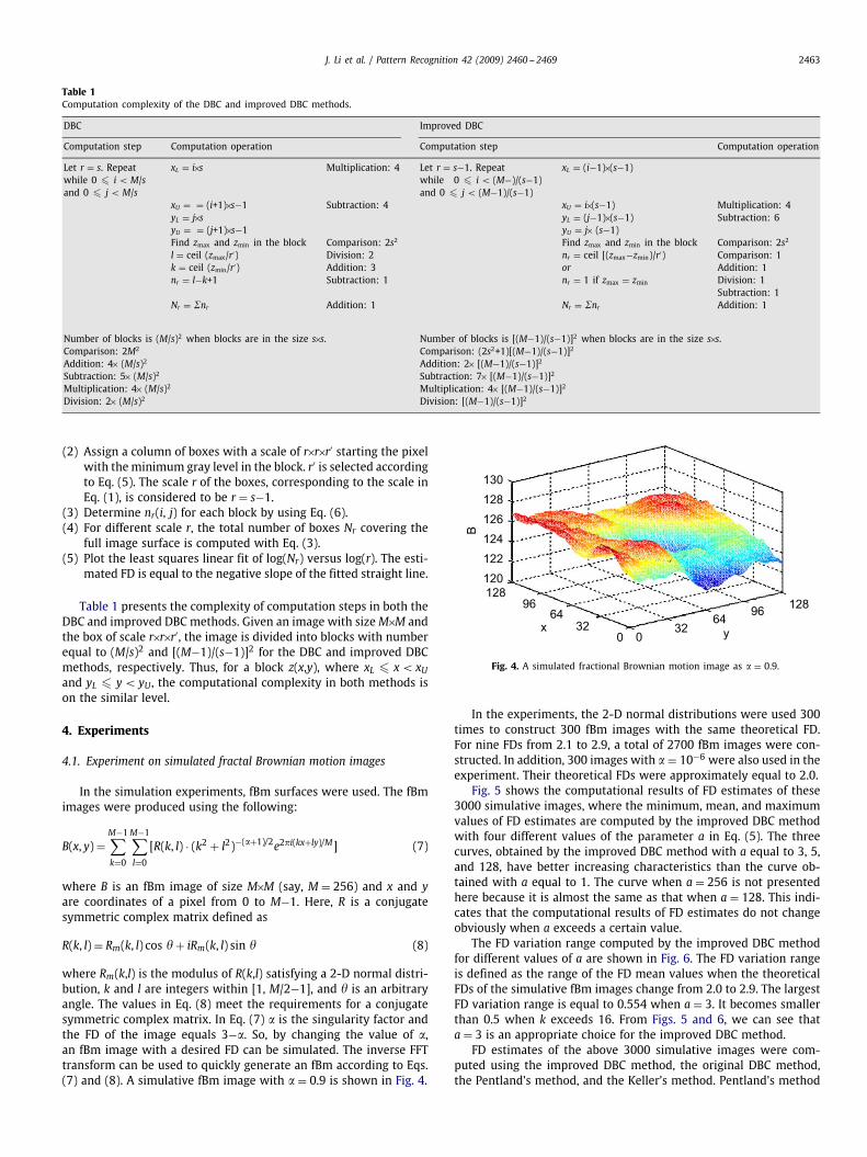
Table 1Computation complexity of the DBC and improved DBC methods.

DBC Improved DBC

Computation step Computation operation Computation step Computation operation

Let r = s. Repeatwhile 0 � i < M/sand 0 � j < M/s

xL = i×s Multiplication: 4 Let r = s−1. Repeatwhile 0 � i < (M−)/(s−1)and 0 � j < (M−1)/(s−1)

xL = (i−1)×(s−1)

xU = = (i+1)×s−1 Subtraction: 4 xU = i×(s−1) Multiplication: 4yL = j×s yL = (j−1)×(s−1) Subtraction: 6yU = = (j+1)×s−1 yU = j× (s−1)Find zmax and zmin in the block Comparison: 2s2 Find zmax and zmin in the block Comparison: 2s2

l = ceil (zmax/r′) Division: 2 nr = ceil [(zmax−zmin)/r′) Comparison: 1k = ceil (zmin/r′) Addition: 3 or Addition: 1nr = l−k+1 Subtraction: 1 nr = 1 if zmax = zmin Division: 1

Subtraction: 1Nr = �nr Addition: 1 Nr = �nr Addition: 1

Number of blocks is (M/s)2 when blocks are in the size s×s. Number of blocks is [(M−1)/(s−1)]2 when blocks are in the size s×s.Comparison: 2M2 Comparison: (2s2+1)[(M−1)/(s−1)]2

Addition: 4× (M/s)2 Addition: 2× [(M−1)/(s−1)]2

Subtraction: 5× (M/s)2 Subtraction: 7× [(M−1)/(s−1)]2

Multiplication: 4× (M/s)2 Multiplication: 4× [(M−1)/(s−1)]2

Division: 2× (M/s)2 Division: [(M−1)/(s−1)]2

(2) Assign a column of boxes with a scale of r×r×r′ starting the pixelwith the minimum gray level in the block. r′ is selected accordingto Eq. (5). The scale r of the boxes, corresponding to the scale inEq. (1), is considered to be r = s−1.

(3) Determine nr(i, j) for each block by using Eq. (6).(4) For different scale r, the total number of boxes Nr covering the

full image surface is computed with Eq. (3).(5) Plot the least squares linear fit of log(Nr) versus log(r). The esti-

mated FD is equal to the negative slope of the fitted straight line.

Table 1 presents the complexity of computation steps in both theDBC and improved DBC methods. Given an image with sizeM×M andthe box of scale r×r×r′, the image is divided into blocks with numberequal to (M/s)2 and [(M−1)/(s−1)]2 for the DBC and improved DBCmethods, respectively. Thus, for a block z(x,y), where xL � x< xUand yL � y< yU, the computational complexity in both methods ison the similar level.

4. Experiments

4.1. Experiment on simulated fractal Brownian motion images

In the simulation experiments, fBm surfaces were used. The fBmimages were produced using the following:

B(x, y) =M−1∑k=0

M−1∑l=0

[R(k, l) · (k2 + l2)−(�+1)/2e2�i(kx+ly)/M] (7)

where B is an fBm image of size M×M (say, M = 256) and x and yare coordinates of a pixel from 0 to M−1. Here, R is a conjugatesymmetric complex matrix defined as

R(k, l) = Rm(k, l) cos � + iRm(k, l) sin � (8)

where Rm(k,l) is the modulus of R(k,l) satisfying a 2-D normal distri-bution, k and l are integers within [1, M/2−1], and � is an arbitraryangle. The values in Eq. (8) meet the requirements for a conjugatesymmetric complex matrix. In Eq. (7) � is the singularity factor andthe FD of the image equals 3−�. So, by changing the value of �,an fBm image with a desired FD can be simulated. The inverse FFTtransform can be used to quickly generate an fBm according to Eqs.(7) and (8). A simulative fBm image with � = 0.9 is shown in Fig. 4.

130128126124122120128

9664

320

x0

3264 96 128

y

B

Fig. 4. A simulated fractional Brownian motion image as � = 0.9.

In the experiments, the 2-D normal distributions were used 300times to construct 300 fBm images with the same theoretical FD.For nine FDs from 2.1 to 2.9, a total of 2700 fBm images were con-structed. In addition, 300 images with � = 10−6 were also used in theexperiment. Their theoretical FDs were approximately equal to 2.0.

Fig. 5 shows the computational results of FD estimates of these3000 simulative images, where the minimum, mean, and maximumvalues of FD estimates are computed by the improved DBC methodwith four different values of the parameter a in Eq. (5). The threecurves, obtained by the improved DBC method with a equal to 3, 5,and 128, have better increasing characteristics than the curve ob-tained with a equal to 1. The curve when a = 256 is not presentedhere because it is almost the same as that when a = 128. This indi-cates that the computational results of FD estimates do not changeobviously when a exceeds a certain value.

The FD variation range computed by the improved DBC methodfor different values of a are shown in Fig. 6. The FD variation rangeis defined as the range of the FD mean values when the theoreticalFDs of the simulative fBm images change from 2.0 to 2.9. The largestFD variation range is equal to 0.554 when a = 3. It becomes smallerthan 0.5 when k exceeds 16. From Figs. 5 and 6, we can see thata = 3 is an appropriate choice for the improved DBC method.

FD estimates of the above 3000 simulative images were com-puted using the improved DBC method, the original DBC method,the Pentland's method, and the Keller's method. Pentland's method

2464 J. Li et al. / Pattern Recognition 42 (2009) 2460 -- 2469

Fig. 5. FD estimates of fBm images computed by the improved DBC method withdifferent values of a.

Fig. 6. FD variation range of fBm images computed by the improved DBC methodwith different values of a.

is a method of estimating FD by using the Fourier power spectrumof image intensity surface but not by counting the number of boxesthat cover up total image intensity surface [1]; Keller's method in-troduces probability to count box number covering up total imageintensity surface, which differs completely from the original DBC andthe improved DBC [19]. They were selected for performance com-parison due to their relatively robust performance based on our ex-perience. The Pentland's method and the Keller's method are calledbriefly as Pent and Kell hereafter, respectively. As shown in Fig. 7,the improved DBC method generates FD means changing from 2.04to 2.59, which are more accurate than that from 2.01 to 2.41 bythe original DBC method. Pent generates FD means changing almostlinearly, and Kell has wider variation range of FD means than theimproved DBC method. However, unreasonable results of computa-tional FDs smaller than 2 may be obtained by Pent and Kell, whensimulative fBm images have small theoretical FDs. Fig. 7 also showsthe improved DBC method, with two rows overlapped between twoadjacent blocks, generates computational FD equal to 2.26, which ismuch greater than 2.0 when the estimated fBm images has theoret-ical FD of 2.0. Moreover, an image with all pixels having zero graylevels was used to identify if it is proper to select two rows over-lapped in the modification C of the improved DBC. The theoretical FDof the image is equal to 2. The computational FD is 2.00 computed by

Fig. 7. Fractal dimension estimates of fBm images when their theoretical FDs increasefrom 2.0 to 2.9.

both the DBC and improved DBC. But the improved DBC generatescomputational FD of 2.14 when two rows are overlapped in modifi-cation C. More computational results for three and four overlappedrows are 2.42 and 2.87, which are obviously unreasonable.

The fit error E is used to measure the least squares linear fit ofthe log(Nr) versus log(r). The lower fit error result from the better fit.The fit error E of points (x, y) from their fitted straight line satisfyingy = cx+d is defined as

E = 1n

√√√√ n∑i=1

cxi + d − yi1 + c2

(9)

where y and x denote log(Nr) and log(r) for the above approachesbut not for Pent. They denote log(S) and log(f) for Pent, where S(f1,f2) is the power spectra density distribution of a fBm image B(x, y)and f = √

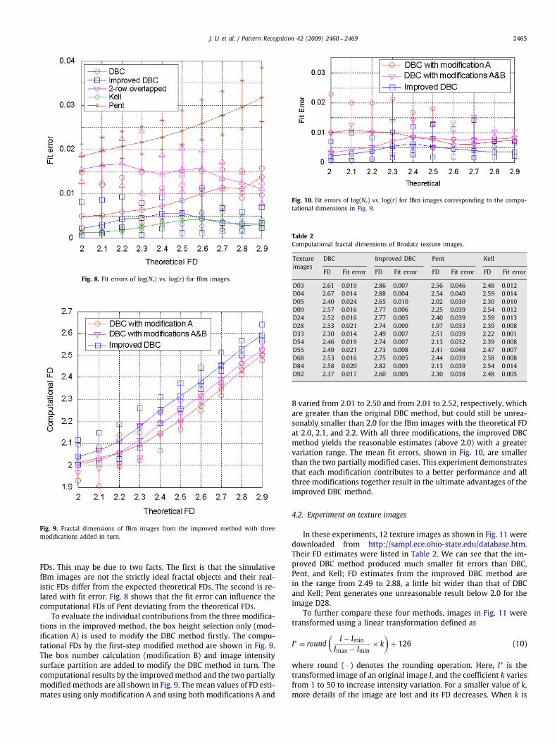
(f12+f22). Ref. [4] indicated that DBC method produced thesmall fit errors in computing FDs of texture images. Fig. 8 presentsthe minimum, mean, and maximum values of the fit errors for thesimulative fBm images. First of all, Fig. 8 shows that selection of twooverlapped rows is not appropriate for the improved DBC method,because the fit errors obtained by this way are obviously greaterthan the improved DBC method with one-overlapped row. Second,the improved DBC method has the smaller fit errors than DBC andPent. This proves once more that the improved DBC method is moreeffective than these two methods. Finally, Kell has a little bit smallerfit errors than the improved DBC. But its computation complexity ismuch greater than DBC, presented in [12], and therefore than theimproved DBC from Table 1.

It is noteworthy that the computational results of DBC, Kell, andPent include some FD estimates that are smaller than 2.0 for thefBm images when the theoretical FD equal to 2.0, 2.1, and 2.2. Theimproved DBC method always generated reasonable FD estimates,which should be above 2.0 for any images in any cases. Also, consid-ering the above analysis results of variation range of computationalFDs, fit error, and computation complexity, we obtain a conclusionthat the improved DBC method can provide more reasonable and ac-curate FD estimates for these fBm images than DBC, Kell, and Pent;meanwhile, it keeps the computational complexity as low as in DBC.It is also worth noting that the average values of estimated FDs bythe improved DBC, DBC, Kell, and Pent, deviate from the theoretical

J. Li et al. / Pattern Recognition 42 (2009) 2460 -- 2469 2465

Fig. 8. Fit errors of log(Nr) vs. log(r) for fBm images.

Fig. 9. Fractal dimensions of fBm images from the improved method with threemodifications added in turn.

FDs. This may be due to two facts. The first is that the simulativefBm images are not the strictly ideal fractal objects and their real-istic FDs differ from the expected theoretical FDs. The second is re-lated with fit error. Fig. 8 shows that the fit error can influence thecomputational FDs of Pent deviating from the theoretical FDs.

To evaluate the individual contributions from the three modifica-tions in the improved method, the box height selection only (mod-ification A) is used to modify the DBC method firstly. The compu-tational FDs by the first-step modified method are shown in Fig. 9.The box number calculation (modification B) and image intensitysurface partition are added to modify the DBC method in turn. Thecomputational results by the improved method and the two partiallymodified methods are all shown in Fig. 9. The mean values of FD esti-mates using only modification A and using both modifications A and

Fig. 10. Fit errors of log(Nr) vs. log(r) for fBm images corresponding to the compu-tational dimensions in Fig. 9.

Table 2Computational fractal dimensions of Brodatz texture images.

Textureimages

DBC Improved DBC Pent Kell

FD Fit error FD Fit error FD Fit error FD Fit error

D03 2.61 0.019 2.86 0.007 2.56 0.046 2.48 0.012D04 2.67 0.014 2.88 0.004 2.54 0.040 2.59 0.014D05 2.40 0.024 2.65 0.010 2.02 0.030 2.30 0.010D09 2.57 0.016 2.77 0.006 2.25 0.039 2.54 0.012D24 2.52 0.016 2.77 0.005 2.40 0.039 2.59 0.013D28 2.53 0.021 2.74 0.009 1.97 0.033 2.39 0.008D33 2.30 0.014 2.49 0.007 2.51 0.039 2.22 0.001D54 2.46 0.019 2.74 0.007 2.13 0.032 2.39 0.008D55 2.49 0.021 2.73 0.008 2.41 0.048 2.47 0.007D68 2.53 0.016 2.75 0.005 2.44 0.039 2.58 0.008D84 2.58 0.020 2.82 0.005 2.13 0.039 2.54 0.014D92 2.37 0.017 2.60 0.005 2.30 0.038 2.48 0.005

B varied from 2.01 to 2.50 and from 2.01 to 2.52, respectively, whichare greater than the original DBC method, but could still be unrea-sonably smaller than 2.0 for the fBm images with the theoretical FDat 2.0, 2.1, and 2.2. With all three modifications, the improved DBCmethod yields the reasonable estimates (above 2.0) with a greatervariation range. The mean fit errors, shown in Fig. 10, are smallerthan the two partially modified cases. This experiment demonstratesthat each modification contributes to a better performance and allthree modifications together result in the ultimate advantages of theimproved DBC method.

4.2. Experiment on texture images

In these experiments, 12 texture images as shown in Fig. 11 weredownloaded from http://sampl.ece.ohio-state.edu/database.htm.Their FD estimates were listed in Table 2. We can see that the im-proved DBC method produced much smaller fit errors than DBC,Pent, and Kell; FD estimates from the improved DBC method arein the range from 2.49 to 2.88, a little bit wider than that of DBCand Kell; Pent generates one unreasonable result below 2.0 for theimage D28.

To further compare these four methods, images in Fig. 11 weretransformed using a linear transformation defined as

I∗ = round(

I − Imin

Imax − Imin× k

)+ 126 (10)

where round ( · ) denotes the rounding operation. Here, I* is thetransformed image of an original image I, and the coefficient k variesfrom 1 to 50 to increase intensity variation. For a smaller value of k,more details of the image are lost and its FD decreases. When k is

2466 J. Li et al. / Pattern Recognition 42 (2009) 2460 -- 2469

D03 D04 D05 D09

D24 D28 D33 D54

D55 D68 D84 D92

Fig. 11. Brodatz texture images.

Fig. 12. Fractal dimensions of D04* transformed with different k computed by thefour methods.

large, the transformed images look similar to their original images, sotheir FDs should be close. Fig. 12 shows the results for D04*. We cansee that the improved DBC provided greater FDs than DBC, and theywere nearly equal to 2.88 after k exceeded 11; the DBC generatedFDs greater than 2.6 after k was around 35; Pent demonstrated anunreasonable FD trend when k was increased to make the imagerougher; Kell also yielded unreasonable and unstable results whenk was increased. The smaller fit errors shown in Fig. 13 also indicatethat the FD estimates from the improved DBC has higher accuracythan others.

Fig. 14 shows the transformed images in Fig. 10when k = 6. In thiscase, they should have similar FDs as the originals. As listed in Table 3,

Fig. 13. Fit errors computed by the four methods for D04* transformed withdifferent k.

their estimated FDs from the improved DBC were close to thoseof the original images in Table 1; the estimated FDs from the DBCmethod significantly deviated from the FDs of the original images;Pent generated completely different FDs; Kell yielded unreasonableFDs smaller than 2.0. Fig. 15 presents the results of �FD for theDBC and improved DBC, which is defined as the difference betweenFDs of a transformed and the original texture images. We can seethat �FD from the improved DBC is much smaller than that fromthe DBC for each image. This experiment further indicates that theimproved DBC method experiences much less influence from imagelinear transformation and can provide more robust estimates thanother methods.

J. Li et al. / Pattern Recognition 42 (2009) 2460 -- 2469 2467

D03* D04* D05* D09*

D24* D28* D33* D54*

D55* D68* D84* D92*

Fig. 14. Transformed smooth texture images.

Table 3Computational fractal dimensions of the transformed texture images when k = 6.

Textureimages

DBC Improved DBC Pent Kell

FD Fit error FD Fit error FD Fit error FD Fit error

D03* 2.19 0.023 2.65 0.008 2.88 0.054 1.79 0.052D04* 2.21 0.025 2.82 0.009 2.92 0.052 1.92 0.047D05* 2.12 0.016 2.56 0.014 2.61 0.040 1.62 0.056D09* 2.18 0.023 2.66 0.011 2.80 0.045 1.79 0.055D24* 2.17 0.023 2.61 0.008 2.87 0.049 1.80 0.060D28* 2.15 0.019 2.65 0.012 2.50 0.039 1.71 0.052D33* 2.04 0.008 2.27 0.011 2.96 0.048 1.69 0.046D54* 2.15 0.019 2.61 0.013 2.57 0.039 1.72 0.054D55* 2.16 0.020 2.64 0.009 2.95 0.059 1.69 0.060D68* 2.16 0.019 2.63 0.011 3.01 0.050 1.85 0.051D84* 2.18 0.023 2.69 0.011 2.75 0.044 1.81 0.054D92* 2.12 0.015 2.35 0.010 2.91 0.054 1.73 0.059

4.3. Experiment on remote sensing images

Three panchromatic images of size 512×512 taken by the space-borne QuickBird multispectral sensor are shown in Fig. 16, which areabout vegetation (RS1), residential (RS2), and soil (RS3) areas. TheFDs of these three image scenes were computed by the four meth-ods. As listed in Table 4, the improved DBC and Kell generated theFDs with variation range of 0.20, which was greater than 0.17 and0.09 obtained by DBC and Pent, respectively. DBC could not sepa-rate RS2 and RS3, even though the two images were significantlydifferent. The discrepancy in FDs between RS2 and RS3 generatedby Pent and Kell was only 0.02, which was smaller than 0.05 gener-ated by the improved DBC. This experiment demonstrates that theimproved DBC method can provide better performance in image cat-egorization, which is important for remote sensing data archivingand distribution.

The above three remote sensing images are in the same size of512×512 pixels. Table 5 shows the computational FDs of the threeimages in the other two sizes of 256×256 and 128×128 pixels. Thecomputation results of Pent were influenced by the image size most

0

0.1

0.2

0.3

0.4

0.5

D03

ΔFD

DBCImproved DBC

D04 D05 D09 D24 D28 D33 D54 D55 D68 D84 D92

Fig. 15. Differences �FD between the FDs of the transformed and original textureimages.

easily among the four methods; when the image sizes of the threeremote sensing images were 128×128, the computational FDs of Pentbecame unreasonable. The computational FD differences obtained bythe Kell were as large as 0.14, 0.08, and 0.13 for RS1, RS2, and RS3,respectively, which were significantly greater than the results ob-tained by both the original DBC and the improved DBC. In compari-son of the computational results obtained by the two DBC methods,the FD differences of the improved DBC were smaller. It can be con-cluded that the improved DBC is less influenced by image size. Thisis helpful for the improved DBC used for actual image categorization.

4.4. Experiment on video degraded by atmospheric turbulence

A video frame of size 160×80 is shown in Fig. 17(a), which wasdegraded by atmospheric turbulence with blurred edges. Imagerestoration can be achieved by applying the technique proposedin Ref. [22] based on independent component analysis. Fig. 17(b)shows the restored image using five degraded frames, and Fig. 17(c)

2468 J. Li et al. / Pattern Recognition 42 (2009) 2460 -- 2469

RS1 RS2 RS3

Fig. 16. Remote sensing images.

Fig. 17. Video restoration: (a) an original degraded frame, (b) restored image I, and (c) restored image II.

Table 4Computational fractal dimensions of the remote sensing images.

Image DBC Improved DBC Pent Kell

RS1 2.51 2.62 2.25 2.43RS2 2.34 2.42 2.32 2.23RS3 2.34 2.47 2.34 2.25

Table 5Computational fractal dimensions of the remote sensing images in different sizes.

Image Image size (pixel) DBC Improved DBC Pent Kell

RS1 512×512 2.51 2.62 2.25 2.43256×256 2.55 2.64 2.83 2.54128×128 2.54 2.65 3.11 2.57

RS2 512×512 2.34 2.42 2.32 2.23256×256 2.36 2.43 2.98 2.28128×128 2.38 2.44 3.38 2.31

RS3 512×512 2.34 2.47 2.34 2.25256×256 2.35 2.49 2.82 2.38128×128 2.31 2.48 3.14 2.32

is the one using 20 degraded frames. To quantitatively evaluate theimage quality, the FDs of these three images were computed bythe four methods. Intuitively, an image with less turbulence should

Table 6Computational fractal dimensions of the degraded and restored images.

Image DBC Improved DBC Pent Kell

Original 2.06 2.17 2.46 2.06Restored I 2.06 2.15 2.24 2.00Restored II 2.05 2.14 1.97 1.98

have a smaller value of FD. As tabulated in Table 6, the Pent andKell generated unreasonable results smaller than 2.0 for the imagein Fig. 17(c), which may be due to the fact that the monument is anartificial object and the restored image II is in very good quality withsmooth intensity surface (as similar as presented in Fig. 7 whereKell and Pent generated unreasonable results of FD for smooth in-tensity surfaces). The improved DBC provided reasonable values ofFD to manifest the three images with different quality, while theoriginal DBC could not identify the difference between the originalframe and the restored image I.

5. Conclusions

A modified box-counting-based method is proposed to estimatethe FD of an image. To improve the estimate accuracy, it is requiredto use the smallest number of boxes to completely cover the imageintensity surface at each specific box dimension. Three major contri-butions are included in our work to meet this requirement: the firstone is about the box height selection that provides a finer measure

J. Li et al. / Pattern Recognition 42 (2009) 2460 -- 2469 2469

for counting the box numbers; the second lies in the determinationof the number of boxes that guarantees the least number of boxescan be obtained to cover every block for each specific scale; and thelast one is about completely covering the image intensity surfaceusing overlapping blocks without violating the basic requirementsof box-counting dimension estimation. Experimental results demon-strate that they can bring about better performance. Compared tothe original DBC method, Pentland's method, and Keller's method,the improved DBC method can provide FD estimates with smaller fiterrors.

FD estimation is employed for practical applications: the experi-ment on texture image classification shows that the improved DBC ismuch less influenced by linear image transformation than the otherthree methods, thereby providing more robust estimates; the exper-iment on remote sensing images demonstrates that the improvedDBC method is more efficient in characterizing natural images andcan be more useful in image categorization; the experiment on videorestoration shows that the FD from the improved DBC method canbe used for no-reference image quality assessment.

Acknowledgments

The authors acknowledge the funding of the 111 Project from theMinistry of Education, China (B08036). The Program for New CenturyExcellent Talents in University (NCET-06-0763) is also appreciatedfor supporting this work.

References

[1] A.P. Pentland, Fractal-based description of natural scenes, IEEE Transactions onPattern Analysis and Machine Intelligence 6 (1984) 661–674.

[2] B.B. Mandelbrot, The Fractal Geometry of Nature, Freeman, San Francisco, CA,1982.

[3] H.O. Peitgen, H. Jurgens, D. Saupe, Chaos and Fractals: New Frontiers of Science,first ed, Springer, Berlin, 1992.

[4] B.B. Chaudhuri, N Sarker, Texture segmentation using fractal dimension, IEEETransactions on Pattern Analysis and Machine Intelligence 17 (1995) 72–77.

[5] S. Liu, S. Chang, Dimension estimation of discrete-time fractional Brownianmotion with applications to image texture classification, IEEE Transactions onImage Processing 6 (1997) 1176–1184.

[6] T. Ida, Y. Sambonsugi, Image segmentation and contour detection using fractalcoding, IEEE Transactions on Circuits System Video Technology 8 (1998)968–977.

[7] G. Neil, K.M. Curtis, Shape recognition using fractal dimension, PatternRecognition 30 (12) (1997) 1957–1969.

[8] K.H. Lin, K.M. Lam, W.C. Siu, Locating the eye in human face images usingfractal dimensions, IEE Proceedings on Vision, Image and Signal Processing 148(2001) 413–421.

[9] P. Asvestas, G.K. Matsopoulos, K.S. Nikita, A power differentiation method offractal dimension estimation for 2-D signals, Journal of Visual Communicationand Image Representation 9 (1998) 392–400.

[10] A.S. Balghonaim, J.M. Keller, A maximum likelihood estimate for two-variablefractal surface, IEEE Transactions on Image Processing 7 (1998) 1746–1753.

[11] L. Gangepain, C. Roques-Cames, Fractal approach to two dimensional and threedimensional surface roughness, Wear 109 (1986) 119–126.

[12] N. Sarker, B.B. Chaudhuri, An efficient differential box-counting approach tocompute fractal dimension of image, IEEE Transactions on Systems, Man, andCybernetics 24 (1994) 115–120.

[13] S. Buczkowski, S. Kyriacos, F. Nekka, L. Cartilier, The modified box-countingmethod: analysis of some characteristics parameters, Pattern Recognition 3(1998) 411–418.

[14] W.-S. Chen, S.-Y. Yuan, C.-M. Heieh, Two algorithms to estimate fractaldimension of gray-level images, Optical Engineering 42 (2003) 2452–2464.

[15] G. Du, T.S. Yeo, Novel multifractal estimation method and its application toremote image segmentation, IEEE Transactions on Geoscience and RemoteSensing 40 (2002) 980–982.

[16] S. Novianto, Y. Suzuki, J. Maeda, Near optimum estimation of local fractaldimension for image segmentation, Pattern Recognition Letters 24 (2003)365–374.

[17] S. Xu, Y. Weng, A new approach to estimate fractal dimensions of corrosionimages, Pattern Recognition Letters 27 (2006) 1942–1947.

[18] S. Peleg, J. Naor, R. Hartley, D. Avnir, Multiple resolution texture analysis andclassification, IEEE Transactions on Pattern Analysis and Machine Intelligence6 (1984) 518–523.

[19] J. Keller, R. Crownover, S. Chen, Texture description and segmentation throughfractal geometry, Computer Vision, Graphics, and Image Processing 45 (1989)150–166.

[20] W. Xie, W. Xie, Fractal-based analysis of time series data and features extraction,Chinese Signal Processing Journal 13 (1997) 98–104.

[21] L. Yu, D. Zhang, K. Wang, W. Yang, Coarse iris classification using box-countingto estimate fractal dimensions, Pattern Recognition 38 (2005) 1791–1798.

[22] I. Kopriva, Q. Du, H. Szu, Independent component analysis approach to imagesharpening in the presence of atmospheric turbulence, Optics Communications233 (2004) 7–14.

About the Author—JIAN LI received the M.S. and Ph.D. degree in electrical engineering in 1997 and 2001, from Chongqing University, Chongqing, China. Currently, he isan Associate Professor and the Head of High Voltage and Insulation Technology Department at Chongqing University. He is now a Visiting Professor at the High VoltageLaboratory of Mississippi State University in US. His major research interests include online detection of insulation condition of electrical devices, partial discharges, andinsulation fault diagnosis for high voltage equipment. He is an author and coauthor of more than 20 journal papers and 25 papers published in proceedings of internationalconferences. Dr. Li is a member of IEEE Dielectric and Electrical Insulation Society, IEEE Power Society and Chinese Society of Electrical Engineering.

About the Author—QIAN DU received her Ph.D. degree in electrical engineering from University of Maryland Baltimore County in 2000. She is currently an AssociateProfessor in the Department of Electrical and Computer Engineering, Mississippi State University. Her research interests include digital image processing, pattern recognition,data compression, neural networks, and remote sensing. She is a member of IEEE, SPIE, ASPRS, and ASEE.

About the Author—CAIXIN SUN received the B.S. degree in electrical engineering in 1969 from Chongqing University. He is professor of Chongqing University and was VicePresident of Chongqing University. Currently, he is a member of the Chinese Engineering Academy and the Director of Electrical Power Engineering Committee of NationalScience Foundation of China. His research interests include online detection of insulation condition and insulation fault diagnosis for high voltage equipment, dischargemechanism of outdoor insulation in complicated environment, and high voltage technique applied in biomedicine. He is an author and coauthor of over 200 publications.