An improved algorithm for online rectangle filling

Theoretical Computer Science 423 (2012) 59–74

Contents lists available at SciVerse ScienceDirect

Theoretical Computer Science

journal homepage: www.elsevier.com/locate/tcs

An improved algorithm for online rectangle filling✩

Rob van Stee ∗

Max-Planck-Institut für Informatik, Saarbrücken, Germany

a r t i c l e i n f o

Article history:Received 14 April 2011Received in revised form 7 November 2011Accepted 25 December 2011Communicated by R. Klasing

Keywords:Online algorithmsResource management and awarenessWireless networks

a b s t r a c t

We consider the problem of scheduling resource allocation where a change in allocationresults in a changeover penalty of one time slot. We assume that we are sending packetsover a wireless channel of uncertain and varying capacity. In each time slot, a bandwidthof at most the current capacity can be allocated, but changing the capacity has a cost,which is modeled as an empty time slot. Only the current bandwidth and the bandwidth ofthe immediately following slot are known. We give an online algorithm with competitiveratio 1.753 for this problem, improving over the previous upper bound of 1.848. The mainnew idea of our algorithm is that it attempts to avoid cases where a single time slot witha nonzero allocation is immediately followed by an empty time slot. Additionally, weimprove the lower bound for this problem to 1.6959, and give a better randomized lowerbound. Our results significantly narrow the gap between the best known upper and lowerbounds.

© 2011 Elsevier B.V. All rights reserved.

1. Introduction

Inwireless networks, channel conditions can change frequently, which affects the bit error rate and therefore the channeltransmission capacity [5]. We consider the problem of setting data transmission rates over such a channel in order tomaximize the throughput. Naturally, at any time the transmission rate cannot be higher than the current transmissioncapacity, but there is also typically a nonzero cost involved in changing the transmission rate, because the transmitter andreceiver will have to coordinate and reset to a new transmission rate. We model this cost as the loss of a single time slot.That is, whenever we want to change the transmission rate (or if we are forced to change it, because the current capacity isbelow the rate that we set earlier), we will have one time slot in which nothing can be transmitted.

Formally, we are given an online sequence of nonnegative real numbers h(1), h(2), . . . , which represent the maximumtransmission capacities of the wireless channel at each time step, and we need to determine the transmission rate u(i) ateach time step. Our goal is to maximize

i u(i), and due to the changeover cost we have for any i that u(i) = u(i + 1),

u(i) = 0, or u(i + 1) = 0. It can be seen that if only the current bandwidth is known, no competitive online algorithmexists [2]. We therefore focus on the case where some information about future bandwidth is given; in particular, for ourresults we assume that we have a lookahead of a single time slot.

The name rectangle filling comes from a geometrical interpretation of the problem, where each time slot i is representedby a rectangle of unit width and height h(i) (also called a column). An algorithm needs to decide howmuch of each rectangleto fill, i.e., what the transmission rate ∈ [0, h(i)] should be. Any feasible solution for this problem is a set of rectangles(of varying width) where the transmission rate is constant; all these rectangles are separated by one or more zero columns.

✩ An extended abstract of this paper appeared in the 8th Workshop on Approximation and Online Algorithms (WAOA 2010), LNCS 6534, pp. 249–260.Springer, 2011.∗ Tel.: +49 681 93251005.

E-mail address: [email protected].

0304-3975/$ – see front matter© 2011 Elsevier B.V. All rights reserved.doi:10.1016/j.tcs.2011.12.067

http://dx.doi.org/10.1016/j.tcs.2011.12.067

http://www.elsevier.com/locate/tcs

http://www.elsevier.com/locate/tcs

mailto:[email protected]

http://dx.doi.org/10.1016/j.tcs.2011.12.067

60 R. van Stee / Theoretical Computer Science 423 (2012) 59–74

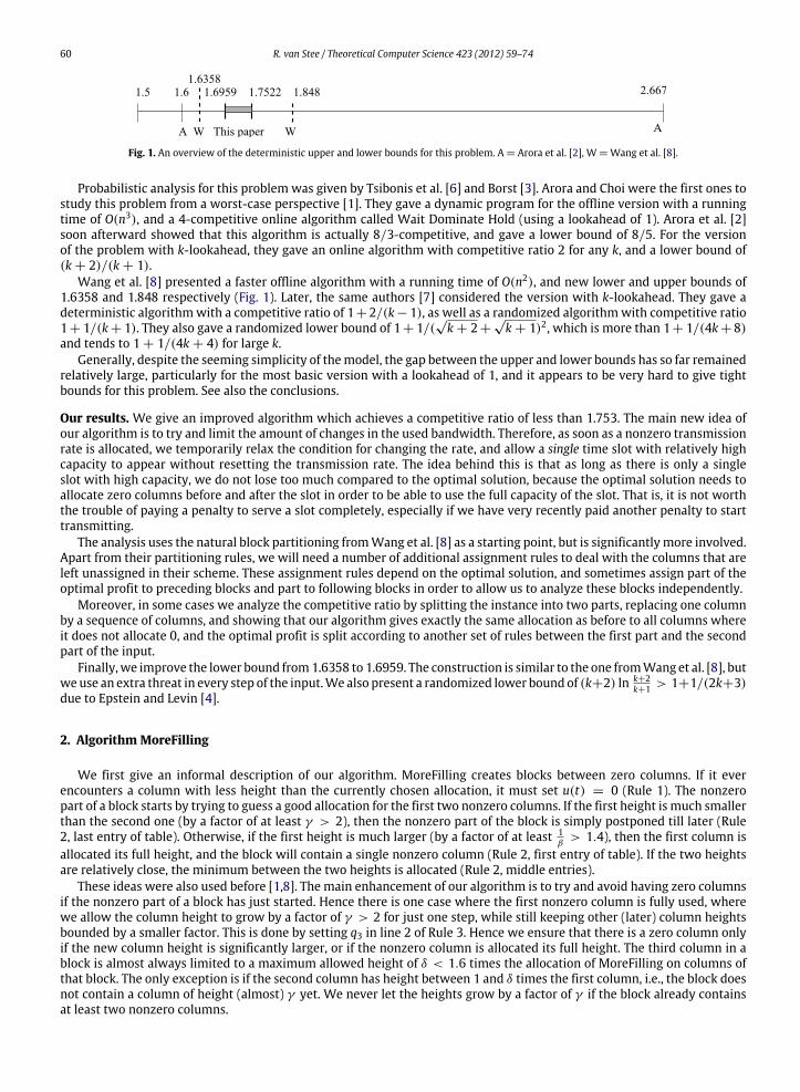
Fig. 1. An overview of the deterministic upper and lower bounds for this problem. A = Arora et al. [2], W = Wang et al. [8].

Probabilistic analysis for this problem was given by Tsibonis et al. [6] and Borst [3]. Arora and Choi were the first ones tostudy this problem from a worst-case perspective [1]. They gave a dynamic program for the offline version with a runningtime of O(n3), and a 4-competitive online algorithm called Wait Dominate Hold (using a lookahead of 1). Arora et al. [2]soon afterward showed that this algorithm is actually 8/3-competitive, and gave a lower bound of 8/5. For the versionof the problem with k-lookahead, they gave an online algorithm with competitive ratio 2 for any k, and a lower bound of(k + 2)/(k + 1).

Wang et al. [8] presented a faster offline algorithm with a running time of O(n2), and new lower and upper bounds of1.6358 and 1.848 respectively (Fig. 1). Later, the same authors [7] considered the version with k-lookahead. They gave adeterministic algorithmwith a competitive ratio of 1+ 2/(k− 1), as well as a randomized algorithmwith competitive ratio1+ 1/(k+ 1). They also gave a randomized lower bound of 1+ 1/(

√k + 2+

√k + 1)2, which is more than 1+ 1/(4k+ 8)

and tends to 1 + 1/(4k + 4) for large k.Generally, despite the seeming simplicity of themodel, the gap between the upper and lower bounds has so far remained

relatively large, particularly for the most basic version with a lookahead of 1, and it appears to be very hard to give tightbounds for this problem. See also the conclusions.

Our results. We give an improved algorithm which achieves a competitive ratio of less than 1.753. The main new idea ofour algorithm is to try and limit the amount of changes in the used bandwidth. Therefore, as soon as a nonzero transmissionrate is allocated, we temporarily relax the condition for changing the rate, and allow a single time slot with relatively highcapacity to appear without resetting the transmission rate. The idea behind this is that as long as there is only a singleslot with high capacity, we do not lose too much compared to the optimal solution, because the optimal solution needs toallocate zero columns before and after the slot in order to be able to use the full capacity of the slot. That is, it is not worththe trouble of paying a penalty to serve a slot completely, especially if we have very recently paid another penalty to starttransmitting.

The analysis uses the natural block partitioning fromWang et al. [8] as a starting point, but is significantlymore involved.Apart from their partitioning rules, we will need a number of additional assignment rules to deal with the columns that areleft unassigned in their scheme. These assignment rules depend on the optimal solution, and sometimes assign part of theoptimal profit to preceding blocks and part to following blocks in order to allow us to analyze these blocks independently.

Moreover, in some cases we analyze the competitive ratio by splitting the instance into two parts, replacing one columnby a sequence of columns, and showing that our algorithm gives exactly the same allocation as before to all columns whereit does not allocate 0, and the optimal profit is split according to another set of rules between the first part and the secondpart of the input.

Finally,we improve the lower bound from1.6358 to 1.6959. The construction is similar to the one fromWang et al. [8], butweuse an extra threat in every step of the input.We also present a randomized lower bound of (k+2) ln k+2

k+1 > 1+1/(2k+3)due to Epstein and Levin [4].

2. AlgorithmMoreFilling

We first give an informal description of our algorithm. MoreFilling creates blocks between zero columns. If it everencounters a column with less height than the currently chosen allocation, it must set u(t) = 0 (Rule 1). The nonzeropart of a block starts by trying to guess a good allocation for the first two nonzero columns. If the first height is much smallerthan the second one (by a factor of at least γ > 2), then the nonzero part of the block is simply postponed till later (Rule2, last entry of table). Otherwise, if the first height is much larger (by a factor of at least 1

β> 1.4), then the first column is

allocated its full height, and the block will contain a single nonzero column (Rule 2, first entry of table). If the two heightsare relatively close, the minimum between the two heights is allocated (Rule 2, middle entries).

These ideas were also used before [1,8]. The main enhancement of our algorithm is to try and avoid having zero columnsif the nonzero part of a block has just started. Hence there is one case where the first nonzero column is fully used, wherewe allow the column height to grow by a factor of γ > 2 for just one step, while still keeping other (later) column heightsbounded by a smaller factor. This is done by setting q3 in line 2 of Rule 3. Hence we ensure that there is a zero column onlyif the new column height is significantly larger, or if the nonzero column is allocated its full height. The third column in ablock is almost always limited to a maximum allowed height of δ < 1.6 times the allocation of MoreFilling on columns ofthat block. The only exception is if the second column has height between 1 and δ times the first column, i.e., the block doesnot contain a column of height (almost) γ yet. We never let the heights grow by a factor of γ if the block already containsat least two nonzero columns.

R. van Stee / Theoretical Computer Science 423 (2012) 59–74 61

Fig. 2. The algorithm MoreFilling, consisting of three rules. The value t1 in Rule 3 is the index of the first nonzero column of the current block, and H is itsbase height (see Definition 2).

We now formally define our algorithm. Define the following values.

R = = 1.75214 β = R/(2R − 1) = 0.69966ε = (2R − 3)β = 0.35282 γ = R/(4 − 2R + ε) = 2.06489δ = (2Rβ − ε − 1)/β = 1.57074 η = 1 − R/γ + ε = 0.50414

We have (5 − R/γ + ε)/(1 + δ) = R. Our algorithm is defined in Fig. 2.

Theorem 1. The competitive ratio of MoreFilling is at most R = 1.75214.

It should be pointed out that δ could be set to any value between roughly 1.55 and 5/3, and MoreFilling would still be1.753-competitive. The other variables, β, ε and γ are decisive.

3. Upper bound analysis

Fix an optimal solution opt. We denote its allocation to column i by a(i). For a set of columns S, let alg(S) denote thetotal profit of algorithm alg on the columns in S. We abbreviate MoreFilling by mf.

We begin our analysis by introducing the block partitioning and giving some properties of the optimal solution inSection 3.1. We use this to analyze the most basic type of block in Theorem 2. The remaining cases are treated inSections 3.2–3.5. A more detailed overview of the cases is given at the end of Section 3.1.

3.1. Block partitioning

We classify the columns with zero allocation (also called zero columns) by the step in which they are set to 0: a columnis of type i if it is set to 0 in Step i of our algorithm. Note that type 2 columns only occur after other zero columns. We followthe partitioning scheme fromWang et al. [8], which we describe next.

A type 1 column ends a block, and is a part of that block. If column i is a type 3 column, one block ends at column i − 1and the next starts at column i + 1. (In this case, we will decide later what to do with column i.) This partitioning schemeignores the type 2 columns (which only occur after other zero columns). Each block hence consists of zero or more type 2columns, followed by one or more nonzero columns and possibly one final type 1 column. For each block B, the number ofnonzero columns in B, also called the length of B, is denoted by |B|.

Let us consider the possible optimal profit on a block. We normalize the height of the columns in this block such that theheight of the first column is exactly 1.

Definition 1. We define the BaseHeight of a block with at least two nonzero columns as the minimum height among itsfirst two nonzero columns.

The BaseHeight is abbreviated by H in the algorithm.

Definition 2. A block is called long if it has at least one (nonzero) column after its first fully-used column, else it is calledshort.

Observation 1. Consider a block of which the first nonzero column is column i. We have h(i) = 1. If h(i) > h(i + 1), thenh(i + 1) ≥ βh(i), or u(i + 1) = 0. If u(i + 1) > 0 and the last column k of this block is of type 1, we have h(k) < β .

If h(i) ≤ h(i + 1), then h(i + 1) < γ . Moreover, almost always we have h(j) < δ for all j > i + 1 such that j and i belong tothe same block. The only exception to this is if h(i+ 1) ≤ δ, in which case we have h(i+ 2) < γ if i+ 2 is part of the same block.In addition, if the last column k of the block of i is of type 1, we have h(k) < β .

We now consider the type 2 zero columns at the start of the block.


Lemma 1 (Wang et al.). Given a sequence of columns S, if the height of each column is at least γ times the height of the previousone (where γ ≥ 2), then opt(S) ≤

γ 2

γ 2−1h where h is the height of the last column in S. This value is achieved by using every other

column completely starting from the right.

In order to efficiently deal with all the cases, we will in fact use the following estimates, which are all higher than thebound from Lemma 1. Consider a column i of height hwhich is preceded by type 2 columns. Wemake two distinctions: onebased on whether a(i) > h/γ or not (if a(i) > h/γ , then a(i − 1) = 0), and one based on whether the block containingcolumn i is long or short (Definition 2). The bounds used are as follows.

a(i) > h/γ a(i) ≤ h/γShort block ε ≈ 0.353 εγ ≈ 0.729Long block η ≈ 0.505 εγ ≈ 0.729

(1)

Naturally the profit on type 2 columns does not really depend on the type of the following block, but this assumptionsimplifies the analysis later.

Observation 2. If the input contains a sequence of columns i, . . . , j such that h(k) ≥ γ h(k − 1) for k = i + 1, . . . , j, thenmf({i, . . . , j − 1}) = 0.

To determine the maximum optimal profit on a block, we need to consider how the type 2 blocks at the start of sucha block are serviced. Depending on the exact heights of the nonzero columns, it may not be optimal to service them asdescribed in Lemma 1. However, Observation 2 allows us to make the following assumption.

Assumption 1. If columns i, . . . , j form a sequence of type 2 columns followed by a nonzero column j, then h(k) = γ h(k−1)for k = i + 1, . . . , j + 1.

Here we conceptually round up column heights starting from the end, leaving h(j) unchanged and defining h(j − 1),h(j − 2), . . . , h(i) by the equality in Assumption 1. This can only improve the total optimal value. Regarding MoreFilling, ifthe previous block ended with a type 1 column, its behavior on the immediately following type 2 columns (and hence theentire input) is unaffected by this change. If that block ended with a type 3 column, then the column following that was toohigh for the block to continue, and this still holds now.

Lemma 2. For each column i, we have a(i) = 0 or a(i) > h(i)/3.

Proof. Suppose the optimal allocation for columns i − 1, i, i + 1 is x, a(i), z (if one of these columns does not exist, assumethat its height is zero), then we have x = 0 or x = a(i) and we also have z = 0 or z = a(i), so if a(i) < h(i)/3 we can replacex, a(i), z by 0, h(i), 0, which is always feasible. �

We have the following lemma which will later simplify the analysis.

Lemma 3. Let S be a sequence of type 2 columns i, . . . , j. Let the height of the final type 2 columnbe h. Let V (S) := opt(S)+η·a(j).If a(i) > 0, then V (S) ≤ εγ 2h.

Proof. By Lemma 2 and Assumption 1, for any column i′ ≥ 1 in S, only three allocations then need to be considered:0, h(i′)/γ , and h(i′).

Let x be the number of columns. If x is odd, the optimal allocation to S is given by Lemma 1, and this satisfies the constraintthat the first column have nonzero allocation. For x = 1, the optimal profit on S is h. To this we add ηh to get V (S), and wehave 1 + η = εγ 2. For any odd x ≥ 3 we have

V (S) = h +hγ 2

+ · · · +h

γ x−1

2 −

R

γ+ ε

(2)

while for x + 2 this value becomes

h + · · · +h

γ x−1+

hγ x+1

2 −

R

γ+ ε

which is less than (2) since γ 2(2 −

Rγ

+ ε) > γ 2+ 2 −

Rγ

+ ε. Therefore, V (S) ≤ εγ 2h for all odd x.


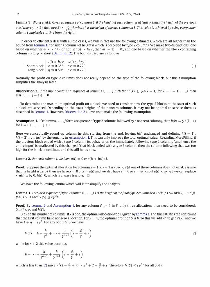
Fig. 3. This figure shows the maximum possible heights of nonzero columns in a block (plus a final type 1 column). There are three cases. Let the firstnonzero column of the block be t , then we have the cases δh(t) < h(t + 1) ≤ γ h(t) (left), h(t) ≤ h(t + 1) ≤ δh(t) (middle), and βh(t) ≤ h(t + 1) < h(t)(right). If h(t + 1) < βh(t), the block contains only a single nonzero column; if h(t + 1) > γ h(t), no block starts at time t . The third column may haveheight γ only if the heights are ascending and the second column has height at most δ. Shown is the case where the sixth column is of type 1; if there areadditional nonzero columns instead, their maximum height is the same as that of the fifth column.

For x = 2, given that the first column (of height hγ) must have nonzero allocation, it is best to assign the same value to

the second column, and we find V (S) ≤1γ 2 (3 −

Rγ

+ ε) < εγ 2h by inspection.Given an instance with x type 2 columns (x is even), consider the instance with x + 2 type 2 columns. Let the height of

column x be h′. If it was optimal to use column x fully, then it is now optimal to use column x + 2 (of height γ 2h′) fully aswell. This adds γ 2h′ to the total profit. The profit on the first x columns cannot be improved (by induction on even x), andthere is no other assignment to column x that increases the profit on the last two columns to a value above γ 2h′. Thus, wedo not need to consider other allocations to column x in this case. Analogously to the case of odd x, we can now show thatV (S) decreases for increasing x. �

Theorem 2. MoreFilling is R-competitive on a block which is not immediately followed by a type 3 column.

Proof. Let first be the index of the first nonzero column in block b, and normalize h(first) = 1. Then, the profit of ouralgorithm on this block is |b| or β|b|, depending on whether h(first) ≤ h(first + 1). By the text below Lemma 1, theoptimal profit on the type 2 columns in b is at most εγ h(first) (the height of the last type 2 column is at most h(first)/γ ,and if the last type 2 column is not used, the optimal profit on the other type 2 columns is at most εh(first), or at mostηh(first) if the block is long). For the calculations, we make the worst-case assumption that there is a type 1 column at theend of this block, and it has height 1 (it actually must have smaller height). The exception to this is a block of length 1; inthat case, the type 1 column must have height at most βh(first) by our algorithm.

Note that all nonzero columns in the block have height at least 1. To derive upper bounds for the optimal profit ona block, we may assume that each of these columns has the maximum height as bounded by Observation 1 (Fig. 3). Theonly allocations that we need to consider to find the optimal profit are values that are the height of at least one column.In particular, for column first, by Lemma 2 only the following allocations need to be considered: h(first), 1

γh(first), and

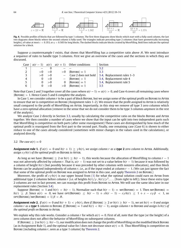
possibly βh(first).This gives us the results shown in Fig. 4. The figure shows the optimal profit for each case and compares it to the profit

of MoreFilling. Regarding a block of length 1 for instance, we find that it is optimal to set a(first) = a(first + 1) =

h(first + 1) ≤ βh(first), a(first − 1) = 0, and then it is possible to earn at most εh(first) < 0.353h(first) on the type 2columns up to column first − 2.

For a block that contains three or more nonzero columns, note that adding a column of height δ (resp. δβ in caseh(first + 1) < h(first)) adds at most δ (resp. δβ) to the optimal profit and exactly 1 (resp. β) to the profit of MoreFilling.Since δ < R, this does not increase the competitive ratio above R. �

To complete our analysis, we now need to eliminate the type 3 columns. These columns are the most difficult to handlefor the following reason. For type 1 columns, MoreFilling already decided in the previous time step (or earlier) to allocatezero to the type 1 column, because its height is too small compared to some previous height. Similarly, type 2 columns areallocated zero because their height is small compared to the immediately following height. For these cases, it is clear howto group the columns into blocks as described above (i.e., how to compensate for the missed profit on the zero column), andwe can analyze these cases in a straightforward way as shown in Theorem 2.

In contrast, type 3 columns are allocated zero ‘‘at the last minute’’, and this decision does not depend on its own height.This is in particular troublesome in the case where column r is a type 3 zero column, and column r − 1 was allocatedh(r) < h(r − 1). In normal cases, column r would be allocated h(r) to compensate for the fact that less than h(r − 1) wasearned on column r −1. But now, column r is allocated zero, and inmany cases wewill have to consider the block followingcolumn r to complete the analysis.

For a type 3 column r , we denote the block immediately preceding it by Before(r) and the block immediately followingit by After(R). We will abbreviate these blocks by Before and After if the meaning is clear from the context (which is mostof the time). When analyzing column r , we always normalize the heights of the columns such that the height of the firstnonzero column of the preceding block Before is 1. Then h(r) ∈ [β, γ ], and if the first column of Before is not fully used orthe second column has height at least δ, we have h(r) ≤ δH , where H is the base height of block Before (else column r − 1would have been zeroed). We also have that

h(r + 1) > δH. (3)


Fig. 4. Possible profiles of blocks that are followed by type 1 columns. The first three diagrams show blocks which start with a fully-used column, the lasttwo diagrams show blocks where the second column is fully-used. The triangles indicate preceding type 2 columns (that have geometrically increasingheights), of value at most ε < 0.353, or η < 0.505 for long blocks. The dashed blocks indicate blocks created byMoreFilling. Bold lines indicate the optimalsolution for a block.

Suppose a counterexample I exists, that shows that MoreFilling has a competitive ratio above R. We next introducea sequence of rules to handle type 3 columns. First we give an overview of the cases and the sections in which they arediscussed.

Case a(r − 1) a(r) a(r + 1) Other conditions Section1 − 0 − − 3.22 >0 >0 >0 |Before| = 1 3.33 >0 >0 − Case 2 does not hold 3.4, Replacement rules 1–34 0 >0 − |Before| > 1 3.4, Replacement rule 45 0 >0 0 |Before| = 1 3.4, Replacement rule 56 0 >0 >0 |Before| = 1 3.5

Note that Cases 2 and 3 together cover all the cases where a(r −1) = a(r) > 0, and Case 4 covers all remaining cases where|Before| > 1. Hence Cases 5 and 6 complete the analysis.

In Case 1, we consider column r to be a part of block Before, but we assign some of the optimal profit on Before to Afterto ensure thatmf is competitive on Before (Assignment rules 1–2). We ensure that the profit assigned to After is relativelysmall compared to the profit of MoreFilling on After. Importantly, in this step we remove all type 3 zero columns whichhave a zero optimal allocation (remove in the sense that we do not consider them to be type 3 columns anymore in the restof the analysis).

We analyze Case 2 directly in Section 3.3, usually by calculating the competitive ratio on the blocks Before and Aftertogether. We then consider a number of cases where we show that the input can be split into two independent parts suchthat MoreFilling is competitive on both parts (after some reassignment) These cases are distinguished by how much of theoptimal profit is reassigned from the first part to the second part. Finally, one remaining case (Case 6) is shown to eitherreduce to one of the cases already considered (sometimes with minor changes in the values used in the calculations), oranalyzed directly.

3.2. The case a(r) = 0

Assignment rule 1. If a(r) = 0 and h(r + 1) ≥ γ h(r), we assign column r as a type 2 zero column to After. Additionally,assign εγ h(r) of the optimal profit on Before to After.

As long as we have |Before| ≥ 2 or h(r) ≥ h(r − 1), this works because the allocation of MoreFilling to column r − 1was not adversely affected by column r . That is, u(r − 1) was not set to a value below h(r − 1) because it was followed bya column of height h(r) (but possibly because it was preceded by other columns with nonzero allocation), and thus blockBefore can be analyzed independently of column r , i.e., as if the input ended at column r − 1. (We can just ignore the factthat some of the optimal profit on Before was assigned to After in this case, and apply Theorem 2 on Before.)

Moreover, the profit of εγ h(r) is our upper bound from (1) for what the optimal solution could earn on After fromadditional type 2 columns before column r (i.e. of heights h(r)/γ , h(r)/γ 2, . . . (from right to left)). Since these extra type2 columns are not in fact present, we can reassign this profit from Before to After. We will use the same idea later in ourreplacement rules (Section 3.4).

Suppose |Before| = 1 and h(r) < h(r − 1). Normalize such that h(r − 1) = mf(Before) = 1. Then mf(Before) =

h(r) ≥ β . Since a(r) = 0, we have opt(Before) ≤ h(r − 1) + εh(r − 1) − εγ h(r) ≤ 1 + ε − εγ β < 1, soopt(Before)/mf(Before) < 1/β < R.

Assignment rule 2. If a(r) = 0 and h(r + 1) < γ h(r), then if |Before| ≥ 2 or h(r) ≥ h(r − 1), we set h(r) = 0 and assigncolumn r as a type 1 column to Before. If |Before| = 1 and h(r) < h(r − 1), assign column r to Before and assign δεh(r) ofthe optimal profit on Before to After.

We explain why this rule works. Consider a column r for which a(r) = 0. First of all, note that the type (or the height) of azero column does not affect the behavior of MoreFilling on subsequent columns.

If |Before| ≥ 2orh(r) ≥ h(r−1), ourmodificationdoes not change theprofit ofMoreFilling on themodified blockBefore(as in Assignment Rule 1), and the optimal value for I does not decrease since a(r) = 0. Thus MoreFilling is competitive onBefore (including column r , seen as a type 1 column) by Theorem 2.


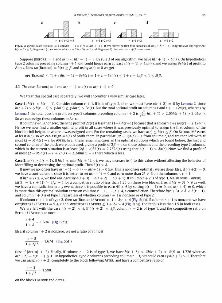
Fig. 5. A special case: |Before| = 1 and a(r − 1) = a(r) = a(r + 1) > 0. We show the first four subcases of h(r) ≥ h(r − 1). Diagrams (a)–(b) representh(r + 2) ≥ δ, diagram (c) the case in which r + 2 is of type 1, and diagram (d) the case that r + 2 is nonzero.

Suppose |Before| = 1 and h(r) < h(r − 1) = 1. By rule 3 of our algorithm, we have h(r + 1) > δh(r). On hypotheticaltype 2 columns preceding column r + 1, opt could hence earn at least εh(r + 1) > δεh(r), and we assign δεh(r) of profit toAfter. Now mf(Before) = h(r) ≥ β , and using a(r) = 0 we get

opt(Before) ≤ (1 + ε)h(r − 1) − δεh(r) = 1 + ε − δεh(r) ≤ 1 + ε − δεβ < 1 < Rβ.

3.3. The case |Before| = 1 and a(r − 1) = a(r) = a(r + 1) > 0

We treat this special case separately; we will encounter a very similar case later.

Case 1: h(r) < h(r − 1). Consider column r + 1. If it is of type 2, then we must have a(r + 2) = 0 by Lemma 2, sinceh(r + 2) > γ h(r + 1) > γ δh(r) ≥ γ δa(r) > 3a(r). But the total optimal profit on columns r and r + 1 is 2a(r), whereas byLemma 1 the total possible profit on type 2 columns preceding column r + 2 is γ 2

γ 2−1h(r + 1) > 2.05h(r + 1) ≥ 2.05a(r).

So we can assign these columns to After.If column r+1 is nonzero, then theprofit of 2a(r) is less than (1+ε)h(r+1)because that is at least (1+ε)δa(r) = 2.12a(r).

Hence we now find a smaller optimal profit in all cases where it was previously optimal to assign the first column of theblock its full height, or where it was assigned zero. For the remaining cases, we have a(r) ≤ h(r) ≤ β . On Before, MF earnsat least h(r), so we can assign Rh(r) of profit there, in particular (R − 1)h(r) − ε from column r , and are then left with atmost (2 − R)h(r) − ε for After. In all these remaining cases, in the optimal solutions which we found before, the first andsecond column of the block were both used, giving a profit of 2β + ε on those columns and the preceding type 2 columns,which in the current situation is at least (2β + ε)δh(r) = 2.752h(r) using that h(r + 1) > δh(r). Now, we find a profit ofat most (2 − R)h(r) − ε + 2h(r) = 2.248h(r) − ε there which is less.

Case 2: h(r) ≥ h(r − 1). If h(r) < min(h(r + 1), γ ), we may increase h(r) to this value without affecting the behavior ofMoreFilling or decreasing the optimal profit. Then h(r) > δ.

If nowwe no longer have a(r−1) = a(r) = a(r+1) > 0 (i.e., this is no longer optimal), we are done. Else, if a(r+2) = 0,we have a contradiction, since it is better to set a(r − 1) = 0 and earn more than 2δ > 3 on the columns r, r + 1.

If h(r + 2) ≥ δ, we find analogously a(r + 3) = a(r + 2) = a(r + 1). If column r + 2 is of type 1,mf(Before∪ After) =

mf({r − 1, r + 1}) ≥ δ/β + 1 for a competitive ratio of less than 1.25 on these two blocks. Else, if h(r + 3) ≥ δ as well,we have a contradiction in any event, since it is possible to earn 4δ > 6 by setting a(r − 1) = 0 and a(r + 4) = 0, whichis more than this optimal solution earns on columns r − 1, . . . , r + 4, a contradiction. Therefore h(r + 3) < δ < h(r + 1),and column r + 3 is of type 1, regardless of whether column r + 1 is nonzero or of type 2.

If column r + 1 is of type 2, then mf(Before ∪ After) > 1 + δγ > 4 (Fig. 5(a)). If column r + 1 is nonzero, we haveopt(Before ∪ After) = 5 + ε and mf(Before ∪ After) ≥ 1 + 2δ > 4 (Fig. 5(b)). The ratio is less than 1.5 in both cases.

We are left with the case h(r + 2) < δ. If h(r + 2) < δβ , column r + 2 is of type 1, and the competitive ratio onBefore ∪ After is at most

ε + 41 + δ

= 1.694 (Fig. 5(c)).

Else, if column r + 2 is nonzero, we get a ratio of at most

ε + 51 + 2βδ

= 1.674 (Fig. 5(d))

(less if |After| > 2). Finally, if column r + 2 is of type 3, we have h(r + 3) > δh(r + 2) > δ2β = 1.726 whereasa(r +2) = a(r −1) ≤ 1. On hypothetical type 2 columns preceding column r +3, opt could earn εγ h(r +3) > 1. Thereforewe can assign a(r + 2) completely to the block following After, and have a competitive ratio of

ε + 31 + βδ

= 1.598

on the blocks Before and After.


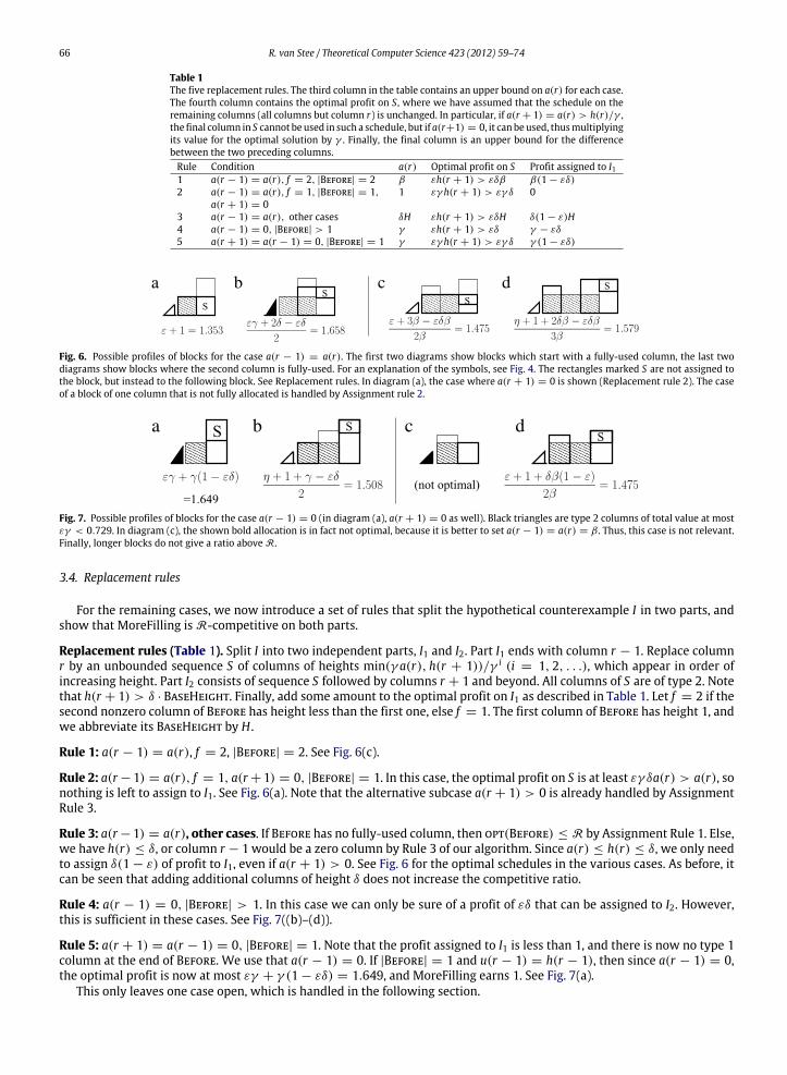
Table 1The five replacement rules. The third column in the table contains an upper bound on a(r) for each case.The fourth column contains the optimal profit on S, where we have assumed that the schedule on theremaining columns (all columns but column r) is unchanged. In particular, if a(r + 1) = a(r) > h(r)/γ ,the final column in S cannot beused in such a schedule, but if a(r+1) = 0, it canbeused, thusmultiplyingits value for the optimal solution by γ . Finally, the final column is an upper bound for the differencebetween the two preceding columns.Rule Condition a(r) Optimal profit on S Profit assigned to I11 a(r − 1) = a(r), f = 2, |Before| = 2 β εh(r + 1) > εδβ β(1 − εδ)

2 a(r − 1) = a(r), f = 1, |Before| = 1, 1 εγ h(r + 1) > εγ δ 0a(r + 1) = 0

3 a(r − 1) = a(r), other cases δH εh(r + 1) > εδH δ(1 − ε)H4 a(r − 1) = 0, |Before| > 1 γ εh(r + 1) > εδ γ − εδ

5 a(r + 1) = a(r − 1) = 0, |Before| = 1 γ εγ h(r + 1) > εγ δ γ (1 − εδ)

Fig. 6. Possible profiles of blocks for the case a(r − 1) = a(r). The first two diagrams show blocks which start with a fully-used column, the last twodiagrams show blocks where the second column is fully-used. For an explanation of the symbols, see Fig. 4. The rectangles marked S are not assigned tothe block, but instead to the following block. See Replacement rules. In diagram (a), the case where a(r + 1) = 0 is shown (Replacement rule 2). The caseof a block of one column that is not fully allocated is handled by Assignment rule 2.

Fig. 7. Possible profiles of blocks for the case a(r − 1) = 0 (in diagram (a), a(r + 1) = 0 as well). Black triangles are type 2 columns of total value at mostεγ < 0.729. In diagram (c), the shown bold allocation is in fact not optimal, because it is better to set a(r − 1) = a(r) = β . Thus, this case is not relevant.Finally, longer blocks do not give a ratio above R.

3.4. Replacement rules

For the remaining cases, we now introduce a set of rules that split the hypothetical counterexample I in two parts, andshow that MoreFilling is R-competitive on both parts.

Replacement rules (Table 1). Split I into two independent parts, I1 and I2. Part I1 ends with column r − 1. Replace columnr by an unbounded sequence S of columns of heights min(γ a(r), h(r + 1))/γ i (i = 1, 2, . . .), which appear in order ofincreasing height. Part I2 consists of sequence S followed by columns r + 1 and beyond. All columns of S are of type 2. Notethat h(r + 1) > δ · BaseHeight. Finally, add some amount to the optimal profit on I1 as described in Table 1. Let f = 2 if thesecond nonzero column of Before has height less than the first one, else f = 1. The first column of Before has height 1, andwe abbreviate its BaseHeight by H .

Rule 1: a(r − 1) = a(r), f = 2, |Before| = 2. See Fig. 6(c).

Rule 2: a(r −1) = a(r), f = 1, a(r +1) = 0, |Before| = 1. In this case, the optimal profit on S is at least εγ δa(r) > a(r), sonothing is left to assign to I1. See Fig. 6(a). Note that the alternative subcase a(r + 1) > 0 is already handled by AssignmentRule 3.

Rule 3: a(r −1) = a(r), other cases. If Before has no fully-used column, then opt(Before) ≤ R by Assignment Rule 1. Else,we have h(r) ≤ δ, or column r − 1 would be a zero column by Rule 3 of our algorithm. Since a(r) ≤ h(r) ≤ δ, we only needto assign δ(1 − ε) of profit to I1, even if a(r + 1) > 0. See Fig. 6 for the optimal schedules in the various cases. As before, itcan be seen that adding additional columns of height δ does not increase the competitive ratio.

Rule 4: a(r − 1) = 0, |Before| > 1. In this case we can only be sure of a profit of εδ that can be assigned to I2. However,this is sufficient in these cases. See Fig. 7((b)–(d)).

Rule 5: a(r + 1) = a(r − 1) = 0, |Before| = 1. Note that the profit assigned to I1 is less than 1, and there is now no type 1column at the end of Before. We use that a(r − 1) = 0. If |Before| = 1 and u(r − 1) = h(r − 1), then since a(r − 1) = 0,the optimal profit is now at most εγ + γ (1 − εδ) = 1.649, and MoreFilling earns 1. See Fig. 7(a).

This only leaves one case open, which is handled in the following section.


3.5. The final case

Due to our calculations so far, we only need to deal with the following remaining case:

|Before| = 1, u(r − 1) = h(r − 1), a(r − 1) = 0 and a(r + 1) = a(r) > 0. (4)

(The case u(r −1) = h(r) < h(r −1)was handled by Assignment Rule 2.) In this unresolved case, the first question we haveis how much of the optimal profit on column r must be assigned to block After (since if it were all counted as part of theoptimal profit on block Before, MoreFilling would not be competitive on Before). Let x be the number of type 2 columnsimmediately following column r , and let r2 be the index of the zero column immediately following |After|.

Lemma 4. The profit that is assigned forward from column r in the case described in (4) is at most (1 −Rγ

+ ε)a(r) = ηa(r).Normalizing such that the first nonzero column of After has height 1, this is at most η/γ x.

Proof. We have a(r) ≤ min(h(r), h(r + 1)). We assign (R/γ − ε)a(r) ≤ (R/γ − ε)h(r) ≤ (R − εγ )h(r − 1) to Before(to add to the εγ h(r − 1) from the type 2 columns) and are left with (1 −

Rγ

+ ε)a(r) ≤ (1 −Rγ

+ ε)h(r + 1). The lemmafollows because the sequence of type 2 columns has (at least) geometrically increasing heights. In particular, if x = 0, weuse that a(r) ≤ h(r + 1), and h(r + 1) = 1 in this case. �

Using Lemma 3, we have that if x ≥ 1, we get exactly the value εγ for the type 2 columns plus this forward assignmentfrom column r , which is the value that we have been calculating with in case the last type 2 column had nonzero allocationin the optimal solution. Thus, we get exactly the same analysis as before, with the difference (for x = 1) that opt is requiredto use the type 2 column by assumption. Clearly, if we remove this requirement (and generally use the bound ε > η/γ incase opt does not use the final type 2 column), we can only get higher bounds for the competitive ratio. Hence, our previousanalysis holds unless x = 0, i.e., there are no type 2 columns before After. (Of course, if for After we encounter the opencase that we are discussing in this section, we just repeat; eventually we reach the end of the sequence or find a case whichwe can prove.) In the case x = 0, the optimal solution must use the first nonzero column of After (as well as the precedingcolumn). We summarize this discussion in the following lemma.

Lemma 5. In the remaining open case, column r + 1 is the first nonzero column of block After, and a(r + 1) = a(r).

Lemma 6. MoreFilling is competitive on After even after taking the forward assignment from column r into account, unless|After| = 1 and a(r − 1) = a(r) = a(r + 1).

Proof. If After is a long block, we already calculated with an optimal profit of at least η on the type 2 columns in all casesand are done. Else if After is followed by a type 3 column r2, we see in Figs. 6 and 7 that MoreFilling is still R-competitive ifthe profit on preceding columns is η instead of ε (or εγ ) apart from in the excluded case. If After is not followed by a type3 column, then if |After| = 1 we get a ratio of at most (2β + ηβ) = R, using that a(r + 1) = a(r) ≤ β and Lemma 4. If|After| = 2 and f = 2, then if a(r + 1) = a(r + 2) as in Fig. 4, we find a ratio of at most (3a(r) + ηa(r))/(2a(r)) = R sincenow a(r) ≤ u(r + 2). Else, the ratio is at most (η + 1 + β)/(2β) < 1.6. �

We are left with the case |After| = 1, so r2 = r + 2 and a(r − 1) = · · · = a(r + 2) since type 3 columns have nonzerooptimal allocation. Since r2 is of type 3,

h(r2 + 1) > δh(r2 − 1) = δh(r + 1) ≥ δa(r). (5)

If a(r2 + 1) = 0, we apply our Replacement rule 2, i.e., column r2 is assigned completely to the block following After. Thisworks because on (hypothetical) type 2 columns preceding column r2+1, opt could earn εγ h(r2+1) > h(r2+1)/δ > a(r2).We then have opt(After) ≤ 1 + (1 −

Rγ

+ ε) < 1.51.Else, we are again in the case discussed in Section 3.3, since a(r2 − 1) = a(r2) = a(r2 + 1). The only difference is that the

profit from previous columns is not ε but η. We can therefore follow that analysis completely and adjust the calculationswhere necessary. The highest ratio that we found there is (4 + ε)/(1 + δ), and this now becomes (4 + η)/(1 + δ) = R.

4. Lower bounds

4.1. Deterministic lower bound

We let ε > 0 be some very small value. Denote the online algorithm by alg and assume that it has a competitive ratio ofat most (1− ε)1.69595. In our lower bound construction, the adversary uses the following strategy. See Fig. 8. The values pand q are fixed constants which we will determine later; we have p < 1 and q > 2. Each rectangle represents a state. Thestates consist of three components: the current online allocation, the current column, and the next column. Hence, if wemove from one state to another, the second column in the starting state is identical to the first column in the destinationstate. However, we sometimes (conceptually) rescale column heights, for instance when we move from state B to state A.

Additionally, the number (1 − δ)x in the ellipse indicates that one final column of height (1 − δ)x arrives, where x is the(nonzero) allocation that alg just used. Hence, this column has no value for alg (it can only use the column by forfeiting aprofit of x on the current column). Overall, we have the following states.


Fig. 8. Lower bound strategy. The first number in states A–C represents the last allocation of alg and the other two are the two currently visible columns.The variable x always indicates the allocation chosen by alg. At the state change marked with (*), we may change q to q′

= 2.03644 and p to p′= 1/q′ .

State change I (resp. IV) occurs if alg remains in state A (resp. B) ‘‘too long’’ (see Claims 2, 3). State changes II and III occur if alg allocates a ‘‘too low’’ valuex in state A (Lemmas 7, 8).1 The precise conditions for these state changes are given in the mentioned claims and lemmas; we also show that one of thestate changes I–IV always occurs eventually. State change IV can happen both on an allocation of 0 and on an allocation of x.

State DescriptionA The online algorithmallocated 0 to the previous column (or there is no previous column). The visible input

is 1, q (current column, next column).B The online algorithm allocated a nonzero value to the previous column. The visible input is q, q.C The online algorithm allocated 0 to the previous column. The visible input is 1, p.D The online algorithm allocated a nonzero value x to the previous column. A new column of height (1−δ)x

arrives.STOP The input ends: the visible input is the last column of the previous state.

In total, there are in fact 8 possible states (counting D as one state), since states A–C occur in two forms: dependingon the behavior of the online algorithm, the adversary may once (permanently) change the values of q and p to q′ and p′,respectively.

The input. The input starts in state A. The default state changes are given by the normal arrows. As alg is processing theinput, moving between states A and B, the adversary keeps track of the total online profit so far, as well as of the total optimalprofit. When going from state B to A, the adversary may elect to change the value of q to q′

= 2.036442 and p to p′= 1/q′

(for future columns); we will specify when this happens. In both state A and B, nonstandard state changes are possible,which are indicated by dotted lines in Fig. 8. The adversary forces such a state change as soon as this gives the desired lowerbound. Note that in all of the cases where a dotted line is followed, the input consists of at most two more columns, and itis straightforward to calculate the resulting competitive ratio, based on the stored optimal and online profits.

For instance, if alg allocates a certain value x > 0 in state A or B, and the adversary sees that this is too low to maintainthe competitive ratio (because of earlier choices), the input sequence stops immediately. In state B, this may also happenwhen the algorithm allocates 0; hence, there is no condition next to the outgoing dotted line from B. In state A, instead ofstopping immediately, one final column of height (1 − δ)x may arrive, so the adversary has two options here (besides thedefault state change to B) if alg allocates a nonzero value.

What we need to show is that no matter what alg does, at some point the adversary can choose a nonstandard statechange and prove the desired competitive ratio: alg cannot stay in states A and B forever.

Output of the adversary.We first describe how the adversary handles the input as long as alg stays in A and B. This is verysimple: in state A, it allocates 0 if alg allocates x > 0, and alternates between the full column height and 0 otherwise (endingwith 0 when alg allocates a nonzero value). In state B, it always allocates the full column height, except for one special casewhen the input is about to end. In that case, the allocation in state Bwill be the same as on the columns following it.

Claim 1. This output is a feasible solution.

Proof. We only need to show that the adversary does not allocate two different nonzero values to adjacent columns. Giventhe above rules, this could only happen at a state change. In a move from A to B, the adversary always assigns 0. In a movefrom B to A (say at column i), the adversary allocates the full column height, andmay also do this on column i+1, dependingon whether there is an odd or an even number of consecutive state A columns following. But columns i and i + 1 have thesame height here. �

1 If the conditions given in Lemmas 7 and 8 are both satisfied, the adversary could force either change; to fully specify the lower bound strategy, we saythat it uses state change III in such cases.


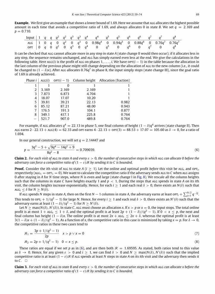
Example. We first give an example that shows a lower bound of 1.69. Herewe assume that alg allocates the highest possibleamount in each time that avoids a competitive ratio of 1.69, and always allocates 0 in state B. We set q = 2.169 andp = 0.710.

Input 1 q q q2 q2 q3 q3 q4 q4 q5 q5 q6 q6 q7 q7 q8

alg 1 0 q 0 q2 0 q3 0 0.98q4 0 0.94q5 0 0.88q6 0 0.76q7 0.76q7

opt 0 q 0 q2 0 q3 0 q4 0 q5 0 q6 0 q7 0 q8

It can be checked that alg cannot allocate more in any step in state A (state change II would then occur); if it allocates less inany step, the sequence remains unchanged, and alg has simply earned even less at the end. We give the calculations in thefollowing table. Here alg(i) is the profit of alg on phases 1, . . . , i. We have opt(i − 1) in the table because the allocation inthe last column of the previous phase might still change depending on the allocation of alg to the new column (i.e., it couldbe changed to (1 − δ)x). After alg allocates 0.76q7 in phase 8, the input simply stops (state change III), since the goal ratioof 1.69 is already achieved.

Phase i alg(i) opt(i − 1) Column height Allocation (fraction)1 1 0 1 12 3.169 2.169 2.169 13 7.873 6.873 4.704 14 18.07 17.07 10.20 15 39.81 39.21 22.13 0.9826 85.12 87.21 48.00 0.9437 176.5 191.3 104.1 0.8778 349.1 417.1 225.8 0.764− 521.7 907.0 489.8 0.764

For example, if alg allocates q4 = 22.13 in phase 5, one final column of height (1 − δ)q4 arrives (state change II). Thenalg earns 2 · 22.13 + alg(4) = 62.33 and opt earns 4 · 22.13 + opt(3) = 88.53 + 17.07 = 105.60 as δ → 0, for a ratio of1.694.

In our general construction, we will set q = 2.14447 and

p =3q2 − 5 +

9q4 − 14q2 + 9

8q2 − 8= 0.709039. (6)

Claim 2. For each visit of alg to state A and every ε > 0, the number of consecutive steps in which alg can allocate 0 before theadversary can force a competitive ratio of (1 − ε)R by sending it to C is bounded.

Proof. Consider the ith visit of alg to state A (i ≥ 1). Let the online and optimal profit before this visit be algi and opti,respectively (alg1 = opt1 = 0). Wewant to calculate the competitive ratio if the adversary sends alg to C when alg assigns0 after staying in A for N time steps, where N is even and large (state change I in Fig. 8). We rescale all the column heightssuch that the columns in state C have heights exactly 1 and p < 1. During the steps that alg spends in state A on its ithvisit, the column heights increase exponentially. Hence, for each i ≥ 1 and each real δ > 0, there exists an N(δ) such thatalgi ≤ δ for N ≥ N(δ).

If alg spends N steps in state A, then on the first N − 1 columns in state A, the adversary earns at least opti +N/2

j=1 q−2j.This tends to opti + 1/(q2 − 1) for large N . Hence, for every i ≥ 1 and each real δ > 0, there exists an N ′(δ) such that theadversary earns at least (1 − δ)/(q2 − 1) for N ≥ N ′(δ).

Let N ≥ max(N(δ),N ′(δ)). In state C , algmust choose an allocation x. If x > p or x = 0, the input stops. The total onlineprofit is at most 1 + algi ≤ 1 + δ, and the optimal profit is at least 2p + (1 − δ)/(q2 − 1). If 0 < x ≤ p, the next andfinal column has height (1 − δ)x. The online profit is at most 2x + algi ≤ 2x + δ, whereas the optimal profit is at least3(1 − δ)x + (1 − δ)/(q2 − 1). As a function of x, the competitive ratio in this case is minimized by taking x = p. For δ → 0,the competitive ratios in these two cases tend to

R1 =3p + 1/(q2 − 1)

2px > p ∨ x = 0 (7)

R2 = 2p + 1/(q2 − 1) 0 < x ≤ p. (8)

These ratios are equal if we set p as in (6), and are then both R = 1.69595. As stated, both ratios tend to this valueas δ → 0. Hence, for any given ε > 0 and i ≥ 1, we can find δ > 0 and N ≥ max(N(δ),N ′(δ)) such that the impliedcompetitive ratio is at least (1 − ε)R if alg spends at least N steps in state A on its ith visit and the adversary then sends itto C . �

Claim 3. For each visit of alg to state B and every ε > 0, the number of consecutive steps in which alg can allocate x before theadversary can force a competitive ratio of (1 − ε)R by sending it to C is bounded.


Proof. In each step in state B, given the above strategy of the adversary, the ratio of the adversary’s profit to the onlineprofit is at least q > 2. Thus, after sufficiently many consecutive columns in state B (depending on the profit of alg and ofthe adversary before the current visit to B), the overall competitive ratio gets arbitrarily close to q > 2 > 1.69595. �

Phases. Given the previous two claims, we know that alg must move back and forth between states A and B, and cannotstay in one state indefinitely. We partition the input into phases. A new phase starts at the start of the input and wheneveralg arrives in state A from state B. We say that a column i is of state A (B) if alg is in state A (B) when it allocates the valuefor column i. Hence a phase always ends with a state B column in which alg allocates 0, unless the input stops in state B.In each phase i, alg allocates exactly one nonzero value (namely when it moves from state A to state B), possibly to someconsecutive columns.

Definition 3. Let 0 < xi ≤ 1 be the fraction of the height of the first column to which alg allocates a nonzero value inphase i.

Claim 4. In each phase but the last, the adversary earns at least q times as much as alg. This profit ratio is monotonicallynondecreasing as a function of the number of state A columns in the phase.

Proof. For a given phase j, scale the column heights in this phase so that the last column (say column i) in state A hasheight 1. Let the number of columns in state B be b ≥ 1. Then alg earns bxj ≤ b whereas the adversary earns at leastbq, namely on columns i + 1, . . . , i + b. The end of this phase looks as follows. Allocations that cause state changes areunderlined.

Input . . . q−3 q−2 q−1 1 q . . . q qState A A A A A B . . . B Balg . . . 0 0 0 xj xj . . . xj 0opt . . . q−3 0 q−1 0 q . . . q q

b columns

(9)

This proves that the profit ratio is at least q and grows as a function of the number of state A columns. �

Corollary 1. W.l.o.g., alg never stays in state B for more than one column.

Proof. On all state B columns, the adversary earns at least q > 2 times as much as alg, as can be seen in Table (9). If alghas a competitive ratio of at most R < 2, then it certainly also has this ratio if it always leaves state B immediately, insteadof staying there for some steps. Thus avoiding extra state B columns can only help alg; note such columns do not affect thecolumn heights of future columns. �

Let alg(j) (opt(j)) be the total profit of alg (opt) after j phases, scaled such that the last state A column in phase j hasheight 1.

Claim 5. As j → ∞, opt(j) → q3/(q2 − 1) = 2.74 or more.

Proof. Given that the last stateA column in phase jhas height 1, the height of all the previous columnswould beminimized iftheywere all of state A: moving backwards from the last column, every time there is a column of state A the height is dividedby q, whereas it remains constant in columns of state B. In this case, shown in Table (9), opt(j) is at least q+ q−1

+ q−3+· · ·

which tends to q3/(q2 − 1). Any state B columns that occur can only increase the optimal profit, since the column heightsincrease. �

Lemma 7. For all j ≥ 1, if alg is R-competitive, we have xj > q/(2R) > 0.6.

Proof. We consider the competitive ratio if the input stops on a nonzero allocation xj in state A (state change III in Fig. 8). Theadversary earns q on the final column of the input, whereas alg earns at most another xj there. By Claim 4, the competitiveratio is at least

q + q · alg(j − 1)2xj + alg(j − 1)

≥ R for xj ≤q

2R.

(For j = 1, we have alg(j − 1) = 0.) �

Wenow first deal with the casewhere after an arbitrary prefix, alg never spends two consecutive steps in the same state,thus from some point onwards each phase is of the form AB. We then get an input and output of the following form (usingthe adversary strategy defined above). Here we normalize such that the first column height in phase n is 1.

Input q1−n q2−n q2−n q3−n . . . q−1 1 1 qState A B A B . . . A B A BPhase 1 2 . . . n − 1 nalg x1q1−n 0 x2q2−n 0 . . . xn−1q−1 0 xn 0opt 0 q2−n 0 q3−n . . . 0 1 0 q


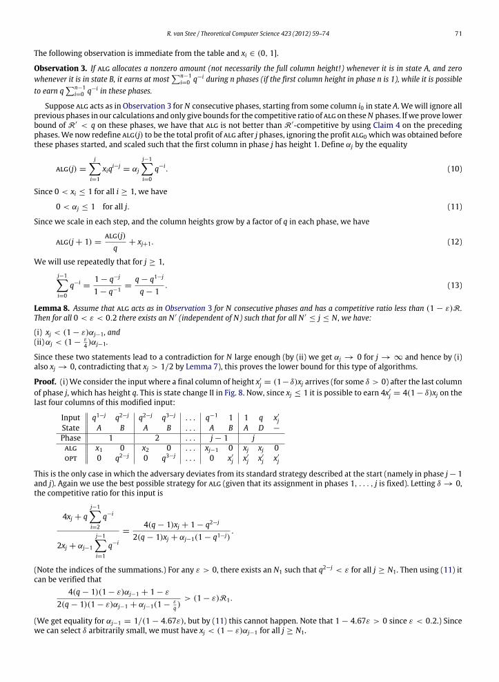
The following observation is immediate from the table and xi ∈ (0, 1].

Observation 3. If alg allocates a nonzero amount (not necessarily the full column height!) whenever it is in state A, and zerowhenever it is in state B, it earns at most

n−1i=0 q−i during n phases (if the first column height in phase n is 1), while it is possible

to earn qn−1

i=0 q−i in these phases.

Suppose alg acts as in Observation 3 for N consecutive phases, starting from some column i0 in state A. Wewill ignore allprevious phases in our calculations and only give bounds for the competitive ratio of alg on theseN phases. If we prove lowerbound of R′ < q on these phases, we have that alg is not better than R′-competitive by using Claim 4 on the precedingphases.We now redefine alg(j) to be the total profit of alg after j phases, ignoring the profit alg0 whichwas obtained beforethese phases started, and scaled such that the first column in phase j has height 1. Define αj by the equality

alg(j) =

ji=1

xiqi−j= αj

j−1i=0

q−i. (10)

Since 0 < xi ≤ 1 for all i ≥ 1, we have

0 < αj ≤ 1 for all j. (11)

Since we scale in each step, and the column heights grow by a factor of q in each phase, we have

alg(j + 1) =alg(j)

q+ xj+1. (12)

We will use repeatedly that for j ≥ 1,j−1i=0

q−i=

1 − q−j

1 − q−1=

q − q1−j

q − 1. (13)

Lemma 8. Assume that alg acts as in Observation 3 for N consecutive phases and has a competitive ratio less than (1 − ε)R.Then for all 0 < ε < 0.2 there exists an N ′ (independent of N) such that for all N ′

≤ j ≤ N, we have:

(i) xj < (1 − ε)αj−1, and(ii)αj < (1 −

ε4 )αj−1.

Since these two statements lead to a contradiction for N large enough (by (ii) we get αj → 0 for j → ∞ and hence by (i)also xj → 0, contradicting that xj > 1/2 by Lemma 7), this proves the lower bound for this type of algorithms.

Proof. (i) We consider the input where a final column of height x′

j = (1− δ)xj arrives (for some δ > 0) after the last columnof phase j, which has height q. This is state change II in Fig. 8. Now, since xj ≤ 1 it is possible to earn 4x′

j = 4(1− δ)xj on thelast four columns of this modified input:

Input q1−j q2−j q2−j q3−j . . . q−1 1 1 q x′

jState A B A B . . . A B A D −

Phase 1 2 . . . j − 1 jalg x1 0 x2 0 . . . xj−1 0 xj xj 0opt 0 q2−j 0 q3−j . . . 0 x′

j x′

j x′

j x′

j

This is the only case in which the adversary deviates from its standard strategy described at the start (namely in phase j− 1and j). Again we use the best possible strategy for alg (given that its assignment in phases 1, . . . , j is fixed). Letting δ → 0,the competitive ratio for this input is

4xj + qj−1i=2

q−i

2xj + αj−1

j−1i=1

q−i

=4(q − 1)xj + 1 − q2−j

2(q − 1)xj + αj−1(1 − q1−j).

(Note the indices of the summations.) For any ε > 0, there exists an N1 such that q2−j < ε for all j ≥ N1. Then using (11) itcan be verified that

4(q − 1)(1 − ε)αj−1 + 1 − ε

2(q − 1)(1 − ε)αj−1 + αj−1(1 −εq )

> (1 − ε)R1.

(We get equality for αj−1 = 1/(1 − 4.67ε), but by (11) this cannot happen. Note that 1 − 4.67ε > 0 since ε < 0.2.) Sincewe can select δ arbitrarily small, we must have xj < (1 − ε)αj−1 for all j ≥ N1.


(ii) We first verify thatαj

q·

qq − 1

+ (1 − ε)αj <1 −

ε

2

αj ·

qq − 1

for q = 2.144472, for any αj > 0 and ε > 0 (the inequality reduces to q/(2q − 2) < 1). Using (10), (12), (13) and (i), thisshows that

alg(j + 1) =αj

q

j−1i=0

q−j+ xj+1 <

1 −

ε

2

αj ·

qq − 1

for j ≥ N1 + 1. By (10) and (13), for every ε > 0 there exists an N2 such that alg(j + 1) > αj+1q

q−1/(1 + ε/4) for all j ≥ N2.Hence for all j ≥ max(N1 + 1,N2), we get

αj+1 <1 −

ε

2

αj

1 +

ε

4

<1 −

ε

4

αj.

We can now define N ′= max(N1 + 1,N2). �

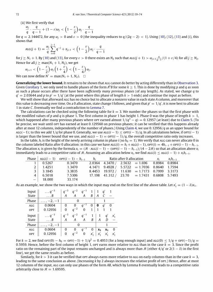
Generalizing the lower bound. It remains to be shown that alg cannot do better by acting differently than in Observation 3.Given Corollary 1, we only need to handle phases of the form AkB for some k ≥ 1. This is done by modifying p and q as soonas such a phase occurs after there have been sufficiently many previous phases (of any length). As stated, we change q toq′

= 2.03644 and p to p′= 1/q′ (at the point where this phase of length k > 1 ends) and continue the input as before.

Wewill show that afterward alg has no choice but to allocate a nonzero value in each state A column, andmoreover thatthis value is decreasing over time. On a 0 allocation, state change I follows, and given that p′

= 1/q′, it is now best to allocate1 in state C . Eventually we find a contradiction to Lemma 7.

The calculations can be checked using the following table for k = 3. We number the phases so that the first phase withthe modified values of p and q is phase 1. The first column in phase 1 has height 1. Phase 0 was the phase of length k > 1,which happened after many previous phases where opt earned almost 1/(q3 − q) = 0.12957 (at least) due to Claim 5. (Tobe precise, we wait until opt has earned at least 0.129560 on previous phases; it can be verified that this happens alreadyafter at most 12 columns, independently of the number of phases.) Using Claim 4, we use 0.12956/q as an upper bound foralg(−1); to this we add 1/q for phase 0. Generally, we use alg(i− 1) ≤ opt(i− 1)/q. In all calculations below, if opt(i− 1)is larger than the lower bound that we use, and alg(i − 1) = opt(i − 1)/q, the overall competitive ratio only increases.

In the table, hi is the height of the newly arriving column in phase i (so h0 = 1). We verify that alg can never allocate 0 inthe column labeled Ratio after 0 allocation: in this case we have alg(i) = hi +alg(i−1), opt(i) = 4hi−1 +opt(i−1)−hi−1.The allocation xi is given by the formula xi = (R · alg(i − 1) − (opt(i − 1) − hi−1)/(4 − 2R) so that an allocation above xiimmediately leads to a competitive ratio of R. Assuming an allocation below xi, we find alg(i) ≤ alg(i − 1) + xihi−1.

Phase alg(i − 1) opt(i − 1) − hi−1 hi Ratio after 0 allocation xi xihi−11 0.5267 0.3470 2.0364 4.3470 / 2.5632 = 1.696 0.8984 0.89842 1.4251 1.3470 4.1471 9.4928 / 5.5722 = 1.7036 0.8640 1.75943 3.1845 3.3835 8.4453 19.972 / 11.630 = 1.7173 0.7999 3.31734 6.5018 7.5306 17.198 41.312 / 23.70 = 1.7431 0.6808 5.7493− 18.000 33.174

As an example, we show the two ways in which the input may end on the first line of the above table. Let x′

1 = (1 − δ)x1.

Input . . . q−3 q−3 q−2 q−1 1 1 q′ 1State . . . B A A A B A C −

Phase . . . , −2, −1 0 1alg 0.0604 0 0 q−1 0 0 q′ 0opt 0.12956 0 q−2 0 1 1 1 1

Input . . . q−3 q−3 q−2 q−1 1 1 q′ x′

1State . . . B A A A B A D −

Phase . . . , −2, −1 0 1alg 0.0604 0 0 q−1 0 x1 x1 0opt 0.12956 0 q−2 0 x′

1 x′

1 x′

1 x′

1

For k = 2, we find opt(0) − h0 = opt(−1) + 1/q2 = 0.4953 (for a long enough input) and alg(0) ≤ 1/q + opt(−1)/q =

0.5959. Hence, before the first column of height 1, opt earns more relative to alg than in the case k = 3. Since the profitratio on the remaining part of the input remains unchanged and is always more than R (either 4/q′ or 2(1 − δ) in the firstline), we get the same results as before.

Similarly, for k > 3 it can be verified that opt always earns more relative to alg on early columns than in the case k = 3,leading to the same conclusion as above. (Increasing k by 2 always increases the relative profit of opt.) Hence, after at most12 columns of the input, alg can only use phases of the form AB, which by Lemma 8 eventually leads to a competitive ratioarbitrarily close to R = 1.69595.


4.2. Randomized lower bound

This lower bound is due to Leah Epstein and Asaf Levin [4] and is published here with their permission. Let k be the sizeof the lookahead window.

Theorem 3. The competitive ratio of any randomized algorithmwith k > 0 is at least (k+2) ln k+2k+1 . This gives the lower bounds

1.21639, 1.15072 and 1.115718 for k = 1, 2, 3.

Note that (k + 2) ln k+2k+1 > 1 +

12k+3 =

2(k+2)2k+3 , to see this, consider the function

g(x) = ln(1 + x) −2x

x + 2= ln(1 + x) − 2 +

4x + 2

.

This function ismonotonically increasing since its derivative is 1x+1 −

4(x+2)2

=x2

(x+1)(x+2)2. Its value for x → 0 is 0, so g(x) > 0

for any x > 0. Now let x =1

k+1 . g(x) = ln k+2k+1 −

22k+3 > 0 as required.

Proof. As is standard in these kind of lower bound constructions, we use Yao’s method [9]. The input consists of k + 1columns with height k + 2, and the (k + 2)-th column has a height in the interval [k + 1, k + 2], which is distributed usingthe density function f (x) =

(k+1)(k+2)x2

. Indeed

k+2k+1

f (x)dx = (k + 1)(k + 2)

k+2k+1

1x2

dx = (k + 1)(k + 2)

−1x

k+2

x=k+1= 1.

Consider a deterministic algorithm. If this algorithm uses at least one zero column among the first k + 1 columns, its profitwould be at most k(k + 2) + γ , where γ is the realization of the height of the last column, which is at most (k + 1)(k + 2).Thus we find at most the same value as when the value had been k + 2 in all of the first k + 1 columns.

We can thus restrict our attention to the case where the algorithm uses some value z in all of the first k+1 columns. Thedecision on the value of z is taken before the algorithm can see the height of the last column. If z ≤ γ , then the algorithm can

use the same value z for the last column, and otherwise it cannot. Let P =

k+2z

(k+1)(k+2)x2

dx. We get that with probability P ,

the algorithm has a profit of (k+2)z, andwith probability 1−P , it only has a profit of (k+1)z. Its expected profit is therefore

P(k + 2)z + (1 − P)(k + 1)z = Pz + (k + 1)z = z

k + 1 +

k+2z

(k + 1)(k + 2)x2

dx

= z

k + 1 + (k + 1)(k + 2)(−

1x)

k+2

x=z

= z

k + 1 −

(k + 1)(k + 2)k + 2

+ (k + 1)(k + 2)

= (k + 1)(k + 2)

Note that this value is independent of the choice of z done by the algorithm. We next compute the expected optimal profit.Since by using a zero column, the total profit is at most (k + 1)(k + 2), it is at least as profitable to use the value γ in allcolumns, since γ ≥ k + 1, and there are k + 2 columns. Thus the expected optimal profit is

(k + 2)

k+2k+1

xf (x)dx = (k + 2)2(k + 1)

k+2k+1

1xdx = (k + 2)2(k + 1) ln x

k+2

x=k+1= (k + 2)2(k + 1) ln

k + 2k + 1

.

This completes the proof. �

5. Conclusions

We have narrowed the gap for this problem to 0.056. We believe that both our lower bound and upper bound couldpotentially be improved, but we conjecture that the lower bound is closer to the true competitive ratio of the problem.However, it is not easy to see how to narrow the gap further. There are four cases where the analysis for our algorithm istight; additionally, there are various cases where the analysis is nearly tight. An improved algorithm would have to achievea better ratio in all of the very different tight cases without losing too much in other cases.

It should be possible to improve the lower bound as follows. After the online algorithm spends many steps in state A, thevalue of q can be (slightly) reduced, because opt has built up some previous profit. Thus we can have another state changeof the form (*) in Fig. 8 (possibly more than once), and continue in the same way.


Acknowledgement

The author would like to thank Leah Epstein and Asaf Levin for interesting discussions, and Marek Chrobak for pointingout some problems in the proof of the lower bound in the conference version. The author’s research was supported byGerman Research Foundation (DFG).

References

[1] Amrinder Arora, Hyeong-Ah Choi, Channel aware scheduling in wireless networks. Technical Report 002, George Washington University, 2006.[2] Amrinder Arora, Fanchun Jin, Hyeong-Ah Choi, Scheduling resource allocation with timeslot penalty for changeover, Theoret. Comput. Sci. 369 (1–3)

(2006) 323–337.[3] Sem C. Borst, User-level performance of channel-aware scheduling algorithms in wireless data networks, in: INFOCOM, 2003.[4] Leah Epstein, Asaf Levin, Private communication, 2009.[5] William Stallings, Wireless Communications and Networks, Prentice Hall, 2001.[6] Vagelis Tsibonis, Leonidas Georgiadis, Leandros Tassiulas, Exploiting wireless channel state information for throughput maximization, in: INFOCOM,

2003.[7] Haitao Wang, Amitabh Chaudhary, Danny Z. Chen, New algorithms for online rectangle filling with k-lookahead, J. Comb. Optim. 21 (1) (2011) 67–82.[8] Haitao Wang, Amitabh Chaudhary, Danny Z. Chen, Online rectangle filling, Theoret. Comput. Sci. 412 (39) (2011) 5247–5275.[9] Andrew Chi-Chi Yao, Probabilistic computations: towards a unified measure of complexity, in: Proc. 18th Symp. Foundations of Computer Science

(FOCS), IEEE, 1977, pp. 222–227.

Documents

An improved algorithm for online rectangle filling