AbstractQuality and uniformity in nonwoven fabrics is very impor-

tant, especially when utilized for highly technical purposes.Therefore, the standards for uniformity of nonwovens aregrowing stricter in applications like filters and battery separa-tors. Traditionally, uniformity evaluation for nonwovens hasbeen the analysis of coefficient of variance (COV), which isoften found to be insufficient for inspecting and identifyingsmall defects in the fabric. This paper presents a novel tech-nique based on image segmenting and watershed analysis toinspect defects in the nonwoven. The exact defect areas canbe quantified and described through precise calculations. Anumber of defective nonwoven samples have been tested,showing the method’s successful detection and quantifica-tion of defects. In addition, the size of investigated image doesnot appear to greatly affect the result of analysis. Based uponthe inspiring findings above, the method should be applicablefor on-line monitoring during nonwoven manufacture andpromises to reduce manual inspection and costs.

1. IntroductionInspection of uniformity is an important process for quality

control in nonwovens and textile manufacturing. Manualinspection, a subjective, tedious, and time-consuming task, istraditionally employed to identify fabric defects. Due to theconcerns of cost and efficiency, researches have developedinexpensive and rapid methods that have already been com-monly adopted.

Nowadays, along with the rapid development in technolo-gy, image-based inspection has been widely employed forimage processing and texture recognition on nonwovens andtextiles. Applications include trash evaluation in cotton [23],

fiber characterization [20,28], blend irregularity in yarns [24],pile-fiber distribution in sliver-knitted fabrics [4], nonwovenstructure characterization [3,7,11], carpet texture evaluation[22,25-27], fabric testing [2,5,6,8], and fabric defect detection[1, 18,21].

Though studies on determining nonwoven characters suchas fiber orientation distribution, uniformity, pore size mea-surement, and fiber diameter determination of nonwovenhave been published [9, 10,12-17, 19], few researchers havereported on the inspection of nonwoven defects. Manualinspection or gray-level intensity distribution of image is typ-ical instance for mass distribution of nonwoven, and COV isused as a measurement for uniformity of nonwoven. The uni-formity measurement can only roughly investigate nonwovenquality but is hard to locate exact defect areas with COVanalysis. Many approaches for inspecting defects in wovenfabrics, which have a regular pattern, are not suitable for non-wovens because of their irregular patterns.

Therefore, a fast and accurate defect detection system isneeded to shorten the time for nonwoven inspection andreduce the need for human inspection. To achieve the goals,we applied the “Watershed Segmentation” approach to pre-cisely identify the defects of nonwoven, as well as provideinformation for the nonwoven quality and defect areas. Inaddition, the result of defect inspection was not greatly influ-enced when the size of examined image changed.

This paper has hopefully addressed the method in a com-prehensible way and shows example analyses of defectivenonwovens with this method. Moreover, the results werecompared with the COV analysis to show the improvedapplicability of defect inspection for nonwovens.

An Image Analysis forInspecting Nonwoven DefectBy H. Y. Lai, J. H. Lin, C. K. Lu, S. C. Yao*, Graduate Institute of Textile Engineering, Feng ChiaUniversity, Taichung, Taiwan, R.O.C.

*Taiwan Textile Research Institute, Taiwan, R.O.C.

ORIGINAL PAPER/PEER-REVIEWED

39 INJ Fall 2005

lai layout 10/10/05 2:15 PM Page 1

2. MethodMany prior approaches have employed the well-known

gray-level intensity distribution of image as mass distributionof nonwoven and examined its uniformity by COV. However,COV only indicates the variation presented in the intensities,and is helpless for defect inspection purposes.

In this work, a nonwoven image is selected and is consid-ered as a topographical surface such that different gray levelson the image represent “elevations” at those points, namely,the thickness of fabric. We can see “spots” which display asdarker or brighter regions on the image. If the gray level ofregions is out of the normal range, they can be considered aseither “hills” (brighter/thicker regions), or “bottoms” (dark-er/thinner regions). The nonwoven images, therefore, can besplit into regions as determined their elevation, those regionsout of normal range are marked as defects in the nonwoven.

A “Watershed” determination is applied to the topographi-cal representation of the nonwoven to determine the precise

nature, size, shape and location of the defects. This paper willdescribe a Nonwoven Defect Detecting Method (NDDM)according to this idea. The process flow chart is shown inFigure1.

2.1 Gradient Conversion of Image According to the concept that the image is looked as topo-

graphical surface, we depict in Figure 2 a profile transferredfrom a gray level image where each pixel is described as a func-tion (fx) of position (x). Region 1 and region 4 of fx in the Figure2 are out of upper and bottom limits (or normal range), so theyare both considered “too thick” and “too thin”. However, as thetexture of nonwoven is random, each region is hard to be divid-ed exactly. For obtaining the well-defined region, the first stepof NDDM operations is to detect edges between regions anddraw them on an image which is defined as a “gradient image”here. The edge finding includes three steps, GradientConversion, Watershed Transformation and Region Splitting.

40 INJ Fall 2005

Figure 1FLOW CHART FOR NDDM

lai layout 10/10/05 2:15 PM Page 2

Given that the nonwoven image f is describe as a function,then the first derivative in the direction x at point (x,y) may beapproximated as:

fx’(x,y)=f(x+1,y)-f(x-1,y) (1)

Similarly the first derivative in the direction y is:

fy’(x,y)=f(x,y+1)-f(x,y-1) (2)

The absolute magnitude of the first derivative in the direc-tion x and y can be combined and be used as gray level of thegradient image. The absolute magnitude is given by:

⏐f (x,y) ⏐=⏐fx’(x,y) ⏐+⏐fy’(x,y) ⏐ (3)

For instance, the middle (fx’) and bottom (⏐fx’⏐) curvesshown in Figure 2 are the magnitude of first derivative andabsolute of fx’; the rising areas in ⏐fx’⏐ indicate edges betweenregions. Similarly, if the magnitude of ⏐f (x,y)⏐ is treated as thegray level of pixel in an image, then a gradient image can bedrawn.

Figure 3(b) exhibits an example of gradient image convertedfrom a gray-level image of defective nonwoven (Figure3 (a)).Although the gradient image has specified the edges, it is stilltoo wide to clearly divide the regions. Hence, these wideedges need to be further identified the exact edges for regions.

2.2 Watershed Transformation and Region Splitting To get well-defined edges, we conducted Watershed

Transformation which is a well-known method for spatial seg-mentation of image to split image into regions and find the“watersheds” (the exact edges). The WatershedTransformation in this paper includes two steps:

Sorting: In this step all the pixel locations are stored in aqueue in the increasing order of the gray levels.

Flooding: From the sorting phase, all the pixel locationshaving the minimum gray level are known. Now oneassumed that these minima connect pixels of lowest gray levelbelong to different catchment basins and one labeled them inthe output image by accessing the pixel locations directly.Flooding is done starting from these labeled minima. Supposethese minima had gray level h, and then access the pixels atlevel h+1. Those pixels having already labeled neighbor in the

41 INJ Fall 2005

Figure 2AN ILLUSTRATION OF GRADIENT CONVERSION FROM A GRAY-LEVEL IMAGE.

The fx is a profile of the gray-level image, and the regions with greater and lower gray level indicate the thicker (Region 1) and thinnerareas (Region 4). The fx’ and ⏐fx’⏐ are curves with the magnitude of first derivative and absolute value of fx’; the rising areas in ⏐fx’⏐indicate edges between regions. Since the edges are still too broad to clearly divide the regions, these wide edges need to further identify

the exact edges (watersheds) for regions.

lai layout 10/10/05 2:15 PM Page 3

output image are put in the queue. Hence, the labeled catch-ment basins are extended by computing geodesic influencezones. At this stage it may be possible that at h+1 level, thereare new catchment basins without labeled minima. The pixelsof these new found catchment basins are labeled after then.The process continues until the highest gray level is scanned.In this process of flooding when two catchment basins try tooverflow, watershed line is built between them thereby sepa-rating two catchment basins.

For example, in Figure 4, region e has the lowest gray level(h=1). This pixel is put in the queue. It forms a catchmentbasin and is labeled. In the next altitude (h=2), region a, c andg are found. None of them has labeled neighbor pixel. So a, cand g are given separate labels. In the next altitude (h=3), sinceh and i has already labeled neighbors, they are given the

labels of g. At the same timeother catchment basins are get-ting filled progressively. Thecatchment basins ac and ce aretrying to cross over, so “water-shed” is built to separate them.This continues until all the alti-tudes are scanned.

By employing the WatershedTransformation, the “wideedges” in the gradient imagecan be identified for gettingthe “well-defined edges”exactly. Figure 3(c) exhibits theimage segmented byWatershed Transformationfrom Figure3 (b) where whitelines indicate the exact edges(watersheds). Next, the edgeswill be projected on the origi-nal image, Figure3 (a), to makea new segmented imagewhich is called “region-splitimage” as Figure3 (d). It showsthat each area surrounded bythe edges indicates a region.Note the procedure of makingthe “region-split image” iscalled “Region Splitting”.Through the GradientConversion, WatershedTransformation and RegionSplitting, the image of non-woven can be split exactly toobtain the “well-definedregions”.

2.3 Defect DeterminationAfter the regions have beensplit, the defect determina-

tion can continue by inspecting the thickness of each region.As the defective regions are either thinner or thicker, thedefect may be determined by the average gray-level of region(or called Region Average) which represents the thickness inthe region-split image (Figure 5). If the Region Average is outof normal range, it can be identified as a defect. Suppose theimage is split into several regions Ri, then the Region Average(g) can be expressed as:

where the Pi=the pixel gray, Ri= ith region and Ni =pixelnumber of Ri

42 INJ Fall 2005

Figure 3(A) IMAGE OF DEFECTIVE NONWOVEN, (B) GRADIENT IMAGE

TRANSFERRED FROM FIG.3 (A), (C) IMAGE SEGMENTED BYWATERSHED TRANSFORMATION FORM FIG.3 (B) WHERE WHITELINES INDICATE THE WATERSHEDS (EDGES), (D) REGION-SPLIT

IMAGE WHERE RED LINES ARE THE WATERSHED LINES PROJECTEDFROM FIG.3 (C). EACH AREA SURROUNDED BY THE RED LINES INDI-

CATES A REGION

A

C D

B

(4)

lai layout 10/10/05 2:15 PM Page 4

The first step in the defect determination is to define the cri-terion which judges whether or not the region is a defect.However, the criterion may vary with nonwovens from dif-ferent processes, so there is no universal standard. Each inves-tigated nonwoven should to be compared to “standard non-woven”, as a control, which is a fabric without defects. Beforeexamining the investigated nonwoven, we need to evaluatethe g of each region based upon the standard nonwoven, andcalculate the standard deviation of Region Averages (σ) andStandard Average (G) which is an average of all the g . Theand G and σ are the defect-inspecting criterion and can be

given by:

where N=numbers of region in standard nonwoveng =ith Region Average of standard nonwoven.standard deviation of Region Averages (σ) =

(6)

43 INJ Fall 2005

Figure 4IMMERSION PROCESS IN WATERSHED ALGORITHM. THE “W” INDICATES THE WATERSHED

lai layout 10/10/05 2:15 PM Page 5

Next, the investigated nonwoven image is also segmentedby the region splitting process to determine its RegionAverages as illustrated in Figure 5. The evaluated ??? and ???of the standard nonwoven image are employed to inspect thedefects in investigated nonwoven according to equation (7)and (8). If the ith Region Average of investigated nonwovength is beyond the “normal range” between G-AEC*σ and Γ +ΑΕΧ∗σ, the region will be considered as a defect and labeled“too thick” or “too thin”.

44 INJ Fall 2005

Figure 5

AN ILLUSTRATION OF THE DEFECT DETERMINATION. THE G AND σ EVALUATED FROMTHE IMAGE OF THE STANDARD NONWOVEN ARE THE CRITERION FOR INSPECTING THE

INVESTIGATED NONWOVEN, ACCORDING TO EQ.(7) AND EQ.(8). THE REGION 1 IS LESSTHAN THE CRITERION AND IS MARKED AS “TOO THIN”; THE REGION 4 IS OVER THAN THE

CRITERION AND IS MARKED AS “TOO THICK”.

Table 1DETAILS OF NONWOVENS EXAMINED

Web Basis weight (g/m2) Fiber

Sample A Thermalcalendered 100 Nylon

Sample B Needlepunch 60 PETSample C spunbond 45 PET

lai layout 10/10/05 2:15 PM Page 6

where the G is the sample average, gth is the ith RegionAverage of investigated image, σ is the standard deviationevaluated from standard nonwoven, and AEC is defined asallowable error coefficient in this study.

Note that the AEC will influence the determination fordefect. Improper AEC selection may result in mistakes in thedefect inspection, so it should be decided carefully. For exam-ple, a higher AEC value may cause too loose a criterion andignore some defects, this subject will be discussed in more

detail later. To clearly explain the concept, Figure 6 shows anexample that when the gth of investigated nonwoven exceedsthe normal range, the region will be treated as a defect. Thepercentage of defective areas (or called Defective Percentage)will also be calculated and can be defined as following:

Defective Percentage (Def. %) = regions totalof area regionsdefect of area of sum *100% (9)

2.4 Defect Boundary Description and Regions Merger After the defect determination of all regions in investigated

image is done, the “defect boundaries”, the edge of defectiveregion, will be drawn to locate their position. We can merge

45 INJ Fall 2005

Figure 6AN EXAMPLE OF THE DEFECT DETERMINATION BY APPLYING THE QUALITY CONTROL

CONCEPT THAT EACH REGION IS SEEMED AS A PRODUCT. THE DEFECTS ARE INSPECTED ASTHE REGION AVERAGES ARE OUT OF THE CRITERION (G , AEC AND σ) EVALUATED FROM A

STANDARD IMAGE.

Table 2AVERAGES AND STANDARD DEVIATIONS OF

GRAY LEVEL OF IMAGES EVALUATED BYTHE COV METHOD

Table 3REGION AVERAGES AND STANDARD DEVI-

ATIONS OF STANDARD AND DEFECTIVENONWOVENS EVALUATED BY THE NDDM

lai layout 10/10/05 2:15 PM Page 7

the regions with same defect to reduce the numbers of regionfor the sake of clear identification. The boundaries for thinneror thicker region are drawn with red or blue lines respective-ly. For example, suppose Figure 7(a) is the standard image ofFigure 3(a); then, the G and σ of Figure 7 (a) were evaluated bythe NDDM method and were the defect-inspecting criterionfor the investigated image (Figure 3(a)). If the AEC=3 wastaken, the defects could be delimited (Figure 7(c)), and bemerged after the Region Merger process for clear identifica-

tion (Figure 7(d)).

2.5 Material and EquipmentIn this study, three kinds of standard and defective nonwo-

ven produced with needle-punched, thermal calendered andspunbonded process were used (Figure 8). The defects in thedefective nonwovens include tears, folds, and heavy spots.All images of samples were captured by a scanner with300*300 pixels under a black background. Table 1 shows the

46 INJ Fall 2005

Figure 7(A) THE IMAGE OF STANDARD NONWOVEN, (B) THE REGION-SPLIT IMAGE OF STANDARD

NONWOVEN WHICH =156.1 AND S=17.0 WAS EVALUATED FROM. (C) THE IMAGE AFTERDEFECT INSPECTION WITH THE CRITERION OF AEC=3, G =156.1 AND σ=17. THE AREA SUR-ROUNDED BY BLUE OR RED EDGE INDICATES THE “TOO THICK” OR “TOO THIN” REGION

RESPECTIVELY, AND IS SEEMED AS THE DEFECT. (D) THE DEFECT INSPECTED IMAGE AFTERREGION MERGER TO REDUCE THE NUMBERS OF REGIONS.

A

C D

B

lai layout 10/10/05 2:15 PM Page 8

details of samples. The software for theNDDM was developed by our group andoperated in Windows® 2000.

3. Results and discussionFor comparing the accuracy of defectinspection, we evaluated the average andstandard deviation of gray level by COVand NDDM methods as shown in Tables 2and 3. Generally, the value of COV (CV%)of a defective nonwoven is expected to begreater than the one of the standard non-woven. However, Table 2, the uniformitystatistics of the nonwovens evaluated byCOV method, shows the CV% of thedefective nonwovens (14.14) is smallerthan the one of standard nonwovens(15.23) in Sample C. This indicates thatthe uniformity examination by COVmethod might not be accurate.

By contrast, Table 3 shows the result thatall the defective nonwovens have higherCV% than the standard nonwovens whenevaluated by the NDDM method. Itimplies the CV% evaluated by NDDMmay be a more accurate method to inspectthe uniformity of nonwovens than theCOV method.

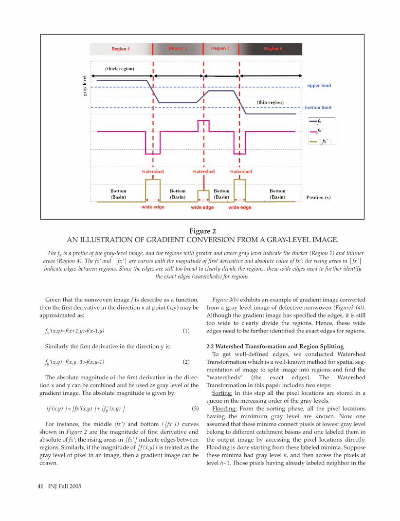
As previously mentioned, the AECvalue is an important factor, which influ-ences the result of defect inspection, so itshould be defined carefully. Suppose thestandard nonwoven is a fabric withoutdefect, thus the AEC value can be takenwhile the Def.% of standard nonwoven iszero. Figure 9 plots the relationshipbetween Def.% of standard nonwovensand AEC, which shows the Def.% decreas-es while the AEC increases. The Def.% isalmost zero when AEC reaches 3 in allsamples, which indicates that n=3 is agood selection for AEC value for defectinspection.

This process is illustrated below. The G(180.5) and σ (7.6) were evaluated from thestandard nonwoven of Sample A (see Table3) and were used to determined its Def.%

with given AEC value. Figure 10 displays the defect bound-aries in standard nonwoven of Sample A with various AECvalues and shows the Def.% is zero at AEC=3. Next, the defec-tive nonwoven of Sample A will be inspected by the criterionof AEC=3, G = 180.5 and σ = 7.6 according to the Eq.(7) andEq.(8). In another word, if the gth of defective nonwoven isout of the normal range between 157.7 (G -AEC*σ and 203.3(G +AEC*σ), the region will be treated as a defect. Figure 11reveals the defects that are explicitly delimited in the imagesof defective nonwoven by the NDDM method. The red and

47 INJ Fall 2005

Table 4THE DEF.% OF DEFECTIVE NONWOVENS

WITH VARIOUS IMAGE SIZES100*100 200*200 400*400

Sample A 57.9% 56.3% 54.1%Sample B 27.0% 23.5% 23.0%Sample C 44.7% 41.7% 39.0%

SAMPLE A

SAMPLE B

SAMPLE C

Figure 8THE STANDARD (LEFT) AND DEFECTIVE (RIGHT)

NONWOVENS

lai layout 10/10/05 2:15 PM Page 9

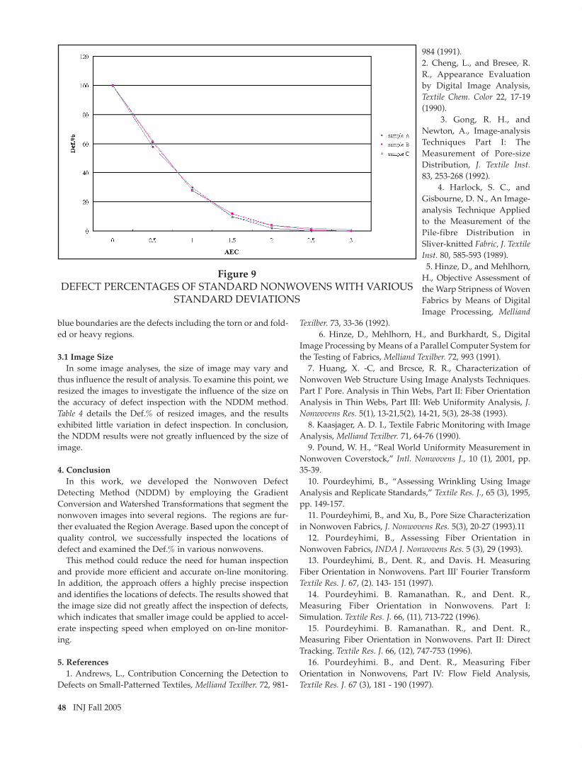
blue boundaries are the defects including the torn or and fold-ed or heavy regions.

3.1 Image SizeIn some image analyses, the size of image may vary and

thus influence the result of analysis. To examine this point, weresized the images to investigate the influence of the size onthe accuracy of defect inspection with the NDDM method.Table 4 details the Def.% of resized images, and the resultsexhibited little variation in defect inspection. In conclusion,the NDDM results were not greatly influenced by the size ofimage.

4. ConclusionIn this work, we developed the Nonwoven Defect

Detecting Method (NDDM) by employing the GradientConversion and Watershed Transformations that segment thenonwoven images into several regions. The regions are fur-ther evaluated the Region Average. Based upon the concept ofquality control, we successfully inspected the locations ofdefect and examined the Def.% in various nonwovens.

This method could reduce the need for human inspectionand provide more efficient and accurate on-line monitoring.In addition, the approach offers a highly precise inspectionand identifies the locations of defects. The results showed thatthe image size did not greatly affect the inspection of defects,which indicates that smaller image could be applied to accel-erate inspecting speed when employed on on-line monitor-ing.

5. References1. Andrews, L., Contribution Concerning the Detection to

Defects on Small-Patterned Textiles, Melliand Texilber. 72, 981-

984 (1991).2. Cheng, L., and Bresee, R.R., Appearance Evaluationby Digital Image Analysis,Textile Chem. Color 22, 17-19(1990).

3. Gong, R. H., andNewton, A., Image-analysisTechniques Part I: TheMeasurement of Pore-sizeDistribution, J. Textile Inst.83, 253-268 (1992).

4. Harlock, S. C., andGisbourne, D. N., An Image-analysis Technique Appliedto the Measurement of thePile-fibre Distribution inSliver-knitted Fabric, J. TextileInst. 80, 585-593 (1989).5. Hinze, D., and Mehlhorn,

H., Objective Assessment ofthe Warp Stripness of WovenFabrics by Means of DigitalImage Processing, Melliand

Texilber. 73, 33-36 (1992).6. Hinze, D., Mehlhorn, H., and Burkhardt, S., Digital

Image Processing by Means of a Parallel Computer System forthe Testing of Fabrics, Melliand Texilber. 72, 993 (1991).

7. Huang, X. -C, and Brcsce, R. R., Characterization ofNonwoven Web Structure Using Image Analysts Techniques.Part I' Pore. Analysis in Thin Webs, Part II: Fiber OrientationAnalysis in Thin Webs, Part III: Web Uniformity Analysis, J.Nonwovens Res. 5(1), 13-21,5(2), 14-21, 5(3), 28-38 (1993).

8. Kaasjager, A. D. I., Textile Fabric Monitoring with ImageAnalysis, Melliand Texilber. 71, 64-76 (1990).

9. Pound, W. H., “Real World Uniformity Measurement inNonwoven Coverstock,” Intl. Nonwovens J., 10 (1), 2001, pp.35-39.

10. Pourdeyhimi, B., “Assessing Wrinkling Using ImageAnalysis and Replicate Standards,” Textile Res. J., 65 (3), 1995,pp. 149-157.

11. Pourdeyhimi, B., and Xu, B., Pore Size Characterizationin Nonwoven Fabrics, J. Nonwovens Res. 5(3), 20-27 (1993).11

12. Pourdeyhimi, B., Assessing Fiber Orientation inNonwoven Fabrics, INDA J. Nonwovens Res. 5 (3), 29 (1993).

13. Pourdeyhimi, B., Dent. R., and Davis. H. MeasuringFiber Orientation in Nonwovens. Part III' Fourier TransformTextile Res. J. 67, (2). 143- 151 (1997).

14. Pourdeyhimi. B. Ramanathan. R., and Dent. R.,Measuring Fiber Orientation in Nonwovens. Part I:Simulation. Textile Res. J. 66, (11), 713-722 (1996).

15. Pourdeyhimi. B. Ramanathan. R., and Dent. R.,Measuring Fiber Orientation in Nonwovens. Part II: DirectTracking. Textile Res. J. 66, (12), 747-753 (1996).

16. Pourdeyhimi. B., and Dent. R., Measuring FiberOrientation in Nonwovens, Part IV: Flow Field Analysis,Textile Res. J. 67 (3), 181 - 190 (1997).

48 INJ Fall 2005

Figure 9DEFECT PERCENTAGES OF STANDARD NONWOVENS WITH VARIOUS

STANDARD DEVIATIONS

lai layout 10/10/05 2:15 PM Page 10

17. Pourdeyhimi. B., and Dent. R., Measuring FiberOrientation in Nonwovens, Part V: Real Web, Textile Res. J.69(3), 185- 192(1997).

18. Pro Schicktanz, K., Practical Experience with AutomaticCloth Inspection by the Laser-scan System, Melliand Texilber.71, 786-789 (1990).

19. Rajeev Chhabra, Scientist, “Nonwoven Uniformity —Measurements Using Image Analysis” INJ, spring, 2003, pp.

43-50.20. Robson, D., Weedall, P. J., and Itarwood, R. J., Cuticular

Scale Measurements Using Image Analysis Techniques, TextileRes. J. 59, 713-717 (1989).

21. Rosler, U., Defect Detection of Fabrics by ImageProcessing. Melliand Texilber. 73, 635-636 (1992).

22. Sobus, J., Pourdeyhimi, B., Gerde, J., and Ulcay, Y.,Assessing Changes in Texture Periodicity Due to Appearance

49 INJ Fall 2005

AEC=0.5 AEC=1.0

AEC=1.5 AEC=2.0

AEC=2.5 AEC=3.0

Figure 10DEFECT BOUNDARIES OF STANDARD NONWOVEN (SAM-

PLE A) UNDER VARIOUS AEC

lai layout 10/10/05 2:15 PM Page 11

Loss in Carpet: Gray Level Co-occurrence Analysis, TextileRes. J. 61,557-567 (1991).

23. Taylor, R. A., Estimating the Size of Cotton Trash withVideo Images, Textile Res. J. 60, 185-193 (1990).

24. Watanabe, A., Kurosaki, S. -N., and Konda, F., Analysisof Blend Irregularity in Yarns Using Image Processing, Part 1:Fundamental Investigation of Model Yarns, Textile Res. J. 62,690-696 (1992).

25. Wood, E. J., Applying Fourier and Associated forms toPattern Characterization in Textiles, Res. J. 60, 212-220 (1990).

26. Wu, Y., Pourdcyhimi, B. Spivak, S. M., and Hollics, N. R.

S., Instrumental Techniques to Quantify Textural andAppearance Changes in Carpet, Part IV: Colorimetric ImageAnalysis, Textile Res. J. 60, 673-687 (1990).

27. Wu, Y., Pourdeyhimi, B., and Spivak, S. M., TextureEvaluation of Carpets Using Image Analysis, Textile Res. J. 61,407-419 (1991).

28. Xu, B., Pourdeyhimi, B., and Sobus, J., CharacterizingFiber Crimp Using Image Analysis: Definitions, Algorithms,and Techniques, Textile Res. J. 62, 73-80 (1992). — INJ

50 INJ Fall 2005

SAMPLE ATHIN DEFECT AREA (%) 18.1THICK DEFECT AREA(%) 11.6TOTAL DEFECT AREA 29.7

SAMPLE BTHIN DEFECT AREA (%) 18.1THICK DEFECT AREA(%) 11.6TOTAL DEFECT AREA(%) 29.7

SAMPLE CTHIN DEFECT AREA(%) 31.2THICK DEFECT AREA(%) 0TOTAL DEFECT AREA(%) 31.2

Figure 11DEFECTIVE AREA AND BOUNDARIES OF DEFECTIVE NONWOVENS

lai layout 10/10/05 2:15 PM Page 12

The International Nonwovens Journal is brought to you fromAssociations from around the world. This critical technicalpublication is provided as a complimentary service to the

membership of the Associations that providedthe funding and hard work.

PUBLISHER

INDA, ASSOCIATION OF THE NONWOVEN FABRICS INDUSTRYRORY HOLMES

PRESIDENTP.O. BOX 1288, CARY, NC 27511

www.inda.org

SPONSOR

TAPPI, TECHNICAL ASSOCIATION OF THE PULP AND PAPER INDUSTRYWAYNE H. GROSS

EXECUTIVE DIRECTOR/COOP.O. BOX 105113

ATLANTA, GA 30348-5113www.tappi.org