Embed Size (px)
Citation preview

An idealised fluid model of Numerical Weather
Prediction: dynamics and data assimilation
Thomas Kent
Submitted in accordance with the requirements for the degree of Doctor
of Philosophy
University of Leeds
Department of Applied Mathematics
December 2016

ii

iii
Declaration
The candidate confirms that the work submitted is his own and that appropriate credit has
been given where reference has been made to the work of others.
This copy has been supplied on the understanding that it is copyright material and that no
quotation from the thesis may be published without proper acknowledgement.
©2016 The University of Leeds and Thomas Kent
The right of Thomas Kent to be identified as Author of this work has been asserted by
him in accordance with the Copyright, Designs and Patents Act 1988.

iv

v
Acknowledgements
I would like to express my gratitude to number of people who have supported me working
towards this thesis during my time in Leeds. First, I thank Onno Bokhove for his support,
guidance, and patience over the last three and half years. His enthusiasm for this work
and all things scientific has been inspiring. Thanks also to Steve Tobias for always
contributing the time and assistance when needed, despite heading the department for
these years. I would also like to thank my advisor from the Met Office, Gordon Inverarity,
for numerous helpful discussions and support during my visits to Exeter and via Skype in
these last months. His input has been crucial in this project and I have benefited hugely
from his expertise in data assimilation and numerical weather prediction. And to all three,
thank you for proof-reading this work.
I would also like to mention Neill Bowler and Mike Cullen at the Met Office for their input
over the years, and the ‘Data Assimilation Methods’ group for welcoming me during my
time in Exeter. And to Keith Ngan, who proposed and secured funding for the project
before leaving for Hong Kong. This project would not have been possible without the
generous financial support of the Engineering and Physical Sciences Research Council
and the Met Office.
Being the only Data Assimilator in Leeds, this research has felt at times a slow and solitary
journey. But the support and interest shown by the DA community has made a huge
difference and it has been a pleasure to participate in stimulating meetings in the UK and
abroad. Particular thanks go to the group at Reading University. And finally, to friends
and family, for getting me here in the first place, and their continual encouragement and
support in all things.

vi

vii
AbstractThe dynamics of the atmosphere span a tremendous range of spatial and temporal scales
which presents a great challenge to those who seek to forecast the weather. To aid
understanding of and facilitate research into such complex physical systems, ‘idealised’
models can be developed that embody essential characteristics of these systems. This
thesis concerns the development of an idealised fluid model of convective-scale Numerical
Weather Prediction (NWP) and its use in inexpensive data assimilation (DA) experiments.
The model modifies the rotating shallow water equations to include some simplified
dynamics of cumulus convection and associated precipitation, extending the model of
Wursch and Craig [2014]. Despite the non-trivial modifications to the parent equations, it
is shown that the model remains hyperbolic in character and can be integrated accordingly
using a discontinuous Galerkin finite element method for nonconservative hyperbolic
systems of partial differential equations. Combined with methods to ensure well-
balancedness and non-negativity, the resulting numerical solver is novel, efficient, and
robust. Classical numerical experiments in shallow water theory, based on the Rossby
geostrophic adjustment problem and non-rotating flow over topography, elucidate the
model’s distinctive dynamics, including the disruption of large-scale balanced flows
and other features of convecting and precipitating weather systems. When using such
intermediate-complexity models for DA research, it is important to justify their relevance
in the context of NWP. A well–tuned observing system and filter configuration is achieved
using the ensemble Kalman filter that adequately estimates the forecast error and has
an average observational influence similar to NWP. Furthermore, the resulting error-
doubling time statistics reflect those of convection-permitting models in a cycled forecast–
assimilation system, further demonstrating the model’s suitability for conducting DA
experiments in the presence of convection and precipitation. In particular, the numerical
solver arising from this research provides a useful tool to the community and facilitates
other studies in the field of convective-scale DA research.

viii
ix
Contents
Declaration . . . . . . . . . . . . . . . . . . . . . . . . . . . . . . . . . . . . iii
Acknowledgements . . . . . . . . . . . . . . . . . . . . . . . . . . . . . . . . v
Abstract . . . . . . . . . . . . . . . . . . . . . . . . . . . . . . . . . . . . . . vii
Contents . . . . . . . . . . . . . . . . . . . . . . . . . . . . . . . . . . . . . . ix
List of figures . . . . . . . . . . . . . . . . . . . . . . . . . . . . . . . . . . . xiv
List of tables . . . . . . . . . . . . . . . . . . . . . . . . . . . . . . . . . . . . xxi
1 Introduction 1
1.1 Background and motivation . . . . . . . . . . . . . . . . . . . . . . . . . 1
1.2 Aims . . . . . . . . . . . . . . . . . . . . . . . . . . . . . . . . . . . . . 10
1.3 Thesis outline . . . . . . . . . . . . . . . . . . . . . . . . . . . . . . . . 11
2 An idealised fluid model of NWP 13
2.1 Shallow water modelling . . . . . . . . . . . . . . . . . . . . . . . . . . 14
2.1.1 The classical equations . . . . . . . . . . . . . . . . . . . . . . . 15
2.2 Modified Shallow Water . . . . . . . . . . . . . . . . . . . . . . . . . . 16
2.3 Summary . . . . . . . . . . . . . . . . . . . . . . . . . . . . . . . . . . 24

x CONTENTS
3 Numerics 25
3.1 1D DGFEM for hyperbolic conservation laws . . . . . . . . . . . . . . . 26
3.1.1 Computational mesh . . . . . . . . . . . . . . . . . . . . . . . . 26
3.1.2 Weak formulation . . . . . . . . . . . . . . . . . . . . . . . . . . 27
3.1.3 Space-DG0 discretisation . . . . . . . . . . . . . . . . . . . . . . 30
3.1.4 Boundary conditions and ghost elements . . . . . . . . . . . . . 30
3.2 1D DGFEM for non-conservative hyperbolic PDEs . . . . . . . . . . . . 32
3.2.1 DLM theory . . . . . . . . . . . . . . . . . . . . . . . . . . . . 33
3.2.2 Weak formulation . . . . . . . . . . . . . . . . . . . . . . . . . . 34
3.2.3 Space-DG0 discretisation . . . . . . . . . . . . . . . . . . . . . . 35
3.3 SWEs: issues with well-balancedness at DG0 . . . . . . . . . . . . . . . 36
3.4 Numerical formulation: modRSW . . . . . . . . . . . . . . . . . . . . . 40
3.4.1 Approach: a mixed NCP-Audusse scheme . . . . . . . . . . . . . 40
3.4.2 Discretising the topographic source term . . . . . . . . . . . . . 41
3.4.3 NCP flux: derivation . . . . . . . . . . . . . . . . . . . . . . . . 42
3.4.4 Outline: mixed NCP-Audusse scheme . . . . . . . . . . . . . . . 49
4 Dynamics 51
4.1 Numerical experiments . . . . . . . . . . . . . . . . . . . . . . . . . . . 52
4.1.1 Rossby adjustment scenario . . . . . . . . . . . . . . . . . . . . 53
4.1.2 Flow over topography . . . . . . . . . . . . . . . . . . . . . . . 61
4.2 Summary . . . . . . . . . . . . . . . . . . . . . . . . . . . . . . . . . . 69

CONTENTS xi
5 Data assimilation and ensembles: background, theory, and practice 71
5.1 Overview of the classical DA problem . . . . . . . . . . . . . . . . . . . 72
5.2 Kalman Filtering . . . . . . . . . . . . . . . . . . . . . . . . . . . . . . 79
5.2.1 The forecast step . . . . . . . . . . . . . . . . . . . . . . . . . . 80
5.2.2 The analysis step . . . . . . . . . . . . . . . . . . . . . . . . . . 82
5.2.3 Summary . . . . . . . . . . . . . . . . . . . . . . . . . . . . . . 84
5.3 The Ensemble Kalman Filter . . . . . . . . . . . . . . . . . . . . . . . . 86
5.3.1 Basic equations . . . . . . . . . . . . . . . . . . . . . . . . . . . 87
5.3.2 The stochastic filter: treatment of observations . . . . . . . . . . 89
5.3.3 Matrix formulation . . . . . . . . . . . . . . . . . . . . . . . . . 93
5.3.4 Summary . . . . . . . . . . . . . . . . . . . . . . . . . . . . . . 95
5.4 Other filters . . . . . . . . . . . . . . . . . . . . . . . . . . . . . . . . . 97
5.4.1 Deterministic filters . . . . . . . . . . . . . . . . . . . . . . . . . 97
5.4.2 Ensemble transform filters . . . . . . . . . . . . . . . . . . . . . 98
5.4.3 Nonlinear filters . . . . . . . . . . . . . . . . . . . . . . . . . . 99
5.5 Issues in ensemble-based Kalman filtering . . . . . . . . . . . . . . . . . 99
5.5.1 The rank problem and ensemble subspace . . . . . . . . . . . . . 100
5.5.2 Maintaining ensemble spread: the need for inflation . . . . . . . . 101
5.5.3 Spurious correlations: the need for localisation . . . . . . . . . . 104
5.6 Interpreting an ensemble-based forecast-assimilation system . . . . . . . 108
5.6.1 Error vs. spread . . . . . . . . . . . . . . . . . . . . . . . . . . . 108

xii CONTENTS
5.6.2 Observation influence diagnostic . . . . . . . . . . . . . . . . . . 108
5.6.3 Continuous Ranked Probability Score . . . . . . . . . . . . . . . 110
5.6.4 Error-growth rates . . . . . . . . . . . . . . . . . . . . . . . . . 112
6 Idealised DA experiments 115
6.1 Twin model environment . . . . . . . . . . . . . . . . . . . . . . . . . . 116
6.1.1 Setting up an idealised forecast–assimilation system . . . . . . . 117
6.1.2 Tuning a forecast–assimilation system . . . . . . . . . . . . . . . 124
6.2 Results . . . . . . . . . . . . . . . . . . . . . . . . . . . . . . . . . . . . 126
6.2.1 The need for additive inflation . . . . . . . . . . . . . . . . . . . 126
6.2.2 Summarising the tuning process . . . . . . . . . . . . . . . . . . 131
6.2.3 Experiment: ∆y = 40, γm = 1.01, Lloc =∞ . . . . . . . . . . . 139
6.3 Synopsis . . . . . . . . . . . . . . . . . . . . . . . . . . . . . . . . . . . 147
7 Conclusion 151
7.1 Summary . . . . . . . . . . . . . . . . . . . . . . . . . . . . . . . . . . 151
7.2 Aims revisited . . . . . . . . . . . . . . . . . . . . . . . . . . . . . . . . 155
7.3 Future work: plans and ideas . . . . . . . . . . . . . . . . . . . . . . . . 157
Appendix 161
A The model of Wursch and Craig [2014] . . . . . . . . . . . . . . . . . . 161
B Non-negativity preserving numerics . . . . . . . . . . . . . . . . . . . . 163
C Well-balancedness: DG1 proof . . . . . . . . . . . . . . . . . . . . . . . 174

CONTENTS xiii
Bibliography 179

xiv List of figures
xv
List of figures
2.1 Schematic of the pressure term P (h; b) in (2.3): the modified pressure
p(Hc−b) = 12g(Hc−b)2 above the thresholdHc is lower than the standard
pressure p(h) = 12gh2, thus forcing the fluid to rise where h+ b > Hc. . . 18
3.1 The computational mesh Th (3.3) is extended to include a set of ghost
elements K0 and KNel+1 at the boundaries (see section 3.1.4). Central
to the DGFEM schemes are the fluxes numerical F through the nodes,
introduced in section 3.1.2. . . . . . . . . . . . . . . . . . . . . . . . . . 27
4.1 Time evolution of the height profile h(x, t) for the case I (left), II (middle),
III (right). Non-dimensional simulation details: Ro = 0.1,Fr = 1, Nel =
250; (Hc, Hr) = (1.01, 1.05); (α, β, c20) = (10, 0.1, 0.81). . . . . . . . . . 53
4.2 Time evolution of the height profile h(x, t) for case I only: Nel = 250
(dotted), Nel = 500 (dashed), Nel = 1000 (solid). The L∞ norm for
Nel = 250 and Nel = 500 is computed at each time with respect to the
Nel = 1000 simulation (denoted L∞250 and L∞500 respectively), and verifies
convergence of the scheme. Doubling the number of elements leads to an
error reduction of factor two, as expected for a DGO scheme. . . . . . . . 55

xvi LIST OF FIGURES
4.3 Hovmoller plots for the Rossby adjustment process with initial transverse
jet: case I (left), II (middle), and III (right). From top to bottom:
h(x, t), u(x, t), v(x, t), and r(x, t). Non-dimensional simulation details:
same as figure 4.1. . . . . . . . . . . . . . . . . . . . . . . . . . . . . . 56
4.4 Evolution of h and r for the Rossby adjustment process with initial
transverse jet: case I (left), II (middle), and III (right). Top row:
Hovmoller plots for h. Subsequent rows: profiles of h (black line; left
axis) and r (blue line; right axis) at different times denoted by the dashed
lines in the top row. Non-dimensional simulation details: same as figure
4.1. . . . . . . . . . . . . . . . . . . . . . . . . . . . . . . . . . . . . . 58
4.5 Hovmoller plots for the Rossby adjustment process with initial transverse
jet, highlighting the conditions for the production of rain: case III. From
left to right: h > Hr,−∂xu > 0, and r(x, t). Non-dimensional simulation
details: same as figure 4.1. . . . . . . . . . . . . . . . . . . . . . . . . . 59
4.6 Top row: Hovmoller diagram plotting the evolution of the departure from
geostrophic balance g∂xh−fv: light (deep) shading denotes regions close
to (far from) geostrophic balance. Subsequent rows: profiles of fv (red)
and g∂xh (black) at different times denoted by the dashed lines in the top
figure. For case I (left), II (middle), and III (right). Non-dimensional
simulation details: same as figure 4.1. . . . . . . . . . . . . . . . . . . . 60
4.7 Flow over topography (bc = 0.5, a = 0.05, and xp = 0.1): profiles of
h + b, b (black; left y-axis), exact steady-state solution for the SWEs
(red dashed; as derived in section 4.1.2) and rain r (blue; right y-
axis) at different times: case I (left), II (middle), and III (right). The
dotted lines denote the threshold heights Hc < Hr. Non-dimensional
simulation details: Fr = 2; Ro = ∞;Nel = 1000; (Hc, Hr) =
(1.2, 1.25); (α, β, c20) = (10, 0.1, 0.081). . . . . . . . . . . . . . . . . . . 63

LIST OF FIGURES xvii
4.8 Hovmoller plots for flow over topography (Fr = 2), highlighting the
conditions for the production and subsequent evolution of rain: case III.
From left to right: h + b, −∂xu, and r. Non-dimensional simulation
details: same as figure 4.7. . . . . . . . . . . . . . . . . . . . . . . . . . 64
4.9 Same as figure 4.7 but with two orographic ridges: bc = 0.4, a = 0.05,
and (xp1 , xp2) = (0.0875, 0.2625). Non-dimensional simulation details:
same as figure 4.7. . . . . . . . . . . . . . . . . . . . . . . . . . . . . . 65
4.10 Same as figure 4.8 but with two orographic ridges. Non-dimensional
simulation details: same as figure 4.7. . . . . . . . . . . . . . . . . . . . 66
5.1 A schematic diagram illustrating the general formulation of the KF. The
filtering technique starts with some given prior information and then
continues in cycles with the availability of observations. . . . . . . . . . . 85
5.2 A schematic diagram illustrating the general formulation of the EnKF.
The EnKF forecast and update equations with perturbed observations are
structurally identical to those of the traditional and extended KF. . . . . . 96
5.3 Example Gaspari-Cohn functions % for different length-scales Lloc as a
function of distance x. Here, x is the number of equally-spaced grid
points away from the observation location at x = 0. Lloc =∞ implies no
localisation (cyan line); the smaller Lloc, the tighter the localisation. The
number of grid points relates to the experiments in chapter 6. . . . . . . . 107

xviii LIST OF FIGURES
6.1 Snapshot of model variables h (top), u (middle), and r (bottom) from
(a) the forecast model and (b) the nature run. The forecast trajectory
is smoother and exhibits ‘under-resolved’ convection and precipitation
while the nature run has sharper ‘resolved’ features and is a proxy for the
truth. The thick black line in the top panels is the topography (eq. 6.1),
the red dotted lines are the threshold heights. . . . . . . . . . . . . . . . . 118
6.2 Ensemble spread (solid) vs. RMSE of the ensemble mean (dashed): from
top to bottom h, u, r. Without additive inflation, insufficient spread leads
rapidly to filter divergence; with additive inflation, the ensemble spread
is comparable to the RMSE of the ensemble mean, thus preventing filter
divergence. The time-averaged values are given in the top-left corner. . . 128
6.3 Ensemble trajectories (blue) and their mean (red for forecast; cyan for analysis),
pseudo-observations (green circles with corresponding error bars), and nature
run (green solid line) after 36 hours/cycles. Left column: forecast ensemble (i.e.,
prior distribution, before assimilation); right column: analysis ensemble (i.e.,
posterior distribution, after assimilation). . . . . . . . . . . . . . . . . . . . 130
6.4 Average RMS error and spread: for different combinations of
multiplicative inflation γm (x-axis) and localisation lengthscales Lloc (y-
axis); additive inflation γa = 0.45 and observation density ∆y = 20 (so
p = 30). Top - error; bottom - spread; left - forecast; right - analysis.
The experiment that produces the lowest analysis error is in bold, namely
Lloc = ∞, γm = 1.01. ‘NaN’ denotes an experiment that crashed before
48 hours. . . . . . . . . . . . . . . . . . . . . . . . . . . . . . . . . . . 133
6.5 Same as figure 6.4 but with ∆y = 40 (i.e., p = 15). Note that the colour
bar is slighty different to that in figure 6.4. . . . . . . . . . . . . . . . . . 134

LIST OF FIGURES xix
6.6 Continuous Ranked Probability Score (5.6.3): for different combinations
of multiplicative inflation γm (x-axis) and localisation lengthscales Lloc
(y-axis); additive inflation γa = 0.45 and observation density (a) ∆y =
20 and (b) ∆y = 40. Left - forecast; right - analysis. . . . . . . . . . . . 135
6.7 Averaged Observational Influence Diagnostic (equation (5.77) in section
5.6.2): for different combinations of multiplicative inflation γm (x-axis)
and localisation lengthscales Lloc (y-axis); additive inflation γa = 0.45
and observation density (a) ∆y = 20 and (b) ∆y = 40. The experiment
with the largest observational influence is in bold. In general, the
influence increases with γm and localisation. . . . . . . . . . . . . . . . . 137
6.8 Error vs. spread measure and CRPS for the ∆y = 40, γm = 1.01, Lloc =
∞ experiment. (a) The ensemble spread is comparable to the RMSE of
the ensemble mean for both the forecast (red) and analysis (blue). (b) The
assimilation update improves the reliability of the ensemble. From top to
bottom: h, u, r. Time-averaged values are given in the top-left corner. . . 139
6.9 Time series of the observational influence diagnostic: the overall
influence (thick black line) fluctuates between 10–25% with an average of
15.4%. Coloured lines (see legend) indicate the influence of the individual
variables and sum to the overall influence. . . . . . . . . . . . . . . . . . 141
6.10 Ensemble trajectories (blue) and their mean (red for forecast; cyan for
analysis), pseudo-observations (green circles with corresponding error
bars), and nature run (green solid line) after 36 hours/cycles. Left column:
forecast ensemble (i.e., prior distribution, before assimilation); right
column: analysis ensemble (i.e., posterior distribution, after assimilation) 142

xx LIST OF FIGURES
6.11 Left column: error (dashed) and spread (solid) as a function of x
at T=36. Both are of a similar magnitude and larger in regions of
convection/precipitation (cf. figure 6.10), where the flow is highly
nonlinear. Domain-averaged values are given in the top-left corner. Right
column: the difference between the error and spread. Positive (negative)
values indicate under- (over-) spread. . . . . . . . . . . . . . . . . . . . . 144
6.12 CRPS as a function of x at T=36: forecast (red) and analysis (blue)
ensemble. The ensembles are less reliable (higher CRPS values) in
regions of convection and precipitation. Domain-averaged values are
given in the top-right corner. . . . . . . . . . . . . . . . . . . . . . . . . 145
6.13 Histograms of the error-doubling times (5.6.4) for 640 24-hour forecasts
initialised using analysis increments from the idealised forecast-
assimilation system. From top to bottom: h, u, r. The average doubling
time in convection-permitting NWP models is around 4 hours. . . . . . . 146
6.14 Facets of localisation: taper functions, a localising matrix, and the effect
on correlation matrices. Top left: Gaspari-Cohn taper functions %(x) for
a given cut-off length-scale Lloc. Top right: the 3 × 3 block localisation
matrix ρ ∈ Rn×n computed from % with Lloc = 80. Bottom left: a
correlation matrix after T=36 cycles from the experiment with ∆y = 40,
γm = 1.01, Lloc = ∞. Notice the strength of off-diagonal correlations.
Bottom right: the same correlation matrix localised using the above ρ
with Lloc = 80. This suggests that applying localisation in this setting
suppresses true covariances, thereby degrading the analysis. . . . . . . . . 148
B.1 Parabolic bowl problem at times t = 400, 800, 1200, 1600: blue - bottom
topography b, green - exact solution h+ b , red - numerical solution h+ b.
The computational domain is [−5000, 5000] with 1000 uniform cells. . . . 173

xxi
List of tables
6.1 Parameters used in the idealised forecast-assimilation experiments. . . . . 132

xxii LIST OF TABLES

1
Chapter 1
Introduction
“The most important task of theoretical meteorology will ultimately be
to take a picture of the condition of the atmosphere as a starting point for
constructing future states.”1
1.1 Background and motivation
Since Aristotle’s Meteorologica attempted to describe and explain properties of the
atmosphere over two millennia ago, humankind has been both fascinated and perplexed
by the weather. In the centuries since, societies have sought greater understanding of
this complex natural phenomenon and recognised its benefit to society, with the ultimate
ambition of making accurate predictions of the future state of the atmosphere. However, it
wasn’t until the second half of the 19th century that significant progress was made towards
achieving this ambition. In 1854, ‘weather forecasting’ became more formalised, with
the creation of the Meteorological Board of Trade in Britain, considered the world’s first
national weather service and a precursor of today’s Met Office in the United Kingdom.
This new organisation was headed by Robert FitzRoy, who gained insight and interest1From Bjerknes [1904] seminal paper, elucidating ‘The Problem of Weather Prediction’.

2 Chapter 1. Introduction
in meteorology while in the navy and set about expanding weather reports and logging
observation data from land and sea. Using the network of observations, FitzRoy plotted
the variable values, such as surface pressure, on a map to give a rough picture of the
state of the atmosphere, and the synoptic chart was born. In the same year, an eminent
astronomer in France, Urbain Le Verrier, turned his mind and hand to meteorology at the
behest of Louis-Napoleon III. Le Verrier had used Newtonian mechanics to predict the
location of a hitherto unobserved planet with startling accuracy – surely the same could
be applied to weather forecasting? Le Verrier also used reports and data from weather
stations to make inferences on the direction and speed of weather systems, particularly
storms. However, unlike astronomy, where Newton’s laws were applied with great
success, there was a distinct lack of physical laws and equations (apart from empirical
rules) in these early weather forecasts, which were formed of hand–drawn charts and
comprised ‘subjective analysis’ only.
In 1904, after years ruminating the fundamental problem of weather forecasting,
Norwegian scientist Vilhelm Bjerknes published a paper framing meteorology from a
hydrodynamic perspective and formulating the problem in terms of the natural laws
of physics [Bjerknes, 1904]. He posited that the future state of the atmosphere is, in
principle, completely determined by the primitive equtions of motion, mass, state, and
energy, together with its known initial state and boundary conditions, given two necessary
and sufficient conditions:
1. the state of the atmosphere is known with sufficient accuracy at a given time;
2. the laws that govern how one state of the atmosphere develops from another are
known with sufficient accuracy.
However, Bjerknes recognised that the governing equations for the whole atmosphere
were far too complex to be solved exactly – a mathemetical problem that remains unsolved
today. Instead, he suggested that the problem should be simplified and solved numerically

Chapter 1. Introduction 3
in discrete subdomains and time intervals. It is striking how prescient Bjerknes’ work and
ideas remain to this day and his seminal paper is widely regarded as the dawn of modern
weather forecasting and numerical weather prediction.
Richardson [1922] came up with a scheme for integrating the equations of motion and
imagined huge “forecast factories” computing the motion of the atmosphere:
“After so much hard reasoning, may one play with fantasy? Imagine a
large hall like a theatre, except that the circles and galleries go right round
through the space usually occupied by the stage. The walls of this chamber
are painted to form a map of the globe. The ceiling represents the north polar
regions, England is in the gallery, the tropics in the upper circle, Australia on
the dress circle and the Antarctic in the pit. A myriad computers are at work
upon the weather of the part of the map where each sits, but each computer
attends only to one equation or part of an equation”.
Considered the first attempt at numerical weather prediction (NWP), Richardson
produced a forecast for surface pressure tendency in Germany, numerically integrating the
equations of motion by hand. The solution was alarmingly inaccurate however, predicting
a pressure tendency of 146hPa over six hours (for comparison, the highest and lowest
recorded surface pressure in the UK is 1055hPa and 925hPa respectively). The equations
Richardson solved were valid, but the forecast failed for two reasons: first, the discrete
time interval used for integrating forward in time was too large, violating the as yet
undiscovered Courant-Friedrichs-Lewy time step criterion for numerical stability; second,
Bjerknes’ first condition was not satisfied – noise in the initial conditions destroyed the
solution [Kalnay, 2003].
Nonetheless, Richardson’s failed attempt was ingenious and his ideas of fantasy would
become reality, albeit with far less dramatic imagery. The dawn of computation prompted
massive developments in NWP. In ‘Dynamical forecasting by numerical process’, Jule
4 Chapter 1. Introduction
Charney recognised Richardson’s efforts, commenting: “that the actual forecast used to
test his method was unsuccessful was in no way a measure of the value of his work”
[Charney, 1951]. Charney, along with others in the USA and Sweden, pioneered the use
of modern computers in weather forecasting and witnessed the beginning of operational
(real–time) NWP in the 1950s, which used ‘objective analysis’ to incorporate observations
in the initial conditions. Typically, there are far fewer observations than degrees of
freedom of a forecast model, and observations are spatially incomplete. Thus, the
initialisation problem is ill–posed and cannot be satisfactorily solved by simply inserting
observational values alone. Some other information is required to ‘take a full picture
of the condition of the atmosphere’, in Bjerknes’ words. The ‘objective analysis’ of
Gilchrist and Cressman [1954] combines observations with some prior estimate of the
system (from, e.g., a prior forecast or climatology), which regularises the problem and
provides an improved estimate of the state.
Around the same time as Bjerknes espoused his rational approach to weather forecasting,
the French mathematician Henri Poincare published ‘Science and Method’, which would
have similarly significant repercussions in the field of weather forecasting and beyond
[Poincare, 1914]. Determinism, the notion that knowledge of the current state of a
mechanical system completely determines its future (and past), is the foundation of
classical mechanics and had dominated scientific thinking since Newton’s Principia
Mathematica was published in the 17th century. Poincare postulated that even if the
laws of nature were known exactly, the current state of nature can only ever be known
approximately. Moreover, this approximation, when applied to the laws of nature, may
produce a future state that diverges enormously from the correct future state, especially
if those laws are nonlinear. This concept is manifest as chaos: “small differences in the
initial conditions produce very great ones in the final phenomena” [Poincare, 1914].
The atmosphere is an unstable, chaotic system that possesses myriad dynamical processes
over a range of temporal and spatial scales. Thus, small errors in the initial conditions will

Chapter 1. Introduction 5
grow to become large errors in the resulting forecast, and long–term prediction becomes
impossible. Chaos, error–growth, and atmospheric predictability were brought together
by Edward Lorenz, who confirmed that even if the forecast model is perfect, there is an
upper limit to weather predictability [Lorenz, 1963]. The implication for NWP is that
the models must go through a regular process of reinitialisation as observations become
available in time to restore information lost through error growth due to chaos.
Thus, despite the limitations of the component parts of NWP (imperfect models,
imperfect data) and the constraints on predictability owing to chaos, weather forecasting
remains possible, and indeed successful, due to the regular updates from observations.
Development continued apace towards the end of the 20th century as computational power
expanded greatly, allowing higher spatial resolution and more vertical layers in the model
grids. Furthermore, the advent of satellite data in the 1970s provided new sources of
observations and typically covered hitherto data–sparse geographical areas. This led
to a dramatic increase in forecast skill, highlighting the importance of observational
information in the NWP problem.
Today’s NWP models integrate the full primitive equations of motion, describing
atmospheric motions on many scales whilst parameterising unresolved processes at the
smaller scales as a function of the resolved state. As exemplified by Bjerknes, NWP can
be thought of as an initial value problem comprising a forecast model and suitable initial
conditions, with its accuracy depending critically on both, and which needs reinitialising
regularly to restore information lost through error growth. Data Assimilation (DA; see,
e.g., Kalnay [2003]) attempts to provide the optimal initial conditions for the forecast
model by estimating the state of the atmosphere and its uncertainty using a combination
of forecast and observational information (and taking into account their respective
uncertainties). As demonstrated in Richardson’s first attempt, a “sufficiently accurate”
initial state is crucial in such a highly nonlinear system with limited predictability and is
a key component of NWP. A great deal of attention is thus focussed on observing systems

6 Chapter 1. Introduction
and assimilation algorithms; this thesis concerns DA for an idealised mathematical model
of NWP.
Until recently, operational NWP models were running with a horizontal resolution larger
than the size of most convective disturbances, such as cumulus cloud formation, which
were accordingly parameterised. Despite the coarse resolution leaving many ‘subgrid’-
scale dynamical processes unresolved, there has been a great deal of success in weather
forecasting owing mainly to the dominance of large-scale dynamics in the atmosphere
[Cullen, 2006]. ‘Variational’ DA algorithms have successfully exploited this notion that
atmospheric dynamics in the extra-tropics are close to a balanced state (e.g., hydrostatic
and semi-/quasi-geostrophic balance), resulting in analysed states and forecasts that
remain likewise close to this balance [Bannister, 2010].
Increasing computational capability has led in recent years to the development of high-
resolution models at national meteorological centres in which some of the convective-
scale dynamics are explicitly (or at least partially) resolved (e.g., Done et al. [2004];
Baldauf et al. [2011]; Tang et al. [2013]). This so-called ‘grey-zone’, the range of
horizontal scales in which convection and cloud processes are being partly resolved
dynamically and partly by subgrid parameterisations, presents a considerable challenge to
the NWP and DA community [Hong and Dudhia, 2012]. Current regional NWP models
are running at a spatial gridsize on the order of 1km with future refinement inevitable,
and smaller-scale processes are known to interfere with DA algorithms based on the
aforesaid balance principles [Vetra-Carvalho et al., 2012]. As such, high-resolution NWP
benefits hugely from having its own DA system, rather than using a downscaled large-
scale analysis [Dow and Macpherson, 2013].
A crucial part of any DA scheme is the adequate estimation of errors associated with the
forecast, or ‘background’ estimate. Due to the size of the NWP problem, it is not possible
to explicitly calculate or store the full-dimensional error statistics which need modelling
accordingly. The error covariance modelling (Bannister [2008a,b]) required in variational

Chapter 1. Introduction 7
DA algorithms is often suboptimal for high-resolution DA owing to convective-scale
motions exhibiting larger error growth at smaller timescales. Motivated by the need
for flow-dependent errors and the simultaneous development of ensemble forecasting
systems, there is a general consensus (e.g., Zhang et al. [2004]; Bannister et al. [2011];
Ballard et al. [2012]; Schraff et al. [2016]) to move towards ensemble-based DA methods
(either purely ensemble-based or an ensemble-variational hybrid), which use a Monte-
Carlo sample (‘ensemble’) of forecast trajectories to estimate the error covariances.
To aid understanding of and facilitate research into such large and complex operational
forecast-assimilation systems, simplified models can be utilised that represent some
essential features of these systems yet are computationally inexpensive and easy
to implement. This allows one to investigate and optimise current and alternative
assimilation algorithms in a cleaner environment before making insights or considering
implementation in a full NWP model [Ehrendorfer, 2007]. By starting with simplified
models, and gradually increasing complexity, one can proceed inductively, and hopefully
avoid problems when many (potentially poorly understood) factors are introduced all at
once. It is often this approach that drives development and progress in DA, including
the aforementioned issues posed by high-resolution NWP, from research to operational
forecasting.
Perhaps the most famous ‘toy’ model in meteorology is Lorenz’s low-order convection
model (L63; Lorenz [1963]). Despite containing only three variables, this system of
ordinary differential equations (ODEs) describes idealised dissipative hydrodynamic flow
and exhibits high nonlinearity. The L63 model and its successors [Lorenz, 1986, 1996;
Lorenz and Emanuel, 1998; Lorenz, 2005] continue to be the basis for numerous DA
studies (e.g., Neef et al. [2006, 2009]; Subramanian et al. [2012]; Bowler et al. [2013];
Fairbairn et al. [2014]). They provide chaotic dynamics on a range of scales yet their
low dimensionality means that they are computationally cheap and easy to implement in
a data assimilation system.

8 Chapter 1. Introduction
Whilst being invaluable tools and offering dynamical phenomena of sufficient interest for
investigating DA algorithms, there is a vast gap between the complexity of such ODE
models and the primitive equation models of operational forecasting. Simplified fluid
models attempt to bridge this gap in the hierarchy of complexity. Shallow water models
capture interactions between waves and vortical motions in rotating stratified fluids and
have received much attention in DA research for the ocean and atmosphere (e.g., Zhu et al.
[1994]; Zagar et al. [2004]; Salman et al. [2006]; Stewart et al. [2013]). Continuing up
the hierarchy, idealised configurations of operational NWP models (e.g., Lange and Craig
[2014]) provide the closest representation of operational forecast–assimilation systems
with which to examine potential advances in performance of new schemes.
Arguably the best way, therefore, to approach convective–scale DA research is by using
idealised models that capture some fundamental features of convective–scale dynamics
that are relevant for high–resolution NWP. In this thesis, a modified shallow water model
(extending that of Wursch and Craig [2014]) is proposed for this purpose. It modifies
the shallow water equations (SWEs) to model some dynamics of cumulus convection,
including rapid ascent and descent of air, and the transport of moisture via a ‘rain mass
fraction’ variable r, and is intended primarily for use as a testbed for convective–scale DA
research.
Convective (cumulus) clouds are characterized by highly buoyant, unstable air that
accelerates upwards in a localized region to significant heights [Houze Jr, 1993a]. If the
air then reaches a sufficient height, precipitation forms and subsequently falls through the
convective column, reducing the buoyancy and turning the updraft into a downdraft (along
with associated effects from latent heat release). The model of Wursch and Craig [2014]
(herein WC14), and the extension presented here, captures some aspects of this life-cycle
of single-cell convection, while following the classical shallow water dynamics in non-
convecting and non-precipitating regions. The binary “on-off” nature of convection and
precipitation is inherently difficult to resolve in NWP models, requiring highly nonlinear

Chapter 1. Introduction 9
functions that pose further issues for convective-scale DA algorithms. Thus, the inclusion
of switches, in the form of threshold heights, provides a relevant analogy to operational
NWP and is an important aspect of the modified model. In a recent review article,
Houtekamer and Zhang [2016] commented that:
“the frontier of data assimilation is at the high spatial and temporal
resolution, where we have rapidly developing precipitating systems with
complex dynamics”.
By combining the nonlinearity due to the onset of precipitation and the genuine
hydrodynamic (advective) nonlinearity of the SWEs, the model captures some
fundamental dynamical processes of convecting and precipitating weather systems and,
as will be demonstrated, provides an interesting testbed for data assimilation research at
convective scales.

10 Chapter 1. Introduction
1.2 Aims
This thesis concerns the development of an idealised fluid dynamical model intended for
use in inexpensive ‘convective–scale’ DA experiments. It is natural to consider this as a
two–part investigation (as reflected in the thesis title), the first part concerning the model
itself and its dynamics, and the second focussing on DA. As such, the objectives of this
thesis are outlined below in two stages:
1. Establish a physically plausible idealised fluid dynamical model with
characteristics of convective–scale NWP.
(a) Present a physical and mathematical description of the model, based on the
rotating shallow water equations and extending the model of WC14.
(b) Derive a stable and robust numerical solver based on the discontinuous
Galerkin finite element method.
(c) Investigate the distinctive dynamics of the model with comparison to the
classical shallow water theory.
2. Show that the model provides an interesting testbed for investigating DA algorithms
in the presence of complex dynamics associated with convection and precipitation.
(a) Demonstrate a well–tuned forecast–assimilation system using the ensemble
Kalman filter assimilation algorithm.
(b) Elucidate its relevance for convective–scale NWP and DA.

Chapter 1. Introduction 11
1.3 Thesis outline
The aims listed in the previous section are addressed chronologically herein, with chapters
2 – 4 focussing on the ‘dynamics’ part and chapters 5 and 6 the ‘data assimilation’
part. Chapter 2 introduces the shallow water equations, upon which the model is
formulated, before describing the physical motivation and mathematical aspects of the
idealised fluid model. Extensions and differences to the model of WC14 are highlighted
where necessary. A key aspect of the model is that, despite the modifications to the
standard SWEs, it remains hyperbolic, thus permitting the use of a powerful class of
numerical methods for such PDE systems. Chapter 3 introduces a novel scheme for the
numerical integration of the model that combines discontinuous Galerkin (DG) finite
element methods with the finite volume scheme of Audusse et al. [2004]. The need
to merge concepts from both DG and Audusse is owing to hitherto unforeseen issues
concerning the treatment of topography in lowest–order DG techniques. In chapter 4,
the modified dynamics of the model are investigated with respect to the classical shallow
water theory using some test case simulations, and is concluded with a brief discussion of
its relevance for the convective scales in advance of its use in a DA framework.
The mathematical formulation of the data assimilation problem and Kalman filtering
is detailed in chapter 5, along with practical considerations and issues in ensemble–
based Kalman filtering. Crucial for the following chapter are methods for interpreting
and verifying ensemble–based forecast–assimilation systems, and these are described
here too. Chapter 6 applies the techniques and ideas of chapter 5 to the idealised fluid
model. Specifically, the process of developing and arriving at a well–tuned DA system
is recounted. Having established a meaningful experimental set–up, this is investigated
in more detail with reference to characteristics and aspects of convective–scale NWP and
DA. Chapter 7 provides a summary of the thesis, discusses key results and findings, and
concludes with numerous suggestions on how this work can be taken further.

12 Chapter 1. Introduction

13
Chapter 2
An idealised fluid model of NWP
“It is almost as if the fluid is magically transformed into another form
once it crosses a certain threshold...” 1
So describes Stevens [2005] the manifestation of atmospheric moist convection in his
review paper on the subject. He goes on to summarise: “moist convection can in many
instances be thought of as a two-fluid problem, where one fluid (unsaturated air) can
transform itself into another (saturated air) simply through vertical displacement.” It is
this concept that Wursch and Craig [2014] (WC14) seek to capture in their ‘convective–
scale’ idealised model: the single–layer shallow water equations are modified when the
height of the fluid crosses certain thresholds. In these modified regions, the behaviour
of the flow is transformed from the standard shallow water dynamics to a simplified
representation of cumulus convection. Modelling a moist atmosphere requires a measure
of the water within the fluid volume. The mass fraction of total water in the system,
typically called the total water specific humidity, is a common choice and this notion is
employed by WC14 and extended in this thesis.
This chapter describes the mathematical formulation and physical motivation of an
1From Stevens [2005], on ‘Atmospheric moist convection’

14 Chapter 2. An idealised fluid model of NWP
idealised fluid model based on the rotating shallow water equations and the model of
WC14. Section 2.1 introduces the parent equations from the shallow water theory before
the modifications and full description of the idealised fluid model are presented in section
2.2.
2.1 Shallow water modelling
Shallow water (SW) flows are ubiquitous in nature and their governing equations have
wide applications in the dynamics of rotating, stratified fluids (e.g., Pedlosky [1992]).
Derived by Laplace in the 18th century, the shallow water equations (SWEs) are
considered a useful tool for modelling dynamical processes of the Earth’s atmosphere and
oceans. They approximately describe inviscid, incompressible free-surface fluid flows
under the assumption that the depth of the fluid is much smaller than the wavelength of
any disturbances to the free surface, i.e., a fluid in which the vertical length-scale is much
smaller than the horizontal length-scale.
Interesting dynamical features of the SWEs are gravity waves, vortical motions, and
shocks. Models based on the SWEs capture the interaction between fast gravity waves
and the slowly varying geostrophic vortical mode. Gravity waves are known to play an
important role in the initiation of atmospheric convection, particularly in the presence
of orography, suggesting a model based on the SWEs is appropriate for investigating
convective-scale data assimilation. By definition, shock waves occur wherever the
solution is discontinuous. Such discontinuities in the model variables (or their spatial
derivatives) are mathematical idealisations of severe gradients, akin to fronts in an
atmosphere. As such, propagation of shock waves in the model can be thought of as
the propagation of atmospheric fronts [Parrett and Cullen, 1984; Frierson et al., 2004;
Bouchut et al., 2009].

Chapter 2. An idealised fluid model of NWP 15
2.1.1 The classical equations
The standard shallow water equations on a rotating Cartesian f -plane in which dynamical
variables do not depend on one of the spatial coordinates (here the y-coordinate, so that
∂(·)/∂y := ∂y(·) = 0) can be written as (see, e.g., Zeitlin [2007]):
∂th+ ∂x(hu) = 0, (2.1a)
∂t(hu) + ∂x(hu2 + p(h))− fhv = −gh∂xb, (2.1b)
∂t(hv) + ∂x(huv) + fhu = 0, (2.1c)
where h = h(x, t) is the space- and time-dependent fluid depth, b = b(x) is the prescribed
underlying topography (so that h + b is the free-surface height), u(x, t) and v(x, t)
are velocity components in the zonal x– and meridional y–direction, f is the Coriolis
parameter (typically 10−4s−1 in the midlatitudes), g is the gravitational acceleration,
and t is time. The effective pressure p(h), following the terminology of isentropic gas
dynamics, has the standard form: p(h) = 12gh2. It is useful to introduce the equations
in this form to illustrate the modifications described in the next section. This system of
equations, together with specified initial and, where appropriate, boundary conditions,
determine how the flow evolves in time.
Physically, this model extends the one-dimensional SWEs by adding transverse flow v
and Coriolis effects. The existence of transverse flow with no variation in the y-direction
means that the model should not be considered one- or two-dimensional, but rather one-
and-a-half dimensional (e.g., Bouchut et al. [2009]). This set-up offers more complex
dynamics associated with rotating fluids (e.g., geostrophy) than a purely 1D model whilst
remaining computationally inexpensive, a crucial factor for a ‘toy’ model.

16 Chapter 2. An idealised fluid model of NWP
2.2 Modified Shallow Water
The model introduced by WC14 extends the 1D SWEs to mimic conditional instability
and include idealised moisture transport via a ‘rain mass fraction’ r. We use the same
physical concepts and argumentation here but employ a mathematically cleaner approach
without diffusive terms which results in a hyperbolic system of partial differential
equations. The model of WC14 is summarised in appendix A, should the reader wish
to refer to it. Other ‘moist’ SW models have been developed for atmospheric dynamics
on the synoptic-scale, perhaps most famously by Gill [1982] and more recently by, e.g.,
Bouchut et al. [2009]; Zerroukat and Allen [2015]. These modern variants often resemble
or are based in part on the work of Ripa [1993, 1995].
The key ingredients of the modification are the inclusion of two threshold heights. When
the fluid exceeds these heights, different mechanisms kick in and alter the classical
shallow water dynamics. Heuristically, these thresholds can be seen as switches for
the onset of convection and precipitation. The mass and hv-momentum equations are
unchanged. The hu-momentum equation is altered by the effective pressure and the
inclusion of a ‘rain water mass potential’, c20r. To close the system, an evolution equation
for the ‘rain mass fraction’ r is required, including source and sink terms (2.2d below).
The modified rotating shallow water (modRSW) model is described by the following
equations:
∂th+ ∂x(hu) = 0, (2.2a)
∂t(hu) + ∂x(hu2 + P ) + hc20∂xr − fhv = −Q∂xb, (2.2b)
∂t(hv) + ∂x(huv) + fhu = 0, (2.2c)
∂t(hr) + ∂x(hur) + hβ∂xu+ αhr = 0, (2.2d)

Chapter 2. An idealised fluid model of NWP 17
where P and Q are defined via the effective pressure p = p(h) = 12gh2 by:
P (h; b) =
p(Hc − b), for h+ b > Hc,
p(h), otherwise,(2.3a)
Q(h; b) =
p′(Hc − b), for h+ b > Hc,
p′(h), otherwise,(2.3b)
with p′ denoting the derivative of p with respect to its argument h, and:
β =
β, for h+ b > Hr and ∂xu < 0,
0, otherwise.(2.4)
The constants α (s−1) and β (dimensionless) control the removal and production of rain
respectively, c20 (m2s−2) converts the dimensionless r into a potential in the momentum
equation, and Hc < Hr (m) are critical heights pertaining to the onset of convection and
precipitation. For h + b < Hc and r initially zero, it is clear that the model reduces
exactly to the classical shallow water model; this should be maintained in any numerical
solutions.
The modification to the standard SWEs first occurs to the pressure terms in (2.3) when
free-surface height h+b exceeds the thresholdHc. The fundamental dynamics of cumulus
convection are the dynamics of buoyant air: air motions in all convective clouds emerge in
the form of vertical accelerations that occur when moist air becomes locally unstable (i.e.,
less dense) than its environment (see, e.g., Markowski and Richardson [2011b]). Initiation
of deep convection requires that air parcels reach their level of free convection (LFC), the
height at which the air parcel achieves positive buoyancy, thus forcing it further upwards
through the atmosphere. Associated with the rapid ascent (and subsequent descent) of air
in a localized region is the adjustment of the mass field in and around the cloud due to

18 Chapter 2. An idealised fluid model of NWP
hb Hc
p(Hc − b)
Below Hc Above Hc
P (h; b)
p(h)
Figure 2.1: Schematic of the pressure term P (h; b) in (2.3): the modified pressure p(Hc−b) = 1
2g(Hc−b)2 above the thresholdHc is lower than the standard pressure p(h) = 1
2gh2,
thus forcing the fluid to rise where h+ b > Hc.
perturbations of a characteristic pressure field [Houze Jr, 1993a]. Thus, it can be expected
intuitively that buoyancy cannot be instigated without a simultaneous disturbance to the
pressure field [Houze Jr, 1993b]. This mechanism is exemplified by the threshold height
Hc which can be thought of as the LFC: exceedance of Hc forces fluid in that region to
rise by modifying the pressure terms (2.3). The (modified) pressure above Hc, namely
p(Hc− b), is lower than the standard pressure p(h) at a given height (see the schematic in
figure 2.1). Owing to this relative reduction in pressure, the fluid experiences a reduced
restoring force due to gravity and therefore rises.
Model ‘rain’ is produced when the fluid exceeds a ‘rain’ threshold Hr > Hc (higher to
ensure that precipitation forms at some time after the onset of convection), in addition to
positive wind convergence (∂xu < 0). This convergence condition is synonymous with
the upward displacement of an air parcel from the surface and subsequent convective
updraft. In three-dimensional models, horizontal moisture convergence, −∇ · (quuuH),
for some moisture field q and horizontal velocity uuuH , is often used to parametrise bulk
convection and is also a forecasting diagnostic for the initiation of deep moist convection
[Markowski and Richardson, 2011a]. It is well known that moisture convergence is
correlated with horizontal wind convergence −∇ · uuuH - thus, the condition ∂xu < 0

Chapter 2. An idealised fluid model of NWP 19
is conceptually credible and ensures that air is still rising for precipitation to form.
In a similar manner, Wursch and Craig [2014] offer an interpretation that modifies the
‘geopotential’ term. Combining (2.2b) with the conservation of mass equation (2.2a)
yields an equation for the evolution of u rather than hu and isolates the geopotential
gradient:
∂tu+ u∂xu+ ∂xΦ− fv = 0, (2.5)
where:
Φ =
Φc + c20r, for h+ b > Hc,
g(h+ b) + c20r, otherwise.(2.6)
The geopotential gradient ∂xΦ acts as momentum forcing away from regions of increased
surface height. This means that when the fluid is elevated, there is a natural restoring
force to return the fluid to a lower level. Replacing the geopotential by a constant value
Φc = gHc when the fluid exceeds Hc reverses this restoring force, instead forcing fluid
into the region of decreased geopotential and thereby increasing the fluid depth [Wursch
and Craig, 2014]. Thus, positive buoyancy is instigated and there is a representation of
conditional instability.
The ‘rain mass fraction’ r increases (i.e., ‘rain’ is produced) when the fluid exceeds
Hr and is rising (hence −hβ∂xu > 0). As precipitation forms and subsequently falls
through a cloud, it reduces and eventually overcomes the positive buoyancy, thus turning
an updraft into a downdraft. The rain water mass potential c20r imitates this effect
by increasing the overall geopotential gradient (when r > 0) so that there is greater
momentum forcing away from regions of increased surface height. This provides a
restoring force to the fluid depth and limits growth of convection in the model. Thus,
the modified geopotential in the momentum equation, coupled with an evolution equation

20 Chapter 2. An idealised fluid model of NWP
for rain mass fraction r, provides a representation of negative buoyancy.
Expressing the system so that mass and momentum are conserved illustrates the concept
of r as a rain mass fraction. By combining conservation of (total) mass and conservation
of the rain mass fraction, an equation for evolution of ‘dry’ mass is obtained:
∂t(h(1− r)) + ∂x(hu(1− r))− hβ∂xu− αhr = 0. (2.7)
The source and sink terms are interpreted as the transfer of mass as rain is produced (term
involving β) and precipitated (term involving α). Note that the term involving β is positive
as it is only non-zero when ∂xu < 0 and h+ b > Hr.
Hyperbolicity
Hyperbolic systems of PDEs arise from physical phenomena that exhibit wave motion
or advective transport. Such systems have a rich mathematical structure and have been
extensively researched from both an analytical (e.g., Whitham [1974]) and numerical
perspective (e.g., LeVeque [2002]). The classical SWEs are a well-known example of
a system of hyperbolic PDEs, being a special case of isentropic gas dynamics. Here
we show that the modRSW model (2.2) remains hyperbolic despite the non-trivial
modifications and non-conservative products (NCPs).
A system of n PDEs is hyperbolic if all the eigenvalues λi(UUU), i = 1, ..., n, of its Jacobian
matrix are real and the Jacobian is diagonalisable (i.e., its eigenvectors form a basis in
Rn). To show hyperbolicity (and facilitate numerical implementation in the next section),
the modRSW model (2.2) is expressed in non-conservative vector form:
∂tUUU + ∂xFFF (UUU) +GGG(UUU)∂xUUU + TTT (UUU) = 0, (2.8)
Chapter 2. An idealised fluid model of NWP 21
where:
UUU =
h
hu
hv
hr
, FFF (UUU) =
hu
hu2 + P
huv
hur
, GGG(UUU) =
0 0 0 0
−c20r 0 0 c20
0 0 0 0
−βu β 0 0
, TTT (UUU) =
0
Q∂xb− fhv
fhu
αhr
,(2.9)
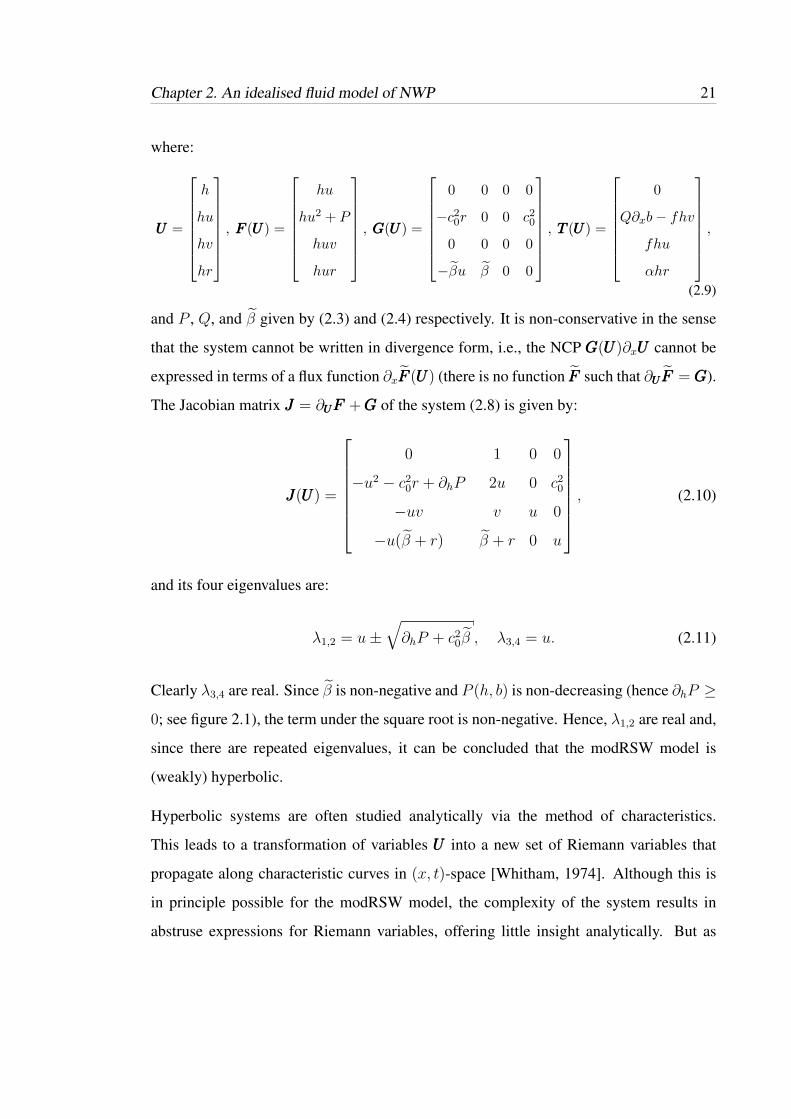
and P , Q, and β given by (2.3) and (2.4) respectively. It is non-conservative in the sense
that the system cannot be written in divergence form, i.e., the NCP GGG(UUU)∂xUUU cannot be
expressed in terms of a flux function ∂xFFF (UUU) (there is no function FFF such that ∂UUUFFF = GGG).
The Jacobian matrix JJJ = ∂UUUFFF +GGG of the system (2.8) is given by:
JJJ(UUU) =
0 1 0 0
−u2 − c20r + ∂hP 2u 0 c20
−uv v u 0
−u(β + r) β + r 0 u
, (2.10)
and its four eigenvalues are:
λ1,2 = u±√∂hP + c20β , λ3,4 = u. (2.11)
Clearly λ3,4 are real. Since β is non-negative and P (h, b) is non-decreasing (hence ∂hP ≥
0; see figure 2.1), the term under the square root is non-negative. Hence, λ1,2 are real and,
since there are repeated eigenvalues, it can be concluded that the modRSW model is
(weakly) hyperbolic.
Hyperbolic systems are often studied analytically via the method of characteristics.
This leads to a transformation of variables UUU into a new set of Riemann variables that
propagate along characteristic curves in (x, t)-space [Whitham, 1974]. Although this is
in principle possible for the modRSW model, the complexity of the system results in
abstruse expressions for Riemann variables, offering little insight analytically. But as

22 Chapter 2. An idealised fluid model of NWP
the prime purpose here is to provide a physically plausibly numerical forecast model for
conducting idealised DA experiments, further Riemann analysis is neglected. However,
one aspect relating to the wave speeds (determined by the eigenvalues) deserves a further
comment. It is well-known that waves travelling through saturated regions of convection
slow down (e.g., Harlim and Majda [2013]). Therefore, simplified models of a moist
atmosphere should reflect this. For example, the SW model of Bouchut et al. [2009] for a
large-scale moist atmosphere has lower wave speeds in ‘moist’ regions compared to dry
regions. For comparison, the eigenvalues of the classical shallow water system (2.1) are:
µ1,2 = u±√p′(h) = u±
√gh , µ3 = u. (2.12)
For the modRSW model (2.2), max|λ1,2| is smaller when Hc < h+ b < Hr, since then
∂hP = 0, and smaller for h + b > Hr when c20β is sufficiently small (specifically, less
than gh), both relative to the standard shallow water case with h + b < Hc. Hence, this
aspect is captured here too.
Non-dimensionalised system
It is useful to work with the non-dimensionalised equations. This acts to simplify
and parametrise the problem, yielding non-dimensional parameters that characterise
the modelled system and embody its dynamics. This is particularly practical for
numerical implementation and comparing quantities that have different physical units.
The dimensionless coordinates and variables are related to their dimensional counterparts
by characteristic scales L0, H0, and V0:
x = L0x, (u, v) = V0(u, v), (h, b,Hc,r) = H0(h, b, Hc,r), r = r. (2.13)

Chapter 2. An idealised fluid model of NWP 23
Then the dimensionless time coordinate and relevant derivatives are:
t = T0t =L0
V0t, ∂x =
1
L0
∂x, ∂t =V0L0
∂t, ∂h =1
H0
∂h. (2.14)
Substituting these into the model equations and defining the non-dimensional effective
pressure p = gH20 p yields the following dimensionless system (with the hats dropped):
∂th+ ∂x(hu) = 0, (2.15a)
∂t(hu) + ∂x(hu2 + P ) +Q∂xb+ hc0
2∂xr −1
Rohv = 0, (2.15b)
∂t(hv) + ∂x(huv) +1
Rohu = 0, (2.15c)
∂t(hr) + ∂x(hur) + hβ∂xu+ αhr = 0, (2.15d)
where:
P (h, b) =1
2Fr2[h2 + ((Hc − b)2 − h2)Θ(h+ b−Hc)
], (2.16)
Q(h, b) =1
Fr2[h+ (Hc − b− h)Θ(h+ b−Hc)] , (2.17)
β = βΘ(h+ b−Hr)Θ(−∂xu), (2.18)
and Θ is the Heaviside function,
Θ(x) =
1, if x > 0;
0, if x ≤ 0.
(2.19)
The following non-dimensional parameters have been introduced:
Fr =V0√gH0
, Ro =V0fL0
, c02 =
c20V 20
, α =L0
V0α. (2.20)

24 Chapter 2. An idealised fluid model of NWP
The Rossby number, Ro, and Froude number, Fr, control the strength of rotation and
stratification respectively compared to the inertial terms uuu · ∇uuu.
2.3 Summary
An idealised fluid model of convective–scale NWP has been outlined, based on the
rotating shallow water equations and extending the model of WC14. The starting point
for the model is the rotating shallow water equations on an f -plane with no variation in
the meridional direction (2.1). In this setting, there are meridional velocity v and Coriolis
rotation effects, while retaining only one spatial dimension.
The mathematical modifications to the parent equations, and the physical arguments
behind the changes, are described in detail in section 2.2. These are strongly motivated
by the model of WC14 (see appendix A) but improve upon it in two ways. First, the
inclusion of v-velocity and rotation means dynamics associated with rotating fluids, such
as geostrophy, are present in the model. Second, and more importantly, the diffusion
terms used to stabilise the model of WC14 have been removed. The dynamics of WC14
are highly sensitive to these terms, specifically the diffusion coefficients Kh, Ku, and
Kr, which are tuned to stabilise the model for a specific set-up and are the dominant
controlling factor of the system’s dynamics. As such, the numerical implementation is
not robust to alterations to, e.g., the bottom topography, the gridsize, and constants α, β,
and γ. Each change requires ad hoc tuning of the diffusion coefficients and integration
time step.
Clearly, it is desirable to simplify this and alleviate the reliance on these arbitrary
coefficients. The hyperbolic character of the model described in this chapter permits
the use of robust numerical techniques developed for hyperbolic systems. The following
chapter makes use of these and derives a novel, stable solver for the idealised fluid model
(2.2).

25
Chapter 3
Numerics
“A day without mistake is a day without mathematics.”1
There exists a powerful class of numerical methods for solving hyperbolic problems,
motivated by the need to capture shock formation in the solutions, a consequence of
nonlinearities in the governing equations. Efficient and accurate finite volume schemes
for systems of conservation laws are very well developed (e.g., LeVeque [2002]; Toro
[2009]). For shallow water models, there are well-balanced schemes that deal accurately
with topography and Coriolis effects, maintaining steady states at rest and non-negative
fluid depth h(x, t) [Audusse et al., 2004; Bouchut, 2007]. However, the nature of the
modRSW model (namely the presence of non-conservative products (NCPs) including
step functions) requires careful treatment beyond the typical methods for conservation
laws. The discontinuous Galerkin finite element method (DGFEM) developed by
Rhebergen et al. [2008] offers a robust method for solving systems of non-conservative
hyperbolic partial differential equations of the form (2.8) but, as will be shown, does not
satisfactorily deal with topography in the SWEs at lowest order. To mitigate this, a novel
scheme is developed here for the modRSW model (2.2) that mixes the NCP theory from
Rhebergen et al. [2008] and the well-balanced scheme of Audusse et al. [2004].1Prof. Jan G. Verwer (1946-2011)

26 Chapter 3. Numerics
The first section introduces the theory of one-dimensional space-DGFEM for hyperbolic
conservation laws. Section 3.2 extends the theory to nonconservative hyperbolic systems,
before the aforementioned issue with topography at lowest order is rigorously investigated
in section 3.3. Finally, the ‘mixed NCP-Audusse’ methodology for the modRSW model
(2.2) is formulated in full. This chapter makes use of two appendices and the reader is
referred to them in the main text when appropriate. The chapter concludes with a concise
summary of the full scheme.
3.1 1D DGFEM for hyperbolic conservation laws
This section addresses the space DGFEM discretisation of nonlinear hyperbolic systems
of conservation laws, i.e., a system of partial differential equations (PDEs) of the form:
∂tUUU + ∂xFFF (UUU) + TTT (UUU) = 0 on Ω = [0, L], (3.1)
where UUU = UUU(x, t) ∈ Rn are the model variables, FFF ∈ Rn is a flux function such
that ∂FFF/∂UUU ∈ Rn×n has real eigenvalues (hence defining the system as, at least
weakly, hyperbolic), and TTT ∈ Rn is linear and contains extraneous forcing terms. The
conservation law (3.1) has initial conditions UUU(x, 0) = UUU0 and specified boundary
conditions:
UUU(0, t) = UUU left, UUU(L, t) = UUU right, (3.2)
typically periodic or inflow/outflow conditions.
3.1.1 Computational mesh
The one-dimensional flow domain Ω = [0, L] is divided into Nel elements Kk =
(xk, xk+1) for k = 1, 2, ..., Nel with Nel + 1 nodes/edges x1, x2, ..., xNel , xNel+1. Element

Chapter 3. Numerics 27
x1 = 0
x2 x3 xNel−1 xNelxNel+1 = L
K0 K1 K2 KNel−1 KNel KNel+1
F1 F2 FNel FNel+1
xk−1 xk xk+1 xk+2
Kk−1 Kk Kk+1
Fk−1 Fk Fk+1 Fk+2
Figure 3.1: The computational mesh Th (3.3) is extended to include a set of ghost elementsK0 and KNel+1 at the boundaries (see section 3.1.4). Central to the DGFEM schemes arethe fluxes numerical F through the nodes, introduced in section 3.1.2.
lengths |Kk| = xk+1 − xk may vary. Formally, one can define a tessellation Th of the Nel
elements Kk:
Th = Kk :
Nel⋃k=1
Kk = Ω, Kk ∩Kk′ = ∅ if k 6= k′, 1 ≤ k, k′ ≤ Nel, (3.3)
where overbar denotes closure Ω = Ω ∪ ∂Ω. This simply means that the elements Kk
cover the whole domain and do not overlap. A schematic of the mesh is shown in figure
3.1; the concept of flux functions and ghost elements is introduced in sections 3.1.2 and
3.1.4 respectively.
3.1.2 Weak formulation
The first step of any finite element method is to convert the PDE of interest into its
equivalent weak formulation using the standard test function and integration approach
(e.g., Zienkiewicz et al. [2014]):
(i) multiply the system (3.1) by an arbitrary test function w ∈ C1(Kk), generally

28 Chapter 3. Numerics
continuous on each element but discontinuous across an element boundary;
(ii) integrate by parts over each element Kk and sum over all elements;
(iii) replace the exact model states UUU and test functions w by approximations UUUh, wh,
and, where appropriate, the flux function FFF by a numerical flux F .
Steps (i) and (ii)
Proceeding thus with the multiplication and integration:
0 =
Nel∑k=1
∫Kk
[w∂tUUU + w∂xFFF (UUU) + wTTT (UUU)] dx
=
Nel∑k=1
∫Kk
[w∂tUUU + ∂x(wFFF (UUU))−FFF (UUU)∂xw + wTTT (UUU)] dx
=
Nel∑k=1
∫Kk
[w∂tUUU −FFF (UUU)∂xw + wTTT (UUU)] dx+[w(x−k+1)FFF (x−k+1)− w(x+k )FFF (x+k )
] (3.4)
where w(x−k+1) = limx↑xk+1w(x), w(x+k ) = limx↓xk w(x), and FFF (x±k ) is to be read as
FFF (UUU(x±k , t)). Reworking the summation of the fluxes over elements, terms evaluated at
the interior (k = 2, ..., Nel) and exterior (k = 1, Nel + 1) nodes are isolated:
Nel∑k=1
[w(x−k+1)FFF (x−k+1)− w(x+k )FFF (x+k )
]= w(x−Nel+1)FFF (x−Nel+1)− w(x+1 )FFF (x+1 )
+
Nel∑k=2
[w(x−k )FFF (x−k )− w(x+k )FFF (x+k )
]︸ ︷︷ ︸=:wLFFFL−wRFFFR
, (3.5)
with superscript L,R denoting evaluation left or right of node xk. The average of a
quantity is denoted by · = 12((·)L + (·)R) and the difference by J·K = (·)L − (·)R.

Chapter 3. Numerics 29
Then the flux at the interior nodes can be written:
wLFFFL − wRFFFR = JwK(γ1FFFL + γ2FFFR) + JFFF K(γ1wR + γ2w
L)
= JwK(γ1FFFL + γ2FFFR), (3.6)
with γ1 + γ2 = 1 and after imposing flux conservation at a node, i.e., continuity of FFF :
JFFF K = 0. Then the weak formulation (3.4) reads:
0 =
Nel∑k=1
∫Kk
[w∂tUUU −FFF (UUU)∂xw + wTTT (UUU)] dx
+[w(x−Nel+1)FFF (x−Nel+1)− w(x+1 )FFF (x+1 )
]+
Nel∑k=2
JwK(γ1FFFL + γ2FFFR). (3.7)
Step (iii)
Since continuity of FFF has been enforced above, it suggests that the fluxes FFFL and FFFR
through each node should be replaced by the same numerical flux F that depends on
variable values to the left and right of that node:
Fk = FFF (UUU(x−k ),UUU(x+k )). (3.8)
It follows that (γ1FFFL + γ2FFF
R) = F and, after replacing the model states UUU and test
functions w by approximations UUUh, wh in (3.7), the discretised weak form reads:
0 =
Nel∑k=1
∫Kk
[wh∂tUUUh −FFF (UUUh)∂xwh + whTTT (UUUh)] dx
+ wh(x−Nel+1)FFF (UUUh(x
−Nel+1),UUU right)− wh(x+1 )FFF (UUU left,UUUh(x
+1 ))
+
Nel∑k=2
(wh(x
−k )− wh(x+k )
)FFF (UUUh(x
−k ),UUUh(x
+k )), (3.9)
30 Chapter 3. Numerics
where the values UUUh(x−1 ) = UUU left and UUUh(x
+Nel+1) = UUU right are chosen to enforce the
boundary conditions (3.2). The approximations UUUh and wh are defined by expansions
in terms of polynomial basis functions of degree dp, with dp determining the order of the
scheme. Typical choices for the numerical flux are the Lax-Friedrichs flux or approximate
Riemann solvers such as the HLL or HLLC flux (see, e.g., Toro [2009]).
3.1.3 Space-DG0 discretisation
This thesis is concerned with the lowest order scheme dp = 0; the reasons behind this are
explained in section 3.4. The zero-order expansion (so-called DG0) yields a piecewise
constant approximation in each element:
UUUh(x, t) = Uk(t) =1
|Kk|
∫Kk
UUU(x, t)dx. (3.10)
Inserting this in (3.9) and, since the test functionwh is arbitrary, settingwh = 1 alternately
in each element, the DG0-discretisation for each element reads:
0 =dUk
dt+Fk+1 −Fk|Kk|
+ TTT (Uk), (3.11)
where Fk = FFF (U−k , U+k ) is the numerical flux to be defined, and typically U−k = Uk−1,
U+k = Uk since the values are constant in an element. This is equivalent to a ‘Finite
Volume’ (FV) Godunov scheme in one dimension (e.g., LeVeque [2002]).
3.1.4 Boundary conditions and ghost elements
It is apparent from sections 3.1.2 and 3.1.3 that computing the fluxes and updating each
elementKk requires information from neighbouring elementsKk−1 andKk+1, known as a
‘three-point stencil’ since the update algorithm spans three elements. For k = 2, ..., Nel−

Chapter 3. Numerics 31
1, this is provided by updates in time of the computational values (3.10). However, in the
first and last elements of the mesh, K1 and KNel , the required neighbouring information
is not present and the physical boundary conditions (3.2) must be used in updating these
elements. Typically, this is achieved by extending the computational mesh with so-called
‘ghost’ elements (see figure 3.1 and, e.g., LeVeque [2002], chapter 7). The ghost elements
K0, KNel+1 are used to update the fluxes F1, FNel+1 at x1 = 0, xNel+1 = L, respectively.
Values in these elements are set at the beginning of each time-step in a way that takes
into consideration the boundary conditions, and the updating algorithm is then exactly the
same in every element. Two common types of boundary condition, and the two used in
this thesis, are ‘periodic’ and ‘outflow’.
Periodic boundaries
Periodic boundary conditions have the form UUU(0, t) = UUU(L, t). To implement this
condition numerically, values to the left of node x1 in ghost element K0 should be the
same as those to the left of node xNel+1 in KNel , and values to the right of node xNel+1
in KNel+1 should be the same as those to the right of node x1 in K1. This is achieved by
setting
U−1 = U−Nel+1, U+Nel+1 = U+
1 , (3.12)
at the start of each time-step. For the standard DG0 scheme (3.11), this impliesU0 = UNel
and UNel+1 = U1. It follows that F1 = FNel+1 and periodicity is ensured.
Outflow boundaries
Outflow boundary conditions mean that the fluid is allowed to leave the flow domain in
a physically-consistent manner, essentially setting the domain to be infinitely large. In
this case, the required information is typically extrapolated from the interior solution.
Care needs to be taken when implementing outflow conditions to ensure that the specified

32 Chapter 3. Numerics
boundary information does not contaminate the interior solution. Outgoing waves should
propagate out of the domain without generating spurious reflections from the artificial
boundary [LeVeque, 2002]. The simplest, yet extremely powerful and effective, approach
uses a zero-order extrapolation [LeVeque, 2002], meaning extrapolation by a constant
function, and sets
U−1 = U+1 , U+
Nel+1 = U−Nel+1, (3.13)
at the start of each time-step. For the standard DG0 scheme (3.11), this implies U0 = U1
and UNel+1 = UNel .
3.2 1D DGFEM for non-conservative hyperbolic PDEs
In this section, following the DGFEM weak formulation for conservation laws, a method
is derived for solving nonlinear hyperbolic systems of PDEs in non-conservative form:
∂tUUU + ∂xFFF (UUU) +GGG(UUU)∂xUUU + TTT (UUU) = 0, (3.14)
where UUU ∈ Rn are the model variables, FFF ∈ Rn is a flux function,GGG ∈ Rn×n is the NCP
matrix, and TTT ∈ Rn is linear and contains extraneous forcing terms. Since the system is
hyperbolic, ∂FFF/∂UUU +GGG ∈ Rn×n has real eigenvalues. It is non-conservative in the sense
that GGG(UUU)∂xUUU cannot be expressed in terms of a flux function ∂xFFF (UUU), i.e., there is no
function FFF such that ∂UUUFFF = GGG. Alternatively, the system (2.8) can be written:
∂tUUU +DDD(UUU)∂xUUU + TTT (UUU) = 0, (3.15)
whereDDD = ∂FFF/∂UUU +GGG ∈ Rn×n.
The DGFEM theory for non-conservative hyperbolic PDEs in multi-dimensions has been
developed by Rhebergen et al. (2008). Crucial to the weak formulation derived for

Chapter 3. Numerics 33
equations of the form (3.14) is the work of Dal Maso, LeFloch, and Murat (DLM;
Dal Maso et al. [1995]). This so-called DLM theory is used to overcome the absence
of a weak solution due to the non-conservative productsGGG(UUU)∂xUUU .
3.2.1 DLM theory
Le Floch [1989] illustrates the DLM theory using the following example. Consider a
single non-conservative product (NCP) g(u)∂xu where g : Rn → Rn is a smooth function
but u : [a, b]→ Rn may admit discontinuities. E.g.:
u(x) = uL + Θ(x− xd)(uR − uL) (3.16)
where uL,R ∈ Rn are constant vectors, xd ∈ [a, b], and Θ : R → R is the Heaviside
function (Θ(x) = 1 if x > 0; and 0 if x ≤ 0). For any smooth function g : Rn → Rn, the
NCP g(u)∂xu with (3.16) is not defined at x = xd since |∂xu| → ∞ here. To overcome
this, a smooth regularisation uε of the discontinuous u is introduced:
g(u)du
dx≡ lim
ε→0g(uε)
duε
dx. (3.17)
Such a regularisation of u enables the NCP to be defined as a bounded measure and gives
sense to a weak formulation of the PDEs. The limit in (3.17) depends on the choice of
uε. To define the regularisation, introduce a Lipschitz continuous path φ : [0, 1] → Rn
satisfying φ(0) = uL and φ(1) = uR and connecting uL to uR in Rn. The following
regularisation arises, defined for ε > 0:
uε(x) =
uL, if x ∈ [a, xd − ε];
φ(x−xd+ε2ε
), if x ∈ [xd − ε, xd + ε];
uR, if x ∈ [xd − ε, b].
(3.18)

34 Chapter 3. Numerics
Using this, Le Floch [1989] states that:
limε→0
g(uε)duε
dx= Cδxd , with C =
∫ 1
0
g(φ(τ))∂φ
∂τ(τ)dτ, (3.19)
where δxd is the Dirac measure at xd. The regularisation in the limit ε→ 0 clearly depends
on the path φ, except when g is in fact conservative, i.e., ∃q : Rn → R with g = ∂xq. If
this is the case then C = q(φ(1))− q(φ(0)) = q(uR)− q(uL).
It is this formulation, namely that of the NCP as a bounded measure, that enables
the weak formulation to be derived for equations of the form (3.14). In DGFEM, the
computational states are generally continuous on each element but discontinuous across
an element boundary. It is in this context that the framework afforded by the DLM theory
(and culminating in (3.19)) appears naturally in the weak formulation and subsequent
discretisation, cf. (3.21) and (3.22) in section 3.2.2. A full derivation, including the
key theorems employed from the DLM theory, is given by Rhebergen et al. [2008]. A
summary is given in the next section.
3.2.2 Weak formulation
The space DGFEM weak formulation for the system (3.14) with linear source terms SSS is
given by equation (A.11) in Rhebergen et al. [2008] and below here. In the following,
repeated indices are used for the summation convention with i, j = 1, ..., 4 denoting
components of vectors. In one space dimension and considering cell Kk only, the weak
form reads:
0 =
∫Kk
[w∂tUi − Fi∂xw + wGij∂xUj + wTi] dx
+[w(x−k+1)P
pi (x−k+1, x
+k+1)− w(x+k )Pmi (x−k , x
+k )], (3.20)

Chapter 3. Numerics 35
where Pp and Pm are given by:
Pp = PNC +1
2
∫ 1
0
Gij(φφφ)∂φj∂τ
dτ, (3.21a)
Pm = PNC − 1
2
∫ 1
0
Gij(φφφ)∂φj∂τ
dτ, (3.21b)
and the NCP flux is:
PNCi (UUUL,UUUR) =
FLi − 1
2
∫ 1
0Gij(φφφ)
∂φj∂τ
dτ, if SL > 0;
FHLLi − 1
2SL+SR
SR−SL∫ 1
0Gij(φφφ)
∂φj∂τ
dτ, if SL < 0 < SR;
FRi + 1
2
∫ 1
0Gij(φφφ)
∂φj∂τ
dτ, if SR < 0;
(3.22)
Here, FHLLi is the standard HLL numerical flux [Harten et al., 1983]:
FHLLi =
FLi S
R − FRi S
L + SLSR(URi − UL
i )
SR − SL, (3.23)
Gij is the ij-th element of the matrix GGG, and SL,R are the fastest left- and right-moving
signal velocities in the solution of the Riemann problem, determined by the eigenvalues
of the Jacobian ∂FFF/∂UUU +GGG of the system.
3.2.3 Space-DG0 discretisation
Using piecewise constant basis functions, we take U ≈ Uh = Uk(t) and, since the test
function w ≈ wh is arbitrary, wh = 1 alternately in each element. The semi-discrete
space-DGFEM scheme for element Kk reads:
0 = |Kk|dUk
dt+ Pp(U−k+1, U
+k+1)− P
m(U−k , U+k ) + |Kk|T k, (3.24)
where U−k+1 = Uk, U+k+1 = Uk+1, U−k = Uk−1, U+
k = Uk, and T k = TTT (Uk). This is
equivalent to a ‘Finite Volume’ (FV) Godunov scheme in one dimension.

36 Chapter 3. Numerics
3.3 SWEs: issues with well-balancedness at DG0
In principle, the topography b in the idealised fluid model (2.2) can be treated as a model
variable (b = b(x, t) with ∂tb = 0) such that the topographic source term Q∂xb in
(2.9) is then treated as an NCP. However, hitherto less well-known issues with ‘well-
balancedness’ for DG0 discretisations with varying topography mean this approach is
unsatisfactory. A numerical scheme is well-balanced if trivial steady states (e.g., rest
flow) are satisfied, i.e., rest flow remains at rest in the numerical solution. These issues
are addressed in this section. To do so, it is sufficient to consider the non-rotating shallow
water system with non-zero bottom topography:
∂th+ ∂x(hu) = 0, (3.25a)
∂t(hu) + ∂x
(hu2 +
1
2gh2)
= −gh∂xb, (3.25b)
∂tb = 0, (3.25c)
which can be expressed in non-conservative form (3.14) with:
UUU =
h
hu
b
, FFF (UUU) =
hu
hu2 + 12gh2
0
, GGG(UUU) =
0 0 0
0 0 gh
0 0 0
. (3.26)
The eigenvalues of the Jacobian ∂FFF/∂UUU +GGG are λ± = u±√gh and λ0 = 0, which give
the following numerical speeds:
SL = min(uL −
√ghL , uR −
√ghR
), (3.27a)
SR = max(uL +
√ghL , uR +
√ghR
). (3.27b)
Chapter 3. Numerics 37
For i = 1, 3, there are no NCPs in the equations so contributions to the integrals in
(3.21) and (3.22) are zero. For i = 2 and employing a linear path φφφ(τ ;UUUL,UUUR) =
UUUL + τ(UUUR −UUUL):
∫ 1
0
G2j(φφφ)∂φj∂τ
dτ =
∫ 1
0
g(hL + τ(hR − hL))(bR − bL)dτ
= g(bR − bL)
∫ 1
0
(hL + τ(hR − hL))dτ
= g(bR − bL)
[hLτ +
1
2τ 2(hr − hL)
]10
= g(bR − bL)1
2(hL + hR)
= −gJbKh, (3.28)
recalling that · = 12((·)L + (·)R) and J·K = (·)L − (·)R. It is shown analytically here
that when taking a linear path and piecewise constant DG0 approximation for the model
states and test functions, the resulting scheme is not well-balanced. Flow at rest requires
that the free surface height remains constant bL + hL = bR + hR with uL = uR = 0.
Under these conditions, SL < 0 < SR always and so the NCP flux (3.22) is:
PNCi = FHLLi − 1
2
SL + SR
SR − SLV NCi (3.29)
where V NCi is given by (3.28) for i = 2 and zero for i = 1, 3. Since F1 = hu = 0 for rest
flow and F3 = 0, the fluxes for the h- and b-equations are:
PNC1 =SLSR(hR − hL)
SR − SL, PNC3 =
SLSR(bR − bL)
SR − SL, (3.30)
and by (3.21) we have that Pp1 = Pm1 = PNC1 and Pp3 = Pm3 = PNC3 . For the hu-
equation, we note that U2 = hu = 0, F2 = 12gh2 and V NC
2 = 12g((hL)2 − (hR)2) for rest

38 Chapter 3. Numerics
flow and so the flux is:
PNC2 =1
SR − SL[SRFL
2 − SLFR2 −
1
2(SL + SR)V NC
2
]=
1
SR − SL[1
2SRg(hL)2 − 1
2SLg(hR)2 − 1
4(SL + SR)g((hL)2 − (hR)2)
]=
1
4g
1
SR − SL[SR(hL)2 − SL(hR)2 − SL(hL)2 + SR(hR)2)
]=
1
4g
1
SR − SL[(SR − SL)((hL)2 + (hR)2)
]=
1
4g((hL)2 + (hR)2), (3.31)
=⇒ Pp2 = PNC2 +1
2V NC2
=1
4g((hL)2 + (hR)2) +
1
4g((hL)2 − (hR)2)
=1
2g(hL)2, (3.32)
=⇒ Pm2 = PNC2 − 1
2V NC2
=1
4g((hL)2 + (hR)2)− 1
4g((hL)2 − (hR)2)
=1
2g(hR)2. (3.33)
To summarise:
Pp =
SLSR(hR−hL)
SR−SL
12g(hL)2
SLSR(bR−bL)SR−SL
, Pm =
SLSR(hR−hL)
SR−SL
12g(hR)2
SLSR(bR−bL)SR−SL
, (3.34)
Using piecewise constant basis functions w ≈ wh = 1 alternately in each element and
U ≈ Uh = Uk(t), the space-DG0 scheme for element Kk reads:
0 = |Kk|dUk
dt+ Pp(U−k+1, U
+k+1)− P
m(U−k , U+k ), (3.35)

Chapter 3. Numerics 39
where U−k+1 = Uk, U+k+1 = Uk+1, U−k = Uk−1, U+
k = Uk and so:
Pp =
SLk+1S
Rk+1(hk+1−hk)
SRk+1−SLk+1
12gh2k
SLk+1SRk+1(bk+1−bk)
SRk+1−SLk+1
, Pm =
SLk S
Rk (hk−hk−1)
SRk −SLk
12gh2k
SLk SRk (bk−bk−1)
SRk −SLk
, (3.36)
We prove rest flow remains at rest by considering the evolution of hu and h + b as
determined by the DG0 discretisation (3.24):
hu : 0 = |Kk|d
dt(huk) +
1
2gh2k −
1
2gh2k =⇒ d
dt(huk) = 0, (3.37)
h+ b : 0 = |Kk|d
dt(hk + bk) +
SLk+1SRk+1(hk+1 − hk + bk+1 − bk)
SRk+1 − SLk+1
− SLk SRk (hk − hk−1 + bk − bk−1)
SRk − SLk=⇒ d
dt(hk + bk) = 0, (3.38)
since hL + bL = hR + bR. Thus, the free surface height h + b remains constant for rest
flow. However, consider the evolution of b only:
0 = |Kk|d
dt(bk) +
SLk+1SRk+1(bk+1 − bk)
SRk+1 − SLk+1
− SLk SRk (bk − bk−1)SRk − SLk
, (3.39)
and note that the evolution equation for h is the same as this after replacing b with h
everywhere. Since b ≈ bh is discontinuous at the nodes for non-constant b, the sum of
the flux terms is non-zero, leading to evolving topography. The same is true for h. Thus,
although flow remains at rest in the sense that h + b = 0, the DG0 scheme is not well-
balanced since d(bk)/dt 6= 0 and d(hk)/dt 6= 0. For DG1 expansions (and higher), we
can project the DG expansion coefficients of b such that bh remains continuous across
elements, then bR = bL and d(bk)/dt = 0. Then all aspects of rest flow are satisfied
numerically and the scheme is truly well-balanced. A proof is given in appendix C.

40 Chapter 3. Numerics
3.4 Numerical formulation: modRSW
3.4.1 Approach: a mixed NCP-Audusse scheme
Since the goal here is a toy model for DA research, it is preferable to keep the scheme
as computationally efficient as possible and acknowledge higher-order accuracy as of
secondary importance. However, as was shown in section 3.3, there are issues with well-
balancedness for DG0 discretisations with varying topography. In order to remain at
DG0, the topographic source term is discretised directly using the established method of
Audusse et al. [2004], resulting in a well-balanced scheme at lowest order that efficiently
preserves non-negativity of fluid depth h. It is first necessary to isolate the topographic
source term in (2.9) from the other terms pertaining to rotation and removal of rain:
TTT (UUU) = TTTO(UUU) + TTTB(UUU) = [0,−fhv, fhu, αhr]T + [0, Q∂xb, 0, 0]T . Then TTTO is
discretised as a standard linear extraneous forcing term andTTTB via the method of Audusse
et al. [2004].
Using piecewise constant basis functions UUU ≈ UUUh = Uk(t) and wh = 1 alternately in
each element (since the test function w ≈ wh is arbitrary), the semi-discrete space-DG0
scheme (3.24) for element Kk ∈ Th reads:
0 = |Kk|dUk
dt+ Pp(U−k+1, U
+k+1)− P
m(U−k , U+k ) + |Kk|TOk + TBk , (3.40)
whereU±k are reconstructed states to the left and right of node xk, and TBk is the discretised
topographic source term. The flux terms Pp and Pm are given by (3.21) and the NCP flux
PNC (3.22) needs deriving for the modRSW system (2.8, 2.9). Before deriving the fluxes,
the scheme of Audusse et al. [2004] to discretise TBk and define the reconstructed states
U±k is outlined.

Chapter 3. Numerics 41
3.4.2 Discretising the topographic source term
In Audusse et al. [2004], a well-balanced scheme is derived for solving the shallow water
equations with non-flat topography. The two main developments to achieve this are: (i)
using reconstructed computational states U−k and U+k to the left and right of an element
edge in the numerical flux instead of cell-centred values Uk−1 and Uk; and (ii) discretising
the topographic source term by considering the leading order balancing requirement for
nearly hydrostatic flows. A summary is given here; for full details the reader is referred
to section 2 of Audusse et al. [2004].
In the asymptotic limit for nearly hydrostatic flows the leading order fluid depth h adjusts
so as to satisfy the balance of momentum flux and momentum source terms:
∂x (p(h)) = ∂x
(1
2gh2)
= −gh∂xb. (3.41)
This also ensures that the ‘lake at rest’ property (i.e., the trivial steady state solution u = 0
and h + b = constant) is satisfied. Integrating over element Kk yields an approximation
to the topographic source term in the form of a flux:
−∫Kk
gh∂xbdx =1
2g(h−k+1)
2 − 1
2g(h+k )2 = p(h−k+1)− p(h
+k ). (3.42)
The reconstructions for the leading order fluid depth:
h−k = hk−1 + bk−1 −max(bk−1, bk), (3.43a)
h+k = hk + bk −max(bk−1, bk), (3.43b)
and are truncated to ensure non-negativity of the depth: h±k = max(0, h±k ). Note that a
modified CFL condition imposes an elemental time-step restriction also required to ensure
both stability and non-negativity. This is shown in appendix B; the time-step is given by
(B.21–B.22). The reconstructed computational states U±k to the left and right of node xk
42 Chapter 3. Numerics
are:
U−k =
h−k
h−k uk−1
h−k vk−1
h−k rk−1
, U+k =
h+k
h+k uk
h+k vk
h+k rk
. (3.44)
The fluxes in (3.21) and (3.22) are evaluated using these reconstructions and the
discretised topographic source term TBk in (3.40) is:
TBk =
0
P (h−k+1, b−k+1)− P (h+k , b
+k )
0
0
, (3.45)
for P defined in (2.3). The resulting scheme satisfies ’flow at rest’ for h + b < Hc,
Hc < h+ b < Hr, and h+ b > Hr.
3.4.3 NCP flux: derivation
The NCP flux PNCi (3.22) is derived for i = 1, ..., 4 in this section for a linear path
φφφ(τ ;UUUL,UUUR) = UUUL + τ(UUUR − UUUL). The integrands involve calculations from the rows
of the ‘non-conservative’ GGG matrix in equation (2.9). It is clear from (3.22) that in the
absence of non-conservative products (Gij = 0 for all i, j) the numerical flux reduces
exactly to the standard HLL flux (3.23). However, for Gij 6= 0, the NCP contributions of
the form in (3.17) must be calculated. The fastest left- and right-moving signal velocities
SL,R are determined by the eigenvalues (2.11) of the Jacobian of the system:
SL = min
(uL −
√(∂hP )|L + c20β|L , uR −
√(∂hP )|R + c20β|R
), (3.46a)
SR = max
(uL +
√(∂hP )|L + c20β|L , uR +
√(∂hP )|R + c20β|R
). (3.46b)

Chapter 3. Numerics 43
It helps to define P = P (h, b) and Q = Q(h, b) in terms of the Heaviside function Θ
(2.19):
P (h, b) =1
2g[h2 + ((Hc − b)2 − h2)Θ(h+ b−Hc)
](3.47a)
Q(h, b) = g [h+ (Hc − b− h)Θ(h+ b−Hc)] (3.47b)
and note the following properties of Θ:
d
dτ[τΘ(τ)] = Θ(τ),
d
dτ
[1
2τ 2Θ(τ)
]= τΘ(τ). (3.48)
For i = 1, 3, the non-conservative products are zero since the first and third rows of the
matrix GGG have zero entries only. Thus, the integrals in the flux (3.22) are zero and PNC
reduces to the HLL flux (3.23).
For i = 2, the integrand to be calculated is:
G2j(φφφ)∂φj∂τ
= G21(φφφ)∂φ1
∂τ+G24(φφφ)
∂φ4
∂τ
= −c20(rL + τ(rR − rL))(hR − hL) + c20(hRrR − hLrL)
= c20(JhK(rL − τJrK)− JhrK
), (3.49)
recalling that J·K denotes the jump of a quantity across a node, J·K = (·)L − (·)R.
Integrating over τ ∈ [0, 1] yields:
∫ 1
0
(c20JhK(r
L − τJrK)− c20JhrK)
dτ = c20JhK∫ 1
0
(rL − τJrK)dτ − c20JhrK∫ 1
0
dτ
= c20
(JhK(rL +
1
2(rR − rL))− JhrK
)= −c20JrKh. (3.50)

44 Chapter 3. Numerics
Thus, the expression to be inserted in the flux function (3.22) then becomes:
∫ 1
0
G2j(φφφ)∂φj∂τ
dτ = −c20JrKh (3.51)
Thus, for SL > 0, the numerical flux is:
PNC2 = FL2 −
1
2
(−c20JrKh
), (3.52)
while for SR < 0:
PNC2 = FR2 +
1
2
(−c20JrKh
), (3.53)
and for SL < 0 < SR:
PNC2 = FHLL2 − 1
2
SL + SR
SR − SL
∫ 1
0
G2j(φφφ)∂φj∂τ
dτ
= FHLL2 − 1
2
SL + SR
SR − SL
(− c20JrKh
). (3.54)
For i = 4, the integrand includes the β term, the switch dependent on model variables
h, u and topography b. We have that:
G4j(φφφ)∂φj∂τ
= G41(φφφ)∂φ1
∂τ+G42(φφφ)
∂φ2
∂τ
= −β(uL + τ(uR − uL))(hR − hL)
)+ β(hRuR − hLuL)
= β(JhK(uL + τ(uR − uL))− JhuK
), (3.55)

Chapter 3. Numerics 45
and so the integral to be computed in the flux is:
∫ 1
0
G4j(φφφ)∂φj∂τ
dτ =
∫ 1
0
β(JhK(uL + τ(uR − uL))− JhuK
)dτ
= JhK∫ 1
0
β(uL + τ(uR − uL))dτ − JhuK∫ 1
0
βdτ
=(JhKuL − JhuK
)∫ 1
0
βdτ − JhKJuK∫ 1
0
τ βdτ. (3.56)
To proceed, we set z = h + b and consider β defined by equation (2.4) but with z =
zL + τ(zR − zL) and u = uL + τ(uR − uL), so that β is a function of τ :
β = βΘ(zL + τ(zR − zL)−Hr)Θ(−∂xu). (3.57)
It is apparent that Θ(−∂xu) depends on the end points of φ only, and is therefore
independent of τ . If uL < uR then ∂xu > 0, and if uL > uR then ∂xu < 0. Thus
Θ(−∂xu) is equivalent to Θ(uL − uR) = Θ(JuK). It should be noted that this argument
is valid for piecewise constant numerical profiles only, i.e., cell averages. A scheme
that approximates continuous profiles using means and slopes would require greater
consideration.
First, we compute the integral of β over [0, 1]:
∫ 1
0
βdτ =
∫ 1
0
βΘ(zL + τ(zR − zL)−Hr)Θ(−∂xu)dτ
= βΘ(JuK)∫ 1
0
Θ(zL + τ(zR − zL)−Hr)dτ
= βΘ(JuK)∫ 1
0
Θ(Xτ + Y )dτ︸ ︷︷ ︸Iβ
, (3.58)

46 Chapter 3. Numerics
where X = zR − zL = −JzK and Y = zL −Hr. When X = 0, this integral is trivial:
∫ 1
0
βdτ = βΘ(JuK)∫ 1
0
Θ(Y )dτ = βΘ(JuK)Θ(Y ). (3.59)
For X 6= 0, a change of variable ξ = Xτ + Y and integration yields:
∫ 1
0
βdτ =β
XΘ(JuK)
∫ X+Y
Y
Θ(ξ)dξ =β
XΘ(JuK) [ξΘ(ξ)]X+Y
Y
=β
XΘ(JuK) [(X + Y )Θ(X + Y )− YΘ(Y )] .
(3.60)
Hence,
∫ 1
0
βdτ = βΘ(JuK)Iβ,
where: Iβ =
Θ(Y ), if X = 0;
(X+Y )X
Θ(X + Y )− YX
Θ(Y ) if X 6= 0.
(3.61)
Intuitively, this makes sense: when X + Y < 0 and Y < 0 (i.e., zR < Hr and zL < Hr),
the rain threshold has not been exceeded, meaning no rain is produced, and the above
integral is zero.
Proceeding in the same manner, we compute the integral of the product τ β over [0, 1]:
∫ 1
0
τ βdτ = βΘ(JuK)∫ 1
0
τΘ(Xτ + Y )dτ︸ ︷︷ ︸Iτβ
. (3.62)
Again, when X = 0, this integral is trivial:
Iτβ =
∫ 1
0
τΘ(Y )dτ =1
2Θ(Y ). (3.63)

Chapter 3. Numerics 47
For X 6= 0, a change of variable ξ = Xτ + Y and integration yields:
Iτβ =1
X2
∫ X+Y
Y
(ξ − Y )Θ(ξ)dξ =1
X2
[1
2ξ2Θ(ξ)− Y ξΘ(ξ)
]X+Y
Y
, using (3.48)
=1
2X−2
[(X2 − Y 2
)Θ(X + Y ) + Y 2Θ(Y )
].
(3.64)
Hence,
∫ 1
0
τ βdτ = βΘ(JuK)Iτβ,
where: Iτβ =1
2
Θ(Y ), if X = 0;
X−2[(X2 − Y 2)Θ(X + Y ) + Y 2Θ(Y )], if X 6= 0.
(3.65)
Equation (3.56) now reads:
∫ 1
0
G4j(φφφ)∂φj∂τ
dτ =(JhKuL − JhuK
)∫ 1
0
βdτ − JhKJuK∫ 1
0
τ βdτ
= βΘ(JuK)(
(JhKuL − JhuK)Iβ − JhKJuKIτβ)
= −βJuKΘ(JuK)(hRIβ + JhKIτβ
). (3.66)
Thus, for SL > 0, the numerical flux is:
PNC4 = FL4 +
1
2βJuKΘ(JuK)
(hRIβ + JhKIτβ
), (3.67)
while for SR < 0:
PNC4 = FR4 −
1
2βJuKΘ(JuK)
(hRIβ + JhKIτβ
), (3.68)

48 Chapter 3. Numerics
and finally for SL < 0 < SR:
PNC4 = FHLL4 +
1
2
SL + SR
SR − SLβJuKΘ(JuK)
(hRIβ + JhKIτβ
). (3.69)
This completes the calculations; the NCP flux in vector form is summarised as follows:
PNC(UL, UR) =
FFFL − 1
2VVV NC , if SL > 0;
FFFHLL − 12SL+SR
SR−SLVVVNC , if SL < 0 < SR;
FFFR + 12VVV NC , if SR < 0;
(3.70)
where FFFHLL is the HLL numerical flux:
FFFHLL =FFFLSR −FFFRSL + SLSR(UR − UL)
SR − SL, (3.71)
and VVV NC arises due to the non-conservative products:
VVV NC =
0
−c20JrKh
0
−βJuKΘ(JuK)(hRIβ + JhKIτβ
)
. (3.72)
where Iβ and Iτβ are given by (3.61) and (3.65), respectively.

Chapter 3. Numerics 49
3.4.4 Outline: mixed NCP-Audusse scheme
The final part of this section provides a concise summary of the full mixed NCP-Audusse
scheme. The semi-discrete DG0 scheme reads:
0 = |Kk|dUk
dt+ |Kk|TOk + TBk + Pp(U−k+1, U
+k+1)− P
m(U−k , U+k ), (3.73)
where:
• Uk = [hk, huk, hvk, hrk]T and U±k are the reconstructed states (3.44);
• TOk = TTTO(Uk) where TTTO = [0,−fhv, fhu, αhr]T and TBk is the discretised
topographic source term (3.45);
• the flux terms Pp,m are given by (3.21) and the NCP flux PNC has been derived in
section 3.4.3, culminating in equations (3.70–3.72);
• the expressions containing Heaviside functions associated with the thresholds Hc
and Hr in the fluxes are Iβ (3.61) and Iτβ (3.65).
Non-negativity is ensured using the time step (B.21–B.22) derived in appendix B for the
time discretisation.

50 Chapter 3. Numerics

51
Chapter 4
Dynamics
“... moist convection is many things...”1
A recurring theme throughout Stevens [2005] review of atmospheric moist convection is
the sheer complexities and intricacies of the subject. Manifest as clouds, it comprises a
variety of regimes spanning a vast range of spatial and temporal scales, with diverse and
nonlinear physical processes in each regime; hence, he concludes, it is many things. The
most powerful state-of-the-art numerical models of the atmosphere struggle with their
treatment of moist convection, and so an idealised model of convection and precipitation
is naturally limited in what it can expect to capture. However, as described in chapter
2, one can seek to represent some of the fundamental processes and aspects of moist
convection in a relatively simple modelling environment. In this chapter, the dynamics
of the idealised fluid model (2.2) are investigated numerically using the methodology
described in chapter 3.
1 Stevens [2005]

52 Chapter 4. Dynamics
4.1 Numerical experiments
This section presents the results of experiments that have been chosen specifically to
highlight the dynamics of the modified rotating shallow water model (2.2) compared to
those of the classical model (2.1). The experiments are based on: (i) a Rossby adjustment
scenario, and (ii) non-rotating flow over topography, both of which have a rich history in
shallow water theory including known exact steady state solutions. To illustrate the effect
that exceeding the threshold heights Hc < Hr has on the dynamics, a hierarchy of model
‘cases’ is employed:
• Case I: h + b < Hc always (effectively setting Hc, Hr → ∞). The model (2.2)
reduces to standard (rotating) SWEs (2.1) if hr = 0 initially.
• Case II: h + b < Hr always, but may exceed Hc. This is considered a ‘stepping
stone’ to the full model to isolate the effect of the first threshold exceedance. Thus,
givenHc exceedance and the consequent modification to the gradient of the pressure
(2.3a), we expect the fluid to be forced upwards (a ‘convective updraft’).
• Case III: h + b may exceed both Hc, Hr (and ∂xu < 0). This is the full model
with convection and rain processes to be used for idealised convective-scale DA
research.
For the modRSW model to have credibility as a shallow water-type model, it is crucial
that it reproduces, in case I, known results of the standard shallow water equations.
The existence of exact steady state solutions thus provides a benchmark to test this and
the solutions can be used as reference states to compare the subsequent modifications
introduced by cases II and III. The non-dimensionalised equations (section 2.2) are
implemented on a domain of unit length using the mixed NCP-Audusse numerical scheme
summarised in section 3.4.4 and the forward Euler time discretisation. All simulations in

Chapter 4. Dynamics 53
0
0.25
0.5
0.75
1
0.2
0.4
0.6
0.8
1
0
1
2
3
4
xt
h(x
,t)
0
0.25
0.5
0.75
1
0.2
0.4
0.6
0.8
1
0
1
2
3
4
xt
0
0.25
0.5
0.75
1
0.2
0.4
0.6
0.8
1
0
1
2
3
4
xt
Figure 4.1: Time evolution of the height profile h(x, t) for the case I (left), II (middle), III(right). Non-dimensional simulation details: Ro = 0.1,Fr = 1, Nel = 250; (Hc, Hr) =(1.01, 1.05); (α, β, c20) = (10, 0.1, 0.81).
this chapter use outflow boundary conditions (3.13) - see section 3.1.4. Further simulation
details for each experiment are given in figure captions and the main text.
4.1.1 Rossby adjustment scenario
The following experiment, motivated by Bouchut et al. [2004], explores Rossby
adjustment dynamics in which the evolution of the free surface height is disturbed from its
rest state by a transverse jet, i.e., fluid with an initial constant height profile is subject to
a localised v-velocity distribution. In order to adjust to this initial momentum imbalance,
the height field evolves rapidly, emitting inertia gravity waves and shocks that propagate
out from the jet and eventually reach a state of geostrophic balance [Blumen, 1972;
Arakawa, 1997]. The shape of the initial velocity profile of the jet v(x) is that employed
by Bouchut et al. [2004]:
Nv(x) =(1 + tanh(4x+ 2))(1− tanh(4x− 2))
(1 + tanh(2))2, (4.1)
54 Chapter 4. Dynamics
and the initial conditions are h = 1, hu = hr = 0, and hv = Nv(x). The bottom
topography b is zero throughout the domain.
Snapshots of the time evolution of the height field are shown in figure 4.1. In case I, two
low-amplitude gravity waves propagate to the left and right of the jet core, in agreement
with the results of Bouchut et al. [2004] (their figure 2) for the standard shallow water
theory. Thus, the model reduces analytically and numerically to the classical rotating
shallow water model when the fluid does not exceed the threshold heights Hc and Hr.
To verify this further, simulations are conducted for case 1 with double and quadruple
the number of elements (Nel = 500 and Nel = 1000; see figure 4.2). The difference
in solutions is small, and analysis of the error verifies the convergence of the scheme.
The L∞ norm for Nel = 250 and Nel = 500 is computed at each time with respect to
the Nel = 1000 simulation, denoted L∞250 and L∞500 respectively. As expected for a DG0
scheme, doubling the number of elements reduces the error by a factor of 2 (see values in
bottom-right corner of figure 4.2 panels).
For case II, exceedance ofHc modifies the pressure gradient, triggering positive buoyancy
and leading to a convective updraft. However, no ‘rain’ is produced asHr is not exceeded.
In case III, given Hr exceedance and convergence (∂xu < 0), ‘rain’ is produced and
then slowly precipitates (see figures 4.3 and 4.5), providing a downdraft to suppress
convection. The strength of the downdraft and consequent suppression of the height field
is controlled directly by the c20 parameter. This process is illustrated in figure 4.1 for
cases II and III: as rain is produced the vertical extent of the updraft is diminished (see
case III, figures 4.1 and 4.4), yet it remains a coherent convective column. Physically,
this is due to the c20r contribution in the geopotential (2.6) and provides justification of
the conceptual arguments put forward in section 2.2 and WC14. It may be the case that,
as t → ∞, the solution diverges in case II (especially as |Kk| → 0) since there is no
restoring force provided by the downdraft. However, numerical diffusion at the element
nodes plays a key role at lowest order where the gradients are steep (i.e., at shocks or

Chapter 4. Dynamics 55
0.75
1
1.25t = 0
L∞
2 5 0= 0
L∞
5 0 0= 0h(x
,t)
0.75
1
1.25t = 0 .25
L∞
2 5 0= 0 .048897
L∞
5 0 0= 0 .024579
h(x
,t)
0.75
1
1.25t = 0 .5
L∞
2 5 0= 0 .056224
L∞
5 0 0= 0 .026667
h(x
,t)
0.75
1
1.25t = 0 .75
L∞
2 5 0= 0 .060638
L∞
5 0 0= 0 .029937
h(x
,t)
0 0.25 0.5 0.75 10.75
1
1.25t = 1
L∞
2 5 0= 0 .059949
L∞
5 0 0= 0 .030479
x
h(x
,t)
Figure 4.2: Time evolution of the height profile h(x, t) for case I only: Nel = 250 (dotted),Nel = 500 (dashed), Nel = 1000 (solid). The L∞ norm for Nel = 250 and Nel = 500 iscomputed at each time with respect to the Nel = 1000 simulation (denoted L∞250 and L∞500respectively), and verifies convergence of the scheme. Doubling the number of elementsleads to an error reduction of factor two, as expected for a DGO scheme.

56 Chapter 4. Dynamicst
0.2
0.4
0.6
0.8
1
0.5
1
1.5
2
2.5
3
3.5
4
t
0.2
0.4
0.6
0.8
1
−0.2
−0.1
0
0.1
0.2
t
0.2
0.4
0.6
0.8
1
−0.2
0
0.2
0.4
0.6
0.8
x
t
0 0.25 0.5 0.75 1
0.2
0.4
0.6
0.8
1
x0 0.25 0.5 0.75 1
x
0 0.25 0.5 0.75 10
0.01
0.02
0.03
0.04
0.05
0.06
0.07
Figure 4.3: Hovmoller plots for the Rossby adjustment process with initial transverse jet:case I (left), II (middle), and III (right). From top to bottom: h(x, t), u(x, t), v(x, t), andr(x, t). Non-dimensional simulation details: same as figure 4.1.

Chapter 4. Dynamics 57
significant updrafts), and prevents continuous growth of the convective columns, even in
case II.
The evolution of all four model variables for each case is illustrated in figure 4.3 and
detailed further for the fluid depth and rain in figure 4.4. The gravity waves, indicated by
a sharp contour gradient, in the h and u fields are clearly apparent as they propagate from
the jet core. In cases II and III, the left wave propagates as in the standard shallow water
case from t = 0 to 0.5 before decreasing in amplitude and leaving the domain. However,
the right wave is somewhat absorbed as the convective column grows and remains fairly
stationary. This reflects the wave speed argument given in ‘Hyperbolicity’ section in 2.2:
waves in convecting and precipitating regions are slower than their ‘dry’ counterparts.
Multicellular convection (probably the most common form of convection in midlatitudes)
is characterized by repeated development of new cells along the gust front and enables
the survival of a larger-scale convective system [Markowski and Richardson, 2011c]. A
basic representation of this is achieved here: the initial convective column subsides around
t = 0.5 and a new updraft develops in its place with the associated production of rain. The
downdraft from the subsiding column instigates a gravity wave that propagates leftward
and initiates a region of light convection and rain away from the initial disturbance,
another key aspect of atmospheric convection. This is apparent in the top left corner
of the Hovmoller plots for h and u in figure 4.3 for case II and III and the h and r profiles
at t = 0.5, 0.75 in figure 4.4.
Figure 4.5 shows fluid height > Hr and positive wind convergence −∂xu > 0 alongside
the evolution of r. The production of rain requires both Hr exceedance and convergence,
hence we see rain forming in regions where these two processes coincide. It should
be noted here that the amount of rain produced and the speed at which it subsequently
precipitates is controlled by the parameters β and α. Different values would lead to
different solutions, not just for hr but all variables, as the amount of rain acts as on the
geopotential in the hu-momentum equation and couples to the whole system. Moreover,

58 Chapter 4. Dynamics
t
0
0.25
0.5
0.75
1
1 2 3 4
0
1
2
3
4
t = 0 t = 0 t = 0
0
0.025
0.05
0.075
0.1
0
1
2
3
4
t = 0 .25 t = 0 .25 t = 0 .25
0
0.025
0.05
0.075
0.1
0
1
2
3
4
t = 0 .5 t = 0 .5 t = 0 .5
0
0.025
0.05
0.075
0.1
0
1
2
3
4
t = 0 .75 t = 0 .75 t = 0 .75
0
0.025
0.05
0.075
0.1
0 0.25 0.5 0.75 10
1
2
3
4
t = 1
x0 0.25 0.5 0.75 1
t = 1
x0 0.25 0.5 0.75 1
t = 1
x
0
0.025
0.05
0.075
0.1
Figure 4.4: Evolution of h and r for the Rossby adjustment process with initial transversejet: case I (left), II (middle), and III (right). Top row: Hovmoller plots for h. Subsequentrows: profiles of h (black line; left axis) and r (blue line; right axis) at different timesdenoted by the dashed lines in the top row. Non-dimensional simulation details: same asfigure 4.1.

Chapter 4. Dynamics 59
t
x
h
0 0.25 0.5 0.75 10
0.2
0.4
0.6
0.8
1
< 1.05 3 >
x
−∂xu
0 0.25 0.5 0.75 1
< 0 5 >
x
r
0 0.25 0.5 0.75 1
0 0.1 >
Figure 4.5: Hovmoller plots for the Rossby adjustment process with initial transverse jet,highlighting the conditions for the production of rain: case III. From left to right: h > Hr,−∂xu > 0, and r(x, t). Non-dimensional simulation details: same as figure 4.1.
the rate of rain production is directly proportional to the strength of convergence −∂xu
and this explains why there is more rain produced in the main convective columns than
in the smaller updraft associated with the propagating gravity wave, where convergence
is weaker.
The Rossby adjustment scenario [Blumen, 1972; Arakawa, 1997] describes how an initial
momentum imbalance adjusts to a state of geostrophic balance between the pressure
gradient and rotation. Shallow water flow in perfect geostrophic balance satisfies (to
leading order with quadratic terms neglected):
g∂xh− fv = 0 and u = 0. (4.2)
In the standard shallow water theory, the geostrophic mean state (i.e., g∂xh ≈ fv) is
rapidly achieved via the emission of gravity waves (in some cases forming shocks) from
the jet core [Bouchut, 2007]. An interesting point here, in the context of convective-
scale dynamics and DA, is how the modRSW model destroys this balance principle. By
construction of the effective pressure (2.3a), and hence its gradient, a breakdown of the
balance (4.2) is to be expected in cases II and III, and the numerical results verify this.

60 Chapter 4. Dynamics
t
0
0.25
0.5
0.75
1
−10 −5 0 5 10
−10
−5
0
5
10
t = 0 t = 0 t = 0
−10
−5
0
5
10
t = 0 .25 t = 0 .25 t = 0 .25
−10
−5
0
5
10
t = 0 .5 t = 0 .5 t = 0 .5
−10
−5
0
5
10
t = 0 .75 t = 0 .75 t = 0 .75
0 0.25 0.5 0.75 1−10
−5
0
5
10
t = 1
x
0 0.25 0.5 0.75 1
t = 1
x
0 0.25 0.5 0.75 1
t = 1
x
Figure 4.6: Top row: Hovmoller diagram plotting the evolution of the departure fromgeostrophic balance g∂xh − fv: light (deep) shading denotes regions close to (far from)geostrophic balance. Subsequent rows: profiles of fv (red) and g∂xh (black) at differenttimes denoted by the dashed lines in the top figure. For case I (left), II (middle), and III(right). Non-dimensional simulation details: same as figure 4.1.

Chapter 4. Dynamics 61
The top row of figure 4.6 plots the difference (4.2) as a function of space and time for
the three cases, illustrating where a state close to geostrophic balance is achieved (light
shading) and where this balance is broken (deep shading); subsequent rows show profiles
of fv and g∂xh at different times.
In case I, the height field adjusts by emitting shocks from the jet core and quickly
approaches the expected balanced state with the Coriolis acceleration fv. Bouchut [2007]
notes that oscillations may persist for some time in the jet core. Exceedance of the
first threshold causes the fluid in that region to rise and diminishes the right-propagating
shock. The gradient of the height field is severely altered and so we see the breakdown of
geostrophic balance in the jet (case II: figure 4.6, middle column). The same is true for
case III - the height field is qualitatively similar to case II and thus geostrophic balance
is not achieved. The leftward propagation of the gravity wave is also manifest here from
t = 0.5 as a region far from geostrophic balance.
The modRSW model thus exhibits a range of dynamics in which flow is far from
geostrophic in the presence of convection whilst remaining ‘classical’ in the shallow
water sense in non-convecting and non-precipitating regions. The breakdown of such
balance principles is a fundamental feature of convective-scale dynamics and is therefore
a desirable feature of the model.
4.1.2 Flow over topography
We consider non-rotating (infinite Rossby number) flow over an isolated parabolic ridge
defined by:
b(x) =
bc(
1−(x−xp
a
)2), for |x− xp| ≤ a;
0, otherwise;(4.3)

62 Chapter 4. Dynamics
where bc is the height of the hill crest, a is the hill width parameter, and xp its location
in the domain. Such flow over topography has been extensively researched (see, e.g.,
Baines [1998]) and is often used as a test case in numerical studies owing to the range
of dynamics (dependent on Froude number Fr), including shocks, and the existence of
analytical non-trivial steady state solutions. Here, we consider supercritical flow with
Fr = 2. In this regime, the fluid depth increases over the ridge (as opposed to subcritical
flow (Fr < 1) in which the depth decreases over the ridge) and a shock wave propagates at
a height above the rest depth to the right of the ridge. Such a set-up caters for the present
purpose of illustrating the modifications via the hierarchy of model cases as the fluid rises
naturally and exceeds the chosen thresholds above the rest height. The initial conditions
are: h + b = 1, hu = 1, hr = hv = 0. Since there is no rotation, the transverse velocity
v is zero always and the dynamics are purely 1D in space. For standard shallow water
flow (case I), the exact steady state solution is found by solving a third-order equation in
h [Houghton and Kasahara, 1968]:
h3 +
(b(x)− 1
2Fr2 − 1
)h2 +
1
2Fr2 = 0, with hu = 1. (4.4)
Note that although b is a function of x, it is considered a parameter when solving for h.
This is obtained by considering the steady state system (i.e., (2.1) with v = f = 0 and
∂t(·) = 0) and then solving for h conditional on hu = 1. For modRSW flow, such an
analytical equation for the steady state solution does not exist when h + b > Hc (cases
II and III). However, it is possible to derive a system of ordinary differential equations
(ODEs) in h and r and solve for their steady states for all three cases, which can then
be used as a benchmark for the numerical PDE solution for large t for all three cases.
The ODE solution for case I matches the analytical solution (4.4) (not shown). The ODE
solutions are derived in the next section.
Figure 4.7 shows the evolution of the total height h + b and rain r for the three cases.
In case I, flow over the ridge reaches the known exact steady state solution (red–dashed

Chapter 4. Dynamics 63
0
0.8
1.6
2.4
3.2
4
t = 0 t = 0 t = 0
0
0.04
0.08
0.12
0.16
0.2
0
0.8
1.6
2.4
3.2
4
t = 0 .15 t = 0 .15 t = 0 .15
0
0.04
0.08
0.12
0.16
0.2
0
0.8
1.6
2.4
3.2
4
t = 0 .3 t = 0 .3 t = 0 .3
0
0.04
0.08
0.12
0.16
0.2
0
0.8
1.6
2.4
3.2
4
t = 0 .45 t = 0 .45 t = 0 .45
0
0.04
0.08
0.12
0.16
0.2
0
0.8
1.6
2.4
3.2
4
t = 0 .6 t = 0 .6 t = 0 .6
0
0.04
0.08
0.12
0.16
0.2
0 0.25 0.5 0.75 10
0.8
1.6
2.4
3.2
4
t = 2 .5
x0 0.25 0.5 0.75 1
t = 2 .5
x0 0.25 0.5 0.75 1
t = 2 .5
x
0
0.04
0.08
0.12
0.16
0.2
Figure 4.7: Flow over topography (bc = 0.5, a = 0.05, and xp = 0.1): profiles of h + b,b (black; left y-axis), exact steady-state solution for the SWEs (red dashed; as derived insection 4.1.2) and rain r (blue; right y-axis) at different times: case I (left), II (middle),and III (right). The dotted lines denote the threshold heights Hc < Hr. Non-dimensionalsimulation details: Fr = 2; Ro = ∞;Nel = 1000; (Hc, Hr) = (1.2, 1.25); (α, β, c20) =(10, 0.1, 0.081).

64 Chapter 4. Dynamicst
x
h + b
0 0.25 0.5 0.75 10
0.2
0.4
0.6
0.8
1
< 1.25 3 >
x
−∂xu
0 0.25 0.5 0.75 1
< 0 5 >
x
r
0 0.25 0.5 0.75 1
0 0.04>
Figure 4.8: Hovmoller plots for flow over topography (Fr = 2), highlighting theconditions for the production and subsequent evolution of rain: case III. From left toright: h+ b, −∂xu, and r. Non-dimensional simulation details: same as figure 4.7.
line), thus confirming that correct solutions of the classical shallow water model have
not been violated. The ‘convection’ threshold Hc (and later Hr) is exceeded in two
regions: (i) directly over the ridge, and (ii) downstream from the ridge where the wave
propagates to the right (cases II and III respectively; figure 4.7), and the long-time
numerical PDE steady-state solution (black solid line) for these cases converges to the
steady–state solution (red–dashed line). As with the previous experiment, the extent of
the updraft in case III is slightly reduced owing to the c20r geopotential contribution when
r is positive, although this suppression is less pronounced than the Rossby adjustment
scenario. It is emphasised here that a different choice of c20 (and indeed α and β) leads to
different dynamics relating to the convection and precipitation. Values chosen here are for
illustrative purposes, highlighting the modified the dynamics. When using the model for
idealised DA experiments, these parameters can be tuned to yield different configurations
as desired.
It is apparent from figure 4.7 that the wave that triggers the downstream updraft is
absorbed by the convective column and subsequently propagates slower than for the
standard SW flow, as was observed in the Rossby adjustment experiment and is expected
from the wave speed analysis in 2.2. Rain is produced in and advected with the
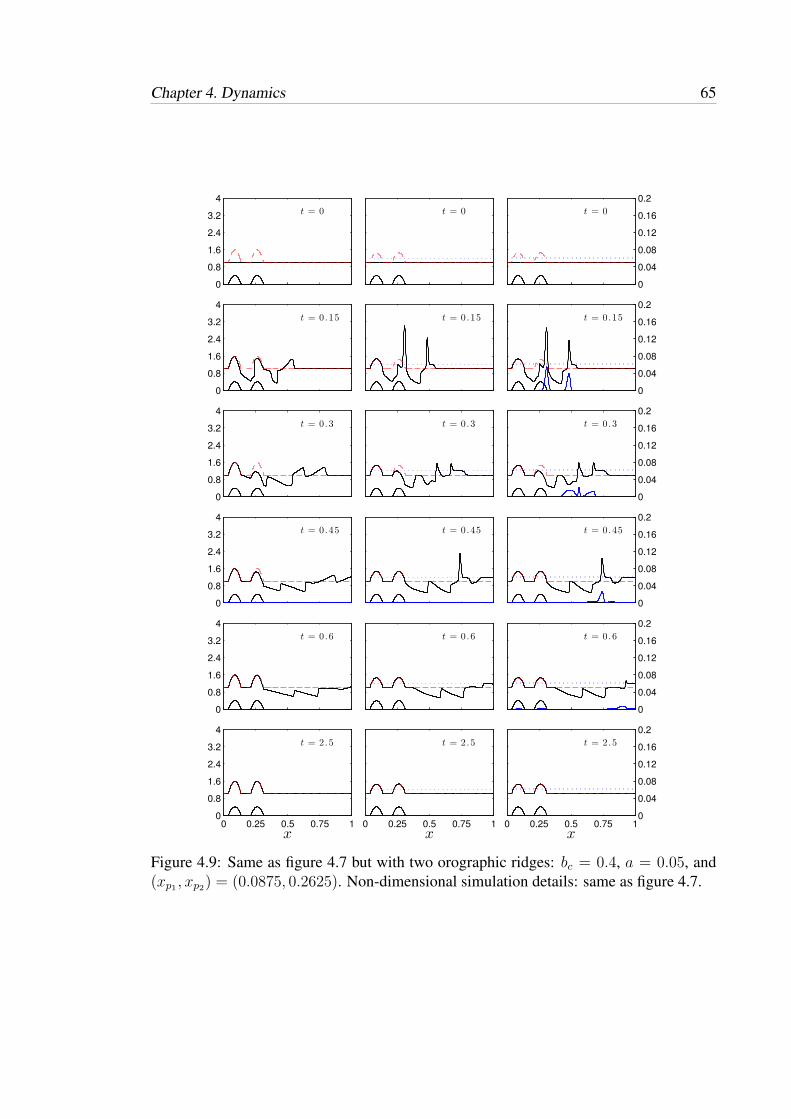
Chapter 4. Dynamics 65
0
0.8
1.6
2.4
3.2
4
t = 0 t = 0 t = 0
0
0.04
0.08
0.12
0.16
0.2
0
0.8
1.6
2.4
3.2
4
t = 0 .15 t = 0 .15 t = 0 .15
0
0.04
0.08
0.12
0.16
0.2
0
0.8
1.6
2.4
3.2
4
t = 0 .3 t = 0 .3 t = 0 .3
0
0.04
0.08
0.12
0.16
0.2
0
0.8
1.6
2.4
3.2
4
t = 0 .45 t = 0 .45 t = 0 .45
0
0.04
0.08
0.12
0.16
0.2
0
0.8
1.6
2.4
3.2
4
t = 0 .6 t = 0 .6 t = 0 .6
0
0.04
0.08
0.12
0.16
0.2
0 0.25 0.5 0.75 10
0.8
1.6
2.4
3.2
4
t = 2 .5
x0 0.25 0.5 0.75 1
t = 2 .5
x0 0.25 0.5 0.75 1
t = 2 .5
x
0
0.04
0.08
0.12
0.16
0.2
Figure 4.9: Same as figure 4.7 but with two orographic ridges: bc = 0.4, a = 0.05, and(xp1 , xp2) = (0.0875, 0.2625). Non-dimensional simulation details: same as figure 4.7.

66 Chapter 4. Dynamicst
x
h + b
0 0.25 0.5 0.75 10
0.2
0.4
0.6
0.8
1
< 1.25 3 >
x
−∂xu
0 0.25 0.5 0.75 1
< 0 5 >
x
r
0 0.25 0.5 0.75 1
0 0.04>
Figure 4.10: Same as figure 4.8 but with two orographic ridges. Non-dimensionalsimulation details: same as figure 4.7.
convective column as it propagates downstream from the ridge and slowly precipitates.
Such lee-side enhancement and propagation of deep convection downstream from a
ridge is a characteristic phenomenon of orographically-induced clouds [Houze Jr, 1993c].
Figure 4.8 plots Hr exceedance and wind convergence alongside r and, as with the
Rossby adjustment scenario, illustrates the conditions required for the production of rain.
Generating rain both requires and is proportional to positive wind convergence, so we
see more rain where this is greater. This relates to the physical argument put forward in
section 2.2 that rain is produced only when the fluid is rising and the amount of rain is
controlled by the strength of the updraft.
Figures 4.9 and 4.10 show corresponding results with two orographic ridges. Again,
the steady-state solution is achieved in all three cases, whilst the inclusion of a second
obstacle for the fluid introduces more complex dynamics and multiple regions of
convection and precipitation.
Semi-analytic steady state solutions for flow over topography
For standard shallow water flow, the exact steady state solution for the non-
dimensionalised equations is found by solving a third-order equation in h (4.4). For

Chapter 4. Dynamics 67
modRSW flow, an analytical equation for the steady state solution does not exist.
However, it is possible to derive a system of ordinary differential equations (ODEs) in
h and r and solve for their steady states. To facilitate this, we first combine (2.2a) with
2.2b) and 2.2d), yielding a system of equations for h, u, and r (similar to the model of
WC14; appendix A):
∂th+ ∂x(hu) = 0, (4.5a)
∂tu+ u∂xu+ ∂xΦ = 0, (4.5b)
∂tr + u∂xr + β∂xu+ αr = 0, (4.5c)
where Φ is given by equation (2.6). Steady-state solutions are found by considering time-
independent flow (∂t(·) = 0):
∂x(hu) = 0, (4.6a)
u∂xu+ ∂xΦ = 0, (4.6b)
u∂xr + β∂xu+ αr = 0, (4.6c)
The first of these steady-state equations gives immediately a solution of u in terms of h:
∂x(hu) = 0 =⇒ hu = K, for constant K =⇒ u =K
h, (4.7)
which is then substituted into the remaining equations, yielding a system of 2 ODEs to
solve for h and r. Using (4.7) and noting that:
∂xu = ∂x
(K
h
)= −K
h2∂xh, (4.8)

68 Chapter 4. Dynamics
the system in terms of h and r reads:
− K2
h3∂xh+ ∂xΦ = 0, (4.9a)
K
h∂xr −
K
h2β∂xh+ αr = 0. (4.9b)
A system of the formMMMXXX ′ = YYY is sought, whereXXX = (h, r)T , prime denotes derivative
with respect to x, and MMM ∈ R2×2, YYY ∈ R2 are given from the equations set. If MMM is
non-singular (and hence invertible), then we can solve XXX ′ = MMM−1YYY numerically for XXX
using, e.g., a simple finite difference scheme.
The system (4.9) is expanded as follows:
[− K2
h3+ g|Hc
]∂xh+
[c20
]∂xr = −
[g|Hc∂xb
], (4.10a)[K
h
]∂xr −
[Kh2β]∂xh = −
[αr], (4.10b)
where g|Hc = g if h + b ≤ Hc and zero otherwise and the terms in square brackets are
components ofMMM and YYY :
MMM =
−K2
h3+ g|Hc c20
−Kh2β K
h
, YYY =
−g|Hc∂xb−αr
. (4.11)
The β term (given in (2.4)) requires further manipulation; re-writing in terms of the
Heaviside function we have:
β = βΘ(−∂xu)Θ(h+ b−Hr)
= βΘ(K/h2∂xh)Θ(h+ b−Hr), using (4.7),
= βΘ(∂xh)Θ(h+ b−Hr). (4.12)
Thus, the system readsXXX ′ = f(XXX) where f(XXX) = MMM−1YYY and is solved using a forward

Chapter 4. Dynamics 69
Euler finite difference scheme: XXXj+1 = XXXj + 4xf(XXXj,XXXj−1). The value at j − 1 is
required to compute the Heaviside of the height gradient in (4.12); all other components
in f(XXX) = MMM−1YYY are evaluated using values at level j. To start marching through space,
note that XXX1 = XXX2, so that β = 0. Then proceed as usual for j ≥ 1. The solutions are
indicated in figures 4.7 and 4.9 (red dashed lines).
4.2 Summary
This chapter has investigated the dynamics of the modified shallow water model (2.2)
using the numerical methodology described in chapter 3. Classical numerical experiments
in shallow water theory, based on (i) the Rossby geostrophic adjustment problem (section
4.1.1) and (ii) non-rotating flow over topography (section 4.1.2), have been studied here
to illustrate the modified dynamics of the model. To highlight the response of the fluid
exceeding the threshold heights Hc < Hr, a hierarchy of model cases is employed and
the dynamics of each case is discussed with reference to the physical basis put forward in
chapter 2.
The model reduces exactly to the standard SWEs in non-convecting, non-precipitating
regions. It is clear from the model formulation in equations (2.2) – (2.4) that this should
be the case; the numerical model satisfies this, reproducing known shallow water results
in case I. The model also exhibits important aspects of convective-scale dynamics relating
to the disruption of large-scale balance principles which are of particular interest from a
DA perspective [Bannister, 2010]. The Rossby adjustment scenario clearly illustrates the
breakdown of geostrophic balance in the presence of convection and precipitation, while
the breakdown of hydrostatic balance is implicitly enforced by the modified pressure
(2.3) when the level of free convection Hc is exceeded. Furthermore, the experiments
simulated here have illustrated other features related to convecting and precipitating
weather systems, such as the initiation of daughter cells away from the parent cell by

70 Chapter 4. Dynamics
gravity wave propagation, and convection downstream from an orographic ridge.
Although based on the model of WC14, the absence of artificial diffusion terms from the
governing equations results in a mathematically cleaner formulation with conservation
of total mass (‘dry’ plus ‘rain’), and a markedly different dynamical behaviour emerges.
With the addition of rotation (and consequent Rossby adjustment dynamics) and analysis
of steady-state solutions for flow over topography, a rigorous investigation of the model’s
distinctive dynamics has been conducted in advance of its use in data assimilation
experiments.
This chapter brings the first part of this thesis, on the model and its dynamics, to
an end. The second part concerns data assimilation; the mathematical formulation of
the data assimilation problem (in particular Kalman filtering) is introduced in the next
chapter, along with practical considerations, before forecast–assimilation experiments are
conducted using the idealised fluid model in chapter 6.

71
Chapter 5
Data assimilation and ensembles:
background, theory, and practice
“In theory, there is no difference between theory and practice. But, in
practice, there is.” 1
Data assimilation (DA) is the process of combining limited and imperfect observations of
a system with an imperfect model to produce a more accurate and comprehensive estimate
of the current and future state of the modelled system as it evolves in space and time. A
successful assimilation algorithm takes into account any other useful information, such
as dynamical/physical constraints and knowledge of uncertainties, in producing the ‘best’
estimate of the state. This chapter introduces the mathematical formulation of the data
assimilation problem and the relevant background material for the next chapter. The basic
tools required to solve the DA problem are provided by filtering and estimation theory
(see, e.g., Jazwinski [2007]). In the context of NWP, Kalnay [2003] gives a concise
introduction to the DA problem and the various different solving techniques employed in
weather forecasting. The notation in this chapter follows that proposed by Ide et al. [1997]
1Jan L.A. van de Snepscheut (1953-1994), computer scientist.

72 Chapter 5. Data assimilation and ensembles: background, theory, and practice
where possible, with Houtekamer and Zhang [2016] also providing a concise notational
guide for the ensemble Kalman filter (section 5.3). There is somewhat of an overlap with
notation used in previous chapters; however, use of symbols and super/sub-scripts will be
defined herein independently of their use in previous chapters.
5.1 Overview of the classical DA problem
Consider an n–dimensional state vector x ∈ Rn, representing the (discrete) state of the
atmosphere. A prior estimate of the atmosphere typically comes from a forecast xf and
differs from the true state xt according to the the forecast error εf :
xf = xt + εf . (5.1)
Consider a p–dimensional vector y ∈ Rp of observations of the state of the atmosphere,
valid at the same time as the model state xf . In operational NWP, the state vector
contains the values of the prognostic variables at all model grid points. The number
of degrees of freedom of a forecast model, i.e., the value of n, is O(109) while the
number of observations is O(107) (see, e.g., Houtekamer and Zhang [2016]), so that n
is much greater than p. Furthermore, y is typically a very heterogeneous collection of
observations comprising numerous indirect and spatially–incomplete measurements of x.
The (nonlinear) observation operator H : Rn → Rp maps the state vector x from model
space to observation space:
y = H[xt] + εo, (5.2)
where εo ∈ Rp is the observational error, usually comprising instrumental and
representativeness errors. Representativity concerns the notion that the model is
not capable of representing some of the physical processes that can be seen in the
observations, owing to the resolution being too coarse, or simply the fact that some

Chapter 5. Data assimilation and ensembles: background, theory, and practice 73
processes are not being modelled at all (see, e.g., Janjic and Cohn [2006]). The error
term εo also accounts for errors in the observation operatorH.
The n–dimensional state vector x ∈ Rn is integrated forward in time using the nonlinear
(discretised) forecast modelM : Rn → Rn. Thus, the true state xt at a previous time ti−1
is related to the truth at the present time step ti via:
xt(ti) =M[xt(ti−1)] + ηi−1 (5.3)
where η ∈ Rn is the model error.
The quantification of uncertainty is a crucial part of any DA algorithm that seeks to
determine an optimal estimate of the model state vector. Thus, estimations of the error
statistics associated with the forecast and observations and their underlying probability
distributions are essential. The covariance between two random variables η1, η2 is defined
as:
cov(η1, η2) = 〈(η1 − 〈η1〉)(η2 − 〈η2〉)〉, (5.4)
where 〈·〉 is the expectation operator. In multivariate space, the representation (5.4) is
used to construct a covariance matrix which relates how vector components covary in
space. Thus, an error covariance matrix contains information about the magnitude of
errors and their correlations in space. It is assumed that the forecast and observation error
are unbiased (i.e., have zero mean) and are uncorrelated with each other:
〈εf〉 = 〈εo〉 = 0, and 〈εf (εo)T 〉 = 〈εo(εf )T 〉 = 0. (5.5)
The error covariance matrices for the forecast, observations, and model respectively are

74 Chapter 5. Data assimilation and ensembles: background, theory, and practice
given by:
Pf = 〈εf (εf )T 〉 ∈ Rn×n (5.6a)
R = 〈εo(εo)T 〉 ∈ Rp×p (5.6b)
Q = 〈ηηT 〉 ∈ Rn×n. (5.6c)
The goal of data assimilation is to estimate the state and uncertainty of the atmosphere
as accurately as possible by combining the forecast xf and observations y given their
respective uncertainties εf and εo. The ‘best’ estimate xa, called the analysis, is defined
by:
xa = xt + εa, (5.7)
where εa is the analysis error. Given the previous unbiased assumptions, εa is itself
unbiased, 〈εa〉 = 0, and the analysis error covariance is Pa = 〈εa(εa)T 〉 ∈ Rn×n.
A natural framework for tackling the DA problem is provided by Bayes’ theorem
(e.g., Wilks [2011]), which relates probability density functions (PDFs) of two random
variables A and B:
P (A|B) =P (B|A)P (A)
P (B). (5.8)
Let A be the event that x < xt < x + dx and B the event y < yt < y + dy, where yt is
the true observation. The aim is to find the state of the atmosphere x given observations
y, i.e., the posterior P (x|y). Applying Bayes’ (5.8) yields:
P (x|y) =P (y|x)P (x)
P (y), (5.9)
where P (y|x) is the conditional PDF of observations y given a state x (called the
likelihood and P (x) is the prior PDF of the forecast state. The prior PDF P (y) of the

Chapter 5. Data assimilation and ensembles: background, theory, and practice 75
observation vector is a normalising factor:
P (y) =
∫P (y|x′)P (x′)dx′, (5.10)
that ensures the posterior PDF is indeed a probability measure (i.e., the integral over all
probabilities is unity). The desired analysis state xa is the most probable state of the joint
PDF P (x|y)
Traditional DA methods are classified as either variational or sequential [Ide et al.,
1997]. Both approaches assume Gaussian statistics and produce an equivalent analysis
estimate. In practice however, this assumption rarely holds and the resulting posterior
estimate is a sub-optimal solution. Modern filtering techniques have been developed
which make no assumptions about the underlying distributions but a computationally–
tractable implementation for large problems such as NWP remains elusive.
There are typically two approaches to defining and computing the ‘best’ estimate, (i) the
‘maximum likelihood’ estimate and (ii) the ‘minimum variance’ estimate. The maximum
likelihood estimate (or maximum a posteriori (MAP) estimate) seeks the most likely x
and is determined by the mode of P (x|y). The minimum-variance estimate seeks to
minimise the analysis variance and is determined by the mean of P (x|y). Hence, for
Gaussian distributions (mean = mode), the two estimates are equivalent.
Assuming Gaussian forecast and observation errors, εf ∼ N (0,Pf ) and εo ∼ N (0,R),
the prior and likelihood are given by:
P (x) ∝ exp
[−1
2(x− xf )T (Pf )−1(x− xf )
], (5.11a)
P (y|x) ∝ exp
[−1
2(y −H[x])TR−1(y −H[x])
]. (5.11b)

76 Chapter 5. Data assimilation and ensembles: background, theory, and practice
Using (5.11) in (5.9) yields the posterior PDF:
P (x|y) ∝ exp
[−1
2(x− xf )T (Pf )−1(x− xf )
]× exp
[−1
2(y −H[x])TR−1(y −H[x])
]= exp
[−1
2
[(x− xf )T (Pf )−1(x− xf ) + (y −H[x])TR−1(y −H[x])
]]= exp [−J(x)] . (5.12)
The maximum probability (and corresponding analysis xa) occurs when x minimises the
cost function J(x). This function quantifies the distance between the analysis and the
forecast (weighted by the forecast error) and the analysis and the observations (weighted
by the observation error). Generally, the cost function J is minimized directly using
an iterative optimisation method that requires the computation of its gradient ∇J , a
linearised observation operator H (i.e., the Jacobian of H), and uses a prescribed static
forecast error covariance matrix. It provides the MAP analysis estimate as a weighted
linear combination of forecast and observation:
xa = xf +((Pf )−1 + HTR−1H
)−1HTR−1(y −H[xf ]). (5.13)
In the ‘minimum variance’ approach, the estimate is computed that minimises the mean
of the square error (“least–squares”) and is also a linear combination of forecast and
observation:
xa = xf + K(y −H[xf ]). (5.14)
The observation departure y−H[xf ] is weighted by a matrix K ∈ Rn×p and the problem
is solved by seeking the optimum elemental weights in K that yield the analysis with
the minimum variance. The resulting matrix is called the Kalman gain and combines

Chapter 5. Data assimilation and ensembles: background, theory, and practice 77
information from the forecast and observation error covariances:
K = PfHT (HPfHT + R)−1, (5.15)
and yields the Best Linear Unbiased Estimate (BLUE; see, e.g., Kalnay [2003]) as well
as an expression for the analysis error covariance:
Pa = (I−KH)Pf . (5.16)
This procedure is also known as ‘Optimal Interpolation’. It is useful to interpret this
weighting procedure in one dimension (i.e., n = p = 1) with a state x ∈ R and a single
observation y ∈ R of the same variable (so that H = 1), with forecast error variance
σ2f and observation error variance σ2
o . The Kalman gain (5.15) weights the observation
increments by the forecast error variance normalised by the total error variance:
K =σ2f
σ2f + σ2
o
. (5.17)
If the forecast is very accurate compared to the observations (σ2f σ2
o), then K→ 0 and
the forecast xf dominates. On the other hand, if the forecast is of a much lower quality
than the observations (σ2f σ2
o), then K→ 1 and the observation y is given the maximum
weight. From a different perspective, if for some reason the variance of the forecast is
underestimated (i.e., there is over-confidence in its skill), then valid observations may not
have the expected influence when producing the analysis estimate.
The Kalman gain plays an analogous role in higher dimensions (i.e., n > 1): the optimal
weight is given by the forecast error covariance normalised by the total error covariance
taking into account the different model and observation spaces in which the respective
covariances are expressed. However, it plays a far greater role in higher dimensions as it
contains information on spatial correlations between variables via the error covariance

78 Chapter 5. Data assimilation and ensembles: background, theory, and practice
matrices. The structure of Pf in particular has a profound impact on the quality of
the analysis estimate: variances on its diagonal estimate the confidence in the forecast
state while off-diagonal elements allow the spreading of information in space between
variables.
The importance of Pf is evident in the following example with n = 2 and p = 1.
Consider a state vector x = (x1, x2)T ∈ R2 with forecast error variances σ2
f1 and σ2f2
and covariances c, and a direct measurement y ∈ R of x1 with error variance σ2o . Then
the matrices of interest are:
Pf =
σ2f1 c
c σ2f2
, R = σ2o , H = H =
[1 0
], (5.18)
and so the Kalman gain equals:
K = PfHT (HPfHT + R)−1
=
σ2f1 c
c σ2f2
1
0
[1 0]σ2
f1 c
c σ2f2
1
0
+ σ2o
−1
=1
σ2f1 + σ2
o
σ2f1
c
. (5.19)
The resulting analysis increment is a vector proportional to the first column of Pf :
xa − xf =y − xf1σ2f1 + σ2
o
σ2f1
c
, (5.20)
and shows clearly how an unobserved state component (in this case x2) is updated via
the off-diagonal covariances of Pf . Accordingly, a misspecified Pf results in incorrect
updates and can have a very detrimental impact on the analysis estimate.
Using the Sherman-Morrison-Woodbury formula [Sherman and Morrison, 1950], the

Chapter 5. Data assimilation and ensembles: background, theory, and practice 79
Kalman gain matrix can be rewritten:
K = PfHT (HPfHT + R)−1 =((Pf )−1 + HTR−1H
)−1HTR−1, (5.21)
and it becomes clear that the analysis estimates (5.13, 5.14) derived using the two
different approaches are indeed equivalent. Although arriving at the same estimate,
the two approaches are algorithmically very different and yield two distinct frameworks
for solving the DA problem. The solution derived by considering the MAP estimate
and minimising a cost function is known as three–dimensional variational assimilation
(3DVAR), while the minimum-variance estimate obtained via the Kalman gain is called
Optimal Interpolation (OI). The choice of method depends on the size of the problem
in hand; historically NWP has favoured variational methods but modern variants of the
Kalman filter (which uses the OI equations) are becoming more popular in practice.
5.2 Kalman Filtering
The Kalman Filter (KF; Kalman [1960]; Kalman and Bucy [1961]) is a sequential method
in which a linear model is integrated forward in time from an initial analysis state estimate
and, whenever observations are available, they are used to reinitialise the model before
the integration continues. However, NWP involves solving nonlinear partial differential
equations describing atmospheric motion on many scales, and so a linear DA method
such as the standard KF is wholly inadequate. In an attempt to overcome this deficiency,
advances in nonlinear Kalman filtering have led to schemes which at least partially
capture some of the nonlinearity, including the Extended Kalman Filter (EKF; in which
the forecast and observation models can be nonlinear) and the Ensemble Kalman Filter
(EnKF; which uses an ensemble of nonlinear model integrations). Here, I outline the
concepts and formulation of the traditional KF and its modern variants, and highlight
some crucial points for its numerical implementation.

80 Chapter 5. Data assimilation and ensembles: background, theory, and practice
Kalman filtering can be described in a two-step process: a ‘forecast’ step advances the
model state and its corresponding error statistics, followed by an ‘analysis’ step which
assimilates the observations in a way to produce an optimal estimate of the state and
reinitialise the model. This sequence is repeated in a loop when observations become
available. To start the loop, prior knowledge of the state is needed. Here, this is
assumed to come from a previous forecast, which provides the state vector itself and
some corresponding statistical information (e.g., correlation/covariance structure).
5.2.1 The forecast step
The goal of the KF (and indeed any DA scheme) is to provide the best estimate of the
true state xt given all the information available. This information typically consists
of a prior forecast (or an analysis obtained in the previous DA cycle) and sequential
observations/measurements of the modelled system. The following formulation assumes
nonlinear model dynamics, and so derives the EKF. For the standard KF, M is a linear
operator (or ‘state transition matrix’). Given the analysis xa at time ti−1, the forecast state
xf at the next time step ti is determined by the (imperfect) model dynamics:
xfi =Mi−1[xai−1]. (5.22)
The error covariance matrix associated with the model state vector x is given by P. For
the analysis and forecast respectively, this is defined as:
Pa = 〈(xa − xt)(xa − xt)T 〉 = 〈εa(εa)T 〉, (5.23a)
Pf = 〈(xf − xt)(xf − xt)T 〉 = 〈εf (εf )T 〉, (5.23b)
where the difference between truth and analysis (forecast) is defined as the analysis
(forecast) error: xa = xt + εa (xf = xt + εf ). It is assumed that these errors are
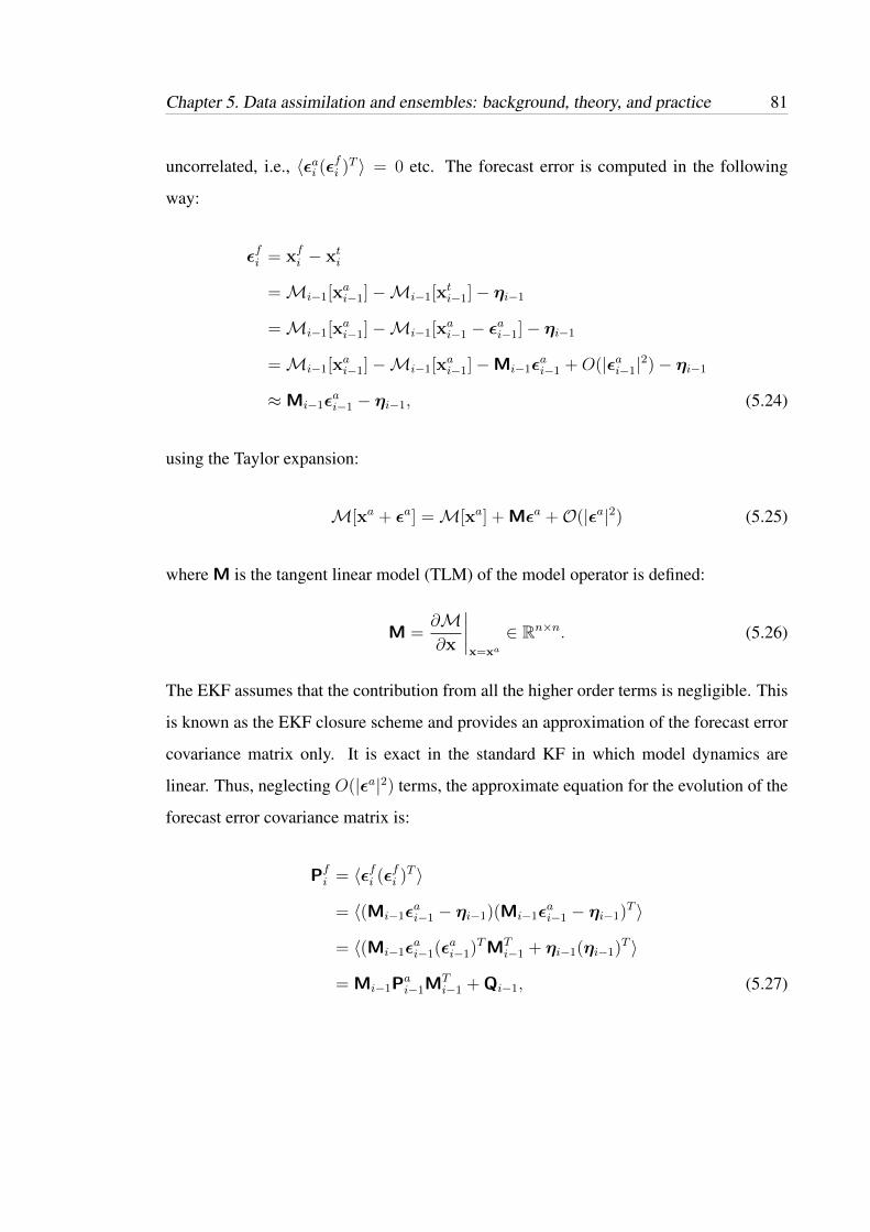
Chapter 5. Data assimilation and ensembles: background, theory, and practice 81
uncorrelated, i.e., 〈εai (εfi )T 〉 = 0 etc. The forecast error is computed in the following
way:
εfi = xfi − xti
=Mi−1[xai−1]−Mi−1[x
ti−1]− ηi−1
=Mi−1[xai−1]−Mi−1[x
ai−1 − εai−1]− ηi−1
=Mi−1[xai−1]−Mi−1[x
ai−1]−Mi−1ε
ai−1 +O(|εai−1|2)− ηi−1
≈Mi−1εai−1 − ηi−1, (5.24)
using the Taylor expansion:
M[xa + εa] =M[xa] + Mεa +O(|εa|2) (5.25)
where M is the tangent linear model (TLM) of the model operator is defined:
M =∂M∂x
∣∣∣∣x=xa
∈ Rn×n. (5.26)
The EKF assumes that the contribution from all the higher order terms is negligible. This
is known as the EKF closure scheme and provides an approximation of the forecast error
covariance matrix only. It is exact in the standard KF in which model dynamics are
linear. Thus, neglecting O(|εa|2) terms, the approximate equation for the evolution of the
forecast error covariance matrix is:
Pfi = 〈εfi (εfi )T 〉
= 〈(Mi−1εai−1 − ηi−1)(Mi−1ε
ai−1 − ηi−1)T 〉
= 〈(Mi−1εai−1(ε
ai−1)
TMTi−1 + ηi−1(ηi−1)
T 〉
= Mi−1Pai−1M
Ti−1 + Qi−1, (5.27)

82 Chapter 5. Data assimilation and ensembles: background, theory, and practice
where Qi−1 = 〈ηi−1ηTi−1〉 from (5.6c). The model forecast (5.22) and its corresponding
error covariance matrix (5.27) constitute the forecast step of the EKF:
xfi =Mi−1[xai−1]
Pfi = Mi−1Pai−1M
Ti−1 + Qi−1
(5.28a)
(5.28b)
Note that the previous analysis state xai−1 and its error covariance matrix Pai−1 are assumed
known (‘prior information’) from a previous cycle (see figure 5.1).
5.2.2 The analysis step
In the analysis step, observational information available at time ti is merged with previous
information carried forward by the forecast step in a way that gives the ‘best’ estimate of
the true state. This estimate, namely the analysis at time ti, is obtained by adding an
optimally weighted observational increment to the forecast state:
xai = xfi + Kidi (5.29)
where Ki is the optimal weight and di is the observational increment (known as
the ‘innovation’), defined as the difference between the observation and forecast in
observation space:
di = yi −Hi[xfi ]. (5.30)
The matrix Ki is the Kalman gain matrix:
Ki = PfiHTi (HiP
fiH
Ti + Ri)
−1, (5.31)
a time-dependent extension of the weight matrix (5.15) of the ‘Optimal Interpolation’
equations, which give the ‘best linear unbiased estimation’ for the analysis xa. It

Chapter 5. Data assimilation and ensembles: background, theory, and practice 83
weights the innovation d according to the ratio between forecast and observational error
covariances, where H is the TLM of the (nonlinear) observation operatorH:
H =∂H∂x
∣∣∣∣x=xf
∈ Rp×n. (5.32)
As with the model dynamics, the standard KF assumes a linear observation operator. The
Kalman gain is also used to update the analysis error covariance matrix Pa. Using the
Taylor expansion ofH about xf :
Hi[xti] = Hi[x
fi − ε
fi ] = Hi[x
fi ]−Hiε
fi +O(|εf |2) (5.33)
with higher-order error terms ignored, the analysis error is given by:
εai = xai − xti
= xfi + Ki(yi −Hi[xfi ])− xti
= xfi − xti + Ki(yi −Hi[xti] +Hi[x
ti]−Hi[x
fi ])
= εfi + Ki(εoi −Hix
fi )
= (I−KiHi)εfi + Kiε
oi . (5.34)
Then the analysis error covariance matrix (5.23a) is given by:
Pai =⟨(
(I−KiHi)εfi + Kiε
oi
)((I−KiHi)ε
fi + Kiε
oi
)T⟩= (I−KiHi)〈(εfi )(ε
fi )T 〉(I−KiHi)
T + Ki〈(εoi )(εoi )T 〉KTi
= (I−KiHi)Pfi (I−KiHi)
T + KiRiKTi . (5.35)

84 Chapter 5. Data assimilation and ensembles: background, theory, and practice
Finally, rewriting equation (5.31) so that Ki(HiPfiH
Ti + Ri)K
Ti = PfiH
Ti K
Ti , a concise
expression is obtained for the Kalman-updated analysis error covariance matrix:
Pai = Pfi −KiHiPfi − PfiH
Ti K
Ti + KiHiP
fiH
Ti K
Ti + KiRiK
Ti
= Pfi −KiHiPfi
= (I−KiHi)Pfi . (5.36)
This expression (5.36) and the update equation (5.29) complete the analysis step of the
KF:
xai = xfi + PfiHTi (HiP
fiH
Ti + Ri)
−1di
where di = yi −Hi[xfi ]
Pai = (I−KiHi)Pfi
(5.37a)
(5.37b)
(5.37c)
Once complete, the model is reinitialised with the updated analysis and the loop continues
forward as observations are made available. This Kalman filtering algorithm is illustrated
in figure 5.1.
5.2.3 Summary
The general formulation of the KF has been outlined here as a sequential data assimilation
technique which merges observational data and a model forecast in a way that produces
a best estimate of the model state. The outcome is optimal in the ‘best linear unbiased
estimation’ and ‘cost function minimisation’ sense [Kalnay, 2003].
In the standard KF, the forecast modelM and forward observation operatorH are linear,
while one or both of the models are nonlinear in the EKF. An important theorem from
filtering theory for the linear KF states that if the dynamical system comprising imperfect
state propagation and imperfect measurements is uniformly completely observable and
uniformly completely controllable, then the KF is uniformly asymptotically stable

Chapter 5. Data assimilation and ensembles: background, theory, and practice 85
Prior knowledgeof state
xa(ti−1)Pa(ti−1)
Forecast step:using model dynamicsM,
TLM M, and model error Q.
xf (ti)Pf (ti)
Reinitialise model:go to next time step
Analysis step:add weighted innovation
to forecast
xa(ti)Pa(ti)
Available observations:y(ti), R(ti)
Output estimate ofstate: xa(ti) and
uncertainty Pa(ti)
Figure 5.1: A schematic diagram illustrating the general formulation of the KF. Thefiltering technique starts with some given prior information and then continues in cycleswith the availability of observations.
(see, e.g., Jazwinski [2007]). Observability refers to the amount of observation
information and takes into account the propagation of this information with the model.
Controllability refers to the plausibility of nudging the system to the correct solution by
applying appropriate increments. Uniform asymptotic stability implies that, for bounded
observation errors, the errors in the output will remain bounded regardless of the initial
data. This means that even with an unstable modelM, the KF will stabilise the system.
A major drawback of the EKF in NWP is the huge computational cost involved in
propagating the forecast error covariance matrices Pf . This is equivalent to dim(x)
forward model integrations, where dim(x) is of order 109. This is extremely prohibitive
and is the major reason why the EKF is not a tractable algorithm for operational forecast–
assimilation systems. Another problem of the EKF is the use of the approximate
closure scheme in (5.27), in which third- and higher-order moments in the forecast
error covariance equation are discarded. Evensen [2003] notes that this linearisation is

86 Chapter 5. Data assimilation and ensembles: background, theory, and practice
often invalid in a number of applications, e.g., in Evensen [1992] the linear evolution
of Pf in an ocean model leads to an unbounded linear instability. Miller et al. [1994]
noted that estimated solutions were only tolerable in a short time interval and proposed
a generalisation of the EKF which extended the covariance evolution to include third-
and fourth-order moments. Although this leads to improvements in the estimation, it still
remains a computationally expensive approximation.
Recent developments in the NWP and DA community have led to techniques which
approximate and update the forecast error covariance matrix in a computationally
tractable manner and attempt to capture the nonlinearity associated with atmospheric
modelling. The main obstacle hindering applications with a high-dimensional
atmospheric forecast model is obtaining an appropriate low-dimensional approximation
of the forecast error covariance matrix for a feasible implementation on a computational
platform. The use of random ensembles currently seems to be the most practical way to
address the issue.
5.3 The Ensemble Kalman Filter
The Ensemble Kalman Filter (EnKF) was introduced by Evensen [1994] and combines
Kalman Filter theory with Monte Carlo estimation methods. It follows the same
conceptual framework of the standard KF and EKF, outlined in the previous section,
but differs in that it uses Monte Carlo methods to estimate the error covariances of
the forecast error. In doing so, it provides an approximation to the time-dependent
forecast error covariance matrix Pf without the need of the tangent linear model M in
the forecast step (see equation (5.27)). It implicitly treats the errors as Gaussian by
its reliance on the mean and covariance, which completely characterise the Gaussian
distribution. In combination with other techniques (addressed in section 5.5), it provides
an approximation to the Kalman-Bucy filter [Kalman, 1960; Kalman and Bucy, 1961])

Chapter 5. Data assimilation and ensembles: background, theory, and practice 87
that is feasible for operational atmospheric DA problems; additionally, it provides an
ensemble of initial conditions that can be used in an ensemble prediction system.
The EnKF is relatively simple to implement and much more affordable computationally
than the EKF. Furthermore, it does not use any linearisations for the forward integration of
the forecast error covariance, thereby including the full effects of nonlinear dynamics. By
providing flow-dependent estimates of the background error from the nonlinear model,
the EnKF is better suited to adapting to current observations than the EKF (which uses
linear flow-dependency) and 3DVAR (which assumes static background error).
Since its first application in Evensen [1994], there have been numerous important
contributions to its development, notably by Burgers et al. [1998], Houtekamer and
Mitchell [1998], Evensen and Van Leeuwen [2000], and Houtekamer and Mitchell [2001].
Evensen [2003] reviews the important results of these studies and gives a comprehensive
overview of the formulation and implementation of the EnKF. Meng and Zhang [2011]
and Houtekamer and Zhang [2016] provide more recent reviews and cover issues relating
to high-resolution ensemble-based Kalman filtering.
5.3.1 Basic equations
In the following, subscripts are reserved for indexing ensemble members only, not time
as in the previous section. For an N–member ensemble, the j th member xj (j = 1, .., N )
is integrated forward via (possibly a perturbed realisation of) the forecast modelMj:
xfj (ti) =Mj[xaj (ti−1)], j = 1, ..., N, (5.38)

88 Chapter 5. Data assimilation and ensembles: background, theory, and practice
and the update (analysis) is performed using a randomly perturbed vector of observations
yj:
xaj (ti) = xfj (ti) + K(yj −H[xfj (ti)]), (5.39a)
K = PfHT (HPfHT + R)−1, (5.39b)
where K and the matrices within are at time ti. This time-dependence is now implicitly
assumed and no longer indexed. The reason for using perturbed observations is addressed
in the following section. As is typical in the Monte Carlo approach to forecasting, the
best estimate of the state is given by the ensemble mean:
x =1
N
N∑j=1
xj. (5.40)
State error covariance matrices in the standard Kalman filter are defined in terms of a
(usually unknown) truth state, as in (5.23a, 5.23b), and must accordingly be modelled in
some way. In the EnKF, the error covariance matrix is approximated using an ensemble
of states (i.e., an ensemble of nonlinear model integrations):
P ' Pe =1
N − 1
N∑j=1
(xj − x)(xj − x)T
=N
N − 1(x− x)(x− x)T (5.41)
where the overline denotes an average over the ensemble. In this set-up, errors are defined
as perturbations from the ensemble mean rather than the truth and the forecast error is
characterised by covariance matrix. It should be noted that in an EnKF it is not necessary
to compute the full covariance matrix Pf in model state space, which is prohibitively large
if n is of order O(109). Instead, when computing the Kalman gain in (5.39), one can use

Chapter 5. Data assimilation and ensembles: background, theory, and practice 89
ensemble approximations to PfHT andHPfHT [Houtekamer and Mitchell, 2001]:
PfHT =1
N − 1
N∑j=1
(xfj − xf )(H[xfj ]−H[xf ])T , (5.42a)
HPHT =1
N − 1
N∑j=1
(H[xfj ]−H[xf ])(H[xfj ]−H[xf ])T , (5.42b)
where xf is the forecast ensemble mean (5.40) and we define the mean of the forecast
ensemble in observation space:
H[xf ] =1
N
N∑j=1
H[xfj ]. (5.43)
In this way, the full non–linear observation operator H is used in the update. To
summarise the basic EnKF equations:
Forecast: xfj (ti) =Mj[xaj (ti−1)], j = 1, ..., N,
Analysis: xaj (ti) = xfj (ti) + K(yj −H[xfj (ti)]),
K = PfHT (HPfHT + R)−1.
(5.44a)
(5.44b)
(5.44c)
5.3.2 The stochastic filter: treatment of observations
After the first implementation of an EnKF by Evensen [1994], Burgers et al. [1998] and
Houtekamer and Mitchell [1998] noted that for a completely consistent analysis scheme
the observations should be treated as random variables, i.e., random perturbations should
be added to the observations which are sampled from a distribution with mean equal to
the ‘first-guess’ observation y and covariance R. If this is not the case, the EnKF scheme
results in an updated ensemble with a variance which is too low.

90 Chapter 5. Data assimilation and ensembles: background, theory, and practice
Without perturbed observations
To illustrate this, consider first an EnKF cycle (i.e., a forecast followed by an analysis
update) in which the (same) observation vector y is assimilated into all ensemble
forecasts. Assume also for simplicity that the observation operator is linear, H = H.
The forecast step is:
xfj (ti) =Mj[xaj (ti−1)], j = 1, ...N, (5.45)
and Pfe is given by (5.41) at time ti. Each ensemble member is then updated using the
Kalman gain matrix (5.31) with Pf replaced by Pfe , all at time ti:
xaj = xfj + PfeHT (HPfeH
T + R)−1︸ ︷︷ ︸=:Ke
(y −Hxfj ). (5.46)
The analysis mean is given by:
xa =1
N
N∑j=1
xaj =1
N
N∑j=1
xfj + Ke(y −Hxfj )
,
=1
N
N∑j=1
xfj + Ke(y −H1
N
N∑j=1
xfj ),
= xf + Ke(y −Hxf ). (5.47)
The final step is to evaluate the analysis ensemble error covariance Pae given by the
definition (5.41). From (5.46) and (5.47):
xaj − xa = xfj − xf + Ke(y −Hxfj )−Ke(y −Hxf ),
= xfj − xf −KeH(xfj − xf ),
= (IN −KeH)(xfj − xf ), (5.48)
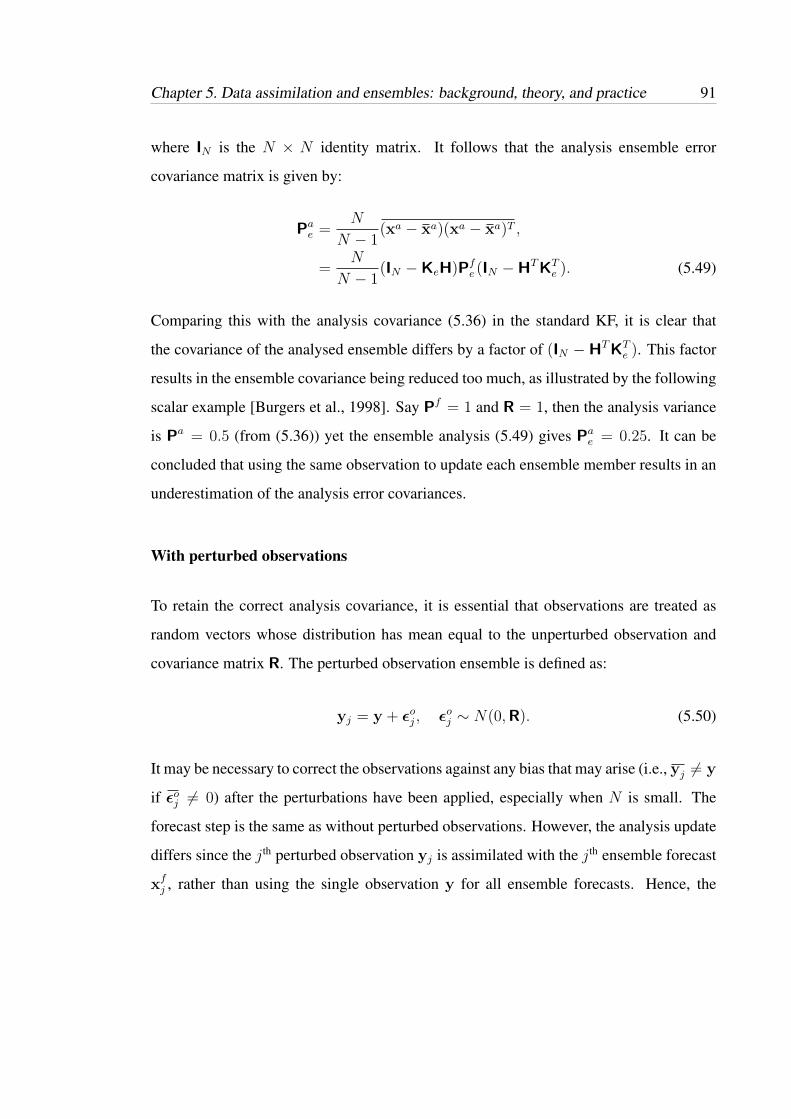
Chapter 5. Data assimilation and ensembles: background, theory, and practice 91
where IN is the N × N identity matrix. It follows that the analysis ensemble error
covariance matrix is given by:
Pae =N
N − 1(xa − xa)(xa − xa)T ,
=N
N − 1(IN −KeH)Pfe (IN −HTKT
e ). (5.49)
Comparing this with the analysis covariance (5.36) in the standard KF, it is clear that
the covariance of the analysed ensemble differs by a factor of (IN −HTKTe ). This factor
results in the ensemble covariance being reduced too much, as illustrated by the following
scalar example [Burgers et al., 1998]. Say Pf = 1 and R = 1, then the analysis variance
is Pa = 0.5 (from (5.36)) yet the ensemble analysis (5.49) gives Pae = 0.25. It can be
concluded that using the same observation to update each ensemble member results in an
underestimation of the analysis error covariances.
With perturbed observations
To retain the correct analysis covariance, it is essential that observations are treated as
random vectors whose distribution has mean equal to the unperturbed observation and
covariance matrix R. The perturbed observation ensemble is defined as:
yj = y + εoj , εoj ∼ N(0,R). (5.50)
It may be necessary to correct the observations against any bias that may arise (i.e., yj 6= y
if εoj 6= 0) after the perturbations have been applied, especially when N is small. The
forecast step is the same as without perturbed observations. However, the analysis update
differs since the j th perturbed observation yj is assimilated with the j th ensemble forecast
xfj , rather than using the single observation y for all ensemble forecasts. Hence, the

92 Chapter 5. Data assimilation and ensembles: background, theory, and practice
analysis step reads:
xaj = xfj + Ke(yj −Hxfj ), (5.51)
where Ke = PfeHT (HPfeH
T + R)−1, (5.52)
with analysis mean given by (5.47). Errors are given by perturbations from the ensemble
mean:
xaj − xa = xfj − xf + Ke(yj −Hxfj )−Ke(y −Hxf ),
= xfj − xf + Ke(yj − y)−KeH(xfj − xf ),
= (IN −KeH)(xfj − xf ) + Ke(yj − y). (5.53)
and the analysis ensemble error covariance matrix is given by:
Pae =N
N − 1(xa − xa)(xa − xa)T ,
=N
N − 1(IN −KeH)Pfe (IN −HTKT
e ) + KeReKTe ,
=N
N − 1(IN −KeH)Pfe . (5.54)
This expression is the result obtained previously (5.36) in the standard KF analysis scheme
with the covariance matrices replaced by their ensemble representations. It is clear that
perturbed observations are required to get the observation error covariance R into the
expression of analysis covariance and that by treating observations as random vectors
there is correspondence between the standard KF and EnKF in both the forecast and
analysis step. Indeed, the EnKF with perturbed observations in the limit of infinite
ensemble size gives the same result in the calculation of the analysis as the KF and EKF
[Evensen, 2003]. A schematic for the EnKF algorithm is shown in figure 5.2.

Chapter 5. Data assimilation and ensembles: background, theory, and practice 93
5.3.3 Matrix formulation
It is useful to consider the matrix representation when implementing the EnKF analysis
scheme. Bold type face x is used to denote a full state vector in Rn only and is indexed by
the ensemble member j. Where there are 2 subscripts xkj , k = 1, ..., n indexes the state
vector component and j = 1, ..., N indexes the ensemble member. The N independent
ensemble members are collated into an n×N matrix, defined as the ensemble state matrix:
X =(x1 x2 · · · xN
)=
x11 x12 · · · x1N
x21 x22 · · · x2N...
......
xn1 xn2 · · · xnN
∈ Rn×N , (5.55)
with superscript f and a for the forecast and analysis ensemble matrix respectively. Define
the ensemble mean matrix X as the product of X with 1N ∈ RN×N , a square matrix with
all elements are equal to 1/N :
X = X1N =1
N
N∑j=1
x1jN∑j=1
x1j · · ·N∑j=1
x1j
N∑j=1
x2jN∑j=1
x2j · · ·N∑j=1
x2j
......
...N∑j=1
xnjN∑j=1
xnj · · ·N∑j=1
xnj
=⇒ X =
x1 x1 · · · x1
x2 x2 · · · x2...
......
xn xn · · · xn
∈ Rn×N . (5.56)
Thus, the ensemble mean matrix stores the ensemble mean state x ∈ Rn, repeated in each
column. Ensemble perturbations (or displacements about the centre of mass) are defined

94 Chapter 5. Data assimilation and ensembles: background, theory, and practice
as the difference between each ensemble member and the ensemble mean: x′j = xj − x.
In matrix form:
X′ = X− X =(x′1 x′2 · · · x′N
)
=
x11 − x1 x12 − x1 · · · x1N − x1x21 − x2 x22 − x2 · · · x2N − x2
......
...
xn1 − xn xn2 − xn · · · xnN − xn
∈ Rn×N , (5.57)
Thus, the ensemble error covariance matrix can be defined (from (5.41)):
Pe =1
N − 1
N∑j=1
(xj − x)(xj − x)T
=1
N − 1
((x1 − x)(x1 − x)T + · · ·+ (xN − x)(xN − x)T
)=
1
N − 1
(x′1 x′2 · · · x′N
)(x′1 x′2 · · · x′N
)T=
1
N − 1X′(X′)T ∈ Rn×n, (5.58)
with appropriate superscripts for analysis and forecast. Diagonal entries are the variances
and off-diagonal entries are the covariances between each component in the state vector
x: X′(X′)T =
N∑j=1
(x1j − x1)2N∑j=1
(x1j − x1)(x2j − x2) · · ·N∑j=1
(x1j − x1)(xnj − xn)
N∑j=1
(x2j − x2)(x1j − x1)N∑j=1
(x2j − x2)2 · · ·N∑j=1
(x2j − x2)(xnj − xn)
......
...N∑j=1
(xnj − xn)(x1j − x1)N∑j=1
(xnj − xn)(x2j − x2) · · ·N∑j=1
(xnj − xn)2
.
(5.59)

Chapter 5. Data assimilation and ensembles: background, theory, and practice 95
Similarly, perturbed observations are assembled into the columns of the p×N matrix Υ:
Υ =(y1 y2 · · · yN
)∈ Rp×N . (5.60)
Using the matrices defined in this way, the analysis equation for the EnKF is written:
Xa = Xf + Ke(Υ−H[Xf ])
where Ke = PfeHT (HPfeHT + R)−1, (5.61)
andH[Xf ] is shorthand for applyingH to each column of Xf in turn. The ensemble mean
analysis can also be expressed in the matrix representation:
Xa = Xa1N = Xf1N + Ke(Υ−H[Xf ])1N
= Xf + Ke(Υ−H[Xf ]), (5.62)
and the analysis error covariance matrix follows directly from (5.58):
Pae =1
N − 1X′a(X′a)T . (5.63)
5.3.4 Summary
The forecast and analysis scheme for the EnKF has been derived here and shown to
maintain the same structure as the standard KF. The EnKF was proposed by Evensen
[1994] as a Monte Carlo alternative to the deterministic EKF. It uses an ensemble of
forecasts to estimate and evolve flow-dependent background error covariances which
are required to compute the Kalman gain in the analysis step. If the same observations
are used to update each ensemble member, there is a systematic underestimation of the
analysis error covariances. However, by treating the observations as random variables

96 Chapter 5. Data assimilation and ensembles: background, theory, and practice
Generate initialensemble using, e.g.,
ensemble of initial states
xaj (ti−1)xa(ti−1)
Forecast step: updateeach member individuallyusing model dynamicsM
xfj (ti)
xf (ti)Pfe (ti)
Reinitialise model:go to next time step
Analysis step: addweighted innovation withperturbed obs. to forecast
xaj (ti)xa(ti)
Perturb obs.:yj(ti) = y(ti) + εoj
Available observations:y(ti), R(ti)
Output estimate ofstate xa(ti) and
error Pae(ti)
Figure 5.2: A schematic diagram illustrating the general formulation of the EnKF. TheEnKF forecast and update equations with perturbed observations are structurally identicalto those of the traditional and extended KF.
and assimilating an ensemble of stochastically perturbed observations with correct error
statistics, this problem is corrected [Burgers et al., 1998; Houtekamer and Mitchell,
1998]. Moreover, it has been shown [Mandel et al., 2011] that, with linear forecast
and observation models and in the limit of large ensemble size, the EnKF converges in
probability to the KF.
Unlike the EKF, there is no need for linearisations in the propagation of forecast error
statistics, and consequently the effects of nonlinear dynamics in the forecast model
are included. Moreover, the computationally expensive tangent linear model M and

Chapter 5. Data assimilation and ensembles: background, theory, and practice 97
its adjoint MT are not required, making the EnKF easier to implement in practical
applications with high-dimensional state vectors. A useful artefact of the EnKF is the
automatic computation of a random sample of analysis states (and the corresponding
error distribution) which can be used as initial conditions for an ensemble prediction
system. Ensemble generation for NWP is a key area of research which has greatly
benefited both to and from the development of ensemble DA methods. An ensemble of
perturbations obtained from the analysis error statistics is by construction intrinsically
suited to ensemble prediction initialisation, i.e., the DA scheme produces “realistic”
perturbations, in the sense that the initial perturbations reflect the statistics evolved by
the underlying dynamics via the estimated analysis uncertainty [Kalnay, 2003].
5.4 Other filters
Numerous other ensemble-based filters exist, some of which are sufficiently developed to
be operational, others which still require further advancement before potential usage in an
NWP setting. Some of the most popular flavours are briefly discussed here, but since the
stochastic EnKF is the method employed in this thesis, further details are omitted. Reich
and Cotter [2015] provide an excellent summary of numerous linear and nonlinear filters.
5.4.1 Deterministic filters
Treating observations as random variables leads to a stochastically formed analysis
ensemble and subsequent estimate of analysis errors. This stochastic scheme produces
asymptotically correct analysis estimates for large enough ensemble size, yet it inevitably
introduces further sampling errors (one source of sampling errors is already present
through estimation of the forecast error covariances). These additional sampling errors
arise due to the Monte Carlo simulation of observations and subsequent estimation of

98 Chapter 5. Data assimilation and ensembles: background, theory, and practice
observation error covariances (i.e., treating observations as random variables). Increased
sampling errors can lead to biased analysis error covariance estimates [Tippett et al.,
2003]. This has motivated the development and use of deterministic (or ‘square root’)
filters that form the analysis ensemble deterministically, thereby removing sampling
errors associated with perturbed observations. Since it avoids the impact of spurious
correlations from perturbed observations, the deterministic filter can achieve a comparable
performance as a corresponding stochastic filter with a smaller total ensemble size
[Mitchell and Houtekamer, 2009]. However, it has also been shown [Lawson and Hansen,
2004] that, without the regular introduction of random forcing, the deterministic filter
can develop highly non-Gaussian distributions and subsequently degrade the KF solution
which assumes Gaussian statistics. As such, it may be considered less robust than the
stochastic EnKF [Houtekamer and Zhang, 2016].
5.4.2 Ensemble transform filters
The ensemble transform Kalman filter (ETKF) is a suboptimal KF that uses a transform
to obtain rapidly the forecast error covariance matrices [Bishop et al., 2001]. In doing so,
it lends itself to an efficient implementation in an operational setting. The local ETKF
(LETKF; Hunt et al. [2007]) merges the transform filter with the Local Ensemble Kalman
Filter [Ott et al., 2004], and has also been developed with computational efficiency on
massively parallel computers in mind. The Met Office uses an LETKF to initialise
their ensemble prediction system [Bowler et al., 2008, 2009] and other operational
configurations are employed by the Italian Meteorological Service (CNMCA; Bonavita
et al. [2010]) and Deutsche Wetter Dienst (DWD; Schraff et al. [2016]). The Japanese
Meteorological Agency (JMA) and ECMWF have developed an LETKF for research
purposes.

Chapter 5. Data assimilation and ensembles: background, theory, and practice 99
5.4.3 Nonlinear filters
Nonlinear data assimilation, in which no assumptions are made about the underlying
probability distributions, is receiving a lot of attention in the geosciences [van Leeuwen,
2010]. This is unsurprising; given that higher resolution models include more small-
scale processes and more complex and indirect observations require highly nonlinear
observation operators, the data assimilation problem is becoming more and more
nonlinear.
Nonlinear filters are nothing new (e.g., Anderson and Anderson [1999]; Bengtsson et al.
[2003] and the particle filter has been applied in the geosciences [Van Leeuwen, 2009].
However, these filters are known to be extremely inefficient due to the so–called ‘curse
of dimensionality’, which states that the number of particles (i.e., ensemble members)
required scales exponentially with the state dimension [Snyder et al., 2008; Bengtsson
et al., 2008; Van Leeuwen, 2009]. This renders particle filters wholly unsuitable for the
NWP problem in their current form, but recent variants have attempted to address the
curse of dimensionality and have been applied to high dimensional systems (e.g., Ades
and Van Leeuwen [2013, 2015]). Nonetheless, NWP is an extremely high dimensional
problem and a great deal of progress and further research is required before fully nonlinear
data assimilation is plausible in an operational system.
5.5 Issues in ensemble-based Kalman filtering
Monte-Carlo ensemble forecasts attempt to sample the true PDF of the atmosphere
starting from a finite number of initial random perturbations [Epstein, 1969; Leith, 1974].
The ensemble provides a discrete estimate of this distribution; the mean (‘first moment’)
yields the Best Linear Unbiased Estimate of the future state, while the covariance (‘second
moment’), of the ensemble exemplifies the uncertainty in the ensemble mean forecast

100 Chapter 5. Data assimilation and ensembles: background, theory, and practice
[Murphy, 1988]. These finite sample estimates are known to converge slowly and
considerably undersample the true PDF when the number of degrees of freedom is large
[Stephenson and Doblas-Reyes, 2000]. In the context of NWP, the computational cost of
integrating the forecast model M limits the size of the ensemble N used operationally,
which is typically O(10− 100), much smaller than the number of degrees of freedom of
the model n = O(109). Consequently, all ensemble DA schemes suffer from sampling
error as N n.
The efficiency and effectiveness of the EnKF algorithm depends on myriad factors, almost
all of which stem from this undersampling due to the small ensemble size [Houtekamer
and Mitchell, 1998]. The ensemble is used to estimate the forecast error covariance
matrix which has a profound impact on the success in any data assimilation problem.
As such, special techniques are necessary to counter the limited ensemble size and obtain
good filter behaviour. Issues in ensemble-based Kalman filtering are well documented
and comprehensive reviews of the problems and alleviating techniques can be found in
Ehrendorfer [2007] and Houtekamer and Zhang [2016]. The rest of this section discusses
three of the main issues pertinent for this thesis in more detail and summarises other points
of concern for practical implementation of the EnKF.
5.5.1 The rank problem and ensemble subspace
The forecast error covariance matrix has dimension n × n and to calculate Pf in the
original (E)KF equations requires n model integrations. This is clearly prohibitively large
for the NWP problem in which n = O(109), but if it were attainable it would provide
n different directions (i.e., eigenvectors of Pf ) in the model’s phase space on which to
project the observational information. However, an EnKF system withN members covers
a subspace with at most N − 1 directions which is evidently much restricted compared
with the full space. This means that the p observations must be mapped onto a limited
number of directions [Lorenc, 2003].

Chapter 5. Data assimilation and ensembles: background, theory, and practice 101
To illustrate this mathematically, consider the Kalman update equation (5.39) for the
analysis increment of ensemble member j, rewritten as a linear transform:
xaj − xfj = Pfevj, where vj = HT (HPfeHT + R)−1(yj −H[xfj ]), (5.64)
and recall that Pfe is defined as the outer product of forecast deviations from the mean
(5.58). Then it is apparent that the analysis increments lie in the subspace of the ensemble:
xaj − xfj =1
N − 1(Xf )′((Xf )′)Tvj =
1
N − 1(Xf )′vj (5.65)
for vj = ((Xf )′)Tvj . This means that the analysis increments are constrained to lie in the
span of the columns of (Xf )′, even if observations indicate otherwise.
The rank problem, namely that N n and N p, manifests the sampling issue
in the EnKF and is one of the main differences compared to the original KF theory
[Houtekamer and Zhang, 2016]. The small number of directions and lack of information
of the full model space leads to an ensemble which does not sufficiently sample the space
and is potentially underspread. Rank deficiency of Pf , and how this is dealt with, is a
crucial aspect when the EnKF is implemented in practice. Concerning idealised forecast-
assimilation experiments with the simplified fluid model, the rank problem is less severe
since the model space is much reduced (n = O(100− 1000)) and depends very much on
the observing system.
5.5.2 Maintaining ensemble spread: the need for inflation
A well-configured and sufficiently spread ensemble is key to providing an adequate
estimation of forecast error in the EnKF. The ensemble spread should be comparable to the
root mean square error of the ensemble mean if the filter is to perform adequately. It is well
known that ensembles exhibit insufficient spread due to undersampling [Houtekamer and

102 Chapter 5. Data assimilation and ensembles: background, theory, and practice
Mitchell, 1998]. Indeed, globally-averaged spread values in an ECMWF ensemble DA
system have been found to be half the size of the corresponding forecast error [Bonavita
et al., 2012], and Houtekamer and Zhang [2016] note that other ensemble-based DA
studies reveal that in general only about a quarter of the error variance of the ensemble
mean is explained by the ensemble.
Insufficient ensemble spread can lead to ‘inbreeding’ [Houtekamer and Mitchell, 1998],
a phenomenon in which the analysis error covariances are consistently underestimated,
leading to ever–smaller ensemble spread. Underestimating ensemble error is akin to the
EnKF placing too much confidence in the accuracy of the ensembles at the expense
of the observations, which may be more faithful to reality. This causes a feedback
cycle in which ever more trust is placed on the forecasts (hence the term inbreeding)
and the observations are eventually ignored altogether. Once the ensemble spread
collapses due to ever-smaller error estimates, the ensemble mean diverges completely
from the observations. To maintain sufficient spread and prevent this ‘filter divergence’
due to undersampling, so-called covariance inflation techniques have been developed.
Broadly speaking, inflation methods are either multiplicative or additive (although more
specialised adaptive algorithms exist) and increase the ensemble spread to a desired level.
The concept of additive inflation originates in the standard KF theory. When the forecast
error covariance matrix is evolved in the forecast step (5.27), the model error covariance
terms contribute to the updated forecast errors. In a similar vein, additive inflation
comprises adding random Gaussian perturbations ηj ∼ N (0, γaQQQ) during the forecast
step:
xj(ti) =M(xj(ti−1)) + ηj, j = 1, ..., N (5.66)
where the forecast–model error matrix QQQ is prescribed from some knowledge of the
modelling system and γa is a tunable parameter controlling the overall magnitude of the
sample perturbations. How one best defines QQQ is an open question - ideally it should be
constructed using flow-dependent perturbations [Hamill and Whitaker, 2011] but is often

Chapter 5. Data assimilation and ensembles: background, theory, and practice 103
a static matrix developed offline from historical analysis increments. Additive inflation
does not try to represent the model error explicitly, but acts in some sense as a lower bound
for the forecast error, thus preventing filter divergence. Moreover, the addition of random
Gaussian perturbations can counteract the non-Gaussian higher moments nonlinear error
growth may have generated in the forecast step, and since the optimal EnKF solution
assumes Gaussian distributions, this is expected to benefit the quality of the analysis
estimate [Houtekamer and Zhang, 2016]. However, adding random Gaussian noise may
also mask useful covariance information pertaining to the model dynamics.
The simplest and most popular form of covariance inflation is multiplicative [Anderson
and Anderson, 1999], a ‘catch-all’ method which artificially inflates the ensemble
perturbations:
xj ← x + γm(xj − x), γm > 1, (5.67)
where γm is a factor tuned to give the desired spread. Multiplicative inflation tends to work
well when γm remains fairly close to one [Houtekamer and Zhang, 2016], however larger
values are often required in operational NWP systems. Care should be taken when larger
values are used as the repeated application may prompt unbounded covariance growth in
data–sparse areas [Anderson, 2009].
Both additive and multiplicative inflation are somewhat ad hoc in their approach in
that factors γa,m require tuning on an individual basis. Two common adaptive inflation
methods aim to standardise the process: ‘Relaxation To Prior Perturbation’ (RTPP; Zhang
et al. [2004]) and ‘Relaxation To Prior Spread’ (RTPS; Whitaker and Hamill [2012]).
It is widely accepted that inflation techniques are crucial for maintaining sufficient
ensemble spread and satisfactory filter performance; typically, a combination of additive,
multiplicative, and adaptive methods are used in practice. However, it is should be noted
that the alterations in the ensemble trajectories due to inflation dilute the impact of flow–
dependent statistics developed in the EnKF.

104 Chapter 5. Data assimilation and ensembles: background, theory, and practice
5.5.3 Spurious correlations: the need for localisation
The rank problem means that correlations present in the error covariance matrices are also
subject to sampling error. This is manifest as spurious correlations in the forecast error
covariance, i.e., unphysical correlations between components in the state vector (usually
at long distances) due to sampling noise. For example, two components of x whose
true correlation (“signal”) is negligible may have a non-negligible spurious correlation
(“noise”) according to Pf . Since observations influence the analysis estimate via Pf ,
spurious correlations can lead to components of the state vector being falsely updated by
a distant and/or physically irrelevant observation. Thus, if the noise is greater than the
signal in Pf (as is the case at long distances for N n), the analysis update is degraded
[Hamill et al., 2001]. The sampling errors essentially make the long distance correlations
untrustworthy, and the effects of the resulting noise may outweigh improvements that DA
has achieved elsewhere in the spatial domain.
Localisation is a technique that attempts to prevent the analysis estimate being degraded
by spurious correlations by cutting off long range correlations in the error covariance
matrix [Hamill et al., 2001; Houtekamer and Mitchell, 2001; Whitaker and Hamill, 2002].
The intuition behind localisation relates directly to the rank problem and limitations of
the ensemble subspace. By splitting the full assimilation problem into several smaller
‘local’ problems, the N ensemble members only have to span the (smaller) local space,
effectively increasing the rank of the problem [Hamill et al., 2001; Oke et al., 2007]. The
increase in rank is apparent in the eigenvalue spectrum of the localised covariance matrix
[Petrie, 2012] and implies that there are more degrees of freedom for assimilating the
observations, resulting in a greater observational influence on the final analysis estimate
[Ehrendorfer, 2007]. It is widely accepted that the severity of the rank problem in NWP
and heterogeneity of the observing system means ensemble-based DA methods are only
feasible when used in conjunction with localisation [Hamill et al., 2001; Ehrendorfer,
2007; Anderson, 2012; Houtekamer and Zhang, 2016].

Chapter 5. Data assimilation and ensembles: background, theory, and practice 105
Localisation is usually achieved by multiplying the elements of the forecast error
covariance matrix with elements of a carefully chosen covariance taper matrix ρ that
reduces correlations as a function of distance. In matrix operations, this comprises
elementwise multiplication and is achieved using the Schur (or Hadamard) product
[Schur, 1911]:
(A B)ij = AijBij, (5.68)
for two matrices A and B of the same dimension and i, j indexing the row and
column number respectively. Entries of the covariance taper matrix ρ are calculated
using a correlation function % with compact support (i.e., non-zero in local region, zero
everywhere else), resulting in a localised forecast error covariance matrix Pfloc = ρ Pf .
Several properties of the Schur product, reviewed by Horn [1990], make it a desirable
choice for implementing localisation. Three of the most important theorems concerning
localisation are repeated here (see Horn [1990] for further details and proofs):
1. IfA,B are square matrices that are positive semi-definite, then so isA B.
2. If B is a strictly positive square matrix and A is a positive semi-definite matrix
of the same size with all its main diagonal entries positive, then A B is strictly
positive definite.
3. Let A be a positive semi-definite correlation matrix (i.e., all diagonal entries equal
to 1) and let B be a positive semi-definite matrix of the same size (say, m by m).
Suppose that their eigenvalues λi(A) and λi(B) are each ordered decreasingly such
that λ1 ≥ λ2 ≥ · · · ≥ λm ≥ 0. Then:
k∑i=1
λi(A B) ≤k∑i=1
λi(B), k = 1, 2, ...,m. (5.69)
It follows from theorem 1 that the Schur product of two covariance matrices is also a
covariance matrix. Theorem 2 implies that even though Pf is rank-deficient, if a positive

106 Chapter 5. Data assimilation and ensembles: background, theory, and practice
definite taper matrix is chosen (and Pf has positive variances which is typically the case)
then the localised covariance ρ Pf has full rank. Finally, it follows from theorem 3 that:
Tr(ρ Pf ) ≤ Tr(Pf ). (5.70)
This means that, although localisation can solve the problem of rank-deficiency, it does
not increase the overall variance, and so is typically used in combination with covariance
inflation (section 5.5.2).
The most common choice for the localising function %, and the one taken in this thesis,
is the so-called Gaspari-Cohn function, a fifth-order piecewise rational function (Gaspari
and Cohn [1999]; equation 4.10). It has similar shape to a half-Gaussian and depends
on a single length-scale parameter (Lloc; see figure 5.3). The correlations are filtered out
gradually and suppressed completely beyond a certain distance Lloc (due to the compact
support), leading to an observation having zero influence there.
Implementing localisation remains a fairly ad hoc procedure and is very much specific
to the problem and flavour of EnKF used. Ideally, model-space localisation Pf ←
ρ Pf should be used [Houtekamer and Zhang, 2016], however this is unfeasible due
to the dimension of Pf . However, localisation can be implemented via the ensemble
approximations (5.42), ρ(PfHT ) and ˜ρ(HPfHT ). The choice of length-scale is clearly
crucial and should reflect the signal-to-noise ratio as the distance increases, attempting to
maintain true correlations until the effects of sampling error dominate. Flowerdew [2015]
has attempted to introduce a systematic approach to localisation based on minimising
analysis variance given a fixed ensemble size, but a standardised technique for such
complex systems with an array of heterogeneous observations remains elusive. As such,
a degree of tuning and experimentation is required to find the optimum length-scale for
an individual forecast-assimilation system.
As with inflation techniques, it should be noted that replacing Pf with its localised form

Chapter 5. Data assimilation and ensembles: background, theory, and practice 107
0 50 100 150 200x
0.0
0.2
0.4
0.6
0.8
1.0
Lloc=50
Lloc=80
Lloc=200
Lloc=∞
Figure 5.3: Example Gaspari-Cohn functions % for different length-scales Lloc as afunction of distance x. Here, x is the number of equally-spaced grid points away from theobservation location at x = 0. Lloc = ∞ implies no localisation (cyan line); the smallerLloc, the tighter the localisation. The number of grid points relates to the experiments inchapter 6.
represents quite a departure from the KF theory, and therefore a localised EnKF does
not possess a number of properties intrinsic in the standard EnKF. For example, the
resulting analysis increments (5.64) will no longer be completely in the space spanned
by the forecast ensembles and may lead to states that are not completely dynamically
consistent [Oke et al., 2007]. Consequently, forecasts initialised from the analyses and
and subsequent cycles may exhibit a rapid adjustment (‘initialisation shock’, see, e.g.,
Daley [1993]) due to the inconsistencies associated with the analysis.

108 Chapter 5. Data assimilation and ensembles: background, theory, and practice
5.6 Interpreting an ensemble-based forecast-assimilation
system
5.6.1 Error vs. spread
An ideal ensemble is expected to have the same magnitude of ensemble spread as the
root mean square error of its mean at the same lead time in order to adequately represent
the full uncertainty in the forecast [Stephenson and Doblas-Reyes, 2000]. The root mean
square error of the ensemble mean is defined as:
RMSE =
√√√√ 1
n
n∑k=1
(xk − xtk)2 , where xk =1
N
N∑j=1
xkj, (5.71)
and xtk is the kth component of the true state vector xt. A natural measure of the typical
spread of the ensemble is the root mean squared dispersion:
SPR =
√√√√ 1
N − 1
N∑j=1
1
n
n∑k=1
(xkj − xk)2 ≡√
1
nTr(P) . (5.72)
where P is the error covariance matrix (as in (5.59)). The ‘spread vs. RMS error’ statistics
provide a simple but relevant diagnostic on the suitability of the generated ensemble in
the EnKF.
5.6.2 Observation influence diagnostic
The update equation for the Kalman filter provides an optimal analysis state xa by
combining observations y with some background (prior) information xf , usually from a

Chapter 5. Data assimilation and ensembles: background, theory, and practice 109
previous forecast. This analysis estimate is the optimal generalised least squares solution:
xa = xf + K(y −Hxf )
= Ky + (I−KH)xf , (5.73)
where K = PfHT (HPfHT + R)−1 contains error information of the observations and
prior to accordingly weight both pieces of information. The projection of the analysis
estimate into observation space, calculated by left-multiplying (5.73) by the observation
operator H:
y = Hxa = HKy + (I−HK)Hxf , (5.74)
is the sum of observations and the background in observation space weighted by the
matrices HK and I−HK respectively.
The influence matrix S, developed in ordinary least squares regression analysis, monitors
the influence of individual data sources on the analysis estimate. In this case, data sources
are observations and the background state, and the influence matrix provides a measure
of the overall impact of observations/background state on the analysis. The analysis
sensitivity with respect to observations is defined by:
S =∂y
∂y= HK. (5.75)
Similarly, the analysis sensitivity with respect to the backround (all in observation space)
is given by:∂y
∂(Hxf )= I−HK = I− S. (5.76)
The global average observation influence diagnostic is defined as:
OID =Tr(S)
p, where p = dim(y), (5.77)
and provides a norm for quantifying the overall influence of observations on the analysis

110 Chapter 5. Data assimilation and ensembles: background, theory, and practice
estimate. Cardinali et al. [2004] have applied this diagnostic to the ECMWF global
NWP model and found an observation influence of 0.18, suggesting that the global
average observation influence is quite low compared to that of the forecast. That is,
the analysis estimate primarily comes from the prior forecast, adjusted slightly towards
the observations. However, it should be noted that the prior forecast estimate contains
observational information from previous analysis cycles.
5.6.3 Continuous Ranked Probability Score
In the EnKF, a well–configured ensemble is crucial to good performance as it is used to
the estimate flow–dependent forecast–error covariances. Spread and RMSE are a good
first check for an adequately performing ensemble, but it would be useful to have a
tool that focuses on the entire permissible range of outcomes, i.e., the full distribution
provided by the ensemble. The Continuous Ranked Probability Score (CRPS; Matheson
and Winkler [1976]; Hersbach [2000]; Hamill et al. [2001]; Jolliffe and Stephenson
[2003]; Brocker [2012]) verifies the reliability of an ensemble for scalar quantities, and is
a popular verification tool for probabilistic forecasts. Reliability measures the degree to
which forecast probabilities agree with outcome frequencies. It is a negatively–oriented
scoring rule that assigns a numerical score (zero being perfect) to probabilistic forecasts
and form attractive summary measures of predictive performance. A key feature of the
CRPS is that it generalizes the absolute error to which it reduces if the forecast is a
point measure (i.e., deterministic forecast). Thus, it is a valid metric for evaluating both
probabilistic and deterministic forecasts, and so can be used to compare the performance
of two conceptually different forecasts.
The challenge for diagnosis of probabilistic forecasts is that the forecast takes the form
of a distribution function F (or density P ) whereas the observations (or true state) are
point–valued. The CRPS expresses the “distance” between a forecast F and true value
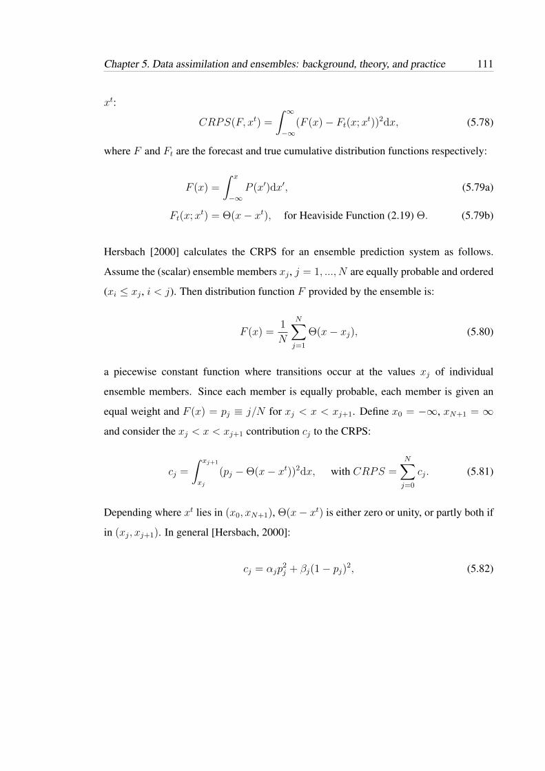
Chapter 5. Data assimilation and ensembles: background, theory, and practice 111
xt:
CRPS(F, xt) =
∫ ∞−∞
(F (x)− Ft(x;xt))2dx, (5.78)
where F and Ft are the forecast and true cumulative distribution functions respectively:
F (x) =
∫ x
−∞P (x′)dx′, (5.79a)
Ft(x;xt) = Θ(x− xt), for Heaviside Function (2.19) Θ. (5.79b)
Hersbach [2000] calculates the CRPS for an ensemble prediction system as follows.
Assume the (scalar) ensemble members xj , j = 1, ..., N are equally probable and ordered
(xi ≤ xj , i < j). Then distribution function F provided by the ensemble is:
F (x) =1
N
N∑j=1
Θ(x− xj), (5.80)
a piecewise constant function where transitions occur at the values xj of individual
ensemble members. Since each member is equally probable, each member is given an
equal weight and F (x) = pj ≡ j/N for xj < x < xj+1. Define x0 = −∞, xN+1 = ∞
and consider the xj < x < xj+1 contribution cj to the CRPS:
cj =
∫ xj+1
xj
(pj −Θ(x− xt))2dx, with CRPS =N∑j=0
cj. (5.81)
Depending where xt lies in (x0, xN+1), Θ(x− xt) is either zero or unity, or partly both if
in (xj, xj+1). In general [Hersbach, 2000]:
cj = αjp2j + βj(1− pj)2, (5.82)

112 Chapter 5. Data assimilation and ensembles: background, theory, and practice
where:
αj =
xj+1 − xj,
xt − xj,
0,
βj =
0, if xj+1 < xt,
xj+1 − xt, if xj < xt < xj+1,
xj+1 − xj if xj > xt.
(5.83)
It should be noted that outliers can contribute significantly to the CRPS: if the true value
does not lie in the ensemble range then extra weight is given to the penalising terms.
Also, it is defined for scalar quantities x, and so is calculated for each element of the state
vector x, e.g., for the idealised fluid model (2.2) the CRPS is calculated for each variable
at each grid point.
5.6.4 Error-growth rates
The error–doubling time Td of a forecast-assimilation system is the time taken for the
error E of a finite perturbation (produced by the analysis increment) at time T0 to double:
E(Td)
E(T0)= 2, (5.84)
where E is some error norm (usually taken to be the RMSE). The error–doubling time
is expected to fluctuate somewhat between variables (since certain variables behave more
nonlinearly than others) and is controlled by the ‘dynamics of the day’. However, by
averaging over a number of staggered forecasts covering a range of dynamics and initial
perturbations, the mean error–doubling time of the system can be estimated. For global
NWP, Buizza [2010] found a doubling time of 1.28 days for the Northern Hemisphere
forecast error. Errors in high-resolution NWP grow faster than in the global case due to
the strong nonlinearities at convective scales. Thus, in order to be relevant for convective-
scale NWP, the idealised forecast-assimilation system should be tuned to give a mean

Chapter 5. Data assimilation and ensembles: background, theory, and practice 113
error–doubling time on the order of hours rather than a day. Moist convection severely
limits mesoscale predictability [Zhang et al., 2003], and for limited–area cloud–resolving
models, the mean error–doubling time has been found to be around 4 hours [Hohenegger
and Schar, 2007].

114 Chapter 5. Data assimilation and ensembles: background, theory, and practice

115
Chapter 6
Idealised DA experiments
“The frontier of data assimilation is at the high spatial and temporal
resolution, where we have rapidly developing precipitating systems with
complex dynamics”1
As described in chapter 2 and shown in chapter 4, the modified shallow water model is
able to simulate some fundamental dynamical processes of convecting and precipitating
weather systems, thus suggesting that it is a suitable candidate for investigating DA
algorithms at convective scales. In this chapter, the assimilation techniques described
in chapter 5 are applied to the idealised fluid model to demonstrate this suitability
further. An exploration of the model’s distinctive dynamics should be considered a
necessary but not sufficient qualification for its suitability. By demonstrating a well-
tuned forecast-assimilation system that exhibits characteristics of high-resolution NWP,
one can be confident that the model is indeed a useful tool for inexpensive yet relevant
DA experiments (e.g., Inverarity [2015]).
Achieving a meaningful and interesting experimental set-up is more nuanced than simply
interfacing a model with an assimilation algorithm. It requires careful consideration of
1 Houtekamer and Zhang [2016]

116 Chapter 6. Idealised DA experiments
the ‘real–life’ problem at hand, in this case convective–scale NWP and DA, and should
attempt to mimic certain attributes of the whole system, not just the dynamical aspects.
The first section of this chapter introduces the ‘twin model environment’, in which
idealised experiments are performed, and sets up the basic framework of the forecast–
assimilation system. In practice, operational forecast–assimilation systems require a great
deal of tuning in order to perform optimally, taking into account all facets of the forecast
model, the observing system, and the assimilation algorithm. Accordingly, the process of
developing and arriving at a well–tuned system deserves attention in an idealised setting.
This process is conveyed in the following sections before focussing on aspects of a single
experiment in greater detail. The results of this exploratory investigation, together with
the dynamical analysis in chapter 4, indicate that the model provides an interesting testbed
for DA research in the presence of convection and precipitation.
6.1 Twin model environment
Data assimilation research using idealised models is primarily carried out in a so–called
‘twin’ experiment setting, whereby the same computational model is used to generate
a ‘nature’ run (which acts as a surrogate truth) and the forecasts. If the forecasts are
generated using exactly the same model integration as the nature run, the resulting DA
experiments are said to be carried out in a perfect model setting. On the other hand, in an
imperfect model scenario, forecasts are generated using a different model configuration,
e.g., with misspecified model parameters or at a coarser spatial resolution.
The nature run is a single long integration of the numerical model and is a proxy for
the true evolving physical system. It is the principal difference between idealised and
operational DA experiments and its function is twofold. First, it is used to produce
pseudo-observations of the physical system, which are then assimilated into the forecast
model. These pseudo-observations (also known as synthetic observations) are generated
Chapter 6. Idealised DA experiments 117
by applying the observation operator H to the state vector from the nature run xt and
adding random samples from a specified observational error distribution. Second, it
provides a verifying state with which to compare the forecast and analysis estimates
and thus quantify the errors in each. The configuration of the model and assimilation
algorithm employed in this chapter is described here.
6.1.1 Setting up an idealised forecast–assimilation system
Model: dynamics
Motivated by the experiments with orography in chapter 4 (in particular figure 4.9),
supercritical flow over topography is considered for the experiments herein with non-
dimensional parameters Ro = ∞ and Fr = 1.1. The topography is defined to be a
superposition of sinusoids in a sub-domain and zero elsewhere:
b =
3∑i=1
bi, for xp < x < xp + 0.5;
0, elsewhere;
(6.1)
and bi = Ai(1 + cos
(2π(ki(x− xp)− 0.5)
))(6.2)
where xp = 0.1, k = 2, 4, 6, A = 0.1, 0.05, 0.1. Given a non-zero initial velocity and
periodic boundary conditions (3.12), this ‘collection of hills’ (see top panels in figure 6.1)
generates varied and complex dynamics (including gravity-wave excitation) without the
need for external forcing or an imposed mean wind field. Periodic BCs mean that waves
that leave the domain wrap around again, and so the flow remains energetic; this keeps
the flow moving and dynamically interesting without further forcing.
Given the Froude and Rossby number, potential characteristic scales of the dynamics
can be analysed and, where possible, likened to high-resolution NWP. Note that infinite

118 Chapter 6. Idealised DA experiments
0 0.1 0.2 0.3 0.4 0.5 0.6 0.7 0.8 0.9 10
2
4
6
8
t=1
x
h(x
,t)
0 0.1 0.2 0.3 0.4 0.5 0.6 0.7 0.8 0.9 10
0.5
1
1.5
2
x
u(x
,t)
0 0.1 0.2 0.3 0.4 0.5 0.6 0.7 0.8 0.9 10
0.02
0.04
0.06
0.08
0.1
x
r(x,t)
(a) Forecast xf : Nel = 200
0 0.1 0.2 0.3 0.4 0.5 0.6 0.7 0.8 0.9 10
2
4
6
8
t=1
x
h(x
,t)
0 0.1 0.2 0.3 0.4 0.5 0.6 0.7 0.8 0.9 10
0.5
1
1.5
2
x
u(x
,t)
0 0.1 0.2 0.3 0.4 0.5 0.6 0.7 0.8 0.9 10
0.02
0.04
0.06
0.08
0.1
x
r(x,t)
(b) Nature xt: Nel = 800
Figure 6.1: Snapshot of model variables h (top), u (middle), and r (bottom) from (a)the forecast model and (b) the nature run. The forecast trajectory is smoother andexhibits ‘under-resolved’ convection and precipitation while the nature run has sharper‘resolved’ features and is a proxy for the truth. The thick black line in the top panels isthe topography (eq. 6.1), the red dotted lines are the threshold heights.
Rossby number implies non-rotating flow, and therefore zero transverse velocity v (if it
is initially zero). Consider a fixed length of domain L0 = 500 km and velocity-scale
V0 ∼ 20 ms−1, implying a time-scale T0 ∼ 25000 seconds (∼ 6.94... hours). Thus, one
hour is equal to 0.144 non-dimensional time units. A Froude number Fr = 1.1 implies
gH0 ∼ 330 m2s−2.
Model: defining forecast and nature
Current high-resolution NWP models are operating with a horizontal gridsize on the order
of one kilometre. For example, the Met Office’s UKV model has a gridsize of 1.5 km
and MOGREPS-UK ensemble runs at 2.2 km [Tang et al., 2013; Bowler et al., 2008];
Chapter 6. Idealised DA experiments 119
the Deutsche Wetter Dienst’s COSMO-DE model has a 2.8 km horizontal grid spacing
[Baldauf et al., 2011]. Running models at this resolution means that convection is resolved
explicitly (albeit poorly) and yields more realistic–looking precipitation fields [Lean et al.,
2008]. With this in mind, a forecast grid spacing of ∼ 2.5km is imposed for the idealised
model. Thus, given that the length of domain is L0 ∼ 500 km, the computational grid has
Nel = 200 elements and the total number of degrees of freedom of the forecast model is
n = 600 (note that hv is removed from the integration since flow is non-rotating).
Despite the improved representation of clouds and precipitation in models with gridsize
O(1km), it is widely recognised that convection is still under-resolved and does not exhibit
many aspects of observed convection [Tang et al., 2013]. To reflect this, an imperfect
model scenario is employed in which the nature run is generated at a (four times) finer
resolution than the forecast model, i.e., Nel = 800 for the nature run. This is the only
difference compared to the model configuration used for the forecast integrations. An
example trajectory of both forecast and nature at a given time is shown in figure 6.1;
conceptually, the basic data assimilation problem can be summarised using this figure:
adjust the forecast (6.1a) using pseudo-observations of the “truth” in order to provide a
better estimate of the nature run (6.1b).
Assimilation: experimental set-up and algorithm
The EnKF and its variants have been extensively investigated with different models at
different scales (see Meng and Zhang [2011] for a review on high-resolution ensemble-
based DA and Houtekamer and Zhang [2016] for a general EnKF review). There are
strong arguments for ensemble-based algorithms at convective scales, primarily the use
of the ensemble for approximating the forecast error covariances. Having flow-dependent
error statistics is crucial at finer scales where nonlinear error growth proliferates. Here, the
‘perturbed-observation’ (stochastic) EnKF is chosen to be the algorithm for the idealised
forecast-assimilation system, owing to its straightforward implementation and robustness.

120 Chapter 6. Idealised DA experiments
The state vector is defined x = (h, u, r)T ∈ Rn rather than in terms of flux variables
x = (h, hu, hr)T ∈ Rn used in the model integration. Thus, the model operator M,
namely the numerical scheme derived in chapter 3, acts on x and before passing the
model state x to the analysis step, it is transformed via a mapping Ψ to the state vector:
x = Ψ(x). This simply maps h to h, hu to u, and hr to r.
The analysis update frequency is fixed to be one hour, and ensemble size is N = 40
(comparable to operational convective-scale systems, e.g., Schraff et al. [2016]). All
variables are observed directly (hence the observation operator is linear, H = H) with
specified error σσσ = (σh, σu, σr) and density ∆y (e.g., observe every 20 gridcells ∼ 50km
on forecast grid). This observing system and filter configuration (i.e., localisation length-
scale and inflation factors) should be tuned to give an experimental set-up relevant for
convective-scale NWP. Exactly what this entails is addressed in section 6.1.2.
A compact algorithm for one complete cycle (forecast plus analysis) of the EnKF is
summarised here, to be read loosely with figure 5.2.
1. FORECAST STEP:
(a) To start the cycle, one requires a prescribed ensemble of initial conditions xicj .
That is, for i = 1:
xfj (t1) =M[xicj ], j = 1, ..., N. (6.3)
(b) At later times, the forecast uses the analysis ensemble from the previous cycle
to integrate forward in time. For i > 1:
xfj (ti) =M[xaj (ti−1)], j = 1, ..., N. (6.4)
(c) Transform to the state vector for assimilation: xfj (ti) = Ψ(xfj (ti)). When
practised, additive inflation is applied as per equation (5.66) in one step at

Chapter 6. Idealised DA experiments 121
time ti:
xfj ← xfj + ηj, where ηj ∼ N (0, γaQQQ). (6.5)
2. ANALYSIS STEP:
(a) Pseudo-observations yj are generated by stochastically perturbing the nature
run xt valid at the observing time ti:
yj = Hxt + εoj , j = 1, ..., N, where εoj = σσσzj, zj ∼ N (0, 1), (6.6)
and σσσ = (σh, σu, σr) is some prescribed observational error.
(b) Compute (i) the forecast error covariance matrix Pfe (or ensemble
approximations) from the ensemble of forecast states xfj from step 1; (ii) the
(diagonal) observational error covariance matrix R = diag(σ2h, σ
2u, σ
2r)I, given
observational error with standard deviation σ from step 2 (a); and (iii) the
innovations dj = yj − Hxfj using the (potentially inflated) forecast states
from step 1 and perturbed observations from step 2 (a)
(c) Apply (model-space) localisation using the Gaspari-Cohn function % for a
given length-scale Lloc (as per section 5.5.3):
Pf ← ρ Pf , (6.7)
compute Kalman gain Ke (5.52) and subsequent analysis ensemble:
xaj = xfj + Kedj. (6.8)
A fixed multiplicative covariance inflation (section 5.5.2) is applied by linearly
inflating the analysis ensemble perturbations by a factor γm:
xaj ← xa + γm(xaj − xa), γm > 1, (6.9)

122 Chapter 6. Idealised DA experiments
When desired (diagnostics, resampling), compute analysis error covariance
matrix Pae using (5.54).
(d) Return to step 1: analysis states from step 2 (c) are transformed back xaj (ti) =
Ψ−1(xaj (ti)) for integration and the cycle continues.
Note that, in this implementation, the length-scale Lloc is the number of gridcells beyond
which correlations are set to zero (see figures 5.3 and 6.14). As x moves from 0 to Lloc,
%(x) tapers from 1 to 0, and for x > Lloc, %(x) = 0. Since H is linear in this setting, the
observation location always coincides with the model grid.
Ensemble initialisation
How one specifies the initial ensemble (xicj in step 1 (a) above) is a major topic of research
(e.g., Zhang et al. [2004]; Bowler [2006]; Zupanski et al. [2006]). The question is
whether selective or Monte Carlo sampling of initial condition uncertainty is the best
option, and whether the extra effort required in selective sampling provides sufficient
added value compared with pure Monte Carlo sampling [Gneiting and Raftery, 2005].
In principle, the initial ensemble should be constructed to represent as fully as possible
(given the finite ensemble size) the error statistics of the model state [Evensen, 2007]. For
operational ensemble-based DA systems, it is common to sample random but dynamically
consistent perturbations from off-line static forecast error covariances (usually provided
by a previous or concurrent variational DA system) to represent the initial condition
uncertainties [Houtekamer et al., 2005]. However, given enough spin–up time, these
initial perturbations usually do not impact the overall EnKF performance since they are
only used once at the very first assimilation cycle [Houtekamer and Zhang, 2016].
This is especially pertinent at higher resolutions where information loss occurs on fast
time–scales; a frequently cycling ensemble system can adjust quickly from random initial
perturbations and generate an ensemble which adequately samples the forecast error. As
Chapter 6. Idealised DA experiments 123
such, for convective-scale DA (and especially idealised experiments) it is common to
use spatially-uncorrelated random Gaussian perturbations to initialise the first cycle (e.g.,
Zhang et al. [2004]). Zhang et al. [2006] tested the EnKF for high-resolution DA and
noted that for an ensemble initiated with random perturbations, initial errors grow from
“smaller-scale, largely unbalanced and uncorrelated perturbations to larger-scale, quasi-
balanced disturbances within 12–24 hours”. As long as the initial perturbations are not too
small (so that the filter does not diverge immediately) and sufficient measures to combat
undersampling are in place, a structured representation of forecast error can be obtained
easily and quickly.
The basic (unperturbed) initial conditions used in these experiments are:
h(x, 0) + b(x, 0) = 1; hu(x, 0) = 1; hr(x, 0) = 0. (6.10)
A range of initial errors σσσic = (σich , σ
ichu, σ
ichr) have been trialed and, as noted by
Houtekamer and Zhang [2016], the initial perturbations are forgotten promptly and
negligible difference is noted between the trials after a few cycles. The noise used
to generate the initial ensemble for all experiments is σσσic = (0.05, 0.05, 0), i.e., for
j = 1, ..., N :
hj(x, 0) = h(x, 0) + σich zj, where zj ∼ N (0, 1), (6.11)
and similarly for hu and hr. The rain variable is not perturbed as the rain field is initially
zero everywhere and adding Gaussian noise is neither desired (unphysical negative rain)
nor required (perturbations to the h field lead to a random sample of rain fields).
Non-negativity constraints
The Kalman filter and its variants (and indeed most operational DA algorithms) are in
essence Bayesian estimators that assume Gaussian statistics. Consequently, the analysis
update may produce a negative value for a state variable which should be strictly non-

124 Chapter 6. Idealised DA experiments
negative, e.g., rain rate or humidity. Numerics that preserve non-negativity ensure this
is the case in the forecast step, but spurious negative values may still result from the
analysis step. For the idealised model, the height and rain variables h and r should
remain non-negative, with the numerics described in chapter 3 ensuring this in the forecast
step. Negative h is not only unphysical but also causes the subsequent integration to
fail; negative r poses no problems for the model integration but is clearly unphysical and
impacts the other variables via the momentum coupling.
The most straightforward solution is to enforce non-negativity simply by setting any
spurious negative values to zero after the update. Whilst effectively ensuring the desired
non-negative analysis states, this artificial modification is a somewhat ‘brute force’
approach that destroys conservation of mass and may cause an ‘initialisation shock’ in
the subsequent forecasts. More sophisticated methods exist which incorporate constraints
in the assimilation algorithm itself (e.g., Janjic et al. [2014]). However, these methods add
considerable expense and so the simpler method is usually applied in operational NWP
where an efficient algorithm is paramount. In the idealised experiments presented here,
any negative h and/or r values are set to zero in step 2 (d).
6.1.2 Tuning a forecast–assimilation system
Operational vs. idealised
In an operational forecast–assimilation system, tuning is performed to produce the lowest
analysis error given the available observing system. Typically, this involves permuting
through various parameters associated with assimilation algorithms, such as ensemble
size, inflation factors/methods and localisation length-scales, in an attempt to arrive at the
filter configuration with the best performance, i.e., the one that yields lowest analysis
error. This is achieved usually in a systematic fashion (e.g., Bowler et al. [2015];
Poterjoy and Zhang [2015]) that requires subjective comparison of potential parameter

Chapter 6. Idealised DA experiments 125
combinations. Recent attempts at optimal tuning by Menetrier et al. [2015a,b] pursue a
more objective approach than simply permuting through a prescribed set of parameters.
The process of tuning an idealised forecast–assimilation system differs somewhat from
the operational case in that the observing system is not given and must be generated.
How it is generated should reflect the problem at hand and in some sense becomes part
of the process: the observing system should be tuned alongside the filter configuration to
produce an idealised system that demonstrates attributes of an operational system (e.g.,
Fairbairn et al. [2014]; Inverarity [2015]). For example, if an experiment has the lowest
analysis error but an observational influence of, say, a few percent, it cannot be considered
relevant for NWP. Analogously, if error growth rates of ensemble forecasts initialised
using the ‘optimal’ analysis increments are not comparable with operational values, it is
difficult to consider the experiment meaningful from an NWP perspective.
“Well–tuned”: definition and method
A well–tuned experiment should mimic, where possible, characteristics of NWP whilst
seeking an optimal analysis estimate. But what constitutes a well–tuned experiment? This
thesis focusses on the aspects detailed in section 5.6 when diagnosing the suitability and
performance of a forecast–assimilation system, summarised as follows:
• A well-configured ensemble (i.e., sufficiently spread) is crucial to providing
an adequate estimation of forecast error, and consequently an optimal analysis
estimate. Thus, the RMSE of the ensemble mean (5.71) should be comparable
to the ensemble spread (5.72).
• In operational NWP, most weight comes from the forecast (∼ 82% Cardinali et al.
[2004]; recall section 5.6.2). In reality, observations are too few and incomplete
(compared to the size of the system) to provide a comprehensive picture of the
state. As such, observations adjust the more comprehensive forecast estimate closer

126 Chapter 6. Idealised DA experiments
to reality, rather than replace it completely. The observational influence diagnostic
(5.77) of an idealised framework should reflect this; as a guiding figure, it should
not be lower than 10% or higher than 50%.
• The CRPS verifies the reliability of an ensemble with lower scores indicating higher
skill. It should be expected that the analysis ensemble has a lower CRPS than the
forecast ensemble valid at the same time.
• Ensemble forecasts initialised with the optimal analysis estimates should exhibit
characteristic error growth rates of NWP. At convection-permitting scales, the
average time for the error of an initial perturbation to double is approximately 4
hours [Hohenegger and Schar, 2007]. A well–tuned experiment should produce
similar error-doubling time statistics.
Here, this is achieved by simultaneously addressing the rank / sampling issues due to
small ensemble size and varying the observation error σσσ and spatial density ∆y. The
filter is tuned systematically by first fixing the observing system parameters σσσ and ∆y
and permuting over a set of inflation factors γa, γm, and localisation length-scales Lloc.
6.2 Results
6.2.1 The need for additive inflation
Initial experiments in the imperfect model setting employed multiplicative inflation only.
However, it became apparent immediately that additive inflation is crucial due to the
resolution mismatch between the the forecast model and nature run, from which the
observations are generated. This point is illustrated here before results from the tuning
process are presented.

Chapter 6. Idealised DA experiments 127
Recall that additive inflation consists of adding random Gaussian perturbations ηηηj ∼
N (0, γaQQQ) during the forecast step:
xj(ti) =M(xj(ti−1)) + ηηηj, j = 1, ..., N. (6.12)
As mentioned in section 5.5.2, how best to define and constructQQQ is somewhat ambiguous
and a major topic of research. The purpose of additive inflation is to increase artificially
the spread of the ensemble using structured perturbations, ultimately in order to prevent
filter divergence. As such, QQQ is not an explicit attempt to represent true model error
covariance, but rather a mechanism to prevent filter divergence in the face of unknown
‘system’ error (i.e., error coming from the coupled forecast–assimilation system, not just
the model). Here, it comes from a climatology of true model errors due to the resolution
mismatch between the forecast model and nature run. The surrogate truth provided by
the nature run is projected onto the forecast grid and the difference between the two is
calculated each hour and the covariances are then time-averaged. This is updated after
each cycle and prior to applying the ηj perturbations in the analysis step; therefore, it
should not be considered a measure of model error since it contains information from the
forecast–assimilation system as a whole. Two experimental set-ups are now examined,
identical except that one runs without additive inflation and the other with. After an
initial exploration, the set-up with additive inflation uses γa = 0.45; no additive inflation
implies γa = 0. Candidate values γa = 0.4, 0.45, 0.5 were deduced after several ‘trial-
and-error’ attempts at including additive inflation, with γa = 0.45 providing the lowest
analysis error (not shown). The remaining parameters shared by both experiments are:
γm = 1.01, Lloc = ∞ (i.e., no localisation), ∆y = 20 (i.e., observe every 20 gridcells
viz. 50km), and σσσ = (0.1, 0.05, 0.005). Similar to the additive inflation, the size of the
prescribed observation error σσσ was determined after several ‘trial-and-error’ runs with
different candidate values: these values reflect the typical magnitude of h, u, and r and
provide a simple starting point from which to experiment. However, it should be noted

128 Chapter 6. Idealised DA experiments
0 10 20 30 40 500.0
0.2
0.4
0.6
0.8
h
(SPR,RMSE)an=(0.0222,0.259)(SPR,RMSE)fc=(0.0257,0.271)
fc spread
an spread
fc rmse
an rmse
0 10 20 30 40 500.00
0.05
0.10
0.15
0.20
0.25
u
(SPR,RMSE)an=(0.0115,0.0997)(SPR,RMSE)fc=(0.013,0.104)
0 10 20 30 40 50
Assim. time T
0.000
0.005
0.010
0.015
0.020
0.025
r
(SPR,RMSE)an=(0.000979,0.00982)(SPR,RMSE)fc=(0.00115,0.0104)
(a) With no additive inflation
0 10 20 30 40 500.0
0.1
0.2
0.3
0.4
h
(SPR,RMSE)an=(0.0464,0.0419)(SPR,RMSE)fc=(0.0756,0.132)
fc spread
an spread
fc rmse
an rmse
0 10 20 30 40 500.00
0.01
0.02
0.03
0.04
0.05
0.06
u
(SPR,RMSE)an=(0.018,0.0113)(SPR,RMSE)fc=(0.0247,0.0306)
0 10 20 30 40 50
Assim. time T
0.000
0.002
0.004
0.006
0.008
0.010
0.012
r
(SPR,RMSE)an=(0.0019,0.00167)(SPR,RMSE)fc=(0.00308,0.00513)
(b) With additive inflation
Figure 6.2: Ensemble spread (solid) vs. RMSE of the ensemble mean (dashed): from topto bottom h, u, r. Without additive inflation, insufficient spread leads rapidly to filterdivergence; with additive inflation, the ensemble spread is comparable to the RMSE ofthe ensemble mean, thus preventing filter divergence. The time-averaged values are givenin the top-left corner.
that the results from this forecast–assimilation system are naturally dependent on these
values.
Time series of the RMS error and spread in both experiments are shown in figure 6.2 for
48 cycles. When no additive inflation is applied (figure 6.2a), the RMS error (dashed
lines) and spread (solid lines) diverge rapidly in both forecast (red) and analysis (blue)

Chapter 6. Idealised DA experiments 129
ensembles. That is, the error grows (quasi-linearly) while the spread decreases over
time, resulting in an order of magnitude discrepancy between the two after cycling for
48 hours. This is the classic signature for filter divergence (section 5.5.2): the ensembles
have insufficient spread and hence grossly underestimate the forecast error. This means
false confidence is placed in the forecasts and the observations are given progressively
less weight until essentially being ignored altogether. Thus, the ensemble trajectories
diverge ever further away from the verifying nature run. On the other hand, with additive
inflation (figure 6.2b), RMS error and spread are of comparable magnitude throughout.
As expected, the analysis error/spread is lower than that of the forecast. The inclusion
of additive inflation means the ensemble has sufficient spread to adequately estimate the
forecast errors. Thus, at each analysis step, the forecasts are adjusted by the observations
and remain close to the nature run.
Examining the behaviour of the ensemble trajectories at a given time illustrates this further
(figure 6.3). Figure 6.3a shows the ensemble trajectories (blue) and their mean (red
for forecast; cyan for analysis), pseudo-observations (green circles with corresponding
error bars), and nature run (green solid line) for each variable after 36 hours/cycles for
the experiment with no additive inflation. The left column is before the assimilation
update and shows the forecast ensemble (prior distribution); the right column is after
the observations have been assimilated and shows the analysis ensemble (posterior
distribution). The nature run has several regions of convection, apparent in the height
field (top row) where the fluid exceeds the threshold heights (dotted black lines), with a
similar structure and corresponding peaks in the precipitation field (bottom row). By this
time, the forecast ensemble (left column) has already collapsed, manifesting the gross
underestimation of forecast error, and is a long way from the “truth”. The observations
are drawn from the nature run and clearly do not lie in the subspace spanned by the the
forecast ensemble. Thus, given the arguments of section 5.5.1 concerning the ensemble
subspace, in particular equation (5.65), the analysis update has no chance of improving
things. Indeed, assimilating the observations has negligible impact, leading to an analysis

130 Chapter 6. Idealised DA experiments
0.0 0.2 0.4 0.6 0.8 1.00.0
0.5
1.0
1.5
2.0
2.5
3.0
h(x
)+b(x)
fc. ens.Ens. meanTruthObs.
0.0 0.2 0.4 0.6 0.8 1.00.0
0.5
1.0
1.5
2.0
2.5
3.0 an. ens.AnalysisTruthObs.
0.0 0.2 0.4 0.6 0.8 1.01.1
1.2
1.3
1.4
1.5
1.6
1.7
1.8
1.9
2.0
u(x
)
0.0 0.2 0.4 0.6 0.8 1.01.1
1.2
1.3
1.4
1.5
1.6
1.7
1.8
1.9
2.0
0.0 0.2 0.4 0.6 0.8 1.0
x
0.02
0.00
0.02
0.04
0.06
0.08
r(x)
0.0 0.2 0.4 0.6 0.8 1.0
x
0.02
0.00
0.02
0.04
0.06
0.08
(a) Without additive inflation: filter rapidly diverges from “reality”
0.0 0.2 0.4 0.6 0.8 1.00.0
0.5
1.0
1.5
2.0
2.5
3.0
h(x
)+b(x)
fc. ens.Ens. meanTruthObs.
0.0 0.2 0.4 0.6 0.8 1.00.0
0.5
1.0
1.5
2.0
2.5
3.0 an. ens.AnalysisTruthObs.
0.0 0.2 0.4 0.6 0.8 1.01.1
1.2
1.3
1.4
1.5
1.6
1.7
1.8
1.9
2.0
u(x
)
0.0 0.2 0.4 0.6 0.8 1.01.1
1.2
1.3
1.4
1.5
1.6
1.7
1.8
1.9
2.0
0.0 0.2 0.4 0.6 0.8 1.0
x
0.02
0.00
0.02
0.04
0.06
0.08
r(x)
0.0 0.2 0.4 0.6 0.8 1.0
x
0.02
0.00
0.02
0.04
0.06
0.08
(b) With additive inflation: accounts for model error and prevents filter divergence
Figure 6.3: Ensemble trajectories (blue) and their mean (red for forecast; cyan for analysis),pseudo-observations (green circles with corresponding error bars), and nature run (green solid line)after 36 hours/cycles. Left column: forecast ensemble (i.e., prior distribution, before assimilation);right column: analysis ensemble (i.e., posterior distribution, after assimilation).

Chapter 6. Idealised DA experiments 131
ensemble (right column) similar to the forecast but with even less spread. Subsequent
observations are given less and less weight as the underestimation of forecast error
becomes more severe with every update.
This problem is ameliorated markedly by additive inflation (figure 6.3b). The spread
of the forecast ensemble is much larger and the nature run lies mostly within the space
spanned by the ensemble. In particular, there is a larger spread in regions of convection
and precipitation, that is, regions where the flow is highly nonlinear and so where the
greatest forecast error is expected. This translates to a better estimation of the forecast
error throughout the domain and consequently better filter performance. Although
the forecasts (and corresponding mean estimate; red line) are not able to resolve the
convection and precipitation fields fully, updating the ensemble with the observational
information yields an improved analysis estimate (cyan line) and corresponding posterior
distribution. It is apparent from figure 6.2b that the forecast is still slightly underspread
at this time (T = 36) but it is sufficiently large for the filter to operate adequately,
allowing the forecast to stay close to ‘reality’. Even with enhanced multiplicative
inflation factors γm ≥ 1.5, filter divergence is observed if there is no additive inflation
(not shown). As noted by Houtekamer and Zhang [2016], a combination of additive
and multiplicative inflation is critical for maintaining sufficient ensemble spread and
good overall performance, especially in the presence of model error. This has been
demonstrated clearly here; given the discrepancy between the forecasts and nature run
owing to the resolution mismatch, it is impossible to obtain a working filter without
additive inflation.
6.2.2 Summarising the tuning process
The tuning process presented here involves permuting through the parameters:
∆y = 20, 40, γm = 1.01, 1.05, 1.1, Lloc = ∞, 200, 80, 50, (6.13)

132 Chapter 6. Idealised DA experiments
Table 6.1: Parameters used in the idealised forecast-assimilation experiments.
Model AssimilationRossby, Ro ∞ Forecast Nel 200Froude, Fr 1.1 Nature Nel 800Hc 1.02 Ensemble size N 40Hr 1.05 Update frequency Hourlyα 10 Observations Direct (H linear)β 0.2 σσσ = (σh, σu, σr) (0.1, 0.05, 0.005)c20 0.085 ∆y 20, 40Topography Eq. (6.1) γa 0.45ICs Eq. (6.10) γm 1.01, 1.05, 1.1BCs Periodic Lloc ∞, 200, 80, 50
with the goal of arriving at an experiment that mimics some characteristics of NWP. The
lengthscale Lloc is a distance defined in terms of number of gridcells (recall figure 5.3),
with ∞ implying no localisation and the smaller Lloc, the tighter the localisation. All
other parameters pertaining to the forecast-assimilation system have been described in
section 6.1 and summarised in table 6.1. An observation density ∆y = 20 means each
variable is observed every 20 gridcells on the forecast grid. Thus, given Nel = 200, this
means there are 10 observations of each variable and p = 30 in total. Similarly, ∆y = 40
implies a less dense observing network with p = 15. Each combination of parameters
in (6.13) yields a single experiment, yielding 24 in total. These are now systematically
compared in pursuit of a well-tuned example (recall section 6.1.2).
Figures 6.4 and 6.5 summarise the RMS error and spread values for ∆y = 20 and
∆y = 40, respectively. These values are domain- and time-averaged to produce a single
number for each experiment and thereby allow a simple comparison between experiments.
For both ∆y = 20 and ∆y = 40, the experiment that produces the lowest analysis error
is with no localisation Lloc = ∞ and a multiplicative inflation factor γm = 1.01. In
general, the analysis is degraded by larger γm values and increasingly stricter localisation
(i.e., smaller Lloc values), as indicated by deepening colour from top-left to bottom-right.

Chapter 6. Idealised DA experiments 133
1.01 1.05 1.1
inf
200
80
50
0.0564
0.0599
0.0618
0.0649
0.0579
0.0625
0.0643
0.0585
0.0608
0.0625
0.0673
nan
rmse_fc1.01 1.05 1.1
inf
200
80
50
0.0228
0.0303
0.0361
0.0407
0.0242
0.0339
0.0385
0.0403
0.0266
0.0329
0.0425
nan
rmse_an
1.01 1.05 1.1
inf
200
80
50
0.0351
0.0412
0.0457
0.0515
0.0399
0.0475
0.0528
0.0524
0.0461
0.0546
0.0609
nan
spr_fc1.01 1.05 1.1
inf
200
80
50
0.0249
0.0305
0.035
0.0396
0.0295
0.0368
0.0414
0.0436
0.0358
0.0428
0.0499
nan
spr_an
0.00
0.01
0.02
0.03
0.04
0.05
0.06
0.07
0.08
0.09
Figure 6.4: Average RMS error and spread: for different combinations of multiplicativeinflation γm (x-axis) and localisation lengthscales Lloc (y-axis); additive inflation γa =0.45 and observation density ∆y = 20 (so p = 30). Top - error; bottom - spread; left- forecast; right - analysis. The experiment that produces the lowest analysis error is inbold, namely Lloc =∞, γm = 1.01. ‘NaN’ denotes an experiment that crashed before 48hours.
The order of magnitude of spread and error values is comparable throughout, but a more
detailed picture also emerges. For γm = 1.01, the analysis spread and error match
particularly well (right column, figures 6.4 and 6.5), while for γm = 1.05, 1.1 the analysis
ensemble is progressively overspread. This suggests that a multiplicative inflation factor
γm = 1.01 is sufficient in this case. The forecasts are moderately underspread in general,
but sufficiently spread to produce a much-improved analysis estimate. Increasing the

134 Chapter 6. Idealised DA experiments
1.01 1.05 1.1
inf
200
80
50
0.0595
0.0661
0.0674
0.0738
0.0615
0.0622
nan
0.063
0.062
0.0732
nan
nan
rmse_fc1.01 1.05 1.1
inf
200
80
50
0.0287
0.0429
0.0455
0.0588
0.0335
0.0431
nan
0.0737
0.0352
0.0615
nan
nan
rmse_an
1.01 1.05 1.1
inf
200
80
50
0.044
0.0542
0.0588
0.0684
0.0527
0.0575
nan
0.0716
0.0564
0.0761
nan
nan
spr_fc1.01 1.05 1.1
inf
200
80
50
0.0329
0.0434
0.0472
0.0885
0.0406
0.0485
nan
0.226
0.05
0.144
nan
nan
spr_an
0.00
0.01
0.02
0.03
0.04
0.05
0.06
0.07
0.08
0.09
0.10
Figure 6.5: Same as figure 6.4 but with ∆y = 40 (i.e., p = 15). Note that the colour baris slighty different to that in figure 6.4.
additive inflation factor γa increases the forecast spread but actually degrades the analysis
(not shown). A ’NaN’ entry denotes an experiment that did not complete 48 cycles due
to the ensemble spread becoming unbounded (catastrophic ensemble divergence) or an
inconsistent reinitialisation, causing the model integrations to fail. This fits with the
pattern of increasing multiplicative inflation on the one side, and stricter localisation on
the other. This is particularly problematic for the ∆y = 40 experiments, in which there
are less observations to constrain the forecasts.
The CRPS is a metric that assesses the performance of a (probabilistic) forecast, in

Chapter 6. Idealised DA experiments 135
1.01 1.05 1.1
inf
200
80
50
0.0176
0.0191
0.0203
0.0215
0.018
0.0201
0.0212
0.0208
0.0193
0.0204
0.0229
nan
crps_fc1.01 1.05 1.1
inf
200
80
50
0.00778
0.0107
0.013
0.0148
0.00861
0.0122
0.0141
0.0152
0.00986
0.0125
0.016
nan
crps_an
0.000
0.003
0.006
0.009
0.012
0.015
0.018
0.021
0.024
0.027
0.030
(a) Observation density ∆y = 20 (i.e., p = 30)
1.01 1.05 1.1
inf
200
80
50
0.0183
0.0215
0.0225
0.0252
0.0196
0.0209
nan
0.0239
0.0199
0.0256
nan
nan
crps_fc1.01 1.05 1.1
inf
200
80
50
0.0096
0.0147
0.0162
0.0192
0.0117
0.0152
nan
0.0192
0.0127
0.0188
nan
nan
crps_an
0.000
0.003
0.006
0.009
0.012
0.015
0.018
0.021
0.024
0.027
0.030
(b) Observation density ∆y = 40 (i.e., p = 15)
Figure 6.6: Continuous Ranked Probability Score (5.6.3): for different combinations ofmultiplicative inflation γm (x-axis) and localisation lengthscales Lloc (y-axis); additiveinflation γa = 0.45 and observation density (a) ∆y = 20 and (b) ∆y = 40. Left -forecast; right - analysis.

136 Chapter 6. Idealised DA experiments
this case represented by the forecast and analysis ensembles, assigning lower values to
better forecasts. It focusses on the entire possible range of outcomes (i.e., all ensemble
members) and provides another measure of ensemble performance. The domain- and
time-average CRPS values for each experiment are shown in figure 6.6 and further support
the conclusion from figures 6.4 and 6.5 that the best experiment is Lloc = ∞ and
γm = 1.01. Indeed, as with the RMS spread and error, the CRPS is degraded by larger γm
values and tighter localisation, as indicated by deepening colour from top-left to bottom-
right. The analysis ensemble has consistently lower scores than the forecast ensemble.
But, as with the spread and error scores, the gap between the two closes with larger
inflation and stricter localisation, suggesting that inflation factors ≥ 1.05 and localisation
degrade the analysis.
While the CRPS and spread/error measures ascertain the general performance of the
forecast-assimilation system itself, in particular the role of the ensemble, they do not
indicate its relevance to the NWP problem. To this end, the observational influence
diagnostic is examined (figure 6.7), averaged over the 48 cycles. Given that the imposed
observation error is fixed for these experiments, the overall influence of the observations
is controlled by the observation density ∆y and the changing role of the forecast (due
to inflation and localisation). For ∆y = 20 (figure 6.7a) values range from around 8–
20%, while for less dense observations (figure 6.7b) the average influence increases with
values of 15–40%. This appears somewhat counter-intuitive but suggests that the extra
contribution to the sensitivity matrix (5.75) by including more observations is less than
the actual number of extra observations. This can be interpreted using equation (5.77):
the number of observations p in the ∆y = 20 experiment is twice that with ∆y = 40, so
unless the trace of the sensitivity matrix HK given the extra observations at least doubles,
the overall observational influence will decrease.
In general, the average influence of the observations increases with increasing inflation
and localisation. There is a clear explanation for inflation affecting the influence in this

Chapter 6. Idealised DA experiments 137
1.01 1.05 1.1
inf
200
80
50
8.1
11.5
13.6
16.4
9.7
14.2
16.6
19.0
12.2
16.8
20.4
nan
0
3
6
9
12
15
18
21
24
27
30
(a) Observation density ∆y = 20 (i.e., p = 30)
1.01 1.05 1.1
inf
200
80
50
15.4
22.9
26.5
30.8
20.3
26.6
nan
37.8
23.7
35.7
nan
nan
0
4
8
12
16
20
24
28
32
36
40
(b) Observation density ∆y = 40 (i.e., p = 15)
Figure 6.7: Averaged Observational Influence Diagnostic (equation (5.77) in section5.6.2): for different combinations of multiplicative inflation γm (x-axis) and localisationlengthscales Lloc (y-axis); additive inflation γa = 0.45 and observation density (a)∆y = 20 and (b) ∆y = 40. The experiment with the largest observational influenceis in bold. In general, the influence increases with γm and localisation.

138 Chapter 6. Idealised DA experiments
way: a larger multiplicative inflation factor γm brings about a larger ensemble spread, and
consequently a larger estimation of the forecast error. In fact, as is clear in figures 6.4 and
6.5, the analysis ensemble overestimates the error for γm = 1.05, 1.1. It follows that more
weight is given to the observations and increases their influence on the analysis estimate.
The goal of localisation (section 5.5.3) is to suppress spurious long-distance correlations
in the forecast error covariance matrix Pf , an artefact of undersampling due to a small
ensemble size. If localisation is employed incorrectly, valid information from the forecast
(i.e., signal rather than noise) is removed from the assimilation update, to the detriment of
the resulting analysis. This loss of forecast information means its potential impact on the
analysis is reduced, and consequently the observations have greater impact. Moreover,
localisation increases the number of degrees of freedom of the problem, implying that the
analysis state vector is able to fit the observations more closely, increasing their overall
influence. The role of localisation in this set-up is discussed in sections 6.2.3 and 6.3 in
more detail.
Although the experiments with ∆y = 20 produce lower analysis errors than ∆y = 40 (top
right panel of figures 6.4 and 6.5), the observational influence of the experiment with the
lowest error is only 8.1%, somewhat lower than the typical value for NWP. On the other
hand, the ∆y = 40 experiment with the lowest analysis error has an average observational
influence of 15.4%, which lies in the range of the operational NWP problem. As explained
in section 6.1.2, when tuning an idealised forecast-assimilation system it is important
to balance what constitutes the ‘best’ result (i.e., lowest analysis error) without losing
relevance to the problem at hand. Thus, the experiment with ∆y = 40, γm = 1.01,
Lloc = ∞ is regarded as ‘better tuned’ than ∆y = 20, γm = 1.01, Lloc = ∞. The final
part of this section focusses on this experiment in more detail.

Chapter 6. Idealised DA experiments 139
0 10 20 30 40 500.0
0.1
0.2
0.3
0.4
0.5
h
(SPR,RMSE)an=(0.0693,0.0661)(SPR,RMSE)fc=(0.0948,0.139)
fc spread
an spread
fc rmse
an rmse
0 10 20 30 40 500.00
0.01
0.02
0.03
0.04
0.05
0.06
0.07
u
(SPR,RMSE)an=(0.0266,0.0176)(SPR,RMSE)fc=(0.0333,0.0339)
0 10 20 30 40 50
Assim. time T
0.000
0.002
0.004
0.006
0.008
0.010
0.012
0.014
r
(SPR,RMSE)an=(0.00277,0.00252)(SPR,RMSE)fc=(0.00385,0.00534)
(a) Ensemble spread (solid) vs. RMSE of theensemble mean (dashed)
0 10 20 30 40 500.00
0.02
0.04
0.06
0.08
0.10
h
CRPSan=0.0201CRPSfc=0.0396
0 10 20 30 40 500.000
0.005
0.010
0.015
0.020
0.025
u
CRPSan=0.00788CRPSfc=0.0135
0 10 20 30 40 50
Assim. time T
0.0000
0.0005
0.0010
0.0015
0.0020
0.0025
0.0030
0.0035
0.0040
r
CRPSan=0.000868CRPSfc=0.00178
(b) Domain-averaged CRPS: forecast (red) andanalysis (blue).
Figure 6.8: Error vs. spread measure and CRPS for the ∆y = 40, γm = 1.01, Lloc = ∞experiment. (a) The ensemble spread is comparable to the RMSE of the ensemble meanfor both the forecast (red) and analysis (blue). (b) The assimilation update improves thereliability of the ensemble. From top to bottom: h, u, r. Time-averaged values are givenin the top-left corner.
6.2.3 Experiment: ∆y = 40, γm = 1.01, Lloc =∞
When summarising the tuning process and comparing experiments, domain- and time-
averaged values for spread, error, CRPS, and observational influence have been used.
Here, these measures for the well-tuned experiment with ∆y = 40, γm = 1.01, Lloc =∞
140 Chapter 6. Idealised DA experiments
are presented as functions of time and space (for a given time), and discussed in more
detail.
Time series of the domain-averaged error vs. spread measure and CRPS are shown in
figure 6.8. Similar to figure 6.2b, figure 6.8a illustrates that the ensemble spread (solid) is
comparable to the RMS error of the ensemble mean (dashed) for both the forecast (red)
and analysis (blue), indicating that the ensemble is providing an adequate estimation of
the forecast error covariance matrix. There is some variation between variables but, in
general, there is good agreement throughout. It is worth noting the y-axis for each variable
– error/spread for h is an order magnitude larger than for u and r – and so the values
reported in figures 6.4 and 6.5 are dominated by the values for h. Dynamically this makes
sense: the flow, particularly the convective part, is driven by h and the threshold heights
induce highly nonlinear behaviour and so larger error and uncertainty (manifest in the
spread). The CRPS time series (figure 6.8b) confirms that the posterior distribution (blue
line) is superior to the prior (red line) for all variables.
The observational influence diagnostic is calculated at each assimilation time (i.e., hourly)
and is expected to vary for the given dynamical situation - the ‘weather-of-the-hour’. If
at a given time there is a lot of uncertainty in the forecasts, e.g., due to a lot of convective
behaviour and associated nonlinearity, then it is to be expected that the observations have
a greater influence at this time. On the other hand, a situation without much convection
is relatively predictable, suggesting more certainty in the forecasts and less influential
observations. The variations in the observational influence are plotted in figure 6.9. The
overall influence (thick black line) is typically in the region of 10–25% with an average of
15.4%, comparable to operational forecast–assimilation systems. The influence of h-, u-,
and r-observations is also shown and, while this too fluctuates depending on the ‘hourly
weather’, their average influence over 48 hours is comparable.
Focussing now in more detail on the ‘weather-of-the-hour’, figure 6.10 plots individual
ensemble members (blue) and the ensemble mean (red for forecast; cyan for analysis),

Chapter 6. Idealised DA experiments 141
0 10 20 30 40
Assim. time T
0
10
20
30
40
50
OID
(%
)OIDh
OIDu
OIDr
OID
Figure 6.9: Time series of the observational influence diagnostic: the overall influence(thick black line) fluctuates between 10–25% with an average of 15.4%. Coloured lines(see legend) indicate the influence of the individual variables and sum to the overallinfluence.
pseudo-observations (green circles with corresponding error bars), and the verifying
nature solution (green solid line) for each variable at T=36. Note that this is the same
dynamical situation seen in figure 6.3b, but with ∆y = 40: the left column is valid
before the assimilation update and shows the forecast ensemble (prior distribution),
the right column is valid after assimilation, showing the analysis ensemble (posterior
distribution). As before, the ‘weather-of-the-hour’ exhibits several regions of convection,
apparent in the height field (top row) where the fluid exceeds the threshold heights (dotted
black lines), with a similar structure and corresponding peaks in the precipitation field
(bottom row). The forecasts are not able to fully resolve the convection (and therefore
precipitation) due to their coarse spatial resolution. This is particularly apparent in the

142 Chapter 6. Idealised DA experiments
0.0
0.2
0.4
0.6
0.8
1.0
0.0
0.5
1.0
1.5
2.0
2.5
3.0
h(x)+b(x)
fc.
ens.
Ens.
mean
Tru
thO
bs.
0.0
0.2
0.4
0.6
0.8
1.0
0.0
0.5
1.0
1.5
2.0
2.5
3.0
an.
ens.
Analy
sis
Tru
thO
bs.
0.0
0.2
0.4
0.6
0.8
1.0
1.1
1.2
1.3
1.4
1.5
1.6
1.7
1.8
1.9
u(x)
0.0
0.2
0.4
0.6
0.8
1.0
1.1
1.2
1.3
1.4
1.5
1.6
1.7
1.8
1.9
2.0
0.0
0.2
0.4
0.6
0.8
1.0
x
0.0
2
0.0
0
0.0
2
0.0
4
0.0
6
0.0
8
r(x)
0.0
0.2
0.4
0.6
0.8
1.0
x
0.0
2
0.0
0
0.0
2
0.0
4
0.0
6
0.0
8
Figure 6.10: Ensemble trajectories (blue) and their mean (red for forecast; cyan foranalysis), pseudo-observations (green circles with corresponding error bars), and naturerun (green solid line) after 36 hours/cycles. Left column: forecast ensemble (i.e.,prior distribution, before assimilation); right column: analysis ensemble (i.e., posteriordistribution, after assimilation)

Chapter 6. Idealised DA experiments 143
three peaks between x = 0.2 and 0.4: focussing on the precipitation field (bottom left
panel), there are three distinct peaks in the nature run with (close to) zero rainfall in the
intermediate troughs. The forecast ensemble has rather smoothed features and and a large
spread, reflecting the higher uncertainty as to each peak’s location and magnitude. Very
few members pick up the zero rainfall in the trough between the first and second peak, but
the assimilation algorithm successfully addresses this (bottom right panel). The height
field is also favourably adjusted with the posterior ensemble showing good agreement
with the verifying nature solution (top right panel).
Figure 6.11 plots the ensemble spread and RMSE of the ensemble mean for each variable
as a function of x (left column). This reinforces the remark that the ensemble exhibits
larger spread in regions of convection where the errors are largest. There is good
agreement throughout the domain in all but the highest peaks, emphasising that the
forecast model has been set up to only partially resolve the convection. The right column
of figure 6.11 plots the difference between the error and spread. Positive (negative) values
indicate regions where the ensemble is under- (over-) spread. There is near-perfect match
in non-convecting regions while the forecast (analysis) is slightly under- (over-) spread
where there is convection/precipitation. Examining the CRPS for each variable as a
function of x tells a similar story, with high values picking out the regions of larger error
and uncertainty associated with convection (figure 6.12). The analysis ensemble (blue
line) shows considerable improvement on its forecast counterpart, implying a successful
assimilation.
The goal of data assimilation is to provide the best estimate of the state of the atmosphere
by merging forecast and observational information. Typically, this best estimate is used
to initialise forecasts that run longer than the length of the assimilation window. To
complete the analysis, the error–doubling time statistics (section 5.6.4) are considered by
running numerous staggered forecasts initialised with the analysis increments produced
in this experiment. Each cycle provides N = 40 analysis increments and, by taking a

144 Chapter 6. Idealised DA experiments
0.0 0.2 0.4 0.6 0.8 1.00.0
0.2
0.4
0.6
0.8
1.0
1.2
1.4
h(x
)
(SPR,ERR)an=(0.0412,0.0262)(SPR,ERR)fc=(0.0532,0.07)
0.0 0.2 0.4 0.6 0.8 1.00.2
0.1
0.0
0.1
0.2
0.3
0.4
0.5
0.6
fc: err - spran: err - spr
0.0 0.2 0.4 0.6 0.8 1.00.00
0.05
0.10
0.15
0.20
0.25
0.30
0.35
0.40
u(x
)
(SPR,ERR)an=(0.0178,0.00933)(SPR,ERR)fc=(0.0221,0.0247)
0.0 0.2 0.4 0.6 0.8 1.00.10
0.05
0.00
0.05
0.10
0.15
0.20
0.0 0.2 0.4 0.6 0.8 1.0
x
0.000
0.005
0.010
0.015
0.020
0.025
0.030
0.035
0.040
r(x)
(SPR,ERR)an=(0.00178,0.000959)(SPR,ERR)fc=(0.00256,0.00334)
0.0 0.2 0.4 0.6 0.8 1.0
x
0.015
0.010
0.005
0.000
0.005
0.010
0.015
Figure 6.11: Left column: error (dashed) and spread (solid) as a function of x at T=36.Both are of a similar magnitude and larger in regions of convection/precipitation (cf.figure 6.10), where the flow is highly nonlinear. Domain-averaged values are given inthe top-left corner. Right column: the difference between the error and spread. Positive(negative) values indicate under- (over-) spread.
range of increments from successive cycles, the staggered forecasts cover a wide range of
dynamics. In total, 640 24-hour forecasts are made and the time Td taken for the initial
error to double (see equation (5.84)) is recorded: histograms of the error-doubling times
for each variable are shown in figure 6.13. Owing to the nonlinearity associated with the
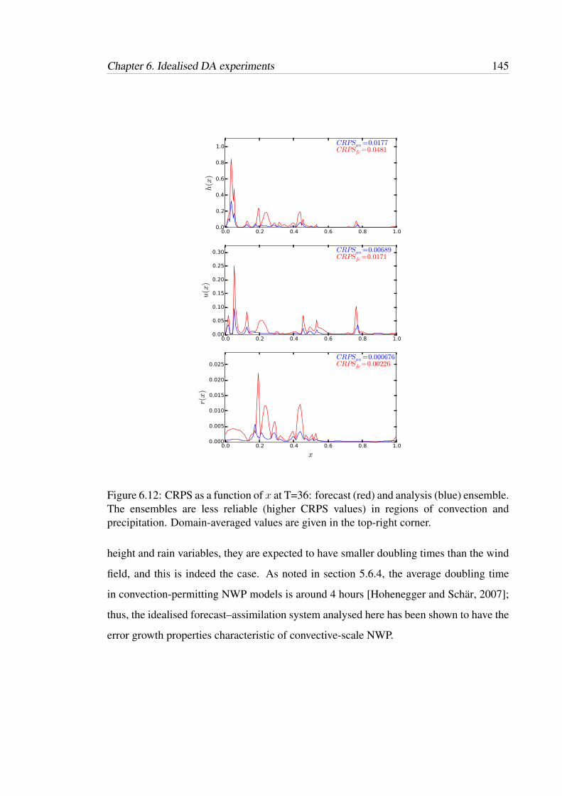
Chapter 6. Idealised DA experiments 145
0.0 0.2 0.4 0.6 0.8 1.00.0
0.2
0.4
0.6
0.8
1.0
h(x
)
CRPSan=0.0177CRPSfc=0.0481
0.0 0.2 0.4 0.6 0.8 1.00.00
0.05
0.10
0.15
0.20
0.25
0.30
u(x
)
CRPSan=0.00689CRPSfc=0.0171
0.0 0.2 0.4 0.6 0.8 1.0
x
0.000
0.005
0.010
0.015
0.020
0.025
r(x)
CRPSan=0.000676CRPSfc=0.00226
Figure 6.12: CRPS as a function of x at T=36: forecast (red) and analysis (blue) ensemble.The ensembles are less reliable (higher CRPS values) in regions of convection andprecipitation. Domain-averaged values are given in the top-right corner.
height and rain variables, they are expected to have smaller doubling times than the wind
field, and this is indeed the case. As noted in section 5.6.4, the average doubling time
in convection-permitting NWP models is around 4 hours [Hohenegger and Schar, 2007];
thus, the idealised forecast–assimilation system analysed here has been shown to have the
error growth properties characteristic of convective-scale NWP.

146 Chapter 6. Idealised DA experiments
5 10 15 20 250
50
100
150
200
250
300
Count
Mean=4.14Median=3
Total=640/640
5 10 15 20 250
50
100
150
200
Count
Mean=5.68Median=5
Total=636/640
5 10 15 20 25
Time (hrs)
0
50
100
150
200
250
300
350
Count
Mean=5.18Median=3
Total=635/640
Error-doubling time: histogram
Figure 6.13: Histograms of the error-doubling times (5.6.4) for 640 24-hour forecastsinitialised using analysis increments from the idealised forecast-assimilation system.From top to bottom: h, u, r. The average doubling time in convection-permitting NWPmodels is around 4 hours.

Chapter 6. Idealised DA experiments 147
6.3 Synopsis
The data assimilation techniques of chapter 5 have been applied to the modified shallow
water model described in the first part of this study, with the aim of further demonstrating
its suitability for investigating DA algorithms at convective scales. The exploratory
investigation presented in this chapter, together with the dynamical analysis in chapter
4, indicates that a well–tuned idealised forecast–assimilation system can be obtained that
exhibits some characteristics relevant for convective-scale NWP and possesses sufficient
error growth for meaningful hourly–cycled DA at the kilometre–scale.
Twin–model experiments have been established in the imperfect model scenario using
the stochastic EnKF assimilation algorithm. The nature run simulates varied dynamics,
with convection and precipitation occurring due to topographic forcing only, and is used
to generate pseudo-observations and as a verifying surrogate of the truth. The forecast
model runs on a coarser horizontal grid (akin to a 2.5km gridsize) and is only able to
resolve partially the convection and precipitation field, thus mimicking the state-of-the-
art of convection-permitting NWP models. An assimilation update frequency of one hour
is also analogous to high-resolution DA systems. A basic observing system is imposed in
which all variables are observed directly (hence the observation operatorH is linear) at a
given density ∆y.
Tuning a forecast–assimilation system is performed to optimise the filter configuration
to give the lowest analysis error. In an idealised setting, the observing system (in
this case density and error) should be tuned alongside the filter configuration to
produce an idealised system that demonstrates attributes of an operational system. The
process of tuning the idealised system and arriving at a well-tuned experiment with an
observational influence similar to that of NWP has been recounted here. Given the simple
observing system and strong nonlinearities of the forecast model, the EnKF performs
adequately when supplemented with techniques to combat undersampling. Indeed, as

148 Chapter 6. Idealised DA experiments
0 50 100 150 200x
0.0
0.2
0.4
0.6
0.8
1.0%
Lloc=50
Lloc=80
Lloc=200
Lloc=∞
h hu hr
h
hu
hr
ρ with Lloc=80
h hu hr
h
hu
hr
Cf
h hu hr
h
hu
hr
ρ Cf
1.0
0.8
0.6
0.4
0.2
0.0
0.2
0.4
0.6
0.8
1.0
Figure 6.14: Facets of localisation: taper functions, a localising matrix, and the effecton correlation matrices. Top left: Gaspari-Cohn taper functions %(x) for a given cut-offlength-scale Lloc. Top right: the 3×3 block localisation matrix ρ ∈ Rn×n computed from% with Lloc = 80. Bottom left: a correlation matrix after T=36 cycles from the experimentwith ∆y = 40, γm = 1.01, Lloc = ∞. Notice the strength of off-diagonal correlations.Bottom right: the same correlation matrix localised using the above ρ with Lloc = 80.This suggests that applying localisation in this setting suppresses true covariances, therebydegrading the analysis.

Chapter 6. Idealised DA experiments 149
demonstrated in section 6.2.1, additive inflation is crucial for maintaining satisfactory
filter performance. By comparing the ensemble spread and the RMS error of the ensemble
mean, it is shown that certain filter configurations yield ensembles that adequately
estimate the forecast errors. The overall skill of the ensembles is assessed using the CRPS
as well. Good performance is achieved with a reasonable (i.e., not too large) multiplicative
inflation factor of γm = 1.01. Hamill et al. [2001] find that inflation factors of only 1% or
2% are adequate with an ensemble size of 100 and a global isentropic two-layer model,
and Houtekamer and Zhang [2016] note that inflation values close to one are desirable.
For the idealised experiments presented here, localisation degrades the analysis. This is
somewhat at odds with operational practice in which some form of localisation is crucial
for ensemble-based DA systems to function satisfactorily. In the operational DA problem,
N p n (where N is O(10 − 100), p is O(107) and n is O(109)) exemplifies
severe rank-deficiency. The subspace spanned by the ensemble is extremely restrictive
and confines the observations to an insufficient number of directions, especially given the
indirect nature of the vast majority of observations. Localisation increases the effective
degrees of freedom of the system, thereby increasing the rank of the problem and making
the high-dimensional problem tractable.
On the other hand, the dimensions corresponding to the idealised system are p < N < n
where p = 15, 30,N = 40, and n = 600. This is clearly very different to an operational
setting; by their very definition, idealised systems are low order and do not seek to match
this aspect of operational systems. In particular, N > p and the observations are direct.
This suggests that there is no need for localisation in this specific experimental setting: the
observations lie within the spread of the ensembles (note the observations in figure 6.10)
and so there is no need to increase the rank of the problem. This issue is also encountered
by Anderson [2012, 2015] in an idealised setting with N > p. The fact the analysis is
increasingly degraded by stricter localisation (i.e., decreasing Lloc) suggests also that real
correlations are being suppressed in this case. Indeed, the correlation matrices plotted

150 Chapter 6. Idealised DA experiments
in figure 6.14 show that ‘signal’ rather than ‘noise’ is being removed by localisation.
However, it should be stressed that this is only one realisation of a possible observing
system: treating the observations differently (e.g., vary the error σσσ and/or observation
operatorH) may lead to a different conclusion concerning the role of localisation.
Finally, the analysis increments from a well-tuned experiment with ∆y = 40, γm =
1.01, Lloc =∞ were used to initialise staggered 24-hour forecasts as part of an idealised
ensemble prediction system. An analysis of the error-growth statistics exposes doubling
times comparable with convection-permitting NWP models.

151
Chapter 7
Conclusion
High–resolution ‘convection–permitting’ NWP models are now commonplace and
are able to resolve some of the finer–scale features associated with convection and
precipitation. However, increasing the spatial resolution is not a panacea; the so-called
‘grey-zone’ – the range of horizontal scales in which convective processes are being partly
resolved dynamically and partly by subgrid parametrisations – poses many challenges for
NWP, including how best to tackle the assimilation problem. This thesis concerns the
development of an idealised model of convective-scale Numerical Weather Prediction and
its use in inexpensive data assimilation experiments. A summary of the work undertaken
and research findings is given in section 7.1, before the aims presented in the introduction
are revisited in section 7.2. Finally, potential ideas for taking this work further are
suggested in section 7.3.
7.1 Summary
Idealised models are designed to represent some essential features of the physical
problem at hand and offer a computationally inexpensive tool for researching assimilation
algorithms. A great deal of preliminary analysis on the performance and suitability of

152 Chapter 7. Conclusion
potential DA algorithms is conducted using the low-order models of Lorenz [Lorenz,
1986, 1996; Lorenz and Emanuel, 1998; Lorenz, 2005]. However, there is a vast gap
between the complexity of these models and operational NWP models which integrate
the primitive equations of motion [Kalnay, 2003].
The first part of this thesis, ‘Dynamics’, develops and analyses an idealised fluid
dynamical model of intermediate complexity (extending that of Wursch and Craig [2014];
WC14) that attempts to fill this gap in hierarchy of complexity of ‘toy’ models. It modifies
the shallow water equations (SWEs) to model some dynamics of cumulus convection and
associated precipitation effects. A full description and the physical basis of the model
is given in chapter 2. Changes to the dynamics are brought about by the exceedance
of two threshold heights Hc and Hr, akin to (i) the level of free convection, and (ii)
the onset of precipitation. When the fluid exceeds these heights, the classical shallow
water dynamics are altered to include a representation of conditional instability (leading
to a convective updraft) and idealised moisture transport with associated downdraft and
precipitation effects. The main differences compared to the model proposed in WC14
are the inclusion of rotation and corresponding transverse flow and, more significantly,
the removal of various diffusive terms in the governing equations included for numerical
stability. The numerical model of WC14 is very sensitive to the diffusive terms and not
very robust to changes, making it difficult to explore different experimental set-ups.
Despite the non-trivial modifications to the parent equations, it is shown mathematically
that the model remains hyperbolic and can be integrated accordingly using a
discontinuous Galerkin (DG) finite element framework that deals robustly with systems
of partial differential equations with non-conservative products (NCPs; Rhebergen et al.
[2008]). However, hitherto unknown issues with topography and well-balancedness in
DG0 discretisations necessitated a novel approach to the problem. To this end, a stable
solver has been developed in chapter 3 that combines the method of Rhebergen et al.
[2008] for treating the NCPs and the method of Audusse et al. [2004] which ensures a

Chapter 7. Conclusion 153
well-balanced scheme that preserves non-negativity.
To test the solver and investigate the distinctive dynamics of the modified model, a series
of simulations are conducted in chapter 4 and the resulting solutions examined with
reference to the classical shallow water theory. Two scenarios are explored, based on
(i) the Rossby adjustment problem, and (ii) non-rotating flow over topography; within
these scenarios, a hierarchy of model ‘cases’ is employed to illustrate the effect that
exceeding the threshold heights Hc < Hr has on the dynamics. Crucially, the model
reduces exactly to the standard SWEs in non-convecting, non-precipitating regions; this
is clear analytically and the experiments confirm that the correct shallow water dynamics
are retained in the numerics.
The shift from large- to convective-scale NWP is in some sense a shift from balanced to
unbalanced dynamics. Traditional DA systems developed for large-scale NWP exploit
the fact the midlatitude dynamics at the synoptic scale are close to geostrophic and
hydrostatic balance. However, this balance is no longer manifest at smaller scales where
rotation no longer dominates and vertical accelerations modulate the flow. The modified
model exhibits important aspects of convective-scale dynamics relating to the disruption
of these large-scale balance principles. The Rossby adjustment scenario illustrates the
breakdown of geostrophic balance in the presence of convection and precipitation and
hydrostatic balance is disrupted implicitly by the modified pressure when the level of
free convection Hc is exceeded. The simulations show that the model is able to capture
features relating to convection and orographic forcing, such as the initiation of so-called
‘daughter’ convection cells away from the parent cell by gravity wave propagation, and
convection downstream from a ridge. There are well-known non-trivial steady state
solutions for flow over a parabolic ridge in the classical shallow water theory. The
model satisfies these and a novel extended set of solutions derived for the ‘convection’
and ‘rain’ case. Given the physical description and numerical investigation presented
here, the modified shallow water model is able to simulate some fundamental dynamical

154 Chapter 7. Conclusion
processes associated with convecting and precipitating weather systems, thus suggesting
that it is a suitable candidate for investigating DA algorithms at convective scales.
It is widely accepted that ensemble-based DA algorithms offer most success at convective
scales. These methods use an ensemble of forecast states to approximate the forecast
error covariances. These flow-dependent error statistics are able to capture nonlinear
and intermittent aspects of the convective-scale flow that a static covariance matrix
method would not. The stochastic ensemble Kalman filter (EnKF), in combination with
techniques to tackle undersampling, offers a robust algorithm with which to investigate the
suitability of the model in idealised forecast-assimilation experiments. The classical DA
problem is outlined in chapter 5 alongside the theoretical and practical aspects of Kalman
filtering. Experiments are carried out in the twin-model setting and, where possible,
mimic characteristics of NWP. The forecast model is designed to partially resolve the
convection and precipitation fields while observations are sampled from a nature run
integrated at a higher resolution. Given this mismatch between the forecast and “truth”,
it is shown that additive inflation is crucial for maintaining satisfactory filter performance
and preventing filter divergence, and that there is sufficient error growth for meaningful
hourly-cycled DA at the kilometre–scale.
The observing system and filter configuration can be tuned to yield a forecast-assimilation
system that satisfactorily estimates the forecast errors and has an average observational
influence similar to that of operational NWP. Reasonable multiplicative inflation factors
are obtained, but the dimensions of the problem, namely that the size of the ensemble is
larger than the number of observations, mean that there is no need for localisation. This
is somewhat unfortunate as localisation is a crucial aspect of operational ensemble-based
DA systems. It would therefore be desirable to have a situation that requires localisation
in the idealised setting. Ideas for how this can be achieved, along with other suggestions
for future work, are discussed in section 7.3.
Nonetheless, the results of the idealised DA experiments and tuning process described

Chapter 7. Conclusion 155
in chapter 6, along with the dynamics investigation, indicate that the idealised fluid
model is a suitable tool for controlled forecast–assimilation experiments in the presence
of convection and precipitation.
7.2 Aims revisited
In the introductory chapter, a set of aims was proposed to direct the research carried out
in this thesis; these are revisited briefly here.
1. Establish a physically plausible idealised fluid dynamical model with
characteristics of convective–scale NWP.
(a) Present a physical and mathematical description of the model, based on the
rotating shallow water equations and extending the model of WC14.
Starting from the rotating SWEs, the modifications are introduced and the
physical reasoning behind them is discussed in detail in chapter 2, with
reference to the dynamics of cumulus convection. Despite the modifications,
and unlike the model of WC14, the model is shown to be hyperbolic.
(b) Derive a stable and robust numerical solver based on the discontinuous
Galerkin finite element method.
In chapter 3, the so-called ’non-conservative product’ (NCP) flux is derived
which captures the nonlinear switches of the threshold heights. Since the goal
is to use the model in inexpensive DA experiments, computational efficiency
is paramount, implying a zero-order DG discretisation. However, hitherto
unknown issues concerning topography and well-balancedness at this order
necessitated an innovative approach that merged the NCP theory and the
method of Audusse et al. [2004]. Stability is ensured via a dynamic time

156 Chapter 7. Conclusion
step that is robust to changes in the dynamics and maintains non-negativity of
h.
(c) Investigate the distinctive dynamics of the model with comparison to the
classical shallow water theory.
A thorough investigation of the model’s dynamics is conducted numerically
in chapter 4. A hierarchy of model cases illustrates the effect of convection
(exceeding Hc) and precipitation (exceeding Hr) with reference to the
classical shallow water dynamics in two scenarios: (i) Rossby adjustment
problem and (ii) flow over topography.
2. Show that the model provides an interesting test bed for investigating DA algorithms
in the presence of complex dynamics associated with convection and precipitation.
(a) Demonstrate a well–tuned forecast–assimilation system using the ensemble
Kalman filter assimilation algorithm.
The results of idealised forecast–assimilation experiments and the tuning
process are presented in chapter 6. By permuting through observational
density, inflation factors, and localisation length-scales, a well–tuned
observing system and filter configuration is achieved that adequately estimates
the forecast error and has an average observational influence similar to NWP.
(b) Elucidate its relevance for convective–scale NWP and DA.
The forecast–assimilation system has been designed to mimic aspects of
convective-scale NWP and DA. The forecast model has a grid size of∼ 2.5km
and only partially resolves the convection and precipitation fields, while
observations are sampled from a higher resolved nature run. The hourly
update frequency is comparable to operational high-resolution NWP and
error-doubling time statistics reflect those of convection-permitting models
in a cycled forecast–assimilation system. Ideally, realising an experiment that
requires localisation would be more relevant as this is a crucial aspect of an

Chapter 7. Conclusion 157
operational system. Suggestions for how this might be achieved follow.
7.3 Future work: plans and ideas
This thesis has developed an idealised model for research purposes that offers a wealth
of opportunities for further research in numerous directions. The model of WC14
has deservedly received a great deal of attention for its fluid dynamical approach to
convective-scale DA research but suffers from a lack of robustness that prevents rigorous
use. It is hoped that the mathematically cleaner formulation and stable solver arising
from this research provides a useful tool to the community and facilitates other studies in
the field of convective-scale DA research. To this end, we plan to integrate the model’s
source code into EMPIRE (Employing MPI for Researching Ensembles), an open-source
repository for interfacing numerical models with DA methods [Browne and Wilson,
2015], and a journal article is in preparation that covers the model and its dynamics
(chapters 2–4).
The idealised experiments presented in chapter 6 should be considered a preliminary
investigation that demonstrate the model’s suitability for this purpose. There remains
plenty of scope for further work, with myriad experimental set–ups to explore and
concepts to investigate. To conclude the thesis, a few comments and suggestions for
extensions to this work are proposed.
1. Comments on additive inflation and the QQQ matrix
In the EnKF algorithm implemented in this thesis, additive inflation is applied to the
forecast states xfj right before the assimilation step, while multiplicative inflation
follows the assimilation step and is applied to the analysis states xaj . However,
additive inflation is usually applied incrementally per time step throughout the
forecast stage, or alternatively after the assimilation step (and ideally after the

158 Chapter 7. Conclusion
multiplicative inflation is applied). Adding Gaussian noise immediately prior to
the assimilation has the potential to dominate any non-Gaussianity resulting from
the nonlinear forecast model. While this is beneficial to the EnKF algorithm,
which assumes Gaussian statistics, it does not give the forecast model a chance
to evolve the Gaussian additive error into something non-Gaussian, which is more
like operational NWP.
Operational NWP does not have access to a “truth” forecast, like the nature run xt
in idealised experiments. As such, an idealised configuration seeking to mimic
an operational system should not incorporate the nature run in the assimilation
algorithm itself. Here, as explained in section 6.2.1, the QQQ matrix is updated each
cycle using the nature run, which is not a realistic feature. Ideally, QQQ should be
computed independently of the cycled forecast/assimilation system and having no
dependence on the observing system, so that the same matrix is used throughout
the experiments. EstimatingQQQ is in itself a considerable area of research that could
benefit from studies using intermediate-complexity models such as this one.
2. Conduct experiments with rotation
The idealised forecast–assimilation experiments conducted in this thesis consider
non-rotating flow over topography. As demonstrated in chapter 4, the modified
model is able to simulate interesting dynamics with Coriolis rotation effects and
transverse velocity v. An obvious next step is to conduct idealised DA experiments
in the presence of rotating convection and precipitation. This is achievable with
zero bottom topography but, in its current form, the numerical solver cannot
accommodate rotating flow over topography. However, this should be further
developed.
3. Change the way the system is observed
The observing system, embodied in the observation operator H, has a critical
impact on the behaviour and performance of a forecast–assimilation system. The

Chapter 7. Conclusion 159
experiments of chapter 6 employ a basic observing system in which all variables
are observed directly and homogeneously in space (so thatH is linear).
(a) Before considering a nonlinear H, it would be interesting to see the effect
of observing a subset of the variables only, e.g., only observing h. The role
of the forecast error covariance matrix Pf is to partition the observational
information throughout the state space using the estimated spatial correlations
between variables. By only observing, say, h, the ability of Pf to do this
can be ascertained. This could also necessitate localisation as the role of the
Pf and effect of spurious correlations increases. Another way to increase the
need for localisation is to use a larger domain, thereby increasing the distance
from some observations and subsequently decreasing true correlations at these
distances. Spurious correlations will then be more noticeable.
(b) Operational observing systems are heterogeneous and nonlinear. A nonlinear
observing system can be introduced to the idealised system by, e.g., observing
wind speed and direction (in the rotating case) or simply an arbitrary nonlinear
function of the variables, e.g.,√h. A nonlinearH, coupled with the nonlinear
dynamics of convection and precipitation in the forecast modelM, would be
expected to push the limits of linear assimilation algorithms such as the EnKF.
(c) The advent of satellites in the 1970s offered a new extensive source of
observations and brought huge benefit to NWP. Nowadays, many of the
observations come from satellites (or other remote sensing techniques such
as radar) and these are expected to play a critical role in advancing high-
resolution DA. However, they pose huge challenges and the question of how
best to assimilate such a vast quantity of indirect observations is a major topic
of research. It would be possible to mimic satellite observing systems in an
idealised setting by having periodic observations localised in space and time
and a simplified radiative transfer model. The model with such an observing
160 Chapter 7. Conclusion
system would provide an interesting testbed for satellite DA research.
4. Comparison of algorithms
Idealised models are most typically employed in a framework to compare the
performance of different assimilation algorithms (e.g., Fairbairn et al. [2014]).
The model could be used to compare methods in the presence of convection and
precipitation. For example, how does the EnKF perform against a hybrid ensemble–
variational method or a fully nonlinear filter? The debate around nonlinear data
assimilation (section 5.4.3) is growing with the resolution of NWP models; an
idealised model with highly nonlinear convective processes is a useful tool for
furthering research in this direction.

161
Appendices
A The model of Wursch and Craig [2014]
The augmented shallow water system employed by Wursch and Craig [2014] provides
a computationally inexpensive yet physically plausible environment for convective-scale
data assimilation research. It extends the shallow water equations (SWEs) to include the
transport of moisture by introducing a (dimensionless) ‘water mass fraction’ r which is
coupled to the momentum equation by modifying the geopotential Φ. The system reads:
∂th+ ∂x(hu) = Kh∂xxh, (A.1a)
∂tu+ u∂xu+ ∂x(Φ + γr) = Ku∂xxu, (A.1b)
∂tr + u∂xr = Kr∂xxr − αr −
β∂xu, if Z > Hr and ∂xu < 0;
0, otherwise,(A.1c)
where
Φ =
Φc + gH, for Z > Hc;
gZ, otherwise,(A.2)
Here Z = h + b is the absolute fluid layer height, b = b(x) is the topography and
h = h(x, t) is the free-surface height. The geopotential Φ is modified when total height
exceeds a threshold Hc, above which it takes a (low) constant value Φc. Model ‘rain’ is
produced when the total height exceeds a higher ‘rain’ thresholdHr in addition to positive

162 Appendices
wind convergence (∂xu < 0). Elsewhere, α and β are positive constants controlling the
removal and production of rain, respectively, and γ is a scaling constant with geopotential
units, m2s−2. The diffusion coefficients Kh, Ku, and Kr are tuned to stabilise the model
for a specific numerical implementation and are the dominant controlling factor of the
subsequent solutions.

Appendices 163
B Non-negativity preserving numerics
Schemes that preserve the non-negativity of h are able to efficiently compute the ‘dry’
states where h = 0 (e.g., Audusse et al. [2004]; Bokhove [2005]; Xing et al. [2010]) by
reconstructing the computational variables and modifying the numerical flux function via
a positivity-preserving limiter. Given a derived time-step criterion, this yields a stable,
well-balanced scheme that preserves steady states, non-negativity and conservation of h.
The following appendix presents the scheme of Audusse et al. [2004], a detailed proof
of the non-negativity preservation including the derived elemental time step, and a test
simulation that requires the computation of dry states and moving wet/dry boundaries.
Scheme of Audusse et al. [2004]
The spatial domain x ∈ [0, L] is discretised into cells Kk = [xk−1/2, xk+1/2] for k =
1, 2, ..., N with N + 1 nodes 0 = x1/2, x3/2, ..., xN−1/2, xN+1/2 = L. Cell lengths |Kk| =
xk+1/2 − xk−1/2 may vary. The computational variables Uk(t) in finite volume methods
approximate the model states U(x, t) as a piecewise constant function in space (i.e., as a
cell average):
Uk(t) =1
|Kk|
∫Kk
U(x, t)dx. (B.3)
Integrating the system (2.1) over the cell Kk and using (B.3) yields the space-discretised
scheme:d
dtUk +
1
|Kk|[Fk+1/2 −Fk−1/2
]+ S(Uk) = 0, (B.4)
where Fk+1/2 = F(UL,UR) = F(U(xk+1/2, t)) is the flux evaluated at the node xk+1/2
using the computational states to the left and right of the node.
The first-order finite volume scheme for the h-equation using a forward Euler time

164 Appendices
discretisation is:
hn+1k = hnk − µ
[Fh(U−k+1/2,U
+k+1/2)−F
h(U−k−1/2,U+k−1/2)
](B.5)
where µ = 4t/|Kk|, F is a numerical flux, and U±k+1/2 are reconstructed states to the left
and right of node xk+1/2:
U−k+1/2 =
h−k+1/2
h−k+1/2uk
, U+k+1/2 =
h+k+1/2
h+k+1/2uk+1
, (B.6)
with:
h−k+1/2 = max (0, hk + bk −max(bk, bk+1)) , (B.7a)
h+k+1/2 = max (0, hk+1 + bk+1 −max(bk, bk+1)) . (B.7b)
For the numerical flux F through node xk+1/2, take the HLL flux (after Harten et al.
[1983]):
Fh(U−k+1/2,U+k+1/2) =
h−k+1/2uk, if SLk+1/2 > 0;
FHLLk+1/2, if SLk+1/2 < 0 < SRk+1/2;
h+k+1/2uk+1, if SRk+1/2 < 0;
(B.8)
where:
FHLLk+1/2 =h−k+1/2ukS
Rk+1/2 − h
+k+1/2uk+1S
Lk+1/2 + SLk+1/2S
Rk+1/2(h
+k+1/2 − h
−k+1/2)
SRk+1/2 − SLk+1/2
,
(B.9)

Appendices 165
and the numerical speeds are given by:
SLk+1/2 = min(uk −
√gh−k+1/2 , uk+1 −
√gh+k+1/2
), (B.10a)
SRk+1/2 = max(uk +
√gh−k+1/2 , uk+1 +
√gh+k+1/2
). (B.10b)
Note that, by construction of (B.7), the following inequalities hold:
0 ≤ h−k+1/2 ≤ hk, 0 ≤ h+k+1/2 ≤ hk+1. (B.11)
Theorem
For the scheme described above in (B.5) to (B.10), if hnk , hnk±1 ≥ 0, then hn+1k ≥ 0 (given
a time-step criterion, to be derived).
Proof
There are 9 different cases that the discretised h-equation (B.5) can take, each
corresponding to the correct flux term for the given numerical speed. For each case, it
is shown that if hnk , hnk±1 ≥ 0, then hn+1k ≥ 0 for a given a time-step criterion. Finally,
these criteria are amalgamated into a single elemental time step restriction covering all 9
cases.
Case 1: if (SLk+1/2 > 0) ∧ (SLk−1/2 > 0), then:
hn+1k = hnk − µ
[h−k+1/2uk − h
−k−1/2uk−1
]=
[1− µuk
h−k+1/2
hnk
]hnk +
[µuk−1
h−k−1/2hnk−1
]hnk−1.
The expression in the second bracket is always non-negative since uk−1 > 0 and (B.11).

166 Appendices
The first bracket is non-negative given the time-step restriction:
µukh−k+1/2
hnk≤ 1. (B.12)
Given this criterion, we see that hn+1k is a linear combination of hnk , hnk±1 and all the
coefficients are non-negative. Thus, hn+1k ≥ 0.
Case 2: if (SRk+1/2 < 0) ∧ (SRk−1/2 < 0), then:
hn+1k = hnk − µ
[h+k+1/2uk+1 − h+k−1/2uk
]=
[1 + µuk
h+k−1/2hnk
]hnk +
[−µuk+1
h+k+1/2
hnk+1
]hnk+1.
The expression in the second bracket is always non-negative since uk+1 < 0 and (B.11).
Since uk < 0, the first bracket is non-negative given the time-step restriction:
− µukh+k−1/2hnk
≤ 1. (B.13)
Thus, hn+1k ≥ 0.
Case 3: if (SRk+1/2 < 0) ∧ (SLk−1/2 > 0), then:
hn+1k = hnk − µ
[h+k+1/2uk+1 − h−k−1/2uk−1
]= hnk +
[−µuk+1
h+k+1/2
hnk+1
]hnk+1 +
[µuk−1
h−k−1/2hnk−1
]hnk−1.
Since uk+1 < 0, uk−1 > 0, and (B.11), all the coefficients are non-negative. Thus,
hn+1k ≥ 0.

Appendices 167
Case 4: if (SLk+1/2 > 0) ∧ (SRk−1/2 < 0), then:
hn+1k = hnk − µ
[h−k+1/2uk − h
+k−1/2uk
]=
[1− µuk
h−k+1/2 − h+k−1/2
hnk
]hnk .
But SLk+1/2 > 0 =⇒ uk > 0 while SRk−1/2 < 0 =⇒ uk < 0, which is clearly a
contradiction. Thus, the case (SLk+1/2 > 0) ∧ (SRk−1/2 < 0) is not possible.
Case 5: if (SLk+1/2 < 0 < SRk+1/2) ∧ (SLk−1/2 < 0 < SRk−1/2), then:
hn+1k = hnk − µ
[FHLLk+1/2 −FHLLk−1/2
]= hnk − µ
[h−k+1/2ukS
Rk+1/2 − h
+k+1/2uk+1S
Lk+1/2 + SLk+1/2S
Rk+1/2(h
+k+1/2 − h
−k+1/2)
SRk+1/2 − SLk+1/2
]
+ µ
[h−k−1/2uk−1S
Rk−1/2 − h
+k−1/2ukS
Lk−1/2 + SLk−1/2S
Rk−1/2(h
+k−1/2 − h
−k−1/2)
SRk−1/2 − SLk−1/2
]
=
[1− µ
SRk+1/2
4Sk+1/2
h−k+1/2
hnk
(uk − SLk+1/2
)− µ
SLk−1/24Sk−1/2
h+k−1/2hnk
(uk − SRk−1/2
)]hnk
+
[µSLk+1/2
4Sk+1/2
h+k+1/2
hnk+1
(uk+1 − SRk+1/2
)]hnk+1
+
[µSRk−1/24Sk−1/2
h−k−1/2hnk−1
(uk−1 − SLk−1/2
)]hnk−1,
where 4Sk+1/2 = SRk+1/2 − SLk+1/2 > 0. Clearly the sign of the coefficients depends on
the sign of the twice-underlined terms, defined shorthand as:
SL,uk+1/2 := uk − SLk+1/2, SR,uk+1/2 := uk+1 − SRk+1/2. (B.14)

168 Appendices
Then the scheme reads:
hn+1k =
[1− µ
SRk+1/2SL,uk+1/2
4Sk+1/2
h−k+1/2
hnk− µ
SLk−1/2SR,uk−1/2
4Sk−1/2
h+k−1/2hnk
]hnk
+
[µSLk+1/2S
R,uk+1/2
4Sk+1/2
h+k+1/2
hnk+1
]hnk+1 +
[µSRk−1/2S
L,uk−1/2
4Sk−1/2
h−k−1/2hnk−1
]hnk−1.
Examining the conditions of the numerical speeds, it can be concluded that:
(SLk+1/2 < 0 < SRk+1/2
)=⇒
(SL,uk+1/2 > 0
)∧(SR,uk+1/2 < 0
). (B.15)
Therefore, since SLk+1/2 < 0 and noting (B.11), the coefficient of hnk+1 is always
non-negative. Similarly, since SRk−1/2 > 0, the coefficient of hnk−1 is always non-
negative. Demanding the coefficent of hnk to be non-negative yields the following time-
step restriction:
µ
[SRk+1/2S
L,uk+1/2
4Sk+1/2
h−k+1/2
hnk+SLk−1/2S
R,uk−1/2
4Sk−1/2
h+k−1/2hnk
]≤ 1. (B.16)
Due to (B.15), the expression in square brackets is always non-negative. Thus, given this
time-step restriction, hn+1k ≥ 0.

Appendices 169
Case 6: if (SLk+1/2 < 0 < SRk+1/2) ∧ (SLk−1/2 > 0), then:
hn+1k = hnk − µ
[FHLLk+1/2 − h−k−1/2uk−1
]= hnk − µ
[h−k+1/2ukS
Rk+1/2 − h
+k+1/2uk+1S
Lk+1/2 + SLk+1/2S
Rk+1/2(h
+k+1/2 − h
−k+1/2)
SRk+1/2 − SLk+1/2
− h−k−1/2uk−1]
=
[1− µ
SRk+1/2SL,uk+1/2
4Sk+1/2
h−k+1/2
hnk
]hnk +
[µSLk+1/2S
R,uk+1/2
4Sk+1/2
h+k+1/2
hnk+1
]hnk+1
+
[µuk−1
h−k−1/2hnk−1
]hnk−1,
where 4Sk+1/2 = SRk+1/2 − SLk+1/2 > 0. Noting (B.11), (B.15), and the numerical
speed conditions (uk−1 > 0), it is clear that the coefficients of hnk±1 are always non-
negative. Demanding the coefficent of hnk to be non-negative yields the following time-
step restriction:
µ
[SRk+1/2S
L,uk+1/2
4Sk+1/2
h−k+1/2
hnk
]≤ 1. (B.17)
Due to (B.15), the expression in square brackets is always non-negative. Thus, given this
time-step restriction, hn+1k ≥ 0.
Case 7: if (SLk+1/2 < 0 < SRk+1/2) ∧ (SRk−1/2 < 0), then:
hn+1k = hnk − µ
[FHLLk+1/2 − h+k−1/2uk
]= hnk − µ
[h−k+1/2ukS
Rk+1/2 − h
+k+1/2uk+1S
Lk+1/2 + SLk+1/2S
Rk+1/2(h
+k+1/2 − h
−k+1/2)
SRk+1/2 − SLk+1/2
− h+k−1/2uk]
=
[1− µ
SRk+1/2SL,uk+1/2
4Sk+1/2
h−k+1/2
hnk+ µuk
h+k−1/2hnk
]hnk +
[µSLk+1/2S
R,uk+1/2
4Sk+1/2
h+k+1/2
hnk+1
]hnk+1,
where 4Sk+1/2 = SRk+1/2 − SLk+1/2 > 0. Noting (B.11), (B.15), it is clear that the

170 Appendices
coefficient of hnk+1 is always non-negative. Demanding the coefficent of hnk to be non-
negative yields the following time-step restriction:
µ
[SRk+1/2S
L,uk+1/2
4Sk+1/2
h−k+1/2
hnk− uk
h+k−1/2hnk
]≤ 1. (B.18)
Due to (B.15) and the numerical speed condition (uk < 0), the expression in square
brackets is always non-negative. Thus, given this time-step restriction, hn+1k ≥ 0.
Case 8: if (SLk+1/2 > 0) ∧ (SLk−1/2 < 0 < SRk−1/2), then:
hn+1k = hnk − µ
[h−k+1/2uk −F
HLLk−1/2
]= hnk − µ
[h−k+1/2uk
−h−k−1/2uk−1S
Rk−1/2 − h
+k−1/2ukS
Lk−1/2 + SLk−1/2S
Rk−1/2(h
+k−1/2 − h
−k−1/2)
SRk−1/2 − SLk−1/2
]
=
[1− µuk
h−k+1/2
hnk− µ
SLk−1/2SR,uk−1/2
4Sk−1/2
h+k−1/2hnk
]hnk +
[µSRk−1/2S
L,uk−1/2
4Sk−1/2
h−k−1/2hnk−1
]hnk−1,
where 4Sk−1/2 = SRk−1/2 − SLk−1/2 > 0. Noting (B.11), (B.15), it is clear that the
coefficient of hnk−1 is always non-negative. Demanding the coefficent of hnk to be non-
negative yields the following time-step restriction:
µ
[ukh−k+1/2
hnk+SLk−1/2S
R,uk−1/2
4Sk−1/2
h+k−1/2hnk
]≤ 1. (B.19)
Due to (B.15) and the numerical speed condition (uk > 0), the expression in square
brackets is always non-negative. Thus, given this time-step restriction, hn+1k ≥ 0.

Appendices 171
Case 9: if (SRk+1/2 < 0) ∧ (SLk−1/2 < 0 < SRk−1/2), then:
hn+1k = hnk − µ
[h+k+1/2uk+1 −FHLLk−1/2
]= hnk − µ
[h+k+1/2uk+1
−h−k−1/2uk−1S
Rk−1/2 − h
+k−1/2ukS
Lk−1/2 + SLk−1/2S
Rk−1/2(h
+k−1/2 − h
−k−1/2)
SRk−1/2 − SLk−1/2
]
=
[1− µ
SLk−1/2SR,uk−1/2
4Sk−1/2
h+k−1/2hnk
]hnk +
[−µuk+1
h+k+1/2
hnk+1
]hnk+1
+
[µSRk−1/2S
L,uk−1/2
4Sk−1/2
h−k−1/2hnk−1
]hnk−1,
where 4Sk−1/2 = SRk−1/2 − SLk−1/2 > 0. Noting (B.11), (B.15), and the numerical
speed condition (uk+1 < 0), it is clear that the coefficient of hnk±1 is always non-
negative. Demanding the coefficent of hnk to be non-negative yields the following time-
step restriction:
µ
[SLk−1/2S
R,uk−1/2
4Sk−1/2
h+k−1/2hnk
]≤ 1. (B.20)
Due to (B.15), the expression in square brackets is always non-negative. Thus, given this
time-step restriction, hn+1k ≥ 0.
Elemental time step: for each case of numerical flux, it has been shown that hn+1k ≥ 0 for
hnk , hnk±1 ≥ 0 and a corresponding elemental time step restriction. We can combine these
cases into a concise expression for the elemental time-step4tk:
4tk =hnk |Kk|maxkDk
, (B.21)

172 Appendices
where the denominator Dk is given by:
Dk = ukh−k+1/2Θ(SLk+1/2) +
[SRk+1/2S
L,uk+1/2
4Sk+1/2
h−k+1/2
]Θ(−SLk+1/2)Θ(SRk+1/2)
− ukh+k−1/2Θ(−SRk−1/2) +
[SLk−1/2S
R,uk−1/2
4Sk−1/2h+k−1/2
]Θ(−SLk−1/2)Θ(SRk−1/2),
(B.22)
and Θ is the Heaviside function:
Θ(x) =
1, for x > 0,
0, for x ≤ 0.
(B.23)
The fluid depth thus remains non-negative provided the time step is less than the minimum
value of the elemental time step: 4t < 4tk.
Test case: parabolic bowl
A standard experiment for testing non-negativity preserving numerics in shallow water
flows is a sloped fluid height in parabolic bottom topography (see, e.g., Bokhove [2005];
Xing et al. [2010]). Physically, the problem models an oscillating lake in a basin, and
requires the computation of dry states and moving wet/dry boundaries. The parabolic
bottom topography is:
b(x) = h0
(xa
)2(B.24)
and the analytical fluid height is given by:
h(x, t) + b(x) = h0 −B2
4gcos(ωt)− B2
4g− Bx
2a
√8h0g
cos(ωt), (B.25)

Appendices 173
−5000 0 50000
5
10
15
20
t=400
x
h(x
,t)
−5000 0 50000
5
10
15
20
t=800
x
h(x
,t)
−5000 0 50000
5
10
15
20
t=1200
x
h(x
,t)
−5000 0 50000
5
10
15
20
t=1600
x
h(x
,t)
Figure B.1: Parabolic bowl problem at times t = 400, 800, 1200, 1600: blue - bottomtopography b, green - exact solution h + b , red - numerical solution h + b. Thecomputational domain is [−5000, 5000] with 1000 uniform cells.
where ω =√
2gh0/a . The fixed parameter values used here follow Xing et al. [2010]:
a = 3000, B = 5, h0 = 10. Figure B.1 shows the good agreement between numerical and
exact solutions at different times.

174 Appendices
C Well-balancedness: DG1 proof
For DG1 expansions (and higher), we can project the DG expansion coefficents of b such
that bh remains continuous across elements, then bR = bL and d(bk)/dt = 0. Then
all aspects of rest flow in (3.26) are satsified numerically and the scheme is truly well-
balanced. This is proved in this appendix for the space-DG1 discretisation. For reference,
the shallow water system (3.26) is characterised by:
UUU =
h
hu
b
, FFF (UUU) =
hu
hu2 + 12gh2
0
, GGG(UUU) =
0 0 0
0 0 gh
0 0 0
. (C.26)
The DG1 discretisation uses piecewise linear basis functions (i.e., first-order polynomials)
to approximate the trial function U and test function w and thereby discretise the weak
formulation (3.20) in space. The DG1 expansions are:
U ≈ Uh = U + ξU ; w ≈ wh = w + ξw. (C.27)
with mean and slope coefficients U = Uk(t) and U = Uk(t), where ξ ∈ (−1, 1) is a local
coordinate in the reference element Kk such that:
x = x(ξ) =1
2
(xk + xk+1 + |Kk|ξ
). (C.28)

Appendices 175
Thus, when ξ = −1, x = xk and ξ = 1, x = xk+1. Also note that dx = 12|Kk|dξ. We
evaluate the integrals in (3.20) with wi = wi|Kk and Ui = Ui|Kk as follows:
∫Kk
wi∂tUidx =
∫Kk
(wi + ξwi)∂t(U i + ξUi)dx
=1
2|Kk|
∫ 1
−1wi∂tU i + (wi∂tU i + wi∂tUi)ξ + (wi∂tUi)ξ
2dξ
=1
2|Kk|
[2wi∂tU i +
2
3wi∂tUi
]= |Kk|wi∂tU i +
1
3|Kk|wi∂tUi, (C.29)
∫Kk
−Fi∂xwidx = −∫Kk
Fi(U + ξU)∂x(wi + ξwi)dx
= −∫ 1
−1Fi(U + ξU)
2
|Kk|∂ξ(wi + ξwi)
1
2|Kk|dξ
= −wi∫ 1
−1Fi(U + ξU)dξ, (C.30)
∫Kk
wiGij∂xUjdx =
∫Kk
(wi + ξwi)Gij(U + ξU)∂x(U j + ξUj)dx
=
∫ 1
−1(wi + ξwi)Gij(U + ξU)
2
|Kk|∂ξ(U j + ξUj)
1
2|Kk|dξ
=
∫ 1
−1(wi + ξwi)Gij(U + ξU)Ujdξ
= wi
∫ 1
−1Gij(U + ξU)Ujdξ + wi
∫ 1
−1ξGij(U + ξU)Ujdξ. (C.31)
The flux terms in (3.20) are:
wi(x−k+1)P
pi (x−k+1, x
+k+1) = (wi + wi)|KkP
pi
((U i + Ui)|Kk , (U i − Ui)|Kk+1
), (C.32)
wi(x+k )Pmi (x−k , x
+k ) = (wi − wi)|KkPmi
((U i + Ui)|Kk−1
, (U i − Ui)|Kk). (C.33)

176 Appendices
The space-discretised scheme for means U i and slopes Ui is obtained by considering
coefficients of the test function means wi and slopes wi and taking wi = wi = 1
alternately for each element (again due to arbitrariness of wh):
0 = |Kk|∂tU i + Ppi(UL|Kk , UR|Kk+1
)− Pmi
(UL|Kk−1
, UR|Kk)
+
∫ 1
−1Gij(U + ξU)Ujdξ (C.34a)
0 =1
3|Kk|∂tUi + Ppi
(UL|Kk , UR|Kk+1
)+ Pmi
(UL|Kk−1
, UR|Kk)
−∫ 1
−1Fi(U + ξU)dξ +
∫ 1
−1ξGij(U + ξU)Ujdξ, (C.34b)
where UL = U+ U and UR = U− U are the trace values to the left and right of a element
edge.
Here it is shown analytically that when taking a linear path and using first-order expansion
for the model states and test functions, rest flow in the shallow water system (C.26)
remains at rest and the non-constant topography b does not evolve as long as bh remains
continuous across elements. The semi-discrete scheme is given by (C.34) and we evaluate
the integrals therein for rest flow, and check the following:
d
dt(hk + bk) = 0,
d
dt(hk + bk) = 0,
d
dt(huk) = 0,
d
dt(huk) = 0. (C.35)
For i = 1, 3, integrals involving G are zero. For i = 2:
∫ 1
−1G2j(U + ξU)Ujdξ = g
∫ 1
−1(h+ ξh)bdξ = g
∫ 1
−1(hb+ hbξ)dξ = 2ghb, (C.36)∫ 1
−1ξG2j(U + ξU)Ujdξ = g
∫ 1
−1ξ(h+ ξh)bdξ = g
∫ 1
−1(hbξ + hbξ2)dξ =
2
3ghb.
(C.37)
with the first integral featuring in the equation for means U i and the second in the equation

Appendices 177
for slopes U . For the integral involving the flux F :
∫ 1
−1F1(U + ξU)dξ =
∫ 1
−1(hu+ ξhu)dξ = 0, since flow is at rest; (C.38a)∫ 1
−1F2(U + ξU)dξ =
∫ 1
−1
1
2g(h+ ξh)2dξ =
1
2g
∫ 1
−1(h2 + 2ξhh+ ξ2h2)dξ
=1
2g
[2h2 +
2
3h2]
= gh2 +1
3gh2; (C.38b)∫ 1
−1F3(U + ξU)dξ = 0. (C.38c)
Using (3.34), (C.36), and (C.38) in (C.34), we check the conditions (C.35) for rest flow
to be satisfied numerically:
h+ b : 0 = |Kk|d
dt(hk + bk) +
SLk+1SRk+1(h
Rk+1 − hLk+1 + bRk+1 − bLk+1)
SRk+1 − SLk+1
−SLk S
Rk (hRk − hLk + bRk − bLk )
SRk − SLk=⇒ d
dt(hk + bk) = 0; (C.39)
h+ b : 0 =1
3|Kk|
d
dt(hk + bk) +
SLk+1SRk+1(h
Rk+1 − hLk+1 + bRk+1 − bLk+1)
SRk+1 − SLk+1
+SLk S
Rk (hRk − hLk + bRk − bLk )
SRk − SLk=⇒ d
dt(hk + bk) = 0; (C.40)
hu : 0 = |Kk|d
dt(huk) +
1
2g(hk + hk)
2 − 1
2g(hk − hk)2 + 2ghkbk
= |Kk|d
dt(huk) + 2ghk(hk + bk)
=⇒ d
dt(huk) = 0; (C.41)

178 Appendices
hu : 0 =1
3|Kk|
d
dt(huk) +
1
2g(hk + hk)
2 +1
2g(hk − hk)2 − gh2k −
1
3gh2k +
2
3ghkbk
=1
3|Kk|
d
dt(huk) + gh2k + gh2k − gh2k −
1
3gh2k +
2
3ghkbk
=1
3|Kk|
d
dt(huk) +
2
3ghk(hk + bk)
=⇒ d
dt(huk) = 0. (C.42)
Twice-underlined terms in the above evaluations are zero after noting that, for flow at rest,
hL + bL = hR + bR and the slope of h+ b is zero. Thus, it has been proven that rest flow
remains at rest for the DG1 space discretisation when using a linear path. Moreover, if
we consider the evolution of b only:
0 = |Kk|d
dt(bk) +
SLk+1SRk+1(b
Rk+1 − bLk+1)
SRk+1 − SLk+1
− SLk SRk (bRk − bLk )
SRk − SLk
0 =1
3|Kk|
d
dt(bk) +
SLk+1SRk+1(b
Rk+1 − bLk+1)
SRk+1 − SLk+1
+SLk S
Rk (bRk − bLk )
SRk − SLk
and project the topography b such that bh remains continuous across elements (i.e., bR =
bL), then d(bk)/dt = d(bk)/dt = 0. Then all aspects of rest flow are satisfied numerically
and the scheme is truly well-balanced.

179
Bibliography
Ades, M. and Van Leeuwen, P. (2013). An exploration of the equivalent weights particle
filter. Quarterly Journal of the Royal Meteorological Society, 139(672):820–840.
Ades, M. and Van Leeuwen, P. (2015). The equivalent-weights particle filter in a
high-dimensional system. Quarterly Journal of the Royal Meteorological Society,
141(687):484–503.
Anderson, J. L. (2009). Spatially and temporally varying adaptive covariance inflation for
ensemble filters. Tellus A, 61(1):72–83.
Anderson, J. L. (2012). Localization and sampling error correction in ensemble Kalman
filter data assimilation. Monthly Weather Review, 140(7):2359–2371.
Anderson, J. L. (2015). Reducing correlation sampling error in ensemble Kalman filter
data assimilation. Monthly Weather Review, 144(3):913–925.
Anderson, J. L. and Anderson, S. L. (1999). A Monte Carlo implementation of the
nonlinear filtering problem to produce ensemble assimilations and forecasts. Monthly
Weather Review, 127(12):2741–2758.
Arakawa, A. (1997). Adjustment mechanisms in atmospheric models. J. Meteorol. Soc.
Japan, 75(1B):155–179.
Audusse, E., Bouchut, F., Bristeau, M.-O., Klein, R., and Perthame, B. (2004). A fast and

180 BIBLIOGRAPHY
stable well-balanced scheme with hydrostatic reconstruction for shallow water flows.
SIAM Journal on Scientific Computing, 25(6):2050–2065.
Baines, P. G. (1998). Topographic effects in stratified flows. Cambridge University Press.
Baldauf, M., Seifert, A., Forstner, J., Majewski, D., Raschendorfer, M., and Reinhardt, T.
(2011). Operational convective-scale numerical weather prediction with the COSMO
model: description and sensitivities. Monthly Weather Review, 139(12):3887–3905.
Ballard, S. P., Macpherson, B., Li, Z., Simonin, D., Caron, J.-F., Buttery, H., Charlton-
Perez, C., Gaussiat, N., Hawkness-Smith, L., Piccolo, C., Kelly, G., Tubbs, R., Dow,
G., and Renshaw, R. (2012). Convective-scale data assimilation and nowcasting. In
Proceedings, Seminar on Data Assimilation for Atmosphere and Ocean, pages 265–
300, ECMWF , Shinfield Park, Reading, United Kingdom.
Bannister, R. (2010). The Role of Balance in Data Assimilation. In Fitt, A. D., Norbury,
J., Ockendon, H., and Wilson, E., editors, Progress in Industrial Mathematics at ECMI
2008, Mathematics in Industry, pages 393–399. Springer Berlin Heidelberg.
Bannister, R. N. (2008a). A review of forecast error covariance statistics in atmospheric
variational data assimilation. I: Characteristics and measurements of forecast error
covariances. Q. J. R. Meteorol. Soc., 134:1951–1970.
Bannister, R. N. (2008b). A review of forecast error covariance statistics in atmospheric
variational data assimilation. II: Modelling the forecast error covariance statistics. Q.
J. R. Meteorol. Soc., 134:1971–1996.
Bannister, R. N., Migliorini, S., and Dixon, M. (2011). Ensemble prediction for
nowcasting with a convection-permitting model–II: forecast error statistics. Tellus A,
63(3):497–512.
Bengtsson, T., Bickel, P., and Li, B. (2008). Curse-of-dimensionality revisited: Collapse

BIBLIOGRAPHY 181
of the particle filter in very large scale systems. In Probability and statistics: Essays in
honor of David A. Freedman, pages 316–334. Institute of Mathematical Statistics.
Bengtsson, T., Snyder, C., and Nychka, D. (2003). Toward a nonlinear ensemble filter for
high-dimensional systems. Journal of Geophysical Research: Atmospheres, 108(D24).
Bishop, C. H., Etherton, B. J., and Majumdar, S. J. (2001). Adaptive sampling with the
ensemble transform Kalman filter. part I: Theoretical aspects. Monthly Weather Review,
129(3):420–436.
Bjerknes, V. (1904). Das Problem der Wettervorhersage: betrachtet vom Standpunkte
der Mechanik und der Physik (The problem of weather prediction, as seen from the
standpoints of mechanics and physics). Meteorologische Zeitschrift, 21.
Blumen, W. (1972). Geostrophic adjustment. Rev. Geophys. Space Phys., 10:485–528.
Bokhove, O. (2005). Flooding and drying in discontinuous Galerkin finite-element
discretizations of shallow-water equations. Part 1: one dimension. Journal of Scientific
Computing, 22(1-3):47–82.
Bonavita, M., Isaksen, L., and Holm, E. (2012). On the use of EDA background error
variances in the ECMWF 4D-Var. Quarterly Journal of the Royal Meteorological
Society, 138(667):1540–1559.
Bonavita, M., Torrisi, L., and Marcucci, F. (2010). Ensemble data assimilation with the
CNMCA regional forecasting system. Quarterly Journal of the Royal Meteorological
Society, 136(646):132–145.
Bouchut, F. (2007). Efficient numerical finite volume schemes for shallow water models.
In Zeitlin, V., editor, Nonlinear Dynamics of Rotating Shallow Water: Methods and
Advances, chapter 5. Elsevier, Amsterdam.

182 BIBLIOGRAPHY
Bouchut, F., Lambaerts, J., Lapeyre, G., and Zeitlin, V. (2009). Fronts and nonlinear
waves in a simplified shallow-water model of the atmosphere with moisture and
convection. Physics of Fluids, 21(11):116604.
Bouchut, F., Le Sommer, J., and Zeitlin, V. (2004). Frontal geostrophic adjustment and
nonlinear wave phenomena in one-dimensional rotating shallow water. Part 2: High-
resolution numerical simulations. Journal of Fluid Mechanics, 514:35–63.
Bowler, N. E. (2006). Comparison of error breeding, singular vectors, random
perturbations and ensemble Kalman filter perturbation strategies on a simple model.
Tellus A, 58(5):538–548.
Bowler, N. E., Arribas, A., Beare, S. E., Mylne, K. R., and Shutts, G. J. (2009). The
local ETKF and SKEB: Upgrades to the MOGREPS short-range ensemble prediction
system. Quarterly Journal of the Royal Meteorological Society, 135(640):767–776.
Bowler, N. E., Arribas, A., Mylne, K. R., Robertson, K. B., and Beare, S. E. (2008). The
MOGREPS short-range ensemble prediction system. Quarterly Journal of the Royal
Meteorological Society, 134(632):703–722.
Bowler, N. E., Clayton, A. M., Jardak, M., Lorenc, A. C., Piccolo, C., Pring,
S. R., Wlasak, M. A., Barker, D. M., Inverarity, G. W., and Swinbank, R. (2015).
The development of an ensemble of 4D-ensemble variational assimilations. Data
Assimilation and Ensembles Science Report 5, Met Office, UK.
Bowler, N. E., Flowerdew, J., and Pring, S. R. (2013). Tests of different flavours of
EnKF on a simple model. Quarterly Journal of the Royal Meteorological Society,
139(675):1505–1519.
Brocker, J. (2012). Evaluating raw ensembles with the continuous ranked probability
score. Quarterly Journal of the Royal Meteorological Society, 138(667):1611–1617.

BIBLIOGRAPHY 183
Browne, P. A. and Wilson, S. (2015). A simple method for integrating a complex model
into an ensemble data assimilation system using MPI. Environmental Modelling &
Software, 68:122–128.
Buizza, R. (2010). Horizontal resolution impact on short-and long-range forecast error.
Quarterly Journal of the Royal Meteorological Society, 136(649):1020–1035.
Burgers, G., Jan van Leeuwen, P., and Evensen, G. (1998). Analysis scheme in the
ensemble Kalman filter. Monthly weather review, 126(6):1719–1724.
Cardinali, C., Pezzulli, S., and Andersson, E. (2004). Influence-matrix diagnostic of
a data assimilation system. Quarterly Journal of the Royal Meteorological Society,
130(603):2767–2786.
Charney, J. G. (1951). Dynamic forecasting by numerical process. Compendium of
Meteorology, American Meteorological Society, Boston, pages 470–482.
Cullen, M. J. (2006). A mathematical theory of large-scale atmosphere/ocean flow.
Imperial College Press.
Dal Maso, G., Le floch, P. G., and Murat, F. (1995). Definition and weak stability of
nonconservative products. Journal de mathematiques pures et appliquees, 74(6):483–
548.
Daley, R. (1993). Atmospheric data analysis. Number 2. Cambridge University Press.
Done, J., Davis, C. A., and Weisman, M. (2004). The next generation of NWP: Explicit
forecasts of convection using the Weather Research and Forecasting (WRF) model.
Atmospheric Science Letters, 5(6):110–117.
Dow, G. and Macpherson, B. (2013). Benefit of convective-scale data assimilation and
observing systems in the UK models. Forecasting Research Technical Report 585, Met
Office, UK.

184 BIBLIOGRAPHY
Ehrendorfer, M. (2007). A review of issues in ensemble-based Kalman filtering.
Meteorologische Zeitschrift, 16(6):795–818.
Epstein, E. S. (1969). Stochastic dynamic prediction. Tellus, 21(6):739–759.
Evensen, G. (1992). Using the extended Kalman filter with a multilayer quasi-
geostrophic ocean model. Journal of Geophysical Research: Oceans (1978–2012),
97(C11):17905–17924.
Evensen, G. (1994). Sequential data assimilation with a nonlinear quasi-geostrophic
model using Monte Carlo methods to forecast error statistics. Journal of Geophysical
Research: Oceans (1978–2012), 99(C5):10143–10162.
Evensen, G. (2003). The ensemble Kalman filter: Theoretical formulation and practical
implementation. Ocean dynamics, 53(4):343–367.
Evensen, G. (2007). Data assimilation: the ensemble Kalman filter. Springer.
Evensen, G. and Van Leeuwen, P. J. (2000). An ensemble Kalman smoother for nonlinear
dynamics. Monthly Weather Review, 128(6):1852–1867.
Fairbairn, D., Pring, S., Lorenc, A., and Roulstone, I. (2014). A comparison of 4DVar with
ensemble data assimilation methods. Quarterly Journal of the Royal Meteorological
Society, 140(678):281–294.
Flowerdew, J. (2015). Towards a theory of optimal localisation. Tellus A, 67:25257.
Frierson, D. M., Majda, A. J., and Pauluis, O. M. (2004). Large scale dynamics
of precipitation fronts in the tropical atmosphere: A novel relaxation limit.
Communications in Mathematical Sciences, 2(4):591–626.
Gaspari, G. and Cohn, S. E. (1999). Construction of correlation functions in two and three
dimensions. Quarterly Journal of the Royal Meteorological Society, 125(554):723–
757.

BIBLIOGRAPHY 185
Gilchrist, B. and Cressman, G. P. (1954). An experiment in objective analysis. Tellus,
6(4):309–318.
Gill, A. (1982). Studies of moisture effects in simple atmospheric models: The stable
case. Geophysical & Astrophysical Fluid Dynamics, 19(1-2):119–152.
Gneiting, T. and Raftery, A. E. (2005). Weather forecasting with ensemble methods.
Science, 310(5746):248–249.
Hamill, T. M. and Whitaker, J. S. (2011). What constrains spread growth in forecasts
initialized from ensemble Kalman filters? Monthly Weather Review, 139(1):117–131.
Hamill, T. M., Whitaker, J. S., and Snyder, C. (2001). Distance-dependent filtering of
background error covariance estimates in an ensemble kalman filter. Monthly Weather
Review, 129(11):2776–2790.
Harlim, J. and Majda, A. J. (2013). Test models for filtering and prediction of moisture-
coupled tropical waves. Quarterly Journal of the Royal Meteorological Society,
139(670):119–136.
Harten, A., Lax, P. D., and Leer, B. v. (1983). On upstream differencing and Godunov-
type schemes for hyperbolic conservation laws. SIAM review, 25(1):35–61.
Hersbach, H. (2000). Decomposition of the continuous ranked probability score for
ensemble prediction systems. Weather and Forecasting, 15(5):559–570.
Hohenegger, C. and Schar, C. (2007). Atmospheric predictability at synoptic versus
cloud-resolving scales. Bulletin of the American Meteorological Society, 88(11):1783.
Hong, S.-Y. and Dudhia, J. (2012). Next-generation numerical weather prediction:
Bridging parameterization, explicit clouds, and large eddies. Bulletin of the American
Meteorological Society, 93(1):ES6–ES9.

186 BIBLIOGRAPHY
Horn, R. A. (1990). The Hadamard product. In Proc. Symp. Appl. Math, volume 40,
pages 87–169.
Houghton, D. D. and Kasahara, A. (1968). Nonlinear shallow fluid flow over an isolated
ridge. Communications on Pure and Applied Mathematics, 21(1):1–23.
Houtekamer, P. and Zhang, F. (2016). Review of the ensemble Kalman filter for
atmospheric data assimilation. Monthly Weather Review, 144(12):4489–4532.
Houtekamer, P. L. and Mitchell, H. L. (1998). Data assimilation using an ensemble
Kalman filter technique. Monthly Weather Review, 126(3):796–811.
Houtekamer, P. L. and Mitchell, H. L. (2001). A sequential ensemble Kalman filter for
atmospheric data assimilation. Monthly Weather Review, 129(1):123–137.
Houtekamer, P. L., Mitchell, H. L., Pellerin, G., Buehner, M., Charron, M., Spacek, L.,
and Hansen, B. (2005). Atmospheric data assimilation with an ensemble Kalman filter:
Results with real observations. Monthly Weather Review, 133(3):604–620.
Houze Jr, R. A. (1993a). Cloud Dynamics, volume 53. Academic Press.
Houze Jr, R. A. (1993b). Cumulus Dynamics. In Cloud dynamics, chapter 7. Academic
Press.
Houze Jr, R. A. (1993c). Orographic Clouds. In Cloud Dynamics, chapter 12. Academic
Press.
Hunt, B. R., Kostelich, E. J., and Szunyogh, I. (2007). Efficient data assimilation for
spatiotemporal chaos: A local ensemble transform Kalman filter. Physica D: Nonlinear
Phenomena, 230(1):112–126.
Ide, K., Courtier, P., Ghil, M., and Lorenc, A. (1997). Unified notation for data
assimilation: operational, sequential and variational. J. Met. Soc. Japan, 75(1B):181–
189.

BIBLIOGRAPHY 187
Inverarity, G. (2015). Quasi-static estimation of background-error covariances for
variational data assimilation. Quarterly Journal of the Royal Meteorological Society,
141(688):752–763.
Janjic, T. and Cohn, S. E. (2006). Treatment of observation error due to unresolved scales
in atmospheric data assimilation. Monthly Weather Review, 134(10):2900–2915.
Janjic, T., McLaughlin, D., Cohn, S. E., and Verlaan, M. (2014). Conservation of mass
and preservation of positivity with ensemble-type Kalman filter algorithms. Monthly
Weather Review, 142(2):755–773.
Jazwinski, A. H. (2007). Stochastic processes and filtering theory. Courier Corporation.
Jolliffe, I. and Stephenson, D. (2003). Forecast Verification: A Practitioner’s Guide in
Atmospheric Science. Wiley.
Kalman, R. E. (1960). A new approach to linear filtering and prediction problems. Journal
of Basic Engineering, 82(Series D):35–45.
Kalman, R. E. and Bucy, R. S. (1961). New results in linear filtering and prediction theory.
Journal of Basic Engineering, 83(1):95–108.
Kalnay, E. (2003). Atmospheric Modeling, Data Assimilation and Predictability.
Cambridge University Press.
Lange, H. and Craig, G. C. (2014). The impact of data assimilation length scales on
analysis and prediction of convective storms. Monthly Weather Review, 142(10):3781–
3808.
Lawson, W. G. and Hansen, J. A. (2004). Implications of stochastic and deterministic
filters as ensemble-based data assimilation methods in varying regimes of error growth.
Monthly weather review, 132(8):1966–1981.

188 BIBLIOGRAPHY
Le Floch, P. (1989). Shock waves for nonlinear hyperbolic systems in nonconservative
form. Report 593, Institute for Mathematics and its Applications, Minneapolis, MN.
Lean, H. W., Clark, P. A., Dixon, M., Roberts, N. M., Fitch, A., Forbes, R., and
Halliwell, C. (2008). Characteristics of high-resolution versions of the Met Office
Unified Model for forecasting convection over the United Kingdom. Monthly Weather
Review, 136(9):3408–3424.
Leith, C. (1974). Theoretical skill of Monte Carlo forecasts. Monthly Weather Review,
102(6):409–418.
LeVeque, R. J. (2002). Finite-Volume Methods for Hyperbolic Problems. Cambridge
University Press.
Lorenc, A. C. (2003). The potential of the ensemble Kalman filter for NWP – a
comparison with 4D-Var. Quarterly Journal of the Royal Meteorological Society,
129(595):3183–3203.
Lorenz, E. N. (1963). Deterministic nonperiodic flow. Journal of the Atmospheric
Sciences, 20(2):130–141.
Lorenz, E. N. (1986). On the existence of a slow manifold. Journal of the Atmospheric
Sciences, 43(15):1547–1558.
Lorenz, E. N. (1996). Predictability: A problem partly solved. In Proceedings ECMWF
Seminar on predictability, volume 1, pages 1–18, ECMWF, Shinfield Park, Reading,
United Kingdom.
Lorenz, E. N. (2005). Designing chaotic models. J. Atmos. Sci., 62:1574–1587.
Lorenz, E. N. and Emanuel, K. A. (1998). Optimal sites for supplementary weather
observations: Simulation with a small model. Journal of the Atmospheric Sciences,
55(3):399–414.

BIBLIOGRAPHY 189
Mandel, J., Cobb, L., and Beezley, J. D. (2011). On the convergence of the ensemble
kalman filter. Applications of Mathematics, 56(6):533–541.
Markowski, P. and Richardson, Y. (2011a). Convection Initiation. In Mesoscale
Meteorology in Midlatitudes, volume 2, chapter 7. John Wiley & Sons.
Markowski, P. and Richardson, Y. (2011b). Mesoscale Meteorology in Midlatitudes,
volume 2. John Wiley & Sons.
Markowski, P. and Richardson, Y. (2011c). Organization of Isolated Convection. In
Mesoscale Meteorology in Midlatitudes, volume 2, chapter 8. John Wiley & Sons.
Matheson, J. E. and Winkler, R. L. (1976). Scoring rules for continuous probability
distributions. Management science, 22(10):1087–1096.
Menetrier, B., Montmerle, T., Michel, Y., and Berre, L. (2015a). Linear filtering of
sample covariances for ensemble-based data assimilation. part I: optimality criteria and
application to variance filtering and covariance localization. Monthly Weather Review,
143(5):1622–1643.
Menetrier, B., Montmerle, T., Michel, Y., and Berre, L. (2015b). Linear filtering of sample
covariances for ensemble-based data assimilation. part II: Application to a convective-
scale NWP model. Monthly Weather Review, 143(5):1644–1664.
Meng, Z. and Zhang, F. (2011). Limited-area ensemble-based data assimilation. Monthly
Weather Review, 139(7):2025–2045.
Miller, R. N., Ghil, M., and Gauthiez, F. (1994). Advanced data assimilation in strongly
nonlinear dynamical systems. Journal of the Atmospheric Sciences, 51(8):1037–1056.
Mitchell, H. L. and Houtekamer, P. (2009). Ensemble Kalman filter configurations and
their performance with the logistic map. Monthly Weather Review, 137(12):4325–4343.

190 BIBLIOGRAPHY
Murphy, J. (1988). The impact of ensemble forecasts on predictability. Quarterly Journal
of the Royal Meteorological Society, 114(480):463–493.
Neef, L. J., Polavarapu, S. M., and Shepherd, T. G. (2006). Four-dimensional data
assimilation and balanced dynamics. Journal of the Atmospheric Sciences, 63(7):1840–
1858.
Neef, L. J., Polavarapu, S. M., and Shepherd, T. G. (2009). A low-order model
investigation of the analysis of gravity waves in the ensemble Kalman filter. Journal of
the Atmospheric Sciences, 66(6):1717–1734.
Oke, P. R., Sakov, P., and Corney, S. P. (2007). Impacts of localisation in the EnKF and
EnOI: experiments with a small model. Ocean Dynamics, 57(1):32–45.
Ott, E., Hunt, B. R., Szunyogh, I., Zimin, A. V., Kostelich, E. J., Corazza, M., Kalnay, E.,
Patil, D., and Yorke, J. A. (2004). A local ensemble kalman filter for atmospheric data
assimilation. Tellus A, 56(5):415–428.
Parrett, C. and Cullen, M. (1984). Simulation of hydraulic jumps in the presence
of rotation and mountains. Quarterly Journal of the Royal Meteorological Society,
110(463):147–165.
Pedlosky, J. (1992). Geophysical Fluid Dynamics. Springer study edition. Springer New
York.
Petrie, R. E. (2012). Localisation in the ensemble Kalman filter. Master’s thesis,
University of Reading.
Poincare, H. (1914). Science and Method [Translated by Francis Maitland. With a preface
by Bertrand Russell]. Thomas Nelson & Sons.
Poterjoy, J. and Zhang, F. (2015). Systematic comparison of four-dimensional
data assimilation methods with and without the tangent linear model using hybrid

BIBLIOGRAPHY 191
background error covariance: E4DVar versus 4DEnVar. Monthly Weather Review,
143(5):1601–1621.
Reich, S. and Cotter, C. (2015). Probabilistic forecasting and Bayesian data assimilation.
Cambridge University Press.
Rhebergen, S., Bokhove, O., and van der Vegt, J. (2008). Discontinuous Galerkin
finite element methods for hyperbolic nonconservative partial differential equations.
J. Comp. Phys., 227(3):1887 – 1922.
Richardson, L. F. (1922). Weather Prediction by Numerical Process. Cambridge
University Press.
Ripa, P. (1993). Conservation laws for primitive equations models with inhomogeneous
layers. Geophysical & Astrophysical Fluid Dynamics, 70(1-4):85–111.
Ripa, P. (1995). On improving a one-layer ocean model with thermodynamics. Journal
of Fluid Mechanics, 303:169–201.
Salman, H., Kuznetsov, L., Jones, C., and Ide, K. (2006). A method for assimilating
Lagrangian data into a shallow-water-equation ocean model. Monthly Weather Review,
134(4):1081–1101.
Schraff, C., Reich, H., Rhodin, A., Schomburg, A., Stephan, K., Perianez, A., and
Potthast, R. (2016). Kilometre-scale ensemble data assimilation for the COSMO model
(KENDA). Quarterly Journal of the Royal Meteorological Society, 142(696):1453–
1472.
Schur, J. (1911). Bemerkungen zur Theorie der beschrankten Bilinearformen mit
unendlich vielen Veranderlichen. Journal fur die reine und angewandte Mathematik,
140:1–28.

192 BIBLIOGRAPHY
Sherman, J. and Morrison, W. J. (1950). Adjustment of an inverse matrix corresponding
to a change in one element of a given matrix. The Annals of Mathematical Statistics,
21(1):124–127.
Snyder, C., Bengtsson, T., Bickel, P., and Anderson, J. (2008). Obstacles to high-
dimensional particle filtering. Monthly Weather Review, 136(12):4629–4640.
Stephenson, D. B. and Doblas-Reyes, F. J. (2000). Statistical methods for interpreting
monte carlo ensemble forecasts. Tellus A, 52(3):300–322.
Stevens, B. (2005). Atmospheric moist convection. Annu. Rev. Earth Planet. Sci., 33:605–
643.
Stewart, L., Dance, S., and Nichols, N. (2013). Data assimilation with correlated
observation errors: experiments with a 1-D shallow water model. Tellus A, 65(1):19546.
Subramanian, A. C., Hoteit, I., Cornuelle, B., Miller, A. J., and Song, H. (2012). Linear
versus nonlinear filtering with scale-selective corrections for balanced dynamics in a
simple atmospheric model. Journal of the Atmospheric Sciences, 69(11):3405–3419.
Tang, Y., Lean, H. W., and Bornemann, J. (2013). The benefits of the Met Office variable
resolution NWP model for forecasting convection. Meteorological Applications,
20(4):417–426.
Tippett, M. K., Anderson, J. L., Bishop, C. H., Hamill, T. M., and Whitaker, J. S. (2003).
Ensemble square root filters. Monthly Weather Review, 131(7):1485–1490.
Toro, E. (2009). Riemann Solvers and Numerical Methods for Fluid Dynamics: A
Practical Introduction. Springer.
Van Leeuwen, P. J. (2009). Particle filtering in geophysical systems. Monthly Weather
Review, 137(12):4089–4114.
BIBLIOGRAPHY 193
van Leeuwen, P. J. (2010). Nonlinear data assimilation in geosciences: an extremely
efficient particle filter. Quarterly Journal of the Royal Meteorological Society,
136(653):1991–1999.
Vetra-Carvalho, S., Dixon, M., Migliorini, S., Nichols, N. K., and Ballard, S. P. (2012).
Breakdown of hydrostatic balance at convective scales in the forecast errors in the
Met Office Unified Model. Quarterly Journal of the Royal Meteorological Society,
138(668):1709–1720.
Whitaker, J. S. and Hamill, T. M. (2002). Ensemble data assimilation without perturbed
observations. Monthly Weather Review, 130(7):1913–1924.
Whitaker, J. S. and Hamill, T. M. (2012). Evaluating methods to account for system errors
in ensemble data assimilation. Monthly Weather Review, 140(9):3078–3089.
Whitham, G. B. (1974). Linear and Nonlinear Waves. John Wiley & Sons, New York.
Wilks, D. S. (2011). Statistical methods in the atmospheric sciences, volume 100.
Academic press.
Wursch, M. and Craig, G. (2014). A simple dynamical model of cumulus convection for
data assimilation research. Meteorologische Zeitschrift, 23(5):483–490.
Xing, Y., Zhang, X., and Shu, C.-W. (2010). Positivity-preserving high order well-
balanced discontinuous Galerkin methods for the shallow water equations. Advances
in Water Resources, 33(12):1476–1493.
Zagar, N., Gustafsson, N., and Kallen, E. (2004). Dynamical response of equatorial waves
in four-dimensional variational data assimilation. Tellus A, 56(1):29–46.
Zeitlin, V. (2007). Introduction: Fundamentals of rotating shallow water model in the
geophysical fluid dynamics perspective. In Zeitlin, V., editor, Nonlinear Dynamics of
Rotating Shallow Water: Methods and Advances, chapter 2. Elsevier, Amsterdam.

194 BIBLIOGRAPHY
Zerroukat, M. and Allen, T. (2015). A moist Boussinesq shallow water equations set for
testing atmospheric models. Journal of Computational Physics, 290:55–72.
Zhang, F., Meng, Z., and Aksoy, A. (2006). Tests of an ensemble Kalman filter for
mesoscale and regional-scale data assimilation. Part I: Perfect model experiments.
Monthly Weather Review, 134(2):722–736.
Zhang, F., Snyder, C., and Rotunno, R. (2003). Effects of moist convection on mesoscale
predictability. Journal of the Atmospheric Sciences, 60(9):1173–1185.
Zhang, F., Snyder, C., and Sun, J. (2004). Impacts of initial estimate and observation
availability on convective-scale data assimilation with an ensemble Kalman filter.
Monthly Weather Review, 132(5):1238–1253.
Zhu, K., Navon, I. M., and Zou, X. (1994). Variational data assimilation with a variable
resolution finite–element shallow–water equations model. Monthly Weather Review,
122(5):946–965.
Zienkiewicz, O., Taylor, R., and Nithiarasu, P. (2014). The Finite Element Method for
Fluid Dynamics. Butterworth-Heinemann, Oxford, seventh edition.
Zupanski, M., Fletcher, S., Navon, I. M., Uzunoglu, B., Heikes, R. P., Randall, D. A.,
Ringler, T. D., and Daescu, D. (2006). Initiation of ensemble data assimilation. Tellus
A, 58(2):159–170.