An Exploration of Technology Diffusion - Dartmouth …dcomin/files/exploration_technology.pdfVOL. 100 NO. 5 cOmIN AND HOBIJN: AN ExpLORATION Of TEcHNOLOgy DIffusION 2033 First, adoption

2031

American Economic Review 100 (December 2010): 2031–2059http://www.aeaweb.org/articles.php?doi=10.1257/aer.100.5.2031

Most cross-country differences in per capita output are due to differences in total factor pro-ductivity (TFP), rather than to differences in the levels of factor inputs.1 These cross-country TFP disparities can be divided into two parts: those due to differences in the range of technologies used and those due to nontechnological factors that affect the efficiency with which all technolo-gies and production factors are operated. In this paper, we explore the importance of the range of technologies used to explain cross-country differences in TFP.

Existing studies of technology adoption are not well suited to answer this question. On the one hand, macroeconomic models of technology adoption (e.g., Stephen L. Parente and Edward C. Prescott 1994, and Susanto Basu and David N. Weil 1998) use an abstract concept of technology that is hard to match with data. On the other hand, the applied microeconomic technology dif-fusion literature (Zvi Griliches 1957; Edwin Mansfield 1961; Michael Gort and Steven Klepper 1982, among others) focuses on the estimation of diffusion curves for a relatively small number of technologies and countries. These diffusion curves, however, are purely statistical descriptions which are not embedded in an aggregate model. Hence, it is difficult to use them to explore the aggregate implications of the empirical findings.2

1 Peter J. Klenow and Andrés Rodríquez-Clare (1997), Robert E. Hall and Charles I. Jones (1999), and Michal Jerzmanowski (2007).

2 Another strand of the literature has also used more aggregate measures of diffusion to explore the determinants of adoption lags (Gary R. Saxonhouse and Gavin Wright 2004, and Francesco Caselli and W. John Coleman 2001) or the diffusion curve (Rodolfo Manuelli and Ananth Seshadri 2003) for one technology.

An Exploration of Technology Diffusion

By Diego Comin and Bart Hobijn*

We develop a model that, at the aggregate level, is similar to the one-sector neoclassical growth model; at the disaggregate level, it has implications for the path of observable measures of technology adoption. We estimate it using data on the diffusion of 15 technologies in 166 countries over the last two centuries. Our results reveal that, on average, countries have adopted technologies 45 years after their invention. There is substantial variation across technologies and countries. Newer technologies have been adopted faster than old ones. The cross-country variation in the adoption of technologies accounts for at least 25 percent of per capita income differences. (JEL O33, O41, O47)

* Comin: Harvard Business School, Morgan Hall 269, Boston, MA 02163 (e-mail: [email protected]); Hobijn: Federal Reserve Bank of San Francisco, Economic Research Department, 101 Market Street, 11th floor, San Francisco, CA 94105 (e-mail: [email protected]). We would like to thank Joyce Kwok, Eduardo Morales, Bess Rabin, Emilie Rovito, and Rebecca Sela for their great research assistance. We have benefited a lot from comments and suggestions by two anonymous referees, Jess Benhabib, Paul David, John Fernald, Simon Gilchrist, Peter Howitt, Boyan Jovanovic, Sam Kortum, John Leahy, Diego Restuccia, Richard Rogerson, and Peter Rousseau, as well as seminar participants at ASU, ECB/IMOP, Harvard, the NBER, NYU, the SED, UC Santa Cruz, and the University of Pittsburgh. We also would like to thank the NSF (Grants # SES-0517910 and SBE-738101) and the C.V. Starr Center for Applied Economics for their financial assistance. The views expressed in this paper solely reflect those of the authors and not necessarily those of the National Bureau of Economic Research, the Federal Reserve Bank of San Francisco, or those of the Federal Reserve System as a whole.

DEcEmBER 20102032 THE AmERIcAN EcONOmIc REVIEW

In this paper we bridge the gap between these two literatures by developing a new model of technology diffusion. Our model has two main properties. First, at the aggregate level it is similar to the one-sector neoclassical growth model. Second, at the disaggregate level it has implications for the path of observable measures of technology adoption. These properties allow us to estimate our model using data on specific technologies and then use it to evaluate the implications of our estimates for aggregate TFP and per capita income.

A technology, in our model, is a group of production methods that is used to produce an inter-mediate good or service. Each production method is embodied in a differentiated capital good. A potential producer of a capital good decides whether to incur a fixed cost of adopting the new production method. If he does, he will be the monopolist supplying the capital good that embod-ies the specific production method. This decision determines whether or not a production method is used, which is the extensive margin of adoption.

The size of the adoption costs affects the length of time between the invention and the even-tual adoption of a production method, i.e., its adoption lag. Once the production method has been introduced, its productivity determines how many units of the associated capital good are demanded, which reflects the intensive margin of adoption.

Our model is very similar in spirit to the barriers to riches model of Parente and Prescott (1994), which also yields endogenous TFP differentials across countries due to different adoption lags. Endogenous adoption decisions determine the growth rate of productivity embodied in the technology through two channels. First, because new production methods embody a higher level of productivity their adoption raises the average productivity level of the production methods in use. This is what we call the embodiment effect. Second, an increase in the range of production methods used also results in a gain from variety that boosts productivity. This is the variety effect.

When the number of available production methods is very small, an increase in the number of methods has a relatively large effect on embodied productivity. As this number increases, the productivity gains from such an increase decline. Thus, the variety effect leads to a nonlinear trend in the embodied productivity level. Since adoption lags affect the range of production meth-ods used, and thus the variety effect, adoption lags affect the curvature of the path of embodied productivity. Our model maps this curvature in embodied productivity into similar nonlinearities in the evolution of observable measures of technology adoption, such as the number of units of capital that embody a given technology or the output produced with this technology. We use this curvature in the data to identify adoption lags.

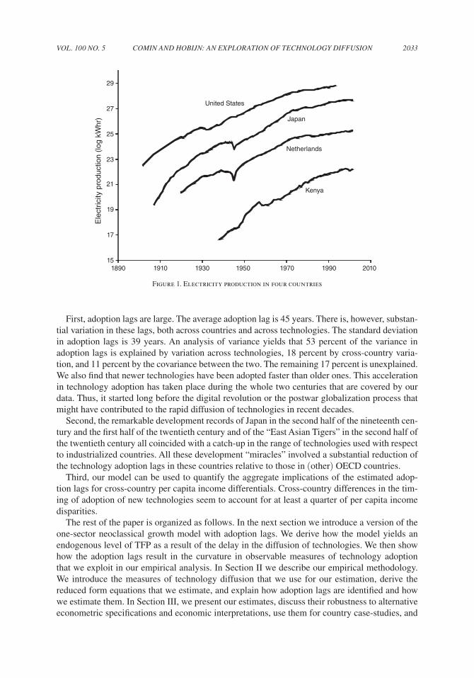
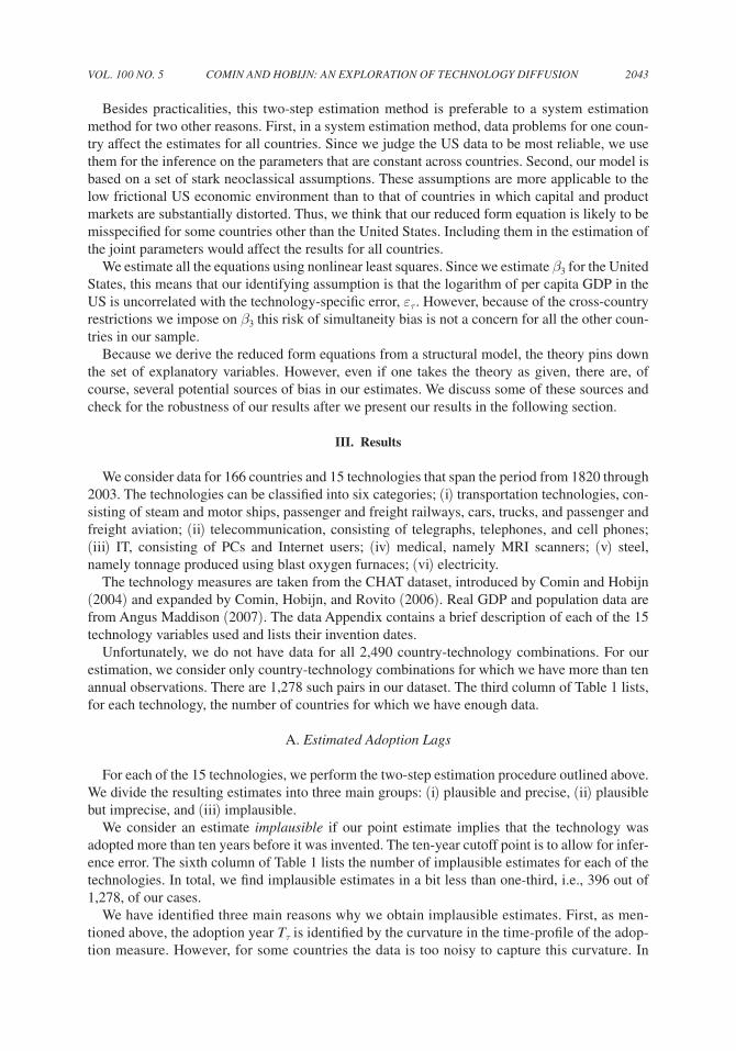
For an example of this curvature, consider Figure 1. It shows the log of kilowatt hours of electric-ity produced over the last 100 years in the United States, Japan, the Netherlands, and Kenya. These curves are roughly the graphic result of shifting a unique curve both horizontally and vertically. This hypothesis is broadly confirmed in a formal test we conduct in Section IVB. According to our model, the horizontal shifts are associated with differences in the lags with which new production methods are adopted in different countries, while vertical shifts reflect many other things including the size of the country and its overall productivity level. The horizontal shifts affect the curvature of the line at each point in time. In particular, our model determines how the curvature of these mea-sures depends on adoption lags and on economy-wide conditions that determine aggregate demand. By using the model predictions about how these factors affect the curvature of these measures of technology diffusion, we identify the adoption lags for each technology and country.

We use data from Comin, Hobijn, and Emilie Rovito (2006) to explore the adoption lags for 15 technologies for 166 countries. Our data cover major technologies related to transportation, tele-communication, IT, health care, steel production, and electricity. We obtain precise and plausible estimates of the adoption lags for two thirds of the 1,278 technology-country pairs for which we have sufficient data. There are three main findings that are especially worth taking away from our exploration.

VOL. 100 NO. 5 2033cOmIN AND HOBIJN: AN ExpLORATION Of TEcHNOLOgy DIffusION

First, adoption lags are large. The average adoption lag is 45 years. There is, however, substan-tial variation in these lags, both across countries and across technologies. The standard deviation in adoption lags is 39 years. An analysis of variance yields that 53 percent of the variance in adoption lags is explained by variation across technologies, 18 percent by cross-country varia-tion, and 11 percent by the covariance between the two. The remaining 17 percent is unexplained. We also find that newer technologies have been adopted faster than older ones. This acceleration in technology adoption has taken place during the whole two centuries that are covered by our data. Thus, it started long before the digital revolution or the postwar globalization process that might have contributed to the rapid diffusion of technologies in recent decades.

Second, the remarkable development records of Japan in the second half of the nineteenth cen-tury and the first half of the twentieth century and of the “East Asian Tigers” in the second half of the twentieth century all coincided with a catch-up in the range of technologies used with respect to industrialized countries. All these development “miracles” involved a substantial reduction of the technology adoption lags in these countries relative to those in (other) OECD countries.

Third, our model can be used to quantify the aggregate implications of the estimated adop-tion lags for cross-country per capita income differentials. Cross-country differences in the tim-ing of adoption of new technologies seem to account for at least a quarter of per capita income disparities.

The rest of the paper is organized as follows. In the next section we introduce a version of the one-sector neoclassical growth model with adoption lags. We derive how the model yields an endogenous level of TFP as a result of the delay in the diffusion of technologies. We then show how the adoption lags result in the curvature in observable measures of technology adoption that we exploit in our empirical analysis. In Section II we describe our empirical methodology. We introduce the measures of technology diffusion that we use for our estimation, derive the reduced form equations that we estimate, and explain how adoption lags are identified and how we estimate them. In Section III, we present our estimates, discuss their robustness to alternative econometric specifications and economic interpretations, use them for country case-studies, and

United States

Japan

Netherlands

Kenya

29

27

25

23

21

19

17

151890 1910 1930 1950 1970 1990 2010

Ele

ctric

ity p

rodu

ctio

n (lo

g kW

hr)

Figure 1. Electricity production in four countries


quantify their implications for cross-country TFP differentials. In Section IV, we conclude by presenting directions for future research. Two Appendices follow. One contains the details of our data and the other the main mathematical derivations.3

I. A One-Sector Growth Model with Adoption Lags

The one-sector model that we introduce here serves two purposes. First, we use it to illustrate how endogenous adoption lags result in endogenous TFP differentials. Second, we use it to show how adoption lags yield curvature in the TFP level of new technologies. This curvature trans-lates into nonlinearities in the time-path of observable measures of technology diffusion that we exploit for our empirical analysis. In what follows, we omit the time subscript, t, where obvious.

A. preferences

A measure one of households populate the economy. They inelastically supply one unit of labor every instant, earn the real wage rate W, and derive the following utility from their con-sumption flow

(1) u = ∫ 0 ∞

e−ρt ln(ct ) dt.

Here ct denotes per capita consumption and ρ is the discount rate. We further assume that capital markets are perfectly competitive and that consumers can borrow and lend at the real rate ̃ r .

The resulting optimal savings decision yields the Euler equation which implies that the growth rate of consumption equals the difference between the real rate and the discount rate. The initial level of consumption is pinned down by the household’s lifetime budget constraint.

B. Technology

final goods production.—Final output, y, is produced competitively by combining a continuum of intermediate goods, indexed by v. Output of each intermediate good, yv, is produced by com-bining labor and capital, Kv , that embodies a specific production method that we call a technology vintage (or vintage) in the following Cobb-Douglas form:

(2) yv = Zv L v 1−α K v

α .

Productivity embodied in each vintage is captured by the variable Zv and is constant over time.Each instant, a new production method appears exogenously, such that the set of vintages

available at time t is given by _

V = (−∞, t ]. The embodied productivity of new vintages grows at a rate γ across vintages, such that

(3) Zv = Z0 eγ v.

This characterizes the evolution of the world technology frontier.

3 Additional mathematical details are provided in an online Appendix.


A country does not necessarily use all the capital vintages that are available in the world because, as we discuss below, making them available for production is costly. The set of vintages actually used is given by V = (−∞, t − D ]. Here D ≥ 0 denotes the adoption lag. That is, the amount of time between when the best technology in use in the country became available and when it was adopted.

We consider a technology to be a set of production methods used to produce closely related intermediates. In particular, in the context of our model, we consider two technologies: an old one, denoted by o, and a new one, denoted by n. The old technology consists of the production methods introduced up till a fixed time _ v , such that the set of vintages associated with the old technology is Vo = (−∞, _ v ]. The new technology consists of the newest production methods, invented after _ v , such that it covers Vn = [ _ v , t ].

Final output is competitively produced using a CES production function of the form:

(4) y = ( ∑ τ∈{o, n}

y τ 1/μ )

μ

, where yτ = ( ∫ Vτ

y v 1/μ dv )

μ

.

To accommodate derivations below, we define associated TFP aggregates as:

(5) A = ( ∑ τ∈{o, n}

A τ 1/μ−1 )

μ−1

, where Aτ = ( ∫ Vτ

Z v 1/μ−1 dv )

μ−1

.

capital goods production and Technology Adoption.—Capital goods are produced by monopo-listic competitors. Each of them holds the patent of the capital good used for a particular produc-tion method. It takes one unit of final output to produce one unit of capital of any vintage. This production process is assumed to be fully reversible. For simplicity, we assume that there is no physical depreciation of capital. The capital goods suppliers rent out their capital goods at the rental rate Rv.

Technology Adoption costs.—In order to become the sole supplier of a particular capital vintage, the capital good producer must undertake an investment, in the form of an up-front fixed cost. We interpret this investment as the adoption cost of the production method associated with the capital vintage.

The cost of adopting vintage v at instant t is assumed to be:

(6) Γvt = _

Ψ (1 + b)( Zv _ Zt

) 1+ϑ _ μ−1

( Zt _ At

) 1 _ μ−1

yt , where ϑ > 0.

Here, the constant _

Ψ is the steady-state stock market capitalization to GDP ratio4 and is included for normalization purposes. The parameter b reflects barriers to adoption in the sense of Parente and Prescott (1994). The term ( Zv/Zt )(1+ϑ)/(μ−1) captures the idea that it is more costly to adopt technologies the higher is their productivity relative to the productivity of the frontier technology. The last two terms capture that the cost of adoption is increasing in the market size.

We choose this functional form because, just like the adoption cost function in Parente and Prescott (1994), it yields the existence of an aggregate balanced growth path. As we shall see

4 In particular, _

Ψ = (α/ϵ)[ 1/(ρ + (γ/(μ − 1)))].


below, on this balanced growth path, the value of adopting a technology is also linear in the mar-ket size. As a result, adoption lags are constant, and we can separately identify the intensive and extensive margins of adoption.5

C. factor Demands, Output, and Optimal Adoption

Intermediate goods Demand.—The demand for the output produced with vintage v is:

(7) yv = y(pv ) − μ _ μ−1

, where p = ( ∫

v∈V

p v − 1 _ (μ−1) dv )

−(μ−1)

.

We use the final good as the numeraire good throughout our analysis and normalize its price to p = 1. Labor is homogenous, competitively supplied, and perfectly mobile across sectors. Since yv is produced competitively, its price equals its marginal cost of production. The revenue share of labor is (1 − α) and the rental costs of capital exhaust the remaining revenue.

capital goods Demands and Rental Rates.—The supplier of each capital good recognizes that the rental price he charges for the capital good, Rv, affects the price of the output associated with the capital good and, therefore, its demand, yv. The resulting demand curve faced by the capital good supplier is

(8) Kv = y Z v 1 _ μ−1

(

(1 − α) _ W

) 1−α _ μ−1

( α _ Rv

) ϵ

, where ϵ ≡ 1 + α _ μ − 1 .

Here, ϵ is the constant price elasticity of demand that the capital goods supplier faces. As a result, the profit maximizing rental price equals a constant markup times the marginal production cost of a unit of capital.

Because of the durability of capital and the reversibility of its production process, the per-period marginal production cost of capital is the user-cost of capital. Thus, the rental price that maximizes the profits accrued by the capital good producer is

(9) Rv = R = ϵ _ ϵ − 1 ̃ r ,

where ϵ/(ϵ − 1) is the constant gross markup factor.

Aggregate Output and Inputs.—We obtain the following aggregate production function representation:

(10) y = AK αL1−α , where K ≡ ∫ −∞

t

Kv dv and L ≡ ∫ −∞

t

Lv dv .

Just as for the underlying capital vintage specific outputs, the labor share is (1 − α) and the capital share is the rest.

5 It could of course be the case that the linearity in the adoption cost function is violated for some particular technol-ogy for some particular country, without necessarily violating balanced growth, but to the extent that we are document-ing adoption lags across many technologies this is perhaps not so critical.


Optimal Adoption.—The flow profits that the capital goods producer of vintage v earns are equal to

(11) πv = α _ ϵ pv yv = α _ ϵ ( Zv _ A ) 1 _ μ−1

y .

The market value of each capital goods supplier equals the present discounted value of the flow profits. That is,

(12) mv,t = ∫ t ∞

e − ∫t s ̃ r s′ ds′ πvs ds = ( Zv _ Zt

) 1 _ μ−1

( Zt _ At

) 1 _ μ−1

Ψt yt .

Here

(13) Ψt = α _ ϵ ∫ t ∞

e − ∫t s ̃ r s′ ds′ ( At _ As

) 1 _ μ−1

( ys _ yt

) ds

is the stock market capitalization to GDP ratio.6

Optimal adoption implies that, every instant, all the vintages for which the value of the firm that produces the capital good is at least as large as the adoption cost will be adopted. That is, for all vintages, v, that are adopted at time t,

(14) Γv ≤ mv .

This holds with equality for the best vintage adopted if there is a positive adoption lag.7

The adoption lag that results from this condition equals

(15) Dv = max { μ − 1 _ γ ϑ {ln (1 + b) − ln Ψ + ln

_ Ψ }, 0} = D

and is constant across vintages, v. At this point it is important to distinguish between two types of factors: the ones that don’t affect adoption lags and the ones that do.

First, given the specifications of the production function and the cost of adoption, the market size symmetrically affects the benefits and costs of adoption. Hence, variation in market size does not affect the timing of adoption, i.e., the adoption lags. Note also that, since on the balanced growth path Ψ =

_ Ψ , the steady-state adoption lags do not depend on aggregate TFP or GDP for

the same reason. As we shall see below, these variables and others that affect the market size do affect how many units of a specific vintage are demanded once it has been adopted, i.e., the intensity of adoption.

Second, factors that distort the returns to capital, such as taxes on the rental price of capital, taxes on the operating profits of capital goods producers, or the expropriation risk they face by the government all affect adoption lags and can be interpreted as being captured by b.8

6 This can be interpreted as the stock market capitalization if all monopolistic competitors are publicly traded companies.

7 If the frontier vintage, t, is adopted and there is no adoption lag then Γtτ ≤ mtτ . For simplicity, we ignore the possi-bility that, for the best vintages, already adopted Γvτ > mvτ . In that case, no new vintages are adopted. This possibility is included in the mathematical derivations in the online Appendix.

8 We illustrate this point with a detailed mathematical example in the online Appendix.


The resulting aggregate TFP level equals

(16) At = A0 eγ (t−Dt ),

where A0 > 0 is a constant that depends on the model parameters.9 Hence, aggregate TFP in this model is endogenously determined by the adoption lags induced by the barriers to entry.

Moreover, the total adoption costs across all vintages adopted at instant t equal

(17) Γ = _

Ψ (1 + b)( γ _ μ − 1 ) e

− ϑ _ μ−1 γD

y (1 − · D ),

where · D denotes the time derivative of the adoption lags.

D. Equilibrium and Diffusion of the New Technology

The equilibrium path of the aggregate resource allocation in this economy can be defined in terms of the following eight equilibrium variables: {c, K, I, Γ, y, A, D, V }. Just as in the standard neoclassical growth model, the capital stock, K, is the only state variable. The eight equations that determine the equilibrium dynamics of this economy are given by:

(i) The consumption Euler equation.

(ii) The aggregate resource constraint10

(18) y = c + I + Γ.

(iii) The capital accumulation equation

(19) · K = −δK + I.

(iv) The production function, (10), taking into account that in equilibrium L = 1.

(v) The adoption cost function, (17).

(vi) The technology adoption equation, (15), that determines the adoption lag.

(vii) The stock market to GDP ratio, (13).

(viii) The aggregate TFP level, (16).

The steady state growth rate of this economy is γ/(1 − α).11

9 In particular A0 = Z0((μ − 1)/γ ) μ−1.10 We assume that adoption costs are measured as part of final demand, such that y can be interpreted as GDP.11 We derive the balanced growth path and approximate transitional dynamics of this economy in the online

Appendix.


Diffusion of the new technology.—The focus of our analysis of technology diffusion is not on the aggregates, but rather on the demand for capital goods and the output produced with the produc-tion methods that make up the new technology τ = n.

We can express output produced with technology τ in the following Cobb-Douglas form

(20) yτ = Aτ K τ α L τ

1−α , where Kτ ≡ ∫ v∈Vτ

Kv dv, Lτ ≡ ∫ v∈Vτ

Lv dv,

where Aτ is defined in (5).The price of the intermediate good equals the marginal cost of production, which is given by

(21) pτ = 1 _ Aτ

( y _ L ) 1−α

( R _ α ) α

while demand equals

(22) yτ = y (pτ ) − μ _ (μ−1) ,

and the rental cost share of capital is equal to α, such that

(23) RKτ = αpτ yτ .

Most importantly, the endogenous level of TFP for technology τ = n at time t can be expressed as

(24) An = ( μ − 1 _ γ )

μ−1

Z _ v e γ (t−Dt− _ v ) [1 − e − γτ _ μ−1

(t− D t − _ v ) ]

μ−1

.

3 8 embodiment effect variety effect

From this equation, it can be seen that our model introduces two mechanisms by which the adop-tion lags, Dτ , affect the level of TFP in the production of intermediate good τ : (i) the embodiment effect; and (ii) the variety effect.

First, as newer vintages with higher embodied productivity are adopted in the economy, the level of embodied productivity increases. This mechanism is captured by the “embodiment effect” term of (24) which reflects the productivity embodied in the best vintage adopted in the economy.

Second, the range of vintages available for production also affects the level of embodied productivity of the new technology. An increase in the measure of vintages adopted leads to higher productivity through the gains from variety. This is captured by the “variety effect” term in expression (24). In particular, when the number of vintages in use is very small, an increase in this number has a relatively large effect on embodied productivity. As this number increases, the productivity gains from an additional vintage decline. Thus, the variety effect leads to a nonlinear trend in the embodied productivity level.

Hence, adoption lags affect the evolution of the TFP of the new technology. This TFP level in turn determines the relative price of the new technology and, through that, governs the speed of diffusion as well as the shape of its diffusion curve. The curvature of this shape is driven by the


variety effect. Since the measure of varieties adopted depends on the adoption lag, the curvature of the diffusion curve allows us to identify the adoption lag in the data.

II. Empirical Application

Our aim is to estimate the adoption lags for different technology-country pairs. We do so by using the main insight from the one-sector model, namely that adoption lags drive the curvature in our measures of technology diffusion. We have data for more than one technology. We there-fore extend the results above to include many sectors, each adopting a new technology that cor-responds to a technology for which we have data.12 To make our estimation feasible, we assume that the economy is in steady state, such that adoption lags are constant over time. They may differ across countries and technologies, however.

In this section, we describe our measures of technology diffusion, discuss the extension of the one-sector model, derive the reduced form equations, and describe the method we use to estimate these equations.

measures of Diffusion.—The empirical literature on technology diffusion, following the semi-nal contributions of Griliches (1957) and Mansfield (1961), has mainly focused on the analy-sis of the share of potential adopters that have adopted a technology. Such shares capture the extensive margin of adoption. Computing these measures requires micro level data that are not available for many technologies and countries. As a result, over the last 50 years, the diffusion of relatively few technologies in a very limited number of countries has been documented.

Our model allows us to explore its predictions for alternative measures of technology diffusion for which data are more widely available. In particular, we focus on (i) yτ , the level of output of the intermediate good produced with technology τ ; and (ii) Kτ , the capital inputs used in the production of this output.

These variables have two advantages over the traditional measures. First, they are available for a broad set of technologies and countries. Second, they capture the number of units of the new technology that each of the adopters has adopted. This intensive margin is important to understand cross-country differences in adoption patterns. For spindles, for example, Gregory Clark (1987) argues that this margin is key to understanding the difference in labor productivity between India and Massachusetts in the nineteenth century.

One of the key findings of the empirical diffusion literature is that adoption measures that cap-ture only the extensive adoption margin follow an S-shape curve. Our model is broadly consistent with this observation. S-shape curves, however, provide a poor approximation of the evolution of technology measures that incorporate both the extensive and intensive adoption margins (Comin, Hobijn, and Rovito 2008). A natural question is what type of functional form provides a parsi-monious representation of these diffusion curves. Our model provides a candidate representation which is parsimonious and does a satisfactory job fitting the data.

A. Reduced form Equations

To allow for multiple sectors, we use a nested CES aggregator, where θ/(θ − 1) reflects the between-sector elasticity of demand and μ/(μ − 1) is, just as in the one-sector model, the within-sector elasticity of demand. Further, we allow the growth rate of embodied technological change,

12 In a previous version of this paper, i.e., Comin and Hobijn (2008), we derive such an extension in detail.


γτ , and the invention date, _ v τ , to vary across technologies. We denote the technology measures for which we derive reduced form equations by mτ ∈ { yτ , kτ }. Small letters denote logarithms.

By replacing the within sector demand elasticity with the between sector elasticity in the demand equation (22), we obtain the log-linearized demand equation

(25) yτ = y − θ _ θ − 1 pτ .

Combining that with the intermediate goods price (21)

(26) pτ = −α ln α − aτ + (1 − α)(y − l) + αr ,

we obtain the reduced form equation (27) for yτ:

(27) yτ = y + θ _ θ − 1 [ aτ − (1 − α)(y − l) − αr − α lnα ].

Similarly, we obtain the reduced form equation for kτ by combining the log-linear capital demand equation

(28) kτ = ln α + pτ + yτ − r

with (25) and (26). These expressions depend on the adoption lag Dτ , through the effect the lag has on aτ .

They also contain the rental rate, r, for which we do not have data. The constant adoption lags for each country and technology over time that we estimate mean that we assume that the econo-mies are close to steady state and that r is approximately constant over time. Consistent with this, we present our estimates for the case of a constant rental rate, where r is part of the constant term that we estimate.

We could estimate the reduced form equations (27) and (28). However, to a first order approxi-mation, γτ only affects yτ and kτ through a linear trend. More specifically, in the mathematical Appendix, we log-linearize (24) around γτ = 0 to obtain the approximation

(29) aτ ≈ z _ v τ + (μ − 1)ln(t − Tτ) − γτ _ 2 (t − Tτ ),

where Tτ = _ v τ + Dτ is the time that the technology is adopted.In this approximation, the growth rate of embodied technological change, γτ , affects only the

linear trend in aτ . Intuitively, when there are very few vintages in Vτ the growth rate of the num-ber of vintages, i.e., the growth rate of t − Tτ , is very large, and it is this growth rate that drives growth in aτ through the variety effect. Only in the long run, when the growth rate of the number of varieties tapers off, the growth rate of embodied productivity, γτ , becomes the predominant driving force over the variety effect.

Then, as we derive in the mathematical Appendix, the reduced form equation that we estimate is the same for both capital and output measures and is of the form

(30) mτ = β1 + y + β2t + β3((μ − 1)ln(t − Tτ) − (1 − α)(y − l)) + ετ ,


where ετ is the error term. The reduced form parameters are given by the βs. We do not estimate μ and α. Instead, we calibrate μ = 1.3, based on the estimates of the markup in manufacturing from Susanto Basu and John G. Fernald (1997), and α = 0.3 consistent with the postwar US labor share.

B. Identification of Adoption Lags and Estimation procedure

We use the reduced form equations to estimate country-technology-specific adoption lags. For this purpose, we make the following three assumptions: (i) Levels of aggregate TFP, relative investment prices, and units of measurement of the technology measures potentially differ across countries; (ii) growth rates of embodied technological change, the relative price per unit of capi-tal, and of aggregate TFP, are the same across countries; (iii) technology parameters are the same except for the adoption lags.

In order to see how these assumptions translate into cross-country parameter restrictions, we consider which structural parameters affect each of the reduced form parameters. The fixed effect, β1, captures four things: (i) the units of the technology measure; (ii) different TFP levels across countries; (iii) differences in adoption lags; and (iv) the level of the relative price of invest-ment goods, which we have abstracted from in our derivations but would affect capital demand and output levels. Because we assume that these things can vary across countries, we let β1 vary across countries as well. The trend-parameter, β2, is assumed to be constant across countries because it only depends on the output elasticity of capital, α,13 and on the trend in embodied technological change.14 β3 depends only on the technology parameter, θ, and is therefore also assumed to be constant across countries.

Given these cross-country parameter restrictions, the adoption lags, Dτ , are identified in the data through the nonlinear trend component in equation (30), which reflects the variety effect. This is the only term affected by the adoption lag, Dτ . It is also the only term which affects the curvature of mτ after controlling for the effect of observables such as (per capita) income. Specifically, it causes the slope in mτ to monotonically decline in the time since adoption. This is the basis of our empirical identification strategy of Dτ . Intuitively, our model predicts that, everything else equal, if at a given moment in time we observe that the slope in mτ is diminishing faster in one country than another, it must be because the former country has started adopting the technology more recently.

Note that, with this identification scheme, we are not using the level of adoption to identify the adoption lags. The intensive margin of adoption can be measured by the country-technology fixed effect β1 in (30), which is affected by the level of TFP and the relative price of capital. In our model, these factors do not affect the timing of adoption, i.e., the extensive margin, but affect the intensity of adoption instead.

Because the adoption lag is a parameter that enters nonlinearly in (30) for each country, esti-mating the system of equations for all countries together is practically not feasible. Instead, we take a two-step approach. We first estimate equation (30) using only data for the United States. This provides us with estimates of the values of β1 and Dτ for the United States as well as esti-mates of β2 and β3 that should hold for all countries. In the second step, we separately estimate β1 and Dτ , using (30) and conditional on the estimates of β2 and β3 based on the US data, for all the countries in the sample besides the United States.

13 The output elasticity of capital is one minus the labor share. Douglas Gollin (2002) provides evidence that the labor share is approximately constant across countries.

14 In a more general model it also depends on the growth rate of the relative price per unit of capital. This is the rea-son that we do not use the trend parameter β2 to identify the growth rate of embodied technological change in the data.


Besides practicalities, this two-step estimation method is preferable to a system estimation method for two other reasons. First, in a system estimation method, data problems for one coun-try affect the estimates for all countries. Since we judge the US data to be most reliable, we use them for the inference on the parameters that are constant across countries. Second, our model is based on a set of stark neoclassical assumptions. These assumptions are more applicable to the low frictional US economic environment than to that of countries in which capital and product markets are substantially distorted. Thus, we think that our reduced form equation is likely to be misspecified for some countries other than the United States. Including them in the estimation of the joint parameters would affect the results for all countries.

We estimate all the equations using nonlinear least squares. Since we estimate β3 for the United States, this means that our identifying assumption is that the logarithm of per capita GDP in the US is uncorrelated with the technology-specific error, ετ . However, because of the cross-country restrictions we impose on β3 this risk of simultaneity bias is not a concern for all the other coun-tries in our sample.

Because we derive the reduced form equations from a structural model, the theory pins down the set of explanatory variables. However, even if one takes the theory as given, there are, of course, several potential sources of bias in our estimates. We discuss some of these sources and check for the robustness of our results after we present our results in the following section.

III. Results

We consider data for 166 countries and 15 technologies that span the period from 1820 through 2003. The technologies can be classified into six categories; (i) transportation technologies, con-sisting of steam and motor ships, passenger and freight railways, cars, trucks, and passenger and freight aviation; (ii) telecommunication, consisting of telegraphs, telephones, and cell phones; (iii) IT, consisting of PCs and Internet users; (iv) medical, namely MRI scanners; (v) steel, namely tonnage produced using blast oxygen furnaces; (vi) electricity.

The technology measures are taken from the CHAT dataset, introduced by Comin and Hobijn (2004) and expanded by Comin, Hobijn, and Rovito (2006). Real GDP and population data are from Angus Maddison (2007). The data Appendix contains a brief description of each of the 15 technology variables used and lists their invention dates.

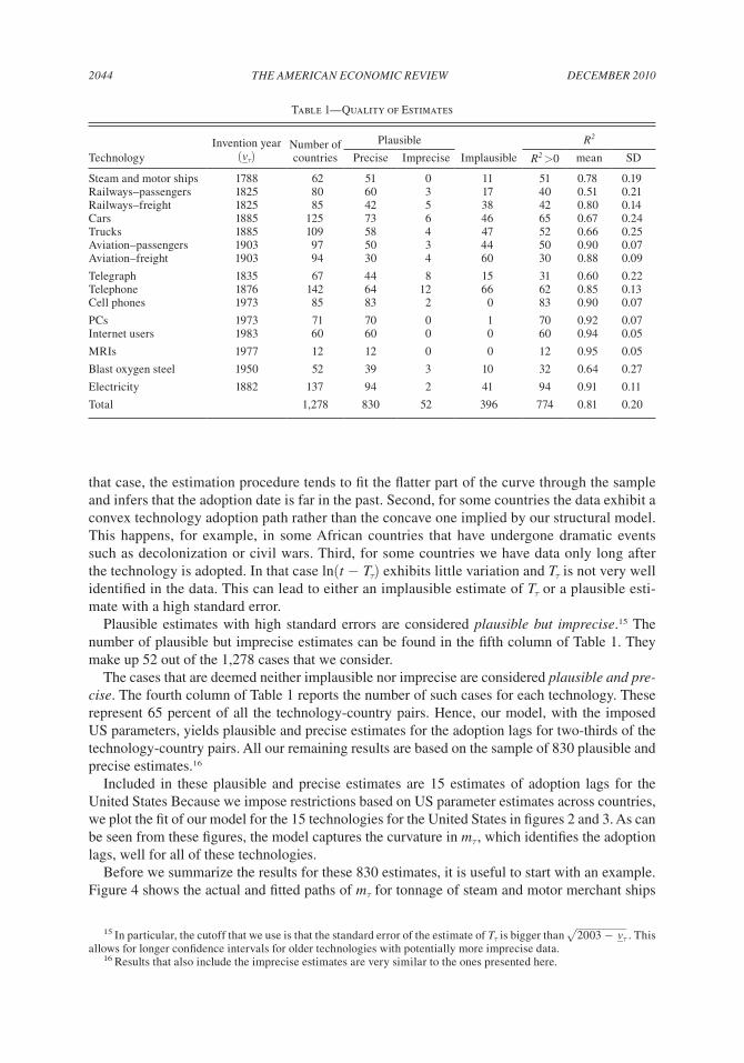
Unfortunately, we do not have data for all 2,490 country-technology combinations. For our estimation, we consider only country-technology combinations for which we have more than ten annual observations. There are 1,278 such pairs in our dataset. The third column of Table 1 lists, for each technology, the number of countries for which we have enough data.

A. Estimated Adoption Lags

For each of the 15 technologies, we perform the two-step estimation procedure outlined above. We divide the resulting estimates into three main groups: (i) plausible and precise, (ii) plausible but imprecise, and (iii) implausible.

We consider an estimate implausible if our point estimate implies that the technology was adopted more than ten years before it was invented. The ten-year cutoff point is to allow for infer-ence error. The sixth column of Table 1 lists the number of implausible estimates for each of the technologies. In total, we find implausible estimates in a bit less than one-third, i.e., 396 out of 1,278, of our cases.

We have identified three main reasons why we obtain implausible estimates. First, as men-tioned above, the adoption year Tτ is identified by the curvature in the time-profile of the adop-tion measure. However, for some countries the data is too noisy to capture this curvature. In


that case, the estimation procedure tends to fit the flatter part of the curve through the sample and infers that the adoption date is far in the past. Second, for some countries the data exhibit a convex technology adoption path rather than the concave one implied by our structural model. This happens, for example, in some African countries that have undergone dramatic events such as decolonization or civil wars. Third, for some countries we have data only long after the technology is adopted. In that case ln(t − T τ ) exhibits little variation and T τ is not very well identified in the data. This can lead to either an implausible estimate of T τ or a plausible esti-mate with a high standard error.

Plausible estimates with high standard errors are considered plausible but imprecise.15 The number of plausible but imprecise estimates can be found in the fifth column of Table 1. They make up 52 out of the 1,278 cases that we consider.

The cases that are deemed neither implausible nor imprecise are considered plausible and pre-cise. The fourth column of Table 1 reports the number of such cases for each technology. These represent 65 percent of all the technology-country pairs. Hence, our model, with the imposed US parameters, yields plausible and precise estimates for the adoption lags for two-thirds of the technology-country pairs. All our remaining results are based on the sample of 830 plausible and precise estimates.16

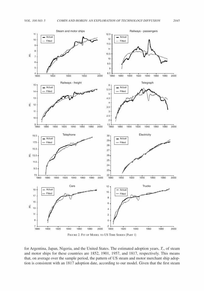
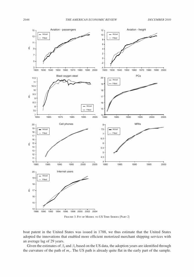
Included in these plausible and precise estimates are 15 estimates of adoption lags for the United States Because we impose restrictions based on US parameter estimates across countries, we plot the fit of our model for the 15 technologies for the United States in figures 2 and 3. As can be seen from these figures, the model captures the curvature in mτ , which identifies the adoption lags, well for all of these technologies.

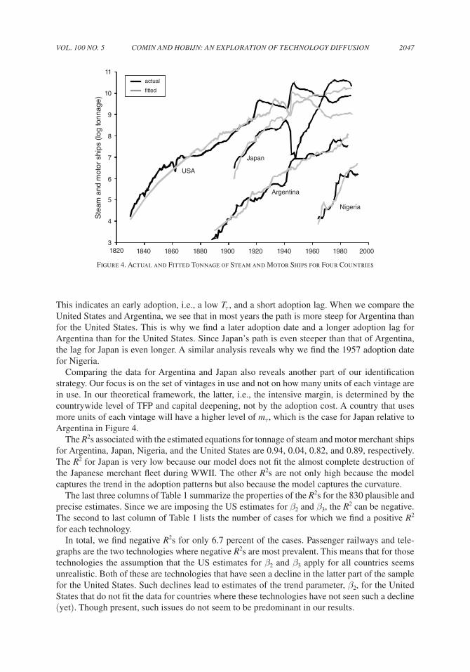
Before we summarize the results for these 830 estimates, it is useful to start with an example. Figure 4 shows the actual and fitted paths of mτ for tonnage of steam and motor merchant ships

15 In particular, the cutoff that we use is that the standard error of the estimate of Tτ is bigger than √ _

2003 − _ v τ . This allows for longer confidence intervals for older technologies with potentially more imprecise data.

16 Results that also include the imprecise estimates are very similar to the ones presented here.

Table 1—Quality of Estimates

Invention year( _ v τ)

Number ofcountries

Plausible R2

Technology Precise Imprecise Implausible R2 >0 mean SD

Steam and motor ships 1788 62 51 0 11 51 0.78 0.19Railways–passengers 1825 80 60 3 17 40 0.51 0.21Railways–freight 1825 85 42 5 38 42 0.80 0.14Cars 1885 125 73 6 46 65 0.67 0.24Trucks 1885 109 58 4 47 52 0.66 0.25Aviation–passengers 1903 97 50 3 44 50 0.90 0.07Aviation–freight 1903 94 30 4 60 30 0.88 0.09

Telegraph 1835 67 44 8 15 31 0.60 0.22Telephone 1876 142 64 12 66 62 0.85 0.13Cell phones 1973 85 83 2 0 83 0.90 0.07

PCs 1973 71 70 0 1 70 0.92 0.07Internet users 1983 60 60 0 0 60 0.94 0.05

MRIs 1977 12 12 0 0 12 0.95 0.05

Blast oxygen steel 1950 52 39 3 10 32 0.64 0.27

Electricity 1882 137 94 2 41 94 0.91 0.11

Total 1,278 830 52 396 774 0.81 0.20


for Argentina, Japan, Nigeria, and the United States. The estimated adoption years, T τ , of steam and motor ships for these countries are 1852, 1901, 1957, and 1817, respectively. This means that, on average over the sample period, the pattern of US steam and motor merchant ship adop-tion is consistent with an 1817 adoption date, according to our model. Given that the first steam

mτ

11

10

9

8

7

6

5

4

12.5

12

11.5

11

10.5

10

9.5

9

8.51800 1850 1900 1950 18602000 1880 1900 1920 1940 1960 1980 2000

Steam and motor ships Railways - passengers

Actual

Fitted

Actual

Fitted

mτ

mτ

mτ

Railways - freight Telegraph

Telephone Electricity

Cars Trucks

Actual

Fitted

Actual

Fitted

Actual

Fitted

Actual

Fitted

Actual

Fitted

Actual

Fitted

1860 1880 1900 1920 1940 1960 1980 2000

1860 1880 1900 1920 1940 1960 1980 2000 1880 1900 1920 1940 1960 1980 2000

1860 1880 1900 1920 1940 1960 1980 2000

15

14

13

12

11

10

9

19.5

17.5

15.5

13.5

11.5

9.5

7.5

12

10

8

6

4

2

0

-2

19

17

15

13

11

9

7

30

29

28

27

26

25

24

23

22

6

5.5

5

4.5

4

3.5

3

2.5

2

1.5

1880 1900 1920 1940 1960 1980 2000 1900 1920 1940 1960 1980 2000

Figure 2. Fit of Model to US Time Series (Part 1)


boat patent in the United States was issued in 1788, we thus estimate that the United States adopted the innovations that enabled more efficient motorized merchant shipping services with an average lag of 29 years.

Given the estimates of β2 and β3 based on the US data, the adoption years are identified through the curvature of the path of mτ . The US path is already quite flat in the early part of the sample.

Actual

Fitted

Actual

Fitted

Actual

Fitted

Actual

Fitted

Actual

Fitted

Actual

Fitted

Actual

Fitted

15

13

11

9

7

5

3

20

19

18

17

16

15

14

20

19

18

17

16

15

14

11.5

11

10.5

10

9.5

9

8.5

8

7.5

7

20

19

18

17

16

15

14

13

12

11

10

1920 1930 1940 1950 1960 1970

1980 1985 1990 1995 2000 2005

1955 1965 1975 1985 1995 2005 1980 1985 1990 1995 2000 2005

1980 1985 1990 1995 2000

1980 1990 2000

1988 1990 1992 1994 1996 1998 2000 2002 2004

1920 1930 1940 1950 1960 1970 1980 1990 2000

Aviation - passengers Aviation - freight

Blast oxygen steel PCs

Cell phones

Internet users

MRIs

mτ

mτ

mτ

mτ

12

10

8

6

4

2

0

-2

-4

8

7.5

7

6.5

6

5.5

5

4.5

4

Figure 3. Fit of Model to US Time Series (Part 2)


This indicates an early adoption, i.e., a low T τ , and a short adoption lag. When we compare the United States and Argentina, we see that in most years the path is more steep for Argentina than for the United States. This is why we find a later adoption date and a longer adoption lag for Argentina than for the United States. Since Japan’s path is even steeper than that of Argentina, the lag for Japan is even longer. A similar analysis reveals why we find the 1957 adoption date for Nigeria.

Comparing the data for Argentina and Japan also reveals another part of our identification strategy. Our focus is on the set of vintages in use and not on how many units of each vintage are in use. In our theoretical framework, the latter, i.e., the intensive margin, is determined by the countrywide level of TFP and capital deepening, not by the adoption cost. A country that uses more units of each vintage will have a higher level of mτ , which is the case for Japan relative to Argentina in Figure 4.

The R2s associated with the estimated equations for tonnage of steam and motor merchant ships for Argentina, Japan, Nigeria, and the United States are 0.94, 0.04, 0.82, and 0.89, respectively. The R2 for Japan is very low because our model does not fit the almost complete destruction of the Japanese merchant fleet during WWII. The other R2s are not only high because the model captures the trend in the adoption patterns but also because the model captures the curvature.

The last three columns of Table 1 summarize the properties of the R2s for the 830 plausible and precise estimates. Since we are imposing the US estimates for β2 and β3, the R2 can be negative. The second to last column of Table 1 lists the number of cases for which we find a positive R2 for each technology.

In total, we find negative R2s for only 6.7 percent of the cases. Passenger railways and tele-graphs are the two technologies where negative R2s are most prevalent. This means that for those technologies the assumption that the US estimates for β2 and β3 apply for all countries seems unrealistic. Both of these are technologies that have seen a decline in the latter part of the sample for the United States. Such declines lead to estimates of the trend parameter, β2, for the United States that do not fit the data for countries where these technologies have not seen such a decline (yet). Though present, such issues do not seem to be predominant in our results.

USA

Japan

Argentina

Nigeria

11

10

9

8

7

6

5

4

31820 1840 1860 1880 1900 1920 1940 1960 1980 2000

Ste

am a

nd m

otor

shi

ps (

log

tonn

age)

actual

�tted

Figure 4. Actual and Fitted Tonnage of Steam and Motor Ships for Four Countries


The next to last and last columns of Table 1 list the sample mean and standard deviations of the distributions of positive R2s for each technology. Overall, the average R2, conditional on being positive, is 0.81 and the standard deviation of these R2s is 0.20. Hence, even though we impose US estimates for β2 and β3 across all countries, the simple reduced form equation, (30), derived from our model captures the majority of the variation in mτ over time for the bulk of the country-technology combinations in our sample.

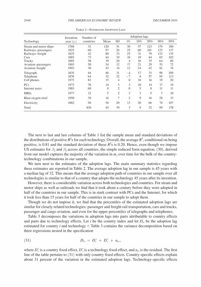
We turn next to the estimates of the adoption lags. The main summary statistics regarding these estimates are reported in Table 2. The average adoption lag in our sample is 45 years with a median lag of 32. This means that the average adoption path of countries in our sample over all technologies is similar to that of a country that adopts the technology 45 years after its invention.

However, there is considerable variation across both technologies and countries. For steam and motor ships as well as railroads we find that it took about a century before they were adopted in half of the countries in our sample. This is in stark contrast with PCs and the Internet, for which it took less than 15 years for half of the countries in our sample to adopt them.

Though we do not impose it, we find that the percentiles of the estimated adoption lags are similar for closely related technologies: passenger and freight rail transportation, cars and trucks, passenger and cargo aviation, and even for the upper percentiles of telegraphs and telephones.

Table 3 decomposes the variations in adoption lags into parts attributable to country effects and parts due to technology effects. Let i be the country index and let Diτ be the adoption lag estimated for country i and technology τ. Table 3 contains the variance decomposition based on three regressions nested in the specification

(31) Diτ = D i * + D τ * + uiτ ,

where D i * is a country fixed effect, D τ * is a technology fixed effect, and uiτ is the residual. The first line of the table pertains to (31) with only country fixed effects. Country-specific effects explain about 31 percent of the variation in the estimated adoption lags. Technology-specific effects

Table 2—Estimated Adoption Lags

Invention Number of Adoption lags

Technology year ( _ v τ) countries Mean SD 1% 10% 50% 90% 99%

Steam and motor ships 1788 51 120 51 30 57 123 179 180Railways–passengers 1825 60 97 26 25 60 101 125 137Railways–freight 1825 42 80 33 25 31 79 123 135Cars 1885 73 44 19 10 19 44 65 102Trucks 1885 58 39 20 4 16 35 64 89Aviation–passengers 1903 50 34 12 17 21 29 53 72Aviation–freight 1903 30 43 14 12 24 42 61 74

Telegraph 1835 44 46 31 −4 17 33 98 109Telephone 1876 64 52 32 − 7 8 57 95 113Cell phones 1973 83 15 4 0 10 16 19 20

PCs 1973 70 14 3 3 10 14 17 19Internet users 1983 60 8 2 0 5 8 11 11

MRIs 1977 12 5 2 3 3 5 7 10

Blast oxygen steel 1950 39 16 7 2 9 16 28 33

Electricity 1882 94 56 20 13 20 66 74 107

Total 830 45 39 3 9 32 99 178


explain about twice as much, namely 65 percent, of the variation. This can be seen from the sec-ond row of Table 3, which is computed from a version of regression (31) with only technology fixed effects. The last row of Table 3 shows that country and technology fixed effects jointly explain about 83 percent of the variation in the estimated adoption lags. Of this, 18 percent can be directly attributed to country effects, 53 percent can be directly attributed to technology effects, and the remaining 12 percent is due to the covariance between these effects that is the result of the unbalanced nature of the panel structure of our data.

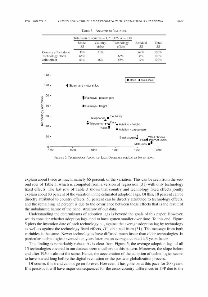
Understanding the determinants of adoption lags is beyond the goals of this paper. However, we do consider whether adoption lags tend to have gotten smaller over time. To this end, Figure 5 plots the invention date of each technology, _ v τ , against the average adoption lag by technology as well as against the technology fixed effects, D τ * , obtained from (31). The message from both variables is the same. Newer technologies have diffused much faster than older technologies. In particular, technologies invented ten years later are on average adopted 4.3 years faster.

This finding is remarkably robust. As is clear from Figure 5, the average adoption lags of all 15 technologies covered in our dataset seem to adhere to this pattern. Moreover, the slope before and after 1950 is almost the same. Hence, the acceleration of the adoption of technologies seems to have started long before the digital revolution or the postwar globalization process.

Of course, this trend cannot go on forever. However, it has gone on at this pace for 200 years. If it persists, it will have major consequences for the cross-country differences in TFP due to the

Steam and motor ships

Railways - passengers

Railways - freight

ElectricityTelephones

Telegrams Cars

TrucksAviation - freight

Aviation - passengers

Blast oxygenPCs

MRI units

Cell phonesInternet users

1750 1800 1850 1900 1950 2000

140

120

100

80

60

40

20

0

Tech

nolo

gy a

dopt

ion

Mean Fixed effect

Figure 5. Technology Adoption Lags Decrease for Later Inventions

Table 3—Analysis of Variance

Total sum of squares = 1,231,426, N = 830

Model SS

Country effect

Technology effect

Residual SS

Total SS

Country effect alone 31% 31% 69% 100%Technology effect 65% 65% 35% 100%Joint effect 83% 18% 53% 17% 100%


lag in technology adoption. In particular, the TFP gap between rich and poor countries due to the lag in technology adoption should be significantly reduced.

Robustness.—Our results are robust to alternative assumptions in the underlying model as long as these do not affect the nonlinear part of equation (30). Most of the relevant variations in the underlying assumptions affect only the interpretation of the intercept (β1 ) and slope (β2 ) parameters which we do not use to identify the adoption lags. For example, as shown in Comin and Hobijn (2008), a model with investment specific technological change yields similar reduced form equations but with a different interpretation of which sources of growth determine the trend. Any distortions that reduce output in the economy at a constant rate over time only affect β1 and do not affect the adoption lag parameter. Capital depreciation and population growth also do not affect the interpretation of β3 and the curvature of the diffusion curves.17

The main assumption we use to identify the adoption lags is that the curvature of the diffusion curve is the same across countries. We explore the empirical validity of this assumption in two ways. For both of these approaches we reestimate equation (30) without imposing the US esti-mate of the curvature parameter, β3, and then compare the unrestricted estimate of β3, which we denote by β 3

u , with the US estimate.First, we formally test whether β3 in each country is equal to that for the United States. Table 4

presents the results of the t-test for the null that β3 = β 3 u in the country-technology pairs where

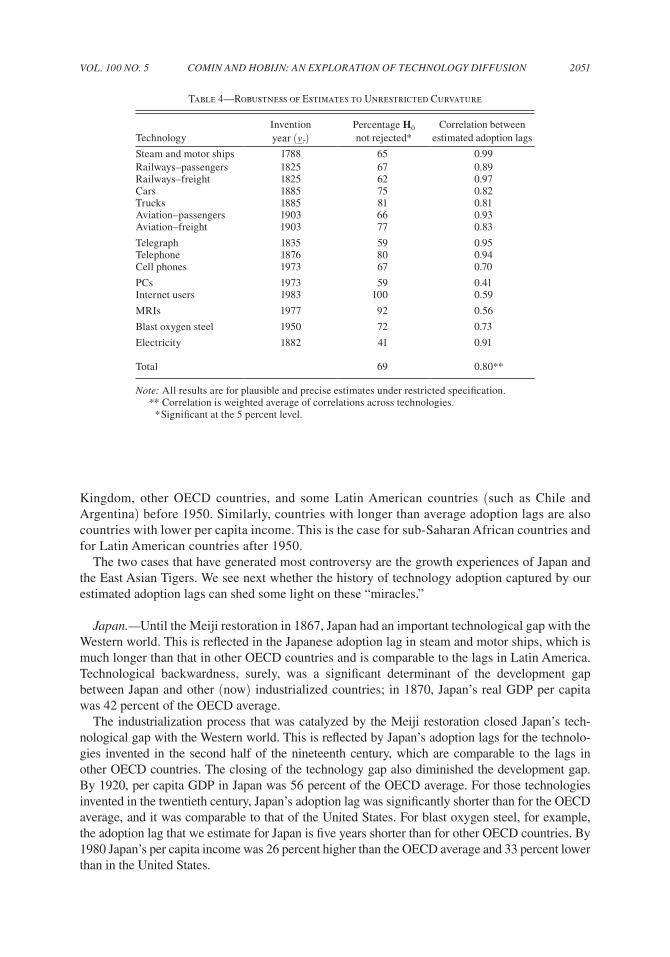
we obtained a plausible and precise estimate of the adoption lags in the restricted estimation. The third column reports, for each technology, the percentage of cases where we cannot reject the null that the curvature is the same as in the United States at a 5 percent significance level. This occurs in 69 percent of the cases.

Second, we compare the adoption lags estimated using the restricted and unrestricted models. This is done in the last column of Table 4. It contains the correlation between the adoption lags estimates from the restricted and unrestricted estimations. The weighted average of the correla-tion across technologies is 0.80. By technologies, the correlations range from 0.41 for computers to 0.99 for steam and motor ships. The conclusion we draw from these results is that allowing for differences in the curvature has little effect on the estimated adoption lags.

In addition to validating our identification assumption, the test reduces the scope for other factors to be significant sources of variation in the curvature of the diffusion curves for our tech-nologies. For example, one could be concerned about the possibility that a reduction in the costs of adoption, say, driven by pro-adoption policies could be generating the curvature. It is however very unlikely that policy changes that, in principle, are independent across countries, led to cur-vatures so similar as the ones observed in the data. Furthermore, these results indicate that our assumption that adoption lags for each technology in a country are relatively constant over time is not rejected in the data.

B. case studies

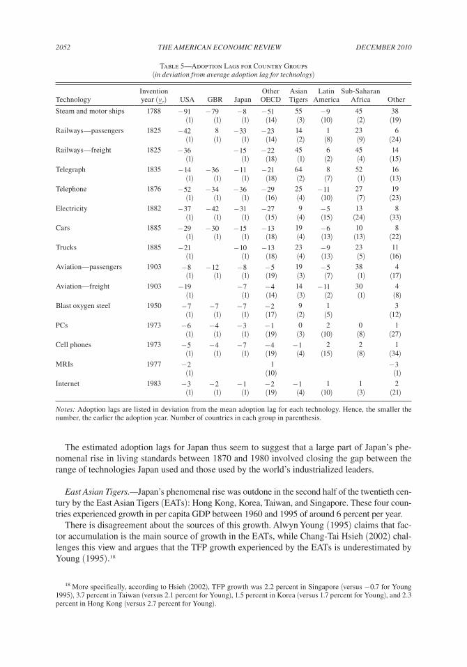
Thus far, we have focused on computing statistics that reflect the broad patterns of technology adoption. Next we explore the estimates in more detail. Table 5 reports, for each technology, the average adoption lag for different groups of countries in deviation from the average adoption lag for the technology.

Consistent with equation (16), countries with high per capita income at one point in time are countries with shorter adoption lags. This is the case of the United States, the United

17 Our estimates turn out to be robust to the calibration of μ and α as well as to the steady-state and log-linear approximations that we applied.


Kingdom, other OECD countries, and some Latin American countries (such as Chile and Argentina) before 1950. Similarly, countries with longer than average adoption lags are also countries with lower per capita income. This is the case for sub-Saharan African countries and for Latin American countries after 1950.

The two cases that have generated most controversy are the growth experiences of Japan and the East Asian Tigers. We see next whether the history of technology adoption captured by our estimated adoption lags can shed some light on these “miracles.”

Japan.—Until the Meiji restoration in 1867, Japan had an important technological gap with the Western world. This is reflected in the Japanese adoption lag in steam and motor ships, which is much longer than that in other OECD countries and is comparable to the lags in Latin America. Technological backwardness, surely, was a significant determinant of the development gap between Japan and other (now) industrialized countries; in 1870, Japan’s real GDP per capita was 42 percent of the OECD average.

The industrialization process that was catalyzed by the Meiji restoration closed Japan’s tech-nological gap with the Western world. This is reflected by Japan’s adoption lags for the technolo-gies invented in the second half of the nineteenth century, which are comparable to the lags in other OECD countries. The closing of the technology gap also diminished the development gap. By 1920, per capita GDP in Japan was 56 percent of the OECD average. For those technologies invented in the twentieth century, Japan’s adoption lag was significantly shorter than for the OECD average, and it was comparable to that of the United States. For blast oxygen steel, for example, the adoption lag that we estimate for Japan is five years shorter than for other OECD countries. By 1980 Japan’s per capita income was 26 percent higher than the OECD average and 33 percent lower than in the United States.

Table 4—Robustness of Estimates to Unrestricted Curvature

Invention Percentage H0 Correlation betweenTechnology year ( _ v τ) not rejected* estimated adoption lags

Steam and motor ships 1788 65 0.99Railways–passengers 1825 67 0.89Railways–freight 1825 62 0.97Cars 1885 75 0.82Trucks 1885 81 0.81Aviation–passengers 1903 66 0.93Aviation–freight 1903 77 0.83

Telegraph 1835 59 0.95Telephone 1876 80 0.94Cell phones 1973 67 0.70

PCs 1973 59 0.41Internet users 1983 100 0.59

MRIs 1977 92 0.56

Blast oxygen steel 1950 72 0.73

Electricity 1882 41 0.91

Total 69 0.80**

Note: All results are for plausible and precise estimates under restricted specification. ** Correlation is weighted average of correlations across technologies. * Significant at the 5 percent level.


The estimated adoption lags for Japan thus seem to suggest that a large part of Japan’s phe-nomenal rise in living standards between 1870 and 1980 involved closing the gap between the range of technologies Japan used and those used by the world’s industrialized leaders.

East Asian Tigers.—Japan’s phenomenal rise was outdone in the second half of the twentieth cen-tury by the East Asian Tigers (EATs): Hong Kong, Korea, Taiwan, and Singapore. These four coun-tries experienced growth in per capita GDP between 1960 and 1995 of around 6 percent per year.

There is disagreement about the sources of this growth. Alwyn Young (1995) claims that fac-tor accumulation is the main source of growth in the EATs, while Chang-Tai Hsieh (2002) chal-lenges this view and argues that the TFP growth experienced by the EATs is underestimated by Young (1995).18

18 More specifically, according to Hsieh (2002), TFP growth was 2.2 percent in Singapore (versus −0.7 for Young 1995), 3.7 percent in Taiwan (versus 2.1 percent for Young), 1.5 percent in Korea (versus 1.7 percent for Young), and 2.3 percent in Hong Kong (versus 2.7 percent for Young).

Table 5—Adoption Lags for Country Groups (in deviation from average adoption lag for technology)

TechnologyInvention year ( _ v τ) USA GBR Japan

Other OECD

Asian Tigers

Latin America

Sub-Saharan Africa Other

Steam and motor ships 1788 − 91 − 79 −8 − 51 55 − 9 45 38(1) (1) (1) (14) (3) (10) (2) (19)

Railways—passengers 1825 − 42 8 − 33 − 23 14 1 23 6(1) (1) (1) (14) (2) (8) (9) (24)

Railways—freight 1825 − 36 − 15 − 22 45 6 45 14(1) (1) (18) (1) (2) (4) (15)

Telegraph 1835 − 14 − 36 − 11 − 21 64 8 52 16(1) (1) (1) (18) (2) (7) (1) (13)

Telephone 1876 − 52 − 34 − 36 − 29 25 − 11 27 19(1) (1) (1) (16) (4) (10) (7) (23)

Electricity 1882 − 37 − 42 − 31 − 27 9 − 5 13 8(1) (1) (1) (15) (4) (15) (24) (33)

Cars 1885 − 29 − 30 − 15 − 13 19 − 6 10 8(1) (1) (1) (18) (4) (13) (13) (22)

Trucks 1885 − 21 − 10 − 13 23 − 9 23 11(1) (1) (18) (4) (13) (5) (16)

Aviation—passengers 1903 − 8 − 12 − 8 − 5 19 − 5 38 4(1) (1) (1) (19) (3) (7) (1) (17)

Aviation—freight 1903 − 19 − 7 − 4 14 − 11 30 4(1) (1) (14) (3) (2) (1) (8)

Blast oxygen steel 1950 − 7 − 7 − 7 − 2 9 1 3(1) (1) (1) (17) (2) (5) (12)

PCs 1973 − 6 − 4 − 3 − 1 0 2 0 1(1) (1) (1) (19) (3) (10) (8) (27)

Cell phones 1973 − 5 − 4 − 7 − 4 − 1 2 2 1(1) (1) (1) (19) (4) (15) (8) (34)

MRIs 1977 − 2 1 − 3(1) (10) (1)

Internet 1983 − 3 − 2 − 1 − 2 − 1 1 1 2(1) (1) (1) (19) (4) (10) (3) (21)

Notes: Adoption lags are listed in deviation from the mean adoption lag for each technology. Hence, the smaller the number, the earlier the adoption year. Number of countries in each group in parenthesis.


Whether or not adoption lags show up as TFP or factor accumulation differentials depends on the extent to which capital stock data are quality adjusted. However, what we can say, based on our estimates, is that, just as for Japan, the growth spurt of the EATs has been associated with a substantial reduction in their technology adoption lags.

From Table 5, it is clear that the EATs had long adoption lags for early technologies. In par-ticular, for technologies invented before 1950, the EATs’ adoption lags were often longer than in sub-Saharan Africa, and almost always longer than in Latin America. For newer technologies, however, the EATs’ adoption lags are shorter than in Latin America and sub-Saharan Africa. In fact, EATs adopted technologies invented since 1950 about as fast as OECD countries.

Young (1992) focuses on the sources of growth in Singapore and Hong Kong and argues that the lower TFP growth rate observed in Singapore reflects its faster rate of structural transforma-tion towards the production of electronics and services, which did not allow agents to learn how to efficiently use older technologies. Some of the post-1950 technologies in our dataset such as computers, cell phones, and the Internet are surely significant for the production of both elec-tronics and services. Hence, an implication of Young’s hypothesis would be that the Singaporean adoption lags in these technologies are shorter than in Hong Kong. This is not what we find. Singapore and Hong Kong are estimated to have the same adoption lags in PCs and the Internet, 14 and seven years respectively. Hong Kong is estimated to have adopted cell phones three years earlier than Singapore.

C. Development Accounting

We conclude our analysis by exploring whether the adoption lags that we have estimated are a significant source of cross-country differences in per capita income. To answer this question, we have to approximate the aggregate effect of the estimated adoption lags for the 15 technologies on per capita GDP levels. We do so by using the equilibrium results of our one-sector growth model. If the only source of cross-country differentials in per capita GDP is adoption lags, then, in steady state, the log difference of country i’s level of real GDP per capita with that of the United States is given by

(32) ( yi − l ) − ( yus − l ) = γ _ 1 − α (Dus − Di ),

where γ is the growth rate of aggregate TFP, which is 1.4 percent for the US private business sec-tor during the postwar period.19 We observe the left-hand side of (32) in our data and approximate the right-hand side in the following way. We use γ = 0.014 and α = 0.3, consistent with postwar US data. Moreover, we use the country fixed effects from (31) to approximate Di ≈ D i * . Hence, we assume that the country-specific adoption lags we have estimated for each country using our sample of technologies are representative of the average adoption lags across all the technologies used in production.

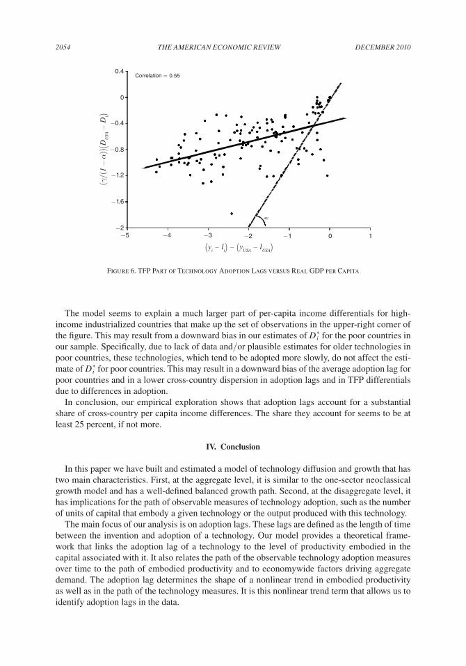
Figure 6 plots the data for both sides of (32) for 123 countries in our dataset. The correlation between the two sides is 0.55. The solid line is the regression line, while the dashed line is the 45-line. The slope of the regression line is about 0.25, which implies that our model and esti-mates explain about one fourth of the log per capita GDP differentials observed in the data.

19 Our empirical analysis is based mostly on technologies that are embodied in physical capital. However, it is rea-sonable to think that there are similar lags in the adoption of disembodied technologies. Hence, our calibration of γ to match overall TFP growth.


The model seems to explain a much larger part of per-capita income differentials for high-income industrialized countries that make up the set of observations in the upper-right corner of the figure. This may result from a downward bias in our estimates of D i * for the poor countries in our sample. Specifically, due to lack of data and/or plausible estimates for older technologies in poor countries, these technologies, which tend to be adopted more slowly, do not affect the esti-mate of D i * for poor countries. This may result in a downward bias of the average adoption lag for poor countries and in a lower cross-country dispersion in adoption lags and in TFP differentials due to differences in adoption.

In conclusion, our empirical exploration shows that adoption lags account for a substantial share of cross-country per capita income differences. The share they account for seems to be at least 25 percent, if not more.

IV. Conclusion

In this paper we have built and estimated a model of technology diffusion and growth that has two main characteristics. First, at the aggregate level, it is similar to the one-sector neoclassical growth model and has a well-defined balanced growth path. Second, at the disaggregate level, it has implications for the path of observable measures of technology adoption, such as the number of units of capital that embody a given technology or the output produced with this technology.

The main focus of our analysis is on adoption lags. These lags are defined as the length of time between the invention and adoption of a technology. Our model provides a theoretical frame-work that links the adoption lag of a technology to the level of productivity embodied in the capital associated with it. It also relates the path of the observable technology adoption measures over time to the path of embodied productivity and to economywide factors driving aggregate demand. The adoption lag determines the shape of a nonlinear trend in embodied productivity as well as in the path of the technology measures. It is this nonlinear trend term that allows us to identify adoption lags in the data.

0.4

0

−0.4

−0.8

−1.2

−1.6

−2−5 −4 −3 −2 −1 0 1

Correlation = 0.55

(yi − l

i) − (yUSA − l

USA)

45°

(γ/(

1 −

α))

(DU

SA −

Di)

Figure 6. TFP Part of Technology Adoption Lags versus Real GDP per Capita


We estimate adoption lags for 15 technologies and 166 countries over the period 1820–2003. Our model does a good job in fitting the diffusion curves. For two thirds of the technology-coun-try pairs we obtain precise and plausible estimates of the adoption lags. In light of this result, we conclude that our model of diffusion provides an empirically relevant micro-foundation for a new set of measures of technology diffusion that are more comprehensive and easier to obtain than the measures used in the traditional empirical diffusion literature.

We obtain three key findings. The first is that adoption lags are large, 45 years on average, and vary a lot. The standard deviation is 39 years. Most of this variation is due to technology-specific variation, which contributes more than half of the variance of adoption lags in our sample. Over the two centuries for which we have data the average adoption lag across countries for new tech-nologies has steadily declined.

The second finding is that the growth “miracles” of Japan and the East Asian Tigers, though more than half a century apart, both coincided with a reduction of the technology adoption lags in these countries relative to those in their OECD counterparts.

Third, when we use our model to quantify the implications of the country-specific variation in adoption lags for cross-country per capita income differentials, we find that differences in technology adoption account for at least a quarter of per capita income disparities in our sample of countries.

Our exploration yields a set of precise estimates of the size of adoption lags across a broad range of technologies and countries. We plan on using these in subsequent work to investigate what are the key cross-country differences in endowments, institutions, and policies that impinge on technology diffusion.

Data Appendix

The data that we use are taken from two sources. Real GDP and population data are taken from Maddison (2007). The data on the technology measure are from the Cross-Country Historical Adoption of Technology (CHAT) dataset, first described in Comin, Hobijn, and Rovito (2006). The 15 particular technology measures, organized by broad category, that we consider are:

1) Steam and motor ships: Gross tonnage (above a minimum weight) of steam and motor ships in use at midyear. Invention year: 1788; the year the first (US) patent was issued for a steam boat design.

2) Railways–Passengers: Passenger journeys by railway in passenger-kilometers. Invention year: 1825; the year of the first regularly scheduled railroad service to carry both goods and passengers.

3) Railways–Freight: Metric tons of freight carried on railways (excluding livestock and passenger baggage). Invention year: 1825; same as passenger railways.

4) Cars: Number of passenger cars (excluding tractors and similar vehicles) in use. Invention year: 1885; the year Gottlieb Daimler built the first vehicle powered by an internal combustion engine.

5) Trucks: Number of commercial vehicles, typically including buses and taxis (excluding tractors and similar vehicles), in use. Invention year: 1885; same as cars.


6) Aviation–Passengers: Civil aviation passenger-kilometers traveled on scheduled ser-vices by companies registered in the country concerned. Invention year: 1903; the year the Wright brothers managed the first successful flight.

7) Aviation–Freight: Civil aviation ton-kilometers of cargo carried on scheduled ser-vices by companies registered in the country concerned. Invention year: 1903; same as aviation–passengers.

8) Telegraph: Number of telegrams sent. Invention year: 1835; year of invention of tele-graph by Samuel Morse at New York University.

9) Telephone: Number of telegrams sent. Invention year: 1876; year of invention of tele-phone by Alexander Graham Bell.

10) Cell phone: Number of users of portable cell phones. Invention year: 1973; first call from a portable cell phone.

11) Personal computers: Number of self-contained computers designed for use by one per-son. Invention year: 1973; first computer based on a microprocessor.

12) Internet users: Number of people with access to the worldwide network. Invention year: 1983; introduction of TCP/IP protocol.

13) MRIs: Number of magnetic resonance imaging (mRI) units in place. Invention year: 1977; first MRI-scanner built.

14) Blast Oxygen Steel: Crude steel production (in metric tons) in blast oxygen furnaces (a process that replaced bessemer and OHF processes). Invention year: 1950; invention of blast oxygen furnace.

15) Electricity: Gross output of electric energy (inclusive of electricity consumed in power stations) in KwHr. Invention year: 1882; first commercial power station on Pearl Street in New York City.

Mathematical Appendix

Derivation of equation (24):This follows from

(33) An = ( ∫ v∈Vn

Z vτ 1 _ μ−1

dv )

μ−1

= ( ∫ _ v t−Dt

( Z _ v e γ (v− _ v ) ) 1 _ μ−1

dv )

μ−1

= Z _ v ( ∫ _ v t−Dt

e

γ _ μ−1 (v− _ v ) dv )

μ−1

= ( μ−1 _ γ )

μ−1

Z _ v e γ (t−Dt− _ v ) [1 − e − γ _ μ−1

(t−Dt− _ v ) ] μ−1

.


Derivation of equation (29):Denote the adoption time by Tτ = Dτ + _ v τ . Consider the technology-specific TFP level

(34) Aτ t = Z _ v τ [( μ − 1 _ γτ ) ( e

γτ _ μ−1

(t−Tτ) − 1) ] μ−1

.

We are interested in the behavior of this TFP for γτ ↓ 0. In that case, there is no embodied pro-ductivity growth, and the increase in productivity after the introduction of the technology is all due to the introduction of an increasing number of varieties over time.

For this reason, we consider

(35) lim γτ↓0

Z _ v τ [( μ − 1 _ γτ

)( e

γτ _ μ−1 (t−Tτ) − 1) ]

μ−1

,

which, using l’Hôpital’s rule, can be shown to equal

(36) Z _ v τ [ lim γτ↓0

( μ − 1 _ γτ

) ( e

γτ _ μ−1 (t−Tτ) − 1)]

μ−1

= Z _ v τ (t − T τ )(μ−1).

Taking the first order Taylor approximation around γ = 0 yields that

(37) Aτ t ≈ Z _ v τ (t − T τ )(μ−1) + Z _ v τ (t − T τ )(μ−2)γτ

× [ lim γτ↓0

(( μ − 1 _ γτ

)(t − T τ ) e

γτ _ μ−1 (t−Tτ) − ( μ − 1

_ γτ )

2

( e

γτ _ μ−1 (t−Tτ) − 1))]

= Z _ v τ (t − Tτ )(μ−1) +

+ Z _ v τ [ lim γτ↓0

( μ − 1 _ γτ

) 2

(( γτ _ μ − 1 (t − T τ ) − 1) e

γτ _ μ−1 (t−Tτ) + 1)](t − T τ )(μ−2)γτ

= Z _ v τ (t − T τ )(μ−1)

+ Z _ v τ [ lim γτ↓0

(μ − 1)2

γτ _ (μ − 1)2

(t − T τ )2 e − γτ _ μ−1

(t−Tτ ) ___

2γτ ] (t − T τ )(μ−2)γτ

= Z _ v τ (t − T τ )(μ−1) + 1 _ 2 Z _ v τ (t − T τ )μγτ

= Z _ v τ (t − T τ )(μ−1) [1 + 1 _ 2 (t − T τ )γτ ] .


Hence, for γτ close to zero,

(38) aτ t ≈ z _ v τ + (μ − 1) ln (t − T τ ) + γτ _ 2 (t − T τ ).

Derivation of equation (30):Combining the four log-linearized equations, we obtain for mτ = yτ that

(39) yτ = y − θ _ θ − 1 pτ

= y + [− θ _ θ − 1 α ln α + θ _ θ − 1

z _ v τ − θ _ θ − 1 γτ _

2 Tτ ]

+ θ _ θ − 1

γτ _ 2 t + θ _ θ − 1

[(μ − 1) ln (t − Tτ ) − (1 − α)(y − l)]

= β1 + y + β2t + β3((μ − 1) ln (t − Tτ ) − (1 − α)(y − l)),

and for mτ = kτ that

(40) kτ = y + ln α − 1 _ θ − 1 pτ − rτ

= [1 + α _ θ − 1 ] ln α + 1 _ θ − 1

[ z _ v τ + γτ _ 2 Tτ ]

+ 1 _ θ − 1 γτ _

2 t + 1 _ θ − 1

[(μ − 1) ln (t − Tτ ) − (1 − α)(y − l)]

= β1 + y + β2 t + β3((μ − 1) ln (t − Tτ ) − (1 − α)(y − l)).

REFERENCES

Basu, Susanto, and John G. Fernald. 1997. “Returns to Scale in US Production: Estimates and Implica-tions.” Journal of political Economy, 105(2): 249–83.

Basu, Susanto, and David N. Weil. 1998. “Appropriate Technology and Growth.” Quarterly Journal of Economics, 113(4): 1025–54.

Caselli, Francesco, and W. John Coleman, II. 2001. “Cross-Country Technology Diffusion: The Case of Computers.” American Economic Review, 91(2): 328–35.

Clark, Gregory. 1987. “Why Isn’t the Whole World Developed? Lessons from the Cotton Mills.” Journal of Economic History, 47(1): 141–73.

Comin, Diego, and Bart Hobijn. 2004. “Cross-Country Technology Adoption: Making the Theories Face the Facts.” Journal of monetary Economics, 51(1): 39–83.

Comin, Diego, and Bart Hobijn. 2008. “An Exploration of Technology Diffusion.” Harvard Business School Working Paper 08-093.

Comin, Diego, Bart Hobijn, and Emilie Rovito. 2006. “Five Facts You Need to Know about Technology Diffusion.” National Bureau of Economic Research Working Paper 11928.

Comin, Diego, Bart Hobijn, and Emilie Rovito. 2008. “A New Approach to Measuring Technology with an Application to the Shape of the Diffusion Curves.” Journal of Technology Transfer, 33(2): 187–207.

Gollin, Douglas. 2002. “Getting Income Shares Right.” Journal of political Economy, 110(2): 458–74.Gort, Michael, and Steven Klepper. 1982. “Time Paths in the Diffusion of Product Innovations.” Economic

Journal, 92(367): 630–53.


Griliches, Zvi. 1957. “Hybrid Corn: An Exploration in the Economics of Technological Change.” Econo-metrica, 25(4): 501–522.

Hall, Robert E., and Charles I. Jones. 1999. “Why Do Some Countries Produce So Much More Output Per Worker than Others?” Quarterly Journal of Economics, 114(1): 83–116.

Hsieh, Chang-Tai. 2002. “What Explains the Industrial Revolution in East Asia? Evidence from the Factor Markets.” American Economic Review, 92(3): 502–26.

Jerzmanowski, Michal. 2007. “Total Factor Productivity Differences: Appropriate Technology Vs. Effi-ciency.” European Economic Review, 51(8): 2080–2110.

Klenow, Peter J., and Andrés Rodríguez-Clare. 1997. “The Neoclassical Revival in Growth Econom-ics: Has It Gone Too Far?” In NBER macroeconomics Annual 1997, ed. Ben S. Bernanke, and Julio J. Rotemberg, 73–103. Cambridge, MA: MIT Press.

Maddison, Angus. 2007. contours of the World Economy, 1–2030 AD: Essays in macro-Economic His-tory. New York: Oxford University Press.

Mansfield, Edwin. 1961. “Technical Change and the Rate of Imitation.” Econometrica, 29(4): 741–66.Manuelli, Rodolfo, and Ananth Seshadri. 2003. “Frictionless Technology Diffusion: The Case of Trac-

tors.” National Bureau of Economic Research Working Paper 9604.Parente, Stephen L., and Edward C. Prescott. 1994. “Barriers to Technology Adoption and Development.”

Journal of political Economy, 102(2): 298–321.Saxonhouse, Gary R., and Gavin Wright. 2004. “Technological Evolution in Cotton Spinning, 1878–

1933.” In The fibre that changed the World: The cotton Industry in International perspective, 1600–1900s, ed. Douglas A. Farnie, and David J. Jeremy, 129–152. New York: Oxford University Press.

Young, Alwyn. 1992. “A Tale of Two Cities: Factor Accumulation and Technical Change in Hong Kong and Singapore.” In NBER macroeconomics Annual 1992, ed. Stanley Fischer, and Olivier Jean Blanchard, 13–54. Cambridge, MA: MIT Press.

Young, Alwyn. 1995. “The Tyranny of Numbers: Confronting the Statistical Realities of the East Asian Growth Experience.” Quarterly Journal of Economics, 110(3): 641–80.

This article has been cited by:

1. John Fernald, , Brent Neiman. 2011. Growth Accounting with Misallocation: Or, Doing Less withMore in SingaporeGrowth Accounting with Misallocation: Or, Doing Less with More in Singapore.American Economic Journal: Macroeconomics 3:2, 29-74. [Abstract] [View PDF article] [PDF withlinks]

2. Badi H. Baltagi, Francesco Moscone, Elisa Tosetti. 2011. Medical technology and the production ofhealth care. Empirical Economics . [CrossRef]

3. Tom Nicholas. 2011. The Origins of Japanese Technological Modernization. Explorations in EconomicHistory . [CrossRef]

4. Diego Comin, Bart Hobijn. 2011. Technology Diffusion and Postwar Growth. NBER MacroeconomicsAnnual 25:1, 209-246. [CrossRef]

http://dx.doi.org/10.1257/mac.3.2.29

http://pubs.aeaweb.org/doi/pdf/10.1257/mac.3.2.29

http://pubs.aeaweb.org/doi/pdfplus/10.1257/mac.3.2.29

http://pubs.aeaweb.org/doi/pdfplus/10.1257/mac.3.2.29

http://dx.doi.org/10.1007/s00181-011-0472-1

http://dx.doi.org/10.1016/j.eeh.2011.01.001

http://dx.doi.org/10.1086/657531

Documents

An Exploration of Technology Diffusion - Dartmouth …dcomin/files/exploration_technology.pdfVOL. 100 NO. 5 cOmIN AND HOBIJN: AN ExpLORATION Of TEcHNOLOgy DIffusION 2033 First, adoption