An Experimental-Design Perspective on Population Ge-netic VariationAndre F. Ribeiro1

1Harvard University, 79 John F. Kennedy St, Cambridge, MA 02138, United States

We consider the hypothesis that Evolution promotes population-wide genome patterns that,under randomization, ensures the External Validity of adaptations across population mem-bers. An adaptation is Externally Valid (EV) if its effect holds under a wide range of popula-tion genetic variations. A prediction following the hypothesis is that pairwise base substitu-tions in segregating regions must be ’random’ as in Erdos-Renyi-Gilbert random graphs, butwith edge probabilities derived from Experimental-Design concepts. We demonstrate theseprobabilities, and consequent mutation rates, in the full-genomes of 2504 humans, 1135 flow-ering plants, 1170 flies, 453 domestic sheep and 1223 brown rats.*

1 Introduction

Whether spontaneous mutations are random is a fundamental and long-standing question in Evo-lutionary Theory and central to our understanding of diseases1–4. As source of genome alterations,patterns in mutations can also help explain the accumulated genetic makeup of organisms. Fewpatterns have however been found, most of them derived from standard population genetics mod-els, such as decreased mutations in deleterious4 and homozygous5 sites. According to standardmodels, such as Wright-Fisher, populations can be represented by two quantities, their size N andmutation rate θ. Genetic variation is then seen as mainly the product of genetic drift (which in-creases genetic variation at random rates) and natural selection (at increased rates). The processes,or population structures, modulating these rates have remained more elusive. There remains littledoubt, however, about their importance. Too large drift can make populations lose many advanta-geous mutants6 or demand too large populations for adaptation. Population structures that improvethe odds of advantageous mutants7 be selected, or reduce deleterious4, can be crucial to popu-lations’ success and survival. The first have been called selection amplifiers and were studiedtheoretically7, 8, when population structures are represented as graphs.

A mutation can increase (or decrease) an individual’s fitness but not do the same for otherpopulation members, possibly sending generations down paths of decreased fitness. Recent re-search in population genetics has investigated the roles that amplifying population structures7,mutation robustness9 and phenotypic diversity10 can have in the evolutionary process. All theseresearch questions can be seen as a questions about phenotypic generalization across populations.It is still unclear which tools from Discrete Mathematics, the Network Sciences and the ComputerSciences are most useful to formulate them. We propose a framework that employs statistical con-

*This research was conducted in 2019.

1

arX

iv:2

108.

0658

0v1

[q-

bio.

PE]

14

Aug

202

1

000

000

1 2

1 2

1 2

a a c

c a b

b a a

time

mut

ant

type

a b c

c a b

b c a

time

a b c

c a b

b c a

time

Low-CF population

Higher-EV population

High-EV, Low-CF population

a) b) c)0

1

2

3

4

0 200 400 600

z (x10

3)

d

...

...

...

...

...... ...

t×S

d)

a b c

c a b

b c a

a b c

c a c

b c c

a b c

c b c

b b c

E[z] = d • pDR

t derangement-pathsof length S

t

d=1 d=2 d=3

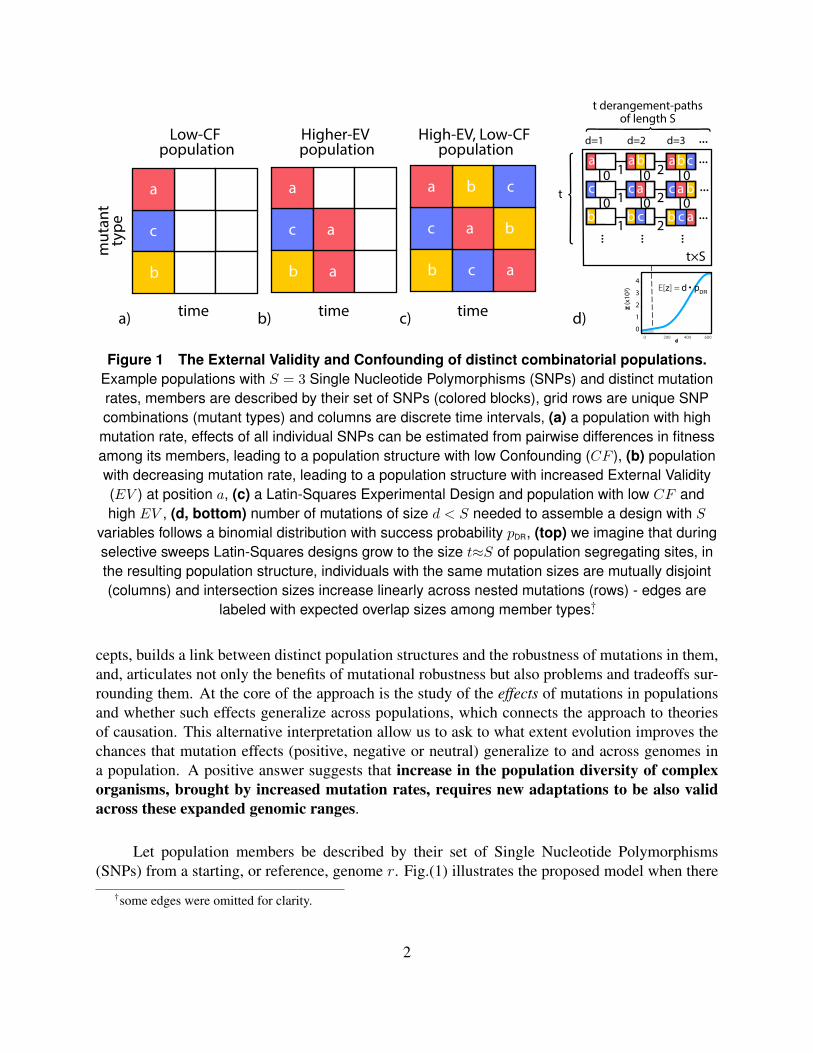
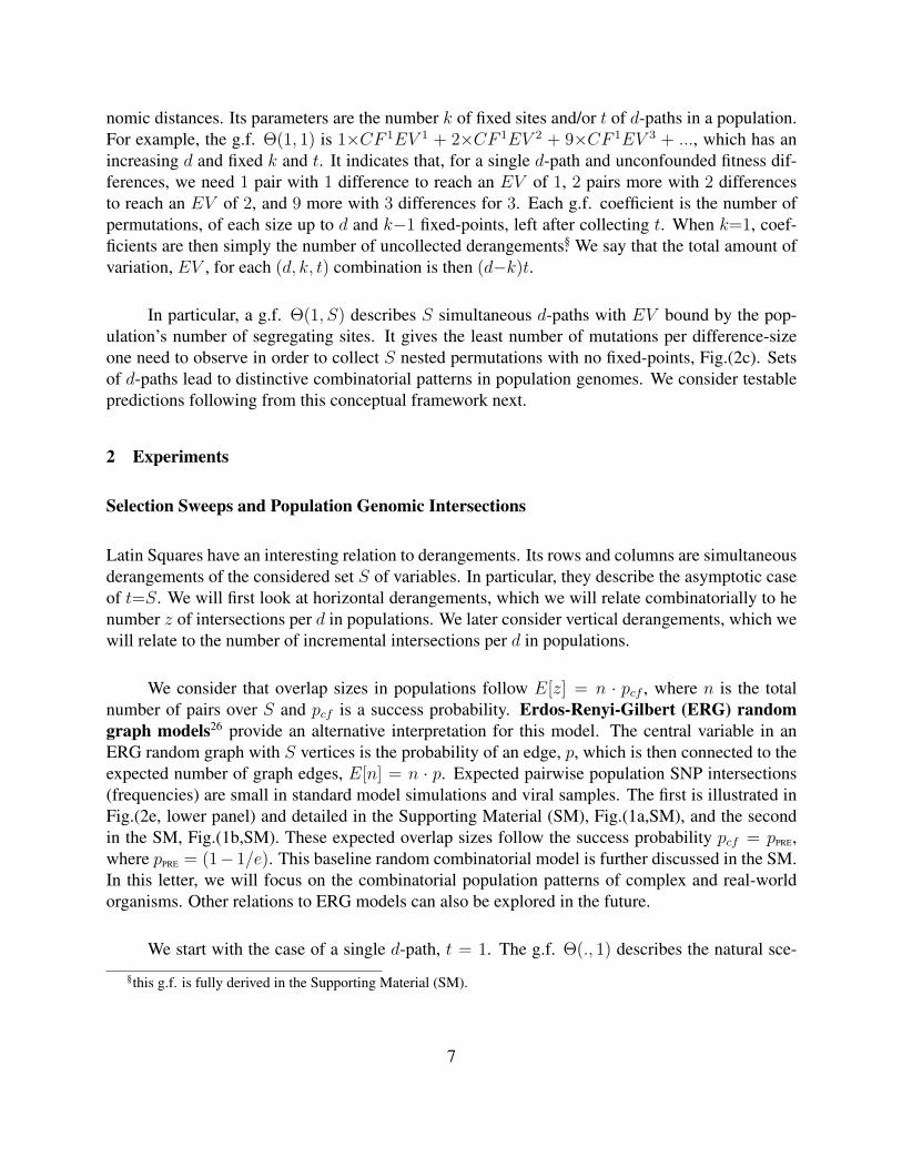
Figure 1 The External Validity and Confounding of distinct combinatorial populations.Example populations with S = 3 Single Nucleotide Polymorphisms (SNPs) and distinct mutationrates, members are described by their set of SNPs (colored blocks), grid rows are unique SNPcombinations (mutant types) and columns are discrete time intervals, (a) a population with highmutation rate, effects of all individual SNPs can be estimated from pairwise differences in fitnessamong its members, leading to a population structure with low Confounding (CF ), (b) populationwith decreasing mutation rate, leading to a population structure with increased External Validity(EV ) at position a, (c) a Latin-Squares Experimental Design and population with low CF andhigh EV , (d, bottom) number of mutations of size d < S needed to assemble a design with S

variables follows a binomial distribution with success probability pDR, (top) we imagine that duringselective sweeps Latin-Squares designs grow to the size t≈S of population segregating sites, inthe resulting population structure, individuals with the same mutation sizes are mutually disjoint(columns) and intersection sizes increase linearly across nested mutations (rows) - edges are

labeled with expected overlap sizes among member types†.

cepts, builds a link between distinct population structures and the robustness of mutations in them,and, articulates not only the benefits of mutational robustness but also problems and tradeoffs sur-rounding them. At the core of the approach is the study of the effects of mutations in populationsand whether such effects generalize across populations, which connects the approach to theoriesof causation. This alternative interpretation allow us to ask to what extent evolution improves thechances that mutation effects (positive, negative or neutral) generalize to and across genomes ina population. A positive answer suggests that increase in the population diversity of complexorganisms, brought by increased mutation rates, requires new adaptations to be also validacross these expanded genomic ranges.

Let population members be described by their set of Single Nucleotide Polymorphisms(SNPs) from a starting, or reference, genome r. Fig.(1) illustrates the proposed model when there

†some edges were omitted for clarity.

2

are S=3 SNPs - labeled a, b and c. Grid columns are time intervals, cells are SNPs and rowsare unique SNP combinations (population mutant types) at the time. Different mutation rates andpopulation structures can make it easy, or impossible, to distinguish fitness gains brought by theseSNPs. If yi is a fitness measure for member i, then fitness differences between any two populationmembers, yi − yj , can reveal the effect of the set of SNPs the two population members differ in.The leftmost population, Fig.(1a), is a population with high mutation rate. At that instant, all SSNPS are added to the current population r. From all resultant pairwise fitness differences amongthis population’s members, we can distinguish the individual effects of all its SNPs. The pairwisegenome differences in this population are {a, b, c}. We say the population has low Confounding(CF ). These effects hold certainly, however, for a limited population (i.e., the one with genome r).On the middle, Fig.(1b), is a population with decreasing mutation rate. In this case, the baselinepopulation where effects hold expands for the SNP labeled a. Effect estimates for a are now pos-sible for populations r, r+b and r+c. We say this population has higher External Validity (EV ).Finally, the rightmost panel shows a Latin-Squares Experimental Design11 . The design is associ-ated with populations whose effects have both maximum EV and minimum CF . Latin Squaresare peculiar in that both their rows and columns are fully pairwise disjoint. Fig.(1d, bottom) showssample sizes required to reproduce these designs under random sampling with replacement (for anincreasing number d of ’variables’). Such concepts will allow us to investigate the mutation ratesevolution chooses compared to those required by such ideal designs, in distinct evolutionaryregimes. A system with expanding EV must sustain a specific mutation rate through time. Suchcases of ’expanding designs’, and their resulting population combinatorial patterns, are illustratedin Fig.(1d, top) and discussed in detail below.

Genetic Combinatorial Patterns

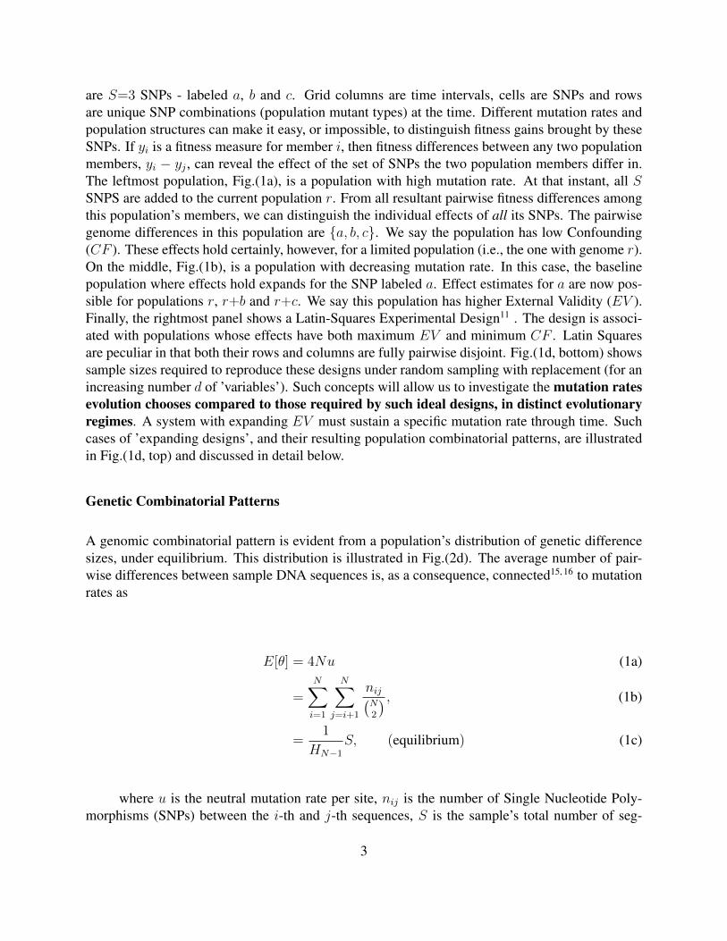
A genomic combinatorial pattern is evident from a population’s distribution of genetic differencesizes, under equilibrium. This distribution is illustrated in Fig.(2d). The average number of pair-wise differences between sample DNA sequences is, as a consequence, connected15, 16 to mutationrates as

E[θ] = 4Nu (1a)

=N∑i=1

N∑j=i+1

nij(N2

) , (1b)

=1

HN−1

S, (equilibrium) (1c)

where u is the neutral mutation rate per site, nij is the number of Single Nucleotide Poly-morphisms (SNPs) between the i-th and j-th sequences, S is the sample’s total number of seg-

3

a)

0

10

20

30

40

0 200 400 600

(x10

3)

n

E[n]

d

S = 500

S = 1.500

S = 10.000

0 200 400 600

d)S = 500

S = 1.500

S = 10.000

e)

E[z] = d • pPRE

n

E[z]

x 1

b)

{ab} {c} {abc}

CF1EV1 CF2EV2 CF3EV3

{a} {bc}

t=1

=

abc

cab

bca

ab

ca

bc

a

c

b

c) (t=1, S=3)

−10000−5000 0 5000 10000

M S

d=1 d=2 d=3

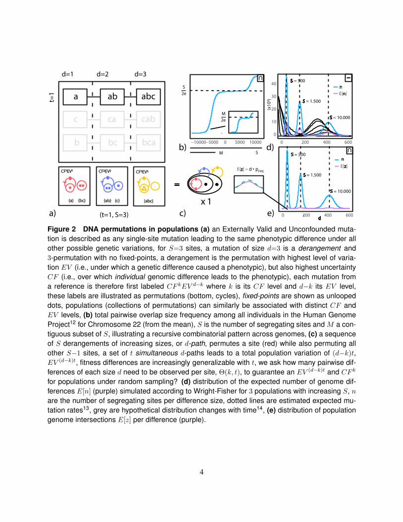
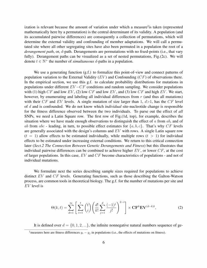
Figure 2 DNA permutations in populations (a) an Externally Valid and Unconfounded muta-tion is described as any single-site mutation leading to the same phenotypic difference under allother possible genetic variations, for S=3 sites, a mutation of size d=3 is a derangement and3-permutation with no fixed-points, a derangement is the permutation with highest level of varia-tion EV (i.e., under which a genetic difference caused a phenotypic), but also highest uncertaintyCF (i.e., over which individual genomic difference leads to the phenotypic), each mutation froma reference is therefore first labeled CF kEV d−k where k is its CF level and d−k its EV level,these labels are illustrated as permutations (bottom, cycles), fixed-points are shown as unloopeddots, populations (collections of permutations) can similarly be associated with distinct CF andEV levels, (b) total pairwise overlap size frequency among all individuals in the Human GenomeProject12 for Chromosome 22 (from the mean), S is the number of segregating sites and M a con-tiguous subset of S, illustrating a recursive combinatorial pattern across genomes, (c) a sequenceof S derangements of increasing sizes, or d-path, permutes a site (red) while also permuting allother S−1 sites, a set of t simultaneous d-paths leads to a total population variation of (d−k)t,EV (d−k)t, fitness differences are increasingly generalizable with t, we ask how many pairwise dif-ferences of each size d need to be observed per site, Θ(k, t), to guarantee an EV (d−k)t and CF k

for populations under random sampling? (d) distribution of the expected number of genome dif-ferences E[n] (purple) simulated according to Wright-Fisher for 3 populations with increasing S, nare the number of segregating sites per difference size, dotted lines are estimated expected mu-tation rates13, grey are hypothetical distribution changes with time14, (e) distribution of populationgenome intersections E[z] per difference (purple).

4

regating sites, and HN−1 is the (N−1)-th harmonic number. Eq.(1c) only holds at equilibrium.Central to the success of these models is their simplicity. Moments for the number of differencesand segregating sites13 have been devised. Further insights into the distribution were proposedby considering their out-of-equilibrium shape (e.g., in the widely popular Tajima D17) and timelyevolution14, 18. The now standard explanation is that population growth leave characteristic signa-tures in the distribution14, as a wave that travels to the right, Fig.(2d, gray). In practice, this is anunsatisfactory explanation however, as natural populations are much more complex, with unknownhistories. Notice that the assumption of random mutations is embedded in Eq.(1) models. Randommutation of DNA sequences with fixed S leads to binomial distributions for their difference sizes.

Fig.(2b) shows the frequency of pairwise overlap sizes among the genomes of all 2504 in-dividuals in the Human Genome Project12 (chromosome 22, from the mean, ordered by size). Itillustrates the prevalence of intersection sizes

[S(e − 1)

]/e2, due to a random combinatorial pat-

tern that repeats for contiguous segregating regions M < S. While Wright-Fisher relate SNPdifferences and mutation rates, Eq.(1b), populations in the model evolve in non-intersecting gen-erations. Patterns in the intersection of populations’ genomes have generally been less scrutinized.SNP intersections in populations are equivalent to their frequency there. According to the viewhere, larger intersections offer the possibility for adaptations’ fitness to be observed under differentlocal genomic, or more general, variations. This leads to adaptations that are not only advanta-geous but also externally valid across the population. Related to issues encountered here, geneticoverlaps have appeared in the study of mutation robustness9, 19, 20. There, robustness is often de-fined as simply the ratio between members with overlapping phenotypes and the total number ofphenotypes in the population. When a large set of mutated genomes observe the same phenotype,mutations are said to be robust. It is, however, unclear why robustness should be important andhow it relates to adaptability and to mutation rates. We make new empirical predictions by consid-ering the statistical consequences of increasing population overlapping genomes, exact forms forthe distribution of overlaps, and a rationale that explains why and how these patterns must changeacross evolutionary regimes.

Model

The main goal of Theoretical Biology is not to describe, but explain, why (and whether) evolutionrequires certain distributions or generative processes, such as randomization. Beyond descriptivesummaries, the distribution of pairwise differences and intersections remain only loosely connectedto the evolutionary process. To that end, we suggest that it is better to think of DNA sequencedifferences in populations as cyclic permutations of DNA subsequences. A pair of memberswith a single nucleotide difference is a permutation of a single site. A pair with d differencespermutes d sites. This is illustrated in Fig.(2a). Permutations are depicted as circles (set of site-nucleotides they permute) and arrows (the bijection and exchanged nucleotides). Non-permutatedelements are called fixed-points and depicted there as unlooped sites. This alternative character-

5

ization is relevant because the amount of variation under which a measure‡is taken (representedmathematically here by a permutation) is the central determinant of its validity. A population (andits accumulated pairwise differences) are consequently a collection of permutations, which willdetermine the external validity and confounding of member adaptations. We will call a permu-tated site where all other segregating sites have also been permuted in a population the root of aderangement path, or, d-path. Derangements are permutations with no fixed-points (i.e., that varyfully). Derangement paths can be visualized as a set of nested permutations, Fig.(2c). We willdenote t ∈ N+ the number of simultaneous d-paths in a population.

We use a generating function (g.f.) to formalize this point-of-view and connect patterns ofpopulation variation to the External Validity (EV ) and Confounding (CF ) of observations there.In the empirical section, we use this g.f. to calculate probability distributions for mutations inpopulations under different EV−CF conditions and random sampling. We consider populationswith (1) high CF and low EV , (2) low CF and low EV , and (3) low CF and high EV . We start,however, by enumerating and labeling all individual differences from r (and thus all mutations)with their CF and EV levels. A single mutation of size larger than 1, d>1, has the CF levelof d and is confounded. We do not know which individual site-nucleotide change is responsiblefor the fitness difference observed between the two individuals. To parse out the effect of allSNPs, we need a Latin Square row. The first row of Fig.(1d, top), for example, describes thesituation where we have made enough observations to distinguish the effect of a from ab, and ofab from abc - leading, in turn, to possible effect estimates for {a, b, c}. That’s why CF levelsare generally associated with the design’s columns and EV with rows. A single Latin square row(t = 1) allow effects to be estimated individually, while multiple rows (t > 1) for individualeffects to be estimated under increasing external conditions. We return to this critical connectionlater (Sect.2 The Connection Between Genetic Derangements and Fitness) but this illustrates thatindividual pairwise differences can be combined to achieve higher EV , or lower CF , at the costof larger populations. In this case, EV and CF become characteristics of populations - and not ofindividual mutations.

We formulate next the series describing sample sizes required for populations to achievedistinct EV and CF levels. Generating functions, such as those describing the Galton-Watsonprocess, are common tools in theoretical biology. The g.f. for the number of mutations per site andEV level is

Θ(k, t) =∞∑d=1

[t∑

i=1

(t

i

)(d!

k!

d∑j=1

(−1)j

j!

)2−i]×CFkEV(d−k)t, (2)

It is defined over d = {0, 1, 2, ...}, the infinite nonnegative natural numbers sequence of ge-‡measures here are fitness differences yi − yj in populations (i.e., the effects of mutations on fitness).

6

nomic distances. Its parameters are the number k of fixed sites and/or t of d-paths in a population.For example, the g.f. Θ(1, 1) is 1×CF 1EV 1 + 2×CF 1EV 2 + 9×CF 1EV 3 + ..., which has anincreasing d and fixed k and t. It indicates that, for a single d-path and unconfounded fitness dif-ferences, we need 1 pair with 1 difference to reach an EV of 1, 2 pairs more with 2 differencesto reach an EV of 2, and 9 more with 3 differences for 3. Each g.f. coefficient is the number ofpermutations, of each size up to d and k−1 fixed-points, left after collecting t. When k=1, coef-ficients are then simply the number of uncollected derangements§. We say that the total amount ofvariation, EV , for each (d, k, t) combination is then (d−k)t.

In particular, a g.f. Θ(1, S) describes S simultaneous d-paths with EV bound by the pop-ulation’s number of segregating sites. It gives the least number of mutations per difference-sizeone need to observe in order to collect S nested permutations with no fixed-points, Fig.(2c). Setsof d-paths lead to distinctive combinatorial patterns in population genomes. We consider testablepredictions following from this conceptual framework next.

2 Experiments

Selection Sweeps and Population Genomic Intersections

Latin Squares have an interesting relation to derangements. Its rows and columns are simultaneousderangements of the considered set S of variables. In particular, they describe the asymptotic caseof t=S. We will first look at horizontal derangements, which we will relate combinatorially to henumber z of intersections per d in populations. We later consider vertical derangements, which wewill relate to the number of incremental intersections per d in populations.

We consider that overlap sizes in populations follow E[z] = n · pcf , where n is the totalnumber of pairs over S and pcf is a success probability. Erdos-Renyi-Gilbert (ERG) randomgraph models26 provide an alternative interpretation for this model. The central variable in anERG random graph with S vertices is the probability of an edge, p, which is then connected to theexpected number of graph edges, E[n] = n · p. Expected pairwise population SNP intersections(frequencies) are small in standard model simulations and viral samples. The first is illustrated inFig.(2e, lower panel) and detailed in the Supporting Material (SM), Fig.(1a,SM), and the secondin the SM, Fig.(1b,SM). These expected overlap sizes follow the success probability pcf = pPRE,where pPRE = (1− 1/e). This baseline random combinatorial model is further discussed in the SM.In this letter, we will focus on the combinatorial population patterns of complex and real-worldorganisms. Other relations to ERG models can also be explored in the future.

We start with the case of a single d-path, t = 1. The g.f. Θ(., 1) describes the natural sce-

§this g.f. is fully derived in the Supporting Material (SM).

7

0e+00

1e+05

2e+05

0 50 100

0

5000

10000

0 50 100 150d

� • pDR

n, total n. of pairs

� • pRND

intersection size, z, frequency

� • pNDR

� • pPRE

0.4 0.5 0.4 0.5 0.2 0.30.4 0.5

0

20000

40000

60000

50 100 150

EAS

AFREUR,SASAMR

0.2 0.3

d

95% HDIpRND

pDR

D = -2.27, D = -0.91 D = -0.88 D = 0.96 D = 3.73 p = 0.02 p = 0.03 p = 0.04 p = 0.03 p = 0.00

pNDR

a) b)

c)D < 0 D > 0

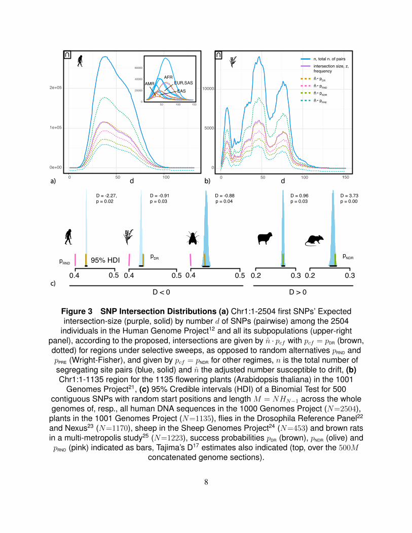
Figure 3 SNP Intersection Distributions (a) Chr1:1-2504 first SNPs’ Expectedintersection-size (purple, solid) by number d of SNPs (pairwise) among the 2504

individuals in the Human Genome Project12 and all its subpopulations (upper-rightpanel), according to the proposed, intersections are given by n · pcf with pcf = pDR (brown,dotted) for regions under selective sweeps, as opposed to random alternatives pRND andpPRE (Wright-Fisher), and given by pcf = pNDR for other regimes, n is the total number ofsegregating site pairs (blue, solid) and n the adjusted number susceptible to drift, (b)Chr1:1-1135 region for the 1135 flowering plants (Arabidopsis thaliana) in the 1001

Genomes Project21, (c) 95% Credible intervals (HDI) of a Binomial Test for 500contiguous SNPs with random start positions and length M = NHN−1 across the wholegenomes of, resp., all human DNA sequences in the 1000 Genomes Project (N=2504),

plants in the 1001 Genomes Project (N=1135), flies in the Drosophila Reference Panel22

and Nexus23 (N=1170), sheep in the Sheep Genomes Project24 (N=453) and brown ratsin a multi-metropolis study25 (N=1223), success probabilities pDR (brown), pNDR (olive) andpRND (pink) indicated as bars, Tajima’s D17 estimates also indicated (top, over the 500M

concatenated genome sections).

8

nario where EV and CF (pairwise differences and intersections) increase together¶. This case wasillustrated in Fig.(2a). Increase of EV (and pairwise intersections) without increase of CF is alsopossible, but it requires larger populations. The g.f. Θ(1, 1) indicates that the number of requiredpairs for each difference size d, where CF remains small, is a series (z1EV

1+z2EV2+...)CF 1.

The resulting coefficients {z1, z2, ...} are associated with a discrete probability distribution func-tion. It’s easy to derive such distribution, notated pDR, by dividing each coefficient by the numberof possible permutations, d!, in each EV level. From Θ(1, 1),

pDR =d!

d!

d∑i=1

(−1)i

i!, (d� k)

≈ 1

e.

(3)

This probability is effectively independent of d. This is due to the known rapid convergence27

of derangements as d increases. It has precision∣∣∣Θ(1,1)

d!−1

e

∣∣∣< 1(d+1)!

, which is under 3 decimals for d

as low as 4. This g.f. stands in contrast to Θ(., 1) which is associated with the known probability27

1/k!e that a random permutation of size d have k sites fixed. This probability is different from pDR

by a fast-increasing margin. Finally, the pairwise sample requirements prescribed by Eq.(2) applyto SNPs that can be lost by drift, which happen with probability 1

HN−1in a given sample. The num-

ber of pairs n = 11− 1

HN−1

n is a sample adjustment similar to drop-out adjustments in Experimental

studies and made by dividing the recommended sample size by the proportion expected not to belost. The expected number of SNP intersections is consequently E[z] = n · pcf where pcf = pDR.

Fig.(3) shows observed mutation intersection counts for two example genomic regions, aswell as credible intervals for binomial tests over 500 random regions across the whole genomes of5 species. The figure shows predictions from n·pDR as well as from alternatives success probabilitiessuch as pPRE and pRND. Empirical observations diverge from these alternatives, as well as from theexpected number of random permutations with k fixed-points, 1/k!e. What is, in fact, observedare numbers very close to the required for populations to increase in EV while keeping CF low.For short, we say we are deranging the population in this case. The similarity between predictedand observed distributions is particularly striking after considering the complexity of evolutionaryevents these populations have undergone. Regions of size M = NHN−1 are used, which arerelevant to the hypothesis that populations are systematically deranged (where N is the samplesize in each case)||.

Tajima’s D estimates across samples, Fig.(3c), indicate that the rate described by pDR is ob-¶for short, we write Θ(., 1) for the series where both d and k follow the N+={1, 2, 3, ...} sequence, k=d.||under drift, the mutation rate is u = 1/4 in this case, Eq.(1a,1c), which is notated pRND for reference.

9

b)1320.50

0.75

0.25

0.50

0.75

1.00

0 20 40 60

imputed population (%)

0 20 40 60

imputed population (%)

0 20 40 60

imputed population (%)a) c) d)

Fd

bottom-up random derangements

0.25

0 20 40 60

imputed population (%)

derangements

0.25

0.25 bottom-up

random

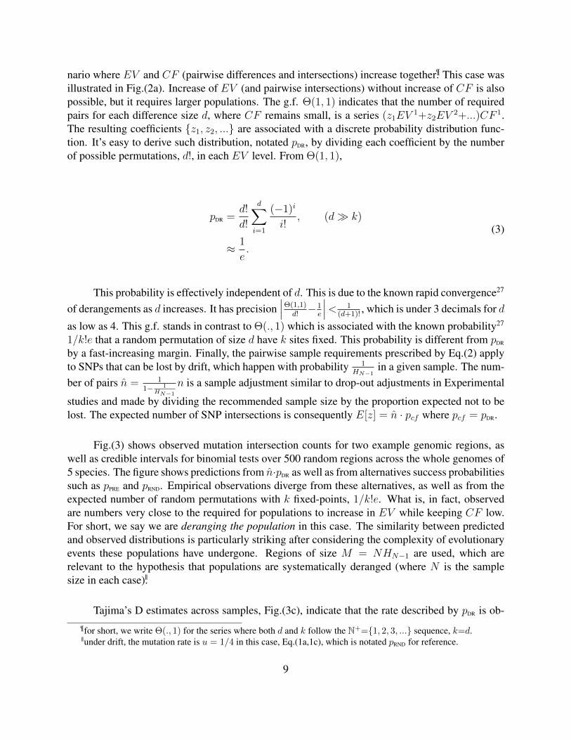
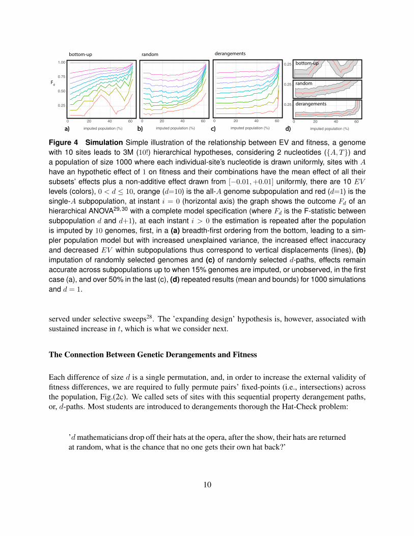
Figure 4 Simulation Simple illustration of the relationship between EV and fitness, a genomewith 10 sites leads to 3M (10!) hierarchical hypotheses, considering 2 nucleotides ({A, T}) anda population of size 1000 where each individual-site’s nucleotide is drawn uniformly, sites with A

have an hypothetic effect of 1 on fitness and their combinations have the mean effect of all theirsubsets’ effects plus a non-additive effect drawn from [−0.01,+0.01] uniformly, there are 10 EV

levels (colors), 0 < d ≤ 10, orange (d=10) is the all-A genome subpopulation and red (d=1) is thesingle-A subpopulation, at instant i = 0 (horizontal axis) the graph shows the outcome Fd of anhierarchical ANOVA29,30 with a complete model specification (where Fd is the F-statistic betweensubpopulation d and d+1), at each instant i > 0 the estimation is repeated after the populationis imputed by 10 genomes, first, in a (a) breadth-first ordering from the bottom, leading to a sim-pler population model but with increased unexplained variance, the increased effect inaccuracyand decreased EV within subpopulations thus correspond to vertical displacements (lines), (b)imputation of randomly selected genomes and (c) of randomly selected d-paths, effects remainaccurate across subpopulations up to when 15% genomes are imputed, or unobserved, in the firstcase (a), and over 50% in the last (c), (d) repeated results (mean and bounds) for 1000 simulationsand d = 1.

served under selective sweeps28. The ’expanding design’ hypothesis is, however, associated withsustained increase in t, which is what we consider next.

The Connection Between Genetic Derangements and Fitness

Each difference of size d is a single permutation, and, in order to increase the external validity offitness differences, we are required to fully permute pairs’ fixed-points (i.e., intersections) acrossthe population, Fig.(2c). We called sets of sites with this sequential property derangement paths,or, d-paths. Most students are introduced to derangements thorough the Hat-Check problem:

’dmathematicians drop off their hats at the opera, after the show, their hats are returnedat random, what is the chance that no one gets their own hat back?’

10

Here, we considered the probability that pairs are deranged in a population corresponds tothe requirement that, in expectation, their common sites are varied. The central concept behindEq.(2) is that the EV of adaptation in populations depends on how many derangements it contains.The minimum number of pairs that guarantees at least one derangement is approximately d/efor a difference of size d. To illustrate the effect of increasing derangements on EV , consider aparticular site, such as the one labeled a in Fig.(1c), and all non-overlapping paths of increasinglengths ending at a in the population. Fig.(1c) shows paths {∅, c, bc}. The sites preceding aare distinct combinations x of other sites. Let fx(a) be the effect (fitness difference) of a, afterx. This is associated with a population pair with intersection x and difference a. We define theEV of a population as the variance of values fx(a), σ2[fx(a)], where each x = {x1, x2, ..., xd}are d sequential derangements of sizes {1, 2, ..., d}. Remember that a permutation of the set ofsegregating sites is a 1-1 mapping of the set onto itself and a derangement is a permutation withno fixed-points, such that no element appears in its original position. The more derangements weobserve, the more variations we measured a site’s effect under, and more confident we are the effectwill generalize to distinct populations.

This points to a curious connection to Game Theory. As an abstract measure, the Shapleyvalue31 (Chap. 17) of an element a of a player-set with size d is the mean payoff difference resultedfrom the addition of a to all its possible subsets. That is, draw a permutation σ ∈ Π(d), eachwith probability 1/d!. Then let players enter a room one-by-one in the order σ and give eachplayer the marginal contribution created by him. Then player a’s payoff is her expected payoffaccording to this repeated random procedure (or its asymptotic ’effect’ given the player-set). Tothe problem at hand, causal effects are related to the expected Shapley value of a variable, whileEV to their variance across the number of observed contexts**. This also implies that total variationincreases with each d-path, for all current simultaneous d-paths, which makes it natural to employa coalitional, or cooperative, concept to understand how joint sample sizes scale.

Fig.(4b-d) describes a simple simulation (see caption) demonstrating these concepts in apopulation with 1000 individuals and 10 segregating sites. It illustrates that maintaining sequen-tial derangements in a population leads to significantly reduced biases in fitness comparisons whencompared to, for example, random and bottom-up genome imputations. In the Supporting Materialand in a concurrent article32, we demonstrate that Machine Learning methods and Causal Effect Es-timators are subject to these same general constraints. The importance of interacting and dependenteffects among SNPs have been demonstrated conclusively by several Genome-Wide AssociationStudies33. Associated with this new outlook on genetics should be Evolutionary mechanisms andstrategies that can deal with these more complex statistical landscapes.

**notice that in this letter we simply equate EV with the level of variation required to estimate it, when using thesame concepts to estimate causal effects32 this more specific definition becomes useful.

11

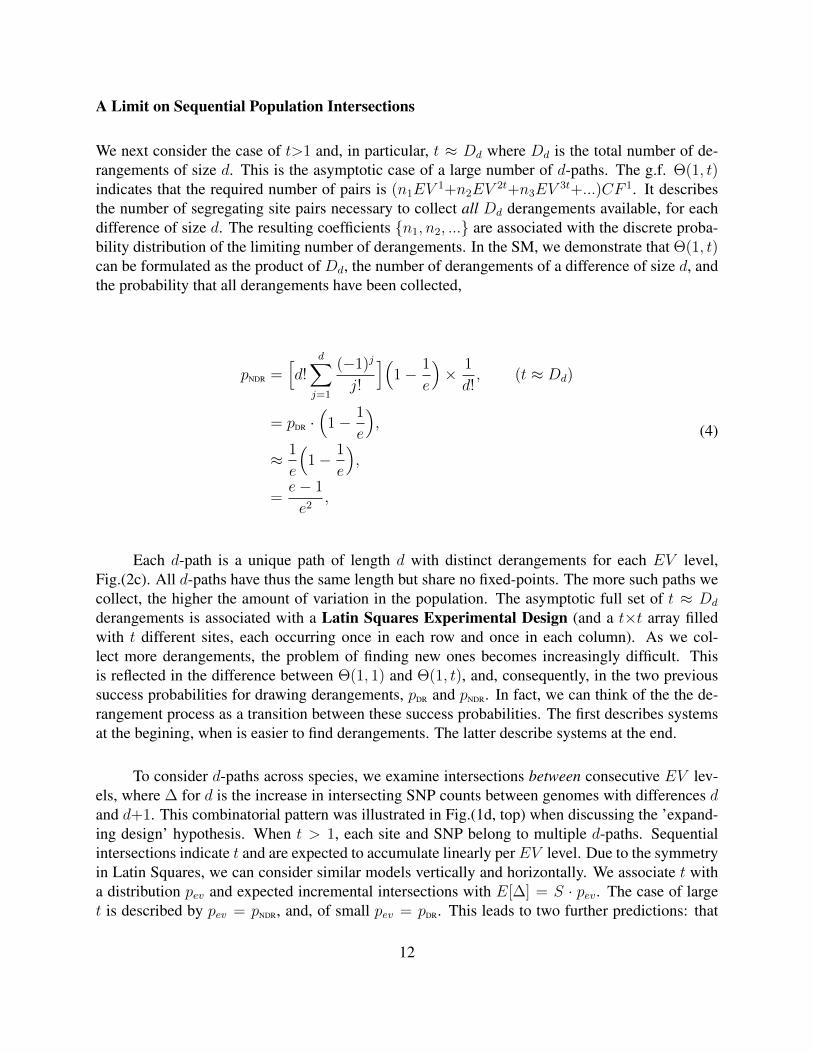
A Limit on Sequential Population Intersections

We next consider the case of t>1 and, in particular, t ≈ Dd where Dd is the total number of de-rangements of size d. This is the asymptotic case of a large number of d-paths. The g.f. Θ(1, t)indicates that the required number of pairs is (n1EV

1+n2EV2t+n3EV

3t+...)CF 1. It describesthe number of segregating site pairs necessary to collect all Dd derangements available, for eachdifference of size d. The resulting coefficients {n1, n2, ...} are associated with the discrete proba-bility distribution of the limiting number of derangements. In the SM, we demonstrate that Θ(1, t)can be formulated as the product of Dd, the number of derangements of a difference of size d, andthe probability that all derangements have been collected,

pNDR =[d!

d∑j=1

(−1)j

j!

](1− 1

e

)× 1

d!, (t ≈ Dd)

= pDR ·(

1− 1

e

),

≈ 1

e

(1− 1

e

),

=e− 1

e2,

(4)

Each d-path is a unique path of length d with distinct derangements for each EV level,Fig.(2c). All d-paths have thus the same length but share no fixed-points. The more such paths wecollect, the higher the amount of variation in the population. The asymptotic full set of t ≈ Dd

derangements is associated with a Latin Squares Experimental Design (and a t×t array filledwith t different sites, each occurring once in each row and once in each column). As we col-lect more derangements, the problem of finding new ones becomes increasingly difficult. Thisis reflected in the difference between Θ(1, 1) and Θ(1, t), and, consequently, in the two previoussuccess probabilities for drawing derangements, pDR and pNDR. In fact, we can think of the the de-rangement process as a transition between these success probabilities. The first describes systemsat the begining, when is easier to find derangements. The latter describe systems at the end.

To consider d-paths across species, we examine intersections between consecutive EV lev-els, where ∆ for d is the increase in intersecting SNP counts between genomes with differences dand d+1. This combinatorial pattern was illustrated in Fig.(1d, top) when discussing the ’expand-ing design’ hypothesis. When t > 1, each site and SNP belong to multiple d-paths. Sequentialintersections indicate t and are expected to accumulate linearly perEV level. Due to the symmetryin Latin Squares, we can consider similar models vertically and horizontally. We associate t witha distribution pev and expected incremental intersections with E[∆] = S · pev. The case of larget is described by pev = pNDR, and, of small pev = pDR. This leads to two further predictions: that

12

0

0 50 100

∆d, intersection size between consecutive EV levels (d,d+1)

0 10 20 30

AFR

EUR,AMR,SAS,EAS

0

100

200

300

0 50 100 150 250 300 350 400

d

Δ

Δ Δ

rug-plot

(μ, σ2) 500 random intervalsa)

b) c)

d) e)d d

∆

∆

∆

0 50 100 150 0 20 40 60

Δ Δ

500

1000

0

250

500

0

50

0

100

0

250

500

S

S

e

e -1e2

( (e -1e2

1e

, ( (1e

1e

,

( (e -1e2

1e

,

SW

BS

EQ

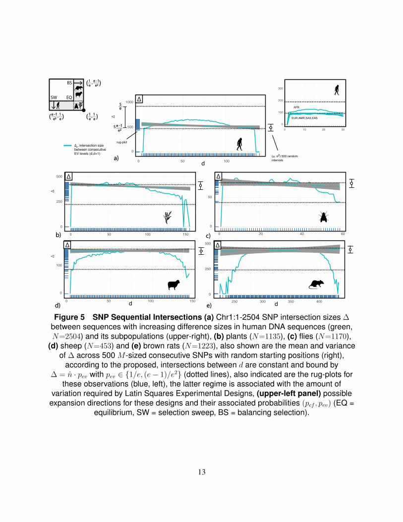
Figure 5 SNP Sequential Intersections (a) Chr1:1-2504 SNP intersection sizes ∆between sequences with increasing difference sizes in human DNA sequences (green,N=2504) and its subpopulations (upper-right), (b) plants (N=1135), (c) flies (N=1170),

(d) sheep (N=453) and (e) brown rats (N=1223), also shown are the mean and varianceof ∆ across 500 M -sized consecutive SNPs with random starting positions (right),

according to the proposed, intersections between d are constant and bound by∆ = n · pev with pev ∈ {1/e, (e− 1)/e2} (dotted lines), also indicated are the rug-plots for

these observations (blue, left), the latter regime is associated with the amount ofvariation required by Latin Squares Experimental Designs, (upper-left panel) possible

expansion directions for these designs and their associated probabilities (pcf , pev) (EQ =equilibrium, SW = selection sweep, BS = balancing selection).

13

intersection increments are constant and take one of two values, pev ∈ [pDR, pNDR]. Furthermore,constant intersection increments naturally lead to ’nested’ subpopulations like the one illustratedin Fig.(2c) (for t=1).

Fig.(5) plots empirical ∆ across species (green). It is hard not to notice how rapidly theseintersection sizes plateau, with a mostly constant ∆. The plateau values also coincide with theprevious limits (dotted lines). Human populations, in particular, have increments described by thelower limit which describe systems with large t. A possible explanation might be the simultane-ous expansion of environmental variation and population (fulfilling both the need and theoreticrequirements for fast increases in EV )34 . This is supported by the distinctive similarity of ∆across all subpopulations, except the African (upper-right panel). Previous results are summa-rized in the upper-left panel in Fig.(5). It depicts the two possible expansion directions (horizontaland vertical) for Latin Square designs, described, in turn, by probabilities (pcf , pev). Equilibrium(EQ, black dot) is characterized by the simultaneous deranging of populations in both directions,(pcf , pev) = (1/e, 1/e). Both derangement types are ’easily’ sampled and have not accumulatedin populations. Selection sweeps (SW) are seen as an acceleration of this same process in onedirection. Systems under SW are described by (pcf , pev) = (1/e, e−1/e2). They have the proposedminimal number of horizontal derangements in populations, but an increasing t (number of d-paths). These are the two conditions formulated for increases in EV with small CF . The reverseis observed for populations under balancing selection.

Conclusion

Here we considered that evolution is not immune to statistical issues familiar to any researcher,and, that it may make strategic use of randomization in response. We looked at mutations, andpopulation genome variation, as DNA permutations and demonstrated that this interpretation andensuing predictions, Eq.(2), lead to distinctive combinatorial patterns across the genomes of 5 ge-netic workhorse species. Each of these patterns places direct constrains on the ranges of observableEukaryote populations.

The biological puzzle of mutations calls for explanations across different levels, such as itsunderlying evolutionary strategies4, resulting population patterns7, 14 and biological mechanisms5, 35.Many other consequences of the EV−CF duality need to be studied, such as its genome, tempo-ral and phylogenic limits. Statistically grounded concepts like External Validity and Confounding(in contrast to more abstract others like mutational robustness9, 19, 20 and graph topologies7, 8) offerrich theoretical possibilities and testable hypotheses when relating population structures to adapt-ability. These concepts could become useful across other evolutionary levels as well. Not justadaptations, as studied, but successful organisms themselves evolve to occupy increasingly variedenvironments, while optimizing their use of the genetic code.

14

References1. Kimura, M. On the evolutionary adjustment of spontaneous mutation rates *. Genetical

Research 9, 23–34 (1967).

2. Levins, R. Theory of fitness in a heterogeneous environment: Part iii. the response to selection.Journal of Theoretical Biology 7, 224–240 (1964).

3. Pal, C., Macia, M. D., Oliver, A., Schachar, I. & Buckling, A. Coevolution with viruses drivesthe evolution of bacterial mutation rates. Nature 450, 1079 (2007).

4. Martincorena, I., Seshasayee, A. S. N. & Luscombe, N. M. Evidence of non-random mutationrates suggests an evolutionary risk management strategy. Nature 485, 95 (2012).

5. Amos, W. Variation in heterozygosity predicts variation in human substitution rates betweenpopulations, individuals and genomic regions.(research article). PLoS ONE 8, e63048 (2013).

6. Mccandlish, D. M., Epstein, C. L. & Plotkin, J. B. Formal properties of the probability offixation: Identities, inequalities and approximations. Theoretical Population Biology 99, 98–113 (2015).

7. Lieberman, E., Hauert, C. & Nowak, M. A. Evolutionary dynamics on graphs. Nature 433,312 (2005).

8. Chastain, E., Livnat, A., Papadimitriou, C. & Vazirani, U. Algorithms, games, and evolution.Proceedings of the National Academy of Sciences 111, 10620 (2014).

9. Draghi, J. A., Parsons, T. L., Wagner, G. P. & Plotkin, J. B. Mutational robustness can facilitateadaptation. Nature (London) 463, 353–355 (2010).

10. Leinonen, T., McCairns, R. J. S., O’Hara, R. B. & Merila, J. Qst–fst comparisons: evolutionaryand ecological insights from genomic heterogeneity. Nature reviews. Genetics 14, 179–190(2013).

11. Mead, R. Statistical Methods in Agriculture and Experimental Biology (CRC Press, 2017).

12. Li, Y. & Consortium, T. . G. P. A global reference for human genetic variation. Nature 526,68 (2015).

13. Fu, Y. X. Statistical properties of segregating sites. Theoretical Population Biology 48, 172–197 (1995).

14. Rogers, A. R. & Harpending, H. Population growth makes waves in the distribution of pairwisegenetic differences. Molecular biology and evolution 9, 552–569 (1992).

15. Watterson, G. A. On the number of segregating sites in genetical models without recombina-tion. Theoretical Population Biology 7, 256–276 (1975).

15

16. Tajima, F. Statistical method for testing the neutral mutation hypothesis by dna polymorphism.Genetics 123, 585–595 (1989).

17. Tajima, F. Evolutionary relationship of dna sequences in finite populations. Genetics 105, 437(1983).

18. Tajima, F. The effect of change in population size on dna polymorphism. Genetics 123,597–601 (1989).

19. Zheng, J., Guo, N. & Wagner, A. Selection enhances protein evolvability by increasing mu-tational robustness and foldability. Science (American Association for the Advancement ofScience) 370 (2020).

20. Fares, M. A. The origins of mutational robustness. Trends in genetics 31, 373–381 (2015).

21. Alonso-Blanco, C. et al. 1,135 genomes reveal the global pattern of polymorphism in ara-bidopsis thaliana. Cell 166, 481–491 (2016).

22. Mackay, T. F. C. et al. The drosophila melanogaster genetic reference panel. Nature 482, 173(2012).

23. Lack, J. B., Lange, J. D., Tang, A. D., Corbett-Detig, R. B. & Pool, J. E. A thousand flygenomes: An expanded drosophila genome nexus. Molecular Biology and Evolution 33,3308–3313 (2016).

24. Alberto, F. et al. Convergent genomic signatures of domestication in sheep and goats. NatureCommunications 9, 813–813 (2018).

25. Combs, M. et al. Urban rat races: spatial population genomics of brown rats (rattus norvegi-cus) compared across multiple cities. Proceedings. Biological sciences 285 (2018).

26. Airoldi, E. M., Goldenberg, A., Zheng, A. & Fienberg, S. A Survey of Statistical NetworkModels, vol. 2 (Springer Verlag, 2009).

27. Hanson, D., Seyffarth, K. & Weston, J. H. Matchings, derangements, rencontres. MathematicsMagazine 56, 224–229 (1983).

28. Sabeti, P. C. Positive natural selection in the human lineage. Science (American Associationfor the Advancement of Science) 312, 1614–1620 (2006).

29. Yang, R. Estimating hierarchical f-statistics. Evolution 52, 950–956 (1998).

30. Goudet, J. hierfstat , a package for r to compute and test hierarchical f -statistics. MolecularEcology Notes 5, 184–186 (2005).

31. Peters, H. Game Theory: A Multi-Leveled Approach (Springer Berlin Heidelberg, Berlin,Heidelberg, 2015).

16

32. Ribeiro, A. Cancer causal polymorphisms have higher-order interactions and effects. (UnderPreparation) (2020).

33. Torkamani, A., Wineinger, N. E. & Topol, E. J. The personal and clinical utility of polygenicrisk scores. Nature Reviews Genetics 19, 581 (2018).

34. Henn, B. M., Cavalli-Sforza, L. L. & Feldman, M. W. The great human expansion. Proceed-ings of the National Academy of Sciences 109, 17758 (2012).

35. Ebersberger, I., Metzler, D., Schwarz, C. & Paabo, S. Genomewide comparison of dna se-quences between humans and chimpanzees. The American Journal of Human Genetics 70,1490–1497 (2002).

17