Embed Size (px)
Citation preview

AN EXPERIMENTAL DESIGN BASED EVALUATION OF
SENSITIVITIES OF MECHANISTIC – EMPIRICAL PAVEMENT DESIGN
GUIDE (MEPDG) PREDICTIONS FOR ONTARIO’S LOCAL
CALIBRATION
Gulfam-E- Jannat, M.A.Sc
PhD Student
Department of Civil and Environmental Engineering
University of Waterloo
Susan L. Tighe, PhD, PEng
Professor
Department of Civil and Environmental Engineering
University of Waterloo
ABSTRACT
A Mechanistic-Empirical Pavement Design Guide (MEPDG) was developed under NCHRP
Project 1-37A to address the shortcomings of empirical pavement design methods. The MEPDG
uses mechanistic-empirical models to analyze the impacts of traffic, climate, materials and
pavement structure and to predict long term performances of pavement. The MEPDG software
(AASHTOWare Pavement M-E) use a three-level hierarchical input scheme to predict pavement
performance in terms of terminal International Roughness Index (IRI), Permanent Deformation ,
Total Cracking (Reflective and Alligator), Asphalt Concrete (AC) Thermal Fracture, AC Bottom-
Up Fatigue Cracking, and AC Top-Down Fatigue Cracking. Different highway agencies are taking
initiatives to adopt MEPDG based pavement design and performance prediction by calibrating the
prediction models for their local conditions. However, these inputs with different levels of
accuracy may have significant impact on performance prediction and thereby on accuracy of local
calibration. This study focuses on the sensitivity of the input parameters of MEPDG distresses to
identify the effect of the accuracy level of input parameters based on orthogonal experimental
design. A local sensitivity analysis is carried out by using Ontario’s default value and historical
performance record of Ontario highway system. Sensitive input parameters are evaluated through
a multiple regression analysis for respective distresses. It is found that terminal IRI is sensitive to
initial IRI, initial permanent deformation, and milled thickness in asphalt layer; permanent
deformation is sensitive to initial permanent deformation, subgrade resilient modulus, and traffic
load; top down fatigue cracking is sensitive to AC effective binder content, and AC air voids.
Based on the independent influence of these sensitive inputs, the requirement of accuracy level
will be identified for MEPDG design.
Key Words: Performance Prediction, MEPDG, Sensitivity, Input Parameters
1. INTRODUCTION
A Mechanistic-Empirical Pavement Design Guide (MEPDG) was developed in the USA under
NCHRP 1-37A in 2004 to address the shortcomings of empirical pavement design methods [1; 2].

1
This MEPDG approach is being adapted by the majority of highway agencies in North America,
to incorporate all possible local factors for traffic, pavement materials and environmental
conditions. MEPDG based distress prediction model incorporates local traffic, pavement materials
and environmental conditions using the mechanistic empirical (M-E) models which will predict
the distresses in a realistic way. Local calibration can further improve accurate prediction
incorporating local conditions. The MEPDG distress models are developed by using Long Term
Pavement Performance (LTPP) data which include pavement sections from many states in the
USA and some provinces in Canada. These models are required to be adjusted for local conditions
using local traffic, climate, material specification and construction activity. For calibration of the
distress prediction models of Ontario highway systems, the historical pavement performance
record from the Ministry of Transportation, Ontario (MTO) Pavement Management System (PMS-
2) database, project specific information from the project documents and default values from the
AASHTOWare Pavement M-E Design Interim Report’ [3] are used are used as input parameters.
The MEPDG based recent software, AASHTOWare Pavement M-E (version-2) allows input data
at three level of accuracy. The local calibration guide [4] suggested using the same accuracy levels
for future design. However, it would be ineffective to put effort for obtaining accuracy of level 1
for all input parameters. For this reason, a sensitivity analysis is essential to identify important
input parameters which have significant impacts on MEPDG distresses.
Several sensitivity analyses have been conducted to address and understand the influential input
parameters of the MEPDG process. NCHRP [5] analyzed five pavement types: new hot-mix
asphalt (HMA), HMA over a stiff foundation, new jointed plain concrete pavement (JPCP), JPCP
over a stiff foundation, and new continuously reinforced concrete pavement (CRCP). In this study
a normalized sensitivity index was adopted as the quantitative metric. NCHRP [6] also carried out
global sensitivity analyses for five pavement types under five climate conditions and three traffic
levels. Retherford and McDonald [7] developed Gaussian process (GP) surrogate models for each
relevant distress mode. The GP models were used for sensitivity analysis and design optimization.
Graves and Mahboub [8] carried out a sampling-based global sensitivity analysis to identify
influential variables of the parameters. Orobio and Zaniewski [9] conducted space-filling computer
experiments with latin hypercube sampling, standardized regression coefficients, and Gaussian
stochastic processes to categorize the relative importance of the material inputs in MEPDG for
flexible pavement. Moya and Prozzi [10] conducted a case study of a pavement structure by
considering several pavement design variables as random. Sensitivity of rutting and other
distresses to input parameters (rutting sensitive to thin layer) are presented for different countries
[11]. The impact of accuracy of traffic input parameters for forecasting traffic loads for pavement
design are also analyzed [12]. MEPDG key input parameters (hot-mix asphalt, base nominal
aggregate size, climate location, HMA thickness, AADTT, subgrade strength, truck traffic
category, construction season, and binder grade are analyzed and impact on major distresses are
discussed using local sensitivity [13]. Siraj et al [14] verified the accuracy of the predicted
performance from the MEPDG software for the state of New Jersey for level 2 and level 3 inputs.
Guclu et al. [15] carried out sensitivity for JPCP and the design input parameters were categorized
as being most sensitive, moderately sensitive, or least sensitive in terms of their relative effect on
distresses .Hall and Beam [16] assessed the relative sensitivity of the models used in the M-E
design guide to inputs relating to portland cement concrete materials of JPCP.

2
The objective of this study is to find the effect of input parameters on MEPDG distresses to identify
the requirement of accuracy level for precise prediction and local calibration. For statistical
validity of investigations, an experimental design based approach is used. Since, orthogonal design
consists of uncorrelated or independent contrasts, economic run size and it ensures fairness in
comparison, this method is considered for experimental design. A multiple linear regression
model is also used for screening the input variables, which has the similar assumption of
independent variables as of orthogonal design. The normalized values (dividing by maximum
value of corresponding variable) of the variables of the regression model readily give the relative
influences of different input parameters on MEPDG distresses.
2. ACCURACY LEVELS OF INPUT DATA
The input data required for the AASHTOWare Pavement M-E analysis are mainly of traffic,
climate, and pavement structure along with materials’ properties. This software allows input data
at three level of accuracy (AASHTO 2014), as described below.
Level 1: Input parameters are the most accurate. Generally, site-specific and laboratory data
or results of actual field testing are considered as level 1 input. For example, laboratory test
values of dynamic modulus, and nonlinear resilient modulus are considered as level 1 for
materials’ properties. For traffic, site specific traffic data (AADTT, lane number, traffic
growth factor etc.) are considered as level 1 input.
Level 2: Generally the input parameters estimated from mathematical correlations or
regression equations, or the calculated from other site specific data are considered as level
2. For example, resilient modulus estimated from CBR values is considered as level 2 input.
Level 3: Input parameters are the least accurate. They are normally default values or based
on best estimates. Generally, national level or regional level values are used.
The level of accuracy and required quality of the input parameters are recommended by
AASHOTO guide for the local calibration of the MEPDG Guide (AASHTO 2010).The input data
are mainly collected from the Ministry of Transportation, Ontario (MTO) Pavement Management
System (PMS-2) database.
3. EXPERIMENTAL DESIGN
A sensitivity analysis will be conducted to investigate relative influences of input parameters.
Generally, sensitivity analysis designs are categorized into three classes: screening methods, local
sensitivity analysis and global sensitivity analysis [8].
Screening method focuses on the hierarchical ranking according to importance of input factors,
rather than providing change in quantity or impact on output. Local sensitivity focuses on the local
impact of the input factors on the performance of output. This method is carried out by varying
certain factor keeping other input factors as constant. Global sensitivity analysis is carried out
varying the input parameter over the entire input parameters.
The input parameters may have the independent and/or combined effects on distress outputs.
Since, the independent influence of an input parameter defines the accuracy level necessary for
that input parameter, local sensitivity will be suitable the method. Local sensitivity will identify
the requirement of higher level of accuracy which is significant step for local calibration especially
for selecting the properties of local materials and traffic. Moreover, orthogonal based design will
investigate independent influence since the experimental sets are independent. So, for the local
calibration an orthogonal design based experimental method will be suitable for this study.
3
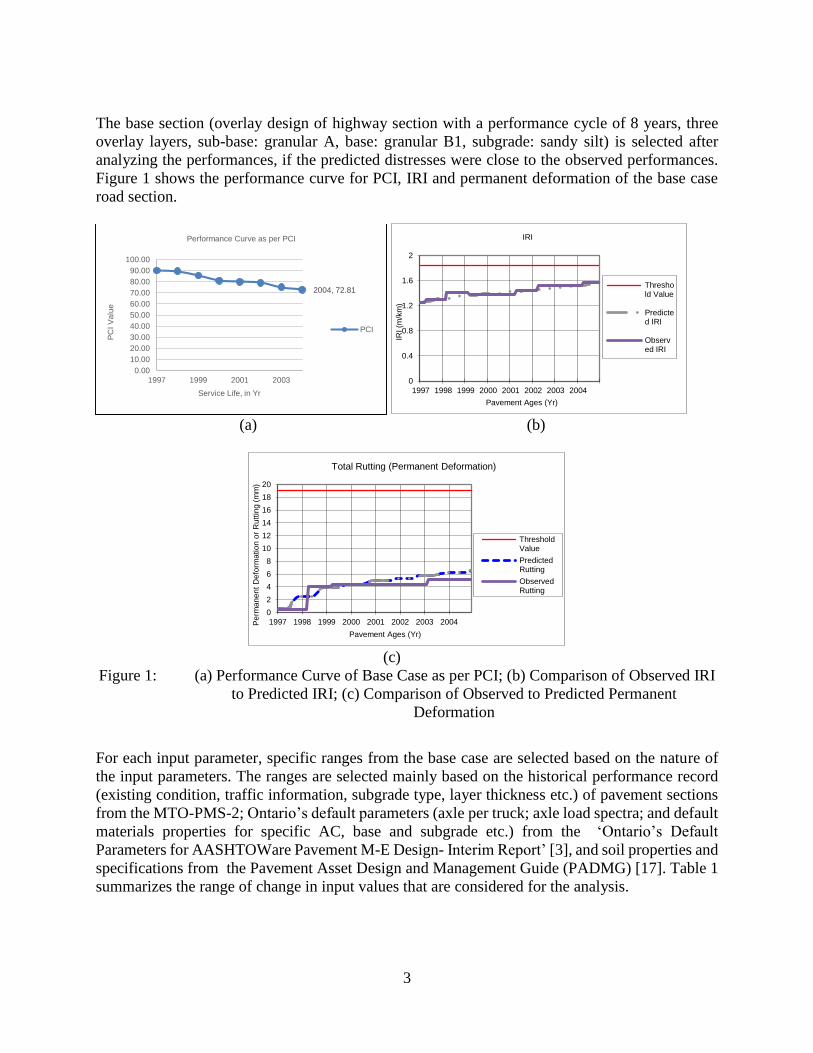
The base section (overlay design of highway section with a performance cycle of 8 years, three
overlay layers, sub-base: granular A, base: granular B1, subgrade: sandy silt) is selected after
analyzing the performances, if the predicted distresses were close to the observed performances.
Figure 1 shows the performance curve for PCI, IRI and permanent deformation of the base case
road section.
(a) (b)
(c)
Figure 1: (a) Performance Curve of Base Case as per PCI; (b) Comparison of Observed IRI
to Predicted IRI; (c) Comparison of Observed to Predicted Permanent
Deformation
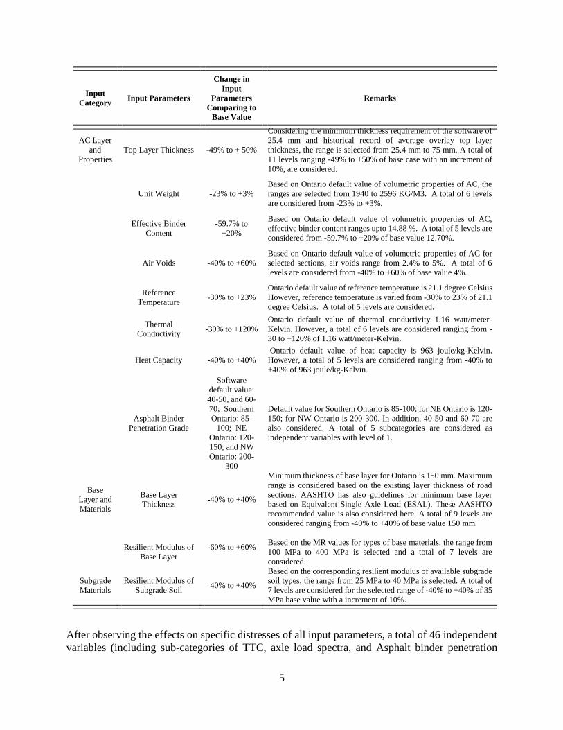
For each input parameter, specific ranges from the base case are selected based on the nature of
the input parameters. The ranges are selected mainly based on the historical performance record
(existing condition, traffic information, subgrade type, layer thickness etc.) of pavement sections
from the MTO-PMS-2; Ontario’s default parameters (axle per truck; axle load spectra; and default
materials properties for specific AC, base and subgrade etc.) from the ‘Ontario’s Default
Parameters for AASHTOWare Pavement M-E Design- Interim Report’ [3], and soil properties and
specifications from the Pavement Asset Design and Management Guide (PADMG) [17]. Table 1
summarizes the range of change in input values that are considered for the analysis.
2004, 72.81
0.00
10.00
20.00
30.00
40.00
50.00
60.00
70.00
80.00
90.00
100.00
1997 1999 2001 2003
PC
I V
alu
e
Service Life, in Yr
Performance Curve as per PCI
PCI
0
0.4
0.8
1.2
1.6
2
1997 1998 1999 2000 2001 2002 2003 2004IR
I (m
/km
)Pavement Ages (Yr)
IRI
Threshold Value
Predicted IRI
Observed IRI
0
2
4
6
8
10
12
14
16
18
20
1997 1998 1999 2000 2001 2002 2003 2004Pe
rma
ne
nt
Defo
rma
tio
n o
r R
utt
ing
(m
m)
Pavement Ages (Yr)
Total Rutting (Permanent Deformation)
ThresholdValue
PredictedRutting
ObservedRutting

4
Table 1: Summary of the Ranges of Input Parameters
Input
Category Input Parameters
Change in
Input
Parameters
Comparing to
Base Value
Remarks
Existing
Condition Initial IRI -40% to + 40%
Considering the target value (1.9 m/km for freeways and 2.3 m/km
for Arterials) of IRI for Ontario, the range of change in initial IRI of
base case is selected. A total of 9 levels are considered from -40%
to +40% with 10% increment.
Initial Permanent
Deformation -50% to + 50%
Considering the target value of Permanent deformation of 19 mm
for Ontario, the range of change in existing permanent deformation
of base case is selected. A total of 11 levels are considered from -
50% to +50% with 10% increment.
Milled Thickness
40 mm to
maximum 100
mm
From the historical record, 40 mm to 100 mm milled thickness are
found. The ranges are selected from 40 mm to 100 mm with
increment of 20 mm. A total of 4 levels are considered.
Traffic
Annual Average
Daily Truck Traffic
(AADTT)
-50% to + 50%
From the historical record of AADTT of all road sections, the ranges
are selected from 700 to 2109 with increment of 10%. A total of 11
levels are considered.
Percent Truck in
Design Lane -25% to + 11%
From the default value of percent of truck in design lane based on
the number of lanes in one direction and AADT in both direction,
the ranges are selected from 60% to 100% with increment of 10%.
A total of 9 levels are considered.
Traffic Growth
Factor -50% to + 50%
From the annual historical record of AADT, the compound growth
factors are calculated for all road sections. The ranges are selected
from 1.65% to 4.94% with increment of 10% which are -50% to
+50% of base case value. A total of 11 levels are considered.
Operational Speed -40% to + 40%
Considering the speed limit of highways, the ranges are selected
from min 60 km to max 140 km with increment of 10% which are -
40% to +40% of base case value. A total of 9 levels are considered.
Axle per Truck
Default Value
of Southern
Ontario,
Northern
Ontario and
Ontario 2006
Default value of Southern Ontario, Northern Ontario and Ontario
2006 value are considered as 3 independent variables with level 1.
Truck Traffic Class
(TTC)
TTC type 1 to
17
Types of TTC are defined based on 17 combination of %bus, %
single trailer truck, and % multi trailer truck. Each type is considered
as an independent variable with level of 1.
Axle Load Spectra
Default Value
of Southern
Ontario,
Northern
Ontario,
Ontario 2006
and Software
Default Value
Based on default value of Southern Ontario, Northern Ontario and
Ontario 2006 value. In addition, software default value is considered
and a total of 4 independent variables each with single level are
considered.
Climate Water Table Depth -60% to + 60%
Based on Ontario default value of 6.1 m, ranges are selected from
2.44 to 9.76 m. A total of 7 levels are considered from -60% to
+60% with a 20% increment.
5
Input
Category Input Parameters
Change in
Input
Parameters
Comparing to
Base Value
Remarks
AC Layer
and
Properties
Top Layer Thickness -49% to + 50%
Considering the minimum thickness requirement of the software of
25.4 mm and historical record of average overlay top layer
thickness, the range is selected from 25.4 mm to 75 mm. A total of
11 levels ranging -49% to +50% of base case with an increment of
10%, are considered.
Unit Weight -23% to +3%
Based on Ontario default value of volumetric properties of AC, the
ranges are selected from 1940 to 2596 KG/M3. A total of 6 levels
are considered from -23% to +3%.
Effective Binder
Content
-59.7% to
+20%
Based on Ontario default value of volumetric properties of AC,
effective binder content ranges upto 14.88 %. A total of 5 levels are
considered from -59.7% to +20% of base value 12.70%.
Air Voids -40% to +60%
Based on Ontario default value of volumetric properties of AC for
selected sections, air voids range from 2.4% to 5%. A total of 6
levels are considered from -40% to +60% of base value 4%.
Reference
Temperature -30% to +23%
Ontario default value of reference temperature is 21.1 degree Celsius
However, reference temperature is varied from -30% to 23% of 21.1
degree Celsius. A total of 5 levels are considered.
Thermal
Conductivity -30% to +120%
Ontario default value of thermal conductivity 1.16 watt/meter-
Kelvin. However, a total of 6 levels are considered ranging from -
30 to +120% of 1.16 watt/meter-Kelvin.
Heat Capacity -40% to +40%
Ontario default value of heat capacity is 963 joule/kg-Kelvin.
However, a total of 5 levels are considered ranging from -40% to
+40% of 963 joule/kg-Kelvin.
Asphalt Binder
Penetration Grade
Software
default value:
40-50, and 60-
70; Southern
Ontario: 85-
100; NE
Ontario: 120-
150; and NW
Ontario: 200-
300
Default value for Southern Ontario is 85-100; for NE Ontario is 120-
150; for NW Ontario is 200-300. In addition, 40-50 and 60-70 are
also considered. A total of 5 subcategories are considered as
independent variables with level of 1.
Base
Layer and
Materials
Base Layer
Thickness -40% to +40%
Minimum thickness of base layer for Ontario is 150 mm. Maximum
range is considered based on the existing layer thickness of road
sections. AASHTO has also guidelines for minimum base layer
based on Equivalent Single Axle Load (ESAL). These AASHTO
recommended value is also considered here. A total of 9 levels are
considered ranging from -40% to +40% of base value 150 mm.
Resilient Modulus of
Base Layer
-60% to +60%
Based on the MR values for types of base materials, the range from
100 MPa to 400 MPa is selected and a total of 7 levels are
considered.
Subgrade
Materials
Resilient Modulus of
Subgrade Soil -40% to +40%
Based on the corresponding resilient modulus of available subgrade
soil types, the range from 25 MPa to 40 MPa is selected. A total of
7 levels are considered for the selected range of -40% to +40% of 35
MPa base value with a increment of 10%.
After observing the effects on specific distresses of all input parameters, a total of 46 independent
variables (including sub-categories of TTC, axle load spectra, and Asphalt binder penetration

6
grade as independent variables) are considered for the analysis. The levels of the parameter values
are found to be different for each independent input variable since the ranges of the levels are
different. Finally, an experimental design is used to identify a total of 171 experimental sets
considering 46 independent variables. The variables are normalized so that the results can be
compared readily.
4. RESULT ANALYSIS
For these experiments, distresses are predicted by using the AASHTOWare Pavement M-E. The
predicted values of each distress are compared to the corresponding target values of failure which
are shown in Table 2. The rate of changes in output distresses are compared. The rate of changes
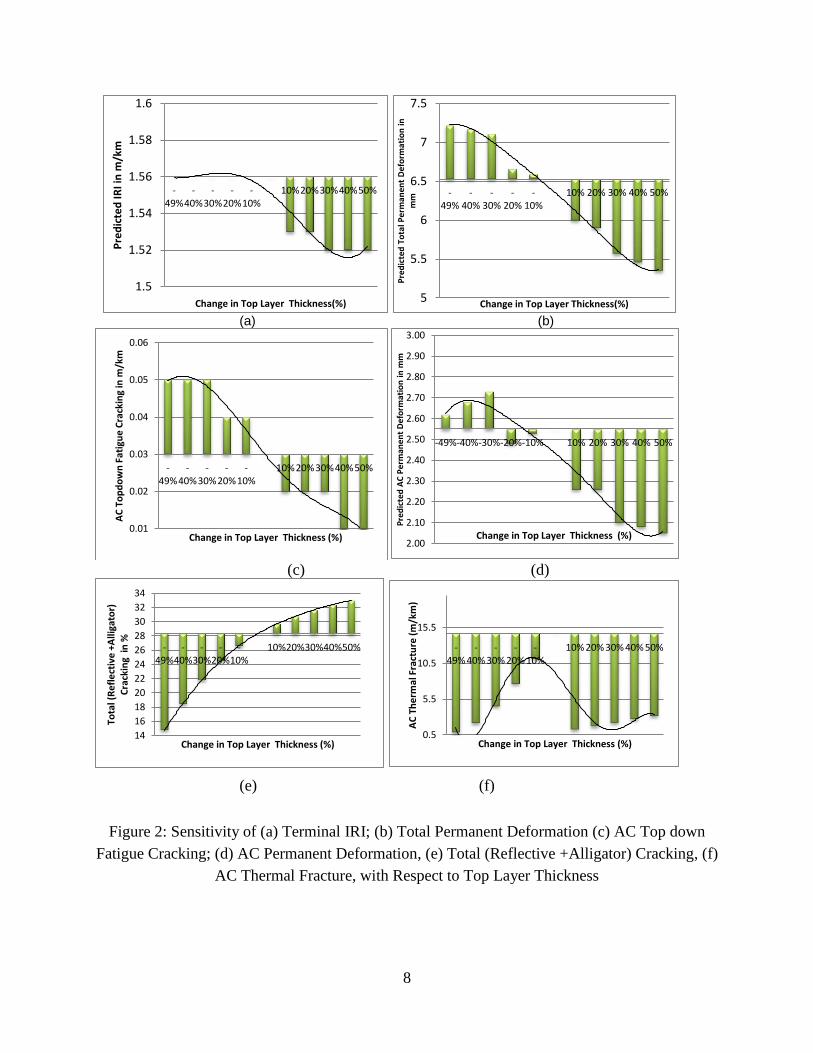
in output distresses are plotted for 46 input parameters to compare to each other. For example,
Table 3 shows the changes in distresses due to change in AADTT, and Figure 2 shows the changes
in the major sensitive distresses for changes in AC top layer thickness. Finally, changes in all
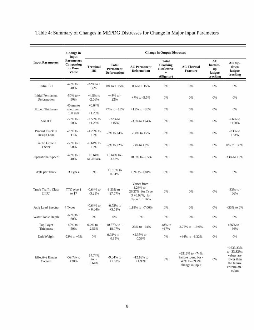
output distresses for change in input parameters are summarized in Table 4.
Table 2: MEPDG Outputs Distresses and Target Value of Failure in Ontario
Distress Type Target Value for
Freeway
Target Value for
Arterial
Terminal IRI (m/km) 1.9 2.3
Permanent Deformation - Total Pavement (mm) 19 19
Total Cracking (Reflective + Alligator) (percent) 100 100
AC Thermal Fracture (m/km) 190 190
AC Bottom-Up Fatigue Cracking (percent) 10 20
AC Top-Down Fatigue Cracking (m/km) 380 380
Permanent Deformation - AC only (mm) 6 6
After comparing the range of change in output distresses with respect to range of change in input
parameters, the input parameters that have individual substantial effects on distresses are screened
and listed in Table 5.
Finally, multiple linear regression analysis is carried out for each distress separately. In the
regression model only statistically significant effects (with the hypothesis of t statistics > 1.96) are
considered. The experimental design is rearranged with only the inputs that have significant
effects and multiple regression is carried out again for rearranged sample. In this way, significant
sensitive input parameters are found. The parameters are ranked based on the higher value of
coefficients. Finally, sensitive input parameters for each distress are summarized in Table 6.

7
Table 3: Changes in Distress for respective Change in AADTT
Change in
Input AADTT Change in Output Distresses
AADTT
changed
by %
Changed
AADTT
Termina
l IRI
(m/km)
Change
in
Termina
l IRI
(%)
Permane
nt
Deformat
ion -
Total
pavement
(mm)
Change in
Permanent
Deformation
Total (%)
Total
Cracking
(Reflective
+
Alligator)
(%)
AC
Thermal
Fracture
(m/km)
Change
in AC
Thermal
Fracture
(%)
AC
Bottom-
Up
Fatigue
Cracking
(%)
AC Top-
Down
Fatigue
Cracking
(m/km)
Change
in AC
Top-
Down
Fatigue
Cracking
(%)
Perma
nent
Defor
mation
- AC
only
(mm)
Change
in
Permane
nt
Deforma
tion -
AC only
(%)
-50% 703 1.52 -2.56% 5.12 -21.59% 28.32 14.64 0.00% 0 0.01 -66.67% 1.75 -
31.37%
-40.% 844 1.53 -1.92% 5.46 -16.39% 28.32 14.64 0.00% 0 0.02 -33.33% 1.93 -
24.31%
-30% 984 1.54 -1.28% 5.76 -11.79% 28.32 14.64 0.00% 0 0.02 -33.33% 2.10 -
17.65%
-20% 1125 1.54 -1.28% 6.04 -7.50% 28.32 14.64 0.00% 0 0.02 -33.33% 2.26 -
11.37%
-10% 1265 1.55 -0.64% 6.29 -3.68% 28.32 14.64 0.00% 0 0.03 0.00% 2.41 -5.49%
Base 1406 1.56 0.00% 6.53 0.00% 28.32 14.64 0.00% 0 0.03 0.00% 2.55 0.00%
10.00% 1547 1.56 0.00% 6.76 3.52% 28.32 14.64 0.00% 0 0.04 33.33% 2.68 5.10%
20.00% 1687 1.57 0.64% 6.97 6.74% 28.32 14.64 0.00% 0 0.04 33.33% 2.81 10.20%
30.00% 1828 1.57 0.64% 7.17 9.80% 28.32 14.64 0.00% 0 0.05 66.67% 2.93 14.90%
40.00% 1968 1.58 1.28% 7.35 12.56% 28.32 14.64 0.00% 0 0.06 100.00% 3.05 19.61%
50.00% 2109 1.58 1.28% 7.53 15.31% 28.32 14.64 0.00% 0 0.06 100.00% 3.16 23.92%
8
(a) (b)
(c) (d)
(e) (f)
Figure 2: Sensitivity of (a) Terminal IRI; (b) Total Permanent Deformation (c) AC Top down
Fatigue Cracking; (d) AC Permanent Deformation, (e) Total (Reflective +Alligator) Cracking, (f)
AC Thermal Fracture, with Respect to Top Layer Thickness
1.5
1.52
1.54
1.56
1.58
1.6
-49%
-40%
-30%
-20%
-10%
10%20%30%40%50%
Pre
dic
ted
IRI i
n m
/km
Change in Top Layer Thickness(%) 5
5.5
6
6.5
7
7.5
-49%
-40%
-30%
-20%
-10%
10% 20% 30% 40% 50%
Pre
dic
ted
To
tal P
erm
anen
t D
efo
rmat
ion
in
mm
Change in Top Layer Thickness(%)
0.01
0.02
0.03
0.04
0.05
0.06
-49%
-40%
-30%
-20%
-10%
10%20%30%40%50%
AC
To
pd
ow
n F
atig
ue
Cra
ckin
g in
m/k
m
Change in Top Layer Thickness (%)2.00
2.10
2.20
2.30
2.40
2.50
2.60
2.70
2.80
2.90
3.00
-49%-40%-30%-20%-10% 10% 20% 30% 40% 50%
Pre
dic
ted
AC
Pe
rman
ent
Def
orm
atio
n i
n m
m
Change in Top Layer Thickness (%)
14
16
18
20
22
24
26
28
30
32
34
-49%
-40%
-30%
-20%
-10%
10%20%30%40%50%
Tota
l (R
efl
ect
ive
+A
lliga
tor)
C
rack
ing
in %
Change in Top Layer Thickness (%)0.5
5.5
10.5
15.5
-49%
-40%
-30%
-20%
-10%
10%20%30%40%50%
AC
Th
erm
al F
ract
ure
(m
/km
)
Change in Top Layer Thickness (%)
9
Table 4: Summary of Changes in MEPDG Distresses for Change in Major Input Parameters
Input Parameters
Change in
Input
Parameters
Comparing
to Base
Value
Change in Output Distresses
Terminal
IRI
Total
Permanent
Deformation
AC Permanent
Deformation
Total
Cracking
(Reflective
+
Alligator)
AC Thermal
Fracture
AC
bottom-
up
fatigue
cracking
AC top-
down
fatigue
cracking
Initial IRI -40% to +
40%
-32% to +
32% 0% to + 15% 0% to + 15% 0% 0% 0% 0%
Initial Permanent
Deformation
-50% to +
50%
+4.5% to
-2.56%
+48% to -
22% +7% to -5.5% 0% 0% 0% 0%
Milled Thickness
40 mm to
maximum 100 mm
+0.64%
to +1.28%
+7% to +15% +11% to +26% 0% 0% 0% 0%
AADTT -50% to +
50%
-2.56% to
+1.28%
-22% to
+15% -31% to +24% 0% 0% 0%
-66% to
+100%
Percent Truck in
Design Lane
-25% to +
11%
-1.28% to
+0% -9% to +4% -14% to +5% 0% 0% 0%
-33% to
+33%
Traffic Growth
Factor
-50% to +
50%
-0.64% to
+0% -2% to +2% -3% to +3% 0% 0% 0% 0% to +33%
Operational Speed -40% to +
40%
+0.64%
to -0.64%
+0.64% to -
3.83% +8.6% to -5.5% 0% 0% 0% 33% to +0%
Axle per Truck 3 Types 0% +0.15% to
0.31% +0% to -1.81% 0% 0% 0% 0%
Truck Traffic Class
(TTC)
TTC type 1
to 17
-0.64% to
-3.21%
-1.23% to -
27.57%
Varies from -
1.26% to -26.27%; for Type
3 +0.98%; for
Type 5 1.96%
0% 0% 0% -33% to -
66%
Axle Load Spectra 4 Types -0.64% to
+ 0.64%
-0.92% to
+5.51% 1.18% to -7.06% 0% 0% 0% +33% to 0%
Water Table Depth -60% to +
60% 0% 0% 0% 0% 0% 0% 0%
Top Layer
Thickness
-49% to +
50%
0.0% to -
2.56%
10.57% to -
18.07% -23% to -94%
-48% to
+17% 2.75% to -19.6% 0%
+66% to -
66%
Unit Weight -23% to +3% 0% 0.92% to -
0.15% +2.35% to -
0.39% 0% +44% to -6.32% 0% 0%
Effective Binder
Content
-59.7% to
+20%
14.74% to -
0.64%
-9.04% to
+1.53%
-12.16% to
+1.96% 0%
+2512% to -74%,
failure found for -
40% to -59.7% change in input
0%
+1633.33%
to -33.33%;
values are lower than
the failure
criteria 380 m/km

10
Input Parameters
Change in
Input
Parameters
Comparing
to Base
Value
Change in Output Distresses
Terminal
IRI
Total
Permanent
Deformation
AC Permanent
Deformation
Total
Cracking
(Reflective
+
Alligator)
AC Thermal
Fracture
AC
bottom-
up
fatigue
cracking
AC top-
down
fatigue
cracking
Air Voids -40% to
+60%
-0.64% to
+5.13%
-1.53% to
+3.68%
-2.35% to
+4.71% 0%
140% for -40%
change in input; varies -19.19% to
836.75%for -20%
to +60% of input change
0%
-66.67% to +666.67%;
the values
are lower than failure
criteria of 380m/km
Reference
Temperature
-30% to
+23% 0% 0% 0% 0% 0% 0% 0%
Thermal
Conductivity
-30% to
+120%
-0.64% to
0%
-2.30% to
+3.83% -3.92% to +7.06% 0%
-18.24% to
+18.78% 0%
0% to
+33.33%
Heat Capacity -40% to
+40%
+0.64%
to -0.64%
+1.53% to -
1.53% +3.53% to -3.53% 0%
+89.48% to -
48.77% 0% 0%
Asphalt Binder Penetration Grade
5 types
+8.33% to 0%
-7.50% to +10.41%
-12.16% to +18.04%
0% to +0.35%
+1495% to -
100%; Failure found for 40-50
and 60-70;
0% 0%
Base Layer Thickness
-40% to +40%
0% to -0.64%
4.29% to -1.07%
-4.71% to +1.57% 0% +17.96% to
+3.42% 0% 0%
Resilient Modulus
of Base Layer
-60% to
+60%
+0.64%
to -0.64%
+6.28% to -
3.52% -3.14% to +1.57% 0% 0% 0%
+33.33% to
0%
Resilient Modulus of Subgrade Soil
-40% to +40%
+2.56% to -1.28%
+29.86% to -12.40%
-2.35% to -1.18% 0% 0% 0% 0% to
+33.33%
Table 5: Summary of Sensitive Input Parameters as per Range of Change in Output Distresses
Output Distress Sensitive Input Parameters as per Change in Output Distresses
Terminal IRI
1. Initial IRI, 2. Initial Permanent Deformation, 3 Milled Thickness, 4.
Percent of Truck in Design Lane, 5. AADTT, 6. Traffic Growth Factor, 7.
Operational Speed, 8. Axle per Truck, 9. TTC, 10. Axle Load Spectra, 11.
AC Effective Binder Content, Air Voids, AC Top Layer Thickness
Total Permanent Deformation
1. Initial Permanent Deformation, 2. Subgrade Resilient Modulus, 3. TTC,
4. AADTT, 5. AC Top Layer Thickness, 6. Asphalt Binder Penetration
Grade, 7. Milled Thickness, Initial IRI, 8. Percent Truck in Design Lane,
9. % Effective Binder Content, 10. Resilient Modulus of Base Layer, 11.
Base Layer Thickness, 13. Operational Speed
AC Permanent Deformation
1. AC Top Layer Thickness, 2.AADTT, 3. TTC Class, 4. Percent Truck in
Design Lane, 5. Milled Thickness, 6. Initial IRI, 7. Effective Binder
Content, 8. Binder Penetration Grade, 9. Operational Speed, 10. Axle Load
Spectra, 11. AC Thermal Conductivity, 12. Initial Permanent Deformation,
13. Air Voids, 14. Base Layer Thickness, 15 AC Heat Capacity

11
Output Distress Sensitive Input Parameters as per Change in Output Distresses
Total Cracking (Reflective +
Alligator)
1. AC Top Layer Thickness, 2. Asphalt Binder Penetration Grade.
AC Thermal Fracture
1. Effective Binder Content, 2. AC Binder Penetration Grade, 3. AC Air
Voids, 4. AC Heat Capacity, 5. AC Unit wt, 6. AC Top Layer Thickness,
7. AC Thermal Conductivity, 8. Base Thickness
AC Top-Down Fatigue
Cracking
1. Effective Binder Content, 2.AC Air Voids, 3. AADTT, 4. TTC, AC Top
Layer Thickness; 5. Percent Truck in Design Lane, 6. Subgrade Resilient
Modulus, 7. AC Thermal Conductivity, Traffic Growth Factor, Axle Load
Spectra, and Resilient Modulus of Base Layer
Table 6: Input Parameters as per Sensitivity Ranking for MEPDG Distresses
Distress Input Parameter as per Sensitivity Ranking
Terminal IRI
1. Initial IRI, 2. AC Air Voids, 3. AC Binder Penetration Grade, 4. Milled
Thickness, 4. AC Top Layer Thickness, 5. Initial Permanent Deformation,
6. AC Effective Binder Content
Total Permanent Deformation
1. Initial Permanent Deformation, 2. Subgrade Resilient Modulus, 3.
AADTT, 4. AC Top Layer Thickness, 5. Percent Truck in Design Lane,
6.TTC, 7. Milled Thickness
AC Permanent Deformation
1. 1. Percent Truck in Design Lane, 2.AC Top Layer Thickness, 3. TTC, 4.
Milled Thickness, 5. Initial Permanent Deformation, 6. AC Binder
Penetration Grade
Total Cracking (Reflective +
Alligator) 1. AC Top Layer Thickness
AC Thermal Fracture 1. 1. Effective Binder Content, 2. AC Binder Penetration Grade, 3. AC Air
Voids
AC Top-Down Fatigue
Cracking
1.
2. 1. AC Effective Binder Content, 2. AC Air Voids, 3. AADTT, 4. AC Top
Layer Thickness
5. CONCLUSIONS
This study is mainly focused on the identification of individual effects of independent input
parameters on MEPDG distresses. The relative influence of input parameters are required to
identify the requirements of high level of accuracy of inputs for precise prediction and calibration
of MEPDG distresses.
For statistical validity of investigations, an orthogonal experimental design based approach is used.
Orthogonal design is considered as the results are used for estimating a multiple linear regression

12
model. Since Local sensitivity focuses on the local impact of the input factors on the performance
of output, this process is carried out by varying certain input keeping other input parameters
constant. Based on a wide range of changes in output distresses with respect to range of change in
input parameters, the input parameters with individual substantial effects on distresses are listed.
The relative influences of different input parameters are found from the normalized values of the
variables of the regression model of each MEPDG distress. To identify statistically significant
sensitive parameters, multiple linear regression analysis is carried out. Sensitive input parameters
are screened and ranked with the hypothesis of t statistics > 1.96; and the higher value of
coefficients respectively.
Finally, it is found that terminal IRI is sensitive to initial IRI, AC air voids, AC binder penetration
grade, and milled thickness. Total permanent deformation is sensitive to initial permanent
deformation, subgrade resilient modulus, AADTT, AC top layer thickness, percent truck in design
lane, TTC, and milled thickness. Permanent deformation in AC layer is sensitive to percent truck
in design lane, AC top layer thickness, TTC, milled thickness, initial permanent deformation, and
AC binder penetration grade. For total cracking (reflective + alligator), sensitivity of only AC top
layer thickness is proven to be statistically significant. Sensitivity of effective binder content, AC
binder penetration grade, and AC Air Voids are proven to be statistically significant for AC
Thermal Fracture. Similarly, AC Top-Down Fatigue Cracking is found to be significant sensitive
to AC effective binder content, AC air voids, AADTT, and AC top layer thickness. However, no
sensitive input parameters are found for AC Bottom-Up Fatigue Cracking for the experimental
sample. Therefore, further investigation is required for AC Bottom-Up Fatigue Cracking.
Based on these identified sensitive input parameters, the accuracy level of major inputs of specific
distress are to be improved for realistic prediction and precise local calibration of MEPDG
distresses. The flexibility ranges of input parameters can also be selected based on this sensitivity
analysis for economic pavement design and future research.
The effort for obtaining high accuracy level of only sensitive input parameters rather than all input
parameters will be more efficient and economical. Laboratory tests of pavement sections can be
carried out for the specific properties only. For example, only AC air voids, AC binder penetration
grade, top layer thickness and AC effective binder contents are to be investigated to get level 1
accuracy for precise prediction of terminal IRI. Similarly, subgrade resilient modulus are to be
investigated for prediction of permanent deformation. Vehicles’ surveys for specific AADT,
percent truck in design lane, TTC type are to be conducted for prediction of permanent
deformation. Since from the analysis specific sensitive input properties are found for respective
distresses, it will be more efficient to get higher accuracy level of these properties through
laboratory tests or investigations. Future pavement design will also be efficient and economic
based on the higher accuracy level of the specific inputs. The local calibration will be precise,
realistic and efficient. Therefore, future prediction of distresses will be improved which will ensure
efficient future pavement management systems.

13
REFERENCES
1. NCHRP,(2004). “Guide for Mechanistic-Empirical Design of New and Rehabilitated
Pavement Structures”, Final Document, 1-37A Report, National Cooperative Highway
Research Program, Transportation Research Board National Research Council.
2. AASHTO, (2008). “Mechanistic-Empirical Pavement Design Guide: A Manual of
Practice”, Washington DC: AASHTO
3. MTO, (2012). “Ontario’s Default Parameters for AASHTOWare Pavement M-E Design-
Interim Report”, Ministry of Transportation, Ontario.
4. AASHTO, (2010). “Guide for the Local Calibration of the Mechanical-Empirical
Pavement Design Guide”, Joint Technical Committee on Pavements, 2008/2009
5. NCHRP, (2013). “Sensitivity Evaluation of MEPDG Performance Prediction”, National
Cooperative Highway Research Program, Research Results Digest 372, Transportation
Research Board of National Academies.
6. NCHRP, (2011). “Sensitivity Evaluation of MEPDG Performance Prediction”, National
Cooperative Highway Research Program, Final Report, Project 1-47, Iowa State
University Ames, IA.
7. Retherford, J. Q., and McDonald, M., (2011). “Estimation and Validation of Gaussian
Process Surrogate Models for Sensitivity Analysis and Design Optimization Based on the
Mechanistic–Empirical Pavement Design Guide” Transportation Research Record:
Journal of the Transportation Research Board, 2226: 119–126
8. Graves, R. C., and Mahboub, K. C., (2011) “Pilot Study in Sampling-Based Sensitivity
Analysis of NCHRP Design Guide for Flexible Pavements”, Transportation Research
Record: Journal of the Transportation Research Board,No. 1947: 123–135
9. Orobio, A., and Zaniewski, J., P.,(2011). “Sampling-Based Sensitivity Analysis of the
Mechanistic–Empirical Pavement Design Guide Applied to Material Inputs”
Transportation Research Record: Journal of the Transportation Research Board, 2226:
85–93.
10. Moya, J. P.A, and Prozzi, J., (2011). “Development of Reliable Pavement Models”,
Report SWUTC/11/161025-1 Texas
11. TRC, (2011). “Sensitivity Analysis for Flexible Pavement Design with the Mechanistic
Pavement Design Guide”. Transportation Research Circular E-C155
12. Hajek, J. J., Billing, R. J. and Swan D. J., (2011) “Forecasting Traffic Loads for
Mechanistic–Empirical Pavement Design” Transportation Research Record: Journal of
the Transportation Research Board, No. 2256 :151–158

14
13. Amador -Jime´ nez, E., and Mrawira, D. (2011). “Capturing variability in pavement
performance models from sufficient time-series predictors: a case study of the New
Brunswick road network”, Can. J. Civ. Eng, Published by NRC Research Pres
14. Siraj, N., Mehta, Y.A., Muriel, K.M., Sauber, R.W., (2009). “Verification of mechanistic-
empirical pavement design guide for the state of New Jersey”, Department of Civil and
Environmental Engineering, Rowan University, Glassboro, NJ, USA; Taylor & Francis
Group.
15. Guclu, A., Ceylan, H., Gopalakrishnan, K.,and Kim, S., (2009). “Sensitivity Analysis of
Rigid Pavement Systems Using the Mechanistic-Empirical Design Guide Software”,
Journal of Transportation Engineering, Vol. 135, ASCE, ISSN 0733.
16. Hall, K. D. and Beam, S. (2005). “Estimating the Sensitivity of Design Input Variables
for Rigid Pavement Analysiswith a Mechanistic–Empirical Design Guide” Transportation
Research Record: Journal of the Transportation Research Board, No. 1919: 65–73.
17. TAC (2013), “Pavement Asset Design and Management Guide” Transportation
Association of Canada, 2013