AN EXPERIMENTAL AND MODELING STUDY OF THEPHOTOCHEMICAL OZONE REACTIVITY OF ACETONE

Final Report to

Chemical Manufacturers Association

Contract No. KET-ACE-CRC-2.0

by

William P. L. Carter,

Dongmin Luo, Irina L. Malkina and John A. Pirece

December 10, 1993

Statewide Air Pollution Research Center, andCollege of Engineering Center for Environmental Research and Technology

University of CaliforniaRiverside, California 92521

SUMMARY

A series of environmental chamber experiments and computer model simulations were carried out to assess

the tendency of acetone to promote ozone formation in photochemical smog. The experiments consisted

of NOx - air photolysis of acetone by itself, and determinations of the effect of adding acetone on ozone

formation in model photochemical smog systems. Indoor chambers using either fluorescent blacklight or

xenon arc light sources and an outdoor chamber utilizing sunlight were employed. Similar experiments

utilizing acetaldehyde were carried out for comparison and control purposes. The gas-phase photochemical

mechanism for the atmospheric reactions of acetone was updated and was evaluated by model simulations

of the results of these experiments. The mechanism was found to overpredict the effect of acetone on

ozone formation and radical levels in the indoor chamber experiments with the blacklight light source and

in some of the outdoor chamber runs, but fit the results of other outdoor chamber runs and the experiments

runs using the xenon arc light source reasonably well. An adjusted mechanism which gave better

agreement with the blacklight experiments and with some of the outdoor runs was developed.

The updated and adjusted acetone mechanisms were then used in model calculations to assess the effects

of acetone on ozone formation under atmospheric conditions. This was done by calculating its incremental

reactivity (defined as amount of additional ozone formed caused by adding acetone to the emissions,

divided by the amount added) in model scenarios representing ozone episodes in 39 urban areas around

the United States. The incremental reactivities of ethane and a mixture representing total emissions

reactive organic gases from all sources were also calculated for comparison. The results indicate that

acetone forms 10-15% as much ozone on a per mass basis as total ROG emissions, while ethane forms

6-20% as much ozone, depending on conditions. The implications of these results on the question of

whether acetone should be exempt from regulation as an ozone precursor are discussed.

ii

ACKNOWLEDGEMENTS AND DISCLAIMERS

The authors wish to acknowledge and thank our project officer, Dr. David Morgott of Eastman

Kodak Co. for many helpful discussions and his support of this work. We also acknowledge Mr. William

Long for valuable assistance in carrying out the experiments, Mr. Ken Sasaki for assistance in developing

the outdoor chamber light model, Mr. Dennis Fitz for assisting in the management of this program and

reviewing parts of this report, Ms. Kathalena Smihula, Mr. Armando Avallone, Mr. Patrick Sekera, and

Mr. Jeff Friend for assisting in carrying out the experiments, and to Dr. Joseph Norbeck, the director of

the College of Engineering, Center for Environmental Research and Technology, for supporting the student

assistants working on this program and for providing some of the equipment which was used.

The experiments with acetone were funded by the CMA in part through providing support to

Coordinating Research Council Project No. ME-9, and in part through Contract No. KET-ACE-CRC-2.0.

Some of the base case and control experiments used in the data analysis and modeling for this program

were obtained under funding from the California Air Resources Board Contract No. A032-0692 and

Coordinated Research Council Project No. ME-9. In addition, the xenon arc light source used in this

study was funded by the National Renewable Energy Laboratory through Contract No. XZ-2-12075-1, and

the modular building where most of the experiments were conducted were provided by the California

South Coast Air Quality Management District through Contract No. C91323. We wish to thank these

agencies for their support of our programs.

The opinions and conclusions in this report are entirely those of the primary author, Dr. William

P. L. Carter. Mention of trade names or commercial products do not constitute endorsement or

recommendation for use.

iii

EXECUTIVE SUMMARY

Background

Photochemical ozone formation is caused by the gas phase reactions of volatile organic compounds

(VOCs) with oxides of nitrogen (NOx) in the presence of sunlight. To reduce ground level ozone and

achieve air quality standards, emissions of both NOx and VOCs are subject to controls. However, VOCs

are not equal in the amount of ozone formation they cause. If a VOC can be shown to make a negligible

contribution to ozone formation when it is emitted into the atmosphere, the United States Environmental

Protection Agency (EPA) can exempt it from regulation as an ozone precursor. Although the EPA has

no formal policy as to what constitutes "negligible" reactivity, it has the informal policy of using the

reactivity of ethane as the standard because ethane is the most rapidly reacting of the compounds which

has already been exempted. Thus if a compound forms comparable or less ozone on a per gram emitted

basis than ethane it can be considered for exemption.

Acetone is an important solvent species which reacts sufficiently slowly that it might reasonably

be considered as a candidate for exemption. Its net atmospheric reaction rate, on a mass basis, has been

estimated to be slightly less than that of ethane. However, the rate at which a VOC reacts is not the only

factor which determine its effect on ozone. Unlike ethane, acetone undergoes photodecomposition in the

atmosphere to form radicals, and increasing radical levels tends to cause increased rates of ozone

formation from the other VOCs present. If this effect were sufficiently important, it would mean that

acetone would cause more ozone formation than ethane.

The most direct quantitative measure of the degree to which a VOC contributes to ozone formation

in a photochemical air pollution episode is its "incremental reactivity" for that episode. This is defined

as the amount of additional ozone formation resulting from the addition of a small amount of the VOC

to the emissions in the episode, divided by the amount of compound added. This measure of reactivity

takes into account all of the factors by which a VOC affects ozone formation, including the effect of the

environment where the VOC reacts. The latter is important because the amount of ozone formation caused

by the reactions of a VOC depends significantly on how much NOx is present.

We have previously investigated methods for ranking photochemical reactivities of various VOCs

by calculating incremental reactivities of different VOCs under varying NOx conditions in model scenarios

representing various urban areas in the United States. Depending on the NOx conditions used, acetone

was calculated to be of comparable or greater reactivity than ethane. However, the chemical mechanism

used for acetone in these calculations has not been adequately experimentally verified, and thus it would

iv

not be appropriate to use these previous results as a basis for deciding whether it is appropriate to exempt

acetone from regulation as an ozone precursor.

This report describes a study designed to provide experimental data necessary to test and improve

the reliability of the atmospheric chemical mechanism for acetone, and then use the experimentally-verified

mechanism to re-evaluate the atmospheric reactivity of acetone relative to those of ethane and other VOCs.

Experimental Approach

A number of different types of environmental chamber experiments were carried out to evaluate

various aspects of acetone’s atmospheric reaction mechanism. These are summarized below:

Acetone - NOx experimentsconsisted of irradiations where acetone was the only compound present

in sufficient quantities to form ozone. This provides the simplest and most direct test of acetone’s

mechanisms. For control purposes, similar experiments were carried out using acetaldehyde instead of

acetone.

Incremental Reactivity experimentsconsisted of irradiations, in the presence of NOx, of a reactive

organic gas (ROG) "surrogate" mixture designed to represent ROG pollutants in ambient air, alternating

(or simultaneously) with irradiations of the same mixture with varying amounts of acetone added. This

provides the most direct test of a mechanism’s ability to simulate acetone’s incremental reactivity. For

control purposes, similar experiments were carried out using acetaldehyde. In addition, relevant results

of incremental reactivity experiments with ethane, carried out in a previous study, are also summarized

in this report.

Experiments with varying light sourceswere carried out to test the mechanism for acetone under

varying lighting conditions. This is important because one of the main factors affecting acetone’s

reactivity is the fact that it undergoes photolysis. The light sources used were blacklights, xenon arc

lights, and (in outdoor chamber experiments) natural sunlight.

Direct acetone vs ethane comparison experimentsconsisted of irradiations of a ROG surrogate -

NOx mixture with added acetone simultaneously with irradiations of the same mixture with a comparable

amount of added ethane on the other side. Although such experiments do not necessarily indicate the

relative reactivity of acetone and ethane in the atmosphere (because incremental reactivities depend on

conditions, and conditions in the chamber are different than in the atmosphere), they were conducted to

provide a comparison with similar experiments carried out at the University of North Carolina.

v

Chemical Mechanism Development

As part of this work, we also re-examined the literature concerning the atmospheric reactions of

acetone. The mechanism for its reaction with OH radicals was modified to be consistent with recent

laboratory results. The experimental data from which acetone’s photolysis quantum yields were derived

were evaluated and modeled, and some corrections were made based on the results of this analysis. The

resulting updated mechanism predicted a slightly lower reactivity for acetone in the atmosphere than the

one used previously. This updated mechanism was then evaluated by conducting model simulations of

the experiments discussed above.

Experimental and Mechanism Evaluation Results

The updated mechanism was found to simulate reasonably well the results of the experiments

using the indoor chamber light source most closely resembling sunlight and the outdoor chamber runs that

were conducted during the summer. However, this mechanism consistently overpredicted the rate of ozone

formation in the blacklight chamber experiments and also overpredicted the ozone formation in the

wintertime acetone - NOx run in the outdoor chamber. It is unlikely that this is due to incorrect

characterization of the blacklight intensity or spectra, because the model provides good simulations of the

photochemical reactivity of acetaldehyde, a VOC that photolyzes in a similar wavelength region as

acetone. Thus, it appears likely that the problem is that the model incorrectly represents how the acetone

photolysis quantum yields depend on wavelength.

An adjusted version of the updated acetone mechanism was developed that was considerably more

successful in simulating the experiments conducted in this study. The adjustment involves assuming that

the quantum yields fall off with increasing wavelength much more rapidly than indicated in previous work,

but that the fall off begins at a slightly longer wavelength. Although this adjustment is not theoretically

unreasonable, there is no basis for it other than fitting these environmental chamber data, which are highly

complex chemical systems with a number of other potential sources of error. The possibility that the

problem may be due to an incorrect characterization of the effect of the mercury lines in the blacklight

light source cannot be entirely ruled out. Therefore, in the assessment of the reactivities of acetone in the

atmosphere, we have used both the unadjusted (or standard) and the adjusted acetone mechanism in the

model calculations.

Atmospheric Reactivity Calculations

The adjusted and unadjusted updated acetone mechanisms were then used in model calculation

to assess the effects of acetone on ozone formation under atmospheric conditions. The incremental

reactivity of acetone, ethane, and the base ROG mixture (the mixture representing the sum of all VOCs

emitted into the atmosphere) were calculated in model scenarios representing ozone episodes in 39 urban

areas throughout the United States. It was found that the adjustment to the acetone quantum yields to fit

our chamber data caused an approximately 13% reduction in its incremental reactivity calculated for these

vi

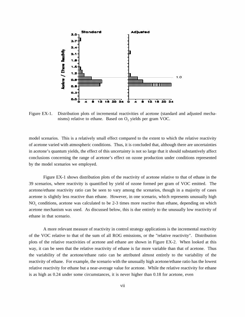
Figure EX-1. Distribution plots of incremental reactivities of acetone (standard and adjusted mecha-nisms) relative to ethane. Based on O3 yields per gram VOC.

model scenarios. This is a relatively small effect compared to the extent to which the relative reactivity

of acetone varied with atmospheric conditions. Thus, it is concluded that, although there are uncertainties

in acetone’s quantum yields, the effect of this uncertainty is not so large that it should substantively affect

conclusions concerning the range of acetone’s effect on ozone production under conditions represented

by the model scenarios we employed.

Figure EX-1 shows distribution plots of the reactivity of acetone relative to that of ethane in the

39 scenarios, where reactivity is quantified by yield of ozone formed per gram of VOC emitted. The

acetone/ethane reactivity ratio can be seen to vary among the scenarios, though in a majority of cases

acetone is slightly less reactive than ethane. However, in one scenario, which represents unusually high

NOx conditions, acetone was calculated to be 2-3 times more reactive than ethane, depending on which

acetone mechanism was used. As discussed below, this is due entirely to the unusually low reactivity of

ethane in that scenario.

A more relevant measure of reactivity in control strategy applications is the incremental reactivity

of the VOC relative to that of the sum of all ROG emissions, or the "relative reactivity". Distribution

plots of the relative reactivities of acetone and ethane are shown in Figure EX-2. When looked at this

way, it can be seen that the relative reactivity of ethane is far more variable than that of acetone. Thus

the variability of the acetone/ethane ratio can be attributed almost entirely to the variability of the

reactivity of ethane. For example, the scenario with the unusually high acetone/ethane ratio has the lowest

relative reactivity for ethane but a near-average value for acetone. While the relative reactivity for ethane

is as high as 0.24 under some circumstances, it is never higher than 0.18 for acetone, even

vii

Figure EX-2. Distribution plots of relative reactivities of acetone and ethane. Based on O3 yields pergram VOC.

using the more reactive standard mechanism for acetone. Conversely, while the relative reactivity for

ethane is as low as 0.05, it is never lower than 0.11 for acetone using the standard mechanism. Thus, the

relative reactivity range of acetone falls entirely within the range for ethane.

Conclusions

Although there are uncertainties in acetone’s atmospheric photooxidation mechanism, the

experiments and model simulations carried out in this work indicate that these uncertainties are not large

enough to substantially affect conclusions concerning acetone’s ozone formation potential relative to

ethane or other VOCs. The standard and the adjusted acetone mechanisms can be thought of as giving

respectively the upper and the lower estimates of acetone’s likely reactivity in any particular scenario.

The differences between these two estimates were small compared to the variability of acetone’s relative

reactivity from scenario to scenario.

The difference in acetone’s reactivity relative to ethane was also found to be less than the

variability of their relative reactivities from scenario to scenario. This variability is due more to the

variability of the reactivity of ethane with scenario conditions than that for acetone. On this basis, it can

be concluded the acetone and ethane can be considered to have essentially the same reactivity to within

their variability with environmental conditions.

We recommend, however, that a comparison of the reactivities of acetone and ethane not be used

as the sole basis for determining whether acetone should be exempt from regulation as an ozone precursor.

In considering whether a compound should be exempt, it is appropriate to assess its reactivity relative to

viii

the mixture of all VOC emissions. When EPA decided to exempt ethane, it effectively decided that it was

not necessary to regulate emissions of a VOC that could be almost 25% as reactive as the average of all

VOC emissions in terms of peak ozone concentrations, and almost 20% as reactive in terms of effect on

integrated ozone over the ambient ozone standard. When looked at this way, exempting a compound that

is calculated to be no more than 20% as reactive in terms of peak ozone, or 15% as reactive in terms of

integrated ozone over the standard, does not appear to be an inconsistent policy.

ix

TABLE OF CONTENTSPage

LIST OF TABLES . . . . . . . . . . . . . . . . . . . . . . . . . . . . . . . . . . . . . . . . . . . . . . . . . . . . . . . xii

LIST OF FIGURES. . . . . . . . . . . . . . . . . . . . . . . . . . . . . . . . . . . . . . . . . . . . . . . . . . . . . .xiii

INTRODUCTION . . . . . . . . . . . . . . . . . . . . . . . . . . . . . . . . . . . . . . . . . . . . . . . . . . . . . . . . . 1Background . . . . . . . . . . . . . . . . . . . . . . . . . . . . . . . . . . . . . . . . . . . . . . . . . . . . . . . . 1Approach. . . . . . . . . . . . . . . . . . . . . . . . . . . . . . . . . . . . . . . . . . . . . . . . . . . . . . . . . . 3

Acetone - NOx Experiments . . . . . . . . . . . . . . . . . . . . . . . . . . . . . . . . . . . . . . . 3Incremental Reactivity Experiments. . . . . . . . . . . . . . . . . . . . . . . . . . . . . . . . . . 4Acetaldehyde Experiments. . . . . . . . . . . . . . . . . . . . . . . . . . . . . . . . . . . . . . . . 6Acetone vsEthane Reactivity Comparisons. . . . . . . . . . . . . . . . . . . . . . . . . . . . 6Experiments with Varying Light Sources. . . . . . . . . . . . . . . . . . . . . . . . . . . . . . 7

EXPERIMENTAL METHODS . . . . . . . . . . . . . . . . . . . . . . . . . . . . . . . . . . . . . . . . . . . . . . . 10Environmental Chambers. . . . . . . . . . . . . . . . . . . . . . . . . . . . . . . . . . . . . . . . . . . . . . 10

ETC Blacklight Chamber. . . . . . . . . . . . . . . . . . . . . . . . . . . . . . . . . . . . . . . . 10DTC Blacklight Chamber (Dividable Teflon Chamber). . . . . . . . . . . . . . . . . . . 10Outdoor Teflon Chamber (OTC). . . . . . . . . . . . . . . . . . . . . . . . . . . . . . . . . . . 11Xenon Teflon Chamber (XTC). . . . . . . . . . . . . . . . . . . . . . . . . . . . . . . . . . . . 11

Experimental Procedures and Analytical Methods. . . . . . . . . . . . . . . . . . . . . . . . . . . . . 12Characterization Methods. . . . . . . . . . . . . . . . . . . . . . . . . . . . . . . . . . . . . . . . . . . . . 13

Temperature. . . . . . . . . . . . . . . . . . . . . . . . . . . . . . . . . . . . . . . . . . . . . . . . . 13Light Intensity and Spectra. . . . . . . . . . . . . . . . . . . . . . . . . . . . . . . . . . . . . . . 14Dilution . . . . . . . . . . . . . . . . . . . . . . . . . . . . . . . . . . . . . . . . . . . . . . . . . . . . 15Control Experiments. . . . . . . . . . . . . . . . . . . . . . . . . . . . . . . . . . . . . . . . . . . 15

Reactivity Data Analysis Methods. . . . . . . . . . . . . . . . . . . . . . . . . . . . . . . . . . . . . . . 15

MODEL SIMULATION METHODS . . . . . . . . . . . . . . . . . . . . . . . . . . . . . . . . . . . . . . . . . . . 17General Atmospheric Mechanism. . . . . . . . . . . . . . . . . . . . . . . . . . . . . . . . . . . . . . . . 17Acetone Mechanism. . . . . . . . . . . . . . . . . . . . . . . . . . . . . . . . . . . . . . . . . . . . . . . . . 19

OH Radical Reaction. . . . . . . . . . . . . . . . . . . . . . . . . . . . . . . . . . . . . . . . . . . 19Photolysis Reaction. . . . . . . . . . . . . . . . . . . . . . . . . . . . . . . . . . . . . . . . . . . . 20

Model Simulations of Chamber Experiments. . . . . . . . . . . . . . . . . . . . . . . . . . . . . . . . 22Light Characterization for Indoor Chamber Runs. . . . . . . . . . . . . . . . . . . . . . . 22Light Characterization for Outdoor Chamber Runs. . . . . . . . . . . . . . . . . . . . . . 23Temperature Characterization. . . . . . . . . . . . . . . . . . . . . . . . . . . . . . . . . . . . . 27Chamber Radical Source. . . . . . . . . . . . . . . . . . . . . . . . . . . . . . . . . . . . . . . . 27Other Chamber-Dependent Parameters. . . . . . . . . . . . . . . . . . . . . . . . . . . . . . . 28

Modeling Incremental Reactivity Measurements. . . . . . . . . . . . . . . . . . . . . . . . . . . . . . 29

x

EXPERIMENTAL AND MECHANISM EVALUATION RESULTS . . . . . . . . . . . . . . . . . . . . . 30Blacklight Chambers. . . . . . . . . . . . . . . . . . . . . . . . . . . . . . . . . . . . . . . . . . . . . . . . . 30

Acetone - NOx Experiments . . . . . . . . . . . . . . . . . . . . . . . . . . . . . . . . . . . . . . 30Acetone Reactivity Experiments. . . . . . . . . . . . . . . . . . . . . . . . . . . . . . . . . . . 30Acetaldehyde Experiments. . . . . . . . . . . . . . . . . . . . . . . . . . . . . . . . . . . . . . . 34Ethane Experiments. . . . . . . . . . . . . . . . . . . . . . . . . . . . . . . . . . . . . . . . . . . . 36

Xenon Chamber. . . . . . . . . . . . . . . . . . . . . . . . . . . . . . . . . . . . . . . . . . . . . . . . . . . . 38Acetone - NOx Experiments . . . . . . . . . . . . . . . . . . . . . . . . . . . . . . . . . . . . . . 38Acetaldehyde - NOx Experiments.. . . . . . . . . . . . . . . . . . . . . . . . . . . . . . . . . . 40

Outdoor Chamber. . . . . . . . . . . . . . . . . . . . . . . . . . . . . . . . . . . . . . . . . . . . . . . . . . . 40Acetone - NOx Experiments . . . . . . . . . . . . . . . . . . . . . . . . . . . . . . . . . . . . . . 40Acetaldehyde - NOx Experiments.. . . . . . . . . . . . . . . . . . . . . . . . . . . . . . . . . . 42Acetone Reactivity Experiments. . . . . . . . . . . . . . . . . . . . . . . . . . . . . . . . . . . 43Ethane vsAcetone Comparison Experiments. . . . . . . . . . . . . . . . . . . . . . . . . . 50

Model Simulations Using the Adjusted Acetone Mechanism. . . . . . . . . . . . . . . . . . . . . 52

ATMOSPHERIC REACTIVITY CALCULATIONS . . . . . . . . . . . . . . . . . . . . . . . . . . . . . . . . 56Scenarios Used for Reactivity Assessment. . . . . . . . . . . . . . . . . . . . . . . . . . . . . . . . . . 56

Base Case Scenarios. . . . . . . . . . . . . . . . . . . . . . . . . . . . . . . . . . . . . . . . . . . 57Maximum Incremental Reactivity (MIR) and Maximum Ozone Reactivity (MOR)

Scenarios . . . . . . . . . . . . . . . . . . . . . . . . . . . . . . . . . . . . . . . . . . . . . 59NOx Conditions in the Base Case Scenarios. . . . . . . . . . . . . . . . . . . . . . . . . . . 59

Incremental and Relative Reactivities. . . . . . . . . . . . . . . . . . . . . . . . . . . . . . . . . . . . . 59Reactivity Scales . . . . . . . . . . . . . . . . . . . . . . . . . . . . . . . . . . . . . . . . . . . . . . . . . . . 60Calculated Relative Reactivities of Acetone and Ethane. . . . . . . . . . . . . . . . . . . . . . . . 61

CONCLUSIONS . . . . . . . . . . . . . . . . . . . . . . . . . . . . . . . . . . . . . . . . . . . . . . . . . . . . . . . . . 68

REFERENCES . . . . . . . . . . . . . . . . . . . . . . . . . . . . . . . . . . . . . . . . . . . . . . . . . . . . . . . . . . 72

APPENDIX A. LISTING OF THE UPDATED SAPRC MECHANISM. . . . . . . . . . . . . . . . . . A-1

xi

LIST OF TABLESNumber page

1. Summary of conditions and selected results of the single compound - NOx - airexperiments. . . . . . . . . . . . . . . . . . . . . . . . . . . . . . . . . . . . . . . . . . . . . . . . . . . . . . . 31

2. Summary of conditions and results of the incremental reactivity and direct reactivitycomparison experiments.. . . . . . . . . . . . . . . . . . . . . . . . . . . . . . . . . . . . . . . . . . . . . . 32

3. Summary of conditions of base case scenarios used for atmospheric reactivity assess-ment. . . . . . . . . . . . . . . . . . . . . . . . . . . . . . . . . . . . . . . . . . . . . . . . . . . . . . . . . . . . 58

4. Comparison of incremental and relative reactivities in the MIR and MOIR scalescalculated using the updated and the SAPRC-90 mechanisms.. . . . . . . . . . . . . . . . . . . . 62

5. Relative ozone yield and IntO3>0.12 reactivities and reactivity ratios for acetone andethane in the base case scenarios and the MIR and MOIR scales.. . . . . . . . . . . . . . . . . 63

6. Summary of reactivities of acetone and ethane relative to the base ROG mixture.. . . . . . 71

A-1. List of model species used in the SAPRC-93 mechanism for the base case simulations. . A-1

A-2. Listing of SAPRC-93 mechanism as used to in the base case simulations.. . . . . . . . . . . A-4

A-3. Absorption cross sections and quantum yields for photolysis reactions.. . . . . . . . . . . . . A-9

xii

LIST OF FIGURESNumber page

1. Top Plot shows comparison of spectra of light sources used in the environmental chamberstudies. Bottom plot shows spectra of absorption cross sections x quantum yields forselected photoreactive species.. . . . . . . . . . . . . . . . . . . . . . . . . . . . . . . . . . . . . . . . . . . 9

2. Examples of fits of adjusted solar light model to light characterization data for twooutdoor chamber runs. Top plots: fits to direct and diffuse spectral data. Bottom plots:fits to changes with time in the data from the UV and broadband radiometers.. . . . . . . . 25

3. Experimental and calculated concentration-time profiles for selected species in the acetone- NOx runs carried out in the blacklight chambers.. . . . . . . . . . . . . . . . . . . . . . . . . . . . 35

4. Experimental and calculated concentration-time profiles for selected species in a selectedbase case run and in the added acetone reactivity experiments using the mini-surrogate inthe ETC blacklight chamber.. . . . . . . . . . . . . . . . . . . . . . . . . . . . . . . . . . . . . . . . . . . 36

5. Experimental and calculated concentration-time profiles for selected species in a selectedbase case run and in the added acetone reactivity experiments using the ethene surrogatein the ETC blacklight chamber.. . . . . . . . . . . . . . . . . . . . . . . . . . . . . . . . . . . . . . . . . 37

6. Experimental and calculated concentration-time profiles for selected species in a in theadded acetone reactivity experiments using the full surrogate in the DTC blacklightchamber. . . . . . . . . . . . . . . . . . . . . . . . . . . . . . . . . . . . . . . . . . . . . . . . . . . . . . . . . . 38

7. Experimental and calculated incremental reactivities, as a function of reaction time, in theadded acetone reactivity experiments using the mini-surrogate and the ethene surrogatein the ETC blacklight chamber.. . . . . . . . . . . . . . . . . . . . . . . . . . . . . . . . . . . . . . . . . 39

8. Experimental and calculated incremental reactivities, as a function of reaction time, in theadded acetone reactivity experiments using the full surrogate in the DTC blacklightchamber. . . . . . . . . . . . . . . . . . . . . . . . . . . . . . . . . . . . . . . . . . . . . . . . . . . . . . . . . . 40

9. Selected experimental and calculated results for the acetaldehyde - NOx experiments andthe added acetaldehyde reactivity experiments carried out using the blacklight cham-bers. . . . . . . . . . . . . . . . . . . . . . . . . . . . . . . . . . . . . . . . . . . . . . . . . . . . . . . . . . . . . 41

10. Experimental and calculated incremental reactivities, as a function of reaction time, in theadded ethane reactivity experiments. All experiments were carried out in the ETCblacklight chamber.. . . . . . . . . . . . . . . . . . . . . . . . . . . . . . . . . . . . . . . . . . . . . . . . . . 42

11. Experimental and calculated concentration-time profiles for selected species in the acetone- NOx runs carried out in the xenon arc chamber.. . . . . . . . . . . . . . . . . . . . . . . . . . . . . 43

xiii

Number page

12. Experimental and calculated concentration-time profiles for selected species in theacetaldehyde - NOx runs carried out in the xenon arc chamber.. . . . . . . . . . . . . . . . . . . 44

13. Experimental and calculated concentration-time profiles for selected species in the acetone- NOx runs carried out in the outdoor chamber.. . . . . . . . . . . . . . . . . . . . . . . . . . . . . . 45

14. Experimental and calculated concentration-time profiles for selected species in theacetaldehyde - NOx runs carried out in the outdoor chamber.. . . . . . . . . . . . . . . . . . . . . 46

15. Experimental and calculated concentration-time profiles for selected species in a in theadded acetone reactivity experiments using the full surrogate in the outdoor chamber. . . . 47

16. Experimental and calculated concentration-time profiles for selected species in a in theadded acetone reactivity experiments using the ethene surrogate in the outdoorchamber. . . . . . . . . . . . . . . . . . . . . . . . . . . . . . . . . . . . . . . . . . . . . . . . . . . . . . . . . . 48

17. Experimental and calculated incremental reactivities, as a function of reaction time, in theadded acetone reactivity experiments carried out in the outdoor chamber.. . . . . . . . . . . . 49

18. Experimental and calculated concentration-time profiles for ozone and NO, andexperimental temperature and UV light intensity data, in the acetone vsethane comparisonexperiments and the associated side equivalency test.. . . . . . . . . . . . . . . . . . . . . . . . . . 51

19. Top Plot shows comparison of spectra of light sources used in the environmental chamberstudies, for the wavelength range 300 - 320 nm. Bottom plot shows spectra of absorptioncross sections x quantum yields for the standard and the adjusted acetone mechanisms. . . 54

20. Distribution plots of ozone yield and IntO3>0.12 reactivities, relative to the base ROGmixture, for acetone and ethane in the base case scenarios.. . . . . . . . . . . . . . . . . . . . . . 64

21. Distribution plots of ratios of ozone yield and IntO3>0.12 reactivities of acetone relativeto ethane for the base case scenarios.. . . . . . . . . . . . . . . . . . . . . . . . . . . . . . . . . . . . . 65

22. Plots of ratios of ozone yield reactivities of acetone relative to ethane against theincremental reactivity of the base ROG for the base case scenarios. Reactivity ratios andranges of base ROG reactivities for the MIR and MOIR scales are also shown.. . . . . . . . 65

xiv

INTRODUCTION

BackgroundPhotochemical ozone formation is caused by the gas phase reactions of volatile organic compounds

(VOCs) with oxides of nitrogen (NOx) emitted into the atmosphere. To reduce ground level ozone and

achieve air quality standards, emissions of both NOx and VOCs are subject to controls. However, VOCs

are not equal in the amount of ozone formation they cause. If a VOC can be shown to make a negligible

contribution to ozone formation when it is emitted into the atmosphere, the United States Environmental

Protection Agency (EPA) can exempt it from regulation as an ozone precursor. Although the EPA has

no formal policy as to what constitutes "negligible" reactivity, it has the informal policy of using the

reactivity of ethane as the standard because ethane is the most rapidly reacting of the compounds which

has already been exempted. Thus if a compound forms comparable or less ozone on a per gram emitted

basis than ethane it can be considered for exemption. The bases for the decisions to exempt ethane but

not compounds more reactive than it has not been made clear, and they are probably largely subjective.

However, the existing precedent provides a guideline for evaluating possible exemption of additional

compounds which is relatively straightforward as long as the candidate compound is not of comparable

reactivity as ethane.

Acetone is an important solvent species which reacts fairly slowly in the atmosphere, and thus

might reasonably be considered as a candidate for exemption. Exempting acetone from regulation as an

ozone precursor would encourage its substitution for more reactive solvent species such as toluene, and

permit its use as a replacement for ozone depleters and greenhouse gases such as CFC-11, methyl

chloroform and methylene chloride (Eastman Chemical and Hoechst Celanese, 1993). Acetone is also an

example of a VOC which might be considered to have comparable reactivity as ethane. Meyrahn et al.

(1986) estimated the average annual atmospheric half life of acetone to be 22 days, which can be

compared to 25 days calculated for ethane for the same conditions. Acetone reacts with OH radicals

~15% slower than ethane (Atkinson, 1989), but unlike ethane it is also consumed by photolysis, resulting

in an overall half life which is essentially the same as that for ethane to within the uncertainties of the

estimates. However, acetone has a higher molecular weight than ethane, which means that fewer

molecules of acetone react per unit mass emitted. This makes acetone slightly less reactive than ethane

by this standard. Thus acetone would be a viable candidate for exemption by the ethane standard if the

only criterion used is the rate the compounds react in the atmosphere.

However, the rate at which a VOC reacts in the atmosphere is only one of several factors which

determines its effect on ozone formation (Carter and Atkinson, 1989; Carter, 1991, 1993a,b; Carter et al.,

1993a,b; Jeffries and Crouse, 1991). Other factors include the amount of ozone formed once a VOC

1

reacts, the effect of the VOC’s reactions on the reactions of other VOCs, and the effects of the reactions

of the VOC’s reaction products. (Carter and Atkinson, 1989; Carter et al., 1993a,b). For example, if a

VOC’s reactions (or those of its products) tend to promote radical levels in the atmosphere, then they

would increase the rates of reactions of all the VOCs present, and the rate of ozone formation from these

reactions. Because acetone photolysis is expected to form radicals (Atkinson, 1990; Meyrahn et al., 1986,

and references therein), acetone may have a greater effect on ozone than expected based on its reaction

rate alone.

The most direct quantitative measure of the degree to which a VOC contributes to ozone formation

in a photochemical air pollution episode is its "incremental reactivity" for that episode. This is defined

as the amount of additional ozone formation resulting from the addition of a small amount of the VOC

to the emissions in the episode, divided by the amount of compound added. This measure of reactivity

takes into account all of the factors by which a VOC affects ozone formation, including the effect of the

environment where the VOC reacts. The latter is important because the amount of ozone formation caused

by the reactions of a VOC depends significantly on how much NOx is present. If NOx is absent, no ozone

is formed and all VOCs have incremental reactivities of zero. Under low NOx conditions, ozone is NOx-

limited, and aspects of a VOCs mechanism affecting NOx removal rates are important in affecting

incremental reactivity. Under sufficiently high NOx conditions, ozone yields are determined by how

rapidly ozone is formed, and therefore aspects of the mechanism affecting overall radical levels tend to

be highly important.

Methods for ranking photochemical reactivities of various VOCs have been investigated by

calculating incremental reactivities of different VOCs under varying NOx conditions in model scenarios

representing 39 different urban ozone non-attainment areas in the United States (Carter, 1991; 1993a,b).

Several different incremental reactivity scales were developed, based on different NOx conditions and

different methods for measuring O3 impacts. These include the Maximum Incremental Reactivity (MIR)

scale, which reflects effects of VOCs on ozone yields under relatively high NOx conditions where VOCs

have their greatest effect on ozone, and the Maximum Ozone Incremental Reactivity (MOIR) scale, which

reflects effects of VOCs on ozone yields under the somewhat lower NOx conditions which are optimum

for formation of peak ozone concentrations. In addition, various "base case" reactivity scales were

developed to reflect (using various averaging or weighting methods) the distribution of incremental

reactivities under the varying NOx conditions associated with the different urban areas. These tended to

give similar rankings as the MIR or MOIR scales, depending on the derivation or ozone quantification

method used (Carter, 1991; 1993a,b).

The incremental reactivity of acetone (in terms of ozone per gram) was previously calculated to

be slightly less than that of ethane in the MOIR scale, but was 2-3 times greater than that of ethane in the

MIR scale. Thus the calculations indicate that the reactivity of acetone relative to ethane depends on NOx

2

conditions (Carter, 1993a,b). However, this factor of 2-3 maximum difference in reactivity is not large

considering that some VOCs are calculated to have MIR reactivities greater than 40 times that of ethane,

and that the calculated emissions-weighted average MIR reactivity of all VOCs is ~12 times that of ethane

on a per gram basis (Carter, 1993a,b).

It is important to recognize that these reactivity calculations for acetone were based on a chemical

mechanism for acetone which had not been experimentally verified. The chemical mechanism used to

calculate the MIR amd MOIR scales (Carter, 1990) was tested using a variety of smog chamber

experiments (Carter and Lurmann, 1991), but only one poorly-characterized outdoor chamber run was

relevant for testing the mechanism for acetone, and the mechanism significantly overpredicted the amount

of ozone which was formed. No reasonable adjustment of the acetone mechanism within its uncertainty

range would permit that acetone experiment to be adequately simulated (unpublished results from this

laboratory). Thus the predictions of this mechanism was not consistent with the limited data which was

available.

To provide data needed to improve the reliability of assessments of the reactivity of acetone with

respect to ozone, the Chemical Manufacturers Association (CMA) contracted us to carry out environmental

chamber experiments to measure the incremental reactivity of acetone, to provide data needed to test and

improve the reliability of the gas-phase atmospheric chemical mechanism for acetone. A second objective

was then to use the experimentally verified mechanism to assess the incremental reactivity of acetone

under atmospheric conditions, and in particular its incremental reactivity relative to that of ethane. The

results of this study is documented in this report.

ApproachThree types of environmental chamber experiments with acetone were conducted for this study.

These are acetone - NOx experiments, acetone incremental reactivity experiments, and direct acetone vs

ethane comparison runs. For comparison and control purposes, we also carried out acetaldehyde - NOx

experiments and incremental reactivity experiments for acetaldehyde, and include in our analysis results

of incremental reactivity experiments for ethane which were carried out previously (Carter et al., 1993a).

The utility of each are briefly described below.

Acetone - NOx Experiments

Acetone - NOx experiments consist of irradiations where acetone is the only reactive

organic present in sufficient quantities to significantly affect ozone. In most experiments, low levels (less

than ~10 ppb) of tracer species — usually cyclohexane or n-octane — are also present to monitor OH

radical levels from their relative rates of decay. These experiments test the acetone mechanism in the

absence of complications due to uncertainties in mechanisms for the other VOCs. However, it is not a

realistic representation of the chemical environment when acetone reacts in typical ambient atmospheres.

3

Such experiments do not test the ability of the mechanism to predict the effects of acetone on ozone

formation caused by the reactions of the other VOCs present in the atmosphere.

Incremental Reactivity Experiments

Incremental reactivity experiments consist of irradiations of a reactive organic gas (ROG)

"surrogate" - NOx air mixture, alternating (or simultaneously) with irradiations of the same mixture with

varying amounts of a test compound such as acetone added. The ROG surrogate - NOx mixture is

designed to approximate the chemical environment in polluted ambient atmospheres, and the irradiation

of this mixture without the added test compound is referred to as the "base case" experiment. The

experiment where acetone or some other test VOC is added is referred to as the "test" run. The difference

between ozone formation and NO oxidation in the test run relative to that in the base case run, divided

by the amount of test compound added, is the experimental incremental reactivity. Note that

"experimental" incremental reactivity refers to the effect of adding a finite amount of VOC, while

incremental reactivity in airshed model calculations refers to the effect of the VOC at the limit as the

amount added approaches zero (Carter and Atkinson, 1989). In addition, it should be emphasized that

since incremental reactivities are dependent on environmental conditions, and since it is not practical to

duplicate in the chamber all the environmental factors which might affect magnitudes of incremental

reactivities, incremental reactivities measured in chamber experiments should not be assumed to be

quantitatively the same as incremental reactivities in the atmosphere (Carter and Atkinson, 1989). The

latter can only be estimated using computer airshed model calculations. The utility of incremental

reactivity experiments is that they provide the most direct available means to test of the mechanism’s

ability to predict incremental reactivities in such calculations.

The "ROG surrogate" is the mixture of reactive organic compounds (ROGs) designed to represent

the more complex mixture of ROGs which are present in polluted atmospheres. Three types of ROG

surrogates were used in this study: the "mini-surrogate", the "lumped molecule" or "full" surrogate, and

the "ethene surrogate". Each have their own sets of advantages and disadvantages, as discussed below.

The Mini-Surrogateis a 3-component mixture consisting of 35% (as carbon) ethene, 50%

n-hexane, and 15% m-xylene. This was designed to be an experimentally simple representative of the

reactive organic compounds emitted into the atmosphere. Although this mini-surrogate is a significant

oversimplification of the complex mixture of ROGs present in the atmosphere (see, for example, Jeffries

et al. 1989a), model calculations show that use of this simpler mixture provides a more sensitive measure

of reactivities than use of more complex mixtures. In addition to having experimental simplicity while

representing the three major classes of emitted hydrocarbons, this surrogate has the advantage of having

a large data base of reactivity experiments for other VOCs using this surrogate (see Carter et al, 1993a).

4

The Full Surrogateis an 8-component mixture which is designed to represent the ROGs present

in the atmosphere in as much chemical detail they are represented in the airshed model simulations of their

reactions in the atmosphere. Airshed models which represent chemistry at the molecular level [i.e., models

other than those using the Carbon Bond mechanisms (Gery et al. 1988)] generally use the following

groupings of model species to represent ROG emissions: (1) less reactive alkanes such as n-butane; (2)

more reactive alkanes such as n-octane; (3) ethene; (4) terminal alkenes such as propene; (5) internal

alkenes such as the 2-butenes; (6) less reactive aromatics such as toluene; (7) more reactive aromatics such

as xylenes; (8) formaldehyde; (9) higher aldehydes such as acetaldehyde; and (10) ketones such as

methylethyl ketone. Except as indicated below, this surrogate uses a single "real" compound to represent

each of these model species. The selected representative compound for each group is generally the one

whose mechanism is used to represent that group because it dominates the group or because it is the

compound for which there is the most environmental chamber data available to test its mechanism.

Based on the amounts of model species which would be used to represent ambient base ROG

mixture utilized to calculate the MIR reactivity scale for the CARB (CARB, 1991; Carter, 1993a,b), the

target composition for the full surrogate (as carbon fractions) is: n-butane, 28%; n-octane, 18%; ethene,

27%; propene, 3%; trans-2-butene, 4%; toluene, 9%; m-xylene, 13%; formaldehyde, 1.6%; and 20% inert

carbon. (The "inert carbon" is not actually added, but is used when computing the equivalent amount of

ambient mixture the surrogate represents.) A separate species is not used for ketones because of their

relatively small contribution to the total reactivity of the mixture, and formaldehyde is used to represent

all aldehydes in the mixture (on a molar basis) because this substitution simplified the experiments and

was calculated not to have a measurable effect on the incremental reactivity results. Thus the 0.8%

formaldehyde + 1.5% acetaldehyde carbon is replaced by 1.6% formaldehyde. Model calculations indicate

that use of this surrogate in reactivity experiments would give indistinguishable results in reactivity

experiments as using full complex ambient mixtures (Carter, 1992). Thus this surrogate has the obvious

advantage of being the most realistic, while having the disadvantage of being the most complex to model.

The Ethene surrogateconsists of ethene alone. It is designed to be the simplest possible "ROG

surrogate" which can be used in reactivity calculations. A simple surrogate is advantageous because its

use should introduce the fewest uncertainties when evaluating the ability of a chemical mechanism to

predict experimental incremental reactivities. This is because errors in the model for the base ROG

surrogate can introduce extraneous or compensating errors in model simulations of experimental reactivity

measurements. To be suitable for this purpose, a compound or mixture (1) must have a reasonably well

characterized mechanism; (2) must react to form radicals which convert NO to NO2, (3) must provide

internal radical sources which are comparable in magnitude to those from complex mixtures; and (4)

should not be completely consumed before the experiment is completed. Ethene appears to be the best

candidate in this regard because it has a reasonably well characterized mechanism, has sufficient (but not

excessively high) internal radical sources, and because it reacts sufficiently slowly that it is not consumed

5

during an experiment. In addition, model calculations predict that using ethene as an ROG surrogate

would yield almost the same reactivities as using the 3-component mini-surrogate, except under highly

NOx-limited conditions (Carter, 1992).

The incremental reactivity experiments were carried out under NOx conditions similar to those

used to calculate the MIR scale. Thus they are referred to as "maximum reactivity" experiments. These

are NOx conditions where the VOCs have the greatest effect on ozone formation. In addition to providing

the most direct test of the ability of a model to predict maximum incremental reactivities, these

experiments provide a more sensitive test of the mechanism than experiments with lower NOx which are

less sensitive to the effects of the added VOC. In this study, the NOx levels employed were ~0.5 ppm.

The levels of the base ROG surrogate depended on the surrogate, but were such that ozone formation was

still occurring by the end experiments, indicating that NOx has not been completely consumed.

Acetaldehyde Experiments

For control and comparison purposes, the various types of experiments discussed above

were also carried out using acetaldehyde as the test compound. Acetaldehyde is a useful VOC for which

to compare the results with acetone because, like acetone, it is photoreactive and forms PAN as the major

product in both its OH radical and photolysis reactions (Atkinson, 1990, 1993). It can also be monitored

reliably and with reasonably good precision in our experiments. If the model performs as poorly in

simulating both acetone and acetaldehyde experiments, it may indicate that the problem is with the base

case model or the model for experimental conditions. If, on the other hand, the model performs well in

simulating results with one but not the other, it may indicate that problem is with the particular compound

which is poorly simulated.

Acetone vsEthane Reactivity Comparisons

Since one of the objectives of this study is to evaluate whether acetone or ethane forms

more ozone in the atmosphere, an obvious type of experiment is to determine the effects of equal amounts

of acetone and ethane on ozone formation under the same conditions. However, the effects of VOCs on

ozone formation are known to be highly dependent on the conditions in which they react (Dodge, 1984;

Carter and Atkinson, 1989; Carter, 1991, 1993a,b; Jeffries and Crouse, 1991). Because of this, if the

results of such experiments are to be used to make any conclusions concerning relative reactivities in the

atmosphere, the experiments need to duplicate, as closely as possible (and perhaps more closely than

practical) the conditions of the atmosphere. Even then, the results would be only applicable to the specific

sets of conditions being simulated.

The type of chamber experiment that would most closely duplicate atmospheric conditions would

be an incremental reactivity experiment in an outdoor chamber using a fully representative ROG surrogate.

Such an experiment was carried using the University of North Carolina dual outdoor chamber (Jeffries,

6

1993). In that experiment, a mixture consisting of a detailed surrogate + NOx + an amount of ethane equal

to the surrogate on a carbon basis was irradiated simultaneously with equal amounts (on a carbon basis)

of surrogate + NOx + acetone. The run was carried out under low ROG/NOx conditions. The result was

that there was no measurable difference in ozone formation on either side. This might be largely because

the amounts of ethane and acetone added were too small to cause a very large effect on the system in the

first place, so what was being measured is a difference between two small effects. This run illustrates the

small effects both of these compounds have on ozone, and the inconsequential effects of any differences

in their reactivities.

Because of the interest expressed by the EPA in this type of experiment (Dimitriades, 1993), we

decided to carry out a limited number of such experiments for this program. The main difference is that

the ethane and acetone were compared on an equal mass rather than an equal carbon basis, since VOCs

are regulated on the basis of mass. The amount of added ethane was such that it had an equal amount

of carbons as carbons being represented by the full surrogate (including inert carbons), and the amount

of added acetone was such that it had the same mass as the added ethane. Note that because of its greater

molecular weight per carbon, the amount of added acetone was 22% lower on a carbon basis than the

amount of added ethane.

Experiments with Varying Light Sources

One of the main factors affecting acetone’s reactivity is the fact that it undergoes

photolysis. Because of this, the nature of the light source used in the environmental chamber experiments

will be important. The approach used in this study was to conduct chamber experiments utilizing three

different light sources, each with their own unique advantages and disadvantages as discussed below. This

provides a much more comprehensive test for the atmospheric reaction mechanism for acetone, and

particularly the representation for its photolysis, than would be the case had only a single type of light

source been used.

The initial experiments for this study were carried out in chambers employing fluorescent

blacklights as the light source. Blacklights have the advantages of being a highly reproducible and easily

characterized light source which provides, at relatively low cost, the appropriate light intensity in the UV

region where most atmospheric species photolyze. Because of this, it has been utilized as the light source

for a large number of environmental chamber experiments which have been used for mechanism

evaluation (Carter and Lurmann, 1990, 1991, and references therein), including, most recently,

experimental measurements of maximum incremental reactivities of a wide variety of VOCs (Carter et al.,

1993a).

Figure 1 shows the solar and blacklight spectra in the wavelength region which affects most

photolysis rates in the atmosphere. The action spectra (absorption cross sections x quantum yields) for

7

NO2, acetone, and several other representative species are shown for comparison. The light source spectra

are all normalized to yield the same NO2 photolysis rate. While blacklights have the appropriate short

wavelength cutoff, it has higher intensity relative to sunlight in the ~330-360 nm region, and much lower

intensity at wavelengths greater than ~380 nm, where NO3 radicals andα-dicarbonyls photolyze. These

differences can be corrected for in model simulations of the experiments if the absorption cross sections

and quantum yields of the relevant photolyzable species are accurately known.

However, if there are uncertainties in the relevant absorption cross sections or quantum yields,

these will be corresponding uncertainties in the ability of the model to appropriately correct for these

differences. This is particularly important when evaluating mechanisms for photolyzable species such as

acetone. For this reason, several acetone - NOx, acetone reactivity, and acetaldehyde experiments were

carried out in an outdoor chamber using natural sunlight as the light source. Although the representative-

ness of the light source is obviously not a problem, the intensity and spectrum changes with time during

an experiment, making such experiments more difficult to characterize for quantitative mechanism

evaluation purposes. Time-varying temperature also makes such runs more difficult to characterize,

especially since some chamber effects are believed to be temperature dependent (Carter and Lurmann,

1990, 1991). Therefore, the evaluation of mechanisms using outdoor chamber data is more qualitative

than quantitative. However, if there are major errors in the representation of photolysis reactions in a

model which make its predictions grossly inapplicable to atmospheric lighting conditions, they should

become apparent when simulating such runs.

Another approach which can be used to evaluate mechanisms for photoreactive species is to

conduct indoor chamber experiments using a light source which is more representative of sunlight. This

could potentially provide the best features of both indoor and outdoor runs. The best commercially

available artificial light source we could find to approximate sunlight is xenon arc lights (Carter and

Walters, 1992). As shown on Figure 1, they provide a reasonably good (though not perfect) simulation

of sunlight throughout the entire wavelength region where most atmospheric species photolyze. For this

reason, we acquired, under DOE funding, a set of xenon arc lights, and constructed an environmental

chamber using them. Several acetone - NOx and acetaldehyde - NOx runs were conducted using this light

source.

8

Figure 1. Top Plot shows comparison of spectra of light sources used in the environmental chamberstudies. Bottom plot shows spectra of absorption cross sections x quantum yields forselected photoreactive species.

9

EXPERIMENTAL METHODS

Environmental ChambersAs discussed above, the experiments were carried out using four different environmental chambers

using three different types of light sources. These are described in this section.

ETC Blacklight Chamber

This chamber is the same as that utilized in the study documented by Carter et al. (1993a),

and is described in greater detail there. It consists of a single ~3000-liter, 2-mil thick FEP Teflon reaction

bag fitted inside an aluminum frame with banks of blacklights on the top and bottom, each bank consisting

of 30 Sylvania 40-W BL blacklamps. Reflective aluminum paneling is used on all sides. The temperature

is controlled by the laboratory air conditioning and fans which exchange the air around the reaction bag

with the air in the laboratory. Heaters are used prior to turning the lights on to minimize the temperature

rise which occurs when the lights are turned on. For runs prior to ETC-323, dry pure air for the

experiments was provided using the SAPRC air purification system which was described in detail

previously (Doyle et al., 1977). For subsequent runs, after the chamber was moved to a different location,

the dry pure air was supplied using an AADCO air purification system. This AADCO was also used to

supply the pure air for the other chambers described below.

DTC Blacklight Chamber (Dividable Teflon Chamber)

This chamber, which was newly constructed during the period of this study for use in

place of the ETC, is actually two adjacent chambers which can be operated simultaneously using the same

light source and temperature control system. These are referred to as the two "sides" of the chamber (Side

A and Side B) in the discussion of the results. The DTC consists of two 4600-liter 8’ x 6’ x 4’ 2-mil

thick FEP Teflon reaction bags in an 8’ x 8’ chamber enclosure room. The bags are interconnected with

two ports each with Teflon-coated fans and blowers which rapidly exchange their contents to assure that

reactants which are desired to have equal concentrations in each are equalized. The fans also mix the

contents within each chamber. The ports can then be closed to allow separate injections on each side, and

separate monitoring of each. The chamber enclosure room has two banks of blacklights on opposing

walls, with polished aluminum reflective material on the other walls and floor, and with perforated

aluminum reflective material on the ceiling, through which cooling air can be forced. Specially

constructed shaped aluminized plastic reflectors are used for the blacklights. The lighting system was

found to provide so much intensity that only half the lights were used in these runs. A thermostatted

temperature control system controlling a dedicated air conditioner for the chamber enclosure maintains the

temperature to within ±1˚ C and minimizes the sudden temperature rise which would otherwise occur

when the lights are turned on. The AADCO air purification system supplies pure dry air for this chamber.

10

This chamber would be expected to provide similar types of data as the ETC because it is

constructed of the same material, utilizes the same type of lights, and has approximately the same light

intensity. However, its dual chamber construction is particularly well suited for reactivity experiments,

with the base case irradiation being conducted simultaneously with the added test compound experiment

utilizing the same initial base case reactant concentrations and the same temperature profile and light

intensity. Alternatively, two different experiments can be conducted simultaneously.

Outdoor Teflon Chamber (OTC)

The SAPRC OTC, which has been described in detail elsewhere (Carter et al., 1984,

1986), consists of a ~30,000-50,000-liter, 2-mil thick FEP Teflon, pillow-shaped reaction bag located

outdoors. The reaction bag is supported by nylon ropes on a framework and held 2.5 feet off the ground

to allow air circulation under the chamber. A green indoor-outdoor carpet is located under the chamber.

When the chamber contents are not being irradiated, the reaction bag is covered by an opaque, grey trap

attached to a dual framework of steel tubing which can be readily opened to uncover the chamber and

initiate the irradiation. The AADCO air purification system supplies pure dry air for this chamber.

This chamber can be operated in a dual mode to allow two parallel experiments under the same

lighting and temperature conditions. This division of the chamber into two separate reactors, which can

be accomplished after reactants common to both chamber sides are injected and mixed, is accomplished

by means of three 1 1/4-in diameter cast-iron pipes, which are surrounded by foam to protect the Teflon

reactor. The reaction bag is divided by raising the lower pipe and placing it tightly between the upper

pipes, then rotating them by 180 degrees. Previous tests have shown that this forms a tight seal, with the

exchange between the chamber sides being less than 0.1% per hour (Carter et al., 1981). The chamber

is oriented such that the pipes dividing the chamber run in a north-south direction, with side A, by

convention, always being on the eastern half of the chamber. All OTC experiments discussed here were

conducted with the chamber in the divided mode.

Xenon Teflon Chamber (XTC)

This chamber, which was completed near the end of the time period of this study, is

similar in size and construction of one of the DTC chambers, but differs in the nature of the light source.

The XTC consists of a ~5200-liter, 6’ x 8’ x 4’ 2-mil thick FEP Teflon reaction bag located on one end

of a 8’ x 10’ chamber enclosure with reflective walls, floor and ceiling, and has a set of four Atlas

RM-65A 6.5 kw Xenon arc lights mounted on the opposite wall. The design objectives for this chamber

and lighting system is described elsewhere (Carter and Walters, 1992). It actually uses the same enclosure

as the DTC chambers, but in a different configuration. The side walls are the molded aluminized plastic

reflectors for the blacklights used for the DTC, with the blacklights removed. Sliding aluminum paneling

are used to prevent the Xenon lights from irradiating the chamber when they are being turned on and

stabilizing. AADCO air purification system supplies pure dry air for this chamber.

11

Experimental Procedures and Analytical MethodsThe chambers were flushed with dry purified air for 6-9 hours on the nights before the

experiments. The monitors were connected prior to reactant injection and the data system began logging

data from the continuous monitoring systems. The reactants were injected as described previously (Carter

et al, 1993a). For dual chamber (DTC or OTC) runs, the common reactants were injected in both sides

simultaneously (using a "T" in the injection line) and were well mixed before the chamber was divided.

In the case of the OTC, the reactants were mixed by manual agitation of the reaction bag, while with the

DTC the contents of side A were blown into side B and vise-versa using two separate blowers. Fans were

used to mix the reactants in the indoor chambers during the injection period, but these were turned off

prior to the irradiation. Dividing the OTC consisted of clamping the reaction bag in two using pipes,

while "dividing" the DTC consisted of closing the ports which connected the two reaction sides. After

the OTC or DTC were divided, the reactants for specific sides were injected and mixed. The irradiation

began by turning on the lights (for the blacklight chambers), opening the cover (for the OTC), or slighting

back the panels in front of the Xenon lights (which were turned on ~30 minutes previously). The

irradiation proceeded for 6 hours. After the run, the contents of the chamber(s) were emptied (by allowing

the bag to collapse) and flushed with purified air.

Ozone and nitrogen oxides were continuously monitored using commercially available continuous

analyzers with Teflon and borosilicate glass sample lines inserted directly into the chambers (ca 18 in.).

For DTC and OTC chamber runs, the sampling lines from each half of the chamber were connected to

solenoids which switched from side to side every 10 minutes, so the instruments alternately collected data

from each side. Ozone was monitored using a Dasibi Model 1003AH UV photometric ozone analyzer

and NO and total oxides of nitrogen (including HNO3 and organic nitrates) were monitored using either

a Columbia Model 1600 or a Teco Model 14B or 43 chemiluminescent NO/NOx monitor. The output of

these instruments, along with that from the temperature and (for OTC and XTC runs) light sensors were

attached to a computer data acquisition system, which recorded the data at periodical intervals, using 30

second averaging times. For single mode (ETC or XTC) chamber runs, the O3, NOx, and other continuous

data recorded every 15 minutes; for the divided chamber (DTC or OTC) runs, the data was collected every

10 minutes, yielding a sampling interval of 20 minutes for taking data from each side.

Organic reactants other than formaldehyde were measured by gas chromatography with FID

detection as described elsewhere (Carter et al., 1993a). GC samples were taken for analysis at intervals

from fifteen minutes to one hour using 100 ml gas-tight glass syringes. These samples were taken from

ports directly connected to the chamber. The syringes were flushed with the chamber contents several

times before taking the sample for analysis.

Formaldehyde was monitored using a diffusion scrubber system based on the design of Dasgupta

and co-workers (Dasgupta et al, 1988, 1990; Dong and Dasgupta, 1987), as described elsewhere (Carter

12

et al., 1993a). This system alternately collected data in sample (30 minutes), zero (15 minutes), and

calibrate mode (15 minutes), for a one hour cycle time. The readings at the end of the time period for

each mode, averaged for 30 seconds, were recorded on the computer data acquisition system, which

subsequently processed the data to apply the calibration and zero corrections. A separate sampling line

from the chamber was used for the formaldehyde analysis. For the DTC or OTC, a solenoid, which was

separate from the one used for O3 and NOx sampling, was used to select the chamber side from which the

formaldehyde sample was withdrawn, which alternated every 15 minutes. This yielded formaldehyde data

as frequently as every 15 minutes for single chamber (ETC and XTC) runs, and every 30 minutes for each

side of DTC and OTC runs.

Characterization MethodsTemperature

For the blacklight chambers, the temperature was monitored using an unshielded

thermocouple inside the chamber. Subsequent comparison of temperatures monitored with this method

with simultaneous readings using the aspirated temperature probe (discussed below) gave results which

were within ±0.2°C, indicating that heating of the thermocouple by the light from the blacklights is small.

This is expected because of the low visible and infrared energy of those lights. The temperature in the

ETC and DTC runs were typically 26-30˚C.

Prior to run XTC-090 the temperature was monitored in the XTC chamber using a thermocouple

inside the chamber shielded by a piece of reflective aluminum. During that period temperature probes

were also located in the formaldehyde and NOx/O3 sampling lines, but these data were not considered to

be as reliable because the sensors were outside the chamber. Although the temperature readings in the

sample lines were higher than the temperature in the laboratory, they tended to decrease with time during

the run, while the probes inside the chamber indicated that the temperature was increasing slightly.

Following run XTC-090, the temperature was monitored with the thermocouple inside an opaque 1/4" OD

sample line inside the chamber, with air being drawn through at a rate of 2 l/min. This is referred to as

the aspirated temperature probe. Provided that the flow rate past the sensor is sufficient, this method is

considered to give the more accurate temperature reading. Tests showed that a flow rate of be at least 2

l/min was required for the measured temperature to be independent of the flow. Comparison of the data

taken simultaneously indicated that the shielded probe in the chamber gave readings which were ~1.5˚C

higher than the aspirated shielded probe.

Except for run XTC-083, the temperatures monitored during XTC runs were highly consistent,

increasing rapidly from room temperature to 28-30° C immediately after the lights are turned on, to 29-31°

C by the end of the runs. For some reason, the temperature probe in the chamber gave readings which

were ~2 degrees higher for run XTC-083, though separate temperature probes in the sampling lines

indicated no differences between the temperature in that run and the others. For that reason, and the fact

13

that the temperatures were consistent from run to run for the other runs, we believe that the measured

readings were probably unreliable for that run.

An analogous change in temperature monitoring method was made for the outdoor chamber

experiments. For the runs in 1992 (run OTC-270 and earlier), temperature was monitored using unshielded

probes inside each chamber side, while for the other runs reported here (Runs OTC-271 and later)

temperature was monitored by shielded probes in the sample line, located slightly outside and underneath

the chamber.

Light Intensity and Spectra

The light intensity in the ETC and DTC was monitored by periodic NO2 actinometry

experiments utilizing the quartz tube method of Zafonte et al (1977), with the data analysis method

modified as discussed by Carter et al. (1993a). The measurements were made either with the quartz tube

in the reaction bag or with a Teflon film sleeve around the tube so the results would incorporate the effect

of the light passing through the chamber walls. Based on the results of these runs, the NO2 photolysis rate

associated with the blacklight chamber runs were as follows:

ETC-243 through ETC-247 and associated base case runs: 0.32 ± 0.02 min-1.

ETC-445: 0.336 ± 0.012 min-1.

All DTC runs: 0.38 ± 0.02 min-1.

The relative spectral distributions of the blacklight light sources were measured using a LiCor

LI-1800 portable spectrometer. The spectrum did not vary significantly with the chamber used or the age

of the lights, and the spectra taken using the LiCor using these chambers were essentially the same as

spectra of the lights in the SAPRC ITC chamber using a different spectrometer (Carter et al., 1984).

The light characterization for the XTC chamber was similar to that for the blacklight chambers,

with the absolute intensity being determined by NO2 actinometry using the quartz tube method, and the

relative spectra being determined by measurements using the Li-1800 spectrometer. However, the spectra

of xenon arc lights are expected to change gradually as the lights age, so spectra were taken 3-4 times

during each XTC run.

The NO2 photolysis rates measured by actinometry inside the XTC chamber was found to be 0.24-

0.26 min-1 after the lights were first installed (run XTC-79), and declined to a constant value of 0.23 min-1

in subsequent determinations (runs XTC-89 and XTC-100). The relative change in NO2 photolysis rate

with time during the experiments could also be obtained from the absolute light intensities measured by

the LiCor spectrometer. These data indicated that the NO2 photolysis rates declined by ~3% between runs

XTC-80 and around XTC-85, and was essentially constant after that. Based on the precision of the initial

actinometry results, the NO2 photolysis rates measured in the XTC are estimated to be uncertain by ~5%.

14

The sunlight intensity for the outdoor chamber runs was monitored continuously using an

Eppley UV radiometer and an Eppley PSP total broadband radiometer, and the global and diffuse light

spectra were measured approximately hourly during the runs using the LiCor spectrometer. The global

spectrum is that obtained with the unshaded instrument, while the diffuse spectrum is that obtained by

shading the sensor with a 10.0 cm disk held 90 cm from the sensor, positioned so that the shadow of the

disk covers the sensor (Jeffries, personal communication; Jeffries et al., 1989b). These data were used

as input to a light model, discussed later in this report, to calculate light intensity and spectra as a function

of time during the runs.

Dilution

Dilution due to sampling is expected to be small because the flexible reaction bags can

collapse as sample is withdrawn for analysis. However, some dilution occasionally occurs because of

small leaks, and several XTC runs had larger than usual dilution due to a larger leak which was

subsequently found and repaired. Information concerning dilution in an experiment can be obtained from

relative rates of decay of added VOCs which react with OH radicals with differing rate constants (Carter

et al., 1993a). All experiments had a more reactive compound (such as m-xylene or n-octane) present

either as a reactant or added in trace amounts to monitor OH radical levels. Trace amounts (~0.1 ppm)

of n-butane was added to experiments if needed to provide a less reactive compound for the purposes of

monitoring dilution. In many experiments, dilution rates were zero within the uncertainties of the

determinations.

Control Experiments

Several types of control experiments were conducted to characterize chamber conditions.

Ozone decay rate measurements were conducted with new reactors, and the results were generally

consistent with ozone decays observed in other Teflon bag reactors (Carter et. al. 1984, 1986). NOx-air

irradiations with trace amounts of propene or isobutene, or n-butane-NOx-air experiments, were conducted

to characterize the chamber radical source (Carter et al., 1982).

Reactivity Data Analysis MethodsAs described above, reactivity experiments consist of one or more "base case" run(s) combined

with a "test" experiment in which a VOC is added to the base case reactants. The results of these

experiments can be analyzed to yield several measures of VOC reactivity (Carter et al., 1993a,b), though

in this report we will focus on the effect of the VOC on the amount of NO reacted plus the amount of

ozone formed at hourly intervals in the experiment. This is abbreviated as d(O3-NO) in the subsequent

discussion. As discussed elsewhere (e.g., Johnson, 1983; Carter and Atkinson, 1987; Carter and Lurmann,

1990, 1991) this gives a direct measure of the amount of conversion of NO to NO2 by peroxy radicals

formed in the photooxidation reactions, which is the process that is directly responsible for ozone

15

formation in the atmosphere. The incremental reactivity of the test VOC relative to d(O3-NO) at time t,

designated IR[d(O3-NO)]tvoc, is given by

test based(O -NO) - d(O -NO)voc 3 t 3 tIR[d(O -NO)] =3 t [VOC] 0

where d(O3-NO)ttest is the d(O3-NO) measured at time t from the experiment where the test compound (e.g.,

acetone) was added, d(O3-NO)tbase is the corresponding value from the base case experiments where the

test VOC was not present, and [VOC]0 is the amount of test VOC added. The incremental reactivity with

respect to d(O3-NO) was calculated for each hour of the experiment.

The quantities d(O3-NO)test and [VOC]0 are obtained from the results of each of the individual test

experiments. The methods used to derive d(O3-NO)basedepended on whether the base case experiment was

being carried out at the same time under the same conditions in a divided or double chamber, as is the

case with DTC or OTC runs, or whether the base case experiment was carried out separately, as was the

case with the runs in the ETC. In the former case, the data from the base case side irradiated

simultaneously with the test run was used. In the ETC experiments, the effects of run-to-run variability

in temperature, light intensity, and initial reactant concentrations on d(O3-NO) had to be taken into

account. For these runs, the base case results used in the reactivity analysis of a particular test run were

derived from estimates, based on a linear regression analysis of results of many base case runs, of what

the result of a base case experiment would be if it were carried out with the same temperature, light

intensity, and initial base case reactant concentrations as the test run. The methods and data used in the

analysis of the ETC reactivity experiments are described in detail elsewhere (Carter et al., 1993a).

16

MODEL SIMULATION METHODS

Computer model simulations were conducted to evaluate the extent to which the results of these

experiments are consistent with predictions of a current chemical mechanism for the atmospheric reactions

of acetone and other VOCs. The mechanism was then used to simulate the incremental reactivities of

acetone, ethane, and other VOCs under atmospheric conditions. The following sections give descriptions

of the chemical mechanisms employed, of the methods used when simulating the chamber experiments,

and of the model and scenarios used when simulating atmospheric reactivities. The chemical mechanism

was updated for the purpose of this study. The overall mechanism used for all the atmospheric species

is described first, followed by a more detailed discussion of the mechanism used for acetone.

General Atmospheric MechanismThe chemical mechanism used as the starting point for this study is the "SAPRC-90" mechanism

as documented by Carter (1990), with updates for various VOCs made in conjunction with its use to

calculate the MIR scale for the California ARB (Carter, 1993a). This mechanism was then updated further

before use in this study, as discussed below. These updates take into account results of several recent

laboratory studies and incorporate some of the major recommendations made by Gery (1991) in his review

of the SAPRC-90 mechanism. The specific changes in the mechanism, relative to the SAPRC-90

mechanism used in the MIR calculation (Carter, 1993a,b), are as follows:

(1) The formaldehyde absorption cross-sections were updated based on the recent data of Cantrell

et al. (1990) and Rogers (1989). This results in a slight increase in the formaldehyde photolysis rate.

(2) The kinetics for the reactions of the acetyl peroxy radical with NO and NO2, which are

involved in the formation and decomposition of PAN, and the kinetics of the thermal decomposition of

PAN, were updated based on recent experimental results of Tuazon et al. (1991) and Bridier et al. (1991).

This causes the model to predict somewhat higher ozone formation rates than the SAPRC-90 mechanism.

(3) The SAPRC-90 mechanism uses model species whose photolysis rates are adjusted to fit

aromatic-NOx-air chamber experiments to represent the unknown photoreactive aromatic fragmentation

products (Carter, 1990). This approach is still used in the updated mechanism, except that the change in

the acetyl peroxy and PAN kinetics required reoptimization of these photolysis rates. In addition, the

action spectra (absorption coefficients x quantum yields) for these products were assumed to proportional

for the absorption cross section for acrolein (Gardner et al., 1987), rather than using the somewhat

arbitrary action spectrum in the SAPRC-90 mechanism. These changes were found not to significantly

17

affect the performance of the mechanism if the reoptimization is conducted using the same set of

experiments as used in the development of SAPRC-90.

(4) The mechanisms for the reactions of ozone with alkenes were modified to be consistent with

the data of Atkinson and Aschmann (1993), who observed much higher yields of OH radicals than

predicted by the SAPRC-90 mechanism. To account for these data, it was assumed that (1) the formation

of OH radicals dominates over other radical-forming fragmentation processes, and (2) in the reactions of

unsymmetrical alkenes, the more substituted Criegee biradical, which forms higher OH yields, are formed

in relatively higher yields than the less substituted biradicals. The modified ozone reactions for the

alkenes discussed in this paper are:

Ethene + O3 HCHO + (HCHO2)Propene + O3 0.6 HCHO + 0.4 CCHO + 0.4 (HCHO2) + 0.6 (CCHO2)trans -2-Butene + O3 CCHO + (CCHO2)Isobutene + O3 0.82 HCHO + 0.18 ACET + 0.18 (HCHO2) + 0.82 (C(C)CO2)

where CCHO and ACET represent acetaldehyde and acetone, and (HCHO2), etc., represent the excited

Criegee biradicals, which are represented as reacting as follows:

fast(HCHO2) 0.12 CO + 0.12 HO. + 0.12 HO2. + 0.88 (unreactive carbon)

fast(CCHO2) 0.3 HCHO + 0.3 CO + 0.6 HO. + 0.3 {CCO-O2.+ RCO3.} +0.3 {RO2-R.+ RO2.} + 0.9 (unreactive carbon)

fast(C(C)CO2) HCHO + HO. + {R2O2.+ RO2.} + {CCO-O2.+ RCO3.}

[See Carter (1990) for a description of the model species and the methods used to represent peroxy radical

reactions.] This is clearly an oversimplification of this complex system (e.g., see Atkinson, 1990, 1993),

but is intended to account for the observed OH radical yields and represent the major features affecting

these compounds’ reactivities. Note that this new mechanism gives substantially higher radical yields in

the ozone + alkene systems than the SAPRC-90 mechanism, particularly for internal alkenes.

(5) The reaction of NO with the peroxy radical formed in the reaction of OH radicals with

isobutene was assumed to form the corresponding hydroxyalkyl nitrate 10% of the time. This assumption

resulted in significant improvements to the fit of model simulations to ozone and PAN yields in isobutene

- NOx - air chamber experiments. Without this assumption, the model with the OH yields indicated by

the O3 + isobutene data of Atkinson and Aschmann (1993) significantly overpredicts O3 formation rates.

If lower radical yields in the O3 + isobutene reaction are assumed, the model significantly underpredicts

PAN (unpublished results from this laboratory).

18

(6) The representation of isooctane was modified to improve the model simulations of its

reactivity (Carter et al., 1993a,b).

(7) Several changes were made to the mechanism for acetone. These are discussed in the

following section.

A complete listing of this mechanism as used in the model simulations in this report is given in

Appendix A. Further updates to this mechanism are planned and it has not been as extensively evaluated

against the chamber data as the SAPRC-90 mechanism (Carter and Lurmann, 1991). However, it was

evaluated in model simulations of the results of the extensive set of maximum incremental reactivity

experiments recently completed in our laboratories (Carter et al, 1993a), and was found to perform

somewhat better than the SAPRC-90 mechanism in simulating these data.

Acetone MechanismAcetone is believed to react in the atmosphere primarily by photolysis and reaction with OH

radicals, and the available data concerning these reactions are discussed by Atkinson (1990, 1993).

Reaction with ozone would be expected to be of negligible importance (Atkinson and Carter, 1984), and

although there are no data available concerning its reaction with NO3 radicals, the rate constant would be

expected to be small (Atkinson, 1991). The mechanisms used in the model to represent the OH and

photolysis reactions are discussed below.

OH Radical Reaction

The representation of the OH + acetone used in the SAPRC-90 mechanism is based on

the recommendations of Atkinson (1990). The recommended rate constant expression is equivalent to k

= 1.92 x 10-13 (T/300)2 e0.11/RT cm3 molec-1 sec-1, which yields k = 2.31 x 10-13 cm3 molec-1 sec-1 at 300K.

The reaction is assumed to proceed as follows:

O O O OO NO" " 2 " "OH + CH CCH CH CCH CH CCH O CH CCH O3 3 3 2 3 2 2 3 2NO2

The alkoxy radical can either react with OH radicals, giving rise to methylglyoxal,

O OOO" 2 ""CH CCH O CH CCH + HO (a)3 2 3 2

or it undergo decomposition, giving rise to methylperoxy or acetylperoxy radicals, which react further to

ultimately form either formaldehyde + PAN or two formaldehyde + CO2, depending on the [NO]/[NO2]

ratio.

19

O O OO" " 2 "CH CCH O CH + CH C CH O + CH CO (b)3 2 3 3 3 2 3 2

At the time the SAPRC-90 mechanism was developed, there was no experimental information

available concerning the mechanism for this reaction, or the ka/kb branching ratio. This could be an

important factor affecting acetone’s reactivity because methylglyoxal is a highly photoreactive product

whose formation in the mechanism would enhance acetone predicted reactivity, while PAN formation is

a radical termination process whose formation would have an inhibiting effect. Based on an estimate

given by Atkinson (1990), the SAPRC-90 mechanism assumes that methylglyoxal formation occurs 80%

of the time, i.e., that ka/kb = 4.

However, more recent data and evaluations indicate that modifications to this OH + acetone

mechanism are appropriate. In an updated evaluation, Atkinson (1993) gives a slightly different

recommended rate constant expression for this reaction. The new recommendation is equivalent to k =

4.81 x 10-13 (T/300)2 e-0.457/RT cm3 molec-1 sec-1, which yields k = 2.23 x 10-13 cm3 molec-1 sec-1 at 300 K.

Although this gives essentially the same rate constants for the temperature range of these experiments, the

mechanism used in this study was updated to be consistent with this new recommendation.

More significantly in terms of predictions of acetone’s reactivity, recent data from Jenkin et al

(1993) indicate that reaction of the CH3COCH2O2 radical to form methylglyoxal is not important. This

is consistent with predictions of a revised estimation technique developed by Atkinson and Carter (1992)

based on recent data concerning decomposition and O2 reactions of analogous reactions of alkoxy radicals

formed from ethers and other compounds. Based on this, the updated OH + acetone mechanism used in

this study assumes that reaction (b) is the only significant process, and that methylglyoxal formation is

negligible. This results in a mechanism which predicts somewhat lower reactivity for acetone than does

SAPRC-90.

Photolysis Reaction

Available data concerning the photolysis of acetone under atmospheric conditions are

summarized in the latest IUPAC evaluation (Atkinson et al., 1992). The recommended absorption cross

sections and quantum yields are those of Meyrahn et al. (1986), while the SAPRC-90 mechanism (Carter,

1990) uses values from Calvert and Pitts (1966). The latter agree with the recommended values at

wavelengths greater than 310 nm, but are slightly lower at lower wavelengths, though the difference causes

only a ~1.5% change in the calculated atmospheric photolysis rate. Nevertheless, the updated mechanism

was modified to incorporate the recommended absorption cross sections.

20

The only energetically available photodecomposition reaction for acetone at wavelengths greater

than 300 nm is scission of the C-CO bond, forming, in the presence of oxygen, methylperoxy and acetyl-

peroxy radicals

O O OO" " 2 "CH CCH + hν CH C + CH CH CO + CH O3 3 3 3 3 2 3 2

In the presence of NO2 acetylperoxy radicals subsequently react to form PAN. There is disagreement in

the literature concerning the quantum yields for this reaction under atmospheric conditions. Gardner et

al. (1984) derived quantum yields of 0.07, approximately independent of wavelength over the 280-313 nm

region, based on acetone loss and yields of CO2, CO, CH3OH, and formaldehyde products when acetone

was photolyzed in air. Meyrahn et al. (1986) derived quantum yields which generally decreased

wavelength from 250-330 nm based on measuring yields of PAN in photolyses of ~150 ppm of acetone

and ~0.12 ppm of NO2 in air. The IUPAC panel recommends use of the data of Meyrahn et al (1986)

because they appeared to the evaluators to be more reasonable (Atkinson et al., 1992). These

recommended absorption cross sections were used in the SAPRC-90 mechanism.

The validity of the quantum yields reported by Meyrahn et al (1986) is based on the assumption

that under the conditions of their experiments all the acetyl peroxy radicals formed react to form PAN,

and that there is no other source of these radicals. However, as discussed in the previous section, the OH

reaction is also believed to form these radicals, and if sufficient OH were present in their experiments,

there could be an additional source of PAN from the this reaction and the reported quantum yields may

be high. To examine this, the conditions of these experiments were modeled using the updated SAPRC-90

mechanism. The model simulations predicted that the OH reaction was negligible in the experiments

carried out at wavelengths of 310 nm or less, but that this reaction forms ~10% of the PAN in the

experiments at 320 nm and ~50% of the PAN at 330 nm. This can be corrected for (albeit approximately)

by reducing the 320 nm quantum yields by 10% (from 0.028 to 0.026) and the 330 nm quantum yields

by a factor of ~2 (from 0.033 to 0.017). The corrections, particularly at 330 nm, must be considered to

be highly approximate because we probably did not simulate the conditions of the experiments exactly.

However, the factor of two correction of the 330 nm quantum yield gives a more reasonable decline in

quantum yields with wavelength than the uncorrected data, so the updated mechanism incorporated these

corrections to the Meyrahn et al. (1986) quantum yields. This correction causes a ~4% reduction of the

atmospheric photolysis rate for acetone.

The model simulations of the experiments at wavelengths of 310 nm or less predict that not all

the of the acetylperoxy radicals react to form PAN, since some will be lost by various peroxy + peroxy

radical reactions. The model simulations we conducted suggested that the PAN yields in those

experiments may underestimate the true quantum yields by ~15-20%. This would result in comparable

increases of the calculated atmospheric photolysis rates for acetone, since this wavelength region accounts

21

for most of the photolysis reaction. These estimates are uncertain because the predicted extent of peroxy

+ peroxy reaction is dependent on our model for the conditions of these experiments, whose accuracy is

unknown. The underprediction of quantum yields could be no more than ~20%, since otherwise the

corrected quantum yields for 250 - 260 nm would be greater than unity. For this reason, no such

correction to theλ < 210 nm quantum yields were applied. However, this analysis indicates that the

quantum yields which are up to ~20% higher than assumed in the model may not necessarily be

inconsistent with the data of Meyrahn et al (1986).

Because of the disagreement in the literature, the quantum yields for acetone photolysis must be

considered the most uncertain component of acetone’s atmospheric photooxidation mechanism. If the

quantum yields reported by Gardner et al. (1984) are assumed, the acetone photolysis rate is calculated

to be ~45% higher in the atmosphere and ~2 times higher in a blacklight chamber experiment, than

calculated using the corrected data of Meyrahn et al. (1986). Given the complexity of the chemical

systems utilized in both these studies, and the assumptions concerning the mechanisms that need to be

made in analyzing the results, the possibility that neither of these determinations are correct cannot be

ruled out.

Several adjustments were made to the assumed acetone quantum yields, and their wavelength

dependencies, to improve the fits of the model simulations to the experiments carried out in this study.

These are discussed in the Results section.

Model Simulations of Chamber ExperimentsThe testing of a chemical mechanism against environmental chamber results requires that the

model include appropriate representations for chamber-dependent effects such as wall reactions and

characteristics of the light source used during the experiments. The methods used to represent them in

this study are based on those discussed in detail by Carter and Lurmann (1991), adapted for these specific

sets of experiments as discussed by Carter et al. (1993a) or as indicated below. Where possible, the

parameters were derived based on analysis of results of characterization experiments carried out in

conjunction with these runs.

Light Characterization for Indoor Chamber Runs

Light characterization for indoor chamber runs consist of NO2 actinometry experiments

and measurements of the spectrum of the light source using the LI-1800 spectrometer. The former give

the absolute light intensities in terms of the NO2 photolysis rates, while the latter give information needed

to calculate the ratios of rates of all other photolysis reactions to that for NO2, given the absorption cross

sections and quantum yields for the NO2 and other photolysis reactions. In particular, the relative spectral

measurements are converted to absolute actinic fluxes by multiplying them by a factor which, when used

with the currently accepted NO2 absorption cross sections and quantum yields (Atkinson, 1990; Carter,

22

1990), result in the calculated NO2 photolysis rate being equal to the value derived from the actinometry

experiments. The absolute actinic fluxes are then used to calculate the rates of all the other photolysis

reactions in the model simulations.

This procedure uses the data from the actinometry experiments to give the absolute light

intensities, with the LI-1800 spectrometer only being used to obtain relative spectra. However, the

LI-1800 spectrometer is calibrated at the factory to give absolute light intensity readings, and thus, in

theory at least, it could be used to as a means to assess the accuracy of the actinometry experiments.

Unfortunately, the spectrometer measures light intensity on a plane, while photolysis rates are determined

by spherically integrated light intensities. To determine the latter from the former, and thus provide an

independent check of the accuracy of our actinometry measurements, we developed a model for the special

distribution of the light in the chamber, making measurements to estimate reflectances within the chamber

(unpublished results from this laboratory). The NO2 photolysis rate derived from this procedure was found

to be ~10% lower than that measured using the quartz tube actinometer. This is considered to be

agreement to within the uncertainties of the model and the measurements, and thus a validation of our NO2

actinometry method.

The spectra for the blacklight chambers were found to be essentially independent of chamber and

lamp age, at least in the wavelength region which affects photolysis rates. Thus the same spectrum was

used in the model simulations of these runs. However, the spectrum of the xenon arc light source used

in the XTC runs was found to change slowly with time, becoming somewhat weaker in the shortest

wavelengths as the lamps aged. The affected wavelengths were shorter than those which significantly

influence NO2 photolysis rates, and the intensity of the spectra indicated that NO2 photolysis rates

decreased by only ~3% during the course of this study. On the other hand, the photolysis of other species,

including acetone, are more affected by this change. For example, between runs XTC-80 and XTC-98

the photolysis rate of acetone, relative to that for NO2 was calculated to decline by ~14%. Because of

this, photolysis rates were calculated separately for each XTC run. Based on the results of the actinometry

experiments, combined with the monitoring of the light intensity with the spectrometer, we assign an NO2

photolysis rate of 0.24 min-1 for run XTC-80, 0.23 for run XTC-85 and those following, and intermediate

values for runs between XTC-80 and XTC-85. The photolysis rates for the other reactions were calculated

using the relative spectra measured during each individual run.

Light Characterization for Outdoor Chamber Runs

The light characterization data for the outdoor chamber runs consist of continuous UV and

broadband radiometer data, and approximately hourly global and diffuse solar spectra taken using the

LI-1800 spectrometer. The global and diffuse spectra, along with the JSPECTRA solar light model

developed by Jeffries (1988, 1989b, 1991), were used as the primary means for light characterization for

modeling purposes. The procedure employed is only applicable to clear sky conditions, so no runs on

23

cloudy or overcast days were used for mechanism evaluation. The radiometer data was used as a cross-

check to assure that the light conditions were not changing abruptly between the times spectral

measurements were made. The outdoor chamber light characterization procedures will be documented in

a subsequent report, and will only be summarized here.

The JSPECTRA solar light model is designed to calculate ground-level solar spectra given relevant

parameters such as time of day, day of year, total ozone column, atmospheric aerosol parameters, and

extraterrestrial solar fluxes. It can be used either to calculate spherically integrated actinic fluxes for

calculation of photolysis rates or to predict global or diffuse spectra as measured by the LiCor

spectrometer. Some of the inputs to the program, such as the time of day or day of year, are known,

others, such as the extraterrestrial fluxes, are assumed not to be variable and are provided with the

program, while other inputs, such as the ozone column and the aerosol parameters, are uncertain or

variable. The most sensitive of the uncertain inputs were adjusted, using a non-linear optimization

algorithm, to fit the global and diffuse LiCor spectra taken during the run, while for the less sensitive

parameters the defaults used by Jeffries (1988) for "summer conditions" were used in all calculations.

Although moderately good fits of adjusted model calculation to LiCor spectra could obtained by adjusting

only the parameters in the JSPECTRA model, for best fits to the data three separate parameters were

added to scale the overall intensity as a function of wavelength. These consisted of scaling factors for

the intensities at 300, 500, and 800 nm; the scaling factors for other wavelengths were obtained by linear

interpolation of these. With the set of parameters we used, these scaling factors were consistently 0.7, 1,

and 1.1 at these three wavelengths, respectively. An example showing the comparison obtained between

the adjusted model calculation and the global and diffuse LiCor spectra is shown on Figure 2

The results of the optimization of the JSPECTRA input parameters could then be used to calculate

spherically integrated actinic fluxes for the times the LiCor spectra were taken. The calculated spherically

integrated fluxes were not sensitive to the specific set of JSPECTRA parameters optimized, as long as the

model could closely simulate the direct and diffuse LiCor data. If the run was carried out on a clear day,

the parameters affecting light fluxes might reasonably be assumed not to change abruptly with time. In

this case, the values of the adjusted parameters for times between those where LiCor data were taken could

be estimated by linear interpolation of the optimized values. Based on this assumption, parameters were

estimated at each 20 minute interval during the run, from which actinic fluxes for those times were

calculated. The fact that this assumption is not valid for cloudy days is not a significant limitation because

the JSPECTRA model was not designed to calculate solar fluxes for those conditions in any case. For

this reason, only data from clear day runs were characterized for modeling purposes. The few runs carried

out on days with unfavorable weather are not discussed.

The JSPECTRA program, with its time-varying inputs derived as discussed above, could also be

used to calculate how the data from the UV and broadband radiometers should vary with time. Thus,

24

Figure 2. Examples of fits of adjusted solar light model to light characterization data for twooutdoor chamber runs. Top plots: fits to direct and diffuse spectral data. Bottom plots:fits to changes with time in the data from the UV and broadband radiometers.

25

while this method does not directly utilize these data in the photolysis rate calculations, they can be used

as a check on the appropriateness of the model’s interpolations. Typical results are included on Figure

2, which shows plots of observed and calculated radiometer data vs. time for run OTC-274. In general,

the model gave somewhat better predictions of the time profiles of the broadband data than the UV data.

This can be attributed to the fact that the spectral response of UV radiometers such as those employed in

this study are not particularly well characterized, and the JSPECTRA model uses a highly idealized

representation in this regard.

The above procedure predicts light spectra outside the chamber, but the relevant quantities are the

light spectra inside the Teflon reaction bag. Jeffries et al. (1989b) measured light reflection and

transmission through 2 mil and 5 mil FEP teflon film as a function of wavelength and the incidence angle

of the light beam, and developed a parameterized model to fit these data. Although this model includes

a term for absorption, the fraction of light absorbed is small (less than 1% for 2-mil film) and can be

neglected. Thus only loss due to reflection on the outer chamber walls, or enhancement due to reflection

on the inner walls, need be considered. The OTC can be thought of as a transparent bag suspended in

space, with light entering it from all directions. If the effect of the presence of the bag on the light

coming in from the bottom is neglected, it can be shown that the light enhancement by the reflections

from inside the bag just makes up for the light lost due to the reflection when it enters the bag, with the

result being that the intensity (and spectrum) inside the bag should be exactly the same as outside. The

principle behind this is exactly the same as the principle behind the arguments given by Zafonte et al.

(1977) when they concluded that reflections off quartz tubes do not affect results of actinometry

measurements using such tubes. Consistent with this is the fact that no significant differences were

observed when NO2 actinometry measurements were made inside and outside the OTC on the same days.

The assumption that the presence of the OTC does not affect light coming from the bottom is not

totally valid because the reaction bag is sufficiently close to the ground that all the light coming from the

bottom has first passed through the bag, and was thus attenuated by the first reflection from the top. An

approximate correction for this was made based on assuming the top and the bottom of the chamber are

flat planes of film parallel to the surface, and that the albedo of the carpet under the chamber is the same

as the general albedo which is the default in the JSPECTRA model. Parameterized fits to 2-mil FEP

Teflon transmission data provided by Jeffries (private communication) were used to calculate the

transmissions and reflectance through the chamber walls. This is a fairly small correction, causing the

predicted in-chamber photolysis rates to be ~4% than those calculated for outside.

The in-chamber actinic fluxes calculated for every 20 minutes during the run were used as input

into model when simulating the run. The model then calculated the photolysis rates for these periods

using the absorption cross sections and quantum yields for the various reactions. The photolysis rates

26

were updated at each time step in the simulation, with the model deriving the photolysis rates for

intermediate times between these 20 minute intervals by linear interpolation.

Temperature Characterization

The temperature was observed to varied with time in both the indoor and the outdoor

chamber runs, though the variation was much greater in the latter case. The measured temperature data

(with any applicable corrections, discussed below), were fit to various straight line segments, and these

lines were then used to describe how the temperature varied with time in the model simulations.

Subjective judgement was used in determining how many different line segments were required to fit the

time variation of the temperature data, but a least squares error optimization program was used to

determine the best fit lines once the end points of the line segments have been specified. A single line

was sufficient to describe variation in most of the indoor runs, but usually 3-4 lines were required for

outdoor runs. For divided chamber runs (OTC and DTC), separate temperature profiles were derived from

the data for each side.

The ETC and DTC temperature measurements made with the unshielded probes inside the chamber

were used without correction. The XTC temperature measurements made with the aspirated temperature

probe were assumed to be accurate and were used without correction. For runs where such data are not

available, data taken with the shielded thermocouple inside the chamber were used after being corrected

by subtracting 1.5 degrees, as indicated by comparison tests. As discussed above, the in-chamber

temperature data for run XTC-083 appear to be anomalous, and the temperature profiles derived for

modeling run XTC-086 were also used for modeling this run because the temperature readings in the

sampling line were very close for these two runs.

The OTC temperature measurements made with the thermocouple in the sampling line immediately

outside the chamber were assumed to be accurate and used without correction. This is applicable to all

runs discussed in this report except OTC-270, where unshielded probes inside the chamber were used.

There are no data concerning the temperature corrections appropriate for this run. There was also some

inconsistency between temperature measurements from the two sides of the chamber. Because of this, this

run was modeled with the temperature input varied within its probable uncertainty.

Chamber Radical Source

As discussed elsewhere (Carter et. al, 1982; Carter and Lurmann, 1990, 1991), model

simulations of chamber runs must include a representation for a chamber radical source. Although certain

runs, especially alkane - NOx - air runs, are highly sensitive to this parameter, it is less important in

affecting results of runs containing complex mixtures designed as atmospheric surrogates, or runs

containing species, such as acetone, which are radical initiators. Because of the high sensitivity of alkane

- NOx runs to the chamber radical source (Carter et al., 1979), we carried out n-butane - NOx - air

27

irradiations for determining this parameter. The radical source is then adjusted in model simulations to

fit the NO oxidation observed in these runs. We found that modeling n-butane runs is a more sensitive

method for determining the chamber radical source than analysis of radical tracer - NOx runs as we have

employed previously (Carter et al., 1982).

For the DTC and XTC runs, the chamber radical source parameters were adjusted to fit results of

n-butane - NOx irradiations carried out in those chambers. Based on these results, an OH radical input

rate used for both these chambers was 0.06 ppb x the NO2 photolysis rate. This is lower than the range

of values used for the SAPRC ITC (Carter and Lurmann, 1990, 1991), but within the range used for the

ETC runs (Carter et al., 1993a).

Since the chamber radical source is expected to be dependent on temperature (Carter et al., 1982),

and since temperature varies widely in outdoor runs, use of a temperature-dependent radical source

parameter would be appropriate when modeling such runs. Better results in modeling alkane - NOx runs

carried out in the UNC outdoor chamber was obtained when a temperature-dependent radical source was

assumed (Carter and Lurmann, 1990, 1991). The three n-butane - NOx runs carried out in the OTC for

this study had average temperatures of 309, 312, AND 317° K, and, if the radical source input parameter

(OH input rate / NO2 photolysis rate — given in units of ppb) is assumed to be independent of

temperature, the values which resulted in model simulations best fitting these runs were 0.2, 0.3, and 0.3-

0.4 ppb, respectively. All three runs could be fit by assuming the following temperature dependence for

the ratio of the OH input flux to the NO2 photolysis rate: 290°K: 0.02 ppb; 300°K: 0.05 ppb; 310°K: 0.3

ppb; and 320°K: 0.4 ppb. Values for intermediate temperatures were obtained by interpolation. The value

for 300° K is based on typical values for indoor runs, and the value for 290° K is an estimate.

Other Chamber-Dependent Parameters

The various other chamber dependent effects which are included in the model simulations

of these chamber runs include humidity, dilution, ozone decay rate, initial nitrous acid, NOx offgasing

rates, N2O5 hydrolysis, and NO conversion due to background VOCs (Carter and Lurmann, 1990, 1991;

Carter et al., 1993a). In the case of the indoor Teflon chambers (the ETC, DTC, and XTC), these were

represented in a similar manner as discussed by Carter et al. (1993a) for the ETC, except as follows. The

dilution rates were based on decay rates of slowly reacting species in the individual runs, when such data

were available. If not, the default dilutions used were those derived from the ETC data (Carter et al.,

1993a). No initial nitrous acid was assumed to be present because the NOx injection procedures employed

were designed to eliminate its formation (Carter et al., 1993a).

The chamber-dependent parameters for the OTC runs were the same as used in our previous

mechanism evaluation studies using data from this chamber (Carter and Lurmann, 1990, 1991), except that

28

dilution rates were based on decay rates of slowly reacting observed in individual runs were used when

such data were available.

Modeling Incremental Reactivity MeasurementsModeling of incremental reactivity measurements consisted of conducting model simulations of

both the base case and the added test VOC experiment, and then analyzing the results using the same

procedures as employed experimental data. In the case of the ETC runs, where there is no single base

case run associated with any particular test run, the base case simulation associated with a particular test

run consisted of modeling the conditions of the that test run, but without the test compound added.

As discussed by Carter et al. (1993a,b), the SAPRC-90 mechanism was found to underpredict the

rate of ozone formation in the base case mini-surrogate - NOx experiments used in conjunction with the

ETC acetone reactivity runs. The updates to the mechanism discussed above did not significantly change

this. If the model cannot adequately simulate the base case experiments, it cannot be used as a reliable

test of mechanisms for test compounds to predict their incremental reactivities in those experiments.

Therefore, in the model simulations of the mini-surrogate experiments only, the model for m-xylene in

the mini-surrogate was adjusted slightly so the model could better simulate the base case experiment

(Carter et al, 1993a,b). The modified m-xylene mechanism is included in the reaction listing in Appendix

A. Note that this adjustment was not used in the simulation of the full surrogate runs in the same

chamber, since those runs were fit better using the standard m-xylene model (see Results).

29

EXPERIMENTAL AND MECHANISM EVALUATION RESULTS

The experiments carried out in this program, which were carried out in either the ETC, DTC,

XTC, or OTC chamber, consisted of acetone - NOx, acetone incremental reactivity, acetaldehyde - NOx,

acetaldehyde incremental reactivity, and direct acetone vsethane comparison runs. In addition, results of

selected ethane incremental reactivity experiments are also presented. The conditions and selected results

of the single compound experiments are given in Table 1, and the conditions and selected results of the

incremental reactivity experiments and their associated base case runs are given in Table 2. Table 2 also

gives the conditions and results of the direct acetone vsethane comparison experiments and the associated

side equivalency test run. Plots of selected experimental results, and of results of model simulations of

these experiments, are presented in the following sections, where the various types of experiments are

discussed in more detail.

Blacklight ChambersAcetone - NOx Experiments

Three acetone - NOx experiments were carried out for this program, one in the ETC and

two in the DTC. The runs in the DTC were carried out simultaneously with acetaldehyde - NOx runs

whose results are discussed below. The conditions and results of these experiments are summarized on

Table 1, and Figure 3 shows concentration-time profiles of selected species in these experiments. Results

of model simulations are also shown. Also shown are results of model simulations with the acetone

photolysis quantum yields adjusted as discussed later. It can be seen that the standard model (i.e., the

model where the acetone quantum yields are not adjusted) overpredicts the rate of ozone formation in all

three of these experiments.

Acetone Reactivity Experiments

A total of seven incremental reactivity experiments with added acetone were carried out

in the blacklight chambers, three using the mini-surrogate, two using the full surrogate, and two using the

ethene surrogate. Table 2 summarizes the conditions and major results of these experiments, along with

the results of the corresponding base case runs. Note that in the case of the ETC experiments only the

base case runs carried out immediately before or after the acetone runs are shown on the table, though a

much larger number of base case runs were used in establishing the base case conditions (Carter et al.,

1993a).

Concentration time profiles for selected species in the base case experiments are shown on Figures

4-6. In all cases the base case experiment were carried out under sufficiently high NOx (or low ROG/NOx)

conditions that ozone formation is still occurring at the end of the run. This type of

30

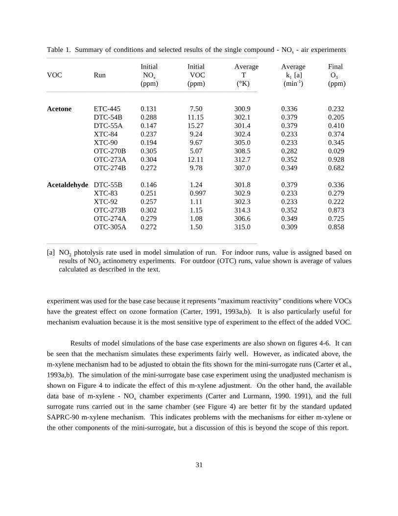
Table 1. Summary of conditions and selected results of the single compound - NOx - air experiments

Initial Initial Average Average FinalVOC Run NOx VOC T k1 [a] O3

(ppm) (ppm) (°K) (min-1) (ppm)

Acetone ETC-445 0.131 7.50 300.9 0.336 0.232DTC-54B 0.288 11.15 302.1 0.379 0.205DTC-55A 0.147 15.27 301.4 0.379 0.410XTC-84 0.237 9.24 302.4 0.233 0.374XTC-90 0.194 9.67 305.0 0.233 0.345OTC-270B 0.305 5.07 308.5 0.282 0.029OTC-273A 0.304 12.11 312.7 0.352 0.928OTC-274B 0.272 9.78 307.0 0.349 0.682

Acetaldehyde DTC-55B 0.146 1.24 301.8 0.379 0.336XTC-83 0.251 0.997 302.9 0.233 0.279XTC-92 0.257 1.11 302.3 0.233 0.222OTC-273B 0.302 1.15 314.3 0.352 0.873OTC-274A 0.279 1.08 306.6 0.349 0.725OTC-305A 0.272 1.50 315.0 0.309 0.858

[a] NO2 photolysis rate used in model simulation of run. For indoor runs, value is assigned based onresults of NO2 actinometry experiments. For outdoor (OTC) runs, value shown is average of valuescalculated as described in the text.

experiment was used for the base case because it represents "maximum reactivity" conditions where VOCs

have the greatest effect on ozone formation (Carter, 1991, 1993a,b). It is also particularly useful for

mechanism evaluation because it is the most sensitive type of experiment to the effect of the added VOC.

Results of model simulations of the base case experiments are also shown on figures 4-6. It can

be seen that the mechanism simulates these experiments fairly well. However, as indicated above, the

m-xylene mechanism had to be adjusted to obtain the fits shown for the mini-surrogate runs (Carter et al.,

1993a,b). The simulation of the mini-surrogate base case experiment using the unadjusted mechanism is

shown on Figure 4 to indicate the effect of this m-xylene adjustment. On the other hand, the available

data base of m-xylene - NOx chamber experiments (Carter and Lurmann, 1990. 1991), and the full

surrogate runs carried out in the same chamber (see Figure 4) are better fit by the standard updated

SAPRC-90 m-xylene mechanism. This indicates problems with the mechanisms for either m-xylene or

the other components of the mini-surrogate, but a discussion of this is beyond the scope of this report.

31

Table 2. Summary of conditions and results of the incremental reactivity and direct reactivity comparisonexperiments.

Initial Initial Initial Avg. Avg. Final Base [b] IRRun NOx ROGbase VOCtest T k1 [a] d(O3-NO) d(O3-NO) d(O3-NO)

(ppm) (ppmC) (ppm) (°K) (min-1) (ppm) (ppm) [c]

Mini-Surrogate - NOx with Added AcetoneETC-243 0.463 4.37 0.85 301.8 0.336 0.770 0.748 [d]ETC-245 0.504 4.65 2.19 302.3 0.336 0.886 0.757 0.059ETC-247 0.497 4.32 4.15 301.9 0.336 0.942 0.757 0.045

Mini-Surrogate - NOx with Added EthaneETC-092 0.518 3.73 17.1 301.4 0.343 0.581 0.463 0.007ETC-099 0.509 3.67 16.6 300.8 0.338 0.562 0.443 0.007ETC-235 0.494 4.56 43.7 302.0 0.336 1.006 0.754 0.006

Mini-Surrogate - NOx Base Case[e]ETC-091 0.513 3.66 - 301.3 0.344 0.433ETC-093 0.520 3.68 - 301.6 0.342 0.473ETC-098 0.517 3.58 - 301.4 0.338 0.445ETC-100 0.516 3.58 - 301.1 0.337 0.449

ETC-234 0.504 4.43 - 302.1 0.336 0.727ETC-236 0.502 4.39 - 302.0 0.336 0.705ETC-242 0.452 4.49 - 301.8 0.336 0.724ETC-244 0.484 4.31 - 302.2 0.336 0.707ETC-246 0.496 4.44 - 302.2 0.336 0.737ETC-250 0.499 4.69 - 299.9 0.336 0.746

Ethene - NOx with Added AcetoneETC-480 0.419 3.35 3.13 301.4 0.336 1.202 1.146 0.02ETC-481 0.414 3.05 5.11 301.4 0.336 1.188 1.133 0.01ETC-490 0.419 3.24 7.97 302.0 0.336 1.259 1.209 0.006

OTC-278A 0.496 1.22 2.85 311.5 0.335 1.170 0.613 0.20OTC-279B 0.526 2.00 1.27 312.6 0.345 1.317 1.271 0.04OTC-280A 0.550 2.09 1.99 310.7 0.347 1.397 1.238 0.08

Ethene - NOx with Added EthaneETC-506 0.407 3.01 50.1 300.6 0.336 1.211 1.033 0.0036

32

Table 2 (continued)

Initial Initial Initial Avg. Avg. Final Base [b] IRRun NOx ROGbase VOCtest T k1 [a] d(O3-NO) d(O3-NO) d(O3-NO)

(ppm) (ppmC) (ppm) (°K) (min-1) (ppm) (ppm) [c]

Ethene - NOx Base Case[f]ETC-479 0.409 3.36 - 301.4 0.336 1.146ETC-482 0.427 3.01 - 301.3 0.336 1.160ETC-486 0.440 3.36 - 301.4 0.336 1.082ETC-497 0.450 3.68 - 301.9 0.336 1.198ETC-505 0.401 3.15 - 301.0 0.336 1.079

OTC-278B 0.498 1.23 - 312.0 0.335 0.613OTC-279A 0.534 1.98 - 312.0 0.345 1.271OTC-280B 0.545 2.15 - 311.1 0.347 1.238

Full Surrogate - NOx with Added AcetoneDTC-28A 0.489 4.12 9.37 301.7 0.379 1.056 0.819 0.03DTC-64B 0.495 4.07 17.08 302.7 0.379 1.120 0.757 0.02

OTC-275A 0.561 4.58 10.48 317.5 0.363 1.565 1.518 0.013OTC-276B 0.571 4.46 5.81 313.7 0.355 1.498 1.405 [d]OTC-312A 0.578 4.42 2.16 315.0 0.272 1.285OTC-313B 0.494 4.14 1.86 303.4 0.247 0.900

Full Surrogate - NOx with Added EthaneOTC-312B 0.578 4.65 3.35 315.8 0.272 1.279OTC-313A 0.496 4.11 3.26 302.7 0.247 0.853

Full Surrogate - NOx Base Case[g]DTC-28B 0.492 4.14 - 301.9 0.379 0.819DTC-64A 0.494 4.25 - 302.0 0.379 0.757

OTC-275B 0.625 4.58 - 317.8 0.363 1.518OTC-276A 0.580 4.47 - 313.4 0.355 1.409OTC-314A 0.577 4.67 - 300.7 0.238 0.749OTC-314B 0.576 4.61 - 301.6 0.238 0.755

[a] NO2 photolysis rate used in model simulation of run. For indoor runs, value is assigned based onresults of NO2 actinometry experiments. For outdoor (OTC) runs, value shown is average of valuescalculated as described in the text.

[b] d(O3-NO) from base case run. For divided chamber runs with a simultaneous irradiation of a "basecase" mixture, this the d(O3-NO) from the "base case" side. For single chamber runs, this wasderived by estimating the results of a base case run for the conditions of this experiments using linearregressions derived from the results of the base case runs, as discussed by Carter et al. (1993).

33

Table 2 (concluded)

[c] Incremental reactivity in units of mol O3 per mol test VOC added[d] Effect of added VOC too small for meaningful incremental reactivity measure.[e] Representative runs carried out around the time of the added acetone or ethane experiments. For full

listing of runs used in data analysis, see Carter et al. (1993).[f] The ETC runs are representative runs carried out around the time of the added acetone experiments

in that chamber. Results of other runs were very similar. The OTC runs are the base cases for theadded acetone carried out at the same time (i.e., with the same OTC run number) but on the otherchamber side.

[g] Base cases for the added acetone carried out at the same time (i.e., with the same DTC or OTC runnumber) but on the other chamber side.

Figures 4-6 also give plots of concentration-time profiles for selected species in the added acetone

experiments, along with results of model simulations of these experiments. In addition, Figures 7 and 8

show plots, as a function of irradiation time, of the d(O3-NO) incremental reactivities which were derived

from these experiments. The error bars give the uncertainties in the measured incremental reactivities

based on estimated run to run variability and precisions of initial acetone measurements (Carter et al,

1993a). Model simulations of the incremental reactivities are also shown. It can be seen that the model

consistently and significantly overpredicts the ozone formation in the added acetone experiments, and thus

the incremental reactivity of acetone, regardless of what is being used as the base case ROG surrogate.

Acetaldehyde Experiments

As discussed above, acetaldehyde is a useful VOC for which to compare the results with

acetone because, like acetone, it is photoreactive and forms similar products in its reactions. The

conditions and selected results of the acetaldehyde - NOx and the acetaldehyde reactivity experiments are

given on Tables 1 and 2, respectively. Note that the acetaldehyde - NOx run in the DTC was carried out

at the same time as an acetone - NOx run. Much less acetaldehyde is added compared to acetone because

of its much greater reactivity.

Figure 9 shows selected results of the acetaldehyde runs carried out in the blacklight chambers.

This includes concentration-time plots for selected species in the acetaldehyde - NOx run and plots of

incremental reactivities in the acetaldehyde reactivity experiment. Results of model calculations are also

shown. It can be seen that the model gives reasonably good simulations of these data. There may be a

slight tendency for the model to overpredict acetaldehyde’s reactivity, but the discrepancy is far less than

is the case for the acetone experiments.

34

Figure 3. Experimental and calculated concentration-time profiles for selected species in the acetone- NOx runs carried out in the blacklight chambers.

35

Figure 4. Experimental and calculated concentration-time profiles for selected species in a selectedbase case run and in the added acetone reactivity experiments using the mini-surrogate inthe ETC blacklight chamber.

Ethane Experiments

Since one objective of this study is to assess the reactivities of acetone relative to those

of ethane, it is useful to also include available data for ethane. A number of incremental reactivity

experiments for ethane were carried out in the ETC using the mini-surrogate, and the results have been

presented elsewhere (Carter et al., 1993a). In addition, an ethane reactivity experiment using the ethene

surrogate has also been carried out. Table 2 gives a summary of conditions and results of the most

reliable ethane reactivity experiments carried out using the mini-surrogate and of the ethane reactivity run

using the ethene surrogate, and Figure 10 gives plots of the experimental and calculated incremental

reactivities for of these runs. (Runs carried out before the NOx injection system was modified to remove

36

Figure 5. Experimental and calculated concentration-time profiles for selected species in a selectedbase case run and in the added acetone reactivity experiments using the ethene surrogatein the ETC blacklight chamber.

nitrous acid contamination, and runs which had anomalously high reactivities which can be attributed to

an impure ethane sample, are not shown. See Carter et al., 1993.)

It can be seen that the model simulates the ethane reactivity measurements quite well. This is

expected given that ethane’s reaction mechanism is not considered uncertain, and the fact that ethane’s

major oxidation product is acetaldehyde, whose reactions the model apparently simulates quite well.

37

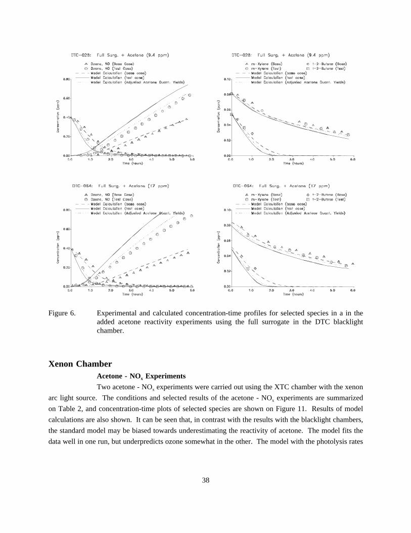
Figure 6. Experimental and calculated concentration-time profiles for selected species in a in theadded acetone reactivity experiments using the full surrogate in the DTC blacklightchamber.

Xenon ChamberAcetone - NOx Experiments

Two acetone - NOx experiments were carried out using the XTC chamber with the xenon

arc light source. The conditions and selected results of the acetone - NOx experiments are summarized

on Table 2, and concentration-time plots of selected species are shown on Figure 11. Results of model

calculations are also shown. It can be seen that, in contrast with the results with the blacklight chambers,

the standard model may be biased towards underestimating the reactivity of acetone. The model fits the

data well in one run, but underpredicts ozone somewhat in the other. The model with the photolysis rates

38

Figure 7. Experimental and calculated incremental reactivities, as a function of reaction time, in theadded acetone reactivity experiments using the mini-surrogate and the ethene surrogatein the ETC blacklight chamber.

39

Figure 8. Experimental and calculated incremental reactivities, as a function of reaction time, in theadded acetone reactivity experiments using the full surrogate in the DTC blacklightchamber.

reduced by a factor of two significantly underpredicts the ozone formation and radical levels in both these

experiments.

Acetaldehyde - NOx Experiments.

For comparison and control purposes, we also carried out acetaldehyde - NOx experiments

in this chamber. The conditions and selected results of the acetaldehyde - NOx experiments are

summarized on Table 2, and concentration-time plots of selected species are shown on Figure 12. Results

of model calculations are also shown. It can be seen that, as with the blacklight chamber runs, the model

fits the data very well.

Outdoor ChamberAcetone - NOx Experiments

A total of six acetone - NOx experiments were conducted in the outdoor chamber for this

program, of which three are used for mechanism evaluation. The conditions and selected results of these

runs are summarized on Table 2. Three of these runs were carried out on overcast days, and since our

procedures for light characterization for outdoor runs is not applicable for such conditions they were not

modeled. Concentration-time plots for selected species for the other three runs are shown on Figure 13,

where they can be compared with the model predictions. Note that run OTC-270 was carried out in

November of 1992, while the other two runs were carried out in June of 1993.

40

Figure 9. Selected experimental and calculated results for the acetaldehyde - NOx experiments andthe added acetaldehyde reactivity experiments carried out using the blacklight chambers.

41

Figure 10. Experimental and calculated incremental reactivities, as a function of reaction time, in theadded ethane reactivity experiments. All experiments were carried out in the ETCblacklight chamber.

It can be seen that the model simulation overpredicts the ozone formation and NO oxidation rates

in the winter run (OTC-270), but fits data in the summer runs reasonably well. Although the

temperatureis somewhat uncertain in run OTC-270, adjusting the temperature within its estimated

uncertainty does not significantly improve the model simulation.

Acetaldehyde - NOx Experiments.

As with the XTC, acetaldehyde - NOx experiments were carried out in the outdoor

chamber for control and comparison purposes. The conditions and selected results of the acetone - NOx

experiments are summarized on Table 2, and concentration-time plots of selected species are shown on

Figure 14. Results of model calculations are also shown. It can be seen that, as with the runs in the

42

Figure 11. Experimental and calculated concentration-time profiles for selected species in the acetone- NOx runs carried out in the xenon arc chamber.

other chamber, the model fits the data very well. This is particularly gratifying in this case, given the

greater uncertainties and difficulties in characterizing light conditions for outdoor runs. However, all the

acetaldehyde runs were carried out in the summer, and thus these data give no indication of the ability

of the model to simulate conditions in winter runs.

Acetone Reactivity Experiments

Two acetone reactivity experiments were carried out using the full surrogate and three

using the ethene surrogate. The conditions and selected results of these runs are summarized in Table 1,

concentration-time plots for selected species are given on Figure 15 for runs using the full surrogate

43

Figure 12. Experimental and calculated concentration-time profiles for selected species in theacetaldehyde - NOx runs carried out in the xenon arc chamber.

and on Figure 16 for those using the ethane surrogate. Incremental reactivity plots are given on Figure

17. Results of model simulations are also shown. Note that all of these are summer runs carried out

under clear sky conditions.

Figures 15 and 16 shows that the model consistently underpredicts the ozone formation rates in

the base case experiments. This underprediction may be due to the relatively high temperatures for these

runs, and the fact that the mechanisms for most species have not been evaluated at these higher tempera-

tures. The relatively good performance in the case of the acetaldehyde runs may be due to the fact that

the temperature dependencies for its main temperature-dependent reaction — the decomposition of PAN

— are now reasonably well characterized. One might have expected better performance in the case of

44

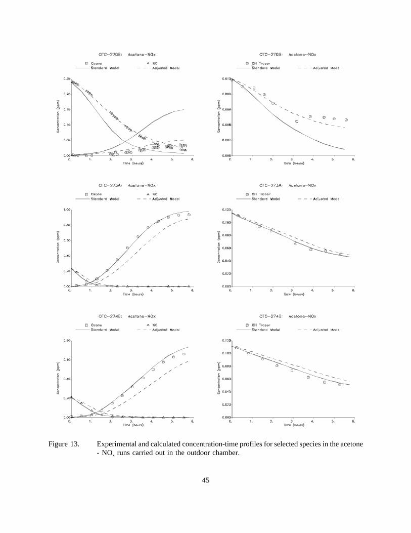
Figure 13. Experimental and calculated concentration-time profiles for selected species in the acetone- NOx runs carried out in the outdoor chamber.

45

Figure 14. Experimental and calculated concentration-time profiles for selected species in theacetaldehyde - NOx runs carried out in the outdoor chamber.

46

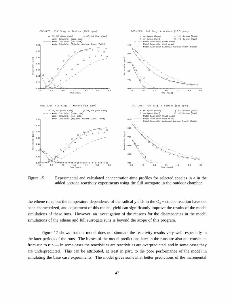
Figure 15. Experimental and calculated concentration-time profiles for selected species in a in theadded acetone reactivity experiments using the full surrogate in the outdoor chamber.

the ethene runs, but the temperature dependence of the radical yields in the O3 + ethene reaction have not

been characterized, and adjustment of this radical yield can significantly improve the results of the model

simulations of these runs. However, an investigation of the reasons for the discrepancies in the model

simulations of the ethene and full surrogate runs is beyond the scope of this program.

Figure 17 shows that the model does not simulate the reactivity results very well, especially in

the later periods of the runs. The biases of the model predictions later in the runs are also not consistent

from run to run — in some cases the reactivities are reactivities are overpredicted, and in some cases they

are underpredicted. This can be attributed, at least in part, to the poor performance of the model in

simulating the base case experiments. The model gives somewhat better predictions of the incremental

47

Figure 16. Experimental and calculated concentration-time profiles for selected species in a in theadded acetone reactivity experiments using the ethene surrogate in the outdoor chamber.

48

Figure 17. Experimental and calculated incremental reactivities, as a function of reaction time, in theadded acetone reactivity experiments carried out in the outdoor chamber.

49

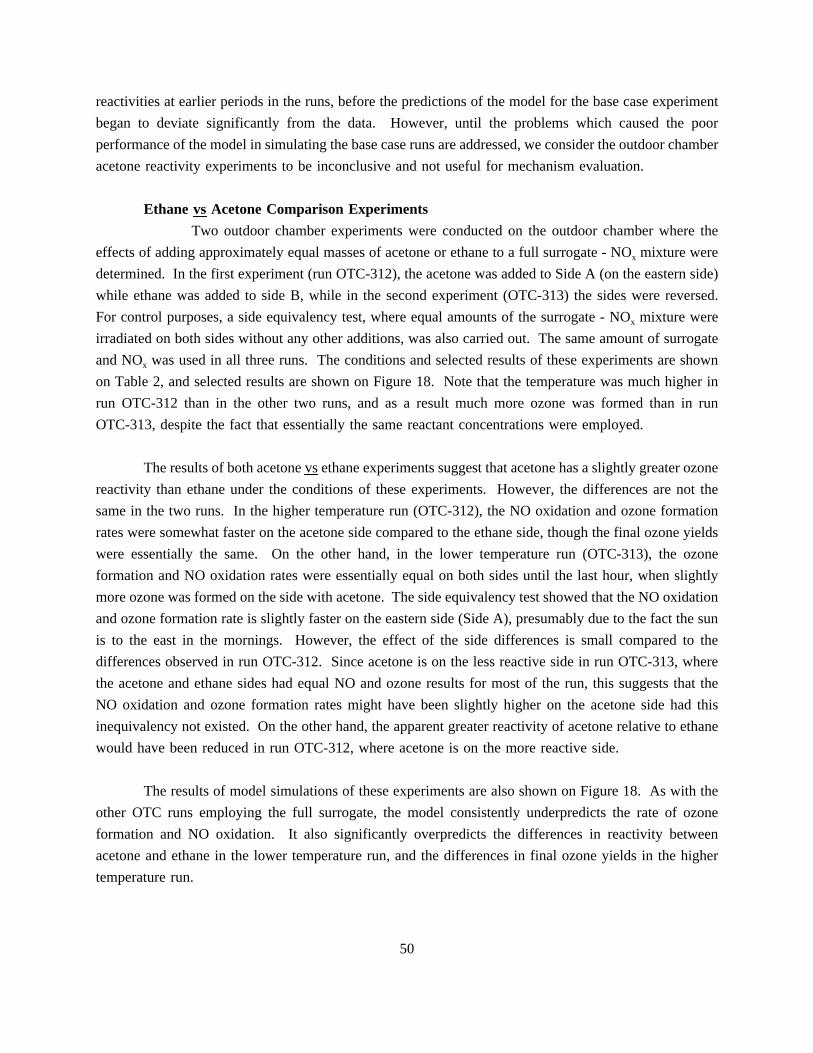
reactivities at earlier periods in the runs, before the predictions of the model for the base case experiment

began to deviate significantly from the data. However, until the problems which caused the poor

performance of the model in simulating the base case runs are addressed, we consider the outdoor chamber

acetone reactivity experiments to be inconclusive and not useful for mechanism evaluation.

Ethane vsAcetone Comparison Experiments

Two outdoor chamber experiments were conducted on the outdoor chamber where the

effects of adding approximately equal masses of acetone or ethane to a full surrogate - NOx mixture were

determined. In the first experiment (run OTC-312), the acetone was added to Side A (on the eastern side)

while ethane was added to side B, while in the second experiment (OTC-313) the sides were reversed.

For control purposes, a side equivalency test, where equal amounts of the surrogate - NOx mixture were

irradiated on both sides without any other additions, was also carried out. The same amount of surrogate

and NOx was used in all three runs. The conditions and selected results of these experiments are shown

on Table 2, and selected results are shown on Figure 18. Note that the temperature was much higher in

run OTC-312 than in the other two runs, and as a result much more ozone was formed than in run

OTC-313, despite the fact that essentially the same reactant concentrations were employed.

The results of both acetone vsethane experiments suggest that acetone has a slightly greater ozone

reactivity than ethane under the conditions of these experiments. However, the differences are not the

same in the two runs. In the higher temperature run (OTC-312), the NO oxidation and ozone formation

rates were somewhat faster on the acetone side compared to the ethane side, though the final ozone yields

were essentially the same. On the other hand, in the lower temperature run (OTC-313), the ozone

formation and NO oxidation rates were essentially equal on both sides until the last hour, when slightly

more ozone was formed on the side with acetone. The side equivalency test showed that the NO oxidation

and ozone formation rate is slightly faster on the eastern side (Side A), presumably due to the fact the sun

is to the east in the mornings. However, the effect of the side differences is small compared to the

differences observed in run OTC-312. Since acetone is on the less reactive side in run OTC-313, where

the acetone and ethane sides had equal NO and ozone results for most of the run, this suggests that the

NO oxidation and ozone formation rates might have been slightly higher on the acetone side had this

inequivalency not existed. On the other hand, the apparent greater reactivity of acetone relative to ethane

would have been reduced in run OTC-312, where acetone is on the more reactive side.

The results of model simulations of these experiments are also shown on Figure 18. As with the

other OTC runs employing the full surrogate, the model consistently underpredicts the rate of ozone

formation and NO oxidation. It also significantly overpredicts the differences in reactivity between

acetone and ethane in the lower temperature run, and the differences in final ozone yields in the higher

temperature run.

50

Figure 18. Experimental and calculated concentration-time profiles for ozone and NO, andexperimental temperature and UV light intensity data, in the acetone vsethane comparisonexperiments and the associated side equivalency test.

51

These results can be compared with the results of a very similar experiment reported by Jeffries

(1993), where equal amounts of ethane and acetone (on a per carbon basis) were added to an ROG

surrogate - NOx mix on the two sides of the University of North Carolina (UNC) outdoor chamber, and

simultaneously irriadiated. As with our OTC experiments, an equal amount of ethane was added on a per

carbon basis as the ROG surrogate, but unlike our experiments the amount of acetone added had the same

number of carbons, rather than the same mass, as the added ethane. This meant that the amount of

acetone added was 28% higher, compared to added ethane, in the UNC experiment compared to our runs.

Despite the relatively higher amount of added acetone, in the UNC experiment there was no measurable

difference in the amount of ozone formed in the added acetone side compared to the added ethane side.

Thus, either the reactivity difference was too small to be measured under the conditions of the UNC

experiment, or acetone is slightly less reactive than ethane under the conditions of that run. This is in

contrast with our results, where acetone was found to be very slightly more reactive in both experiments.

Although the runs (both ours and UNC’s) need to be reproduced before definitive conclusions can

be reached, the two OTC experiments suggest that the differences in reactivity of acetone and ethane may

be temperature dependent, with the reactivities being nearly equal at the lower temperature (which is more

representative of most ambient conditions), but with acetone becoming relatively more reactive as the

temperature increases to above 40°C (104°F). A temperature effect in the differences of reactivity might

be attributed to the relative importance of PAN formation in the photooxidation of acetone, since the

decomposition of PAN to form radicals is highly temperature dependent. However, the average

temperature in the UNC experiment was approximately 305°K, which is closer to (but slightly higher than)

the lower temperature run in this study. Thus, a temperature effect cannot be the reason for the lower

apparent reactivity of acetone relative to ethane in the UNC experiment compared to these runs. More

research concerning effects of temperature on the base case system is needed before any conclusions can

be made concerning the ability of the model to predict temperature effects on relative reactivities.

Model Simulations Using the Adjusted Acetone MechanismThe model simulations of the acetone experiments in the chambers with the blacklight and xenon

arc light sources, taken together, indicate that there is a problem with how the mechanism predicts the

acetone photolysis rate is affected by the spectrum of the light source. Although the possibility of

compensating errors can never be ruled out in model simulations of environmental chamber experiments

(Jeffries et al., 1992), the fact that the model gives reasonably good fits to the results of the acetaldehyde

experiments using the various light sources suggests that the discrepancies observed for acetone in these

chambers are not likely to be due to errors in our characterization of experimental conditions. If the

absorption cross sections are assumed to be correct (they are fairly straightforward to measure and there

is no significant inconsistency in the literature concerning them) this discrepancy can only be explained

by the model having an incorrect dependence of the quantum yields on wavelength. As discussed above,

there are inconsistencies in the literature concerning the acetone quantum yields, and the accepted values

52

are based on analyses of chemical systems which are almost as complex as these chamber experiments.

The data in the literature do not provide any guidance for reducing the discrepancy, since the

quantum yields we use in the model already are lower than any of the published values (see above). If

we had not corrected the quantum yields of Meyrahn et al. (1986), or used the higher quantum yields of

Gardner et al. (1984), the discrepancy between the model and our data from the blacklight chambers

would be even worse. Therefore, the only option we have is to make arbitrary adjustments to the quantum

yields to see if it is possible to make the model simulations more consistent with our experimental data.

We found that a factor of two downward adjustment of the photolysis rates resulted in a model

which gave excellent predictions to the experimental incremental reactivities in the blacklight chamber,

and somewhat better predictions of the results of the acetone - NOx runs using that light source. This is

shown on Figures 3-8, where the "adjusted acetone quantum yields" model uses acetone photolysis rates

which are 54% of the value used in the standard model. However, if this adjustment is made by reducing

the quantum yields by the same factor at all wavelengths, the result would be that the photolysis rate is

also reduced by a factor of ~2 in the XTC runs, which would cause a significant underprediction of ozone

formation in the acetone - NOx runs in that chamber. This is shown in Figure 11, where the dotted lines

show the model prediction where the acetone photolysis rate is reduced by approximately the same factor

that gives the best fits to the blacklight chamber runs. Since the XTC light source has a spectrum which

more closely resembles sunlight than do blacklights, this would clearly not be an acceptable adjustment

for a model to be used in ambient simulations.

To fit both the blacklight and xenon arc chamber data, it is necessary to adjust the quantum yields

such that the photolysis rates for the blacklight light source is reduced by ~2, while the rates with the

xenon arc are relatively unchanged. A possible approach for doing this is suggested by examining the

spectra of the light sources in the wavelength regions which affect acetone photolysis. Figure 1 shows

the spectra of these light sources over the full wavelength region affecting most photolysis reactions, but

shows that only a relatively narrow wavelength region, from ~290 - 320 nm, affects the photolysis of

acetone. Figure 19 shows more clearly the spectra of the light sources, and the action spectrum for

acetone, in the 300 - 320 nm wavelength region. It can be seen that the blacklights have a much lower

intensity in this wavelength region than do the xenon lights or sunlight, which means that it would have

a lower photolysis rate relative to that for NO2. This should already be taken into account in the model

simulations, since the spectra shown are used to calculate the photolysis rates. However, it also significant

to note that the ratios of intensities of the xenon light to the blacklights increase significantly with

increasing wavelength in this region. Therefore, the wavelength region affecting the acetone photolysis

rates for blacklights is higher than that affecting the photolysis rate for the xenon arc light

53

Figure 19. Top Plot shows comparison of spectra of light sources used in the environmental chamberstudies, for the wavelength range 300 - 320 nm. Bottom plot shows spectra of absorptioncross sections x quantum yields for the standard and the adjusted acetone mechanisms.

54

source. This means that decreasing the quantum yields at the higher wavelengths which are more

important in affecting the rate in the blacklight chamber while increasing them at the lower wavelengths

which are more important for the rate in the XTC might yield the desired photolysis rates under both

conditions.

An adjusted acetone action spectrum which causes the desired reduction in the acetone photolysis

rate with blacklights without significantly changing the photolysis rate in the XTC is shown on Figure 19.

This spectrum results assuming that the quantum yield is essentially constant at ~0.6 at wavelengths below

290 nm, decreases to 0.005 at 310 nm, and to essentially 0 at 320 nm, in contrast with the corrected

quantum yields of Meyrahn et al. (1986), where the quantum yields decrease more gradually with

wavelength from ~0.6 at 290 nm to 0.01 at 320 nm and 0 at 330 nm. Thus the adjusted quantum yields

are essentially the same as to those of Meyrahn et al (1986) at wavelengths≤ 280 nm, are respectively

~2 and ~1.5 times higher at 290 and 300 nm, and are significantly lower at wavelengths≥ 310 nm. (The

specific quantum yields are given with the mechanism listing in Appendix A.) The model using this set

of quantum yields is referred to as the "adjusted acetone" model. Although the set of quantum yields used

in this adjusted model is not theoretically unreasonable, we have no justification for it other than its use

results in significantly better fits to our chamber data.

The model simulations of our chamber experiments using the adjusted acetone model are shown

on Figures 3-8 for blacklight chamber runs, on Figure 11 for the XTC runs, and on Figures 13 and 15-17

for the outdoor chamber runs. As discussed above, the improvement for the blacklight chamber runs is

significant, though the adjusted model somewhat underpredicts the NO oxidation and ozone formation

rates in run ETC-445 (Figure 3). On the other hand, the adjustment does not degrade the simulation of

the acetone runs in the XTC (Figure 11); instead it slightly improves it. The adjusted model also gives

a significantly better simulation of the wintertime outdoor acetone - NOx run (OTC-270B), though the

simulation of the summertime runs (OTC-273A and OTC-274B) are not quite as good as the unadjusted

model (Figure 13). The changes in the predictions of the incremental reactivities in the outdoor runs

(Figure 17) caused by the adjustment are relatively small compared to the discrepancy between the model

calculation and the experimental data. Thus, the simulations of the outdoor runs are not sufficiently

consistent to make any conclusions concerning which mechanism performs better. However, simulations

of the better characterized indoor runs provide a much less ambiguous test of the mechanism, and the

results indicate that the adjusted model performs significantly better in simulating acetone’s reactivity and

in predicting the effects of changing the spectrum of the light source.

55

ATMOSPHERIC REACTIVITY CALCULATIONS

Since incremmental reactivities of VOCs have been shown to be highly dependent on

environmental conditions, incremental reactivities measured in environmental chamber experiments cannot

necessarily be assumed to be applicable to atmospheric conditions (Carter and Atkinson, 1989). The only

method available to obtain quantitative estimates of incremental reactivities of VOCs in ambient air

pollution episodes is to conduct airshed model simulations of the episodes. Since these simulations cannot

be any more reliable than the chemical mechanisms used, a major objective of this program was to assess

the reliability of the acetone mechanism for use in such simulations. This was discussed in the previous

sections. In this section, we discuss the results of model simulations of acetone’s incremental reactivity

in a variety of model scenarios representing ozone exceedence episodes in various areas in the United

States (Bauges, 1990), and compare the results to incremental reactivities calculated for ethane and for the

base ROG, i.e., the mixture representing total ROG emissions from all sources. Both the adjusted and the

unadjusted acetone mechanism are used.

Scenarios Used for Reactivity AssessmentThe set of airshed scenarios employed to assess acetone’s reactivity for this study is the same as

those used for calculating the MIR and other reactivity scales, as discussed previously (Carter, 1993a).

The objective is to use a set of scenarios which represents, as much as possible, a comprehensive

distribution of the environmental conditions where unacceptable levels of ozone is formed. Although a

set of scenarios has not been developed for the specific purpose of VOC reactivity assessment, the EPA

developed an extensive set of scenarios for conducting analyses of effects of ROG and NOx controls on

ozone formation using the EKMA modeling approach (Gipson et al., 1981; Gipson and Freas, 1983; EPA,

1984; Gery et al., 1987; Bauges, 1990). The EKMA approach involves use of single-cell box models to

simulate how ozone formation in one day episodes is affected by changes in ROG and NOx inputs.

Although single-cell models cannot represent realistic pollution episodes in great detail, they can represent

dynamic injection of pollutants, time-varying changes of inversion heights with entrainment of pollutants

from aloft as the inversion height increases throughout the day, and time-varying photolysis rates,

temperatures, and humidities (Gipson and Freas, 1981; EPA, 1984; Gipson, 1984; Hogo et al., 1988).

Thus, they can be used to simulate a wide range of the chemical conditions which affect ozone formation

from ROG and NOx. These are the same as those affecting VOC reactivity. Therefore, at least to the

extent they are suitable for their intended purpose, an appropriate set of EKMA scenarios should also be

suitable for assessing methods to develop reactivity scales encompassing a wide range of conditions.

56

Base Case Scenarios

The set of EKMA scenarios used in this study were developed by the United States EPA

for assessing how various ROG and NOx control strategies would affect ozone nonattainment in various

areas of the country (Bauges, 1990). The characteristics of these scenarios and the methods used to derive

their input data are described in more detail elsewhere (Bauges, 1990; Carter, 1993a). Briefly, 39 urban

areas in the United States were selected based on geographical representativeness of ozone nonattainment

areas and data availability, and a representative high ozone episode was selected for each. The initial

NMOC and NOx concentrations, the aloft O3 concentrations, and the mixing height inputs were based on

measurement data for the various areas, the hourly emissions in the scenarios were obtained from the

National Acid Precipitation Assessment Program emissions inventory (Bauges, 1990), and biogenic

emissions were also included. Table 3 gives a summary of the urban areas represented and other selected

characteristics of the scenarios.

Several changes to the scenario inputs were made based on discussions with the California ARB

staff and others (Carter, 1993a). Two percent of the initial NOx and 0.1% of the emitted NOx in all the

scenarios was assumed to be in the form of HONO. The photolysis rates were calculated using solar light

intensities and spectra calculated by Jeffries (1991b) for 640 meters, the approximate mid-point of the

mixed layer during daylight hours. The composition of the NMOCs entrained from aloft was based on

the analysis of Jeffries et al (1989a). The composition of the initial and emitted reactive organics was

derived as discussed below. Complete listings of the input data for the scenarios are given elsewhere

(Carter, 1993a).

This set of 39 EKMA scenarios are referred to as "base case" to distinguish them from the

scenarios derived from them by adjusting NOx inputs to yield standard conditions of NOx availability as

discussed below. No claim is made as to the accuracy of these scenarios in representing any real episode,

but they are a result of an effort to represent, as accurately as possible given the available data and the

limitations of the formulation of the EKMA model, the range of conditions occurring in urban areas

throughout the United States. When developing general reactivity scales it is more important that the

scenarios employed represent a realistic distribution of chemical conditions than any accurately represent-

ing the details of any one particular episode.

The Base ROG mixture is the mixture of reactive organic gases used to represent the chemical

composition of the initial and emitted anthropogenic reactive organic gases from all sources in the

scenarios. Consistent with the approach used in the original EPA scenarios, the same mixture was used

for all scenarios. The speciation for this mixture was derived by Croes (1991) based on an analysis of

the EPA database (Jeffries et al. 1989a) for the hydrocarbons and the 1987 Southern California Air Quality

Study (SCAQS) database for the oxygenates (Croes et al., 1993; Lurmann et al., 1992). This mixture

consists of 52% (by carbon) alkanes, 15% alkenes, 27% aromatics, 1% formaldehyde, 2% higher

57

Table 3. Summary of conditions of base case scenarios used for atmospheric reactivity assessment.

Calc. ROG NOx Final Init.+Emit AloftCity, State Max O3 /NOx /NOx

MOR Height Base ROG O3(ppb) (km) (mmol m-2) (ppb)

Atlanta, GA 174 7.3 0.7 2.1 12 63Austin, TX 171 9.3 0.5 2.1 11 85Baltimore, MD 304 5.2 1.1 1.2 17 84Baton Rouge, LA 235 6.8 1.0 1.0 11 62Birmingham, AL 233 6.9 0.6 1.8 13 81Boston, MA 191 6.5 0.6 2.6 14 105Charlotte, NC 142 7.8 0.3 3.0 7 92Chicago, IL 273 11.6 0.5 1.4 25 40Cincinnati, OH 192 6.4 0.8 2.8 17 70Cleveland, OH 239 6.6 1.0 1.7 16 89Dallas, TX 192 4.7 1.3 2.3 18 75Denver, CO 195 6.3 1.2 3.4 29 57Detroit, MI 229 6.8 0.8 1.8 17 68El Paso, TX 177 6.6 1.1 2.0 12 65Hartford, CT 166 8.4 0.5 2.3 11 78Houston, TX 291 6.1 1.0 1.7 25 65Indianapolis, IN 201 6.6 0.9 1.7 12 52Jacksonville, FL 152 7.6 0.7 1.5 8 40Kansas City, MO 151 7.1 0.6 2.2 9 65Lake Charles, LA 282 7.4 0.7 0.5 7 40Los Angeles, CA 546 7.6 1.0 0.5 23 100Louisville, KY 203 5.5 0.9 2.5 14 75Memphis, TN 218 6.8 0.7 1.8 15 58Miami, FL 131 9.6 0.4 2.7 9 57Nashville, TN 163 8.1 0.5 1.6 7 50New York, NY 350 8.1 0.8 1.5 39 103Philadelphia, PA 230 6.2 1.0 1.8 19 53Phoenix, AZ 258 7.6 1.0 3.3 40 60Portland, OR 161 6.5 0.7 1.6 6 66Richmond, VA 225 6.2 0.8 1.9 16 64Sacramento, CA 194 6.6 0.9 1.1 7 60St Louis, MO 301 6.1 1.1 1.6 26 82Salt Lake City, UT 179 8.5 0.6 2.2 11 85San Antonio, TX 126 3.9 1.1 2.3 6 60San Diego, CA 186 7.1 1.0 0.9 8 90San Francisco, CA 222 4.8 1.8 0.7 25 70Tampa, FL 217 4.4 1.1 1.0 8 68Tulsa, OK 216 5.3 0.9 1.8 15 70Washington, DC 268 5.3 0.9 1.4 13 99

58

aldehydes, 1% ketones, and 2% acetylene. The detailed composition of this mixture is given elsewhere

(Carter, 1993a).

Maximum Incremental Reactivity (MIR) and Maximum Ozone Reactivity (MOR) Scenarios

Incremental reactivities in the base case scenarios would be expected to vary widely, since

incremental reactivities depend on the ROG/NOx ratio, and that ratio varies widely among the base case

scenarios. To obtain reactivity scales for specified NOx conditions, a separate set of scenarios, designated

MIR (for maximum incremental reactivity) and MOR (for maximum ozone reactivity) were developed

(Carter, 1991, 1993a,b). In the MIR scenarios, the NOx inputs were adjusted so the base ROG mixture

(and most other VOCs) have their highest incremental reactivity. In the MOR scenarios, the NOx inputs

were adjusted to yield the highest ozone concentration. The changes in the base case ROG/NOx ratios

which yielded the MOR scenarios are given in Table 3. As discussed by Carter (1993a,b) the MIR

ROG/NOx ratios are ~1.4 times higher than MOR ratios in all cases.

NOx Conditions in the Base Case Scenarios

As indicated above, the variability of ROG/NOx ratios in the base case scenarios suggest

a variability of reactivity characteristics in the base case scenarios. However, as discussed previously

(Carter, 1993a,b), the ROG/NOx ratio is also variable in the MIR or MOR scenarios, despite the fact that

the NOx inputs in these scenarios are adjusted to yield a specified reactivity characteristic. Thus, the

ROG/NOx ratio, by itself, is not necessarily a good predictor of reactivity characteristics of a particular

scenario. The NOx/NOxMOR ratio is a much better predictor of this, with values greater than 1 indicating

relatively high NOx conditions where ozone formation is more sensitive to VOCs, and values less than 1

indicating NOx-limited conditions. NOx/NOxMOR ratios less than 0.7 represent conditions where NOx

control is a more effective ozone control strategy than ROG control (Carter, 1993a,b). Note that more

than half of the base case scenarios represent NOx-limited conditions, and ~25% of them represent

conditions where NOx control is more beneficial than VOC control. A relatively small number of

scenarios represent MIR or near MIR conditions. However, as discussed elsewhere (Carter, 1993a,b), this

set of scenarios is based on near-worst-case conditions for ozone formation in each of the airsheds. Had

scenarios representing less-than-worst-case conditions been included, one might expect a larger number

of MIR or near MIR scenarios. This is because NOx is consumed more slowly on days with lower light

intensity or temperature, and thus the scenario is less likely to become NOx-limited.

Incremental and Relative ReactivitiesThe incremental reactivity of a VOC in an airshed scenario is the change in ozone caused by

adding the VOC to the emissions, divided by the amount of VOC added, calculated for sufficiently small

amounts of added VOC that the incremental reactivity is independent of the amount added. The procedure

used to calculate incremental reactivities in a scenario was as discussed in detail elsewhere (Carter, 1993a).

The incremental reactivities depend on how the amount of VOC added are quantified. In this work, the

59

added VOC was quantified on a mass basis, since this is how VOCs are regulated. In addition, the

incremental reactivities also depend on how ozone impacts are quantified (Carter, 1993a,b). In this work,

two different ozone quantifications were used, resulting in two different incremental reactivities being

calculated for a VOC in a scenario. These are discussed below.

The "Ozone Yield" incremental reactivitiesmeasure the effect of the VOC on the total amount

of ozone formed in the scenario at the time of its maximum concentration. In this work, this is quantified

as grams O3 formed per gram VOC added. This gives the same ratios of incremental reactivities as

reactivities calculated from peak ozone concentrations, but is preferred because it permits magnitudes of

reactivities in scenarios with differing dilutions to be compared on the same basis. Most previous recent

studies of incremental reactivity (Dodge, 1984; Carter and Atkinson, 1987, 1989, Chang and Rudy, 1990;

Jeffries and Crouse, 1991) have all been based on ozone yield or peak ozone concentration reactivities.

The ozone yield incremental reactivities do not necessarily measure the effect of the VOC on

exposure of unacceptable levels of ozone because it does not measure how long high levels of ozone is

present. A quantification which reflects this is integrated ozone over the standard, which is defined as the

sum of the hourly ozone concentrations for the hours when ozone exceeds the standard in the base case

scenarios (Carter 1993a,b). In the previous work (Carter, 1993a,b), we used the California ozone standard

of 90 ppb, but in this work we will use the national standard of 0.12 ppm. Reactivities relative to this

quantification of ozone are referred to by the abbreviation "IntO3>0.12" reactivities.

Relative reactivitiesare ratios of incremental reactivities to incremental reactivities of some

standard VOC or mixture. Since these are the quantities which usually are the most relevant to control

strategy applications, the results in this work will be given in terms of relative reactivities. In our previous

work (Carter 1991, 1993a,b), we used the incremental reactivity of the base ROG mixture, i.e., the mixture

representing ROG pollutants from all sources, as the standard to define relative reactivities. To be

consistent with the terminology in the previous work, if the term "relative reactivity" is used without

qualifier it refers to incremental reactivities relative to the base ROG mixture. However, because of the

tendency within the EPA to consider ethane as the standard to define exempt vscontrolled VOCs, we will

also give reactivity ratios where ethane is used as the standard.

Reactivity ScalesA reactivity scale is a set of incremental or relative reactivities for a particular scenario or group

of scenarios. Two types of reactivity scales will be discussed here, "base case" scales and adjusted NOx

scales. Base case scales are simply the set of incremental or relative reactivities in the 39 base case

scenarios. Two sets of base case scales are derived — those based ozone yield reactivities and those based

on IntO3>0.12 reactivities. In the previous work (Carter, 1991, 1993a,b) we derived various multi-scenario

scales from the individual base case scales by averaging or other procedures, to evaluate alternative

60

approaches for developing single reactivity scales for applications requiring single scales. However, the

decision of whether to exempt a VOC should not be made based on relative reactivities of a single scale,

but on a knowledge of the range of relative reactivities for a variety of conditions. Thus in this work we

present the distribution of base case relative reactivities for the 39 individual scenarios rather than

developing aggregated or optimum scales which represent the distribution by single numbers.

The adjusted NOx incremental reactivity scales refer to the MIR (maximum incremental reactivity)

or the MOIR (maximum ozone incremental reactivity) scales. These consist of averages of incremental

reactivities MIR or MOIR scenarios, respectively. Relative reactivities in these scales are ratios of

incremental reactivities in these scales. Reactivities in the MIR scale are of interest because the California

Air Resources Board utilized an MIR scale to calculate reactivity adjustment factors in its clean fuels/low

emissions vehicle regulations (CARB, 1991). The justification for using this scale in applications

requiring a single scale (such as the CARB vehicle regulations) is that it reflects conditions where ozone

is most sensitive to changes in VOC emissions, and complements NOx control, which is most effective

for reducing ozone under conditions where the MIR scale is least applicable (Carter, 1993a,b). The MOIR

scale is preferred by many as an alternative for such applications because it reflects conditions which are

most favorable for ozone, and is more representative of the distribution of conditions in the base case

scenarios (Carter 1993a,b). Most other alternative reactivity scales which might be appropriate for

assessing VOC control strategies (i.e., excluding scales representing highly NOx-limited conditions where

ozone is more sensitive to NOx than VOCs) tend to fall in the range defined by the MIR and MOIR scales.

Note that the MIR, MOIR and base case scales derived in this work are somewhat different from

those calculated previously (Carter, 1993a,b) because an updated chemical mechanism was used. Table

4 gives the MIR and MOIR incremental reactivities using the mechanism employed in this work and

compares them with those calculated previously (Carter, 1993a,b), which were derived using the

SAPRC-90 mechanism. The updates to the mechanism result in higher incremental reactivities for all

species except for formaldehyde, acetone, and benzaldehyde, higher relative reactivities for internal

alkenes, alkanes other than methane and benzene, lower relative reactivities for formaldehyde, acetone,

and benzaldehyde, and slightly lower relative reactivities for most other species. The decrease in relative

reactivity for formaldehyde and acetone, and increase for internal alkenes, are directly attributable to

changes in their mechanisms as discussed above.

Calculated Relative Reactivities of Acetone and EthaneTable 5 gives a tabulation of the relative reactivities of acetone and ethane in the various base case

and MIR and MOIR reactivity scales calculated using the updated mechanism. Distribution plots of the

relative reactivities of acetone and ethane in the base case scenarios are shown on Figure 20, Figures 21

gives distribution plots of the acetone/ethane incremental reactivity ratio for the base case scenarios, and

61

Table 4. Comparison of incremental and relative reactivities in the MIR and MOIR scales calculatedusing the updated and the SAPRC-90 mechanisms.

Compound MIR Scale [a] MOIR Scale [a]SAPRC-90 Updated Change (%) SAPRC-90 Updated Change (%)

IR IR IR RR IR IR IR RR

CO 0.054 0.061 13% -3% 0.038 0.040 4% -10%

Methane 0.0150 0.016 10% -6% 0.0093 0.0099 6% -8%Ethane 0.25 0.30 21% 4% 0.17 0.20 24% 6%n-Butane 1.02 1.26 23% 5% 0.66 0.83 26% 9%n-Octane 0.60 0.83 37% 17% 0.41 0.57 38% 19%iso-Octane 0.93 1.16 25% 7% 0.54 0.72 33% 15%n-Decane 0.46 0.68 46% 25% 0.31 0.47 51% 30%

Ethene 7.4 8.3 12% -4% 3.2 3.4 6% -9%Propene 9.4 11.2 18% 1% 3.8 4.3 13% -3%trans-2-Butene 10.0 13.5 35% 16% 3.8 4.7 25% 7%Isobutene 5.3 6.0 13% -3% 1.9 2.0 4% -10%1-Hexene 4.4 5.7 30% 11% 1.7 2.3 31% 13%

Benzene 0.42 0.60 42% 22% 0.138 0.20 48% 27%Toluene 2.7 3.2 16% -1% 0.63 0.69 10% -5%m-Xylene 8.2 8.8 8% -8% 2.5 2.5 2% -12%135-TM-Benzene 10.1 11.3 11% -5% 3.1 3.2 4% -11%

Methanol 0.56 0.63 11% -5% 0.28 0.29 4% -11%Ethanol 1.34 1.6 21% 4% 0.72 0.90 24% 7%

Formaldehyde 7.2 7.0 -2% -16% 2.1 1.9 -11% -23%Acetaldehyde 5.5 6.3 15% -2% 2.2 2.4 12% -3%

Acetone [b] 0.56 0.49 -13% -25% 0.20 0.19 -7% -20%

Benzaldehyde -0.57 -0.24 58% 64% -1.24 -1.41 -14% 2%Cresols 2.3 2.6 13% -3% -0.58 -0.59 3% -12%

Base ROG Mix 3.1 3.7 17% 0% 1.17 1.36 16% 0%

[a] IR = incremental reactivities in units of grams O 3 per gram VOC; RR = reactivityrelative to base ROG mixture.

[b] Standard acetone mechanism.

62

Table 5. Relative ozone yield and IntO3>0.12 reactivities and reactivity ratios for acetone and ethane inthe base case scenarios and the MIR and MOIR scales.

Reactivities Relative to Base ROGScenario Base ROG Ozone Yield Reactivities IntO3 > 0.12 Reactivitiesor Scale IR [a] Ethane Acetone Acetone Ethane Acetone Acetone

(Standard) (Adjusted) (Standard) (Adjusted)

Base Case Scenarios

ATL GA 0.93 0.17 0.144 0.128 0.130 0.123 0.107AUS TX 0.74 0.20 0.147 0.133 0.149 0.117 0.103BAL MD 1.7 0.132 0.142 0.123 0.086 0.126 0.104BAT LA 1.00 0.142 0.136 0.117 0.103 0.117 0.098BIR AL 0.80 0.24 0.17 0.16 0.129 0.120 0.103BOS MA 0.79 0.21 0.147 0.136 0.143 0.120 0.106CHA NC 0.60 0.22 0.16 0.145 0.18 0.138 0.125CHI IL 0.38 0.24 0.18 0.16 0.135 0.115 0.096CIN OH 1.14 0.19 0.141 0.129 0.120 0.112 0.096CLE OH 1.25 0.139 0.135 0.118 0.092 0.115 0.096DAL TX 2.5 0.103 0.125 0.104 0.085 0.114 0.094DEN CO 1.7 0.097 0.132 0.111 0.074 0.122 0.100DET MI 1.02 0.20 0.144 0.130 0.121 0.114 0.098ELP TX 1.5 0.104 0.130 0.107 0.081 0.118 0.095HAR CT 0.86 0.21 0.15 0.140 0.16 0.130 0.116HOU TX 1.21 0.17 0.140 0.125 0.104 0.111 0.094IND IN 1.37 0.15 0.131 0.115 0.110 0.116 0.098JAC FL 0.82 0.16 0.137 0.120 0.143 0.126 0.109KAN MO 1.10 0.20 0.143 0.131 0.16 0.124 0.111LAK LA 0.60 0.21 0.15 0.138 0.135 0.118 0.099LOS CA 0.77 0.121 0.128 0.110 0.075 0.106 0.084LOU KY 1.36 0.18 0.144 0.129 0.128 0.119 0.103MEM TN 0.89 0.20 0.15 0.138 0.126 0.119 0.102MIA FL 0.61 0.19 0.148 0.133 0.18 0.141 0.127NAS TN 0.81 0.24 0.17 0.16 0.19 0.149 0.135NEW NY 0.45 0.16 0.130 0.114 0.084 0.100 0.080PHI PA 1.20 0.16 0.135 0.121 0.105 0.116 0.099PHO AZ 1.41 0.144 0.139 0.121 0.093 0.115 0.095POR OR 1.08 0.18 0.139 0.125 0.142 0.124 0.108RIC VA 1.11 0.18 0.144 0.132 0.110 0.120 0.103SAC CA 1.29 0.16 0.15 0.132 0.125 0.133 0.115SAI MO 1.42 0.124 0.137 0.119 0.081 0.120 0.101SAL UT 0.94 0.19 0.16 0.140 0.128 0.125 0.108SAN TX 1.8 0.124 0.126 0.107 0.120 0.124 0.105SDO CA 0.98 0.110 0.109 0.090 0.085 0.099 0.078SFO CA 1.9 0.053 0.146 0.116 0.050 0.142 0.114TAM FL 1.8 0.123 0.132 0.113 0.094 0.119 0.099TUL OK 1.27 0.17 0.137 0.124 0.120 0.118 0.103WAS DC 1.07 0.19 0.146 0.132 0.110 0.112 0.096

Average 1.13 0.166 0.142 0.126 0.118 0.120 0.103

Adjusted NO x Scales

MIR Scale 3.7 0.082 0.133 0.110MOIR Scale 1.36 0.150 0.139 0.121

[a] Incremental reactivity in units of gm O3/gm VOC.

63

Figure 20. Distribution plots of ozone yield and IntO3>0.12 reactivities, relative to the base ROGmixture, for acetone and ethane in the base case scenarios.

64

Figure 21. Distribution plots of ratios of ozone yield and IntO3>0.12 reactivities ofacetone relative to ethane for the base case scenarios.

Figure 22. Plots of ratios of ozone yield reactivities of acetone relative to ethane against theincremental reactivity of the base ROG for the base case scenarios. Reactivity ratios andranges of base ROG reactivities for the MIR and MOIR scales are also shown.

65

figure 22 plots the acetone/ethane reactivity ratios against the incremental reactivity of the base ROG.

Reactivities of acetone were calculated both using the standard updated mechanism and using the

mechanism with the acetone quantum yields adjusted to fit the blacklight and xenon arc chamber data as

discussed above.

It can be seen that the adjustment to the acetone mechanism to fit the chamber data causes a slight

(~13%) reduction in the incremental and relative reactivity of acetone. This is a fairly small difference

compared to the variability of its relative reactivity or reactivity relative to ethane. The differences

between these two calculations can be thought of as an indication of the lower limit to the chemical

uncertainty in calculations of acetone’s reactivity.

Figures 21 and 22 show that acetone is less reactive than ethane in a majority of the base case

scenarios, though there are a few scenarios where acetone is slightly more reactive, and one where the

unusually low relative reactivity of ethane results in an unusually high acetone/ethane reactivity ratio. The

reactivity ratio in this case does not appear to be significantly affected by how O3 is quantified — though

it should be noted that this is not the case for all VOCs (Carter 1993a,b). Figure 22 shows that the

reactivity ratio tends to increase as the reactivity ratio increases above the range which is characteristic

of maximum ozone conditions. Thus, although acetone is of equal or lesser reactivity to ethane in most

scenarios, its reactivity relative to ethane tends to increase as the scenario becomes more sensitive to VOC

emissions. Because of this, incremental reactivity of acetone in the MIR scale is calculated to be 1.3 or

1.6 times higher than that of ethane, depending on whether the quantum yields are adjusted to fit the

chamber data. However, all but one of the base case scenarios have lower reactivity ratios than in the

MIR scale. The distribution of reactivity ratios in the base case scenarios is better represented by the

reactivity ratio in the MOIR scale, where acetone is calculated to be slightly less reactive than ethane.

An alternative — and we believe more relevant — standard for assessing whether to regulate

emissions of a compound is its reactivity relative to the mix of all other emitted VOCs, or the base ROG

mixture. Figure 20 shows that the relative reactivities of acetone varies over a much narrower range than

those for ethane, though the variation is somewhat less when ozone is quantified by integrated O3 over

the standard. The range of ozone yield relative reactivities are 0.05 - 0.24 for ethane and 0.11 - 0.18 for

acetone with the more reactive standard mechanism. Thus acetone with the standard mechanism is

between 5.6 - 9 times less reactive in terms of ozone yields than the base ROG, while ethane is between

4 - 20 times less reactive. For ozone yield reactivities, the ranges of relative reactivities are 0.074 - 0.19

for ethane and 0.10 - 0.15 for the standard acetone mechanism. Thus acetone with the standard

mechanism is between 7 - 10 times less reactive in terms of integrated ozone over the standard than the

base ROG, while ethane is 5 - 13 times less reactive. The MIR and MOIR relative reactivities are within

these ranges.

66

It is interesting to note that the scenarios where acetone looks the most reactive compared to

ethane are not necessarily the same as those where acetone has the highest reactivity relative to the base

ROG mixture. From Figure 21 it can be seen that there is one scenario where the acetone/ethane

reactivity ratio is unusually high, being 3 for the unadjusted mechanism. However, Table 5 shows that

the corresponding ozone yield relative reactivity for the unadjusted acetone mechanism in that scenario

is only 0.146, which is very close to the average for all scenarios. Thus the high acetone/ethane reactivity

ratio in that case is due entirely to an unusually low relative reactivity for ethane. Furthermore, the

scenario with the highest relative reactivity for acetone has an acetone/ethane reactivity ratio of ~0.75 for

the standard mechanism, which is lower than average. In general, because the relative reactivity of ethane

is so much more variable than that of acetone (as shown on Figure 20), it is the reactivity of ethane which

is the primary factor which determines the reactivity of acetone relative to ethane.

67

CONCLUSIONS

The decision whether it is appropriate to regulate a compound as an ozone precursor requires a

qualitative assessment of its reactivity relative to ozone formation under a variety of environmental

conditions. This requires developing and experimentally validating a chemical mechanism for the

compounds relevant atmospheric reactions, which can then be used in airshed models to predict its

atmospheric reactivity. Although mechanisms for the atmospheric reactions of acetone have been available

for some time, until this study there have been no reliable data available to evaluate their accuracy when

used in such models. The major objective of this study was to provide the data needed for this purpose.

The data base which was developed to evaluate the mechanism of acetone is now more extensive

than that for a vast majority of the other VOCs emitted into the atmosphere, including many which are

far more important in contributing to the ozone problem. Acetone has been studied in NOx-air

environmental chamber irradiations by itself and in the presence of other reactive VOCs, and experiments

utilizing a variety of light sources, including natural sunlight and artificial lights closely resembling natural

sunlight. Although the incremental reactivity experiments in the outdoor chamber are inconclusive because

of the inability of the model to simulate the base case conditions, the outdoor chamber experiments with

acetone in the absence of other added VOCs, and the wide variety of indoor chamber experiments, provide

a useful data base for evaluating acetone’s mechanism. The indoor runs using the blacklights provide

information concerning the effects of acetone on ozone formation under a wide variety of conditions, and

the runs using the xenon arc light source provide information concerning acetone which more closely

resembles sunlight. The difference in spectral distribution of the blacklight and xenon arc light sources

provide a valuable means to test the model for how the photolysis of acetone depends on light spectrum.

This is important because the spectrum of ambient sunlight is not constant, it varies significantly

depending on the time of day, day of year, and the extent of atmospheric haze and the tropospheric ozone

column.

An examination of the recent literature and reviews concerning the atmospheric reactions of

acetone indicate that the mechanism we have previously used for acetone (Carter, 1990) needed to be

updated in some respects. The greatest uncertainty in the acetone photooxidation mechanism is the

quantum yields for its photolysis, concerning which the data in the literature are not in agreement. The

evaluations (e.g., Atkinson et al., 1992) recommend the models use the data of Meyrahn et al. (1986), but

our model simulations of their experiments indicate that the quantum yields in longest wavelengths (where

sunlight and blacklights are more intense) are unreliable and need correction. The acetone mechanism

used in our model was updated to be consistent with the latest evaluations in the literature, and to

incorporate the estimated correction to the quantum yield data of Meyrahn et al (1986). These corrections

68

had a tendency to make acetone somewhat less reactive than was previously predicted, but still of

comparable reactivity to ethane.

The updated mechanism was found to simulate reasonably well the results of the experiments

using the indoor chamber light source most closely resembling sunlight and the outdoor chamber runs

which were conducted during the summer. However, this mechanism consistently overpredicted the rate

of ozone formation in the blacklight chamber experiments and also overpredicted the ozone formation in

the wintertime acetone - NOx run in the outdoor chamber. It is considered unlikely that this is due to

incorrect characterization of the blacklight intensity or spectra, because the model could give good

simulations of the photochemical reactivity of acetaldehyde, a VOC which photolyzes in a similar

wavelength region as acetone. Thus it appears likely that the problem is that the model incorrectly

represents how the acetone photolysis quantum yields depend on wavelength.

An adjusted version of the updated acetone mechanism was developed which was considerably

more successful in simulating the data base developed in this study. The adjustment involves assuming

that the quantum yields fall off with increasing wavelength much more rapidly than indicated by the data

of Meyrahn et al. (1986), but that the fall off begins at a slightly longer wavelength. Although this

adjustment is not theoretically unreasonable, there is no basis for it other than fitting these environmental

chamber data, which are highly complex chemical systems with a number of other potential sources of

error. The possibility that the problem may be due to an incorrect characterization of the effect of the

mercury lines in the blacklight light source cannot be entirely ruled out. Therefore, in the assessment of

the reactivities of acetone in the atmosphere, both the unadjusted (or standard) mechanism and the adjusted

acetone mechanism were used in the model calculations. A comparison of the predictions of the two

mechanisms give an indication of the approximate minimum magnitude of the effects of chemical

mechanistic uncertainties associated with calculations of acetone’s atmospheric reactivity.

It was found that the adjustment to the acetone quantum yields to fit our chamber data caused an

approximately 13% reduction in the calculated incremental reactivity of acetone under atmospheric

conditions. This is a relatively small effect compared to the extent to which the relative reactivity of

acetone varied with atmospheric conditions. Thus it is concluded that although there are uncertainties in

acetone’s quantum yields, the effect of this uncertainty is not large enough to substantively affect

conclusions concerning the range of acetone’s effect on ozone production under conditions represented

by the model scenarios we employed. However, the effect may be larger in model simulations of

wintertime conditions, since the adjustment has the greatest effect under lighting conditions which have

relatively low intensity in the UV. Since all the scenarios used in this study were based on worst case

or near-worst case conditions, conditions of low UV intensity are not well represented.

69

The model simulations indicate that acetone is slightly less reactive than ethane in a majority of

the scenarios representing worst-case or near-worst-case conditions. However, there was one scenario

where the ethane was calculated to have an unusually low relative reactivity, resulting in acetone being

calculated to be more reactive than ethane by factors of 2-3, depending on whether or not the adjusted

quantum yields are used. In general, acetone becomes increasingly more reactive relative to ethane as NOx

conditions approach those yielding the highest incremental reactivities, with the result being that acetone

has a slightly higher (by a factor of 1.3 to 1.6, depending on the quantum yields) MIR incremental

reactivity than ethane. On the other hand, in the MOIR scale, which represents NOx conditions most

favorable for ozone formation, acetone is calculated to be slightly less reactive than ethane, regardless of

which set of quantum yields are used. In general, the MIR and MOIR scales represent the range of

conditions which are appropriate to consider when evaluating relative reactivities of VOC for control

strategy purposes (Carter, 1991; 1993a,b).

However, other than considerations of precedence, the reactivity of acetone relative to ethane is

of essentially no practical relevance. The two chemicals have vastly different physical properties and

come from quite different types of sources, and to our knowledge no substitutions of acetone for ethane

(or vise-versa) are being contemplated. If a reactive VOC is exempted, and if it is not used primarily as

a substitute for more reactive VOCs, the net effect would be that there would have to be a slightly greater

controls on all other (non-exempt) VOCs to achieve the same air quality gains. Thus, in effect, the

proposal to exempt a VOC is equivalent to proposing to substitute it for the base ROG mixture.

Therefore, the more relevant consideration when considering whether to exempt acetone is its reactivity

compared to the base ROG mixture.

When compared on the basis of reactivities relative to the base ROG mixture, a somewhat

different picture is obtained concerning the relative impacts of acetone and ethane on ozone formation.

In particular, the relative reactivity (i.e., incremental reactivity relative to the base ROG) of acetone is

found to vary over a considerably narrower range than is the case for ethane. Indeed, it is the variability

of the relative reactivity of ethane, not acetone, which causes the variability of the acetone/ethane

reactivity ratios among the scenarios. For example, the scenario with the most extreme acetone/ethane

reactivity ratios (of 2-3) had relative reactivities for acetone very close to the average. The minimum,

maximum, and average relative reactivities we obtained are summarized on Table 6, where they are

compared with relative reactivities in the MIR and MOIR scales. It should be noted that the base case

scenarios were designed to represent near-worst-case conditions only, and the results may be more variable

if a greater variety of scenarios were included. However, these scenarios are representative of a wide

variety of conditions which need to be considered when assessing effects of VOC controls.

70

Table 6. Summary of reactivities of acetone and ethane relative to the base ROG mixture.

Based on effect on O3 Yield Based on Integrated O3 > 0.12 ppmAcetone Acetone Ethane Acetone Acetone Ethane

(standard) (adjusted) (standard) (adjusted)

Base caseMinimum 0.11 0.09 0.05 0.10 0.07 0.05Maximum 0.18 0.16 0.24 0.15 0.14 0.19Average Base 0.14±0.01 0.13±0.02 0.17±0.04 0.12±0.01 0.10±0.010.12±0.03

MIR Scale 0.13 0.11 0.08MOIR Scale 0.14 0.12 0.15

We believe the type of data on Table 6 provides a more appropriate basis for deciding whether

it is appropriate to exempt acetone or ethane. Note that when the EPA decided to exempt ethane, in effect

it decided it was not necessary to regulate emissions of a VOC which could be almost 25% asreactive as

the average of all emissions in terms of peak ozone concentrations, and almost 20% as reactive in terms

of effect on integrated ozone over the standard. When looked at this way, exempting a compound which

is calculated to be no more than 20% as reactive in terms of peak ozone, or 15% as reactive in terms of

integrated ozone over the standard, does not appear to be an inconsistent policy.

To conclude, when considering whether a VOC should be exempted from regulation as an ozone

precursor, the most appropriate factor to consider is its relative reactivity, i.e., its reactivity relative to the

mixture of all other VOC emissions. The results of this study indicate that the difference in relative

reactivities between ethane and acetone is less than the variability of their relative reactivities from

scenario to scenario. On this basis, it can be concluded the acetone and ethane can be considered to have

essentially the same reactivity to within their variability with environmental conditions. However, it

should be emphasized that the scenarios we employed were designed to represent near-worst-case

conditions only, and the variability may be greater when considering a wider range of scenarios.

71

REFERENCES

Atkinson, R. and W. P. L. Carter (1984): "Kinetics and Mechanisms of the Gas-Phase Reactions ofOzone with Organic Compounds under Atmospheric Conditions," Chem. Rev. 1984, 437-470.

Atkinson, R. (1989): "Kinetics and Mechanisms of the Gas-Phase Reactions of the Hydroxyl Radical withOrganic Compounds," J. Phys. Chem. Ref. Data, Monograph no 1.

Atkinson, R. (1990): "Gas-Phase Tropospheric Chemistry of Organic Compounds: A Review," Atmos.Environ., 24A, 1-24.

Atkinson, R. (1991): "Kinetics and Mechanisms of the Gas-Phase Reactions of the NO3 Radical withOrganic Compounds," J. Phys. Chem. Ref. Data, 20, 459-507.

Atkinson, R. and W. P. L. Carter (1992): "Reactions of Alkoxy Radicals under Atmospheric Conditions:The Relative Importance of Decomposition versus Reaction with O2," J. Atm. Chem., 13, 195-210.

Atkinson, R., D. L. Baulch, R. A. Cox, R. F. Hampson, Jr., J. A. Kerr, and J. Troe (1992): "EvaluatedKinetic and Photochemical Data for Atmospheric Chemistry. Supplement IV. IUPACSubcommittee on Gas Kinetic Data Evaluation for Atmospheric Chemistry," J. Phys. Chem. Ref.Data 21, 1125-1568.

Atkinson, R. (1993): "Gas-Phase Tropospheric Chemistry of Organic Compounds," J. Phys. Chem. Ref.Data, Monograph No. 2, in press.

Atkinson, R., S. M. Aschmann, J. Arey and B. Shorees (1992): "Formation of OH Radicals in the Gas-Phase Reactions of Ozone with a Series of Terpenes," J. Geophys. Res. 97, 6065-6073.

Atkinson, R. and S. M. Aschmann (1993): "OH Radical Production from the Gas-Phase Reactions of O3

with a Series of Alkenes under Atmospheric Conditions," Environ. Sci. Technol, 27, 1357-1363.

Bauges, K (1990): "Preliminary Planning Information for Updating the Ozone Regulatory ImpactAnalysis Version of EKMA," Draft Document, Source Receptor Analysis Branch, TechnicalSupport Division, U. S. Environmental Protection Agency, Research Triangle Park, NC, January.

Bridier, I., H. Caralp, R. Loirat, B. Lesclaux and B. Veyret (1991): "Kinetic and Theoretical Studies ofthe Reactions of CH3C(O)O2 + NO2 + M <=> CH3C(O)O2NO2 + M between 248 and 393 K andbetween 30 and 760 Torr," J. Phys. Chem. 95, 3594-3600.

Calvert, J. G., and J. N. Pitts, Jr. (1966): Photochemistry, John Wiley and Sons, New York.

72

Cantrell, C. A., J. A. Davidson, A. H. McDaniel, R. E. Shetter and J. G. Calvert (1990): "Temperature-Dependent Formaldehyde Cross Sections in the Near Ultraviolet Spectral Region," J. Phys. Chem.94, 3902-3908.

CARB (1991): "Proposed Reactivity Adjustment Factors for Transitional Low-Emissions Vehicles:Technical Support Document," California Air Resources Board, Sacramento, CA., September 27.

Carter, W. P. L., A. C. Lloyd, J. L. Sprung, and J. N. Pitts, Jr. (1979): "Computer Modeling of SmogChamber Data: Progress in Validation of a Detailed Mechanism for the Photooxidation ofPropene and n-Butane in Photochemical Smog", Int. J. Chem. Kinet, 11, 45.

Carter, W. P. L., R. Atkinson, A. M. Winer, and J. N. Pitts, Jr. (1982): "Experimental Investigation ofChamber-Dependent Radical Sources," Int. J. Chem. Kinet., 14, 1071.

Carter, W. P. L., P. S. Ripley, C. G. Smith, and J. N. Pitts, Jr. (1981): "Atmospheric Chemistry ofHydrocarbon Fuels: Vol I, Experiments, Results and Discussion," Final report to the U. S. AirForce, ESL-TR-81-53, November.

Carter, W. P. L., Dodd, M. C., Long, W. D. and Atkinson, R. (1984): Outdoor Chamber Study to TestMulti-Day Effects. Volume I: Results and Discussion. Final report, EPA-600/3-84-115, November

Carter, W. P. L., W. D. Long, L. N. Parker, and M. C. Dodd (1986): "Effects of Methanol FuelSubstitution on Multi-Day Air Pollution Episodes," Final Report on California Air ResourcesBoard Contract No. A3-125-32, April.

Carter, W. P. L. and R. Atkinson (1987): "An Experimental Study of Incremental HydrocarbonReactivity," Environ. Sci. Technol., 21, 670-679

Carter, W. P. L. and R. Atkinson (1989): "A Computer Modeling Study of Incremental HydrocarbonReactivity", Environ. Sci. and Technol., 23, 864.

Carter, W. P. L. (1990): "A Detailed Mechanism for the Gas-Phase Atmospheric Reactions of OrganicCompounds," Atm. Environ., 24A, 481-518.

Carter, W. P. L., and F. W. Lurmann (1990): "Evaluation of the RADM Gas-Phase Chemical Mechanism,"Final Report, EPA-600/3-90-001.

Carter, W. P. L. (1991): "Development of Ozone Reactivity Scales for Volatile Organic Compounds",EPA-600/3-91/050, August.

Carter, W. P. L. and F. W. Lurmann (1991): "Evaluation of a Detailed Gas-Phase Atmospheric ReactionMechanism using Environmental Chamber Data," Atm. Environ. 25A, 2771-2806.

Carter, W. P. L. (1992): "Analysis of ROG Surrogates for Environmental Chamber Studies of VOCReactivity," interim report for CRC contract ME-9, October 15.

73

Carter, W. P. L. and R. Walters (1992): "Design and Specification of a Light Source for ExperimentalStudies of Atmospheric Reactivities of Volatile Organic Compounds," report to the NationalRenewable Energy Laboratory Contract No. XZ 2120751, August 15.

Carter, W. P. L. (1993a): "Development and Application of an Up-To-Date Photochemical Mechanismfor Airshed Modeling and Reactivity Assessment," Draft final report for California Air ResourcesBoard Contract No. A934-094, April 26.

Carter, W. P. L. (1993b): "Development of Ozone Reactivity Scales for Volatile Organic Compounds,"Submitted to J. A&WMA, September 22.

Carter, W. P. L., J. A. Pierce, I. L. Malkina, D. Luo and W. D. Long (1993a): "Environmental ChamberStudies of Maximum Incremental Reactivities of Volatile Organic Compounds," Report toCoordinating Research Council, Project No. ME-9, California Air Resources Board Contract No.A032-0692; South Coast Air Quality Management District Contract No. C91323, United StatesEnvironmental Protection Agency Cooperative Agreement No. CR-814396-01-0, UniversityCorporation for Atmospheric Research Contract No. 59166, and Dow Corning Corporation. April1.

Carter, W. P. L., J. A. Pierce, D. Luo and I. L. Malkina (1993b): "Environmental Chamber Studies ofMaximum Incremental Reactivities of Volatile Organic Compounds," To be submitted toAtmospheric Environment, October 4.

Croes, B. E. (1991): Technical Support Division, California Air Resources Board, personal communica-tion.

Croes, B. E. et al. (1993): "Southern California Air Quality Study Data Archive," Research Division,California Air Resources Board.

Dasgupta, P. K, Dong, S. and Hwang, H. (1988): "Continuous Liquid Phase Fluorometry Coupled to aDiffusion Scrubber for the Determination of Atmospheric Formaldehyde, Hydrogen Peroxide, andSulfur Dioxide," Atmos. Environ. 22, 949-963.

Dasgupta, P.K, Dong, S. and Hwang, H. (1990): Aerosol Science and Technology 12, 98-104

Dimitriades, B. (1993): U. S. Environmental Protection Agency, Atmospheric Research and ExposureAssessment Laboratory, Research Triangle Park, NC: Letter to Dr. David Morgott of EastmanKodak Co., dated September 25.

Dodge, M. C. (1984): "Combined Effects of Organic Reactivity and NMHC/NOx Ratio on PhotochemicalOxidant Formation -- A Modeling Study," Atmos. Environ., 18, 1657.

Dong, S. and Dasgupta, P. K. (1987): "Fast Fluorometric Flow Analysis of Formaldehyde," Environ. Sci.and Technol. 21, 581-588.

Doyle, G. J., P. J. Bekowies, A. M. Winer, and J. N. Pitts, Jr. (1977): Environ. Sci. Technol. 11, 45.

74

Eastman Chemical Company and Hoechst Celanese Corporation (1993): "Petition for the Exemption ofAcetone from Regulation under the Clean Air Act as a Precursor to Tropospheric Ozone," Petitionbefore the U. S. Environmental Protection Agency, Latham & Watkins, Counsel, Washington DC.

EPA (1984): "Guideline for Using the Carbon Bond Mechanism in City-Specific EKMA," EPA-450/4-84-005, February.

Gardner, E. P., R. D. Wijayaratne, and J. G. Calvert (1984): "Primary Quantum Yields of Photodecom-position of Acetone in Air under Tropospheric Conditions," J. Phys. Chem. 88, 5069-5076.

Gardner, E. P., P. D. Sperry, and J. G. Calvert (1987): "Photodecomposition of Acrolein in O2-N2

Mixtures," J. Phys. Chem. 91, 1922.

Gery, M. W., R. D. Edmond and G. Z. Whitten (1987): "Tropospheric Ultraviolet Radiation. Assessmentof Existing Data and Effects on Ozone Formation," Final Report, EPA-600/3-87-047, October.

Gery, M. W., G. Z. Whitten, and J. P. Killus (1988): "Development and Testing of the CBM-IV ForUrban and Regional Modeling,", EPA-600/ 3-88-012, January.

Gery, M. W. (1991): "Review of the SAPRC-90 Chemical Mechanism," Report to the California AirResources Board, Contract No. A132-055, Sacramento, CA.

Gipson, G. L., W. P. Freas, R. A. Kelly and E. L. Meyer (1981): "Guideline for Use of City-SpecificEKMA in Preparing Ozone SIPs, EPA-450/4-80-027, March.

Gipson, G. L. and W. P. Freas (1983): "Use of City-Specific EKMA in the Ozone RIA," U. S.Environmental Protection Agency, July.

Gipson, G. L. (1984): "Users Manual for OZIPM-2: Ozone Isopleth Plotting Package With OptionalMechanism/Version 2," EPA-450/4-84-024, August.

Hogo, H. and M. W. Gery (1988): "Guidelines for Using OZIPM-4 with CBM-IV or OptionalMechanisms. Volume 1. Description of the Ozone Isopleth Plotting Package Version 4", FinalReport for EPA Contract No. 68-02-4136, Atmospheric Sciences Research Laboratory, ResearchTriangle Park, NC. January 1988.

Jeffries, H. E. (1988): Department of Environmental Science and Engineering, University of NorthCarolina, Chapel Hill, NC, diskette containing JSPECTRA code and input files. Main JSPECTRAsource file dated June 22. Example input files dated November 10.

Jeffries H. E., K. G. Sexton, J. R. Arnold, and T. L. Kale (1989a): "Validation Testing of NewMechanisms with Outdoor Chamber Data. Volume 2: Analysis of VOC Data for the CB4 andCAL Photochemical Mechanisms," Final Report, EPA-600/3-89-010b.

Jeffries H. E., K. G. Sexton, J. R. Arnold, and T. L. Kale (1989b): "Validation Testing of NewMechanisms with Outdoor Chamber Data. Volume 3: Calculation of Photochemical ReactionPhotolysis Rates in the UNC Outdoor Chamber," Final Report, EPA-600/3-89-010c.

75

Jeffries, H. E. and R. Crouse (1991): "Scientific and Technical Issues Related to the Application ofIncremental Reactivity. Part II: Explaining Mechanism Differences," Report prepared for WesternStates Petroleum Association, Glendale, CA, October.

Jeffries, H. E. (1991a): "UNC Solar Radiation Models," unpublished draft report for EPA CooperativeAgreements CR813107, CR813964 and CR815779". Undated.

Jeffries, H. E. (1991b): Department of Environmental Science and Engineering, University of NorthCarolina, Chapel Hill, NC, personal communication.

Jeffries, H. (1992): "Comments on CARB’s Request for Waiver of Federal Preemption in CAAA,"Presented at the EPA Public Hearing for California ARB’s Request for Waiver of Waiver ofFederal Preemption.

Jeffries, H. E., M. W. Gery and W. P. L. Carter (1992): "Protocol for Evaluating Oxidant Mechanismsfor Urban and Regional Models," Report for U. S. Environmental Protection Agency CooperativeAgreement No. 815779, Atmospheric Research and Exposure Assessment Laboratory, ResearchTriangle Park, NC.

Jeffries, H. E. (1993): Department of Environmental Science and Engineering, University of NorthCarolina, Chapel Hill, NC, communication to J. J. Bufalini, U. S. Environmental ProtectionAgency, Atmospheric Research and Exposure Assessment Laboratory, Research Triangle Park,NC.

Jenkin, M. E., R. A. Cox, M. Emrich and G. K. Moortgat (1993): "Mechanisms for the Cl-atom-initiatedOxidation of Acetone and Hydroxyacetone in Air," J. Chem. Soc. Faraday Trans. 89, 2983-2991.

Johnson, G. M. (1983): "Factors Affecting Oxidant Formation in Sydney Air," in "The Urban Atmosphere-- Sydney, a Case Study." Eds. J. N. Carras and G. M. Johnson (CSIRO, Melbourne), pp. 393-408.

Lurmann, F. W., H. H. Main, K. T. Knapp, L. Stockburrger, R. A. Rasmussen and K. Fung (1992):"Analysis of Ambient VOC Data Collected in the Southern California Air Quality Study," FinalReport to California Air Resources Board Contract No. A382-130; Research Division,Sacramento, CA, February.

Meyrahn, H., J. Pauly, W. Schneider, and P. Warneck (1986): "Quantum Yields for the Photodissociationof Acetone in Air and an Estimate for the Life Time of Acetone in the Lower Troposphere," J.Atmos. Chem. 4, 277-291.

Rogers, J. D. (1990): "Ultraviolet Absorption Cross Sections and Atmospheric Photodissociation RateConstants of Formaldehyde," J. Phys. Chem., 90, 4011-4015.

Tuazon, E. C., W. P. L. Carter and R. Atkinson (1991): "Thermal Decomposition of Peroxyacetyl Nitrateand Reactions of Acetyl Peroxy Radicals with NO and NO2 Over the Temperature Range 283-313K," J. Phys. Chem., in 95, 2434.

Zafonte, L., P. L. Rieger, and J. R. Holmes (1977): "Nitrogen Dioxide Photolysis in the Los AngelesAtmosphere," Environ. Sci. Technol. 11, 483-487.

76

APPENDIX A.LISTING OF THE UPDATED SAPRC MECHANISM

A complete listing of the updated SAPRC used in this study is given in Tables A-1 through A-3.

Table A-1 gives a list of the model species, Table A-2 gives the reactions, and Table A-3 gives the

absorption cross sections and quantum yields used to calculate the photolysis rates.

Table A-1. List of model species used in the SAPRC-93 mechanism for the base case simulations.

name description

Constant Species.O2 OxygenM AirH2O Water

Active Inorganic Species.O3 OzoneNO Nitric OxideNO2 Nitrogen DioxideNO3 Nitrate RadicalN2O5 Nitrogen PentoxideHONO Nitrous AcidHNO3 Nitric AcidHNO4 Peroxynitric AcidHO2H Hydrogen Peroxide

Active Radical Species and Operators.HO2. Hydroperoxide RadicalsRO2. Operator to Calculate Total Organic Peroxy RadicalsRCO3. Operator to Calculate Total Acetyl Peroxy Radicals

Active Reactive Organic Product Species.CO Carbon MonoxideHCHO FormaldehydeCCHO AcetaldehydeRCHO Lumped C3+ AldehydesACET AcetoneMEK Lumped KetonesPHEN PhenolCRES Cresols

A-1

Table A-1, (continued)

Name Description

BALD Aromatic aldehydes (e.g., benzaldehyde)GLY GlyoxalMGLY Methyl GlyoxalAFG1 Reactive Aromatic Fragmentation Products from benzene and naphthaleneAFG2 Other Reactive Aromatic Fragmentation ProductsAFG3 Aromatic Fragmentation Products used in adjusted m-xylene mechanismRNO3 Organic NitratesNPHE NitrophenolsPAN Peroxy Acetyl NitratePPN Peroxy Propionyl NitrateGPAN PAN Analogue formed from GlyoxalPBZN PAN Analogues formed from Aromatic Aldehydes-OOH Operator Representing Hydroperoxy Groups

Non-Reacting SpeciesCO2 Carbon Dioxide-C "Lost Carbon"-N "Lost Nitrogen"H2 Hydrogen

Steady State Species and Operators.HO. Hydroxyl RadicalsO Ground State Oxygen AtomsO*1D2 Excited Oxygen AtomsRO2-R. Peroxy Radical Operator representing NO to NO2 conversion with HO2 formation.RO2-N. Peroxy Radical Operator representing NO consumption with organic nitrate formation.RO2-NP. Peroxy Radical Operator representing NO consumption with nitrophenol formationR2O2. Peroxy Radical Operator representing NO to NO2 conversion.CCO-O2. Peroxy Acetyl RadicalsC2CO-O2. Peroxy Propionyl RadicalsHCOCO-O2. Peroxyacyl Radical formed from GlyoxalBZ-CO-O2. Peroxyacyl Radical formed from Aromatic AldehydesHOCOO. Intermediate formed in Formaldehyde + HO2 reactionBZ-O. Phenoxy RadicalsBZ(NO2)-O. Nitratophenoxy RadicalsHOCOO. Radical Intermediate formed in the HO2 + Formaldehyde system.(HCHO2) Excited Criegee biradicals formed from =CH2 groups(CCHO2) Excited Criegee biradicals formed from =CHCH3 groups(RCHO2) Excited Criegee biradicals formed from =CHR groups, where R not CH3

(C(C)CO2) Excited Criegee biradicals formed from =C(CH3)2 groups(C(R)CO2) Excited Criegee biradicals formed from =C(CH3)R or CR2 groups(BZCHO2) Excited Criegee biradicals formed from styrenes

A-2

Table A-1, (continued)

Name Description

Hydrocarbon species represented explicitlyCH4 Methane (EKMA simulations only)ETHANE Ethane (Ethane reactivity simulations only)N-C4 n-Butane (Chamber simulations only)N-C6 n-Hexane (Chamber simulations only)N-C8 n-Octane (Chamber simulations only)ETHE EtheneISOP Isoprene (EKMA Simulations only)APIN α-Pinene (EKMA Simulations only)UNKN Unknown biogenics. (EKMA Simulations only)PROPENE Propene (Chamber simulations only)T-2-BUTE trans-2-Butene (Chamber simulations only)TOLUENE Toluene (Chamber simulations only)M-XYLENE m-Xylene (Chamber simulations only)

Lumped alkane and aromatic species used to represent the Base ROG mixture in the EKMA modelsimulations.

AAR1 Alkanes and aromatics with kOH < 5x103 ppm-1 min-1

AAR2 Alkanes and aromatics with kOH between 5x103 and 1.5x104 ppm-1 min-1

AAR3 Alkanes and aromatics with kOH > 1.5x104 ppm-1 min-1

Lumped higher alkenes used to represent the Base ROG mixture in the EKMA model simulationsOLE2 Alkenes with kOH < 7x104 ppm-1 min-1 (Primarily terminal alkenes.)OLE3 Alkenes with kOH > 7x104 ppm-1 min-1 (Primary internal alkenes.)

A-3

Table A-2. Listing of SAPRC-93 mechanism as used to in the base case simulations.Rxn. Kinetic Parameters [a]

Reactions [b]Label k(300) A Ea B

Inorganic Reactions

1 (Phot. Set = NO2 ) NO2 + HV = NO + O2 2.16E-05 2.16E-05 0.00 -4.30 O + O 2 + M = O3 + M3A 1.42E+04 9.54E+03 -0.24 -1.00 O + NO2 = NO + O23B 2.28E+03 (Falloff Kinetics) O + NO2 = NO3 + M

k0 = 3.23E-03 0.00 -4.00kINF = 3.23E+04 0.00 -1.00

F= 0.60 n= 1.004 2.76E+01 2.94E+03 2.78 -1.00 O3 + NO = NO2 + O25 4.94E-02 2.06E+02 4.97 -1.00 O3 + NO2 = O2 + NO36 4.11E+04 2.49E+04 -0.30 -1.00 NO + NO3 = #2 NO27 6.90E-10 1.19E-10 -1.05 -2.00 NO + NO + O2 = #2 NO28 1.84E+03 (Falloff Kinetics) NO2 + NO3 = N2O5

k0 = 7.90E-02 0.00 -6.30kINF = 2.20E+03 0.00 -1.50

F= 0.60 n= 1.009 2.26E-03 3.72E+13 22.26 1.00 N2O5 + #RCON8 = NO2 + NO310 1.47E-06 1.47E-06 0.00 -1.00 N2O5 + H2O = #2 HNO311 6.13E-01 3.67E+01 2.44 -1.00 NO2 + NO3 = NO + NO2 + O212A (Phot. Set = NO3NO ) NO3 + HV = NO + O212B (Phot. Set = NO3NO2 ) NO3 + HV = NO2 + O13A (Phot. Set = O3O3P ) O3 + H V = O + O213B (Phot. Set = O3O1D ) O3 + HV = O*1D2 + O214 3.23E+05 3.23E+05 0.00 -1.00 O*1D2 + H2O = #2 HO.15 4.29E+04 2.82E+04 -0.25 -1.00 O*1D 2 + M = O + M16 7.05E+03 (Falloff Kinetics) HO. + NO = HONO

k0 = 2.51E-02 0.00 -4.60kINF = 2.20E+04 0.00 -1.50

F= 0.60 n= 1.0017 (Phot. Set = HONO ) HONO + HV = HO. + NO18 1.66E+04 (Falloff Kinetics) HO. + NO2 = HNO3

k0 = 9.34E-02 0.00 -5.20kINF = 3.52E+04 0.00 -2.30

F= 0.60 n= 1.0019 1.51E+02 9.47E+00 -1.65 -1.00 HO. + HNO3 = H2O + NO321 3.52E+02 3.52E+02 0.00 -1.00 HO. + CO = HO2. + CO222 1.02E+02 2.35E+03 1.87 -1.00 HO. + O3 = HO2. + O223 1.21E+04 5.43E+03 -0.48 -1.00 HO2. + NO = HO. + NO224 2.00E+03 (Falloff Kinetics) HO2. + NO2 = HNO4

k0 = 6.46E-03 0.00 -5.20kINF = 6.90E+03 0.00 -2.40

F= 0.60 n= 1.0025 3.24E-03 1.95E+13 21.66 1.00 HNO4 + #RCON24 = HO2. + NO227 6.77E+03 1.91E+03 -0.75 -1.00 HNO4 + HO. = H2O + NO2 + O228 3.05E+00 1.61E+01 0.99 -1.00 HO2. + O3 = HO. + #2 O229A 2.54E+03 3.23E+02 -1.23 -1.00 HO2. + HO2. = HO2H + O229B 1.80E-03 6.82E-05 -1.95 -2.00 HO2. + HO2 . + M = HO2H + O229C 1.34E-01 1.11E-05 -5.60 -2.00 HO2. + HO2. + H2O = HO2H + O2 + H2O29D 9.52E-02 2.37E-06 -6.32 -2.00 HO2. + HO2. + H2O = HO2H + O2 + H2O30A (Same k as Reaction 29A ) NO3 + HO2. = HNO3 + O230B (Same k as Reaction 29B ) NO3 + HO2 . + M = HNO3 + O230C (Same k as Reaction 29C ) NO3 + HO2. + H2O = HNO3 + O2 + H2O30D (Same k as Reaction 29D ) NO3 + HO2. + H2O = HNO3 + O2 + H2O31 (Phot. Set = H2O2 ) HO2H + HV = #2 HO.32 2.49E+03 4.84E+03 0.40 -1.00 HO2H + HO. = HO2. + H2O33 1.45E+05 6.75E+04 -0.46 -1.00 HO. + HO2. = H2O + O2

Peroxy Radical Operators

B1 1.13E+04 6.16E+03 -0.36 -1.00 RO2. + NO = NOB2 3.31E+04 (Falloff Kinetics) RCO3. + NO = NO

k0 = 2.03E+01 0.00 -9.10kINF = 3.87E+04 0.00 -1.90

F= 0.27 n= 1.00B4 1.52E+04 (Falloff Kinetics) RCO3. + NO2 = NO2

k0 = 9.23E+00 0.00 -9.10kINF = 1.76E+04 0.00 -1.90

F= 0.30 n= 1.00B5 7.19E+03 4.99E+02 -1.59 -1.00 RO2. + HO2. = HO2. + RO2-HO2-PRODB6 7.19E+03 4.99E+02 -1.59 -1.00 RCO3. + HO2. = HO2. + RO2-HO2-PRODB8 1.47E+00 1.47E+00 0.00 -1.00 RO2. + RO2. = RO2-RO2-PRODB9 1.60E+04 2.73E+03 -1.05 -1.00 RO2. + RCO3. = RO2-RO2-PRODB10 2.40E+04 4.11E+03 -1.05 -1.00 RCO3. + RCO3. = RO2-RO2-PROD

B11 (Same k as Reaction B1 ) RO2-R. + NO = NO2 + HO2.B12 (Same k as Reaction B5 ) RO2-R. + HO2. = -OOHB13 (Same k as Reaction B8 ) RO2-R. + RO2. = RO2. + #.5 HO2.B14 (Same k as Reaction B9 ) RO2-R. + RCO3. = RCO3. + #.5 HO2.

A-4

Table A-2 (continued)Rxn. Kinetic Parameters [a]

Reactions [b]Label k(300) A Ea B

B19 (Same k as Reaction B1 ) RO2-N. + NO = RNO3B20 (Same k as Reaction B5 ) RO2-N. + HO2. = -OOH + MEK + #1.5 -CB21 (Same k as Reaction B8 ) RO2-N. + RO2. = RO2. + #.5 HO2. + MEK + #1.5 -CB22 (Same k as Reaction B9 ) RO2-N. + RCO3. = RCO3. + #.5 HO2. + MEK + #1.5 -C

B15 (Same k as Reaction B1 ) R2O2. + NO = NO2B16 (Same k as Reaction B5 ) R2O2. + HO2. =B17 (Same k as Reaction B8 ) R2O2. + RO2. = RO2.B18 (Same k as Reaction B9 ) R2O2. + RCO3. = RCO3.

B23 (Same k as Reaction B1 ) RO2-XN. + NO = -NB24 (Same k as Reaction B5 ) RO2-XN. + HO2. = -OOHB25 (Same k as Reaction B8 ) RO2-XN. + RO2. = RO2. + #.5 HO2.B26 (Same k as Reaction B9 ) RO2-XN. + RCO3. = RCO3. + HO2.

G2 (Same k as Reaction B1 ) RO2-NP. + NO = NPHEG3 (Same k as Reaction B5 ) RO2-NP. + HO2. = -OOH + #6 -CG4 (Same k as Reaction B8 ) RO2-NP. + RO2. = RO2. + #.5 HO2. + #6 -CG5 (Same k as Reaction B9 ) RO2-NP. + RCO3. = RCO3. + HO2. + #6 -C

Excited Criegee Biradicals

RZ1 6.00E+01 (No T Dependence) (HCHO2) = #.12 CO + #.18 CO2 + #.7 HCOOH + #.12 HO2. + #.12 HO.RZ2 6.00E+01 (No T Dependence) (CCHO2) = #.25 CCOOH + #.15 "CH4 + CO2" + #.6 HO. + #.3 "CCO-O2. +

RCO3." + #.1 "RO2-R. + HCHO + CO + RO2."RZ3 6.00E+01 (No T Dependence) (RCHO2) = #.25 CCOOH + #.15 CO2 + #.6 HO. + #.3 "C2CO-O2. + RCO3." +

#.1 "RO2-R. + CCHO + CO + RO2." + #.55 -CRZ4 6.00E+01 (No T Dependence) (C(C)CO2) = HO. + R2O2. + HCHO + CCO-O2. + RCO3. + RO2.RZ5 6.00E+01 (No T Dependence) (C(R)CO2) = HO. + CCO-O2. + CCHO + R2O2. + RCO3. + RO2.RZ8 6.00E+01 (No T Dependence) (BZCHO2) = #.5 O3OL-SB + #.5 "BZ-O. + R2O2. + CO + HO."

Lumped Hydroperoxide Group

B7 (Phot. Set = CO2H ) -OOH + HV = HO2. + HO.B7A 2.65E+03 1.73E+03 -0.25 -1.00 HO. + -OOH = HO.B7B 5.45E+03 2.63E+03 -0.44 -1.00 HO. + -OOH = RO2-R. + RO2.

Formaldehyde

C1 (Phot. Set = HCHONEWR) HCHO + HV = #2 HO2. + COC2 (Phot. Set = HCHONEWM) HCHO + HV = H2 + COC3 1.43E+04 1.65E+03 -1.29 1.00 HCHO + HO. = HO2. + CO + H2OC4 1.14E+02 1.42E+01 -1.24 -1.00 HCHO + HO2. = HOCOO.C4A 1.06E+04 1.44E+14 13.91 0.00 HOCOO. = HO2. + HCHOC4B (Same k as Reaction B1 ) HOCOO. + NO = -C + NO2 + HO2.C9 9.36E-01 4.11E+03 5.00 -1.00 HCHO + NO3 = HNO3 + HO2. + CO

Acetaldehyde and PAN

C10 2.30E+04 8.15E+03 -0.62 -1.00 CCHO + HO. = CCO-O2. + H2O + RCO3.C11A (Phot. Set = CCHOR ) CCHO + HV = CO + HO2. + HCHO + RO2-R. + RO2.C12 4.17E+00 2.05E+03 3.70 -1.00 CCHO + NO3 = HNO3 + CCO-O2. + RCO3.

C13 (Same k as Reaction B2 ) CCO-O2. + NO = CO2 + NO2 + HCHO + RO2-R. + RO2.C14 (Same k as Reaction B4 ) CCO-O2. + NO2 = PANC15 (Same k as Reaction B6 ) CCO-O2. + HO2. = -OOH + CO2 + HCHOC16 (Same k as Reaction B9 ) CCO-O2. + RO2. = RO2. + #.5 HO2. + CO2 + HCHOC17 (Same k as Reaction B10 ) CCO-O2. + RCO3. = RCO3. + HO2. + CO2 + HCHOC18 3.90E-02 (Falloff Kinetics) PAN = CCO-O2. + NO2 + RCO3.

k0 = 7.19E+12 23.97 -1.00kINF = 2.40E+18 27.08 0.00

F= 0.30 n= 1.00

C3+ Aldehydes and PPN

C25 2.89E+04 1.25E+04 -0.50 -1.00 RCHO + HO. = C2CO-O2. + RCO3.C26 (Phot. Set = RCHO ) RCHO + HV = CCHO + RO2-R. + RO2. + CO + HO2.C27 4.17E+00 2.05E+03 3.70 -1.00 NO3 + RCHO = HNO3 + C2CO-O2. + RCO3.

C28 (Same k as Reaction B2 ) C2CO-O2. + NO = CCHO + RO2-R. + CO2 + NO2 + RO2.C29 1.23E+04 1.23E+04 0.00 -1.00 C2CO-O2. + NO2 = PPNC30 (Same k as Reaction B6 ) C2CO-O2. + HO2. = -OOH + CCHO + CO2C31 (Same k as Reaction B9 ) C2CO-O2. + RO2. = RO2. + #.5 HO2. + CCHO + CO2C32 (Same k as Reaction B10 ) C2CO-O2. + RCO3. = RCO3. + HO2. + CCHO + CO2C33 4.07E-02 9.60E+18 27.97 0.00 PPN = C2CO-O2. + NO2 + RCO3.

A-5

Table A-2 (continued)Rxn. Kinetic Parameters [a]

Reactions [b]Label k(300) A Ea B

Acetone (standard mechanism)

C38 3.28E+02 7.06E+02 0.46 1.00 ACET + HO. = R2O2. + HCHO + CCO-O2. + RCO3. + RO2.C39 (Phot. Set = ACET-93C) ACET + HV = CCO-O2. + HCHO + RO2-R. + RCO3. + RO2.

Acetone (adjusted mechanism)

C38 3.28E+02 7.06E+02 0.46 1.00 ACET + HO. = R2O2. + HCHO + CCO-O2. + RCO3. + RO2.C39x (Phot. Set = ADJACET ) ACET + HV = CCO-O2. + HCHO + RO2-R. + RCO3. + RO2.

C4+ Ketones

C44 1.70E+03 4.29E+02 -0.82 1.00 MEK + HO. = H2O + #.5 "CCHO + HCHO + CCO-O2. + C2CO-O2." + RCO3. +#1.5 "R2O2. + RO2."

C57 (Phot. Set = KETONE ) MEK + HV + #.1 = CCO-O2. + CCHO + RO2-R. + RCO3. + RO2.

Organic Nitrates

C95 3.03E+03 3.22E+04 1.41 -1.00 RNO3 + HO. = NO2 + #.155 MEK + #1.05 RCHO + #.48 CCHO + #.16 HCHO +#.11 -C + #1.39 "R2O2. + RO2."

Glyoxal and GPAN

C58A (Phot. Set = GLYOXAL1) GLY + HV = #.8 HO2. + #.45 HCHO + #1.55 COC58B (Phot. Set = GLYOXAL2) GLY + HV + #0.029 = #.13 HCHO + #1.87 COC59 1.67E+04 1.67E+04 0.00 -1.00 GLY + HO. = #.6 HO2. + #1.2 CO + #.4 "HCOCO-O2. + RCO3."C60 (Same k as Reaction C12 ) GLY + NO3 = HNO3 + #.6 HO2. + #1.2 CO + #.4 "HCOCO-O2. + RCO3."

C62 (Same k as Reaction B2 ) HCOCO-O2. + NO = NO2 + CO2 + CO + HO2.C63 (Same k as Reaction B4 ) HCOCO-O2. + NO2 = GPANC65 (Same k as Reaction B6 ) HCOCO-O2. + HO2. = -OOH + CO2 + COC66 (Same k as Reaction B9 ) HCOCO-O2. + RO2. = RO2. + #.5 HO2. + CO2 + COC67 (Same k as Reaction B10 ) HCOCO-O2. + RCO3. = RCO3. + HO2. + CO2 + COC64 (Same k as Reaction C18 ) GPAN = HCOCO-O2. + NO2 + RCO3.

Methyl Glyoxal

C68A (Phot. Set = MEGLYOX1) MGLY + HV = HO2. + CO + CCO-O2. + RCO3.C68B (Phot. Set = MEGLYOX2) MGLY + HV + #.107 = HO2. + CO + CCO-O2. + RCO3.C69 2.52E+04 2.52E+04 0.00 -1.00 MGLY + HO. = CO + CCO-O2. + RCO3.C70 (Same k as Reaction C12 ) MGLY + NO3 = HNO3 + CO + CCO-O2. + RCO3.

Phenol and cresols

G46 3.86E+04 3.86E+04 0.00 -1.00 HO. + PHEN = #.15 RO2-NP. + #.85 RO2-R. + #.2 GLY + #4.7 -C + RO2.G51 5.28E+03 5.28E+03 0.00 -1.00 NO3 + PHEN = HNO3 + BZ-O.

G52 6.16E+04 6.16E+04 0.00 -1.00 HO. + CRES = #.15 RO2-NP. + #.85 RO2-R. + #.2 MGLY + #5.5 -C + RO2.G57 3.08E+04 3.08E+04 0.00 -1.00 NO3 + CRES = HNO3 + BZ-O. + -C

Benzaldehyde and PBzN

G30 1.89E+04 1.89E+04 0.00 -1.00 BALD + HO. = BZ-CO-O2. + RCO3.G31 (Phot. Set = BZCHO ) BALD + HV + #.05 = #7 -CG32 3.83E+00 2.05E+03 3.75 -1.00 BALD + NO3 = HNO3 + BZ-CO-O2.

G33 (Same k as Reaction B2 ) BZ-CO-O2. + NO = BZ-O. + CO2 + NO2 + R2O2. + RO2.G34 1.23E+04 1.23E+04 0.00 -1.00 BZ-CO-O2. + NO2 = PBZNG36 (Same k as Reaction B6 ) BZ-CO-O2. + HO2. = -OOH + CO2 + PHENG37 (Same k as Reaction B9 ) BZ-CO-O2. + RO2. = RO2. + #.5 HO2. + CO2 + PHENG38 (Same k as Reaction B10 ) BZ-CO-O2. + RCO3. = RCO3. + HO2. + CO2 + PHENG35 1.30E-02 9.60E+16 25.90 0.00 PBZN = BZ-CO-O2. + NO2 + RCO3.

Nitrophenols

G58 5.28E+03 5.28E+03 0.00 -1.00 NPHE + NO3 = HNO3 + BZ(NO2)-O.

G43 5.19E+04 1.91E+04 -0.60 -1.00 BZ-O. + NO2 = NPHEG44 (Same k as Reaction B5 ) BZ-O. + HO2. = PHENG45 6.00E-02 (No T Dependence) BZ-O. = PHEN

G59 (Same k as Reaction G43 ) BZ(NO2)-O. + NO2 = #2 -N + #6 -CG60 (Same k as Reaction B5 ) BZ(NO2)-O. + HO2. = NPHEG61 (Same k as Reaction G45 ) BZ(NO2)-O. = NPHE

Aromatic Fragmentation Products

G7 1.67E+04 1.67E+04 0.00 -1.00 HO. + AFG1 = HCOCO-O2. + RCO3.G8 (Phot. Set = ACROLEIN) AFG1 + HV + #0.029 = HO2. + HCOCO-O2. + RCO3.

A-6

Table A-2 (continued)Rxn. Kinetic Parameters [a]

Reactions [b]Label k(300) A Ea B

U2OH 2.52E+04 2.52E+04 0.00 -1.00 HO. + AFG2 = C2CO-O2. + RCO3.U2HV (Phot. Set = ACROLEIN) AFG2 + HV + #0.615 = HO2. + CO + CCO-O2. + RCO3.

U3OH 2.52E+04 2.52E+04 0.00 -1.00 HO. + AFG3 = C2CO-O2. + RCO3.U3HV (Phot. Set = ACROLEIN) AFG3 + HV + #0.022 = HO2. + CO + CCO-O2. + RCO3.

Methane — Used in EKMA Simulations

RCH4 1.28E+01 9.18E+02 2.55 1.00 CH4 + HO. = HCHO + RO2-R. + RO2.

Ethane — Used for Ethane Reactivity Simulations

OH01 2.74E-13 1.28E-12 0.92 2.00 ETHANE + HO. = RO2-R. + CCHO + RO2.

n-Butane — Used in Full Surrogate Experiment Simulations

OH02 2.56E-12 1.36E-12 -0.38 2.00 N-C4 + HO. = #.076 RO2-N. + #.924 RO2-R. + #.397 R2O2. + #.001 HCHO +#.571 CCHO + #.14 RCHO + #.533 MEK + #-0.076 -C + #1.397 RO2.

n-Hexane — Used in Mini-Surrogate Experiment Simulations

OH03 5.63E-12 1.35E-11 0.52 0.00 N-C6 + HO. = #.185 RO2-N. + #.815 RO2-R. + #.738 R2O2. + #.02 CCHO +#.105 RCHO + #1.134 MEK + #.186 -C + #1.738 RO2.

n-Octane — Used in Full Surrogate Experiment Simulations

OH04 8.76E-12 3.15E-11 0.76 0.00 N-C8 + HO. = #.333 RO2-N. + #.667 RO2-R. + #.706 R2O2. + #.002 RCHO +#1.333 MEK + #.998 -C + #1.706 RO2.

Ethene

OH05 8.43E-12 1.96E-12 -0.87 0.00 ETHENE + HO. = RO2-R. + RO2. + #1.56 HCHO + #.22 CCHOO305 1.68E-18 9.14E-15 5.13 0.00 ETHENE + O3 = HCHO + (HCHO2)N305 2.15E-16 5.43E-12 6.04 0.00 ETHENE + NO3 = R2O2. + RO2. + #2 HCHO + NO2OA05 7.42E-13 1.04E-11 1.57 0.00 ETHEN E + O = RO2-R. + HO2. + RO2. + HCHO + CO + #2 OLE-RI

Propene — Used in Full Surrogate Experiment Simulations

OH06 2.60E-11 4.85E-12 -1.00 0.00 PROPENE + HO. = RO2-R. + RO2. + HCHO + CCHOO306 1.05E-17 5.51E-15 3.73 0.00 PROPENE + O3 = #.6 HCHO + #.4 CCHO + #.4 (HCHO2) + #.6 (CCHO2)N306 9.80E-15 4.85E-12 3.70 0.00 PROPENE + NO3 = R2O2. + RO2. + HCHO + CCHO + NO2OA06 4.01E-12 1.18E-11 0.64 0.00 PROPEN E + O = #.4 HO2. + #.5 RCHO + #.5 MEK + #-0.5 -C + #.4 OLE-RI

trans-2-Butene — Used in Full Surrogate Experiment Simulations

OH07 6.30E-11 1.01E-11 -1.09 0.00 T-2-BUTE + HO. = RO2-R. + RO2. + #2 CCHOO307 1.95E-16 6.64E-15 2.10 0.00 T-2-BUTE + O3 = CCHO + (CCHO2)N307 3.92E-13 1.10E-13 -0.76 2.00 T-2-BUTE + NO3 = R2O2. + RO2. + #2 CCHO + NO2OA07 2.34E-11 2.26E-11 -0.02 0.00 T-2-BUT E + O = #.4 HO2. + #.5 RCHO + #.5 MEK + #.5 -C + #.4 OLE-RI

Toluene — Used in Full Surrogate Experiment Simulations

OH08 5.91E-12 1.81E-12 -0.70 0.00 TOLUENE + HO. = #.085 BALD + #.26 CRES + #.118 GLY + #.131 MGLY +#.49 AFG2 + #.74 RO2-R. + #.26 HO2. + #2.486 -C + #.74 RO2.

m-Xylene (Standard Mechanism) — Used in Full Surrogate Experiment Simulations

OH09 2.36E-11 (No T Dependence) M-XYLENE + HO. = #.04 BALD + #.18 CRES + #.108 GLY + #.37 MGLY +#.75 AFG2 + #.82 RO2-R. + #.18 HO2. + #2.884 -C + #.82 RO2.

m-Xylene (Adjusted Mechanism) — Used in Set 3 Mini-Surrogate Experiment Simulations (see Carter et al., 1993)

OH09x 2.36E-11 (No T Dependence) M-XYLENE + HO. = #.04 BALD + #.18 CRES + #.108 GLY + #.37 MGLY +#2 AFG3 + #.82 RO2-R. + #.18 HO2. + #-0.866 -C + #.82 RO2.

Isoprene (SAPRC-90 mechanism) — Used in EKMA Simulations

ISOH 1.46E+05 3.73E+04 -0.81 -1.00 ISOP + HO. = RO2-R. + HCHO + RCHO + RO2. + -CISO3 2.20E-02 1.81E+01 4.00 -1.00 ISOP + O3 = #.5 HCHO + #.15 CCHO + #.5 RCHO + #.21 MEK + #.295 CO +

#.285 O3OL-SB + #.165 HO2. + #.06 HO. + #.135 RO2-R. + #.135 RO2. +#1.565 -C + #.36 OLE-RI

ISN3 1.01E+03 4.45E+03 0.89 -1.00 ISOP + NO3 = NO2 + R2O2. + HCHO + RCHO + RO2. + -CISOA 8.81E+04 8.81E+04 0.00 -1.00 ISO P + O = #.4 HO2. + #.5 MEK + #.5 RCHO + #1.5 -C + #.4 OLE-RI

α-Pinene (SAPRC-90 mechanism) — Used in EKMA Simulations

APOH 7.80E+04 1.78E+04 -0.88 -1.00 APIN + HO. = RO2-R. + RCHO + RO2. + #7 -CAPO3 1.47E-01 1.45E+00 1.37 -1.00 APIN + O3 = #.05 HCHO + #.2 CCHO + #.5 RCHO + #.61 MEK + #.075 CO +

#.1 O3OL-SB + #.05 CCO-O2. + #.05 C2CO-O2. + #.1 RCO3. +

A-7

Table A-2 (continued)Rxn. Kinetic Parameters [a]

Reactions [b]Label k(300) A Ea B

#.105 HO2. + #.16 HO. + #.135 RO2-R. + #.15 R2O2. + #.285 RO2. +#5.285 -C + #.5 OLE-RI

APN3 8.95E+03 1.75E+03 -0.97 -1.00 APIN + NO3 = NO2 + R2O2. + RCHO + RO2. + #7 -CAPOA 4.40E+04 4.40E+04 0.00 -1.00 API N + O = #.4 HO2. + #.5 MEK + #.5 RCHO + #6.5 -C + #.4 OLE-RI

Unknown Biogenics (Averaged parameters of α-pinene and β-pinene, SAPRC-90 mechanism) — Used in EKMA Simulations

UNOH 9.64E+04 9.64E+04 0.00 -1.00 UNKN + HO. = RO2-R. + RO2. + #.5 HCHO + RCHO + #6.5 -CUNO3 8.59E-02 8.59E-02 0.00 -1.00 UNKN + O3 = #.135 RO2-R. + #.135 HO2. + #.075 R2O2. + #.21 RO2. +

#.025 CCO-O2. + #.025 C2CO-O2. + #.05 RCO3. + #.275 HCHO +#.175 CCHO + #.5 RCHO + #.41 MEK + #.185 CO + #5.925 -C + #.11 HO. +#.192 O3OL-SB + #.43 OLE-RI

UNN3 6.31E+03 6.31E+03 0.00 -1.00 UNKN + NO3 = R2O2. + RO2. + #.5 HCHO + RCHO + #6.5 -C + NO2UNOA 4.26E+04 4.26E+04 0.00 -1.00 UNK N + O = #.4 HO2. + #.5 RCHO + #.5 MEK + #6.5 -C + #.4 OLE-RI

Representation of Alkanes and Aromatics the base ROG mixture in the EKMA simulations . [d,e]

A1OH 2.90E+03 4.17E+03 0.22 0.00 AAR1 + HO. = #.917 RO2-R. + #.042 RO2-N. + #.007 RO2-XN. +#.034 HO2. + #.33 R2O2. + #1.295 RO2. + #.141 HCHO + #.315 CCHO +#.163 RCHO + #.254 ACET + #.25 MEK + #.024 CO + #.01 PHEN +#.065 GLY + #.077 AFG1 + #.078 -C

A2OH 8.75E+03 3.60E+03 -0.53 0.00 AAR2 + HO. = #.828 RO2-R. + #.109 RO2-N. + #.002 RO2-XN. +#.061 HO2. + #.635 R2O2. + #1.574 RO2. + #.013 HCHO + #.173 CCHO +#.205 RCHO + #.179 ACET + #.592 MEK + #.032 CO + #.007 CO2 +#.061 CRES + #.02 BALD + #.028 GLY + #.031 MGLY + #.115 AFG2 +#.917 -C

A3OH 4.30E+04 1.66E+04 -0.57 0.00 AAR3 + HO. = #.785 RO2-R. + #.079 RO2-N. + #.136 HO2. + #.198 R2O2. +#1.063 RO2. + #.003 HCHO + #.01 CCHO + #.046 RCHO + #.3 MEK +#.002 CO2 + #.136 CRES + #.027 BALD + #.046 GLY + #.36 MGLY +#.565 AFG2 + #3.376 -C

Representation of Anthropogenic C 3+ Alkenes the base ROG mixture in the EKMA simulations . [d]

O2OH 4.69E+04 3.28E+03 -1.59 0.00 OLE2 + HO. = #.859 RO2-R. + #.141 RO2-N. + RO2. + #.859 HCHO +#.252 CCHO + #.607 RCHO + #1.269 -C

O2O3 1.59E-02 2.10E+00 2.91 0.00 OLE2 + O3 = #.6 HCHO + #.635 RCHO + #.981 -C + #.4 (HCHO2) +#.529 (CCHO2) + #.071 (RCHO2)

O2N3 1.77E+01 3.28E+03 3.12 0.00 OLE2 + NO3 = R2O2. + RO2. + HCHO + #.294 CCHO + #.706 RCHO +#1.451 -C + NO2

O2OA 6.07E+03 6.67E+03 0.06 0.00 OLE 2 + O = #.4 HO2. + #.5 RCHO + #.5 MEK + #1.657 -C + #.4 OLE-RI

O3OH 9.73E+04 7.33E+03 -1.54 0.00 OLE3 + HO. = #.875 RO2-R. + #.125 RO2-N. + RO2. + #.302 HCHO +#.609 CCHO + #.548 RCHO + #.104 ACET + #.079 MEK + #.053 BALD +#.852 -C

O3O3 2.30E-01 2.48E+00 1.42 0.00 OLE3 + O3 = #.24 HCHO + #.269 CCHO + #.373 RCHO + #.056 MEK +#.024 BALD + #.978 -C + #.106 (HCHO2) + #.427 (CCHO2) +#.253 (RCHO2) + #.143 (C(C)CO2 + #.035 (C(R)CO2 + #.036 (BZCHO2)

O3N3 1.53E+03 7.67E+02 -0.41 0.00 OLE3 + NO3 = R2O2. + RO2. + #.346 HCHO + #.696 CCHO + #.626 RCHO +#.119 ACET + #.091 MEK + #.06 BALD + #.883 -C + NO2

O3OA 3.37E+04 1.15E+04 -0.64 0.00 OLE 3 + O = #.4 HO2. + #.5 RCHO + #.5 MEK + #2.14 -C + #.4 OLE-RI

[a] Except as noted, expression for rate constant i s k = A e Ea/RT (T/300) B. Rate constants and A factor arein ppm, min units. Units of Ea is kcal mole -1 . "Phot Set" means this is a photolysis reaction, withthe absorption coefficients and quantum yields given in Table A-5.

[b] Format of reaction listing same as used in documentation of the detailed mechanism (Carter 1990).[c] "#RCONnn" as a reactant means that the rate constant for the reaction is obtained by multiplying the

rate constant given by that for reaction "nn". Thus, the rate constant given is actually anequilibrium constant.

[d] Rate constants and product yield parameters based on the mixture of species in the base ROG mixturewhich are being represented.

[e] Lumping of alkanes with aromatics is not recommended for grid model simulations or for trajectorysimulations where the composition of emitted ROG species vary with time. This is not the case withthese EKMA simulations.

A-8

Table A-3. Absorption cross sections and quantum yields for photolysis reactions.

WL Abs QY WL Abs QY WL Abs QY WL Abs QY WL Abs QY2 2 2 2 2(nm) (cm ) (nm) (cm ) (nm) (cm ) (nm) (cm ) (nm) (cm )

Photolysis File = NO2250.0 2.83E-20 1.000 255.0 1.45E-20 1.000 260.0 1.90E-20 1.000 265.0 2.05E-20 1.000 270.0 3.13E-20 1.000275.0 4.02E-20 1.000 280.0 5.54E-20 1.000 285.0 6.99E-20 1.000 290.0 8.18E-20 0.999 295.0 9.67E-20 0.998300.0 1.17E-19 0.997 305.0 1.66E-19 0.996 310.0 1.76E-19 0.995 315.0 2.25E-19 0.994 320.0 2.54E-19 0.993325.0 2.79E-19 0.992 330.0 2.99E-19 0.991 335.0 3.45E-19 0.990 340.0 3.88E-19 0.989 345.0 4.07E-19 0.988350.0 4.10E-19 0.987 355.0 5.13E-19 0.986 360.0 4.51E-19 0.984 365.0 5.78E-19 0.983 370.0 5.42E-19 0.981375.0 5.35E-19 0.979 380.0 5.99E-19 0.975 381.0 5.98E-19 0.974 382.0 5.97E-19 0.973 383.0 5.96E-19 0.972384.0 5.95E-19 0.971 385.0 5.94E-19 0.969 386.0 5.95E-19 0.967 387.0 5.96E-19 0.966 388.0 5.98E-19 0.964389.0 5.99E-19 0.962 390.0 6.00E-19 0.960 391.0 5.98E-19 0.959 392.0 5.96E-19 0.957 393.0 5.93E-19 0.953394.0 5.91E-19 0.950 395.0 5.89E-19 0.942 396.0 6.06E-19 0.922 397.0 6.24E-19 0.870 398.0 6.41E-19 0.820399.0 6.59E-19 0.760 400.0 6.76E-19 0.695 401.0 6.67E-19 0.635 402.0 6.58E-19 0.560 403.0 6.50E-19 0.485404.0 6.41E-19 0.425 405.0 6.32E-19 0.350 406.0 6.21E-19 0.290 407.0 6.10E-19 0.225 408.0 5.99E-19 0.185409.0 5.88E-19 0.153 410.0 5.77E-19 0.130 411.0 5.88E-19 0.110 412.0 5.98E-19 0.094 413.0 6.09E-19 0.083414.0 6.19E-19 0.070 415.0 6.30E-19 0.059 416.0 6.29E-19 0.048 417.0 6.27E-19 0.039 418.0 6.26E-19 0.030419.0 6.24E-19 0.023 420.0 6.23E-19 0.018 421.0 6.18E-19 0.012 422.0 6.14E-19 0.008 423.0 6.09E-19 0.004424.0 6.05E-19 0.000 425.0 6.00E-19 0.000

Photolysis File = NO3NO585.0 2.77E-18 0.000 590.0 5.14E-18 0.250 595.0 4.08E-18 0.400 600.0 2.83E-18 0.250 605.0 3.45E-18 0.200610.0 1.48E-18 0.200 615.0 1.96E-18 0.100 620.0 3.58E-18 0.100 625.0 9.25E-18 0.050 630.0 5.66E-18 0.050635.0 1.45E-18 0.030 640.0 1.11E-18 0.000

Photolysis File = NO3NO2400.0 0.00E+00 1.000 405.0 3.00E-20 1.000 410.0 4.00E-20 1.000 415.0 5.00E-20 1.000 420.0 8.00E-20 1.000425.0 1.00E-19 1.000 430.0 1.30E-19 1.000 435.0 1.80E-19 1.000 440.0 1.90E-19 1.000 445.0 2.20E-19 1.000450.0 2.80E-19 1.000 455.0 3.30E-19 1.000 460.0 3.70E-19 1.000 465.0 4.30E-19 1.000 470.0 5.10E-19 1.000475.0 6.00E-19 1.000 480.0 6.40E-19 1.000 485.0 6.90E-19 1.000 490.0 8.80E-19 1.000 495.0 9.50E-19 1.000500.0 1.01E-18 1.000 505.0 1.10E-18 1.000 510.0 1.32E-18 1.000 515.0 1.40E-18 1.000 520.0 1.45E-18 1.000525.0 1.48E-18 1.000 530.0 1.94E-18 1.000 535.0 2.04E-18 1.000 540.0 1.81E-18 1.000 545.0 1.81E-18 1.000550.0 2.36E-18 1.000 555.0 2.68E-18 1.000 560.0 3.07E-18 1.000 565.0 2.53E-18 1.000 570.0 2.54E-18 1.000575.0 2.74E-18 1.000 580.0 3.05E-18 1.000 585.0 2.77E-18 1.000 590.0 5.14E-18 0.750 595.0 4.08E-18 0.600600.0 2.83E-18 0.550 605.0 3.45E-18 0.400 610.0 1.45E-18 0.300 615.0 1.96E-18 0.250 620.0 3.58E-18 0.200625.0 9.25E-18 0.150 630.0 5.66E-18 0.050 635.0 1.45E-18 0.000

Photolysis File = O3O3P280.0 3.97E-18 0.100 281.0 3.60E-18 0.100 282.0 3.24E-18 0.100 283.0 3.01E-18 0.100 284.0 2.73E-18 0.100285.0 2.44E-18 0.100 286.0 2.21E-18 0.100 287.0 2.01E-18 0.100 288.0 1.76E-18 0.100 289.0 1.58E-18 0.100290.0 1.41E-18 0.100 291.0 1.26E-18 0.100 292.0 1.10E-18 0.100 293.0 9.89E-19 0.100 294.0 8.59E-19 0.100295.0 7.70E-19 0.100 296.0 6.67E-19 0.100 297.0 5.84E-19 0.100 298.0 5.07E-19 0.100 299.0 4.52E-19 0.100300.0 3.92E-19 0.100 301.0 3.42E-19 0.100 302.0 3.06E-19 0.100 303.0 2.60E-19 0.100 304.0 2.37E-19 0.100305.0 2.01E-19 0.112 306.0 1.79E-19 0.149 307.0 1.56E-19 0.197 308.0 1.38E-19 0.259 309.0 1.25E-19 0.339310.0 1.02E-19 0.437 311.0 9.17E-20 0.546 312.0 7.88E-20 0.652 313.0 6.77E-20 0.743 314.0 6.35E-20 0.816315.0 5.10E-20 0.872 316.0 4.61E-20 0.916 317.0 4.17E-20 0.949 318.0 3.72E-20 0.976 319.0 2.69E-20 0.997320.0 3.23E-20 1.000 330.0 6.70E-21 1.000 340.0 1.70E-21 1.000 350.0 4.00E-22 1.000 355.0 0.00E+00 1.000400.0 0.00E+00 1.000 450.0 1.60E-22 1.000 500.0 1.34E-21 1.000 550.0 3.32E-21 1.000 600.0 5.06E-21 1.000650.0 2.45E-21 1.000 700.0 8.70E-22 1.000 750.0 3.20E-22 1.000 800.0 1.60E-22 1.000 900.0 0.00E+00 1.000

Photolysis File = O3O1D280.0 3.97E-18 0.900 281.0 3.60E-18 0.900 282.0 3.24E-18 0.900 283.0 3.01E-18 0.900 284.0 2.73E-18 0.900285.0 2.44E-18 0.900 286.0 2.21E-18 0.900 287.0 2.01E-18 0.900 288.0 1.76E-18 0.900 289.0 1.58E-18 0.900290.0 1.41E-18 0.900 291.0 1.26E-18 0.900 292.0 1.10E-18 0.900 293.0 9.89E-19 0.900 294.0 8.59E-19 0.900295.0 7.70E-19 0.900 296.0 6.67E-19 0.900 297.0 5.84E-19 0.900 298.0 5.07E-19 0.900 299.0 4.52E-19 0.900300.0 3.92E-19 0.900 301.0 3.42E-19 0.900 302.0 3.06E-19 0.900 303.0 2.60E-19 0.900 304.0 2.37E-19 0.900305.0 2.01E-19 0.888 306.0 1.79E-19 0.851 307.0 1.56E-19 0.803 308.0 1.38E-19 0.741 309.0 1.25E-19 0.661310.0 1.02E-19 0.563 311.0 9.17E-20 0.454 312.0 7.88E-20 0.348 313.0 6.77E-20 0.257 314.0 6.35E-20 0.184315.0 5.10E-20 0.128 316.0 4.61E-20 0.084 317.0 4.17E-20 0.051 318.0 3.72E-20 0.024 319.0 2.69E-20 0.003320.0 3.23E-20 0.000

Photolysis File = HONO311.0 0.00E+00 1.000 312.0 2.00E-21 1.000 313.0 4.20E-21 1.000 314.0 4.60E-21 1.000 315.0 4.20E-21 1.000316.0 3.00E-21 1.000 317.0 4.60E-21 1.000 318.0 3.60E-20 1.000 319.0 6.10E-20 1.000 320.0 2.10E-20 1.000321.0 4.27E-20 1.000 322.0 4.01E-20 1.000 323.0 3.93E-20 1.000 324.0 4.01E-20 1.000 325.0 4.04E-20 1.000326.0 3.13E-20 1.000 327.0 4.12E-20 1.000 328.0 7.55E-20 1.000 329.0 6.64E-20 1.000 330.0 7.29E-20 1.000331.0 8.70E-20 1.000 332.0 1.38E-19 1.000 333.0 5.91E-20 1.000 334.0 5.91E-20 1.000 335.0 6.45E-20 1.000336.0 5.91E-20 1.000 337.0 4.58E-20 1.000 338.0 1.91E-19 1.000 339.0 1.63E-19 1.000 340.0 1.05E-19 1.000341.0 8.70E-20 1.000 342.0 3.35E-19 1.000 343.0 2.01E-19 1.000 344.0 1.02E-19 1.000 345.0 8.54E-20 1.000346.0 8.32E-20 1.000 347.0 8.20E-20 1.000 348.0 7.49E-20 1.000 349.0 7.13E-20 1.000 350.0 6.83E-20 1.000351.0 1.74E-19 1.000 352.0 1.14E-19 1.000 353.0 3.71E-19 1.000 354.0 4.96E-19 1.000 355.0 2.46E-19 1.000356.0 1.19E-19 1.000 357.0 9.35E-20 1.000 358.0 7.78E-20 1.000 359.0 7.29E-20 1.000 360.0 6.83E-20 1.000361.0 6.90E-20 1.000 362.0 7.32E-20 1.000 363.0 9.00E-20 1.000 364.0 1.21E-19 1.000 365.0 1.33E-19 1.000366.0 2.13E-19 1.000 367.0 3.52E-19 1.000 368.0 4.50E-19 1.000 369.0 2.93E-19 1.000 370.0 1.19E-19 1.000371.0 9.46E-20 1.000 372.0 8.85E-20 1.000 373.0 7.44E-20 1.000 374.0 4.77E-20 1.000 375.0 2.70E-20 1.000376.0 1.90E-20 1.000 377.0 1.50E-20 1.000 378.0 1.90E-20 1.000 379.0 5.80E-20 1.000 380.0 7.78E-20 1.000381.0 1.14E-19 1.000 382.0 1.40E-19 1.000 383.0 1.72E-19 1.000 384.0 1.99E-19 1.000 385.0 1.90E-19 1.000386.0 1.19E-19 1.000 387.0 5.65E-20 1.000 388.0 3.20E-20 1.000 389.0 1.90E-20 1.000 390.0 1.20E-20 1.000391.0 5.00E-21 1.000 392.0 0.00E+00 1.000

Photolysis File = H2O2250.0 8.30E-20 1.000 255.0 6.70E-20 1.000 260.0 5.20E-20 1.000 265.0 4.20E-20 1.000 270.0 3.20E-20 1.000275.0 2.50E-20 1.000 280.0 2.00E-20 1.000 285.0 1.50E-20 1.000 290.0 1.13E-20 1.000 295.0 8.70E-21 1.000300.0 6.60E-21 1.000 305.0 4.90E-21 1.000 310.0 3.70E-21 1.000 315.0 2.80E-21 1.000 320.0 2.00E-21 1.000325.0 1.50E-21 1.000 330.0 1.20E-21 1.000 335.0 9.00E-22 1.000 340.0 7.00E-22 1.000 345.0 5.00E-22 1.000350.0 3.00E-22 1.000 355.0 0.00E+00 1.000

A-9

Table A-3. (continued)

WL Abs QY WL Abs QY WL Abs QY WL Abs QY WL Abs QY2 2 2 2 2(nm) (cm ) (nm) (cm ) (nm) (cm ) (nm) (cm ) (nm) (cm )

Photolysis File = HCHONEWR280.0 2.49E-20 0.590 280.5 1.42E-20 0.596 281.0 1.51E-20 0.602 281.5 1.32E-20 0.608 282.0 9.73E-21 0.614282.5 6.76E-21 0.620 283.0 5.82E-21 0.626 283.5 9.10E-21 0.632 284.0 3.71E-20 0.638 284.5 4.81E-20 0.644285.0 3.95E-20 0.650 285.5 2.87E-20 0.656 286.0 2.24E-20 0.662 286.5 1.74E-20 0.668 287.0 1.13E-20 0.674287.5 1.10E-20 0.680 288.0 2.62E-20 0.686 288.5 4.00E-20 0.692 289.0 3.55E-20 0.698 289.5 2.12E-20 0.704290.0 1.07E-20 0.710 290.5 1.35E-20 0.713 291.0 1.99E-20 0.717 291.5 1.56E-20 0.721 292.0 8.65E-21 0.724292.5 5.90E-21 0.727 293.0 1.11E-20 0.731 293.5 6.26E-20 0.735 294.0 7.40E-20 0.738 294.5 5.36E-20 0.741295.0 4.17E-20 0.745 295.5 3.51E-20 0.749 296.0 2.70E-20 0.752 296.5 1.75E-20 0.755 297.0 1.16E-20 0.759297.5 1.51E-20 0.763 298.0 3.69E-20 0.766 298.5 4.40E-20 0.769 299.0 3.44E-20 0.773 299.5 2.02E-20 0.776300.0 1.06E-20 0.780 300.4 7.01E-21 0.780 300.6 8.63E-21 0.779 300.8 1.47E-20 0.779 301.0 2.01E-20 0.779301.2 2.17E-20 0.779 301.4 1.96E-20 0.779 301.6 1.54E-20 0.778 301.8 1.26E-20 0.778 302.0 1.03E-20 0.778302.2 8.53E-21 0.778 302.4 7.13E-21 0.778 302.6 6.61E-21 0.777 302.8 1.44E-20 0.777 303.0 3.18E-20 0.777303.2 3.81E-20 0.777 303.4 5.57E-20 0.777 303.6 6.91E-20 0.776 303.8 6.58E-20 0.776 304.0 6.96E-20 0.776304.2 5.79E-20 0.776 304.4 5.24E-20 0.776 304.6 4.30E-20 0.775 304.8 3.28E-20 0.775 305.0 3.60E-20 0.775305.2 5.12E-20 0.775 305.4 4.77E-20 0.775 305.6 4.43E-20 0.774 305.8 4.60E-20 0.774 306.0 4.01E-20 0.774306.2 3.28E-20 0.774 306.4 2.66E-20 0.774 306.6 2.42E-20 0.773 306.8 1.95E-20 0.773 307.0 1.58E-20 0.773307.2 1.37E-20 0.773 307.4 1.19E-20 0.773 307.6 1.01E-20 0.772 307.8 9.01E-21 0.772 308.0 8.84E-21 0.772308.2 2.08E-20 0.772 308.4 2.39E-20 0.772 308.6 3.08E-20 0.771 308.8 3.39E-20 0.771 309.0 3.18E-20 0.771309.2 3.06E-20 0.771 309.4 2.84E-20 0.771 309.6 2.46E-20 0.770 309.8 1.95E-20 0.770 310.0 1.57E-20 0.770310.2 1.26E-20 0.767 310.4 9.26E-21 0.764 310.6 7.71E-21 0.761 310.8 6.05E-21 0.758 311.0 5.13E-21 0.755311.2 4.82E-21 0.752 311.4 4.54E-21 0.749 311.6 6.81E-21 0.746 311.8 1.04E-20 0.743 312.0 1.43E-20 0.740312.2 1.47E-20 0.737 312.4 1.35E-20 0.734 312.6 1.13E-20 0.731 312.8 9.86E-21 0.728 313.0 7.82E-21 0.725313.2 6.48E-21 0.722 313.4 1.07E-20 0.719 313.6 2.39E-20 0.716 313.8 3.80E-20 0.713 314.0 5.76E-20 0.710314.2 6.14E-20 0.707 314.4 7.45E-20 0.704 314.6 5.78E-20 0.701 314.8 5.59E-20 0.698 315.0 4.91E-20 0.695315.2 4.37E-20 0.692 315.4 3.92E-20 0.689 315.6 2.89E-20 0.686 315.8 2.82E-20 0.683 316.0 2.10E-20 0.680316.2 1.66E-20 0.677 316.4 2.05E-20 0.674 316.6 4.38E-20 0.671 316.8 5.86E-20 0.668 317.0 6.28E-20 0.665317.2 5.07E-20 0.662 317.4 4.33E-20 0.659 317.6 4.17E-20 0.656 317.8 3.11E-20 0.653 318.0 2.64E-20 0.650318.2 2.24E-20 0.647 318.4 1.70E-20 0.644 318.6 1.24E-20 0.641 318.8 1.11E-20 0.638 319.0 7.70E-21 0.635319.2 6.36E-21 0.632 319.4 5.36E-21 0.629 319.6 4.79E-21 0.626 319.8 6.48E-21 0.623 320.0 1.48E-20 0.620320.2 1.47E-20 0.614 320.4 1.36E-20 0.608 320.6 1.69E-20 0.601 320.8 1.32E-20 0.595 321.0 1.49E-20 0.589321.2 1.17E-20 0.583 321.4 1.15E-20 0.577 321.6 9.64E-21 0.570 321.8 7.26E-21 0.564 322.0 5.94E-21 0.558322.2 4.13E-21 0.552 322.4 3.36E-21 0.546 322.6 2.39E-21 0.539 322.8 2.01E-21 0.533 323.0 1.76E-21 0.527323.2 2.82E-21 0.521 323.4 4.65E-21 0.515 323.6 7.00E-21 0.508 323.8 7.80E-21 0.502 324.0 7.87E-21 0.496324.2 6.59E-21 0.490 324.4 5.60E-21 0.484 324.6 4.66E-21 0.477 324.8 4.21E-21 0.471 325.0 7.77E-21 0.465325.2 2.15E-20 0.459 325.4 3.75E-20 0.453 325.6 4.10E-20 0.446 325.8 6.47E-20 0.440 326.0 7.59E-20 0.434326.2 6.51E-20 0.428 326.4 5.53E-20 0.422 326.6 5.76E-20 0.415 326.8 4.43E-20 0.409 327.0 3.44E-20 0.403327.2 3.22E-20 0.397 327.4 2.13E-20 0.391 327.6 1.91E-20 0.384 327.8 1.42E-20 0.378 328.0 9.15E-21 0.372328.2 6.79E-21 0.366 328.4 4.99E-21 0.360 328.6 4.77E-21 0.353 328.8 1.75E-20 0.347 329.0 3.27E-20 0.341329.2 3.99E-20 0.335 329.4 5.13E-20 0.329 329.6 4.00E-20 0.322 329.8 3.61E-20 0.316 330.0 3.38E-20 0.310330.2 3.08E-20 0.304 330.4 2.16E-20 0.298 330.6 2.09E-20 0.291 330.8 1.41E-20 0.285 331.0 9.95E-21 0.279331.2 7.76E-21 0.273 331.4 6.16E-21 0.267 331.6 4.06E-21 0.260 331.8 3.03E-21 0.254 332.0 2.41E-21 0.248332.2 1.74E-21 0.242 332.4 1.33E-21 0.236 332.6 2.70E-21 0.229 332.8 1.65E-21 0.223 333.0 1.17E-21 0.217333.2 9.84E-22 0.211 333.4 8.52E-22 0.205 333.6 6.32E-22 0.198 333.8 5.21E-22 0.192 334.0 1.46E-21 0.186334.2 1.80E-21 0.180 334.4 1.43E-21 0.174 334.6 1.03E-21 0.167 334.8 7.19E-22 0.161 335.0 4.84E-22 0.155335.2 2.73E-22 0.149 335.4 1.34E-22 0.143 335.6-1.62E-22 0.136 335.8 1.25E-22 0.130 336.0 4.47E-22 0.124336.2 1.23E-21 0.118 336.4 2.02E-21 0.112 336.6 3.00E-21 0.105 336.8 2.40E-21 0.099 337.0 3.07E-21 0.093337.2 2.29E-21 0.087 337.4 2.46E-21 0.081 337.6 2.92E-21 0.074 337.8 8.10E-21 0.068 338.0 1.82E-20 0.062338.2 3.10E-20 0.056 338.4 3.24E-20 0.050 338.6 4.79E-20 0.043 338.8 5.25E-20 0.037 339.0 5.85E-20 0.031339.2 4.33E-20 0.025 339.4 4.20E-20 0.019 339.6 3.99E-20 0.012 339.8 3.11E-20 0.006 340.0 2.72E-20 0.000

Photolysis File = HCHONEWM280.0 2.49E-20 0.350 280.5 1.42E-20 0.346 281.0 1.51E-20 0.341 281.5 1.32E-20 0.336 282.0 9.73E-21 0.332282.5 6.76E-21 0.327 283.0 5.82E-21 0.323 283.5 9.10E-21 0.319 284.0 3.71E-20 0.314 284.5 4.81E-20 0.309285.0 3.95E-20 0.305 285.5 2.87E-20 0.301 286.0 2.24E-20 0.296 286.5 1.74E-20 0.291 287.0 1.13E-20 0.287287.5 1.10E-20 0.282 288.0 2.62E-20 0.278 288.5 4.00E-20 0.273 289.0 3.55E-20 0.269 289.5 2.12E-20 0.264290.0 1.07E-20 0.260 290.5 1.35E-20 0.258 291.0 1.99E-20 0.256 291.5 1.56E-20 0.254 292.0 8.65E-21 0.252292.5 5.90E-21 0.250 293.0 1.11E-20 0.248 293.5 6.26E-20 0.246 294.0 7.40E-20 0.244 294.5 5.36E-20 0.242295.0 4.17E-20 0.240 295.5 3.51E-20 0.238 296.0 2.70E-20 0.236 296.5 1.75E-20 0.234 297.0 1.16E-20 0.232297.5 1.51E-20 0.230 298.0 3.69E-20 0.228 298.5 4.40E-20 0.226 299.0 3.44E-20 0.224 299.5 2.02E-20 0.222300.0 1.06E-20 0.220 300.4 7.01E-21 0.220 300.6 8.63E-21 0.221 300.8 1.47E-20 0.221 301.0 2.01E-20 0.221301.2 2.17E-20 0.221 301.4 1.96E-20 0.221 301.6 1.54E-20 0.222 301.8 1.26E-20 0.222 302.0 1.03E-20 0.222302.2 8.53E-21 0.222 302.4 7.13E-21 0.222 302.6 6.61E-21 0.223 302.8 1.44E-20 0.223 303.0 3.18E-20 0.223303.2 3.81E-20 0.223 303.4 5.57E-20 0.223 303.6 6.91E-20 0.224 303.8 6.58E-20 0.224 304.0 6.96E-20 0.224304.2 5.79E-20 0.224 304.4 5.24E-20 0.224 304.6 4.30E-20 0.225 304.8 3.28E-20 0.225 305.0 3.60E-20 0.225305.2 5.12E-20 0.225 305.4 4.77E-20 0.225 305.6 4.43E-20 0.226 305.8 4.60E-20 0.226 306.0 4.01E-20 0.226306.2 3.28E-20 0.226 306.4 2.66E-20 0.226 306.6 2.42E-20 0.227 306.8 1.95E-20 0.227 307.0 1.58E-20 0.227307.2 1.37E-20 0.227 307.4 1.19E-20 0.227 307.6 1.01E-20 0.228 307.8 9.01E-21 0.228 308.0 8.84E-21 0.228308.2 2.08E-20 0.228 308.4 2.39E-20 0.228 308.6 3.08E-20 0.229 308.8 3.39E-20 0.229 309.0 3.18E-20 0.229309.2 3.06E-20 0.229 309.4 2.84E-20 0.229 309.6 2.46E-20 0.230 309.8 1.95E-20 0.230 310.0 1.57E-20 0.230310.2 1.26E-20 0.233 310.4 9.26E-21 0.236 310.6 7.71E-21 0.239 310.8 6.05E-21 0.242 311.0 5.13E-21 0.245311.2 4.82E-21 0.248 311.4 4.54E-21 0.251 311.6 6.81E-21 0.254 311.8 1.04E-20 0.257 312.0 1.43E-20 0.260312.2 1.47E-20 0.263 312.4 1.35E-20 0.266 312.6 1.13E-20 0.269 312.8 9.86E-21 0.272 313.0 7.82E-21 0.275313.2 6.48E-21 0.278 313.4 1.07E-20 0.281 313.6 2.39E-20 0.284 313.8 3.80E-20 0.287 314.0 5.76E-20 0.290314.2 6.14E-20 0.293 314.4 7.45E-20 0.296 314.6 5.78E-20 0.299 314.8 5.59E-20 0.302 315.0 4.91E-20 0.305315.2 4.37E-20 0.308 315.4 3.92E-20 0.311 315.6 2.89E-20 0.314 315.8 2.82E-20 0.317 316.0 2.10E-20 0.320316.2 1.66E-20 0.323 316.4 2.05E-20 0.326 316.6 4.38E-20 0.329 316.8 5.86E-20 0.332 317.0 6.28E-20 0.335317.2 5.07E-20 0.338 317.4 4.33E-20 0.341 317.6 4.17E-20 0.344 317.8 3.11E-20 0.347 318.0 2.64E-20 0.350318.2 2.24E-20 0.353 318.4 1.70E-20 0.356 318.6 1.24E-20 0.359 318.8 1.11E-20 0.362 319.0 7.70E-21 0.365319.2 6.36E-21 0.368 319.4 5.36E-21 0.371 319.6 4.79E-21 0.374 319.8 6.48E-21 0.377 320.0 1.48E-20 0.380320.2 1.47E-20 0.386 320.4 1.36E-20 0.392 320.6 1.69E-20 0.399 320.8 1.32E-20 0.405 321.0 1.49E-20 0.411321.2 1.17E-20 0.417 321.4 1.15E-20 0.423 321.6 9.64E-21 0.430 321.8 7.26E-21 0.436 322.0 5.94E-21 0.442322.2 4.13E-21 0.448 322.4 3.36E-21 0.454 322.6 2.39E-21 0.461 322.8 2.01E-21 0.467 323.0 1.76E-21 0.473323.2 2.82E-21 0.479 323.4 4.65E-21 0.485 323.6 7.00E-21 0.492 323.8 7.80E-21 0.498 324.0 7.87E-21 0.504324.2 6.59E-21 0.510 324.4 5.60E-21 0.516 324.6 4.66E-21 0.523 324.8 4.21E-21 0.529 325.0 7.77E-21 0.535

A-10

Table A-3. (continued)

WL Abs QY WL Abs QY WL Abs QY WL Abs QY WL Abs QY2 2 2 2 2(nm) (cm ) (nm) (cm ) (nm) (cm ) (nm) (cm ) (nm) (cm )

325.2 2.15E-20 0.541 325.4 3.75E-20 0.547 325.6 4.10E-20 0.554 325.8 6.47E-20 0.560 326.0 7.59E-20 0.566326.2 6.51E-20 0.572 326.4 5.53E-20 0.578 326.6 5.76E-20 0.585 326.8 4.43E-20 0.591 327.0 3.44E-20 0.597327.2 3.22E-20 0.603 327.4 2.13E-20 0.609 327.6 1.91E-20 0.616 327.8 1.42E-20 0.622 328.0 9.15E-21 0.628328.2 6.79E-21 0.634 328.4 4.99E-21 0.640 328.6 4.77E-21 0.647 328.8 1.75E-20 0.653 329.0 3.27E-20 0.659329.2 3.99E-20 0.665 329.4 5.13E-20 0.671 329.6 4.00E-20 0.678 329.8 3.61E-20 0.684 330.0 3.38E-20 0.690330.2 3.08E-20 0.694 330.4 2.16E-20 0.699 330.6 2.09E-20 0.703 330.8 1.41E-20 0.708 331.0 9.95E-21 0.712331.2 7.76E-21 0.717 331.4 6.16E-21 0.721 331.6 4.06E-21 0.726 331.8 3.03E-21 0.730 332.0 2.41E-21 0.735332.2 1.74E-21 0.739 332.4 1.33E-21 0.744 332.6 2.70E-21 0.748 332.8 1.65E-21 0.753 333.0 1.17E-21 0.757333.2 9.84E-22 0.762 333.4 8.52E-22 0.766 333.6 6.32E-22 0.771 333.8 5.21E-22 0.775 334.0 1.46E-21 0.780334.2 1.80E-21 0.784 334.4 1.43E-21 0.789 334.6 1.03E-21 0.793 334.8 7.19E-22 0.798 335.0 4.84E-22 0.802335.2 2.73E-22 0.798 335.4 1.34E-22 0.794 335.6 0.00E+00 0.790 335.8 1.25E-22 0.786 336.0 4.47E-22 0.782336.2 1.23E-21 0.778 336.4 2.02E-21 0.773 336.6 3.00E-21 0.769 336.8 2.40E-21 0.764 337.0 3.07E-21 0.759337.2 2.29E-21 0.754 337.4 2.46E-21 0.749 337.6 2.92E-21 0.745 337.8 8.10E-21 0.740 338.0 1.82E-20 0.734338.2 3.10E-20 0.729 338.4 3.24E-20 0.724 338.6 4.79E-20 0.719 338.8 5.25E-20 0.714 339.0 5.85E-20 0.709339.2 4.33E-20 0.703 339.4 4.20E-20 0.698 339.6 3.99E-20 0.693 339.8 3.11E-20 0.687 340.0 2.72E-20 0.682340.2 1.99E-20 0.676 340.4 1.76E-20 0.671 340.6 1.39E-20 0.666 340.8 1.01E-20 0.660 341.0 6.57E-21 0.655341.2 4.83E-21 0.649 341.4 3.47E-21 0.643 341.6 2.23E-21 0.638 341.8 1.55E-21 0.632 342.0 3.70E-21 0.627342.2 4.64E-21 0.621 342.4 1.08E-20 0.616 342.6 1.14E-20 0.610 342.8 1.79E-20 0.604 343.0 2.33E-20 0.599343.2 1.72E-20 0.593 343.4 1.55E-20 0.588 343.6 1.46E-20 0.582 343.8 1.38E-20 0.576 344.0 1.00E-20 0.571344.2 8.26E-21 0.565 344.4 6.32E-21 0.559 344.6 4.28E-21 0.554 344.8 3.22E-21 0.548 345.0 2.54E-21 0.542345.2 1.60E-21 0.537 345.4 1.15E-21 0.531 345.6 8.90E-22 0.525 345.8 6.50E-22 0.520 346.0 5.09E-22 0.514346.2 5.15E-22 0.508 346.4 3.45E-22 0.503 346.6 3.18E-22 0.497 346.8 3.56E-22 0.491 347.0 3.24E-22 0.485347.2 3.34E-22 0.480 347.4 2.88E-22 0.474 347.6 2.84E-22 0.468 347.8 9.37E-22 0.463 348.0 9.70E-22 0.457348.2 7.60E-22 0.451 348.4 6.24E-22 0.446 348.6 4.99E-22 0.440 348.8 4.08E-22 0.434 349.0 3.39E-22 0.428349.2 1.64E-22 0.423 349.4 1.49E-22 0.417 349.6 8.30E-23 0.411 349.8 2.52E-23 0.406 350.0 2.57E-23 0.400350.2 0.00E+00 0.394 350.4 5.16E-23 0.389 350.6 0.00E+00 0.383 350.8 2.16E-23 0.377 351.0 7.07E-23 0.371351.2 3.45E-23 0.366 351.4 1.97E-22 0.360 351.6 4.80E-22 0.354 351.8 3.13E-21 0.349 352.0 6.41E-21 0.343352.2 8.38E-21 0.337 352.4 1.55E-20 0.331 352.6 1.86E-20 0.326 352.8 1.94E-20 0.320 353.0 2.78E-20 0.314353.2 1.96E-20 0.309 353.4 1.67E-20 0.303 353.6 1.75E-20 0.297 353.8 1.63E-20 0.291 354.0 1.36E-20 0.286354.2 1.07E-20 0.280 354.4 9.82E-21 0.274 354.6 8.66E-21 0.269 354.8 6.44E-21 0.263 355.0 4.84E-21 0.257355.2 3.49E-21 0.251 355.4 2.41E-21 0.246 355.6 1.74E-21 0.240 355.8 1.11E-21 0.234 356.0 7.37E-22 0.229356.2 4.17E-22 0.223 356.4 1.95E-22 0.217 356.6 1.50E-22 0.211 356.8 8.14E-23 0.206 357.0 0.00E+00 0.200

Photolysis File = CCHOR260.0 2.00E-20 0.310 270.0 3.40E-20 0.390 280.0 4.50E-20 0.580 290.0 4.90E-20 0.530 295.0 4.50E-20 0.480300.0 4.30E-20 0.430 305.0 3.40E-20 0.370 315.0 2.10E-20 0.170 320.0 1.80E-20 0.100 325.0 1.10E-20 0.040330.0 6.90E-21 0.000

Photolysis File = RCHO280.0 5.26E-20 0.960 290.0 5.77E-20 0.910 300.0 5.05E-20 0.860 310.0 3.68E-20 0.600 320.0 1.66E-20 0.360330.0 6.49E-21 0.200 340.0 1.44E-21 0.080 345.0 0.00E+00 0.020

Photolysis File = ACET-93C (Standard Mechanism)250.0 2.37E-20 0.760 260.0 3.66E-20 0.800 270.0 4.63E-20 0.640 280.0 5.05E-20 0.550 290.0 4.21E-20 0.300300.0 2.78E-20 0.150 310.0 1.44E-20 0.050 320.0 4.80E-21 0.026 330.0 8.00E-22 0.017 340.0 1.00E-22 0.000350.0 3.00E-23 0.000 360.0 0.00E+00 0.000

Photolysis File = ADJACET (Adjusted Mechanism)250.0 2.37E-20 0.760 260.0 3.66E-20 0.800 270.0 4.63E-20 0.640 280.0 5.05E-20 0.600 290.0 4.21E-20 0.600300.0 2.78E-20 0.300 310.0 1.44E-20 0.005 320.0 4.80E-21 0.000 330.0 8.00E-22 0.000 340.0 1.00E-22 0.000350.0 3.00E-23 0.000 360.0 0.00E+00 0.000

Photolysis File = KETONE210.0 1.10E-21 0.100 220.0 1.20E-21 0.100 230.0 4.60E-21 0.100 240.0 1.30E-20 0.100 250.0 2.68E-20 0.100260.0 4.21E-20 0.100 270.0 5.54E-20 0.100 280.0 5.92E-20 0.100 290.0 5.16E-20 0.100 300.0 3.44E-20 0.100310.0 1.53E-20 0.100 320.0 4.60E-21 0.100 330.0 1.10E-21 0.100 340.0 0.00E+00 0.100

Photolysis File = CO2H210.0 3.75E-19 1.000 220.0 2.20E-19 1.000 230.0 1.38E-19 1.000 240.0 8.80E-20 1.000 250.0 5.80E-20 1.000260.0 3.80E-20 1.000 270.0 2.50E-20 1.000 280.0 1.50E-20 1.000 290.0 9.00E-21 1.000 300.0 5.80E-21 1.000310.0 3.40E-21 1.000 320.0 1.90E-21 1.000 330.0 1.10E-21 1.000 340.0 6.00E-22 1.000 350.0 4.00E-22 1.000360.0 0.00E+00 1.000

Photolysis File = GLYOXAL1230.0 2.87E-21 1.000 235.0 2.87E-21 1.000 240.0 4.30E-21 1.000 245.0 5.73E-21 1.000 250.0 8.60E-21 1.000255.0 1.15E-20 1.000 260.0 1.43E-20 1.000 265.0 1.86E-20 1.000 270.0 2.29E-20 1.000 275.0 2.58E-20 1.000280.0 2.87E-20 1.000 285.0 3.30E-20 1.000 290.0 3.15E-20 1.000 295.0 3.30E-20 1.000 300.0 3.58E-20 1.000305.0 2.72E-20 1.000 310.0 2.72E-20 1.000 312.5 2.87E-20 1.000 315.0 2.29E-20 1.000 320.0 1.43E-20 1.000325.0 1.15E-20 1.000 327.5 1.43E-20 1.000 330.0 1.15E-20 1.000 335.0 2.87E-21 1.000 340.0 0.00E+00 1.000

Photolysis File = GLYOXAL2355.0 0.00E+00 0.029 360.0 2.29E-21 0.029 365.0 2.87E-21 0.029 370.0 8.03E-21 0.029 375.0 1.00E-20 0.029380.0 1.72E-20 0.029 382.0 1.58E-20 0.029 384.0 1.49E-20 0.029 386.0 1.49E-20 0.029 388.0 2.87E-20 0.029390.0 3.15E-20 0.029 391.0 3.24E-20 0.029 392.0 3.04E-20 0.029 393.0 2.23E-20 0.029 394.0 2.63E-20 0.029395.0 3.04E-20 0.029 396.0 2.63E-20 0.029 397.0 2.43E-20 0.029 398.0 3.24E-20 0.029 399.0 3.04E-20 0.029400.0 2.84E-20 0.029 401.0 3.24E-20 0.029 402.0 4.46E-20 0.029 403.0 5.27E-20 0.029 404.0 4.26E-20 0.029405.0 3.04E-20 0.029 406.0 3.04E-20 0.029 407.0 2.84E-20 0.029 408.0 2.43E-20 0.029 409.0 2.84E-20 0.029410.0 6.08E-20 0.029 411.0 5.07E-20 0.029 411.5 6.08E-20 0.029 412.0 4.86E-20 0.029 413.0 8.31E-20 0.029413.5 6.48E-20 0.029 414.0 7.50E-20 0.029 414.5 8.11E-20 0.029 415.0 8.11E-20 0.029 415.5 6.89E-20 0.029416.0 4.26E-20 0.029 417.0 4.86E-20 0.029 418.0 5.88E-20 0.029 419.0 6.69E-20 0.029 420.0 3.85E-20 0.029421.0 5.67E-20 0.029 421.5 4.46E-20 0.029 422.0 5.27E-20 0.029 422.5 1.05E-19 0.029 423.0 8.51E-20 0.029424.0 6.08E-20 0.029 425.0 7.29E-20 0.029 426.0 1.18E-19 0.029 426.5 1.30E-19 0.029 427.0 1.07E-19 0.029428.0 1.66E-19 0.029 429.0 4.05E-20 0.029 430.0 5.07E-20 0.029 431.0 4.86E-20 0.029 432.0 4.05E-20 0.029433.0 3.65E-20 0.029 434.0 4.05E-20 0.029 434.5 6.08E-20 0.029 435.0 5.07E-20 0.029 436.0 8.11E-20 0.029

A-11

Table A-3. (continued)

WL Abs QY WL Abs QY WL Abs QY WL Abs QY WL Abs QY2 2 2 2 2(nm) (cm ) (nm) (cm ) (nm) (cm ) (nm) (cm ) (nm) (cm )

436.5 1.13E-19 0.029 437.0 5.27E-20 0.029 438.0 1.01E-19 0.029 438.5 1.38E-19 0.029 439.0 7.70E-20 0.029440.0 2.47E-19 0.029 441.0 8.11E-20 0.029 442.0 6.08E-20 0.029 443.0 7.50E-20 0.029 444.0 9.32E-20 0.029445.0 1.13E-19 0.029 446.0 5.27E-20 0.029 447.0 2.43E-20 0.029 448.0 2.84E-20 0.029 449.0 3.85E-20 0.029450.0 6.08E-20 0.029 451.0 1.09E-19 0.029 451.5 9.32E-20 0.029 452.0 1.22E-19 0.029 453.0 2.39E-19 0.029454.0 1.70E-19 0.029 455.0 3.40E-19 0.029 455.5 4.05E-19 0.029 456.0 1.01E-19 0.029 457.0 1.62E-20 0.029458.0 1.22E-20 0.029 458.5 1.42E-20 0.029 459.0 4.05E-21 0.029 460.0 4.05E-21 0.029 460.5 6.08E-21 0.029461.0 2.03E-21 0.029 462.0 0.00E+00 0.029

Photolysis File = MEGLYOX1220.0 2.10E-21 1.000 225.0 2.10E-21 1.000 230.0 4.21E-21 1.000 235.0 7.57E-21 1.000 240.0 9.25E-21 1.000245.0 8.41E-21 1.000 250.0 9.25E-21 1.000 255.0 9.25E-21 1.000 260.0 9.67E-21 1.000 265.0 1.05E-20 1.000270.0 1.26E-20 1.000 275.0 1.43E-20 1.000 280.0 1.51E-20 1.000 285.0 1.43E-20 1.000 290.0 1.47E-20 1.000295.0 1.18E-20 1.000 300.0 1.14E-20 1.000 305.0 9.25E-21 1.000 310.0 6.31E-21 1.000 315.0 5.47E-21 1.000320.0 3.36E-21 1.000 325.0 1.68E-21 1.000 330.0 8.41E-22 1.000 335.0 0.00E+00 1.000

Photolysis File = MEGLYOX2350.0 0.00E+00 1.000 354.0 4.21E-22 1.000 358.0 1.26E-21 1.000 360.0 2.10E-21 1.000 362.0 2.10E-21 1.000364.0 2.94E-21 1.000 366.0 3.36E-21 1.000 368.0 4.21E-21 1.000 370.0 5.47E-21 1.000 372.0 5.89E-21 1.000374.0 7.57E-21 1.000 376.0 7.99E-21 1.000 378.0 8.83E-21 1.000 380.0 1.01E-20 1.000 382.0 1.09E-20 1.000384.0 1.35E-20 1.000 386.0 1.51E-20 1.000 388.0 1.72E-20 1.000 390.0 2.06E-20 1.000 392.0 2.10E-20 1.000394.0 2.31E-20 1.000 396.0 2.48E-20 1.000 398.0 2.61E-20 1.000 400.0 2.78E-20 1.000 402.0 2.99E-20 1.000404.0 3.20E-20 1.000 406.0 3.79E-20 1.000 408.0 3.95E-20 1.000 410.0 4.33E-20 1.000 412.0 4.71E-20 1.000414.0 4.79E-20 1.000 416.0 4.88E-20 1.000 418.0 5.05E-20 1.000 420.0 5.21E-20 1.000 422.0 5.30E-20 1.000424.0 5.17E-20 1.000 426.0 5.30E-20 1.000 428.0 5.21E-20 1.000 430.0 5.55E-20 1.000 432.0 5.13E-20 1.000434.0 5.68E-20 1.000 436.0 6.22E-20 1.000 438.0 6.06E-20 1.000 440.0 5.47E-20 1.000 441.0 6.14E-20 1.000442.0 5.47E-20 1.000 443.0 5.55E-20 1.000 443.5 6.81E-20 1.000 444.0 5.97E-20 1.000 445.0 5.13E-20 1.000446.0 4.88E-20 1.000 447.0 5.72E-20 1.000 448.0 5.47E-20 1.000 449.0 6.56E-20 1.000 450.0 5.05E-20 1.000451.0 3.03E-20 1.000 452.0 4.29E-20 1.000 453.0 2.78E-20 1.000 454.0 2.27E-20 1.000 456.0 1.77E-20 1.000458.0 8.41E-21 1.000 460.0 4.21E-21 1.000 464.0 1.68E-21 1.000 468.0 0.00E+00 1.000

Photolysis File = BZCHO299.0 1.78E-19 0.050 304.0 7.40E-20 0.050 306.0 6.91E-20 0.050 309.0 6.41E-20 0.050 313.0 6.91E-20 0.050314.0 6.91E-20 0.050 318.0 6.41E-20 0.050 325.0 8.39E-20 0.050 332.0 7.65E-20 0.050 338.0 8.88E-20 0.050342.0 8.88E-20 0.050 346.0 7.89E-20 0.050 349.0 7.89E-20 0.050 354.0 9.13E-20 0.050 355.0 8.14E-20 0.050364.0 5.67E-20 0.050 368.0 6.66E-20 0.050 369.0 8.39E-20 0.050 370.0 8.39E-20 0.050 372.0 3.45E-20 0.050374.0 3.21E-20 0.050 376.0 2.47E-20 0.050 377.0 2.47E-20 0.050 380.0 3.58E-20 0.050 382.0 9.90E-21 0.050386.0 0.00E+00 0.050

Photolysis File = ACROLEIN250.0 1.80E-21 1.000 252.0 2.05E-21 1.000 253.0 2.20E-21 1.000 254.0 2.32E-21 1.000 255.0 2.45E-21 1.000256.0 2.56E-21 1.000 257.0 2.65E-21 1.000 258.0 2.74E-21 1.000 259.0 2.83E-21 1.000 260.0 2.98E-21 1.000261.0 3.24E-21 1.000 262.0 3.47E-21 1.000 263.0 3.58E-21 1.000 264.0 3.93E-21 1.000 265.0 4.67E-21 1.000266.0 5.10E-21 1.000 267.0 5.38E-21 1.000 268.0 5.73E-21 1.000 269.0 6.13E-21 1.000 270.0 6.64E-21 1.000271.0 7.20E-21 1.000 272.0 7.77E-21 1.000 273.0 8.37E-21 1.000 274.0 8.94E-21 1.000 275.0 9.55E-21 1.000276.0 1.04E-20 1.000 277.0 1.12E-20 1.000 278.0 1.19E-20 1.000 279.0 1.27E-20 1.000 280.0 1.27E-20 1.000281.0 1.26E-20 1.000 282.0 1.26E-20 1.000 283.0 1.28E-20 1.000 284.0 1.33E-20 1.000 285.0 1.38E-20 1.000286.0 1.44E-20 1.000 287.0 1.50E-20 1.000 288.0 1.57E-20 1.000 289.0 1.63E-20 1.000 290.0 1.71E-20 1.000291.0 1.78E-20 1.000 292.0 1.86E-20 1.000 293.0 1.95E-20 1.000 294.0 2.05E-20 1.000 295.0 2.15E-20 1.000296.0 2.26E-20 1.000 297.0 2.37E-20 1.000 298.0 2.48E-20 1.000 299.0 2.60E-20 1.000 300.0 2.73E-20 1.000301.0 2.85E-20 1.000 302.0 2.99E-20 1.000 303.0 3.13E-20 1.000 304.0 3.27E-20 1.000 305.0 3.39E-20 1.000306.0 3.51E-20 1.000 307.0 3.63E-20 1.000 308.0 3.77E-20 1.000 309.0 3.91E-20 1.000 310.0 4.07E-20 1.000311.0 4.25E-20 1.000 312.0 4.39E-20 1.000 313.0 4.44E-20 1.000 314.0 4.50E-20 1.000 315.0 4.59E-20 1.000316.0 4.75E-20 1.000 317.0 4.90E-20 1.000 318.0 5.05E-20 1.000 319.0 5.19E-20 1.000 320.0 5.31E-20 1.000321.0 5.43E-20 1.000 322.0 5.52E-20 1.000 323.0 5.60E-20 1.000 324.0 5.67E-20 1.000 325.0 5.67E-20 1.000326.0 5.62E-20 1.000 327.0 5.63E-20 1.000 328.0 5.71E-20 1.000 329.0 5.76E-20 1.000 330.0 5.80E-20 1.000331.0 5.95E-20 1.000 332.0 6.23E-20 1.000 333.0 6.39E-20 1.000 334.0 6.38E-20 1.000 335.0 6.24E-20 1.000336.0 6.01E-20 1.000 337.0 5.79E-20 1.000 338.0 5.63E-20 1.000 339.0 5.56E-20 1.000 340.0 5.52E-20 1.000341.0 5.54E-20 1.000 342.0 5.53E-20 1.000 343.0 5.47E-20 1.000 344.0 5.41E-20 1.000 345.0 5.40E-20 1.000346.0 5.48E-20 1.000 347.0 5.90E-20 1.000 348.0 6.08E-20 1.000 349.0 6.00E-20 1.000 350.0 5.53E-20 1.000351.0 5.03E-20 1.000 352.0 4.50E-20 1.000 353.0 4.03E-20 1.000 354.0 3.75E-20 1.000 355.0 3.55E-20 1.000356.0 3.45E-20 1.000 357.0 3.46E-20 1.000 358.0 3.49E-20 1.000 359.0 3.41E-20 1.000 360.0 3.23E-20 1.000361.0 2.95E-20 1.000 362.0 2.81E-20 1.000 363.0 2.91E-20 1.000 364.0 3.25E-20 1.000 365.0 3.54E-20 1.000366.0 3.30E-20 1.000 367.0 2.78E-20 1.000 368.0 2.15E-20 1.000 369.0 1.59E-20 1.000 370.0 1.19E-20 1.000371.0 8.99E-21 1.000 372.0 7.22E-21 1.000 373.0 5.86E-21 1.000 374.0 4.69E-21 1.000 375.0 3.72E-21 1.000376.0 3.57E-21 1.000 377.0 3.55E-21 1.000 378.0 2.83E-21 1.000 379.0 1.69E-21 1.000 380.0 8.29E-24 1.000381.0 0.00E+00 1.000

A-12