J. Acoustic Emission, 26 (2008) 290 © 2008 Acoustic Emission Group

AN EXPERIMENTAL ANALYSIS OF FREQUENCY EMISSION AND NOISE DIAGNOSIS OF COMMERCIAL AIRCRAFT ON APPROACH

S. KHARDI

INRETS-LTE, 25, avenue François Mitterrand, 69675 Bron cedex, France Abstract

Simple noise level monitoring systems, which are currently used around airports to create a noise map in residential areas, are unable to identify source frequencies and their impact on the environment. This article presents dominant frequencies during aircraft approaches of the Saint-Exupéry Lyon International Airport (France), and analyzes the evidence of impact on the envi-ronment. The main objective is the characterization of the most dominant frequencies emitted during approach operations, and the diagnosis of frequencies having a negative impact on popula-tions living around the airport. A detailed analysis of signal processing concerns for measuring aircraft flyover noise is presented. A study of the emission angle has been completed and a classi-fication period depending on the noise level has been achieved. Development of a de-Dopplerization scheme for both corrected time history and spectral data is discussed along with an analysis of motion effects on measured spectra. It is shown that correcting for Doppler ampli-tude and frequency can give some idea about source directivity. The obtained results provide ad-ditional information placing the results of theoretical models in their context, and will help vali-date and extend certain methods of calculating the propagation of aircraft noise. They have the potential to quantify environmental quality around the airports. The precise measured frequencies during the operations can be treated by passive or active control systems developed by aircraft manufacturers.

Introduction

Among environmental concerns, excessive aircraft noise and its control have become a major objective of airport authorities. Assessment of aircraft noise depends upon reliable information including noise measurement. During recent decades, aircraft noise levels have been successively reduced by 20 dB. Nevertheless, the large numbers of people, who live in communities near air-ports, are affected by aircraft noise, which has increased tremendously in scope. Decisions have been made to enable the choice of possible solutions of aircraft noise control around airports. Several procedures have been used in the worldwide aircraft operation such as low-noise during the take-off and landing flight procedures, optimal route distributions, flight route optimization around airports, etc. Nevertheless, the noise in the vicinity of airports, in particular under the take-off and landing flight paths, remains high disrupting the quality of life of local residents. Complaints are increasing despite the withdrawal of the noisiest aircraft, the fleet renewal, and the international resolutions recommending that airports, faced with the problem of noise, intro-duce restrictions of operations. These nuisances therefore continue to represent an environmental problem. Technology solutions and the positive measures taken by airport authorities (restrictions on use of land, procedures for takeoff and landing, operating restrictions, compensating residents, etc.) failed to reduce their impact near airports because of the growth in air traffic. The aircraft manufacturers foresee a demand for aircraft to cope with the increased traffic and fleet renewal in the coming years. The proportion of heavy-lift is progressing towards almost half the fleet. This growth will differ by two essential characteristics: 1. mass transport anticipating the scarcity of take-off slots; 2. transport playing on the increasing frequency and flexibility of operations con-tinuing despite the anticipated shortage of oil. All the experts agree that around 2020, taking into

291

account the known oilfields and the potential extraction, the production of oil will reach a maxi-mum level and then decrease especially with the growing economic power of China and India. Whatever the efforts to conserve energy and promote renewable energy, air transport will con-tinue to grow, even with very expensive oil. This problem can only be solved within the frame-work of a global vision for sustainable development involving new technology engines and fuse-lages (Julliard, 2003), breakthrough technologies, the design of new procedures and flight paths (Zaporozhest and Tokarev, 1998; Zaporozhest and Khardi, 2004), airspace management, new regulation rules and certification (ECAC, 1997). It is a major challenge for the future of air transport in the context of economic development linked to compliance with the conditions of people living near airports. In recent years, increasingly strict regulations on aircraft noise have imposed large economic penalties on aircraft companies and airlines that fail to comply. As engine technology leads to quieter engines, airframe noise – defined as the non-propulsive component of aircraft noise, which is due to unsteady flow around the airframe components – has become a major contributor to the overall aircraft noise levels. The physics behind airframe noise generation is still not fully understood and must be characterized before reduction techniques can be implemented. R&D projects confirmed that research in this field is active, and that current technological develop-ments can help reduce aircraft noise levels. The current challenge is to establish an objective as-sessment taking account of the evolution of air traffic, and a permanent control of noise. This control is complementary to the actions initiated by the government as the mastering of urban planning in the vicinity of the airport, assistance for soundproofing, optimization and control of operational rules, etc. A compromise should be found between environmental acceptability, the lower cost of design, development, production and exploitation, and increasing the operational capacity of the airspace. Furthermore, the known absence of a clear link between the certified noise levels and noise levels measured on the ground justifies the experimental work undertaken by research and development. Indeed, at the end of each certification, changes have taken place, due to technological leaps facing the aviation industry (Oishi and Nakamura, 2000; Kenzakowski et al., 2002; Hunter and Thomas, 2003; Kannepalli et al., 2003). In flight, commercial jet aircraft sources are active (Smith, 1989; Hubbard, 1994; Michel et al., 1998). Their relative importance depends on the flight segment and the airframe-engine combination. There are many components in aircraft noise - different parts of the air-frame (flaps, under-carriage etc.), engine fan, and en-gine jet etc. - whose relative importance changes according to which aircraft is considered and with the aircraft's operational configuration and mode of flight. Thus, directivity has a much greater contribution in aircraft noise source characteristics. This paper describes spectral characteristics of aircraft noise during approaches, indices used to quantify the effects of aircraft noise and cumulative noise levels as a result of aircraft opera-tions. The main objective of this work is the characterization of the dominating frequencies de-fined by the most raised levels and which could be treated by the aeronautical manufacturers. Protocol for measuring the aircraft noise (ICAO, 1988, 1993, 2004) was strictly respected and used. The work presented in this article makes an additional contribution to a better understand-ing of the problems of aircraft noise and its control. It gives the results of measurements made for a year concerning the dominant frequencies emitted by aircraft approaching the Saint-Exupéry International Airport (Lyon, France). Analysis of the aircraft passage duration, and sta-tistical indices describing the impact on the environment, in particular during night periods, were studied.

292

Experimental Setup This section describes the measurement procedures and conditions under which aircraft noise was recorded. We used approved procedures recommended by the ICAO (1988, 1993, 2004) ap-plied during acoustic tests and analysis of aircraft noise measurements. The measurement cam-paign of aircraft noise approaching the Saint-Exupéry Lyon International Airport lasted one year. It was used as a reference year because of changes in the airport infrastructure project (two new runways) and the predictable fleet renewal (new certification rules and regulations). During one-year-long measurements, the noise of commercial aircraft of different types was recorded ac-cording to annex 16 of the ICAO convention. The noise signals were recorded so that we can as-sess noise exposure following indices based on A-weighting (LAeq, SEL, L10, L95, Leq, LDN, LDNL, Lden, etc.). Locations for recording aircraft noise in flight are surrounded by flat terrain having no excessive sound absorption characteristics (grass fields cut). No obstructions that could influence the sound field from the aircraft exist within a conical space above the point on the ground vertically below the microphone, the cone being defined by an axis normal to the ground and by a half-angle 80° from this axis. The type of aircraft (engines and their number, fuselage, procedures, loads, thrust changes, etc.) was not recorded. This variable could not be collected in real-time for each flight, since it would require direct access to data from the flight data recorder (FDR).

Fig. 1: Measuring points under flight path and at lateral locations. The site elevation is between 251 and 263 m.

293

The data were recorded at the four observation points designated in Fig. 1: under flight path 2 km ±400 m lateral, and lateral to a 1600 meter runway and 500 m from the touch axis. Acoustic data stored under the flight path allows analysis of the frequencies issued without lateral and an-gular corrections and without the need for multiple systems of expensive measurement stations. The two side points to ±400 m are used to make an adjustment on the data especially when the trajectories practiced during the approach deviate from the main axis of the runway due to a change in the runway landing (particular traffic regulation or incident). The last measurement point is used to control the data when weather conditions change slightly and that the air control modifies the direction of the aircraft approach operations. Measurements were performed under the following and stable atmospheric conditions:

- no precipitation; - ambient air temperature not above 35°C (95°F)) and not below −10°C (14°F); - relative humidity is between 20% and 95% over the whole noise path between a point of 4 m above the ground and the aircraft; - average wind velocity at 4 m above ground may not exceed 12 knots; - no anomalous meteorological conditions that would significantly affect the measured noise levels when the noise is recorded.

Ambient air temperature, relative humidity, wind speed, cloudiness and global radiation profiles were recorded during noise measurements. Measurements are performed under the same atmos-pheric conditions. Their stability was checked and timetabled. Table 1 shows their fluctuations in the intervals where stability criteria are met for the whole noise measurements.

Table 1: Changes of meteorological parameters provided by Meteo France. The influence of hu-midity on the noise levels of less than 0.5 dB for a relative humidity between 30% and 90% at 40 °C and at 1 kHz.

Meteorological parameters (per hour) Value intervals Wind speed (m / s) 1–3 Average temperature (°C) 15–35 Cloudiness (octas) 0–2 Humidity (%) 35–50 Global radiation (J/cm3) 240-290

A SIP 95 sound level meter, a Symphony (01dB Stell©) measurement station, and a DAT

FOSTEX PD-4 (44.1 kHz sampling frequency) were used to record the acoustic data. The meas-urement systems are inspected every two years and approved by the French National Laboratory for testing in accordance with the international standards. The four microphones are positioned to 4 meters above the ground to comply with the requirement of free fields. The ground is flat and consists of grass shorter without brush, wood or obstacles. The calibrations are performed every day. The free-field sensitivity level of the microphone and preamplifier in the reference direc-tion, at frequencies over at least the range of one-third-octave nominal midband frequencies from 50 Hz to 10 kHz inclusive, is within ±1.0 dB of that at the calibration check frequency, and within ±2.0 dB for nominal midband frequencies of 6.3 kHz, 8 kHz and 10 kHz. The output of the analysis system consists of one-third octave band sound pressure levels as a function of time, obtained by processing the noise signals through an analysis system with the following charac-teristics:

- A set of 24 one-third-octave bands filters [50 Hz - 10 kHz]; - Response and averaging properties in which the output from any one-third octave filter band is squared, averaged and displayed or stored as time-averaged sound pressure levels;

294

- The interval between successive sound pressure level samples is 500 ms ± 5 ms for spectral analysis with or without slow time-weighting;

Analysis system operated in real time from 50 Hz through at least 10 kHz inclusive. Ambient noise, including both an acoustical background and electrical noise of the measurement system was recorded for 5 minutes a day with the system gain set at the levels used for the aircraft noise measurements. The recorded aircraft noise data is acceptable according to international standards, e.g. the ambient noise levels, when analyzed in the same way, are 20 dB below the maximum of the aircraft. The reference interval used for defining noise exposure to the residents of the airport, taking into account human activities, corresponds to the periods of 6h-18h, 18h-22h and 22h-6h. The exclusion criteria of the recorded data are: strike days and special weather conditions (gusty winds, stormy rainfall, atmospheric turbulence…). After each calibration, any level deviation greater than 1 dB lead to the rejection of data for the 24 hours involved. Basic physical properties of sound pressure were measured: level, frequency distribution, time variation, and time of flight duration characterizing aircraft passage.

During the final flight phase, aircraft noise source is located well above the receiver position. Consequences of the atmosphere at high altitudes are less well defined than at low altitudes and their effects have not been reported in this paper. They are well studied by Salomons and de Roo (1999) and by Iserman et al. (2004) using the PE method where their limitations were discussed. Irregularities, which occur in measured spectra due to interference effects caused by reflection of sound from the ground surface or by perturbations during the propagation of aircraft noise to the microphone, have been identified and corrections are applied to spectral characteristics, which are not related to aircraft noise source. No measurements of the reflection coefficient were made. As specified in Appendix 2 of the Annex 16 of the ICAO convention, narrow-band analysis is one recommended procedure for identifying these false tones.

According to the above measurement specifications, we identified and retained 15460 turbo-

jet aircraft executing approaches of the airport in the same conditions among 84.5% (+20 T) equipped by turbojet engines, which land at the airport. It should be remembered that 15% of the traffic represents propeller aircraft (3–9 T and +20 T) and 0.5% other (-3 T and 3-9 T). It is be-cause the difficulties appear on all the levels of which analysis of the harmonic frequencies, pro-peller aircraft were excluded in this analysis. The time and frequency signals are analyzed by DBTrait© software and by specific algorithms developed in a MatLab©/C++© computing envi-ronment taking into account the spectral characteristics of the recorded signals. This analysis has been developed for characterizing source frequencies. It required particular evaluation and selec-tion of the data analysis parameters including the data sampling frequency. Those mainly calcu-lated are noise levels, statistical indices, aircraft passage duration (time of flight TOF), and the pure frequencies and frequency bands in the one-third octave characterized by the higher noise levels. Results and Discussion Aircraft noise varies both in frequency and level during a flight for three main different rea-sons. First, individual sound generating mechanism each has a distinct frequency dependent di-rectivity, e.g. for high frequencies, jet noise exhibits a ‘zone of silence’ in downstream direction while for low frequencies the radiation is maximal in this direction. Second, owing to the direc-tivity of the individual sound generating mechanisms, the different sound component contribu-tions dominate the sound radiation in different directions. Furthermore, the relative

295

importance of the different sources depends on the flight phase and the engine-airframe combina-tion. The basic propagation model describing sound propagation with particular assumptions (homogeneous atmosphere, heuristic corrections, etc) is unable to assess dominant frequencies. Thus, the modelling of the source region and the region outside the immediate vicinity of the source appears to be unfeasible by the most specific methods. Third, the measured noise levels are inclusively affected by Doppler effect that modifies the frequency contents and the cumulated energy. Identifying the origin of frequency annoyances of aircraft noise during approach phases and diagnosis of their source is major. This identification has grown since the 1960s with the de-velopment of jets and the expansion of their environmental impact. In spite of the development of new technologies and initiatives to reduce the emergence of generating high noise levels (passive and active control, intelligent materials, new technology use, etc.), and successive improvement of aircraft certification on the basis of the ICAO convention, technological break-through and comprehension of the most emitted frequencies characterized by their high noise levels are needed. Thus, the study of dominant frequencies emitted during operations is important because it should allow manufacturers to focus their R&D on improving the sound-proofing of active and passive systems that could be implemented in the engine for noticeably achieving a noise reduc-tion. This study also helps to make a diagnosis of frequencies that contribute more to the discom-fort or the annoyance of local residents around airports. Frequencies emitted by fan, turbine, compressor, jet noise and aerodynamic noise due to flows around the body of the aircraft (cell, flaps, slats…) cannot be identified under static conditions. They can all be dominant and depend on the mode of operation or the engaged landing procedure. Another advantage of research car-ried out in this paper characterizing the dominant emitted frequencies is to reduce the computa-tional time of noise propagation models often conducted in a wide frequency band. In the absence of data on specific studies on emitted frequencies in operation and the impact of emerging fre-quencies on the sound quality around the airport, this research work confirms the interest of dominant frequency bands and pure frequencies characterized by higher noise levels. For a num-ber of reasons, 40 % of the used flight paths do not correspond to the theoretical flight plan pub-lished before the take-off. Those changes are generally related to operational conditions (me-teorological conditions, power setting, thrust management, etc.) and are confirmed by radar track information, which samples accurately aircraft position each 0.5 s. These arguments support this work.

Because human hearing is not equally sensitive to all frequencies, it is most sensitive to fre-quencies around 4 kHz. Humans perceive broadband noise by dividing the frequency axis into bands. Different bands describing the human hearing and its functioning have been developed. Third-octave bands describe human hearing rather well and have been used in much published research. When hearing broadband noise without dominant frequencies, the human ear perceives the central frequencies of all covered third-octave bands. Despite the current knowledge about human hearing and aircraft noise annoyance, the perception of sound is still too complex to be understood as adequately as needed for accurate prediction of perceived noise during aircraft op-erations. To complete the understanding of the impact of aircraft noise, we have also analyzed the pure frequencies. A further point having an impact on measurements, which has to be highlighted, concerns aircraft directivity. It is asymmetric and it may be expected that asymmetry should be changed in the future due to the effect of modifications such as chevrons, scarfed inlets … and should be-come available in coming years. Assessment of the directivity of a moving source is

296

generally a complex problem because directivity functions may be described in various coordi-nate systems: fixed to the aircraft, fixed to the flight track or to the ground. Directivity and spec-tral content measured at a reception point could be particularly altered by the influence of the forward speed. The Doppler effect changing the frequency content of the signal and the distribu-tion of energy in time transforms the true radiated directivity into an apparent directivity as ob-served at a fixed receiver on the ground. Removing Doppler effects from recorded sound levels is a possible technique but requires very complex procedures. Because of this complexity, it seems more realistic to describe the source by its apparent spectral components measured at a fixed receiver position, as is done for noise certification. Measurement recording under the flight path, avoiding angular corrections, allows access to frequencies at the reception point. Of course, knowing the speed of each aircraft and making adjustments due to the Doppler effect, we obtain the frequencies emitted by the sources. Geometric calculations performed thereafter allow a cor-rection of Doppler effect. Knowing the frequencies recorded at the receiver, we can assess the frequencies emitted by aircraft sources according to the emission angle θj (Fig. 2) and the indi-cated aircraft speed. To remove Doppler effect, we first consider an aircraft as a source in motion where the receiver is placed under the track in Xj position. The aircraft height Z is considered above the reference (X-Y) plane, generally taken to be the ground plane, with the measurement microphone at 4 m above this reference plane.

Fig. 2: Illustration of emission angles under flight path. Height of the receiver and the wind speed are neglected. Because of Doppler effect, the measured sound under the flight path is perceived differently by the receiver because of aircraft speed and angular effects. Analysis by Miyara et al. (2001) gave at the reception point the observed frequency fd as:

where θj is the emission angle between the flight path and the sound direct radius.

297

( the aircraft glide slope). Mach number M = V/c (V and c are respec-

tively the speed of the aircraft and the sound). Vw the wind speed supposed to be parallel to the ground. f is the main emitted turbojet engine frequency. Geometrical calculation allows the re-covery of the pure frequencies emitted by the source.

For a given time t and Xj, where Xi is the relative distance when the

aircraft is at a height Zi. Then, and . For Xj, we have divided the lateral interval into two parts for the purpose of calculation. For Xi ∈ [0, Xmax] (example of Xmax = 8000 m corresponding roughly to the lateral distance when almost all aircraft are aligned with respect to the axis of the main runway of the Saint-Exupéry Lyon International Airport; Zmax = 419 m), we can write:

∀ Xi ∈ [Xj, Xmax].

In addition, , , , , then

where ∀ Xk ∈ [0, Xj]. Figure 3 show the emission angle θj behavior de-

pending on the lateral distance for four Xj values under the flight path. ,

.

In order to obtain the aircraft speed, two methods can be used. Either the aircraft speed is measured by the on-board instruments or assessed by experimental data. The first solution re-quired a reliable device ensuring a perfect data synchronization between on-board and ground instruments. It was not possible to perform that synchronization with all aircraft landing at the airport. The second could be effective and robust. It is based on the frequency measurements and geometrical calculation. In order to obtain V, two conditions were chosen: x large and positive and x large and negative, yielding close to 0 and π. This results in two equations from which the frequency f could be eliminated and the system solved for V supposed constant and is the observed frequency before the aircraft over flight and after the over flight.

For x ~ +∞, then the observed frequency

For x ~ -∞, then the observed frequency

with the main engine frequency,

298

If we take into account the height of the receiver h1 (4 m), h2, relation between the previous variables and angles (Fig. 4), f and fd can be easily written using the following :

Fig. 3: Emission angle behavior under flight path.

Fig. 4: Interference between direct and reflected sound waves responsible for the so-called “comb-filter” effect (or Lloyd's mirror effect). The interference arises between two sound waves as a combination of a direct and a reflected wave. Analysis by Smith (1989) showed interference patterns caused by ground reflections, and frequencies shown in the Fig. 5 used the following expressions:

Virtuel reception point

h2

-h1

h1

Receiver

Xj

Aircraft

299

and the path length difference between the direct and the reflected sound wave; c is the sound speed, and are respectively the frequency at which a constructive and destructive inter-ference occurs.

As shown in Fig. 5, the main objective was to show that the frequencies, which will be ob-

tained in the following sections, cannot in any case to be confused with those, which correspond to the frequencies resulting from the constructive interference. The effect of destructive interfer-ence between the direct and the reflected sound waves at the microphone is not considered in this work because the unvested frequencies are considered destroyed. This is the reason why this well-known effect (comb-filter effect) has not been considered in this paper. Nevertheless, a study by Miyara et al. (2001) shows that effect could be used in the estimation of the aircraft's altitude. For outdoor experiments, without any habitation, this effect does not occur. If we want to take this into account, as part of measures for assessing sound quality, we can use the results of Fergusson et al. (1994), Schulten (1997), and Miyara et al. (2001). They provide the condi-tions where Doppler patterns and comb filter are superimposed on the spectrogram and must be considered. They particularly show how to obtain a directivity of a single aircraft over-flight. Other research has been carried out by Lo et al. (1999), who developed a model describing the temporal variations of the destructive interference for an aircraft approach. As far as we are con-cerned, the free field condition is filled and this combined effect neglected.

Fig. 5: Model of frequency interference.

Aircraft Sound Spectra

This section describes the method for analyzing the spectral content of recorded aircraft noise of different aircraft, representative for the fleet of passenger aircraft in the year of 2007. Differ-ent types of commercial aircraft have been studied, mainly aircraft with jet engines. Approach events are captured and noise recorded according to annex 16 of the ICAO convention.

300

Over the last two decades, many techniques have been developed for spectrum analysis of discrete time series. It is clear that aircraft noise on approach is considered as unsteady states. Estimation of the power spectral density or the spectrum of discretely sampled deterministic and stochastic processes is often based on procedures employing the fast Fourier transform (FFT). This spectral analysis is computationally efficient and produces acceptable results in the large class of signal processing. The most important limitation is that the frequency resolution is able to distinguish spectral responses of two or more signals. A further limitation is due to the implicit windowing of data that occurs when processing with FFT, which manifests itself as leakage in the spectral domain. Time-frequency distributions (TFD) can be used to study non-stationary signals of aircraft noise. They give a spectral representation of the signal, which is function of time. When the signal dynamics change slowly, and high frequency resolution is not required, TFD are usually obtained by computing the spectrogram. When high time and frequency resolu-tions are needed, TFD such as the Wigner-Ville or the Choi-Williams distributions are preferred (Griffin, 1991; Papandreou and Boudreaux-Bertels, 1993; Hlawatsch et al., 1995; Li, 1997).

Thus, efficient time-frequency representation analyzing the nature of non-stationary aircraft

noise signals is needed (Orfanidis, 1988; Lo et al., 1999). This is performed by mapping a one-dimensional signal in the time domain, into a two-dimensional time-frequency representation of the signal. A variety of methods exist in the open literature, based on the Wigner-Ville distribu-tion (Jones and Baranuik, 1994 and 1995). A separate analysis of a time domain or a frequency response is not sufficient to assess the behavioral aspect of the aircraft noise levels. Time-frequency distribution (Kwok and Jones, 2000; Biscainho, 2001; Boashash, 2003) that associates for each instant a frequency representation of the signal can be effective in assessing aircraft noise frequencies corresponding to the raised levels. The Wigner-Ville distribution (Baraniuk, and Jones, 1993; Czerwinski and Jones, 1994; Cohen, 1995) chosen for this paper is defined as:

where s is the analytical signal of the signal time measurements and s* the complex conjugate. In addition to the time-frequency representation as found in the spectrogram, integrating the distri-bution for a given time (respectively frequency), gives the instantaneous power (respectively the power spectrum). The instantaneous frequency can be assessed by the marginal moment

and its dual the group delay . A valuable property of the

Wigner-Ville distribution is that it satisfies the marginal conditions. For time-series X(n) (Op-penheim and Schafer, 1989; Orfanidis, 1988), the expression of the discrete-time Wigner-Ville distribution, WV(n,f) is:

where hN(k) is a data-window, which performs a frequency smoothing. While Fourier spectra are periodic with period equal to the sampling rate, WV(n, f) is periodic in frequency with period equal to half the sampling rate. This may cause a spectrum disturbance, which can be removed either by over-sampling or by using the corresponding analytic signal. The distribution is nega-tively affected by important cross-terms, which limit its practical use. Cross-terms may be ad-equately reduced by smoothing the distribution over time. The resulting smoothed Wigner-Ville, SWV(n, f) is:

301

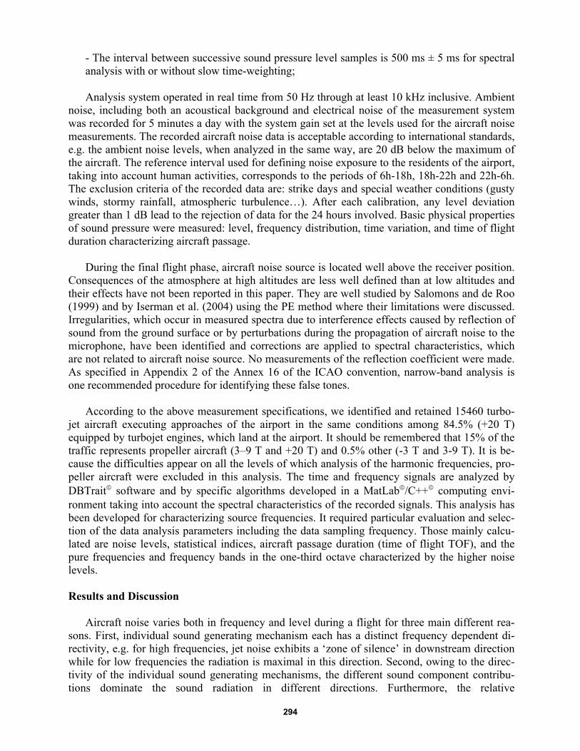
The time-resolution depends on the time-window gM(m), and it is lower in SWV than in WV. Moreover, SWV does not satisfy the marginal conditions. To reduce the cross-terms satisfying the marginal conditions, a larger class of time-frequency distributions, such as the Choi-Williams distribution, which includes the Wigner-Ville as a special case, could be suggested. When the signal is composed of several components interference occurs between their time-frequency pat-terns due to the bilinear nature of the distribution. To reduce this effect the transform is smoothed in frequency – in our case by a Hanning window over 512 points. The software tool-box (MatLab© and C++©) has been used for aircraft-noise signal processing that offers a more informative description of signals such as the predominant frequency emitted during aircraft ap-proach. Figure 6 shows a typical time-frequency spectrum of aircraft noise measured during three approaches. It gives an illustration of a Wigner-Ville distribution used in this paper show-ing the distribution of energy in the sound across frequency.

Fig. 6: Time-frequency spectrum of three aircraft approaches.

Figure 7 reveals the two major components in ground-perceived aircraft noise: broadband noise and some tonal components. As previously mentioned, interference pattern resulting from direct and reflected noise is not considered. The amplitude of the broadband noise in third-octave bands is determined based on the aver-age energy that remains in each band after removing all tonal components from that band. An automatic search of maximum levels was achieved and pure frequencies or frequency bands were made from recording spectra. Identification and counting of frequency bands were made by using specific routines developed under MatLab© and C++©. After normalization compared to the total number of sound signatures, we obtained the result shown in Figure 8 to show what the

302

third-octave bands perceived level sensor with the highest levels. The major observed bands are 630 Hz, 800 Hz, 1000 Hz, 1250 Hz and 1600 Hz, whose noise levels are the highest. The third-octave bands 1.25 kHz and 1.6 kHz are dominating. Their origin could be either the airframe of the aircraft (fuselage, wing, drift, landing gear and high lift devices), which upon landing with an engine rpm in slow motion, may have a higher contribution from 10 dB above the noise of the engine; or engines, particularly the combustion chamber and the turbines that are emitting broadband sounds between 1500 Hz and 5000 Hz. At this stage, one cannot attribute these fre-quency bands to a defined source but to the whole (nacelle - components - engines).

Fig. 7: Cumulate noise levels (1/3-octave bands).

Fig. 8: The dominant frequency bands.

303

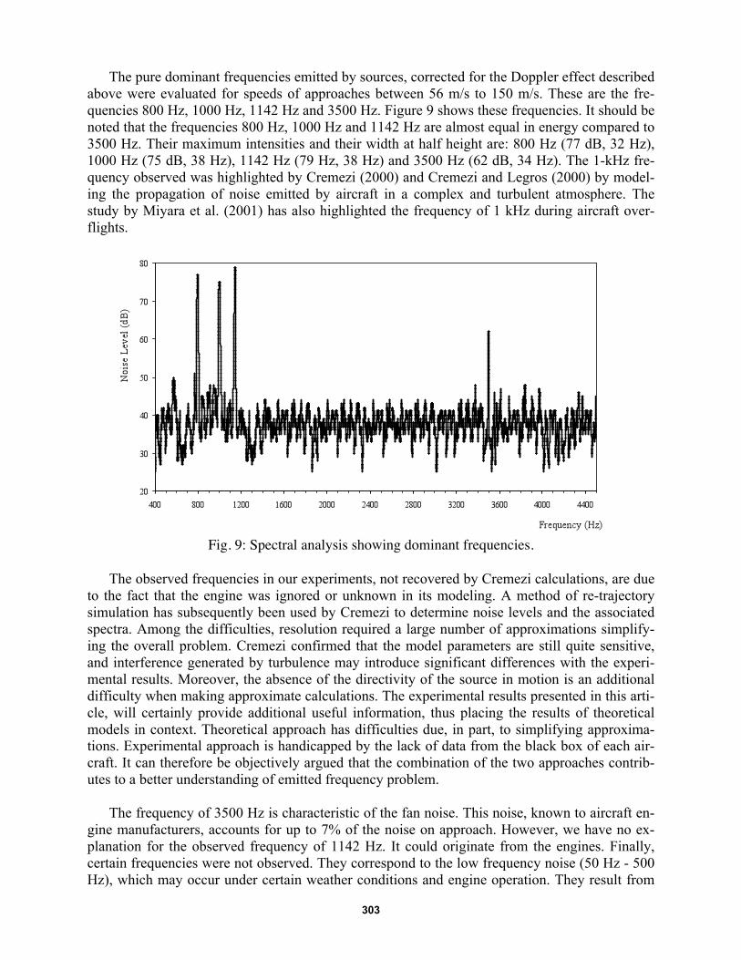
The pure dominant frequencies emitted by sources, corrected for the Doppler effect described above were evaluated for speeds of approaches between 56 m/s to 150 m/s. These are the fre-quencies 800 Hz, 1000 Hz, 1142 Hz and 3500 Hz. Figure 9 shows these frequencies. It should be noted that the frequencies 800 Hz, 1000 Hz and 1142 Hz are almost equal in energy compared to 3500 Hz. Their maximum intensities and their width at half height are: 800 Hz (77 dB, 32 Hz), 1000 Hz (75 dB, 38 Hz), 1142 Hz (79 Hz, 38 Hz) and 3500 Hz (62 dB, 34 Hz). The 1-kHz fre-quency observed was highlighted by Cremezi (2000) and Cremezi and Legros (2000) by model-ing the propagation of noise emitted by aircraft in a complex and turbulent atmosphere. The study by Miyara et al. (2001) has also highlighted the frequency of 1 kHz during aircraft over-flights.

Fig. 9: Spectral analysis showing dominant frequencies.

The observed frequencies in our experiments, not recovered by Cremezi calculations, are due to the fact that the engine was ignored or unknown in its modeling. A method of re-trajectory simulation has subsequently been used by Cremezi to determine noise levels and the associated spectra. Among the difficulties, resolution required a large number of approximations simplify-ing the overall problem. Cremezi confirmed that the model parameters are still quite sensitive, and interference generated by turbulence may introduce significant differences with the experi-mental results. Moreover, the absence of the directivity of the source in motion is an additional difficulty when making approximate calculations. The experimental results presented in this arti-cle, will certainly provide additional useful information, thus placing the results of theoretical models in context. Theoretical approach has difficulties due, in part, to simplifying approxima-tions. Experimental approach is handicapped by the lack of data from the black box of each air-craft. It can therefore be objectively argued that the combination of the two approaches contrib-utes to a better understanding of emitted frequency problem. The frequency of 3500 Hz is characteristic of the fan noise. This noise, known to aircraft en-gine manufacturers, accounts for up to 7% of the noise on approach. However, we have no ex-planation for the observed frequency of 1142 Hz. It could originate from the engines. Finally, certain frequencies were not observed. They correspond to the low frequency noise (50 Hz - 500 Hz), which may occur under certain weather conditions and engine operation. They result from

304

the mixing of hot jet at the exit reactors (severe turbulence). The frequency of 63 Hz, observed by Miyara et al. was not found in this study, due to limitations of our system of measurements at frequencies below 200 Hz. Regarding noise in the environment, it is essential to remember that the observed frequency bands 630 Hz, 800 Hz, 1000 Hz, 1250 Hz and 1600 Hz and 800 Hz fre-quency pure, 1000 Hz, 1142 Hz, and 3500 Hz, are emitted during phases of approach and are characterized by the highest noise levels. This may steer some research on the nuisance of air-craft noise around airports and assesses the relevant areas to be developed taking into account the type of aircraft and flights, while preserving the performance gained for flight safety and useful lives of the engines.

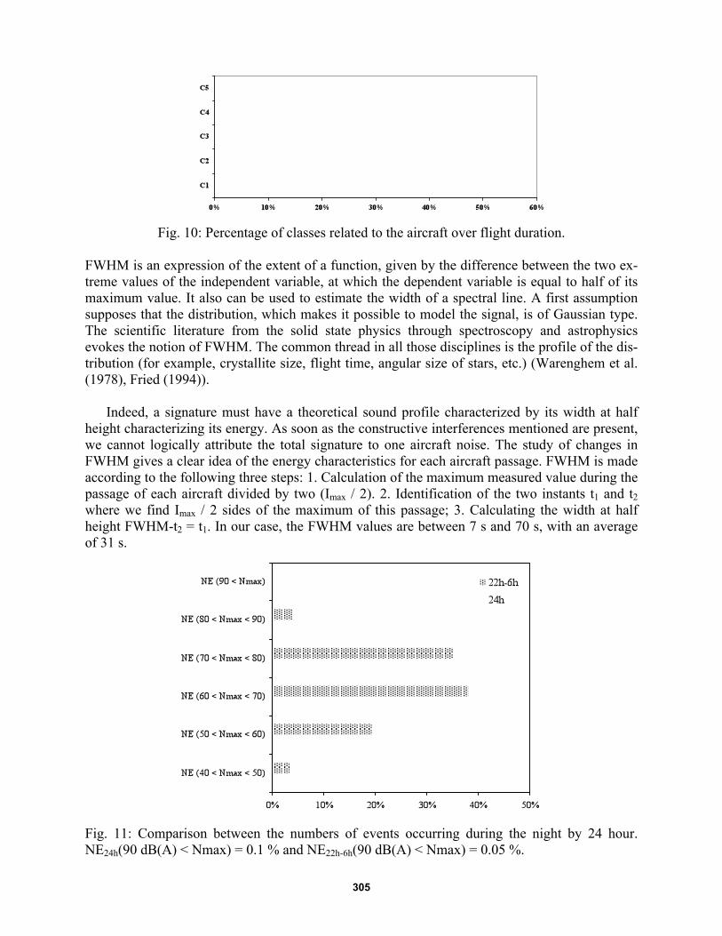
On the one hand, broadband noise arises from the combustion chamber during the combus-tion process, from the turbulence in the jet of engines and from air flow around the aircraft na-celle. On the other hand, tonal components occurring between 1000 and 7000 Hz are particularly emitted by the turbine and the compressor for the turbojet engines. In addition, the latter can be generated by flows over cavities such as the landing gear box and flows on the level of the flaps. Also, it has been shown that from time to time the tonal components do not appear in a narrow frequency region but in a large interval of the spectrum. It can occur when tonal components have very close values or when the source frequencies have undergone fast changes around an average frequency. This phenomenon is significant for aircraft manufacturers because of active and passive controls implementation. Nevertheless, it has no meaning for the psycho-acoustic community because human hearing is often unable to distinguish close frequencies. In addition, even a clear directivity towards the front of aircraft, time-frequency spectra recorded from air-craft approaches did not show discrete tones due to rotational speed of the engine axis. Aircraft Time of Flight The study of aircraft noise in the environment supposes knowledge of the relevant objectives and tools for characterizing its quality. For a long time, a lot of work has been directed towards statistical indicators (Nelson, 1987; CEC, 1999; Koppert, 2000). Many authors continue to sug-gest indicators even if Lden is nowadays considered as a reference. Literature review shows dif-fering visions which confirm the continuation of research in this field. Impact of aircraft noise around airports is often associated with the duration of exposure to noise events. Thus, analysis of the time of flight (TOF) completes those indices in the context of an overall vision, which must implicitly take into account air traffic morphology. For one-year measurements, we there-fore determined classes corresponding to the TOF, by time intervals. These classes are divided into five: 1. C1 (TOF is between 20 and 30 sec), 2. C2 (31 - 60 sec), 3. C3 (61 - 90 sec), 4. C4 (91 - 120 sec) and 5. C5 (121 - 125 sec) shown in Figure 10 which TOF varies from 20 s to 125 s for all selected flights. 88% of the TOF are between 31 and 90 sec (51.6% between 31 and 60 s; 36.3% between 61 and 90 s). Raney and Cawthorn (1979) established an average TOF of 60 s, and Cremezi (2000) gave an average time between 40 and 50 s. Noise levels represented by the index SEL ranged from 54 dB (A) to 109.3 dB (A). 2% of approaches (SEL varying from 62 to 101 dB (A)) have not been accepted (over flight, passages of light vehicles, heavy agricultural or construction sites …) for social and economic activities around the airport. We calculated, in turn, the full width at half maximum FWHM as an index of each aircraft acoustic signature to explore future opportunities allowing to progress in the field of the indica-tors, which objectify the environmental impact of aircraft noise around airports. Thus,

305

Fig. 10: Percentage of classes related to the aircraft over flight duration.

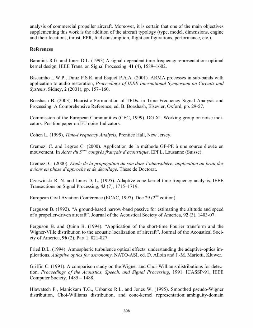
FWHM is an expression of the extent of a function, given by the difference between the two ex-treme values of the independent variable, at which the dependent variable is equal to half of its maximum value. It also can be used to estimate the width of a spectral line. A first assumption supposes that the distribution, which makes it possible to model the signal, is of Gaussian type. The scientific literature from the solid state physics through spectroscopy and astrophysics evokes the notion of FWHM. The common thread in all those disciplines is the profile of the dis-tribution (for example, crystallite size, flight time, angular size of stars, etc.) (Warenghem et al. (1978), Fried (1994)). Indeed, a signature must have a theoretical sound profile characterized by its width at half height characterizing its energy. As soon as the constructive interferences mentioned are present, we cannot logically attribute the total signature to one aircraft noise. The study of changes in FWHM gives a clear idea of the energy characteristics for each aircraft passage. FWHM is made according to the following three steps: 1. Calculation of the maximum measured value during the passage of each aircraft divided by two (Imax / 2). 2. Identification of the two instants t1 and t2 where we find Imax / 2 sides of the maximum of this passage; 3. Calculating the width at half height FWHM-t2 = t1. In our case, the FWHM values are between 7 s and 70 s, with an average of 31 s.

Fig. 11: Comparison between the numbers of events occurring during the night by 24 hour. NE24h(90 dB(A) < Nmax) = 0.1 % and NE22h-6h(90 dB(A) < Nmax) = 0.05 %.

306

We also analyzed the following noise indices: Leq24h, Leq6h-18h, Leq18h-22h, Leq22h-6h, LDN, LDEN, SEL, and DEN LDNL depending on the day of the week. Three groups can be distin-guished: SEL whose levels are distributed around 100 dB (A), [DEN, LDNL] around 75 dB (A) and the group [Leq24h, Leq6h-18h, Leq18h-22h, Leq22h-6h, LDN, LDEN] whose levels are between 48 and 56 dB (A). The problem is to define the upper and lower limits for each of the indices and their ability to objectify the impact of air traffic on the environment. This result confirms that we must guide the analysis of indices to study each event such as the aircraft passage. It would be necessary to introduce the type of aircraft and flights. Thus, for night flights (22h-6h), we have performed an analysis of events (maximum levels produced by the passage of each aircraft) rep-resenting 15.1% of the total number of aircraft because people neighboring the airport are sensi-tive to those flights. The effect on health has already been demonstrated in the past. In this paper, we classified noise levels and we compared them to their corresponding period of 24 h. Events producing maximum noise levels belonging to a specified interval were recorded. Figure 11 shows the percentages of the numbers of events (NE). 0.1% of events whose maximum levels are above 90 dB (A) for periods of 24h and 0.05% for periods of night (respectively 8 and 1 aircraft) are not represented. The analysis shows that the majority of NE is situated between 50 and 80 dB(A). Almost every percentages of night are slightly higher than those obtained during the 24 h except for those, which are located in the interval 60-70 dB(A). The differences vary from 1 to 3%. In conclusion, we have fewer aircraft at night but that generate maximum levels comparable to those of 24 h or even in days. This finding could lead policy makers, managers of airports, air-lines … to recommend that pilots use approach procedures, which generate less noise, in particu-lar, at night. To broaden the scope of this analysis, we reviewed in the next paragraph quiet and noisy pe-riods. In addition, before examining the quiet and noisy periods, we made an initial separation according to the time and number of aircraft on approach. The traffic distribution providing addi-tional information useful in interpreting the results is: 61% of aircraft approaching between 6h and 18h, 24% between 18h and 22h, and 15% between 22h and 6h. This traffic distribution cer-tainly has an effect on the analysis of the noisy and quiet times of the day. The analysis of the noisiest and quietest periods was carried out every 30 minutes; they are defined in the following manner: first, we define a cumulative duration of one minute corresponding to the time step and calculate levels minute by minute. Then, for each 30 minutes the highest and lowest values are compared to background noise. We show in Fig. 12 periods and percentages corresponding to the lowest observed levels. 60% of the lowest levels are achieved during the period between 0h and 2h, which is followed by the 2h-4h period (26%), then 14% for 4h-6h and 22h-0h periods.

Fig. 12: The quietest periods. Fig. 13: The noisiest periods.

307

The silent period is between 0h-2h. The average difference between the levels recorded dur-ing this period and L95 (~ 41 dB (A)) is 1.7 dB (A). In addition, the period 14h-16h represents 49% of the highest noise levels of the day (Figure 13). It is followed by the period 10h-12h (25%), and then by periods 8h-10h and 16h-18h (respectively 15% and 11%). The average dif-ference between the levels recorded during the noisiest and L95 is 36.8 dB (A). This gap is almost 22 times higher than for the quietest period.

The average noise level of the most silent period is 45 dB (A) and 77.3 dB (A) for the most noisy. Periods 6h-8h, 12h-14h and 18h-22h do not appear, according to the definition, among the noisiest or the quietest period of a day. These periods are characterized by intermediate noise levels between the two provided previously. When one counts the number of hours correspond-ing to the quieter periods (S), intermediate (I), and most noisy (B), there is an equi-partition, i.e. 8 hours for each type of period. Clearly, in terms of sound annoyances, periods (I), or a part, might be confused with periods (B). It is known that the impacted ground surface decreases with the noise level. Thus, it is essential that this information be considered in the analysis of events as it gives objective knowledge of a sound situation. Conclusion Time-frequency analysis (Wigner-Ville distribution) has been applied to process experimen-tal data. Computing and interpreting time-frequency distributions of aircraft noise is quite a long operation. A procedure was tested using one-dimensional variables. This work is directed to-wards the search of the dominant pure frequencies and the aircraft passage times when approach-ing the Saint-Exupéry Lyon International Airport. This research provides aircraft manufacturers with frequencies emitted during approaches, which should be treated at the source. It also allows the diagnosis of frequencies responsible for the noise annoyances surrounding the airport. Measurements of aircraft noise in the vicinity of the airport were conducted during one year. They served as a reference year because of changes in the airport infrastructure project including the two new runways, planned for 2015, renewal of fleets conditioned by the evolution of aircraft certification and regulation, etc. A geometric study of frequency emission according to the an-gles and indicated aircraft speeds on approach has been finalized. Doppler corrections have been made and diagnosis of the effects of destructive interference examined. Dominant pure frequen-cies were observed and their analysis reveals an agreement with theoretical works. Their origin could come from the airframe of the aircraft (fuselage, wing, drift, landing gear and high lift de-vices), which upon landing with an engine rpm at idle up to 55% for some aircraft can have a higher contribution from 10 dB above the noise of the engine. Next, we analyzed the noise levels over time and aircraft passage times. We identified the quietest and noisiest periods. The relative sensitivity of acoustical indices confirms the need for further research including the morphology of air traffic, the type of aircraft and flight configurations. One must take ac-count fleet renewal, introduction of engines and cells’ breakthrough technologies, etc. We must focus more on analysis of individual temporal events considering the impacted ground surfaces. This is a result of environmental situations conditioned by the emergence of new aviation tech-nologies. Experimental results presented in this paper could validate and extend calculation methods. They provide additional useful information placing the results of theoretical models in context because of strong approximations for calculation needs. This work has been performed for turbojet aircraft with the aim of analyzing the frequency characterized by higher levels. Nev-ertheless, it is clear that additional research is needed to achieve this goal by performing noise

308

analysis of commercial propeller aircraft. Moreover, it is certain that one of the main objectives supplementing this work is the addition of the aircraft typology (type, model, dimensions, engine and their locations, thrust, EPR, fuel consumption, flight configurations, performance, etc.). References Baraniuk R.G. and Jones D.L. (1993) A signal-dependent time-frequency representation: optimal kernel design. IEEE Trans. on Signal Processing, 41 (4), 1589–1602. Biscainho L.W.P., Diniz P.S.R. and Esquef P.A.A. (2001). ARMA processes in sub-bands with application to audio restoration, Proceedings of IEEE International Symposium on Circuits and Systems, Sidney, 2 (2001), pp. 157–160. Boashash B. (2003). Heuristic Formulation of TFDs. in Time Frequency Signal Analysis and Processing: A Comprehensive Reference, ed. B. Boashash, Elsevier, Oxford, pp. 29-57. Commission of the European Communities (CEC, 1999). DG XI. Working group on noise indi-cators. Position paper on EU noise Indicators. Cohen L. (1995), Time-Frequency Analysis, Prentice Hall, New Jersey. Cremezi C. and Legros C. (2000). Application de la méthode GF-PE à une source élevée en mouvement. In Actes du 5ème congrès français d’acoustique, EPFL, Lausanne (Suisse). Cremezi C. (2000). Etude de la propagation du son dans l’atmosphère: application au bruit des avions en phase d’approche et de décollage. Thèse de Doctorat. Czerwinski R. N. and Jones D. L. (1995). Adaptive cone-kernel time-frequency analysis. IEEE Transactions on Signal Processing, 43 (7), 1715–1719. European Civil Aviation Conference (ECAC, 1997). Doc 29 (2nd edition). Ferguson B. (1992). “A ground-based narrow-band passive for estimating the altitude and speed of a propeller-driven aircraft”. Journal of the Acoustical Society of America, 92 (3), 1403-07. Ferguson B. and Quinn B. (1994). “Application of the short-time Fourier transform and the Wigner-Ville distribution to the acoustic localization of aircraft”. Journal of the Acoustical Soci-ety of America, 96 (2), Part 1, 821-827. Fried D.L. (1994). Atmospheric turbulence optical effects: understanding the adaptive-optics im-plications. Adaptive optics for astronomy. NATO-ASI, ed. D. Alloin and J.-M. Mariotti, Kluwer. Griffin C. (1991). A comparison study on the Wigner and Choi-Williams distributions for detec-tion. Proceedings of the Acoustics, Speech, and Signal Processing, 1991. ICASSP-91, IEEE Computer Society. 1485 – 1488. Hlawatsch F., Manickam T.G., Urbanke R.L. and Jones W. (1995). Smoothed pseudo-Wigner distribution, Choi-Williams distribution, and cone-kernel representation: ambiguity-domain

309

analysis and experimental comparison Source. Signal Processing. 43 (2), 149 – 168. Elsevier North-Holland, Inc. Hubbard H. H. (1994). Aeroacoustics of flight vehicles, vol. 1: Noise sources, Acoustical society of America, New York Hunter, C.A. and Thomas, R.H. (2003). Development of a Jet Noise Prediction Method for In-stalled Jet Configurations. 9th

AIAA/CEAS Conf. and exhibit, 12-14. Hilton Head, SC. ICAO (1988). “Recommended method for the calculation of the noise level contours in the vicin-ity of airports”. Circular 205-AN/1/25. International Civil Aviation Organization. Montreal, Canada. ICAO (1993). “Aircraft Noise”. Annex 16 to the Convention on International Civil Aviation. In-ternational Civil Aviation Organization. Montreal, Canada. ICAO (2004). Environment protection. Vol. 1: aircraft noise – specifications for aircarft noise certification, noise monitoring, and noise exposure units for landuse planning. Available on http://www.icao.int/ Iserman, U., Boguhn, O., Henkel, C., Kowalski, T. Schmid, R. (2004) “Simulationsverfahren zur Fluglärmprognose”, Ablschlusspräsentation Project “Leiser Flugverkehr”. Köln-Porz, March 2004. Jones D.L. and Baranuik (1994). A Simple Scheme for Adapting Time-Frequency Representa-tions. IEEE Trans. Sig. Proc., 42, 3530-3535. Jones D.L. and Baraniuk R.G. (1995). An adaptive optimal kernel time-frequency representation. IEEE Transactions on Signal Processing, 43 (10), 2361–2371. Julliard J. (2003). Bruit des turboréacteurs et dispositifs réducteurs. Dans S. Khardi, Journée Spécialisée « Réduction des bruits des avions commerciaux au voisinage des aéroports civils. Problématique, enjeux et perspectives ». Actes n°88, 53 – 63. Kannepalli, C., Kenzakowski, D. C. and Dash, S.M. (2003). Evaluation Of Some Recent Jet Noise Reduction Concepts. Paper No. AIAA-2003-3313, 9th AIAA/CEAS Aeroacoustics Confer-ence & Exhibit, Hilton Head, SC. Kenzakowski, D.C., Papp, J.L., and Dash, S.M. (2002). Modeling Turbulence Anisotropy For Jet Noise Prediction. Paper No. AIAA-2002-0076, 40th AIAA Aerospace Sciences Meeting and Ex-hibit, Reno, NV, 14-17. Koppert A.J. (2000). Fact sheets on different European noise calculation methods (RLD). Kwok H.K. and Jones D.L. (2000) .Improved Instantaneous Frequency Estimation Using an Ad-aptive Short-Time Fourier Transform. IEEE Trans. Sig. Proc., 48 (10), 2964-2972. Li M., 1997. Experimental research for processing of Choi-Williams distributionand Bessel dis-tribution. Proceedings of International Conference on Information, Communications and Signal Processing ICICS. Volume 3, 1593 – 1597.

310

Lo, K.W.; Perry, S.W. and Ferguson, B.G. (1999). An image processing approach for aircraft flight parameter estimation using the acoustical Lloydapos; mirror effect. Signal Processing and Its Applications. ISSPA. Proceedings of the Fifth International Symposium on Digital Object Identifier. Vol. 2, pp. 503-506. Michel U., Barsikow B., Helbig J., Hellmig M. and Schüttpelz M. (1998). “Flyover noise meas-urements on landing aircraft with a microphone array”, AIAA Paper 98-2336. Miyara C., Cabanellas S., Mosconi P., Pasch V., Yanitelli M., Rall J.C. and Vasquez J. (2001). The acoustical geometry of aircraft overflights. International Congress and Exhibition on Noise Control Engineering. Hague (NL), 27 – 30. Nelson P.M. (1987). Transportation Noise Reference Book. Part. Aircraft Noise, Butterworth & Co. Ltd. Oishi T. and Nakamura Y. (2000). Research on exhaust jet noise reduction technology. Ishika-wajima-Harima Giho. 40 (2), 65-67. ISSN 0578-7904. CODEN ISHGAV. Oppenheim AV and Schafer RW (1989) Discrete-time signal processing, Prentice-Hall, Engle-wood Cliffs, NJ. Orfanidis S.J. (1988). Optimum signal processing. 2nd ed., McGraw-Hill. Papandreou, A. and Boudreaux-Bertels, G.F. (1993). Generalization of the Choi-Williams Dis-tribution and the Butterworth Distribution for Time-Frequency Analysis. IEEE Transactions on Signal Processing. 41 (1), 463 – 498. Raney, J.P. and Cawthorn J.M. (1979). Aircraft noise. Handbook of noise control. ed. C.M. Har-ris. McGraw-Hill. Salomons E. and de Roo F. (1997). “Modelling of Aircraft Noise Propagation”, Proceedings of NAG symposium. NAG Journaal 147, 31-44. Schulten J.B.H.M. (1997). Computation of aircraft noise propagation trough the atmospheric boundary layer. National Aerospace Laboratory NLR, Amsterdam, The Netherlands. Smith M.J.T. (1989). Aircraft noise, Cambridge Univ. Press, Cambridge, UK. Warenghem M., Cuvelier P. and Billard J. (1978). Plane uniformly heterogeneous wave diffrac-tion. J. Opt. 9, 79-82. Zaporozhets O. I. and Khardi S. (2004). Optimisation of aircraft trajectories as a basis for noise abatement procedures around the airports. Theoretical considerations and acoustic applications. Les collections de l’INRETS. Rapport INRETS n° 257. 97 pages. Zaporozhets O. I., Tokarev V. I. (1998). Predicting Flight Procedures for Minimum Noise Im-pact. Applied Acoustics, 55 (2), 129–143.