An Exact and Efficient Algorithm for the Constrained Dynamic

Operator Staffing Problem for Call Centers

Atul Bhandari∗ Alan Scheller-Wolf Mor Harchol-Balter

December 17, 2005

Abstract

As a result of competition, call centers face increasing pressure to reduce costs while main-

taining an acceptable level of customer service, which to a large extent entails reducing the time

customers spend waiting for service. Pursuant to this, call center managers often face stochastic

constrained optimization problems with the objective of minimizing cost, subject to certain cus-

tomer waiting time constraints. Complicating this problem is the fact that in practice, customer

arrival rates to call centers are often time-varying.

In order to cost-effectively satisfy their service level goals in the face of this uncertainty, call

centers may employ a certain number of permanent operators who always provide service, and

a certain number of temporary operators who provide service only when the call center is busy,

i.e.when the number of customers in system increases beyond a threshold level. This gives the

call center manager the flexibility of dynamically adjusting the number of operators providing

service (and thus the resources or costs dedicated) in response to the time-varying arrival rate.

The Constrained Dynamic Operator Staffing (CDOS) problem involves determining the

values for the number of permanent operators, the number of temporary operators, and the

threshold value(s) that minimize time-average hiring and opportunity cost, subject to service

level constraints. Currently, the only exact solution method for this problem is enumeration,

which is often computationally intractable. We provide an exact and efficient solution method,

the Modified-Balance-Equations-Disjunctive-Constraints (MBEDC) algorithm, for this problem

resulting in a Mixed Integer Program formulation. Using our algorithm, we solve diverse in-

stances of the CDOS problem, generating managerial insights regarding the effects of temporary

operators and service level constraints.

∗Corresponding author; email: atulb@cmu.edu

1

1 Introduction

For many organizations in the service industry, call center quality is a critical component of customer

loyalty and hence revenue generation. Call centers offer a product or service through telephone lines

(or the Internet) to customers who in turn have expectations regarding the quality of the service

they will receive. These expectations can be distinguished into two categories: time spent waiting

for an operator to provide service, and the human-interaction with the operator. To improve the

human-interaction element of service, call centers provide training to their staff or operators. To

reduce customer waiting time, call centers can hire more (or better) operators. But, while the

need to meet service level goals is critical, call centers also face increasing pressure to reduce costs.

Thus, call center managers are concerned with increasing the efficiency of call centers (Gans et al.,

2003) - improving service quality while controlling costs. One way to achieve staffing efficiency is

to correctly schedule operators: Over-staffing leads to unnecessary costs, while under-staffing will

result in dissatisfied customers and possibly a loss of business/revenue (Brigandi et al., 1994).

The problem of long-term operator staffing to meet time-varying demand is well studied, refer

for example to Hall (1991), Jennings et al. (1996), Gans et al. (2003), and the references therein.

Typically for this problem, the time horizon is divided into smaller periods and deterministic

forecasts for the customer arrival rates for each period are used to determine the respective staffing

levels. However, it has been observed in practice that the customer arrival rate may itself be

random within a period, and that it thus may be risky to ignore arrival rate uncertainties (Gans

et al., 2003). Specifically, if the number of operators (determined from the forecast of the average

arrival rate) is fixed for each period, the following two scenarios may occur: (i) the arrival rate

may be lower than expected resulting in operators being idle and hence, unnecessary costs, or (ii)

the arrival rate may be higher than expected resulting in long waiting times and hence, inability

to meet the call center service level goals.

One method of accommodating time-varying demand rate is numerical, assuming the (time-

varying) demand rate is known. Yoo (1996) and Ingolfsson et al. (2002) investigate such methods,

numerically solving the Chapman-Kolmogorov forward equations for Mt/M/Nt systems to calcu-

late the associated transient system behavior. A second method is to model a random arrival rate

switching between states with different arrival rates, with switching times having certain distribu-

2

tions (Nain and Nunez-Queija, 2001). In either situation, and in fact even under stationary arrival

rates, call centers may benefit from flexible staffing - the ability to dynamically adjust staffing levels

with traffic. Such flexibility may be attained by utilizing temporary operators, in addition to the

permanent operators who are always available to provide service. The temporary operators may

be either supervisors/managers or other operators who are on call (Whitt, 1999; Jongbloed and

Koole, 2001); these temporary operators provide service at the call center manager’s discretion.

Within the context of this paper we define the Constrained Dynamic Operator Staffing (CDOS)

problem as follows. It involves determining the number of permanent operators to hire, the number

of temporary operators to hire, and the number of temporary operators to use at every state of the

call center queuing model, in order to minimize the time-average hiring and opportunity cost subject

to service level constraints. Typical examples of service level constraints are: (i) probability of delay

is below q, (ii) average waiting time is less than t time units, (iii) average number of customers in

queue is less than p, etc. Such an objective, and similar constraints, are proposed in Jongbloed and

Koole (2001) also, but they consider the problem of providing stochastic guarantees for constraint

satisfaction by considering percentile levels of an arrival-rate random variable. Another difference

is that they call upon the temporary operators when the realized non-varying arrival-rate in a

period is higher than expected, while in our model the arrival rate, and hence the optimal number

of operators may change stochastically.

For simplicity, we restrict our attention to simple threshold policies for utilizing the temporary

operators (which may in general be sub-optimal). Threshold policies specify two critical values:

(i) If the number of jobs in system reaches the higher critical value, the call center manager asks

the temporary operators to provide service. (ii) When the number of jobs in system falls to the

lower threshold value and all temporary operators are idle, the temporary operators stop providing

service. This restriction to threshold policies is similar to, and shares common motivation with,

the restriction to base-stock policies in complex inventory environments. Examples are models for

spare parts networks (Wong et al., 2006), perishable items (Deniz et al., 2005; and the references

therein), and supply chains featuring multiple supply modes (Veeraraghavan and Scheller-Wolf,

2005).

Under suitable assumptions for the arrival process and service time distributions, the CDOS

problem can be modeled as a Markov Decision Process (MDP) with probabilistic constraints (Put-

3

erman, 1994). For MDPs without constraints, there exist efficient solution algorithms (Puterman,

1994; Bertsekas, 1995; Porteus, 2002), namely: policy iteration, value iteration and linear pro-

gramming. However, if there are probabilistic constraints, we are not aware of any straightforward

implementation of policy iteration or value iteration. The existing linear programming method can

model constraints, but typically results in an optimal randomized policy (Puterman, 1994). This

means that in some states it may be optimal to use a chance mechanism to determine the course of

action. This can be a drawback, as often managers are interested in optimal non-randomized poli-

cies. Currently, the only exact solution method for obtaining the optimal non-randomized policy

to the CDOS problem is enumeration, which is typically computationally intractable for problems

of any size.

Our contribution in this paper is the explicit modeling of the CDOS problem for which we

develop an exact and efficient algorithm (the Modified-Balance-Equations-Disjunctive-Constraints,

MBEDC, algorithm) for non-randomized policies, resulting in a Mixed Integer Program (MIP)

formulation (Nemhauser and Wolsey, 1988). Our paper is different from the existing literature as

we take into account the time-varying customer arrival rate, allow temporary operators, consider

explicit service level constraints, and provide an exact and efficient solution method that gives the

optimal number of permanent and temporary operators as well as answers the question of when

the temporary operators should be called in. Using our algorithm, we solve diverse instances of

the CDOS problem, demonstrating the economic effects of temporary operators and service level

constraints.

The remainder of the paper is organized as follows. We provide the problem description for

the Constrained Dynamic Operator Staffing (CDOS) problem in Section 2. Section 3 discusses

the existing Linear Program (LP) method that results in an optimal randomized solution for the

CDOS problem. We develop the Modified-Balance-Equations-Disjunctive-Constraints (MBEDC)

algorithm to obtain the optimal non-randomized solution for the CDOS problem in Section 4. Com-

putational results featuring economic insights for managers and computational speed are discussed

in Section 5. We discuss extensions of the CDOS model in Section 6. Finally, Section 7 presents

conclusions and directions for future work.

4

2 CDOS Problem Description

We model a call center with both permanent and temporary operators (supervisors or stand-by

operators). We assume the permanent operators are always available to provide service, but the

call center manager decides when to use the temporary operators. We define the system state as

the number of jobs in system, and initially we assume that the maximum number of jobs in the

system is finite, Nt, which results in a finite state space. (We address models with infinite state

space in Section 6.) At each state, the optimal number of temporary operators to be used may be

different; however, such policies are more complicated to implement than simple threshold policies.

Therefore we restrict our focus to threshold policies for temporary operators.

In a threshold policy, the call center manager asks the temporary operators to provide service

when the number of jobs in system increases to a threshold value. The temporary operators

continue to be available until the number of jobs in system reaches a second threshold value, and

all temporary operators are idle. When this happens, we assume the temporary operators stop

providing service en masse and return to stand-by mode. (We can also model the case where

the temporary operators return to stand-by mode individually, as they become idle.) We also

assume that if a temporary operator is providing service to a customer, the customer will not

be transferred to a permanent operator if one becomes idle. We make this assumption only for

practical considerations, as a customer may be dissatisfied if the operator is changed during service.

Finally, we assume that when a customer arrives and both a permanent operator and a temporary

operator are idle, the customer is assigned to the permanent operator. We can model and solve the

cases when any of these assumptions are relaxed.

We seek to minimize the time-average hiring and opportunity cost subject to service level

constraints. The following subsections provide details of the cost structure and of the service level

constraints that we consider.

2.1 Costs and Decision Parameters

Let the number of permanent operators hired be x and the number of temporary operators hired

to be on call be y. The time-average cost of hiring each permanent (temporary) operator is p1

(p2), with p2 < p1; it is cheaper to hire temporary operators on stand-by than to have full-time

5

permanent operators. (The p2 ≥ p1 case can likewise be analyzed, but results in y = 0.) Initially,

only the permanent operators provide service and the call center behaves as a x-server central queue

system. Let the two threshold values for changing the number of operators be denoted by n and m

(n > m). Thus when the number of jobs in system reaches n, all y temporary operators are asked

to provide service and the call center behaves as a (x + y)-server central queue system (permanent

and temporary operators may have different service rates as is explained in Section 2.2). Once all

y temporary operators are idle and the number of jobs in system is at or below m, the temporary

operators return to stand-by mode. There may be an additive cost of p3 per serving temporary

operator, incurred only when a temporary operator is providing service. In the case of a supervisor

acting as a temporary operator, p3 can be considered as a penalty cost as the supervisor delays her

original work in order to provide service.

Note that once the temporary operators start providing service, the number of jobs in system

can be less than x but one or more temporary operators may still be providing service, as calls are

not transferred during service. Thus, we need to keep track of the number of temporary operators

actually providing service, and not just available, at each state of the system because of the marginal

cost p3. In this paper we assume m to be fixed at x for simplicity, but in general m can also be a

decision variable.

In addition to the operator hiring costs, there may also be opportunity costs related to the

service level goals. We define d as the one-time cost incurred if a customer experiences positive

delay, and w as the opportunity cost per unit time, incurred for each customer waiting in queue.

We include these costs in our model, as traditionally service level goals in call center optimization

problems have been modeled as opportunity costs rather than service level constraints (example:

Andrews and Parsons, 1993). Modeling service level goals as constraints, while more accurate (d

and w are usually estimates), makes the problem more difficult to solve. We discuss solution issues

in Section 3.

2.2 Arrival Process and Service Time Models

We use a two-state Markov Modulated Poisson Process (MMPP) to represent the time-varying

customer arrival process. For details on 2-state MMPP arrival process, refer to Nain and Nunez-

Queija (2001). When the state of the system is i, the customer arrival process transitions between

6

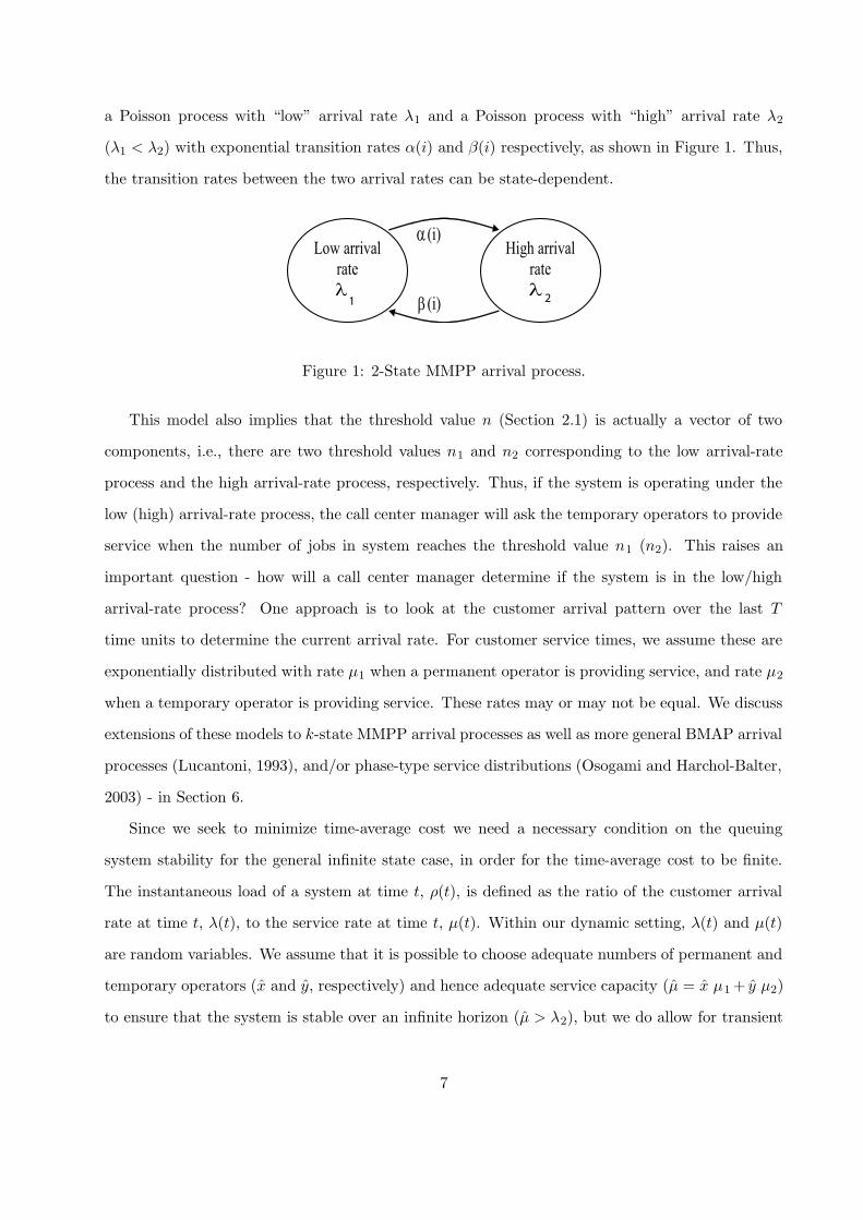
a Poisson process with “low” arrival rate λ1 and a Poisson process with “high” arrival rate λ2

(λ1 < λ2) with exponential transition rates α(i) and β(i) respectively, as shown in Figure 1. Thus,

the transition rates between the two arrival rates can be state-dependent.

Low arrival

rate

λ

High arrival

rate

λ

(i)

(i)

α

β1 2

Figure 1: 2-State MMPP arrival process.

This model also implies that the threshold value n (Section 2.1) is actually a vector of two

components, i.e., there are two threshold values n1 and n2 corresponding to the low arrival-rate

process and the high arrival-rate process, respectively. Thus, if the system is operating under the

low (high) arrival-rate process, the call center manager will ask the temporary operators to provide

service when the number of jobs in system reaches the threshold value n1 (n2). This raises an

important question - how will a call center manager determine if the system is in the low/high

arrival-rate process? One approach is to look at the customer arrival pattern over the last T

time units to determine the current arrival rate. For customer service times, we assume these are

exponentially distributed with rate µ1 when a permanent operator is providing service, and rate µ2

when a temporary operator is providing service. These rates may or may not be equal. We discuss

extensions of these models to k-state MMPP arrival processes as well as more general BMAP arrival

processes (Lucantoni, 1993), and/or phase-type service distributions (Osogami and Harchol-Balter,

2003) - in Section 6.

Since we seek to minimize time-average cost we need a necessary condition on the queuing

system stability for the general infinite state case, in order for the time-average cost to be finite.

The instantaneous load of a system at time t, ρ(t), is defined as the ratio of the customer arrival

rate at time t, λ(t), to the service rate at time t, µ(t). Within our dynamic setting, λ(t) and µ(t)

are random variables. We assume that it is possible to choose adequate numbers of permanent and

temporary operators (x and y, respectively) and hence adequate service capacity (µ = x µ1 + y µ2)

to ensure that the system is stable over an infinite horizon (µ > λ2), but we do allow for transient

7

overload; ρ(t) > 1 is permitted for some but not all t.

2.3 CDOS Problem as a Markov Decision Process with Constraints

An important result of our model assumptions is that once we fix the number of permanent op-

erators, x, number of temporary operators y, and the threshold values n1 and n2, the call center

system can be represented by a single Markov chain. Thus, the CDOS problem can be equivalently

interpreted as a problem of selecting the optimal Markov chain, or the optimal combination of the

four parameter values. Therefore, for fixed values of x and y the CDOS problem without any service

level constraints (only minimizing the time-average hiring and opportunity cost) can be represented

as a Markov Decision Process (MDP) and an average reward criterion (Puterman, 1994) with n1

and n2 as the decision parameters. We discuss the action choices for this MDP in this Section, and

defer the discussion on rewards (costs in the case of the CDOS problem) and transition rates to

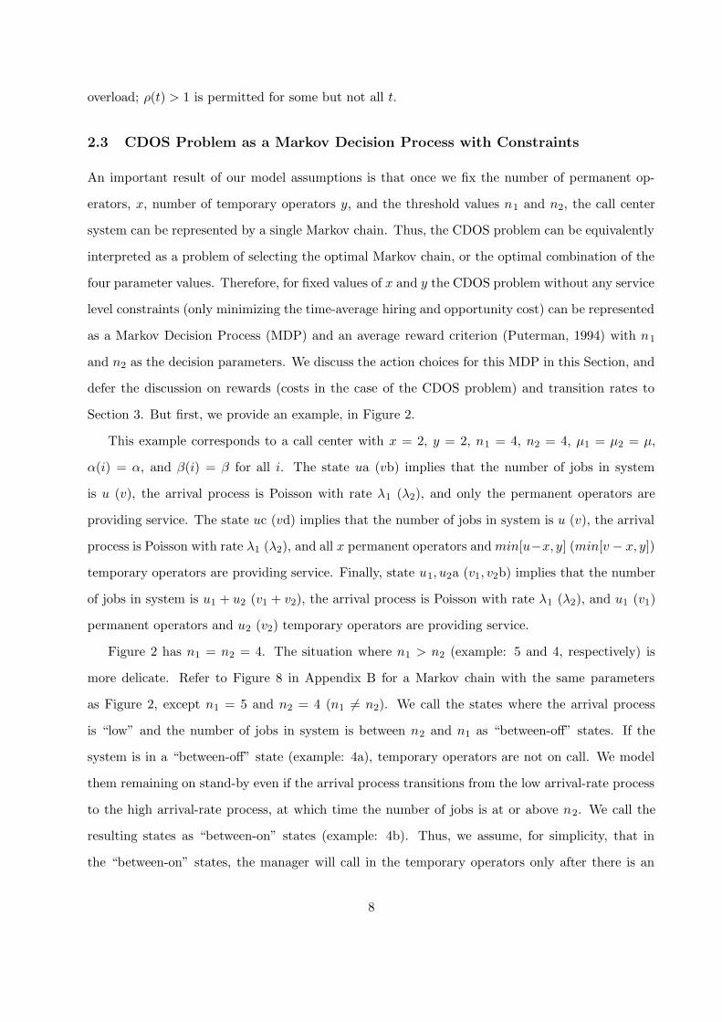
Section 3. But first, we provide an example, in Figure 2.

This example corresponds to a call center with x = 2, y = 2, n1 = 4, n2 = 4, µ1 = µ2 = µ,

α(i) = α, and β(i) = β for all i. The state ua (vb) implies that the number of jobs in system

is u (v), the arrival process is Poisson with rate λ1 (λ2), and only the permanent operators are

providing service. The state uc (vd) implies that the number of jobs in system is u (v), the arrival

process is Poisson with rate λ1 (λ2), and all x permanent operators and min[u−x, y] (min[v − x, y])

temporary operators are providing service. Finally, state u1, u2a (v1, v2b) implies that the number

of jobs in system is u1 + u2 (v1 + v2), the arrival process is Poisson with rate λ1 (λ2), and u1 (v1)

permanent operators and u2 (v2) temporary operators are providing service.

Figure 2 has n1 = n2 = 4. The situation where n1 > n2 (example: 5 and 4, respectively) is

more delicate. Refer to Figure 8 in Appendix B for a Markov chain with the same parameters

as Figure 2, except n1 = 5 and n2 = 4 (n1 6= n2). We call the states where the arrival process

is “low” and the number of jobs in system is between n2 and n1 as “between-off” states. If the

system is in a “between-off” state (example: 4a), temporary operators are not on call. We model

them remaining on stand-by even if the arrival process transitions from the low arrival-rate process

to the high arrival-rate process, at which time the number of jobs is at or above n2. We call the

resulting states as “between-on” states (example: 4b). Thus, we assume, for simplicity, that in

the “between-on” states, the manager will call in the temporary operators only after there is an

8

2µ

4µ

µ λ

λ

α

β

a

b

1

2

Permanent only

Permanent and temporary

Temporary operators return to

stand-by if all become idle

b

a

Figure 2: CDOS problem - Markov chain representation when x = 2, y = 2, n1 = n2 = 4, µ1 = µ2 =

µ, α(i) = α, β(i) = β,Nt = 6.

arrival1. We model the situation where n2 > n1 similarly.

The action state space for the MDP can be best explained by referring to Figure 2. At each

state ua (vb), there are two action choices: (i) Ask the temporary operators to help if there is an

arrival (a1). (ii) Continue without their help (a2). There is only one pre-determined action choice

(all operators are available) for each of the remaining states (uc, vd, u1, u2a, and v1, v2b). If we

select action a1 in state ua (vb) and there is an arrival (u = v = 3 in Figure 2), the Markov chain

transitions to state [u+1]c ([v + 1]d). Alternatively, if action a2 is selected in state ua (vb) and

1We can model and solve the case where if the system enters a “between-on” state, the manager immediately calls

in the temporary operators, but this model results in a Markov chain that is significantly more complicated.

9

there is an arrival (u = v = {0, 1, 2} in Figure 2), the Markov chain transitions to state [u+1]a

([v + 1]b).

For fixed values of x and y, we can solve the MDP to obtain optimal threshold values of n1 and

n2 that minimize time-average cost. For the case without service level constraints, there exist three

efficient solution techniques in the literature and Puterman (1994) is an excellent reference for their

description and comparison: (i) policy iteration, (ii) value iteration, and (iii) linear programming.

Note that we need to fix the values of x and y for the problem to be a MDP, as we do not allow

there to be different values for these parameters at different states of the system, which may happen

if we allow these to be action choices also. Solving the resulting MDPs for all choices of x and

y, and then selecting values of x, y, n1 and n2 that minimize the time-average cost will yield the

optimal threshold policy.

However, the CDOS problem has service level constraints, which complicate things significantly.

We consider the following types of service level constraints: (i) probability of delay is below q (ii)

average waiting time is less than t time units, (iii) average number of customers in queue is less than

p, etc. Constraints (ii) and (iii) are related by Little’s law and hence, we only consider constraints

(i) and (iii) here. The CDOS problem is thus an MDP problem with probabilistic constraints for

fixed values of x and y. There is no straightforward implementation of policy iteration or value

iteration for such problems (Puterman, 1994), but linear programming may be applied to problems

of this form. We discuss the linear programming algorithm in the next Section.

3 Linear Programming Method and Randomized Policies

Let Sx,y be the state space of the MDP for the CDOS problem for fixed x and y, and Ax,ys be

the set of action choices in state sεSx,y. Also, we define Sx,y1 (Sx,y

2 ) ⊂ Sx,y as follows: states

corresponding to the low (high) arrival-rate process such that all operators in that state are busy

constitute the set Sx,y1 (Sx,y

2 ). Let Bx,y be the set of states in which there is at least one idle

operator (temporary operators do not count unless they are available for service). We define πs,k to

be the limiting probability that the MDP is in state s and the call center manager chooses action

k; cs,k captures any costs associated with choosing action k in state s. Also, we define nq(j) as the

number of customers in queue in state j, which is equal to the difference between the number of

10

jobs in system and the number of operators that are busy in state j, and y(j) as the number of

temporary operators providing service - actually busy and not just available - in state j. Finally,

Γs,k is the total transition rate out of state s if action k is selected and γj|s,k is the rate of transition

to state j if action k is selected in state s.

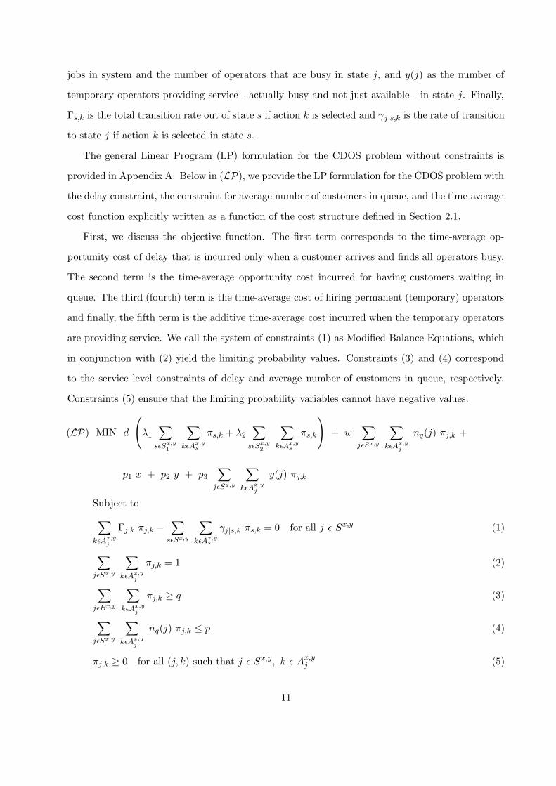
The general Linear Program (LP) formulation for the CDOS problem without constraints is

provided in Appendix A. Below in (LP), we provide the LP formulation for the CDOS problem with

the delay constraint, the constraint for average number of customers in queue, and the time-average

cost function explicitly written as a function of the cost structure defined in Section 2.1.

First, we discuss the objective function. The first term corresponds to the time-average op-

portunity cost of delay that is incurred only when a customer arrives and finds all operators busy.

The second term is the time-average opportunity cost incurred for having customers waiting in

queue. The third (fourth) term is the time-average cost of hiring permanent (temporary) operators

and finally, the fifth term is the additive time-average cost incurred when the temporary operators

are providing service. We call the system of constraints (1) as Modified-Balance-Equations, which

in conjunction with (2) yield the limiting probability values. Constraints (3) and (4) correspond

to the service level constraints of delay and average number of customers in queue, respectively.

Constraints (5) ensure that the limiting probability variables cannot have negative values.

(LP) MIN d

λ1

∑

sεSx,y1

∑

kεAx,ys

πs,k + λ2

∑

sεSx,y2

∑

kεAx,ys

πs,k

+ w∑

jεSx,y

∑

kεAx,y

j

nq(j) πj,k +

p1 x + p2 y + p3

∑

jεSx,y

∑

kεAx,y

j

y(j) πj,k

Subject to

∑

kεAx,y

j

Γj,k πj,k −∑

sεSx,y

∑

kεAx,ys

γj|s,k πs,k = 0 for all j ε Sx,y (1)

∑

jεSx,y

∑

kεAx,y

j

πj,k = 1 (2)

∑

jεBx,y

∑

kεAx,y

j

πj,k ≥ q (3)

∑

jεSx,y

∑

kεAx,y

j

nq(j) πj,k ≤ p (4)

πj,k ≥ 0 for all (j, k) such that j ε Sx,y, k ε Ax,yj (5)

11

If constraints (3) and (4) are not included, (LP) becomes a form of (LP), which yields the

optimal stationary distribution and cost. Moreover, the optimal values of n1 and n2 can then be

inferred from the limiting probability values (refer Puterman, 1994, page 393). The linear pro-

gram does not enforce non-randomized policies (randomized policies are feasible), but the vertices

of the resulting LP polyhedron have a one-to-one correspondence with non-randomized policies.

Since the optimal solution in a LP is one of the vertices of the polyhedron, the optimal policy

is non-randomized. It is important to note that one of the drawbacks of the linear programming

formulation is that the solution does not directly provide the optimal action in each state. These

have to be deduced from the limiting probability variables that are strictly positive (the limiting

probability variables have a one-to-one correspondence with state-action pairs, and in the optimal

solution only one of the limiting probability variables corresponding to a particular state will be

strictly positive). One can then solve the resulting MDPs for each combination of x and y values

to obtain the globally optimal solution.

If constraints (3) and/or (4) are included (such constraints are referred to as probabilistic

constraints in the literature), (LP) typically yields a randomized optimal policy (refer Puterman,

1994, page 406). This means that in some states it may be optimal to use a chance mechanism to

determine the course of action. An example of a randomized policy in the CDOS problem is: if

the call center system is in the low arrival-rate process, 40% of the time the manager should ask

the temporary operators to provide service if the number of jobs in system reaches ten, and 60% of

the time he should wait until the number of jobs in system reaches fifteen. This is because some of

the vertices of the new LP polyhedron will correspond to randomized policies, in particular those

vertices where at least one of the constraints (3) or (4) is binding. It is important to note that in

this case deducing the action selection in each state is more difficult, as more than one limiting

probability variable corresponding to a state will be positive: Additional steps are required to obtain

the actual randomization probabilities (solving a system of equations). While such randomized

policies may be implementable in certain MDP problems, these are, in general, harder to implement

in practice than non-randomized policies.

Currently, the only known method for obtaining an exact, non-randomized solution for MDPs

with constraints is enumeration, which is often computationally untractable. For example, in a

CDOS problem with 20 choices each for x, y, n1 and n2, enumeration will need to solve (obtain

12

limiting probability values and the objective value) 204 (=160000) Markov chains. We provide a

novel, exact, efficient approach to solve problems such as this in the next section.

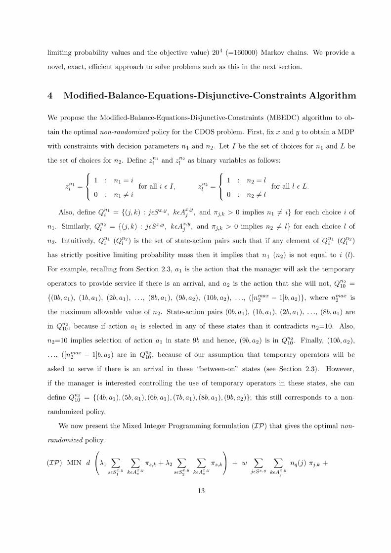
4 Modified-Balance-Equations-Disjunctive-Constraints Algorithm

We propose the Modified-Balance-Equations-Disjunctive-Constraints (MBEDC) algorithm to ob-

tain the optimal non-randomized policy for the CDOS problem. First, fix x and y to obtain a MDP

with constraints with decision parameters n1 and n2. Let I be the set of choices for n1 and L be

the set of choices for n2. Define zn1

i and zn2

l as binary variables as follows:

zn1

i =

1 : n1 = i

0 : n1 6= ifor all i ε I, zn2

l =

1 : n2 = l

0 : n2 6= lfor all l ε L.

Also, define Qn1

i = {(j, k) : jεSx,y, kεAx,yj , and πj,k > 0 implies n1 6= i} for each choice i of

n1. Similarly, Qn2

l = {(j, k) : jεSx,y, kεAx,yj , and πj,k > 0 implies n2 6= l} for each choice l of

n2. Intuitively, Qn1

i (Qn2

l ) is the set of state-action pairs such that if any element of Qn1

i (Qn2

l )

has strictly positive limiting probability mass then it implies that n1 (n2) is not equal to i (l).

For example, recalling from Section 2.3, a1 is the action that the manager will ask the temporary

operators to provide service if there is an arrival, and a2 is the action that she will not, Qn2

10 =

{(0b, a1), (1b, a1), (2b, a1), . . ., (8b, a1), (9b, a2), (10b, a2), . . ., ([nmax2 − 1]b, a2)}, where nmax

2 is

the maximum allowable value of n2. State-action pairs (0b, a1), (1b, a1), (2b, a1), . . ., (8b, a1) are

in Qn2

10 , because if action a1 is selected in any of these states than it contradicts n2=10. Also,

n2=10 implies selection of action a1 in state 9b and hence, (9b, a2) is in Qn2

10 . Finally, (10b, a2),

. . ., ([nmax2 − 1]b, a2) are in Qn2

10 , because of our assumption that temporary operators will be

asked to serve if there is an arrival in these “between-on” states (see Section 2.3). However,

if the manager is interested controlling the use of temporary operators in these states, she can

define Qn2

10 = {(4b, a1), (5b, a1), (6b, a1), (7b, a1), (8b, a1), (9b, a2)}; this still corresponds to a non-

randomized policy.

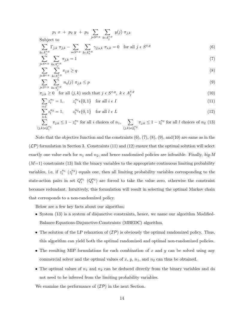
We now present the Mixed Integer Programming formulation (IP) that gives the optimal non-

randomized policy.

(IP) MIN d

λ1

∑

sεSx,y1

∑

kεAx,ys

πs,k + λ2

∑

sεSx,y2

∑

kεAx,ys

πs,k

+ w∑

jεSx,y

∑

kεAx,y

j

nq(j) πj,k +

13

p1 x + p2 y + p3

∑

jεSx,y

∑

kεAx,y

j

y(j) πj,k

Subject to∑

kεAx,y

j

Γj,k πj,k −∑

sεSx,y

∑

kεAx,ys

γj|s,k πs,k = 0 for all j ε Sx,y (6)

∑

jεSx,y

∑

kεAx,y

j

πj,k = 1 (7)

∑

jεBx,y

∑

kεAx,y

j

πj,k ≥ q (8)

∑

jεSx,y

∑

kεAx,y

j

nq(j) πj,k ≤ p (9)

πj,k ≥ 0 for all (j, k) such that j ε Sx,y, k ε Ax,yj (10)

∑

iεI

zn1

i = 1, zn1

i ε{0, 1} for all i ε I (11)

∑

lεL

zn2

l = 1, zn2

l ε{0, 1} for all l ε L (12)

∑

(j,k)εQn1

i

πj,k ≤ 1 − zn1

i for all i choices of n1,∑

(j,k)εQn2

l

πj,k ≤ 1 − zn2

l for all l choices of n2 (13)

Note that the objective function and the constraints (6), (7), (8), (9), and(10) are same as in the

(LP) formulation in Section 3. Constraints (11) and (12) ensure that the optimal solution will select

exactly one value each for n1 and n2, and hence randomized policies are infeasible. Finally, big-M

(M=1) constraints (13) link the binary variables to the appropriate continuous limiting probability

variables, i.e. if zn1

i (zn2

l ) equals one, then all limiting probability variables corresponding to the

state-action pairs in set Qn1

i (Qn2

l ) are forced to take the value zero, otherwise the constraint

becomes redundant. Intuitively, this formulation will result in selecting the optimal Markov chain

that corresponds to a non-randomized policy.

Below are a few key facts about our algorithm:

• System (13) is a system of disjunctive constraints, hence, we name our algorithm Modified-

Balance-Equations-Disjunctive-Constraints (MBEDC) algorithm.

• The solution of the LP relaxation of (IP) is obviously the optimal randomized policy. Thus,

this algorithm can yield both the optimal randomized and optimal non-randomized policies.

• The resulting MIP formulations for each combination of x and y can be solved using any

commercial solver and the optimal values of x, y, n1, and n2 can thus be obtained.

• The optimal values of n1 and n2 can be deduced directly from the binary variables and do

not need to be inferred from the limiting probability variables.

We examine the performance of (IP) in the next Section.

14

5 Computational Results

In this section, we provide computational results for (i) the economic analysis of the CDOS problem

and (ii) the computational speed of the MBEDC algorithm. It is important to note that much of

the economic analysis in this Section relies on the optimal non-randomized solution, which can be

efficiently obtained using the MBEDC algorithm. Refer to Table 1 in Section 5.4 for details on the

different choices of the parameters for the experiments in this Section. Throughout we focus on the

delay service level constraint. Similar experiments can be carried out to obtain insights specific to

the service level constraint on the average number of customers in queue.

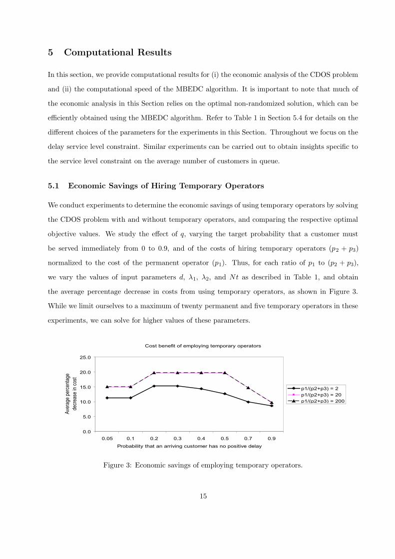
5.1 Economic Savings of Hiring Temporary Operators

We conduct experiments to determine the economic savings of using temporary operators by solving

the CDOS problem with and without temporary operators, and comparing the respective optimal

objective values. We study the effect of q, varying the target probability that a customer must

be served immediately from 0 to 0.9, and of the costs of hiring temporary operators (p2 + p3)

normalized to the cost of the permanent operator (p1). Thus, for each ratio of p1 to (p2 + p3),

we vary the values of input parameters d, λ1, λ2, and Nt as described in Table 1, and obtain

the average percentage decrease in costs from using temporary operators, as shown in Figure 3.

While we limit ourselves to a maximum of twenty permanent and five temporary operators in these

experiments, we can solve for higher values of these parameters.

Cost benefit of employing temporary operators

0.0

5.0

10.0

15.0

20.0

25.0

0.05 0.1 0.2 0.3 0.4 0.5 0.7 0.9

Probability that an arriving customer has no positive delay

Ave

rage

per

cent

age

decr

ease

in c

ost

p1/(p2+p3) = 2

p1/(p2+p3) = 20

p1/(p2+p3) = 200

Figure 3: Economic savings of employing temporary operators.

15

Over all instances in our experiments, the decrease in costs from hiring temporary operators

ranged from 0% to 26.9%. Keeping the ratio of p1 to (p2 + p3) fixed, as q is increased from 0,

initially the percentage decrease in cost increases. This is because for the case without temporary

operators the number of permanent operators required to satisfy the delay constraint increases

more than the number of operators when temporary operators are available. However, as q is

increased beyond a certain threshold value (0.3 for p1

p2+p3=2), there is no increase in the number of

operators for the case without temporary operators, as enough have been hired to over-satisfy the

constraint. In contrast, the number of operators continues to increase in the case with temporary

operators, because the use of temporary operators provides “finer control” on dealing with the delay

constraint. Thus, the percentage decrease in cost begins to fall after this point. Thus, it seems that

the value of temporary operators in the case of very stringent or very relaxed service constraints is

lower compared to the case where service constraints have moderate targets. It is in this moderate

case that the flexibility offered by temporary operators is most valuable, because if constraints are

very strict many permanent and few temporary operators are needed; or if constraints are very lax

few operators are needed in general.

We also find that, as the cost of using temporary operators compared to the cost of using

permanent operators becomes cheaper (the ratio of p1 to p2 + p3 increases) for a fixed value of q,

the percentage decrease in costs increases. But, as the above ratio is increased beyond a certain

critical level, there is no further increase in the percentage decrease in costs. This is because we

limit the maximum number of temporary operators that can be used; once the optimal number

of temporary operators to be used reaches this maximum limit the costs no longer decrease. This

indicates a need for increasing the maximum number of temporary operators available to the system.

We now move to studying some specific experimental instances to gain further, more detailed

insights.

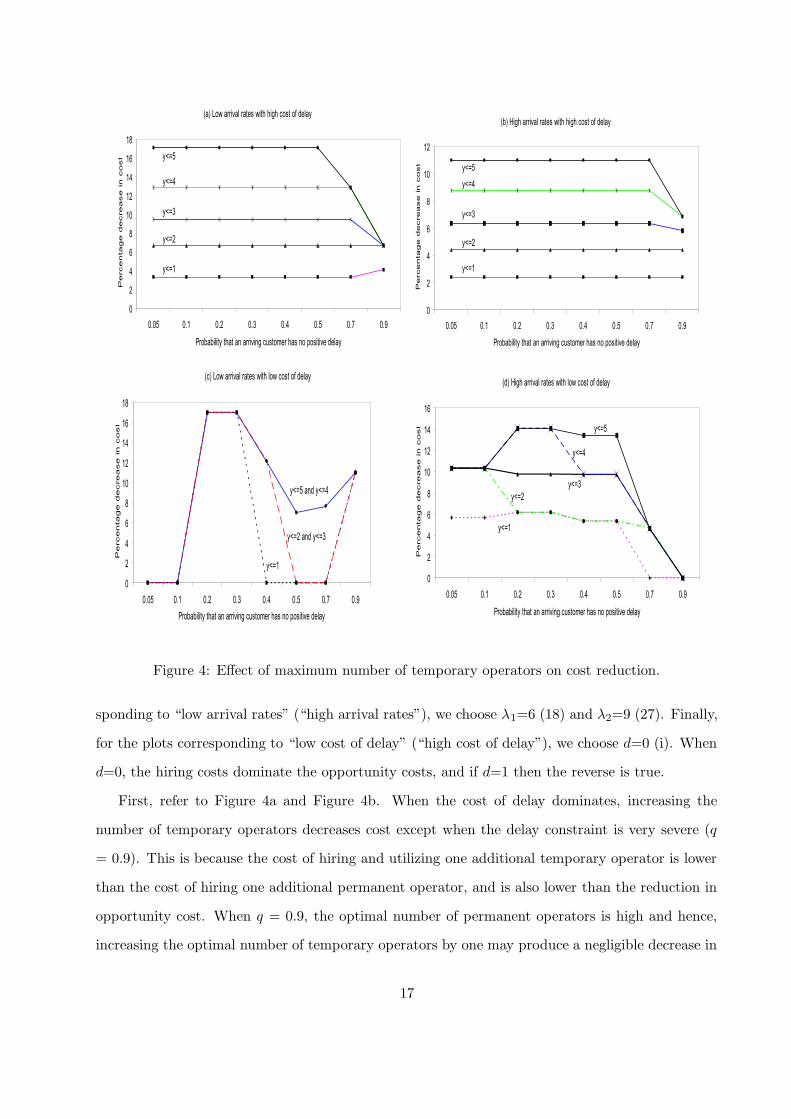
5.2 Effect of Maximum Number of Temporary Operators Available

Given the affect of our limit on the number of temporary operators in Section 5.1, we now study

the effect of the maximum number of temporary operators available on the reduction in cost for

different values of q. These results are presented in Figure 4.

We fix w=0, p1=1, p2=0.1, p3=0.4, Nt=150, α(i) = β(i)=5, µ1 = µ2=2. For the plots corre-

16

(a) Low arrival rates with high cost of delay

0

2

4

6

8

10

12

14

16

18

0.05 0.1 0.2 0.3 0.4 0.5 0.7 0.9

Probability that an arriving customer has no positive delay

Percentage decrease in

cost

y<=1

y<=5

y<=4

y<=3

y<=2

(b) High arrival rates with high cost of delay

0

2

4

6

8

10

12

0.05 0.1 0.2 0.3 0.4 0.5 0.7 0.9

Probability that an arriving customer has no positive delay

Percentage decrease in

cost

y<=1

y<=5

y<=4

y<=3

y<=2

(c) Low arrival rates with low cost of delay

0

2

4

6

8

10

12

14

16

18

0.05 0.1 0.2 0.3 0.4 0.5 0.7 0.9

Probability that an arriving customer has no positive delay

Percentage decrease in

cost

y<=5 and y<=4

y<=1

y<=2 and y<=3

(d) High arrival rates with low cost of delay

0

2

4

6

8

10

12

14

16

0.05 0.1 0.2 0.3 0.4 0.5 0.7 0.9

Probability that an arriving customer has no positive delay

Percentage decrease in

cost

y<=1

y<=5

y<=4

y<=3

y<=2

Figure 4: Effect of maximum number of temporary operators on cost reduction.

sponding to “low arrival rates” (“high arrival rates”), we choose λ1=6 (18) and λ2=9 (27). Finally,

for the plots corresponding to “low cost of delay” (“high cost of delay”), we choose d=0 (i). When

d=0, the hiring costs dominate the opportunity costs, and if d=1 then the reverse is true.

First, refer to Figure 4a and Figure 4b. When the cost of delay dominates, increasing the

number of temporary operators decreases cost except when the delay constraint is very severe (q

= 0.9). This is because the cost of hiring and utilizing one additional temporary operator is lower

than the cost of hiring one additional permanent operator, and is also lower than the reduction in

opportunity cost. When q = 0.9, the optimal number of permanent operators is high and hence,

increasing the optimal number of temporary operators by one may produce a negligible decrease in

17

the opportunity cost of delay. We also note that as the arrival rates (both λ1 and λ2) are increased,

the value of the temporary operators decreases; or in other words, to obtain the same percentage

decrease in cost, more temporary operators are required as the arrival rate increases. This is logical,

as each operator’s relative effect on the system is diminished.

Refer now to Figure 4c and Figure 4d. Since d=0, the hiring costs dominate and the delay

constraint restricts feasibility. In such a situation, we observe that for different intervals of the

value of q, we get very different optimal numbers of temporary operators, and that the number

may increase and decrease without a clear pattern. (It increases from 1 to 2 to 4 in Figure 4c and

it increases from 2 to 4 to 5 and then decreases from 5 to 2 to 1 in Figure 4d.) The explanation

is as follows. Without any temporary operators, the number of permanent operators required to

satisfy the delay constraint increases with q. If temporary operators are allowed, it will be optimal

to hire some (r) number of temporary operators for a particular value of q only if they replace

and are cheaper than a permanent operator. This substitution is permitted only if the resulting

queueing system still satisfies the delay constraint for that value of q. Thus, we only add temporary

operators in “bundles” of size r, where r may change with q.

From these experiments we see that if the relative magnitude of d dominates hiring costs then

each additional temporary operator is effective at reducing costs up until the constraint is very

strict. In contrast, if d is small (or only enforced via constraint), temporary operators must be

hired in “bundles” to replace a permanent operator. Thus, assessing the magnitude of d is crucial.

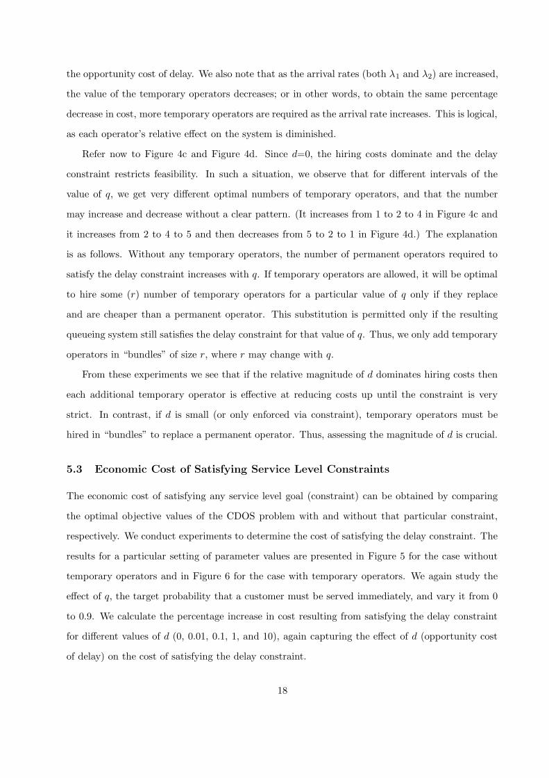
5.3 Economic Cost of Satisfying Service Level Constraints

The economic cost of satisfying any service level goal (constraint) can be obtained by comparing

the optimal objective values of the CDOS problem with and without that particular constraint,

respectively. We conduct experiments to determine the cost of satisfying the delay constraint. The

results for a particular setting of parameter values are presented in Figure 5 for the case without

temporary operators and in Figure 6 for the case with temporary operators. We again study the

effect of q, the target probability that a customer must be served immediately, and vary it from 0

to 0.9. We calculate the percentage increase in cost resulting from satisfying the delay constraint

for different values of d (0, 0.01, 0.1, 1, and 10), again capturing the effect of d (opportunity cost

of delay) on the cost of satisfying the delay constraint.

18

Economic cost of satisfying the delay constraint

with only permanent operators

0

20

40

60

80

100

120

0.05 0.1 0.2 0.3 0.4 0.5 0.7 0.9

Probability that an arriving customer has no positive delay

Per

cent

age

incr

ease

in c

ost d = 0

d = 0.01

d = 0.1

d = 1 d = 10A

B C

Figure 5: Economic cost of satisfying the delay constraint with permanent operators only.

λ1 = 18, λ2 = 27, µ1 = µ2 = 2, α(i) = 0.5, β(i) = 0.5, Nt = 150, w = 0, p1 = 1, p2 = 0.1, p3 = 0.4.

Figure 5 shows that for a given value of d, the delay constraint is redundant up to a certain

value of q, q(d) which is increasing in d, and hence there is no increase in costs up to this value

q(d) (q=0.1 for d ≤0.01; q=0.5 for d=0.1). As expected the percentage cost of satisfying the delay

constraint is increasing in q, keeping all other parameters fixed. One feature of note from Figure 5

are the “plateaus” in the increase in cost. Refer to the points marked A, B and C, which correspond

to using four, five and five permanent operators, respectively when d=0. An increase in q from 0.1

to 0.2 caused the optimal solution to increase the number of permanent operators by one. Ideally,

if we have five permanent operators, we would prefer to be at point C, where we are satisfying the

highest service level goal for delay possible with five permanent operators. At point B, keeping five

permanent operators on staff over-satisfies the constraint, and wastes money.

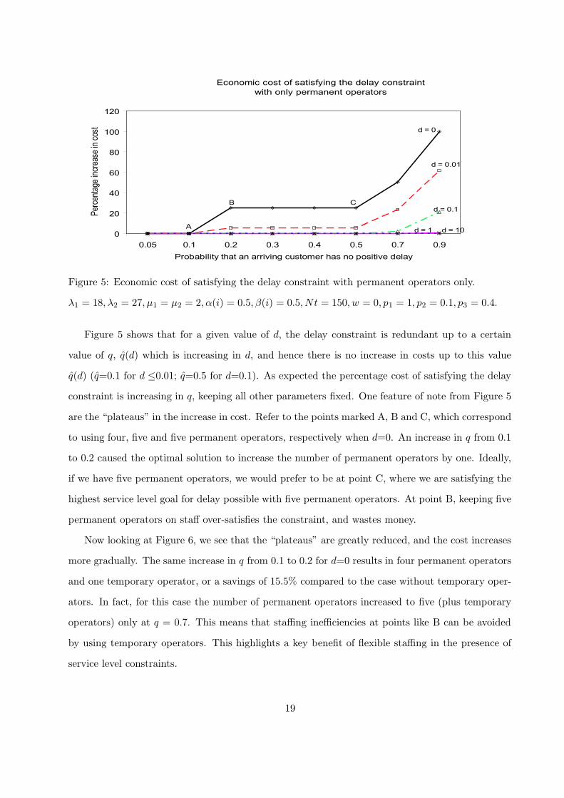
Now looking at Figure 6, we see that the “plateaus” are greatly reduced, and the cost increases

more gradually. The same increase in q from 0.1 to 0.2 for d=0 results in four permanent operators

and one temporary operator, or a savings of 15.5% compared to the case without temporary oper-

ators. In fact, for this case the number of permanent operators increased to five (plus temporary

operators) only at q = 0.7. This means that staffing inefficiencies at points like B can be avoided

by using temporary operators. This highlights a key benefit of flexible staffing in the presence of

service level constraints.

19

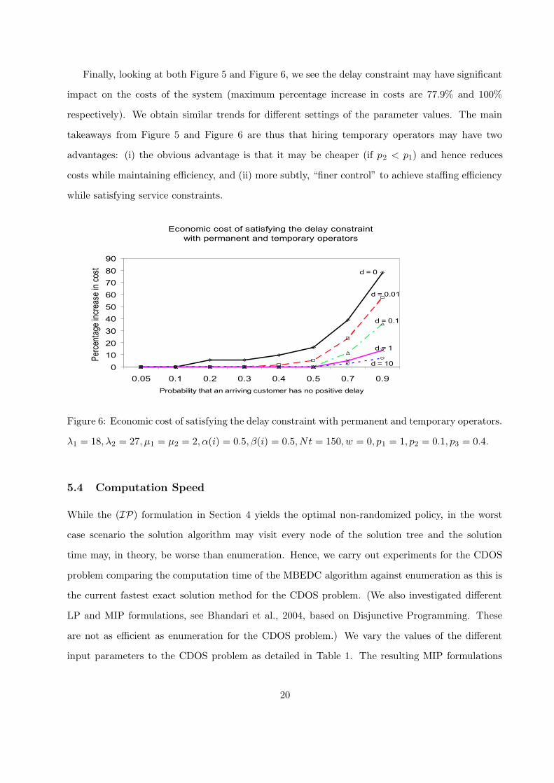
Finally, looking at both Figure 5 and Figure 6, we see the delay constraint may have significant

impact on the costs of the system (maximum percentage increase in costs are 77.9% and 100%

respectively). We obtain similar trends for different settings of the parameter values. The main

takeaways from Figure 5 and Figure 6 are thus that hiring temporary operators may have two

advantages: (i) the obvious advantage is that it may be cheaper (if p2 < p1) and hence reduces

costs while maintaining efficiency, and (ii) more subtly, “finer control” to achieve staffing efficiency

while satisfying service constraints.

Economic cost of satisfying the delay constraint

with permanent and temporary operators

0

10

20

30

40

50

60

70

80

90

0.05 0.1 0.2 0.3 0.4 0.5 0.7 0.9

Probability that an arriving customer has no positive delay

Per

cent

age

incr

ease

in c

ost

d = 0

d = 0.1

d = 0.01

d = 1

d = 10

Figure 6: Economic cost of satisfying the delay constraint with permanent and temporary operators.

λ1 = 18, λ2 = 27, µ1 = µ2 = 2, α(i) = 0.5, β(i) = 0.5, Nt = 150, w = 0, p1 = 1, p2 = 0.1, p3 = 0.4.

5.4 Computation Speed

While the (IP) formulation in Section 4 yields the optimal non-randomized policy, in the worst

case scenario the solution algorithm may visit every node of the solution tree and the solution

time may, in theory, be worse than enumeration. Hence, we carry out experiments for the CDOS

problem comparing the computation time of the MBEDC algorithm against enumeration as this is

the current fastest exact solution method for the CDOS problem. (We also investigated different

LP and MIP formulations, see Bhandari et al., 2004, based on Disjunctive Programming. These

are not as efficient as enumeration for the CDOS problem.) We vary the values of the different

input parameters to the CDOS problem as detailed in Table 1. The resulting MIP formulations

20

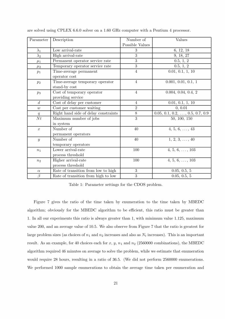
are solved using CPLEX 6.6.0 solver on a 1.60 GHz computer with a Pentium 4 processor.

Parameter Description Number of ValuesPossible Values

λ1 Low arrival-rate 3 6, 12, 18

λ2 High arrival-rate 3 9, 18, 27

µ1 Permanent operator service rate 3 0.5, 1, 2

µ2 Temporary operator service rate 3 0.5, 1, 2

p1 Time-average permanent 4 0.01, 0.1, 1, 10operator cost

p2 Time-average temporary operator 4 0.001, 0.01, 0.1, 1stand-by cost

p3 Cost of temporary operator 4 0.004, 0.04, 0.4, 2providing service

d Cost of delay per customer 4 0.01, 0.1, 1, 10

w Cost per customer waiting 2 0, 0.01

q Right hand side of delay constraints 8 0.05, 0.1, 0.2, . . . , 0.5, 0.7, 0.9

Nt Maximum number of jobs 3 50, 100, 150in system

x Number of 40 4, 5, 6, . . . , 43permanent operators

y Number of 40 1, 2, 3, . . . , 40temporary operators

n1 Lower arrival-rate 100 4, 5, 6, . . . , 103process threshold

n2 Higher arrival-rate 100 4, 5, 6, . . . , 103process threshold

α Rate of transition from low to high 3 0.05, 0.5, 5

β Rate of transition from high to low 3 0.05, 0.5, 5

Table 1: Parameter settings for the CDOS problem.

Figure 7 gives the ratio of the time taken by enumeration to the time taken by MBEDC

algorithm; obviously for the MBEDC algorithm to be efficient, this ratio must be greater than

1. In all our experiments this ratio is always greater than 1, with minimum value 1.125, maximum

value 200, and an average value of 10.5. We also observe from Figure 7 that the ratio is greatest for

large problem sizes (as choices of n1 and n2 increases and also as Nt increases). This is an important

result. As an example, for 40 choices each for x, y, n1 and n2 (2560000 combinations), the MBEDC

algorithm required 46 minutes on average to solve the problem, while we estimate that enumeration

would require 28 hours, resulting in a ratio of 36.5. (We did not perform 2560000 enumerations.

We performed 1000 sample enumerations to obtain the average time taken per enumeration and

21

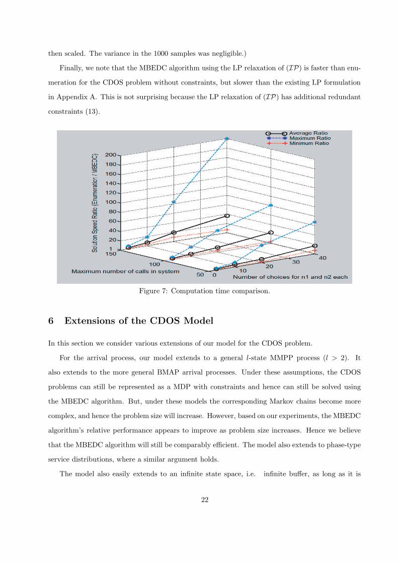
then scaled. The variance in the 1000 samples was negligible.)

Finally, we note that the MBEDC algorithm using the LP relaxation of (IP) is faster than enu-

meration for the CDOS problem without constraints, but slower than the existing LP formulation

in Appendix A. This is not surprising because the LP relaxation of (IP) has additional redundant

constraints (13).

Figure 7: Computation time comparison.

6 Extensions of the CDOS Model

In this section we consider various extensions of our model for the CDOS problem.

For the arrival process, our model extends to a general l-state MMPP process (l > 2). It

also extends to the more general BMAP arrival processes. Under these assumptions, the CDOS

problems can still be represented as a MDP with constraints and hence can still be solved using

the MBEDC algorithm. But, under these models the corresponding Markov chains become more

complex, and hence the problem size will increase. However, based on our experiments, the MBEDC

algorithm’s relative performance appears to improve as problem size increases. Hence we believe

that the MBEDC algorithm will still be comparably efficient. The model also extends to phase-type

service distributions, where a similar argument holds.

The model also easily extends to an infinite state space, i.e. infinite buffer, as long as it is

22

infinite in only one dimension. This is because the resulting Markov chain repeats after some finite

state, so it can be analyzed using the matrix analytic technique (Neuts, 1981). Intuitively, the

infinite state space Markov chain can be transformed into a equivalent finite state space Markov

chain. The computational results for the infinite state space (infinite buffer) problem are identical

to the results in Figure 7.

7 Conclusions

The CDOS problem is a very relevant problem not only in call centers but in many other service

industries such as flexible Internet servers (Akamai Technologies, www.akamai.com), restaurants,

grocery stores, etc. The key factor all of these businesses have in common is that service level goals

are important, and hence must be included in their operational model. Traditionally, these goals

have been included as opportunity costs, but such costs are difficult to estimate, whereas modeling

the goals as constraints is straightforward.

We find these opportunity costs have a tremendous effect on the optimal number of temporary

operators (cf. Section 5.2) and hence it is crucial they are accurately estimated. In our experiments

we also find that in most cases it was optimal to use at least one temporary operator, even if there

are no service level constraints. Moreover, the value of flexibility provided by temporary operators

in the case of very stringent or very relaxed service constraints tended to be lower compared to the

case where service constraints have moderate targets.

Assuming one can estimate the opportunity costs accurately, their magnitude relative to the

hiring costs determines the effectiveness of temporary operators. If opportunity costs dominate,

then each additional temporary operator is effective at reducing costs up until a service level

constraint is very strict. In contrast, if the opportunity costs are small (or only enforced via

constraint), temporary operators must be hired in “bundles”, to replace a permanent operator.

Finally, satisfying a service level constraint (beyond some minimal threshold level) imposes costs

on a service provider. Temporary operators can be an important tool in reducing these costs, as

they provide finer staffing control for the call center manager. While we focused on a probability

of no-delay constraint, the economic cost of satisfying any service level goal (constraint) can be

obtained similarly, by comparing the optimal objective values of the CDOS problem with and

without that particular constraint, respectively.

23

The MBEDC algorithm is an efficient, exact solution method for the CDOS problem and its

relative performance improves over enumeration as the problem size increases. While we imple-

mented the MBEDC algorithm for a continuous-time problem in this paper, the algorithm is in fact

more general and can be applied to a discrete-time stochastic constrained optimization problem

as well. We plan to implement the MBEDC algorithm for an inventory management case study

with fill rate constraints. In general, the MBEDC algorithm can be used in two ways: (i) Direct

implementation to find optimal solutions in real time for real world problems or (ii) To benchmark

heuristics (instead of lower/upper bounds) for real world problems.

In the future we also plan to study: (i) CDOS problem with multiple customer classes, and

(ii) CDOS problem where the manager only needs to satisfy l of the L service level goals using

Disjunctive Programming techniques (Balas, 1998). In the infinite buffer CDOS problem with

multiple customer classes, applying the matrix analytic method is more difficult as the resulting

Markov chains will be infinite in multiple dimensions. However, an approximation scheme called

dimensionality reduction has been proposed for such problems in Harchol-Balter et al. (2003).

References

Akamai Technologies, Inc. 2003. Akamai Technologies: Technical overview. Akamai Technologies

White Paper, www.akamai.com.

Andrews, B. H. and H. L. Parsons. 1993. Establishing telephone agent staffing levels through

economic optimization. Interfaces 23 14-20.

Balas, E. 1998. Disjunctive Programming: Properties of the convex hull of feasible points. Discrete

Applied Mathematics 89(1-3) 3-44.

Bertsekas, D. 1995. Dynamic Programming and Optimal Control, Volume Two, Athena Scientific,

Belmont Massachusetts.

Bhandari, A., A. Scheller-Wolf and M. Harchol-Balter. 2004. Exact solution methods for general

parameter-dependent-Markov-chain-optimization problems. Working Paper, Tepper School of

Business, Carnegie Mellon University.

Brigandi, A. J., D.R. Dargon, M.J. Sheehan and T. Spencer III. 1994. AT&T’s call processing

simulator (CAPS) operational design for inbound call centers. Interfaces 24 6-28.

24

Deniz, B., I. Karaesmen and A. Scheller-Wolf. 2005. Managing inventories of perishable goods.

Working Paper, Tepper School of Business, Carnegie Mellon University.

Gans, N., G. Koole and A. Mandelbaum. 2003. Telephone call centers: Tutorial, review and re-

search prospects. Invited review paper by Manufacturing and Service Operations Management

(M&SOM), 5 79-141.

Hall R. 1991. Queueing Methods for Services and Manufacturing, Prentice Hall, Englewood Cliffs,

New Jersey.

Harchol-Balter, M., C. Li, T. Osogami, A. Scheller-Wof and M. Squillante. 2003. Task assignment

with cycle stealing under central queue. 23rd International Conference on Distributed Computing

Systems (ICDCS ’03) , Providence, RI.

Ingolfsson, A., M. A. Haque and A. Umnikov. 2002. Accounting for time-varying queueing effects

in workforce scheduling. Eur. J. Oper. Res. 139 585-597.

Jennings, O., A. Mandelbaum, W. Massey and W. Whitt. 1996. Server staffing to meet time-varying

demand. Management Science 42 1383-1394.

Jongbloed, G. and G. M. Koole. 2001. Managing uncertainty in call centers using Poisson mixtures.

Appl. Stochastic Models in Bus. Indust. 17 307-318.

Lucantoni, D. 1993. The BMAP/G/1 queue: A tutorial. Performance/SIGMETRICS Tutorials.

330-358.

Nain, P. and R. Nunez-Queija. 2001. An M/M/1 queue in a semi-Markovian environment. Pro-

ceedings of the ACM SIGMETRICS / Performance 2001 Conference, Cambridge, Massachusetts,

268-278.

Nemhauser, G. and L. Wolsey. 1988. Integer and Combinatorial Optimization, John Wiley & Sons,

New York, New York.

Neuts, M. 1981. Matrix-Geometric Solutions in Stochastic Models. Johns Hopkins University Press,

Baltimore, Maryland.

Osogami, T. and M. Harchol-Balter. 2003. Necessary and sufficient conditions for representing

general distributions by Coxians. 13th International Conference on Modeling Techniques and

Tools for Computer Performance Evaluation, Urbana, Illinois 182-199.

25

Porteus, E. 2002. Foundations of Stochastic Inventory Theory, Stanford University Press, Stanford

California.

Puterman, M. 1994. Markov Decision Processes: Discrete Stochastic Dynamic Programming, John

Wiley and Sons, New York, New York.

Veeraraghavan, S. and A. Scheller-Wolf. 2005. Now or Later: A simple policy for effective dual

sourcing in a capacitated environment. Working Paper, Tepper School of Business, Carnegie

Mellon University.

Whitt, W. 1999. Dynamic staffing in a telephone call center aiming to immediately answer all calls.

Operations Resarch Letters, 24 205-212.

Wong, H., G. J. Van Houtum, D. Cattrysse and D. Van Oudheusden. 2006. Multi-item spare

parts systems with lateral transshipments and waiting time constraints. European Journal of

Operational Research, to appear.

Yoo, J. 1996. Queueing models for staffing service operations, Ph.D. dissertation, University of

Maryland, College Park, MD.

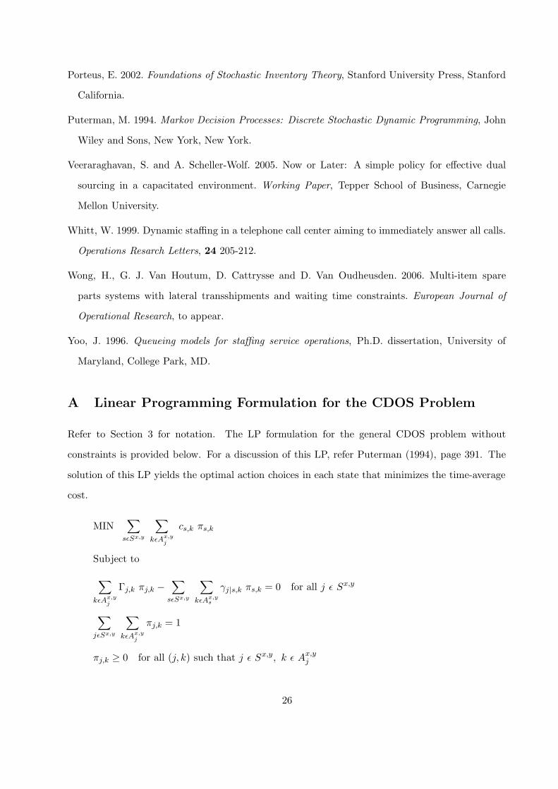
A Linear Programming Formulation for the CDOS Problem

Refer to Section 3 for notation. The LP formulation for the general CDOS problem without

constraints is provided below. For a discussion of this LP, refer Puterman (1994), page 391. The

solution of this LP yields the optimal action choices in each state that minimizes the time-average

cost.

MIN∑

sεSx,y

∑

kεAx,y

j

cs,k πs,k

Subject to

∑

kεAx,y

j

Γj,k πj,k −∑

sεSx,y

∑

kεAx,ys

γj|s,k πs,k = 0 for all j ε Sx,y

∑

jεSx,y

∑

kεAx,y

j

πj,k = 1

πj,k ≥ 0 for all (j, k) such that j ε Sx,y, k ε Ax,yj

26

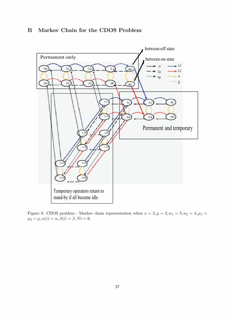
B Markov Chain for the CDOS Problem

µ

2µ

4µ

λ1

λ2

α

β

a

bb

Permanent only

Permanent and temporary

Temporary operators return to

stand-by if all become idle

between-off state

between-on state

Figure 8: CDOS problem - Markov chain representation when x = 2, y = 2, n1 = 5, n2 = 4, µ1 =µ2 = µ, α(i) = α, β(i) = β,Nt = 6.

27