An EVT primer for credit risk

Valerie Chavez-Demoulin

EPF Lausanne, Switzerland

Paul Embrechts

ETH Zurich, Switzerland

First version: December 2008

This version: May 25, 2009

Abstract

We review, from the point of view of credit risk management, classical Extreme

Value Theory in its one–dimensional (EVT) as well as more–dimensional (MEVT)

setup. The presentation is highly coloured by the current economic crisis against which

background we discuss the (non–)usefulness of certain methodological developments.

We further present an outlook on current and future research for the modelling of

extremes and rare event probabilities.

Keywords: Basel II, Copula, Credit Risk, Dependence Modelling, Diversification, Extreme

Value Theory, Regular Variation, Risk Aggregation, Risk Concentration, Subprime Crisis.

1 Introduction

It is September 30, 2008, 9.00 a.m. CET. Our pen touches paper for writing a first version

of this introduction, just at the moment that European markets are to open after the US

Congress in a first round defeated the bill for a USD 700 Bio fund in aid of the financial

1

industry. The industrialised world is going through the worst economic crisis since the

Great Depression of the 1930s. It is definitely not our aim to give an historic overview of

the events leading up to this calamity, others are much more competent for doing so; see

for instance Crouhy et al. [13] and Acharya and Richardson [1]. Nor will we update the

events, now possible in real time, of how this crisis evolves. When this article is in print, the

world of finance will have moved on. Wall Street as well as Main Street will have taken the

consequences. The whole story started with a credit crisis linked to the American housing

market. The so–called subprime crisis was no doubt the trigger, the real cause however

lies much deeper in the system and does worry the public much, much more. Only these

couple of lines should justify our contribution as indeed two words implicitly jump out of

every public communication on the subject: extreme and credit. The former may appear in

the popular press under the guise of a Black Swan (Taleb [25]) or a 1 in 1000 year event,

or even as the unthinkable. The latter presents itself as a liquidity squeeze, or a drying up

of interbank lending, or indeed the subprime crisis. Looming above the whole crisis is the

fear for a systemic risk (which should not be confused with systematic risk) of the world’s

financial system; the failure of one institution implies, like a domino effect, the downfall

of others around the globe. In many ways the worldwide regulatory framework in use,

referred to as the Basel Capital Accord, was not able to stem such a systemic risk, though

early warnings were available; see Danıelsson et al. [14]. So what went wrong? And more

importantly, how can we start fixing the system. Some of the above references give a first

summary of proposals.

It should by now be abundantly clear to anyone only vaguely familiar with some of the

technicalities underlying modern financial markets, that answering these questions is a very

tough call indeed. Any solution that aims at bringing stability and healthy, sustainable

growth back into the world economy can only be achieved by very many efforts from all

sides of society. Our paper will review only one very small methodological piece of this

global jigsaw–puzzle, Extreme Value Theory (EVT). None of the tools, techniques, regulatory

guidelines or political decisions currently put forward will be the panacea ready to cure all

the diseases of the financial system. As scientists, we do however have to be much more

2

forthcoming in stating why certain tools are more useful than others, and also why some are

definitely ready for the wastepaper basket. Let us mention one story here to make a point.

One of us, in September 2007, gave a talk at a conference attended by several practitioners

on the topic of the weaknesses of VaR–based risk management. In the ensuing round table

discussion, a regulator voiced humbleness saying that, after that critical talk against VaR,

one should perhaps rethink some aspects of the regulatory framework. To which the Chief

Risk Officer of a bigger financial institution sitting next to him whispered “No, no, you are

doing just fine.” It is this “stick your head in the sand” kind of behaviour we as scientists

have the mandate to fight against.

So this paper aims at providing the basics any risk manager should know on the modelling

of extremal events, and this from a past–present–future research perspective. Such events

are often also referred to as low probability events or rare events, a language we will use

interchangeably throughout this paper. The choice of topics and material discussed are

rooted in finance, and especially in credit risk. In Section 2 we start with an overview of

the credit risk specific issues within Quantitative Risk Management (QRM) and show where

relevant EVT related questions are being asked. Section 3 presents the one–dimensional

theory of extremes, whereas Section 4 is concerned with the multivariate case. In Section 5

we discuss particular applications and give an outlook on current research in the field. We

conclude in Section 6.

Though this paper has a review character, we stay close to an advice once given to us by

Benoit Mandelbrot: “Never allow more than ten references to a paper.” We will not be able

to fully adhere to this principle, but we will try. As a consequence, we guide the reader to

some basic references which best suit the purpose of the paper, and more importantly, that

of its authors. Some references we allow ourselves to be mentioned from the start. Whenever

we refer to QRM, the reader is expected to have McNeil et al. [20] (referred to throughout as

MFE) close at hand for further results, extra references, notation and background material.

Similarly, an overview of one–dimensional EVT relevant for us is Embrechts et al. [17] (EKM).

For general background on credit risk, we suggest Bluhm and Overbeck [8] and the relevant

chapters in Crouhy et al. [12]. The latter text also provides a more applied overview of

3

financial risk management.

2 Extremal events and credit risk

Credit risk is presumably the oldest risk type facing a bank: it is the risk that the originator

of a financial product (a mortgage, say) faces as a function of the (in)capability of the obligor

to honour an agreed stream of payments over a given period of time. The reason we recall

the above definition is that, over the recent years, credit risk has become rather difficult to

put ones finger on. In a meeting several years ago, a banker asked us “Where is all the credit

risk hiding?” ... If only one had taken this question more seriously at the time. Modern

product development, and the way credit derivatives and structured products are traded on

OTC markets, have driven credit risk partly into the underground of financial markets. One

way of describing “underground” for banks no doubt is “off–balance sheet”. Also regulators

are becoming increasingly aware of the need for a combined view on market and credit

risk. A most recent manifestation of this fact is the new regulatory guideline (within the

Basel II framework) for an incremental risk charge (IRC) for all positions in the trading

book with migration/default risk. Also, regulatory arbitrage drove the creativity of (mainly)

investment banks to singular heights trying to repackage credit risk in such a way that the

bank could get away with a minimal amount of risk capital. Finally, excessive leverage

allowed to increase the balance sheet beyond any acceptable level, leading to extreme losses

when markets turned and liquidity dried up.

For the purpose of this paper, below we give examples of (in some cases, comments on)

credit risk related questions where EVT technology plays (can/should play) a role. At this

point we like to stress that, though we very much resent the silo thinking still found in risk

management, we will mainly restrict to credit risk related issues. Most of the techniques

presented do however have a much wider range of applicability; indeed, several of the results

basically come to life at the level of risk aggregation and the holistic view on risk.

Example 1. Estimation of default probabilities (DP). Typically, the DP of a credit (insti-

4

tution) over a given time period [0, T ], say, is the probability that at time T , the value of the

institution, V (T ), falls below the (properly defined) value of debt D(T ), hence for institu-

tion i, PDi(T ) = P (Vi(T ) < Di(T )). For good credits, these probabilities are typically very

small, hence the events {Vi(T ) < Di(T )} are rare or extreme. In credit rating agency language

(in this example, Moody’s), for instance for T = 1 year, PDA(1) = 0.4%, PDB(1) = 4.9%,

PDAa(1) = 0.0%, PDBa(1) = 1.1%. No doubt recent events will have changed these num-

bers, but the message is clear: for good quality credits, default was deemed very small.

This leads to possible applications of one–dimensional EVT. A next step would involve the

estimation of the so–called LGD, loss given default. This is typically an expected value of

a financial instrument (a corporate bond, say) given that the rare event of default has taken

place. This naturally leads to threshold or exceedance models; see Section 4, around (29).

Example 2. In portfolio models, several credit risky securities are combined. In these

cases one is not only interested in estimating the marginal default probabilities PDi(T ),

i = 1, . . . , d, but much more importantly the joint default probabilities, for I ⊂ d = {1, . . . , d}

PDId(T ) = P ({Vi(T ) < Di(T ), i ∈ I} ∩ {Vj(T ) ≥ Dj(T ), j ∈ d\I}) . (1)

For this kind of problems multivariate EVT (MEVT) presents itself as a possible tool.

Example 3. Based on models for (1), structured products like ABSs, CDOs, CDSs, MBSs,

CLOs, credit baskets etc. can (hopefully) be priced and (even more hopefully) hedged. In

all of these examples, the interdependence (or more specifically, the copula) between the

underlying random events plays a crucial role. Hence we need a better understanding of

the dependence between extreme (default) events. Copula methodology in general has been

(mis)used extensively in this area. A critical view on the use of correlation is paramount

here.

Example 4. Instruments and portfolios briefly sketched above are then aggregated at the

global bank level, their risk is measured and the resulting numbers enter eventually into the

Basel II capital adequacy ratio of the bank. If we abstract from the precise application, one

is typically confronted with r risk measures RM1, . . . , RMr, each of which aims at estimating

a rare event like RMi = VaRi,99.9(T = 1), the 1–year, 99.9% Value–at–Risk for position i.

5

Besides the statistical estimation (and proper understanding!) of such risk measures, the

question arises how to combine r risk measures into one number (given that this would make

sense) and how to take possible diversification and concentration effects into account. For

a better understanding of the underlying problems, (M)EVT enters here in a fundamental

way. Related problems involve scaling, both in the confidence level as well as the time

horizon underlying the specific risk measure. Finally, backtesting the statistical adequacy of

the risk measure used is of key importance. Overall, academic worries on how wise it is to

keep on using VaR–like risk measures ought to be taken more seriously.

Example 5. Simulation methodology. Very few structured products in credit can be priced

and hedged analytically. I.e. numerical as well as simulation/Monte Carlo tools are called for.

The latter lead to the important field of rare event simulation and resampling of extremal

events. Under resampling schemes we think for instance of the bootstrap, the Jackknife

and cross validation. Though these techniques do not typically belong to standard (M)EVT,

knowing about their strengths and limitations, especially for credit risk analysis, is extremely

important. A more in depth knowledge of EVT helps in better understanding the properties

of such simulation tools. We return to this topic later in Section 5.

Example 6. In recent crises, as there are LTCM and the subprime crisis, larger losses often

occurred because of the sudden widening of credit spreads, or the simultaneous increase in

correlations between different assets; a typical diversification breakdown. Hence one needs

to investigate the influence of extremal events on credit spreads and measures of dependence,

like correlation. This calls for a time dynamic theory, i.e. (multivariate) extreme value theory

for stochastic processes.

Example 7 (Taking Risk to Extremes). This is the title of an article by Mara der

Hovanesian in Business Week of May 23, 2005(!). It was written in the wake of big hedge

fund losses due to betting against GM stock while piling up on GM debt. The subtitle of

the article reads “Will derivatives cause a major blowup in the world’s credit markets?” By

now we (unfortunately) know that they did! Several quotes from the above article early on

warned about possible (very) extreme events just around the corner:

6

– “... a possible meltdown in credit derivatives if investors all tried to run for the exit at

the same time.” (IMF).

– “... the rapid proliferation of derivatives products inevitably means that some will not

have been adequately tested by market stress.” (Alan Greenspan).

– “It doesn’t need a 20% default rate across the corporate universe to set off a selling

spree. One or two defaults can be very destructive.” (Anton Pil).

– “Any apparently minor problem, such as a flurry of downgrades, could quickly engulf

the financial system by sending markets into a tailspin, wiping out hedge funds, and

dragging down banks that lent them money.”

– “Any unravelling of CDOs has the potential to be extremely messy. There’s just no

way to measure what’s at stake.” (Peter J. Petas).

The paper was about a potential credit tsunami and the way banks were using such deriva-

tives products not as risk management tools, but rather as profit machines. All of the above

disaster prophecies came true and much worse; extremes ran havoc. It will take many years

to restore the (financial) system and bring it to the level of credibility a healthy economy

needs.

Example 8 (A comment on “Who’s to blame”). Besides the widespread view about

“The secret formula that destroyed Wall Street” (see also Section 5, in particular (31)),

putting the blame for the current crisis in the lap of the financial engineers, academic

economists also have to ask themselves some soul–searching questions. Some even speak

of “A systemic failure of academic economics”. Concerning mathematical finance having to

take the blame, I side more with Roger Guesnerie (College de France) who said “For this

crisis, mathematicians are innocent . . . and this in both meanings of the word”. Having

said that, mathematicians have to take a closer look at practice and communicate much

more vigorously the conditions under which their models are derived; see also the quotes in

Example 10. The resulting Model Uncertainty for us is the key quantitative problem going

forward; more on this later in the paper. See also the April 2009 publication “Supervisory

7

guidance for assessing banks’ financial instrument fair value practices” by the Basel Com-

mittee on Banking Supervision. In it, it is stressed that “While qualitative assessments are

a useful starting point, it is desirable that banks develop methodologies that provide, to the

extent possible, quantitative assessments (for valuation uncertainty).”

Example 9 (A comment on “Early warning”). Of course, as one would expect just

by the Law of Large Numbers, there were warnings early on. We all recall Warren Buffett’s

famous reference to (credit) derivatives as “Financial weapons of mass distructions”. On

the other hand, warnings like Example 7 and similar ones were largely ignored. What

worries us as academics however much more is that seriously researched and carefully written

documents addressed at the relevant regulatory or political authorities often met with total

indifference or even silence. For the current credit crisis, a particularly worrying case is

the November 7, 2005 report by Harry Markopolos mailed to the SEC referring to Madoff

Investment Securities, LLC, as “The world’s largest hedge fund is a fraud”. Indeed, in a very

detailed analysis, the author shows that Madoff’s investment strategy is a Ponzi scheme,

and this already in 2005! Three and a half years later and for some, several billion dollars

poorer, we all learned unfortunately the hard and unpleasant way. More than anything

else, the Markopolos Report clearly proves the need for quantitative skills on Wall Street:

read it! During the Congressional hearings on Madoff, Markopolos referred to the SEC as

being “over–lawyered”. From our personal experience, we need to mention Danıelsson et al.

[14]. This critical report was written as an official response to the, by then, new Basel II

guidelines and was addressed to the Basel Committee on Banking Supervision. In it, some

very critical comments were made on the overly use of VaR–technology and how the new

guidelines “. . .taken altogether, will enhance both the procyclicality of regulation and the

susceptibility of the financial system to systemic crises, thus negating the central purpose

of the whole exercise. Reconsider before it is too late.” Unfortunately, also this report met

with total silence, and most unfortunately, it was dead right with its warnings!

Example 10 (The Turner Review). It is interesting to see that in the recent Turner

Review, “A regulatory response to the global banking crisis”, published in March 2009 by

the FSA, among many more things, the bad handling of extreme events and the problems

8

underlying VaR–based risk management were highlighted. Some relevant quotes are:

– “Misplaced reliance on sophisticated maths. The increasing scale and complexity of

the securitised credit market was obvious to individual participants, to regulators and

to academic observers. But the predominant assumption was that increased complex-

ity had been matched by the evolution of mathematically sophisticated and effective

techniques for measuring and managing the resulting risks. Central to many of the

techniques was the concept of Value-at-Risk (VAR), enabling inferences about forward–

looking risk to be drawn from the observation of past patterns of price movement. This

technique, developed in the early 1990s, was not only accepted as standard across the

industry, but adopted by regulators as the basis for calculating trading risk and re-

quired capital, (being incorporated for instance within the European Capital Adequacy

Directive). There are, however, fundamental questions about the validity of VAR as a

measure of risk . . .” (Indeed, see Danıelsson et al. [14]).

– “The use of VAR to measure risk and to guide trading strategies was, however, only

one factor among many which created the dangers of strongly procyclical market inter-

actions. More generally the shift to an increasingly securitised form of credit interme-

diation and the increased complexity of securitised credit relied upon market practices

which, while rational from the point of view of individual participants, increased the

extent to which procyclicality was hard–wired into the system” (This point was a key

issue in Danıelsson et al. [14]).

– “Non–normal distributions. However, even if much longer time periods (e.g. ten years)

had been used, it is likely that estimates would have failed to identify the scale of

risks being taken. Price movements during the crisis have often been of a size whose

probability was calculated by models (even using longer term inputs) to be almost

infinitesimally small. This suggests that the models systematically underestimated the

chances of small probability high impact events. ... it is possible that financial market

movements are inherently characterized by fat–tail distributions. VaR models need to

be buttressed by the application of stress test techniques which consider the impact

9

of extreme movements beyond those which the model suggests are at all probable.”

(This point is raised over and over again in Danıelsson et al. [14] and is one of the main

reasons for writing the present paper).

We have decided to include these quotes in full as academia and (regulatory) practice will

have to start to collaborate more in earnest. We have to improve the channels of commu-

nication and start taking the other side’s worries more seriously. The added references to

Danıelsson et al. [14] are ours, they do not appear in the Turner Review, nor does any refer-

ence to serious warnings for many years made by financial mathematicians of the miserable

properties of VaR. Part of “the going forward” is an in–depth analysis on how and why

such early and well–documented criticisms by academia were not taken more seriously. On

voicing such criticism early on, we too often faced the “that is academic”–response. We

personally have no problem in stating a Mea Culpa on some of the developments made in

mathematical finance (or as some say, Mea Copula in case of Example 3), but with respect to

some of the critical statements made in the Turner Review, we side with Chris Rogers: “The

problem is not that mathematics was used by the banking industry, the problem was that it

was abused by the banking industry. Quants were instructed to build (credit) models which

fitted the market prices. Now if the market prices were way out of line, the calibrated models

would just faithfully reproduce those whacky values, and the bad prices get reinforced by

an overlay of scientific respectability! The standard models which were used for a long time

before being rightfully discredited by academics and the more thoughtful practitioners were

from the start a complete fudge; so you had garbage prices being underpinned by garbage

modelling.” Or indeed as Mark Davis put it: “The whole industry was stuck in a classic

positive feedback loop which no one party could walk away from.” Perhaps changing “could”

to “wanted to” comes even closer to the truth. We ourselves can only hope that the Turner

Review will not be abused for “away with mathematics on Wall Street”; with an “away with

the garbage modelling” we totally agree.

10

3 EVT: the one–dimensional case

Over the recent years, we have been asked by practitioners on numerous occasions to lecture

on EVT highlighting the underlying assumptions. The latter is relevant for understanding

model uncertainty when estimating rare or extreme events. With this in mind, in the follow-

ing sections, we will concentrate on those aspects of EVT which, from experience, we find

need special attention.

The basic (data) set–up is that X1, X2, . . . are independent and identically distributed (iid)

random variables (rvs) with distribution function (df) F . For the moment, we have no extra

assumptions on F , but that will have to change rather soon. Do however note the very

strong iid assumption. Denote the sample extremes as

M1 = X1 , Mn = max (X1, . . . , Xn) , n ≥ 2 .

As the right endpoint of F we define

xF = sup{x ∈ R : F (x) < 1} ≤ +∞ ;

also throughout we denote F = 1− F , the tail df of F .

Trivial results are that

(i) P (Mn ≤ x) = F n(x), x ∈ R, and

(ii) Mn → xF almost surely, n →∞.

Similar to the Central Limit Theorem for sums Sn = X1 + · · ·+Xn, or averages Xn = Sn/n,

we can ask whether norming constants cn > 0, dn ∈ R exist so that

Mn − dn

cn

d−→ H , n →∞ , (2)

for some non–degenerate df H andd−→ stands for convergence in distribution (also referred

to as weak convergence). Hence (2) is equivalent with

∀x ∈ R : limn→∞

P (Mn ≤ cnx + dn) = H(x) , (3)

11

which, for un = un(x) = cnx + dn and x ∈ R fixed, can be rewritten as

limn→∞

P (Mn ≤ un) = limn→∞

F n (un) = H(x) . (4)

(We will make a comment later about “∀x ∈ R” above). When one studies extremes, point

processes in general (see the title of Resnick [22]) and Poisson processes in particular are

never far off. For instance, note that by the iid assumption,

Bn :=n∑

i=1

I{Xi>un} ∼ BIN(n, F (un)

);

here BIN stands for the binomial distribution. Poisson’s Theorem of Rare Events yields that

the following statements are equivalent:

(i) Bnd−→ B∞ ∼ POIS(λ), 0 < λ < ∞, and

(ii) limn→∞

nF (un) = λ ∈ (0,∞).

As a consequence of either (i) or (ii) we obtain that, for n →∞,

P (Mn ≤ un) = P (Bn = 0) −→ P (B∞ = 0) = e−λ

and hence we arrive at (4) with λ = − log H(x). Of course, the equivalence between (i) and

(ii) above yields much more, in particular

P (Bn = k) −→ P (B∞ = k) = e−λ λk

k!, n →∞ , k ∈ N0 .

This result is used in EKM (Theorem 4.2.3) in order to obtain limit probabilities for upper

order statistics Xk,n defined as

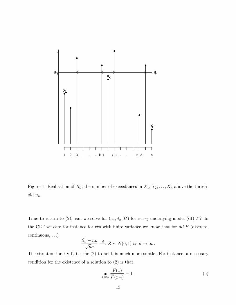
Xn,n = min (X1, . . . , Xn) ≤ Xn−1,n ≤ · · · ≤ X2,n ≤ X1,n = Mn ;

indeed, {Bn = k} = {Xk,n > un, Xk+1,n ≤ un}. Figure 1 gives an example of Bn and suggests

the obvious interpretation of Bn as the number of exceedances above the (typically high)

threshold un.

12

●

●

●

●

●

●

●

●

●

x x x x

1 2 3 . . . k−1 k+1 . . . n−2 n

X1

Xk

Xn

Bn

/\

un

Figure 1: Realisation of Bn, the number of exceedances in X1, X2, . . . , Xn above the thresh-

old un.

Time to return to (2): can we solve for (cn, dn, H) for every underlying model (df) F? In

the CLT we can; for instance for rvs with finite variance we know that for all F (discrete,

continuous, . . .)Sn − nµ√

nσ

d−→ Z ∼ N(0, 1) as n →∞ .

The situation for EVT, i.e. for (2) to hold, is much more subtle. For instance, a necessary

condition for the existence of a solution to (2) is that

limx↑xF

F (x)

F (x−)= 1 . (5)

13

Here F (t−) = lims↑t F (s), the left limit of F in t. In the case of discrete rvs, (5) reduces to

limn→∞

F (n)

F (n− 1)= 1 .

The latter condition does not hold for models like the Poisson, geometric or negative binomial;

see EKM, Examples 3.14-6. In such cases, one has to develop a special EVT. Note that (5)

does not provide a sufficient condition, i.e. there are continuous dfs F for which classical

EVT, in the sense of (2), does not apply. More on this later. At this point it is important to

realise that solving (2) imposes some non–trivial conditions on the underlying model (data).

The solution to (2) forms the content of the next theorem. We first recall that two rvs X

and Y (or their dfs FX , FY ) are of the same type if there exist constants a ∈ R, b > 0 so

that for all x ∈ R, FX(x) = FY

(x−a

b

), i.e. X

d= bY + a.

Theorem 1 (Fisher–Tippett). Suppose that X1, X2, . . . are iid rvs with df F . If there

exist norming constants cn > 0, dn ∈ R and a non–degenerate df H so that (2) holds, then

H must be of the following type:

Hξ(x) =

exp{−(1 + ξx)−1/ξ

}if ξ 6= 0 ,

exp{− exp(−x)} if ξ = 0 ,

(6)

where 1 + ξx > 0. �

Remarks

(i) The dfs Hξ, ξ ∈ R, are referred to as the (generalised) extreme value distributions

(GEV). For ξ > 0 we have the Frechet df, for ξ < 0 the Weibull, and for ξ = 0

the Gumbel or double exponential. For applications to finance, insurance and risk

management, the Frechet case (ξ > 0) is the important one.

(ii) The main theorems from probability theory underlying the mathematics of EVT are

(1) The Convergence to Types Theorem (EKM, Theorem A1.5), yielding the functional

forms of the GEV in (6); (2) Vervaat’s Lemma (EKM, Proposition A1.7) allowing the

construction of norming sequences (cn, dn) through the weak convergence of quantile

14

(inverse) functions, and finally (3) Karamata’s Theory of Regular Variation (EKM,

Section A3) which lies at the heart of many (weak) limit results in probability theory,

including Gnedenko’s Theorem ((13)) below.

(iii) Note that all Hξ’s are continuous explaining why we can write “∀x ∈ R” in (3).

(iv) When (2) holds with H = Hξ as in (6), then we say that the data (the model F )

belong(s) to the maximal domain of attraction of the df Hξ, denoted as F ∈ MDA(Hξ).

(v) Most known models with continuous df F belong to some MDA(Hξ). Some examples

in shorthand are:

– {Pareto, student–t, loggamma, g–and–h(h > 0), . . .} ⊂ MDA(Hξ, ξ > 0);

– {normal, lognormal, exponential, gamma, . . .} ⊂ MDA(H0), and

– {uniform, beta, . . .} ⊂ MDA(Hξ, ξ < 0).

– The so–called log–Pareto dfs F (x) ∼ 1(log x)k , x →∞, do not belong to any of the

MDAs. These dfs are useful for the modelling of very heavy–tailed events like

earthquakes or internet traffic data. A further useful example of a continuous df

not belonging to any of the MDAs is

F (x) ∼ x−1/ξ{1 + a sin(2π log x)} ,

where ξ > 0 and a sufficiently small.

The g–and–h df referred to above corresponds to the df of a rv X = egZ−1g

e12hZ2

for

Z ∼ N(0, 1); it has been used to model operational risk.

(vi) Contrary to the CLT, the norming constants have no easy interpretation in general;

see EKM, Table 3.4.2 and our discussion on MDA (Hξ) for ξ > 0 below. It is useful

to know that for statistical estimation of rare events, their precise analytic form is

of less importance. For instance, for F ∼ EXP(1), cn ≡ 1, dn = log n, whereas

for F ∼ N(0, 1), cn = (2 log n)−1/2, dn =√

2 log n − log(4π)+log log n

2(2 log n)1/2 . Both examples

correspond to the Gumbel case ξ = 0. For F ∼ UNIF(0, 1), one finds cn = n−1, dn ≡ 1

leading to the Weibull case. The for our purposes very important Frechet case (ξ > 0)

is discussed more in detail below; see (13) and further.

15

(vii) For later notational reasons, we define the affine transformations

γn : R → R

x 7→ cnx + dn , cn > 0 , dn ∈ R ,

so that (2) is equivalent with

(γn)−1 (Mn)d−→ H , n →∞ . (7)

Although based on Theorem 1 one can work out a statistical procedure (the block–maxima

method) for rare event estimation, for applications to risk management an equivalent for-

mulation turns out to be more useful. The so–called Peaks Over Theshold (POT) method

concerns the asymptotic approximation of the excess df

Fu(x) = P (X − u ≤ x | X > u) , 0 ≤ x < xF − u . (8)

The key Theorem 2 below involves a new class of dfs, the Generalised Pareto dfs (GPDs):

Gξ(x) =

1− (1 + ξx)−1/ξ if ξ 6= 0 ,

1− e−x if ξ = 0 ,

(9)

where x ≥ 0 if ξ ≥ 0 and 0 ≤ x ≤ −1/ξ if ξ < 0. We also denote Gξ,β(x) := Gξ(x/β) for

β > 0.

Theorem 2 (Pickands–Balkema–de Haan). Suppose that X1, X2, . . . are iid with df F .

Then equivalent are:

(i) F ∈ MDA (Hξ), ξ ∈ R, and

(ii) There exists a measurable function β(·) so that:

limu→xF

sup0≤x<xF−u

∣∣Fu(x)−Gξ,β(u)(x)∣∣ = 0 . (10)

�

16

The practical importance of this theorem should be clear: it allows for the statistical mod-

elling of losses Xi in excess of high thresholds u; see also Figure 1. Very early on (mid

nineties), we tried to convince risk managers that it is absolutely important to model Fu(x)

and not just estimate u = VaRα or ESα = E(X | X > VaRα). Though always quoting

VaRα and ESα would already be much better than today’s practice of just quoting VaR.

As explained in MFE, Chapter 6, Theorem 2 forms the basis of the POT–method for the

estimation of high–quantile events in risk management data. The latter method is based on

the following trivial identity:

F (x) = F (u)F u(x− u) , x ≥ u .

Together with the obvious statistical (empirical) estimator F n(u), for F (x) far in the upper

tail, i.e. for x ≥ u, we obtain the natural (semi–parametric) EVT–based estimator:

(F)∧

n(x) =

N(u)

n

(1 + ξ

x− u

β

)−1/bξ. (11)

Here(β, ξ)

are the Maximum Likelihood Estimators (MLEs) based on the excesses (Xi − u)+,

i = 1, . . . , n, estimated within the GPD model (9). One can show that MLE in this case is

regular for ξ > −1/2; note that examples relevant for QRM typically have ξ > 0. Denoting

VaRα(F ) = F←(α), the α100% quantile of F , we obtain by inversion of (11), the estimator

(VaRα(F ))∧n = u +β

ξ

(((1− α)n

N(u)

)−bξ− 1

). (12)

Here, N(u) = # {1 ≤ i ≤ n : Xi > u} (= Bn in Figure 1), the number of exceedances

above u.

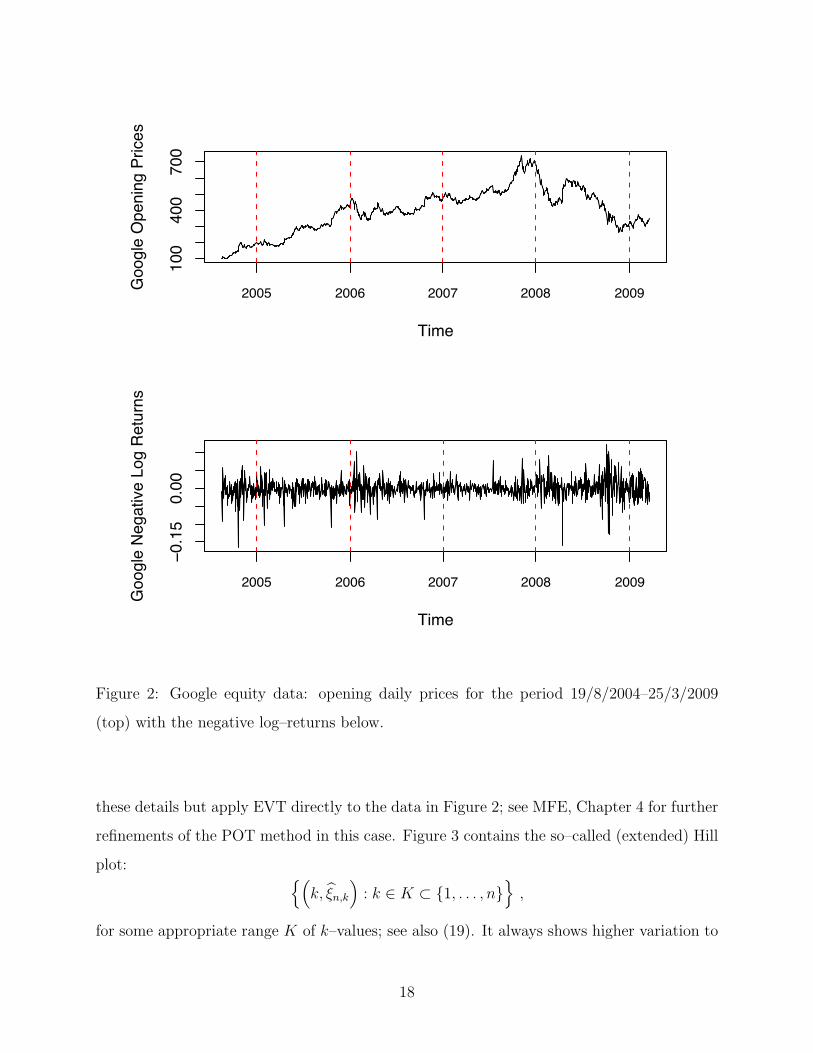
In Figure 2 we have plotted the daily opening prices (top) and the negative log–returns

(bottom) of Google for the period 19/8/2004–25/3/2009. We will apply the POT method

to these data for the estimation of the VaR at 99%, as well as the expected shortfall ESα =

E(X | X > VaRα). It is well known that (log–)return equity data are close to uncorrelated

but are dependent (GARCH or stochastic volatility effects). We will however not enter into

17

10

04

00

70

0

Time

Go

og

le O

pe

nin

g P

rice

s

2005 2006 2007 2008 2009

!0

.15

0.0

0

Time

Go

og

le N

eg

ative

Lo

g R

etu

rns

2005 2006 2007 2008 2009

Figure 2: Google equity data: opening daily prices for the period 19/8/2004–25/3/2009

(top) with the negative log–returns below.

these details but apply EVT directly to the data in Figure 2; see MFE, Chapter 4 for further

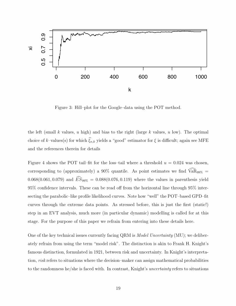
refinements of the POT method in this case. Figure 3 contains the so–called (extended) Hill

plot: {(k, ξn,k

): k ∈ K ⊂ {1, . . . , n}

},

for some appropriate range K of k–values; see also (19). It always shows higher variation to

18

0 200 400 600 800 1000

0.5

0.7

0.9

k

xi

Figure 3: Hill–plot for the Google–data using the POT method.

the left (small k values, u high) and bias to the right (large k values, u low). The optimal

choice of k–values(s) for which ξn,k yields a “good” estimator for ξ is difficult; again see MFE

and the references therein for details

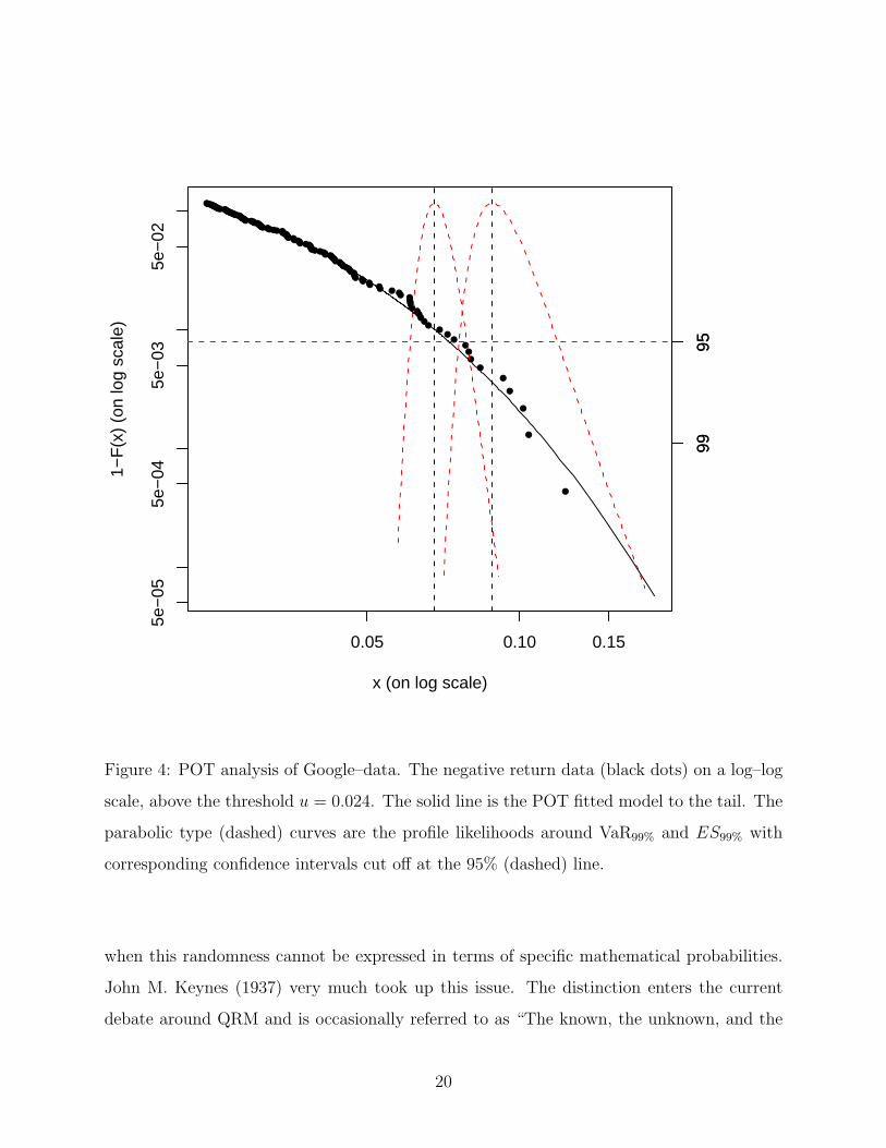
Figure 4 shows the POT tail–fit for the loss–tail where a threshold u = 0.024 was chosen,

corresponding to (approximately) a 90% quantile. As point estimates we find VaR99% =

0.068(0.061, 0.079) and ES99% = 0.088(0.076, 0.119) where the values in parenthesis yield

95% confidence intervals. These can be read off from the horizontal line through 95% inter-

secting the parabolic–like profile likelihood curves. Note how “well” the POT–based GPD–fit

curves through the extreme data points. As stressed before, this is just the first (static!)

step in an EVT analysis, much more (in particular dynamic) modelling is called for at this

stage. For the purpose of this paper we refrain from entering into these details here.

One of the key technical issues currently facing QRM is Model Uncertainty (MU); we deliber-

ately refrain from using the term “model risk”. The distinction is akin to Frank H. Knight’s

famous distinction, formulated in 1921, between risk and uncertainty. In Knight’s interpreta-

tion, risk refers to situations where the decision–maker can assign mathematical probabilities

to the randomness he/she is faced with. In contrast, Knight’s uncertainty refers to situations

19

●●●●●●●●●●●●●●●●●●●●●●●●●●●●●●●●●●●●●●●●●●●●●●●●●●●●●●●●●●●●●●●●●●●●●●●●●●●●●●●●●●●●●●●●●●●●●●●●●●●●●●●●●●● ●● ● ●● ●●●●●●●●●

●●

●●

●●●

●

●

●

●

●

●

0.05 0.10 0.15

5e−

055e

−04

5e−

035e

−02

x (on log scale)

1−F

(x)

(on

log

scal

e)

9995

9995

Figure 4: POT analysis of Google–data. The negative return data (black dots) on a log–log

scale, above the threshold u = 0.024. The solid line is the POT fitted model to the tail. The

parabolic type (dashed) curves are the profile likelihoods around VaR99% and ES99% with

corresponding confidence intervals cut off at the 95% (dashed) line.

when this randomness cannot be expressed in terms of specific mathematical probabilities.

John M. Keynes (1937) very much took up this issue. The distinction enters the current

debate around QRM and is occasionally referred to as “The known, the unknown, and the

20

unknowable.” Stuart Turnbull (personal communication) also refers to dark risk, the risk

we know exists, but we cannot model. Consider the case ξ > 0 in Theorem 2. Besides the

crucial assumption “X1, X2, . . . are iid with df F”, before we can use (10) (and hence (11)

and (12)), we have to understand the precise meaning of F ∈ MDA (Hξ). Any condition with

the df F in it, is a model assumption, and may lead to model uncertainty. It follows from

Gnedenko’s Theorem (Theorem 3.3.7 in EKM) that for ξ > 0, F ∈ MDA (Hξ) is equivalent

to

F (x) = x−1/ξL(x) (13)

where L is a slowly varying function in Karamata’s sense, i.e. L : (0,∞) → (0,∞) measurable

satisfies

∀x > 0 : limt→∞

L(tx)

L(t)= 1 . (14)

Basic notation is L ∈ SV := RV0, whereas (13) is written as F ∈ RV−1/ξ, F is regularly

varying with (tail) index −1/ξ. A similar result holds for ξ < 0. The case ξ = 0 is much

more involved. Note that in the literature on EVT there is no overall common definition

of the index ξ; readers should also be careful when one refers to the tail–index. The latter

can either be ξ, or 1/ξ, or indeed any sign change of these two. Hence always check the

notation used. The innocuous function L has a considerable model uncertainty hidden in its

definition! In a somewhat superficial and suggestive–provocative way, we would even say

MU(EVT) = {L} , (15)

with L as in (13); note that the real (slowly varying) property of L is only revealed at infinity.

The fundamental model assumption fully embodies the notion of power–like behaviour, also

referred to as Pareto–type. A basic model uncertainty in any application of EVT is the slowly

varying function L. In more complicated problems concerning rare event estimation, as one

typically finds in credit risk, the function L may be hidden deep down in the underlying

model assumptions. For instance, the reason why EVT works well for Student–t data but

not so well for g–and–h data (which corresponds to (13) with h = ξ) is entirely due to

the properties of the underlying slowly varying function L. See also Remark (iv) below.

Practitioners (at the quant level in banks) and many EVT–users seem to be totally unaware

of this fact.

21

Like the CLT can be used for statistical estimation related to “average events”, likewise

Theorem 1 can readily be turned into a statistical technique for estimating “rare/extreme

events”. For this to work, one possible approach is to divide the sample of size n into

k(= k(n)) blocks D1, . . . , Dk each of length [n/k]. For each of these data–blocks Di of length

[n/k], the maximum is denoted by M[n/k],i leading to the k maxima observations

M[n/k] ={M[n/k],i, i = 1, . . . , k

}.

We then apply Theorem 1 to the data M[n/k] assuming that (or designing the blocking so

that) the necessary iid assumption is fulfilled. We need the blocksize [n/k] to be sufficiently

large (i.e. k small) in order to have a reasonable approximation to the df of the M[n/k],i,

i = 1, . . . , k through Theorem 1; this reduces bias. On the other hand, we need sufficiently

many maximum observations (i.e. k large) in order to have accurate statistical estimates for

the GEV parameters; this reduces variance. The resulting tradeoff between variance and

bias is typical for all EVT estimation procedures; see also Figure 3. The choice of k = k(n)

crucially depends on L; see EKM, Section 7.1.4, and Remark (iv) and Interludium 1 below

for details.

In order to stress (15) further, we need to understand how important the condition (13)

really is. Gnedenko’s Theorem tells us that (13) is equivalent with F ∈ MDA (Hξ), ξ > 0,

i.e.

∀x > 0 : limt→∞

F (tx)

F (t)= x−1/ξ . (16)

This is a remarkable result in its generality, it is exactly the weak asymptotic condition

of Karamata’s slow variation in (14) that mathematically characterises, though (13), the

heavy–tailed (ξ > 0) models which can be handled, through EVT, for rare event estimation.

Why is this? From Section 3 we learn that the following statements are equivalent:

(i) There exist cn > 0, dn ∈ R : limn→∞ P(

Mn−dn

cn≤ x

)= Hξ(x), x ∈ R, and

(ii) limn→∞ nF (cnx + dn) = − log Hξ(x), x ∈ R.

For ease of notation (this is just a change within the same type) assume that − log Hξ(x) =

x−1/ξ, x > 0. Also assume for the moment that dn ≡ 0 in (ii). Then (ii) with cn = (1/F )←(n)

22

implies that, for x > 0,

limn→∞

F (cnx)

F (cn)= x−1/ξ ,

which is (16) along a subsequence cn → ∞. A further argument is needed to replace the

sequence (cn) by a continuous parameter t in (16). Somewhat more care needs to be taken

when dn 6≡ 0. So F ∈ RV−1/ξ is really fundamental. Also something we learned is that the

norming cn = (1/F )←(n); here, and above, we denote for any monotone function h : R → R,

the generalized inverse of h as

h←(t) = inf{x ∈ R : h(x) ≥ t} .

Therefore, cn can be interpreted as a quantile

P (X1 > cn) = F (cn) ∼ 1

n.

In numerous articles and textbooks, the use and potential misuse of the EVT formulae have

been discussed; see MFE for references or visit www.math.ethz.ch/∼embrechts for a series of

re–/preprints on the topic. In the remarks below and in Interludium 2, we briefly comment on

some of the QRM–relevant pitfalls in using EVT, but more importantly, in asking questions

of the type “calculate a 99.9%, 1 year capital charge”, i.e. “estimate a 1 in 1000 year event”.

Remarks

(i) EVT applies to all kinds of data: heavy–tailed (ξ > 0), medium to short–tailed (ξ = 0),

bounded rvs, i.e. ultra short–tailed (ξ < 0).

(ii) As a statistical (MLE–based) technique, EVT yields (typically wide) confidence in-

tervals for VaR–estimates like in (12). The same holds for PD estimates. See the

Google–data POT analysis, in particular Figure 4, for an example.

(iii) There is no agreed way to choose the “optimal” threshold u in the POT method (or

equivalently k on putting u = Xk,n, see (19) below). At high quantiles, one should

refrain from using automated procedures and also bring judgement into the picture.

We very much realise that this is much more easily said than done, but that is the

nature of the “low probability event”–problem.

23

(iv) The formulae (11) and (12) are based on the asymptotic result (10) as u → xF where

xF = ∞ in the ξ > 0 case, i.e. (13). Typical for EVT, and this contrary to the CLT,

the rate of convergence in (10) very much depends on the second–order properties of

the underlying data model F . For instance, in the case of the Student–t, the rate of

convergence in (10) is O(

1u2

), whereas for the lognormal it is O

(1

log u

)and for the

g–and–h the terribly slow O(

1√log u

). The precise reason for this (e.g. in the ξ > 0

case) depends entirely on the second–order behavior of the slowly varying function L in

(13), hence our summary statement on model uncertainty in (15). Indeed, in the case

of the Student–t, L(x) behaves asymptotically as a constant. For the g–and–h case,

L(x) is asymptotic to exp{(log x)1/2

}/(log x)1/2. As discussed in the Block–Maxima

Ansatz above (choice of k = k(n)) and the rate of convergence (as a function of u) in

the POT method, the asymptotic properties of L are crucial. In Interludium 1 below

we highlight this point in a (hopefully) pedagogically readable way: the EVT end–user

is very much encouraged to try to follow the gist of the argument. Its conclusions hold

true far beyond the example discussed.

(v) Beware of the Hill–horror plots (Hhp); see EKM Figures 4.1.13, 6.4.11 and 5.5.4. The

key messages behind these figures are: (1) the L function can have an important

influence on the EVT estimation of ξ (see also the previous remark); (2) the EVT

estimators for ξ can always be calculated, check relevance first, and (3) check for

dependence in the data before applying EVT. In Interludium 2 below we discuss these

examples in somewhat more detail. Note that in Figure 4.1.13 of EKM, the ordinate

should read as αn.

(vi) We recently came across the so–called Taleb distribution (no doubt motivated by

Taleb [25]). It was defined as a probability distribution in which there is a high prob-

ability of a small gain, and a small probability of a very large loss, which more than

outweighs the gains. Of course, these dfs are standard within EVT and are part of the

GEV–family; see for instance EKM, Section 8.2. This is once more an example where

it pays to have a more careful look at existing, well–established theory (EVT in this

case) rather than going for the newest, vaguely formulated fad.

24

Interludium 1 (L ∈ SV matters!). As already stated above, conditions of the type (13)

are absolutey crucial in all rare event estimations using EVT. In the present interludium we

will high–light this issue based on the Hill estimator for ξ(> 0) in (13). Let us start with the

“easiest” case and suppose that X1, . . . , Xn are iid with df F (x) = x−1/ξ, x ≥ 1. From this

it follows that the rvs Yi = log Xi, i = 1, . . . , n, are iid with df P (Yi > y) = e−y/ξ, y ≥ 0; i.e.

Yi ∼ EXP(1/ξ) so that E (Y1) = ξ. As MLE for ξ we immediately obtain:

ξn = Y n =1

n

n∑i=1

log Xi =1

n

n∑i=1

(log Xi,n − log 1) (17)

where the pedagogic reason for rewriting ξn as in the last equality will become clear below.

Now suppose that we move from the exact Pareto case (with L ≡ 1) to the general case (13);

a natural estimator for ξ can be obtained via Karamata’s Theorem (EKM, Theorem A3.6)

which implies that, assuming (13), we have

limt→∞

1

F (t)

∫ ∞t

(log x− log t) dF (x) = ξ . (18)

(To see this, just use L ≡ 1 and accept that in the end, the SV–property of L allows for the

same limit. These asymptotic integration properties lie at the heart of Karamata’s theory of

regular variation). Replace F in (18) by its empirical estimator Fn(x) = 1n# {i ≤ n : Xi ≤ x}

and put t = Xk,n, the kth order statistic, for some k = k(n) → ∞, this yields in a natural

way the famous Hill estimator for the shape parameter ξ (> 0) in (13):

ξ(H)n,k =

1

k − 1

k−1∑i=1

(log Xi,n − log Xk,n) . (19)

(Compare this estimator with (17) in the case where L ≡ 1). In order to find out how well

EVT–estimation does, we need to investigate the statistical properties of ξ(H)n,k for n → ∞.

Before discussing this point, note the form of the estimator: we average sufficiently many log–

differences of the ordered data above some high enough threshold value Xk,n, the k–th largest

observation. In order to understand now where the problem lies, denote by E1, . . . , En+1 iid

rvs with EXP(1) df, and for k ≤ n + 1 set Γk = E1 + · · · + Ek. Then using the so–called

25

Renyi Representation (EKM, Examples 4.1.10-12) we obtain:

ξ(H)n,k

d= ξ

1

k − 1

k−1∑i=1

Ei +1

k − 1

k−1∑i=1

log

{L (Γn+1/ (Γn+1 − Γn−i+1))

L (Γn+1/ (Γn+1 − Γn−k+1))

}≡ β(1)

n + β(2)n .

(20)

(Hered= denotes “is equal in distribution”). In order to handle β

(1)n we just need k = k(n) →

∞ and use the WLLN, the SLLN and the CLT to obtain all properties one wants (this

corresponds to the L ≡ 1 case above). All the difficulties come from β(2)n where L appears

explicitly. If L is close to a constant (the Student–t case for instance) then β(2)n will go to

zero fast and ξ(H)n,k inherits the very nice properties of the term β

(1)n . If however L is far away

from a constant (like for the loggamma or g–and–h (h > 0)) then β(2)n may tend to zero

arbitrarily slowly! For instance, for L(x) = log x, one can show that β(2)n = O((log n)−1).

Also, in the analysis of β(2)n the various second–order properties of k = k(n) enter. This

has as a consequence that setting a sufficiently high threshold u = Xk,n either in the Block–

Maxima (choice of k) or POT method (choice of u) which is optimal in some sense is very

difficult. Any threshold choice depends on the second–order properties of L! Also note that

the model (13) is semi–parametric in nature: besides the parametric part ξ, there is the

important non–parametric part L.

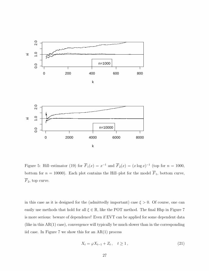
Interludium 2 (Hill–horror plots). The Hhp–phrase mentioned in Remark (v) above

was coined by Sid Resnick and aims at highlighting the difficulties in estimating the shape–

parameter in a model of type (13). The conclusions hold in general when estimating rare

(low probability) events. In Figure 5 we have highlighted the above problem for the two

models F 1(x) = x−1 (lower curve in each panel) and F 2(x) = (x log x)−1, x sufficiently

large, (top curve in each panel). Note that for F2 (i.e. changing from L1 ≡ 1 to L2 =

(log x)−1) interpretation of the Hill–plot is less clear and indeed makes the analysis much

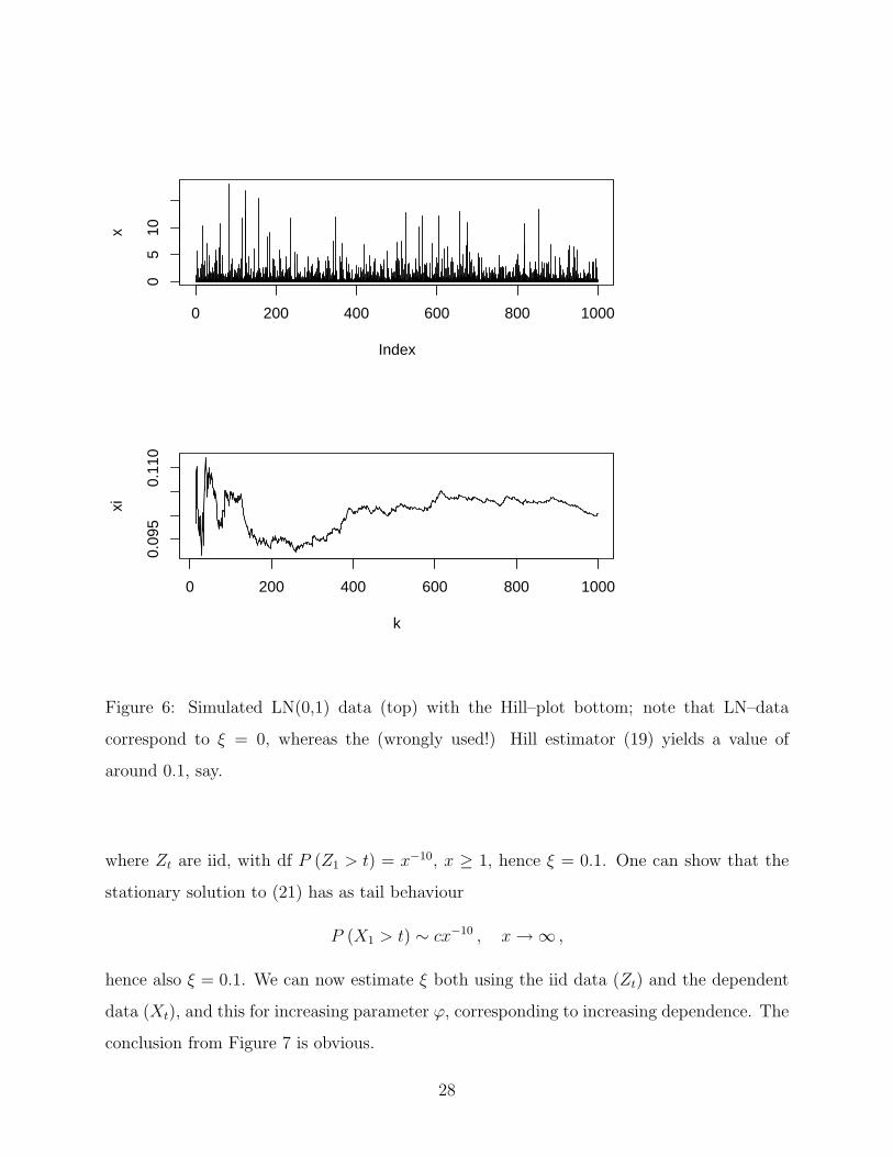
more complicated. In Figure 6 we stress the obvious: apply specific EVT estimators to data

which clearly show the characteristics for which that estimator was designed! For instance,

lognormal data correspond to ξ = 0 and hence the Hill estimator (19) should never be used

26

0 200 400 600 800

0.0

1.0

2.0

k

xi

n=1000

0 2000 4000 6000 8000

0.0

1.0

2.0

k

xi

n=10000

Figure 5: Hill–estimator (19) for F 1(x) = x−1 and F 2(x) = (x log x)−1 (top for n = 1000,

bottom for n = 10000). Each plot contains the Hill–plot for the model F 1, bottom curve,

F 2, top curve.

in this case as it is designed for the (admittedly important) case ξ > 0. Of course, one can

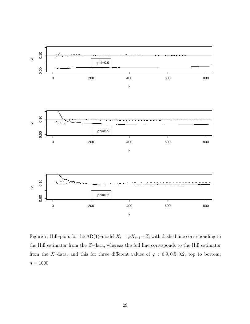
easily use methods that hold for all ξ ∈ R, like the POT method. The final Hhp in Figure 7

is more serious: beware of dependence! Even if EVT can be applied for some dependent data

(like in this AR(1) case), convergence will typically be much slower than in the corresponding

iid case. In Figure 7 we show this for an AR(1) process

Xt = ϕXt−1 + Zt , t ≥ 1 , (21)

27

0 200 400 600 800 1000

05

10

Index

x

0 200 400 600 800 1000

0.09

50.

110

k

xi

Figure 6: Simulated LN(0,1) data (top) with the Hill–plot bottom; note that LN–data

correspond to ξ = 0, whereas the (wrongly used!) Hill estimator (19) yields a value of

around 0.1, say.

where Zt are iid, with df P (Z1 > t) = x−10, x ≥ 1, hence ξ = 0.1. One can show that the

stationary solution to (21) has as tail behaviour

P (X1 > t) ∼ cx−10 , x →∞ ,

hence also ξ = 0.1. We can now estimate ξ both using the iid data (Zt) and the dependent

data (Xt), and this for increasing parameter ϕ, corresponding to increasing dependence. The

conclusion from Figure 7 is obvious.

28

0 200 400 600 800

0.00

0.10

k

xi

phi=0.9

0 200 400 600 800

0.00

0.10

k

xi

phi=0.5

0 200 400 600 800

0.00

0.10

k

xi

phi=0.2

Figure 7: Hill–plots for the AR(1)–model Xt = ϕXt−1+Zt with dashed line corresponding to

the Hill estimator from the Z–data, whereas the full line corresponds to the Hill estimator

from the X–data, and this for three different values of ϕ : 0.9, 0.5, 0.2, top to bottom;

n = 1000.

29

4 MEVT: multivariate extreme value theory

As explained in Section 3, classical one–dimensional extreme value theory (EVT) allows for

the estimation of rare events, such as VaRα for α ≈ 1, but this under very precise model

assumptions. In practice these have to be verified as much as possible. For a discussion

on some practical tools for this, see Chapter 6 in EKM and Chapter 7 in MFE. A critical

view on the possibility for accurate rare event estimation may safeguard the end–user for

excessive model uncertainty (see (15)).

Moving from dimension d = 1 to d ≥ 2 immediately implies that one needs a clear definition

of ordering and what kind of events are termed “extreme”. Several theories exist and are

often tailored to specific applications. So consider n d–variate iid random vectors (rvs) in Rd,

d ≥ 2, X1, . . . , Xn with components Xi = (Xij)j=1,...,d, i = 1, . . . , n. Define the component–

wise maxima

Mnj = max {X1j, X2j, . . . , Xnj} , j = 1, . . . , d ,

resulting in the vector

Mn = (Mn1 , . . . ,Mn

d )′ .

Of course, a realisation m = Mn(ω) need not be an element of the original data X1(ω), . . . , Xn(ω)!

The component–wise version of MEVT now asks for the existence of affine transformations

γn1 , . . . , γn

d and a non–degenerate random vector H, so that

(γn)−1 (Mn) :=((γn

1 )−1 (Mn1 ) , . . . , (γn

d )−1 (Mnd ))′ d→ H , n →∞ ; (22)

see also (7) for the notation used. An immediate consequence from (22) is that the d marginal

components converge, i.e. for all j = 1, . . . , d,(γn

j

)−1 (Mn

j

) d→ Hj , non–degenerate , n →∞ ,

and hence, because of Theorem 1, H1, . . . , Hd are GEVs. In order to characterise the full df

of the vector H we need its d–dimensional (i.e. joint) distribution.

There are several ways in which a characterisation of H can be achieved; they all center

around the fact that one only needs to find all possible dependence functions linking the

30

marginal GEV dfs H1, . . . , Hd to the d–dimensional joint df H. As the GEV dfs are contin-

uous, one knows, through Sklar’s Theorem (MFE, Theorem 5.3), that there exists a unique

df C on [0, 1]d, with uniform–[0, 1] marginals, so that for x = (x1, . . . , xd)′ ∈ Rd,

H(x) = C (H1 (x1) , . . . , Hd (xd)) . (23)

The function C is referred to as an extreme value (EV) copula; its so–called Pickands Repre-

sentation is given in MFE, Theorem 7.45 and Theorem 3 below. Equivalent representations

use as terminology the spectral measure, the Pickands dependence function or the exponent

measure. Most representations are easier to write down if, without loss of generality, one

first transforms the marginal dfs of the data to the unit–Frechet case. Whereas copulae have

become very fashionable for describing dependence (through the representation (23)), the

deeper mathematical theory, for instance using point process theory, concentrates on spectral

and exponent measures. Their estimation eventually allows for the analysis of joint extremal

tail events, a topic of key importance in (credit) risk analysis. Unfortunately, modern MEVT

is not an easy subject to become acquainted with, as a brief browsing through some of the

recent textbooks on the topic clearly reveals; see for instance de Haan and Ferreira [15],

Resnick [23] or the somewhat more accessible Beirlant et al. [7] and Coles [11]. These books

have excellent chapters on MEVT. Some of the technicalities we discussed briefly for the

one–dimensional case compound exponentially in higher dimensions.

In our discussion below, we like to highlight the appearance of, and link between, the various

concepts like copula and spectral measure. In order to make the notation easier, as stated

above, we concentrate on models with unit–Frechet marginals, i.e. for i = 1, . . . , n,

P (Xij ≤ xj) = exp{−x−1

j

}, j = 1, . . . , d , xj > 0 .

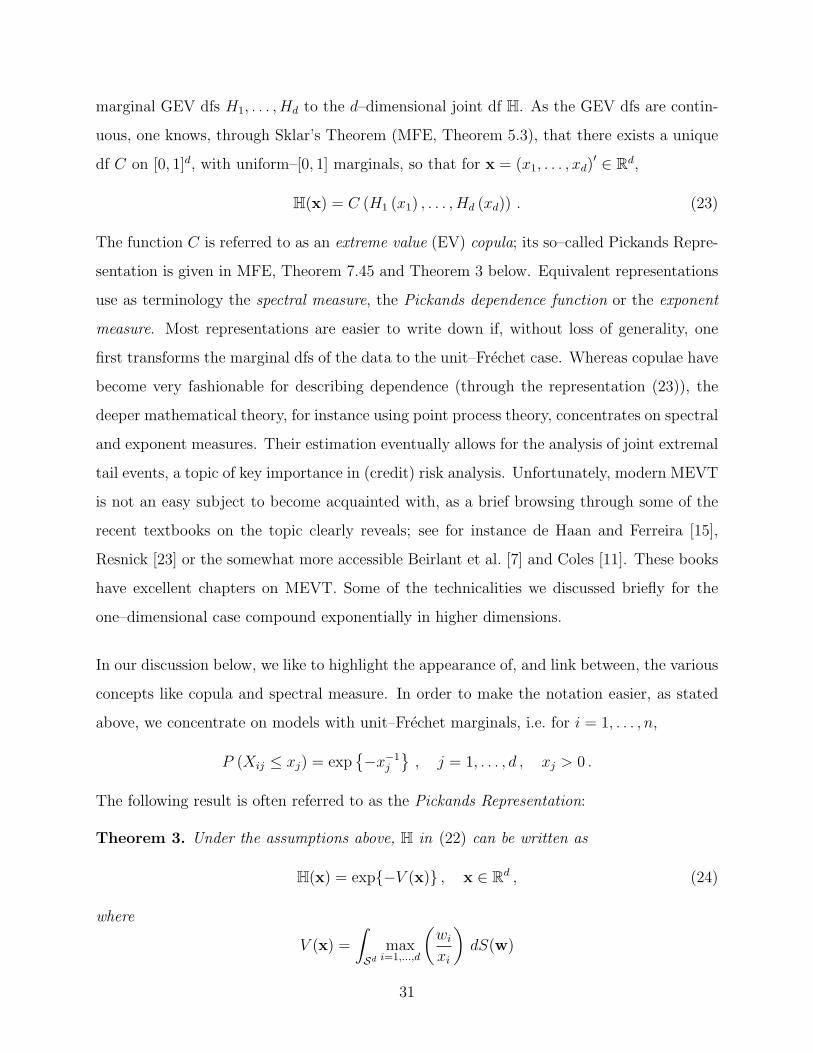
The following result is often referred to as the Pickands Representation:

Theorem 3. Under the assumptions above, H in (22) can be written as

H(x) = exp{−V (x)} , x ∈ Rd , (24)

where

V (x) =

∫Sd

maxi=1,...,d

(wi

xi

)dS(w)

31

and S, the so–called spectral measure, is a finite measure on the d–dimensional simplex

Sd ={x ∈ Rd : x ≥ 0 , ||x|| = 1

}satisfying ∫

Sd

wj dS(w) = 1 , j = 1, . . . , d ,

where || · || denotes any norm on Rd. �

The link to the EVT–copula in (23) goes as follows:

C(u) = exp

{−V

(− 1

log u

)}, u ∈ [0, 1]d . (25)

As a consequence, the function V contains all the information on the dependence between

the d component–wise (limit) maxima in the data. An alternative representation is, for

x ∈ Rd,

V (x) = d

∫Bd−1

max

(w1

x1

, . . . ,wd−1

xd−1

,1−

∑d−1i=1 wi

xd

)dH(w) , (26)

where H is a df on Bd−1 ={x ∈ Rd−1 : x ≥ 0, ||x|| ≤ 1

}, and we have the following norming

∀i = 1, . . . , d− 1 :

∫Bd−1

wi dH(w) =1

d.

Again, H above is referred to as the spectral measure. In order to get a better feeling of

its interpretation, consider the above representation for d = 2, hence B1 = [0, 1] and the

norming constraint becomes: ∫ 1

0

w dH(w) =1

2.

Hence (24) and (26) reduce to

H (x1, x2) = exp

{−2

∫ 1

0

max

(w

x1

,1− w

x2

)dH(w)

}. (27)

Recall that through (24), (26) represents all non–degenerate limit laws for affinely trans-

formed component–wise maxima of iid data with unit–Frechet marginals. The corresponding

copula in (23) takes the form (d = 2, 0 ≤ u1, u2 ≤ 1):

C (u1, u2) = exp

{−2

∫ 1

0

max (−w log u1,−(1− w) log u2) dH(w)

}. (28)

The interpretation of the spectral measure H becomes somewhat clearer through some ex-

amples:

32

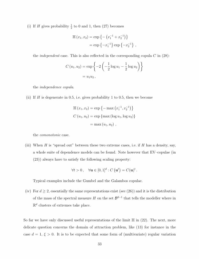
(i) If H gives probability 12

to 0 and 1, then (27) becomes

H (x1, x2) = exp{−(x−1

1 + x−12

)}= exp

{−x−1

1

}exp

{−x−1

2

},

the independent case. This is also reflected in the corresponding copula C in (28):

C (u1, u2) = exp

{−2

(−1

2log u1 −

1

2log u2

)}= u1u2 ,

the independence copula.

(ii) If H is degenerate in 0.5, i.e. gives probability 1 to 0.5, then we become

H (x1, x2) = exp{−max

(x−1

1 , x−12

)}C (u1, u2) = exp {max (log u1, log u2)}

= max (u1, u2) ,

the comonotonic case.

(iii) When H is “spread out” between these two extreme cases, i.e. if H has a density, say,

a whole suite of dependence models can be found. Note however that EV–copulae (in

(23)) always have to satisfy the following scaling property:

∀t > 0 , ∀u ∈ [0, 1]d : C(ut)

= C(u)t .

Typical examples include the Gumbel and the Galambos copulae.

(iv) For d ≥ 2, essentially the same representations exist (see (26)) and it is the distribution

of the mass of the spectral measure H on the set Bd−1 that tells the modeller where in

Rd clusters of extremes take place.

So far we have only discussed useful representations of the limit H in (22). The next, more

delicate question concerns the domain of attraction problem, like (13) for instance in the

case d = 1, ξ > 0. It is to be expected that some form of (multivariate) regular variation

33

will enter in a fundamental way, together with convergence results on (multivariate) Poisson

point processes; this is true and very much forms the content of Resnick [23]. In Section 3

we already stressed that regular variation is the key modelling assumption underlying EVT

estimation for d = 1. The same is true for d ≥ 2; most of the basic results concerning

clustering of extremes, tail dependence, spillover probabilities or contagion are based on

the concept of multivariate regular variation. Below we just give the definition in order

to indicate where the important model assumptions for MEVT applications come from. It

should also prepare the reader for the fact that methodologically “life at the multivariate

edge” is not so simple!

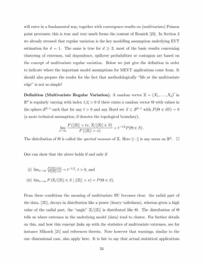
Definition (Multivariate Regular Variation). A random vector X = (X1, . . . , Xd)′ in

Rd is regularly varying with index 1/ξ > 0 if there exists a random vector Θ with values in

the sphere Sd−1 such that for any t > 0 and any Borel set S ⊂ Sd−1 with P (Θ ∈ ∂S) = 0

(a more technical assumption; ∂ denotes the topological boundary),

limx→∞

P (||X|| > tx, X/||X|| ∈ S)

P (||X|| > x)= t−1/ξP (Θ ∈ S) .

The distribution of Θ is called the spectral measure of X. Here || · || is any norm on Rd. �

One can show that the above holds if and only if

(i) limx→∞P (||X||>tx)P (||X||>x)

= t−1/ξ, t > 0, and

(ii) limx→∞ P (X/||X|| ∈ S | ||X|| > x) = P (Θ ∈ S).

From these conditions the meaning of multivariate RV becomes clear: the radial part of

the data, ||X||, decays in distribution like a power (heavy–tailedness), whereas given a high

value of the radial part, the “angle” X/||X|| is distributed like Θ. The distribution of Θ

tells us where extremes in the underlying model (data) tend to cluster. For further details

on this, and how this concept links up with the statistics of multivariate extremes, see for

instance Mikosch [21] and references therein. Note however that warnings, similar to the

one–dimensional case, also apply here. It is fair to say that actual statistical applications

34

of MEVT are often restricted to lower dimensions, d ≤ 3, say; besides Beirlant et al. [7],

see also Coles [11] for a very readable introduction to the statistical analysis of multivariate

extremes. Finally, the statement “Here || · || is any norm in Rd” is very useful for QRM.

Indeed, ||X|| can take several meanings depending on the norm chosen.

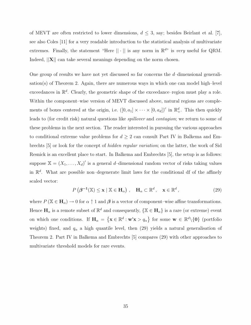
One group of results we have not yet discussed so far concerns the d–dimensional generali-

sation(s) of Theorem 2. Again, there are numerous ways in which one can model high–level

exceedances in Rd. Clearly, the geometric shape of the exceedance–region must play a role.

Within the component–wise version of MEVT discussed above, natural regions are comple-

ments of boxes centered at the origin, i.e. ([0, a1]× · · · × [0, ad])c in Rd

+. This then quickly

leads to (for credit risk) natural questions like spillover and contagion; we return to some of

these problems in the next section. The reader interested in pursuing the various approaches

to conditional extreme value problems for d ≥ 2 can consult Part IV in Balkema and Em-

brechts [5] or look for the concept of hidden regular variation; on the latter, the work of Sid

Resnick is an excellent place to start. In Balkema and Embrechts [5], the setup is as follows:

suppose X = (X1, . . . , Xd)′ is a general d–dimensional random vector of risks taking values

in Rd. What are possible non–degenerate limit laws for the conditional df of the affinely

scaled vector:

P(β−1(X) ≤ x | X ∈ Hα

), Hα ⊂ Rd , x ∈ Rd , (29)

where P (X ∈ Hα) → 0 for α ↑ 1 and β is a vector of component–wise affine transformations.

Hence Hα is a remote subset of Rd and consequently, {X ∈ Hα} is a rare (or extreme) event

on which one conditions. If Hα ={x ∈ Rd : w′x > qα

}for some w ∈ Rd\{0} (portfolio

weights) fixed, and qα a high quantile level, then (29) yields a natural generalisation of

Theorem 2. Part IV in Balkema and Embrechts [5] compares (29) with other approaches to

multivariate threshold models for rare events.

35

5 MEVT: return to credit risk

At present (April 2009), it is impossible to talk about low probability events, extremes and

credit risk, without reflecting on the occasionally very harsh comments made in the (popular)

press against financial engineering (FE). For some, FE or even mathematics is the ultimate

culprit for the current economic crisis. As an example, here are some quotes from the rather

misleading, pamphlet like “The secret formula that destroyed Wall Street” by Felix Salmon

on the Market Movers financial blog at Portfolio.com:

– “How one simple equation (P = Φ(A, B, γ)) made billions for bankers – and nuked

your 401(k) (US pension scheme).”

– “Quants’ methods for minting money worked brilliantly . . . until one of them devastated

the global economy.”

– “People got excited by the formula’s elegance, but the thing never worked. Anything

that relies on correlation is charlatanism.” (Quoted from N. Taleb).

– Etc. . . .

Unfortunately, the pamphlet–like tone is taken over by more serious sources like the Fi-

nancial Times; see “Of couples and copulas” by Sam Jones in its April 24, 2009 edition.

Academia was very well aware of the construction’s Achilles heel and communicated this

on very many occasions. Even in the since 1999 available paper Embrechts et al. [18] we

gave in Figure 1 a Li–model type simulation example showing that the Gaussian copula will

always underestimate joint extremal events. This point was then taken up further in the

paper giving a mathematical proof of this fact; see Section 4.4 in that paper. This result

was published much earlier and well–known to anyone working in EVT; see Sibuya [24].

Note that with respect to this fundamental paper there is some confusion concerning the

publication date: 1959 versus 1960. It should indeed be 1959 (Professor Shibuya, personal

communication). This definitely answers Jones’ question: “Why did no one notice the for-

36

mula’s Achilles heel?”. The far more important question is “Why did no one on Wall Street

listen?”.

The equation referred to above is Li’s Gaussian copula model (see (31)), it also lies at the basis

for the harsh comments in Example 7. Whereas the correlation mentioned enters through the

Gauss, i.e. multivariate normal distribution, in memory of the great Carl Friedrich Gauss, it

would be better to refer to it plainly as the normal copula, i.e. the copula imbedded in the

multivariate normal df. This is also the way David Li referred to it in his original scientific

papers on the pricing of CDOs. The basic idea goes back to the fairly straightforward formula

(23). It is formulae like (23) applied to credit risk which form the basis of Chris Rogers’

comments in Example 10 when he talks of “garbage prices being underpinned by garbage

modelling”. For some mysterious reason, after the “formula” caught the eyes of Wall Street,

many thought (even think today; see quotes above) that a complete new paradigm was born.

Though we have stated the comments below on several occasions before, the current misuse of

copula–technology together with superficial and misleading statements like in Salmon’s blog,

prompt us to repeat the main messages again. As basic background, we refer to Embrechts

[16] and Chavez–Demoulin and Embrechts [9] where further references and examples can be

found. We refrain from precise references for the various statements made below; consult

the above papers for more details and further reading.

First of all, the copula concept in (23) is a trivial (though canonical) way for linking the

joint df H with the marginal dfs H1, . . . , Hd of the d underlying risks X1, . . . , Xd. Its use,

we have always stressed, is important for three reasons: pedagogic, pedagogic, stress–testing.

Note that we do not include pricing and hedging! We emphasise “pedagogic” as the copula

concept is very useful in understanding the inherent weaknesses in using the concept of

(linear) correlation in finance (as well as beyond). For instance, if H is multivariate normal

H ∼ Nd(µ, Σ), with correlations ρij < 1, then for every pair of risks (Xi, Xj) we have that

P(Xj > F−1

j (α) | Xi > F−1i (α)

)→ 0 , α ↑ 1 , (30)

so that Xi and Xj are so–called asymptotically (α ↑ 1) independent. Of course, one could

interpret the high quantiles F−1(α) as VaRα. As a consequence, the multivariate normal

37

is totally unsuited for modelling joint extremes. More importantly, this asymptotic inde-

pendence is inherited by the Gaussian copula CGaΣ underlying Nd(µ, Σ). As a consequence,

every model (including the Li model) of the type

HGaΣ = CGa

Σ (H1, . . . , Hd) (31)

is not able to model joint extremes (think of joint defaults for credit risks) effectively and

this whatever form the marginals H1, . . . , Hd take. It is exactly so–called meta–models of

the type (31) that have to be handled with great care and be avoided for pricing. For

stress–testing static (i.e. non–time dependent) risks they can be useful. Recall that in the

original Li model, H1, . . . , Hd were gamma distributed time–to–default of credit risks and the

covariance parameters Σ were estimated for instance through market data on Credit Default

Swaps (CDS). Upon hearing this construction and calibration, Guus Balkema (personal

communication) reacted by saying that “This has a large component of Baron Munchhausen

in it”; recall the way in which the famous baron “bootstrapped” himself and his horse out

of a swamp by pulling his own hair.

Also note that, in general, there is no standard time–dynamic stochastic process model

linked to the copula construction (23) (or (31)) so that time dependence in formulae like

(31) typically enters through inserting (so–called implied) time dependent parameters. As

the latter are mainly correlations, we again fall in the Munchhausen caveat that correlation

input is used to bypass the weakness of using correlations for modelling joint extremal

behaviour. We will not discuss here the rather special cases of Levy–copulae or dynamic

copula constructions for special Markov processes. For the moment it is wise to consider

copula techniques, for all practical purposes, essentially as static.

Interludium 3 (Meta–models). We briefly want to come back to property (30) and the

copula construction (23). One of the “fudge models” too much in use in credit risk, as well as

insurance risk, concerns so–called meta–models. Take any (for ease of discussion) continuous

marginal risk dfs F1, . . . , Fd, and any copula C, then

F(x) = C (F1 (x1) , . . . , Fd (xd)) (32)

38

always yields a proper df with marginals F1, . . . , Fd. By construction, C “codes” the de-

pendence properties between the marginal rvs Xi(∼ Fi), i = 1, . . . , d. When the copula C

and the marginals Fi “fit together” somehow, then one obtains well–studied models with

many interesting properties. For instance, if F1 = · · · = Fd = N(0, 1) and C is the nor-

mal copula with covariance matrix Σ, then F is a multivariate normal model. Similarly, if

one starts with F1 = · · · = Fd = tν a Student–t distribution on ν degrees of freedom (df)

and C is a t–copula on ν df and covariance matrix Σ, then F is a multivariate Student–t

distribution. As models they are elliptical with many useful properties, for instance, all

linear combinations are of the same (normal, t) type, respectively. The normal model shows

no (asymptotic) tail–dependence (see (30)), whereas the t–model shows tail–dependence,

leading to a non–zero limit in (30). On the other hand, because of elliptical symmetry,

upper (NE) as well as lower (SW) clustering of extremes are the same. These models have

a straightforward generalisation to multivariate processes, the multivariate normal distribu-

tion leading to Brownian motion, the t–model to the theory of Levy processes. If however

C and F1, . . . , Fd in (32) do not fit together within a well–understood joint model, as was

indeed the case with the Li–model used for pricing CDOs, then one runs the danger of ending

up with so–called meta–models which, with respect to extremes, behave in a rather degen-

erate way. A detailed discussion of this issue is to be found in Balkema et al. [6]. In the

language of MFE, the Li–model is a meta-Gaussian model. Putting a t–copula on arbitrary

marginals yields a meta–t model exhibiting both upper as well as lower tail–dependence.

For upper tail–dependence, one can use for instance the Gumbel copula whereas the Clayton

copula exhibits lower tail dependence. A crucial question however remains “which copula

to use?” and more importantly “Should one use a copula construction like (32) at all?” So

called copula–engineering allows for the construction of copulas C which exhibit any kind of

dependence/clustering/shape of the sample clouds in any part of [0, 1]d, however very few of

such models have anything sensible to say on the deeper stochastic nature of the data under

study. We therefore strongly advise against using models of the type (32) for any purpose

beyond stress–testing or fairly straightforward calculations of joint or conditional probabili-

ties. Any serious statistical analysis will have to go beyond (32). If one wants to understand

clustering of extremes (in a non–dynamic way) one has to learn MEVT and the underlying

39

multivariate theory of regular variation: there is no easy road to the land of multivariate

extremism!

We were recently asked by a journalist: “Is there then an EVT–based pricing formula avail-

able or around the corner for credit risk?”. Our clear answer is definitely “No!”. (M)EVT

offers the correct methodology for describing and more importantly understanding (joint)

extremal risks, so far it does not yield a sufficiently rich dynamic theory for handling compli-

cated (i.e. high–dimensional) credit–based structured products. A better understanding of

(M)EVT will no doubt contribute towards a curtailing of over–complicated FE–products for

the simple reason that they are far too complex to be priced and hedged in times of stress.

The theory referred to in this paper is absolutely crucial for understanding these limitations

of Financial Engineering. It helps in a fundamental way the understanding of the inherent

Model Uncertainty (MU again) underlying modern finance and insurance. As a consequence

one has to accept that in the complicated risk landscape created by modern finance, one is

well advised to sail a bit less close to the (risk–)wind. Too many (very costly) mistakes were

made by believing that modern FE would allow for a better understanding and capability of

handling complicated credit products based on rare events, like for instance the AAA rated

senior CDO tranches.

An area of risk management where (M)EVT in general, and copulae more in particular,

can be used in a very constructive way is the field of risk aggregation, concentration and

diversification. We look at the problem from the point of view of the regulator: let X1, . . . , Xd

be d one–period risks so that, given a confidence level α, under the Basel II framework, one

needs to estimate VaRα (X1 + · · ·+ Xd) and compare this to VaRα (X1) + · · ·+ VaRα (Xd).

The following measures are considered:

(M1) D(α) = VaRα

(d∑

k=1

Xk

)−

d∑k=1

VaRα (Xk) , and

(M2) C(α) =VaRα

(∑dk=1 Xk

)∑d

k=1 VaRα (Xk).

Diversification effects are typically measured using D(α) leading to the important question of

sub– versus superadditivity. When C(α) ≤ 1 (coherence!), then C(α)100% is often referred

40

to as a measure of concentration. In the case of operational risk, it typically takes values

in the range 70–90%. Of course, both quantities D(α) and C(α) are equivalent and enter

fundamentally when discussing risk aggregation, or indeed risk allocation. These concepts

are not restricted to Value–at–Risk (VaR) as a risk measure, but they enter the current

regulatory (Basel II) guidelines based on VaR.

A careful analysis of D(α) as well as C(α) now involves all (M)EVT tools discussed above.

Starting from applications of one–dimensional EVT, for estimating the individual VaRα (Xk)–

factors or transform marginals to a unit–Frechet scale, to the use of (M)EVT in order to

understand the model uncertainty in the calculation of VaRα

(∑dk=1 Xk

). Indeed, the latter

can only be calculated/estimated if one has sufficient information on the joint df F of the

underlying risk factors X1, . . . , Xd. In the absence of the latter, only bounds can be given,

coding somehow the MU in the calculation of D(α) and C(α). Numerous papers exist on

this topic; as a start, check the website of the second author for joint papers with Giovanni

Puccetti.

So far, we have restricted attention to what one could refer to as classical (M)EVT, even

if several of the developments (like Balkema and Embrechts [5]) are fairly recent. Non–

classical approaches which are worth investigating further are more to be found on the

statistical/computational front. We expect for the years to come to see further impor-

tant developments on Bayesian analysis for extreme event estimation and also on various

applications of methods from robust statistics, though the latter may sound somewhat coun-

terintuitive. In the optimisation literature, methodology known under the name of robust

optimisation will no doubt become useful. Most of these newer techniques address in one

way or another the key MU–issue. A possible paper to start is Arbenz et al. [3]. On the com-

putational side, for the calculation of rare event probabilities, several numerical integration

techniques may be used, including so–called low–discrepancy sequences also known as Quasi

Monte Carlo methods. Tools which have already been applied in the realm of credit risk

modelling are standard Monte Carlo and especially importance sampling techniques. More

broadly, rare event simulation is becoming a field on its own with applications well beyond

finance and insurance.

41

Suppose X, X1, . . . , Xn are iid, d–dimensional random vectors with df F and density f . For

some measurable set A which is to be interpreted as rare or remote, one wants to calculate

P (X ∈ A) =

∫A

f(x) dx (33)

or more generally, for some measurable function h,

E(h(X)) =

∫Rd

h(x) f(x) dx .

The rareness of A in (33) translates into P (X ∈ A) is sufficiently small, so that standard

Monte Carlo techniques become highly inefficient. One of the standard tools in use through-

out credit risk management is that of importance sampling; we explain the main idea for

d = 1 (and this just for ease of notation); we follow Section 8.5 in MFE.

Suppose θ = E(h(X)) =∫ +∞−∞ h(x)f(x)dx, then the Monte Carlo estimator becomes

θMCn =

1

n

n∑i=1

h (Xi) . (34)

For the importance sampling estimator, one looks for an appropriate density function g so

that for r = f/g,

θ =

∫ +∞

−∞h(x) r(x) g(x) dx = Eg(h(X) r(X)) ,

from which one obtains

θISn =

1

n

n∑i=1

h (Xi) r (Xi) , (35)

based on a sample from the g–distribution. The key task now concerns finding an optimal

importance–sampling density g so that

var(θIS

n

)� var

(θMC

n

).

In the case of light–tailed densities f , the standard technique used is known under the name

exponential tilting. For some t ∈ R, one defines

gt(x) = etx f(x)/MX(t)

where the moment–generating function

MX(t) = E(etX)

=

∫ +∞

−∞etx f(x) dx (36)

42

is assumed to exist (light–tailedness!). The key aim of using gt is that it makes the rare

event, for instance {X ≥ c}, “less rare” under the new density gt. Solving for the optimal

density (tilt) corresponds to solving a saddle–point equation. In the case of heavy–tailed

dfs F , the moment–generating function MX(t) typically is not analytic in t = 0 so that

exponential tilting through gt does not work. At this point EVT becomes useful as indeed g

may be chosen from the family of GEVs; see for instance McLeish [19] for a discussion. The

latter paper contains also the g–and–h and skew–normal dfs as examples relevant for risk

management. See also Asmussen and Glynn [4] for a textbook discussion.

We often are confronted by remarks of the type “why bother about theory as one can just

bootstrap for such rare events”. Here a word of warning is in order: the standard situation

where the usual bootstrap fails (i.e. delivers inconsistent estimators) is exactly in the realm

of very heavy–tailed dfs, maxima or extreme quantiles. Ways to remedy this deficiency have

been found but need to be handled with care (the catchword is m–out–of–n bootstrap). For

a start on this problem, see for instance Angus [2] and Chernick [10]. Not surprisingly, the

theory of regular variation also plays a crucial role here; see Section 6.4 in Resnick [23],

it has the telling title “Why bootstrapping heavy–tailed phenomena is difficult”. In using

simulation technology or numerical integration techniques (as there are quadrature formulae

or quasi Monte Carlo), one should always be aware of the essential difference between light–

tailed and heavy–tailed dfs. For instance, in the case of large deviation methodology (which is

also relevant for the above problems) this translates into the standard theory where Cramer’s

condition is satisfied (see (36)) and the theory where Cramer’s condition does not hold,

often translated into a regular variation condition of the type (13). Not being aware of this

fundamental difference may result in faulty applications of existing theory.

6 Conclusion

Modern risk management in general, and credit risk management more in particular is con-

fronted with serious challenges which bring the analysis of rare events to the forefront. In our

43

paper, we discuss some of these developments with the current financial crisis as an overall

background. Besides giving an overview of some of the basic results in EVT and MEVT, we

also address the wider issue of the use, or as some say, misuse, of mathematics and its role

in the current crisis. We stress that a trivial reduction of the crisis to a “too much use of

mathematics” is misleading at best and dangerous at worst. Risk management is concerned

with technical questions, answers to which in part(!) will have to rely on quantitative tools.

In order to avoid a renewed abuse of mathematics, as it was no doubt the case in the credit

crisis, end–users will have to understand better the conditions, strengths and weaknesses of

the methodology they are working with. We as mathematicians must do better in commu-

nicating our findings to the wider public. Or in the words of Ian Stewart: “It is becoming

increasingly necessary, and important, for mathematicians to engage with the general public

... Our subject is widely misunderstood, and its vital role in today’s society goes mostly

unobserved ... Many mathematicians are now convinced that writing about mathematics is

at least as valuable as writing new mathematics ... In fact, many of us feel that it is pointless

to invent new theorems unless the public gets to hear of them.” The current economic crisis

puts this quote in a rather special perspective.

Acknowledgement

The authors take pleasure in thanking the editors and David Hoaglin for several comments

to an earlier version of the paper.

References

[1] V.V. Acharya and M. Richarson (Eds.) (2009) Restoring Financial Stability. How to

Repair a Failed System. Wiley.

[2] J.E. Angus (1993) Asymptotic theory for bootstrapping the extremes. Communications

in Statistics–Theory and Methods 22, 15–30

44

[3] P. Arbenz, P. Embrechts and G. Puccetti (2009) The AEP algorithm for the fast com-

putation of the distribution of the sum of dependent random variables. Preprint, ETH

Zurich.

[4] S. Asmussen and P.W. Glynn (2007) Stochastic Simulation: Algorithms and Analysis.

Springer.

[5] G. Balkema and P. Embrechts (2007) High Risk Scenarios and Extremes. A geometric

approach. Zurich Lectures in Advanced Mathematics, European Mathematical Society

Publishing House.

[6] G. Balkema, P. Embrechts and N. Lysenko (2009) Meta densities and the shape of their

sample clouds. Preprint, ETH Zurich.

[7] J. Beirlant, Y. Goegebeur, J. Segers and J. Teugels (2005) Statistics of Extremes. Theory

and Applications. Wiley.

[8] C. Bluhm and L. Overbeck (2007) Structured Credit Portfolio Analysis, Baskets &

CDOs. Chapman & Hall/CRC.

[9] V. Chavez–Demoulin and P. Embrechts (2009) Revisiting the edge, ten years on. Com-

munications in Statistics–Theory and Methods, to appear.

[10] M.R. Chernick (2007) Bootstrap Methods: A Guide for Practitioners and Researchers,

2nd Ed., Wiley.

[11] S. Coles (2001) An Introduction to Statistical Modeling of Extreme Values. Springer.

[12] M.G. Crouhy, D. Galai and R. Mark (2001) Risk Management. McGraw Hill.

[13] M.G. Crouhy, R.A. Jarrow and S.M. Turnbull (2008) Insights and analysis of current

events: The subprime credit crisis of 2007. Journal of Derivatives 16(1), 81–110.

[14] J. Danıelsson, P. Embrechts, C. Goodheart, C. Keating, F. Muennich, O. Renault and

H.S. Shin (2005) An academic response to Basel II. Special Paper No 130, Financial

Markets Group, LSE.

45

[15] L. de Haan and A. Ferreira (2006) Extreme Value Theory. An Introduction. Springer.

[16] P. Embrechts (2009) Copulas: a personal view. Journal of Risk and Insurance, to appear.

[17] P. Embrechts, C. Kluppelberg and T. Mikosch (1997) Modelling Extremal Events for

Insurance and Finance. Springer.

[18] P. Embrechts, A. McNeil and D. Straumann (2002) Correlation and dependence in risk

management: properties and pitfalls. In M. Dempster (Ed). Risk Management: Value

at Risk and Beyond. Cambridge University Press, 176–223.

[19] D. McLeish (2008) Bounded relative error importance sampling and rare event simula-

tion. Preprint, University of Waterloo.

[20] A.J. McNeil, R. Frey and P. Embrechts (2005) Quantitative Risk Management: Con-

cepts, Techniques, Tools. Princeton University Press.

[21] T. Mikosch (2004) Modeling dependence and tails of financial time series. In B. Finken-

stadt and H. Rootzen (Eds). Extreme Values in Finance, Telecommunications, and the

Environment. Chapman & Hall/CRC, 185–286.

[22] S.I. Resnick (1987) Extreme Values, Regular Variation, and Point Processes. Springer.

[23] S.I. Resnick (2007) Heavy–Tail Phenomena. Probabilistic and Statistical Modeling.

Springer.

[24] M. Sibuya (1959) Bivariate extreme statistics. Annals of the Institute of Statistical Math-

ematics 11, 195–210.

[25] N.N. Taleb (2007) The Black Swan. The Impact of the Highly Improbable. Penguin

Books.

46