Computer-Aided Design 74 (2016) 1–17

Contents lists available at ScienceDirect

Computer-Aided Design

journal homepage: www.elsevier.com/locate/cad

An evolutionary approach to the extraction of object constructiontrees from 3D point clouds

Pierre-Alain Fayolle a,∗, Alexander Pasko b

a The University of Aizu, Japanb Bournemouth University, United Kingdom

a r t i c l e i n f o

Article history:Received 27 November 2014Accepted 10 January 2016

Keywords:Shape modelingGenetic programmingFittingReverse engineeringConstruction treeFunction Representation

a b s t r a c t

In order to extract a construction tree from a finite set of points sampled on the surface of an object, wepresent an evolutionary algorithm that evolves set-theoretic expressions made of primitives fitted to theinput point-set and modeling operations. To keep relatively simple trees, we use a penalty term in theobjective function optimized by the evolutionary algorithm. We show with experiments successes butalso limitations of this approach.

© 2016 Elsevier Ltd. All rights reserved.

1. Introduction

Reverse engineering can be considered as a process of recon-struction from scanned point clouds of geometric models suitablefor further re-use and modifications. These modifications can beperformed on different levels. The lowest level allows for tweakingof the polygonal mesh vertices or control points of parametric sur-faces. To support a higher level of interaction with reconstructedobjects, obtained models have to be parameterized such that theuser could modify individual parts and the entire logic of theobject construction including its topology. Such a parameterizedmodel reconstruction is required in mechanical engineering, bio-engineering, computer animation and other application areas [1].

Parametric solid models usually consist of geometric featurescomposed using surface patches and a design history tree (or afeature tree) that represents the design intent and the sequenceof operations for making a particular model. It is expected that amodification of any parameter has to be propagated through theentire model and it is automatically rebuilt accordingly. The fea-ture recognition is a reverse engineering approach to generatingfeature-based parametric solids with the feature tree defining the

∗ Corresponding author.E-mail addresses: fayolle@u-aizu.ac.jp (P.-A. Fayolle),

apasko@bournemouth.ac.uk (A. Pasko).

http://dx.doi.org/10.1016/j.cad.2016.01.0010010-4485/© 2016 Elsevier Ltd. All rights reserved.

model rebuilding procedure [2]. In practice, the rebuilding proce-dure using the feature tree can fail or result in an invalid object forsome parameter modifications, which is a known problem of para-metric solid modeling.

An alternative approach to creating parameterized models isconstructive solid modeling based on the Constructive Solid Ge-ometry (CSG) [3] or the Function Representation (FRep) [4]. A con-structive model is represented by a binary (CSG) or n-ary (FRep)construction tree structure with primitive solids at the leaves andoperations at the internal nodes of the tree. For any given point inspace, an evaluation procedure traverses the tree and evaluates abinary point membership predicate (CSG) or a value of a real func-tion (FRep) at this point. Such a model can be fully parameterizedand any changes to the parameters are taken into account duringthe next evaluation inquiry without failure. Although an empty setcan be generated as a result of parameter modifications, it is still avalid model.

We are interested in a reverse engineering procedure that canextract a construction FRep tree froma given input point cloud. Thepoint-cloud is first segmented and primitives from a set of tem-plates are fitted to each subset. A tree structure involving the fittedprimitives and modeling operations is then discovered. The treeextraction is a complex optimization problem. We employ an evo-lutionary approach to solve it. Although evolutionary techniqueshave been already used for data fitting, geometric shapes genera-tion and optimization [5], extraction of a construction tree is a newapplication area for genetic algorithms and genetic programming.

2 P.-A. Fayolle, A. Pasko / Computer-Aided Design 74 (2016) 1–17

Contributions. In this work we present an algorithm to:

• segment an input point-set in several subsets and fit primitivesto each of them;

• combine these fitted primitives bymodeling operations in orderto obtain a constructive model for the input point-set;

• limit the size of the evolved construction tree to allow itsreusability.

2. Related works

The work presented here is at the intersection of differentresearch areas: surface reconstruction from discrete point-sets,reverse engineering of solid models and evolutionary approachesfor the synthesis of shapes.Surface reconstruction from discrete point-sets. The problemof reconstructing a surface from sample points is extensivelydiscussed in the computer graphics and geometric modelingliterature. Recent popular methods for surface reconstructionoften involve fitting implicit surfaces. The reconstruction methodproposed by Muraki [6] consists in fitting blobby models to rangedata. In [7], Hoppe et al. reconstruct a surface by computing asigned distance function. Savchenko et al. [8] and Turk et al. [9]proposed to fit a linear combination of radial basis functions tothe input point-set. Compactly supported radial basis functionswere introduced by Morse et al. [10] to decrease the complexityin time andmemory of the previous methods. In [11], Ohtake et al.glue locally fitted quadrics by applying a partition of unity. In [12,13] the authors recover a characteristic function defining a solidby solving a Poisson equation. Different variations of the MovingLeast Squares methodwere used in [14–16]. In a recent paper [17],the authors compute a smoothed distance function to the surfaceunderlying the point-set by minimizing some energy function. Fora deeper survey of this topic, the reader is referred to the work ofBerger et al. [18]. These methods tend to produce verbose models,containing for example a large number of coefficientswhen splinesare used in addition to the original point-set. These models lacksemantic information and cannot be used for inspection or reuseof the structure of the object in contrary to objects built usingconstructive solid modeling methods.Reverse engineering. The goal of reverse engineering is thecreation of accurate and consistent geometric models from varioustypes of input data including three-dimensional point-clouds [19].The reconstructed model should be a valid solid model, ready toundergo further operations in some interactive modeling system.The problems to be solved include: identifying sharp edges andcreases, segmentation, fitting of patches to subsets, treatmentof blends and providing continuity and smoothness betweenthe patches (see Section 2 in [20]). Another important problemis the creation of geometric models respecting constraints [21](e.g. parallelism of planes, concentricity of spheres and others).One of the first steps (similar to the approach presented here)is a segmentation of the input data. It consists in clustering theoriginal point-set into subsets. After the segmentation, primitivesare associated and fitted to each subset. The final step is thecreation of the solid model. It consists in grouping the fittedprimitives to generate a valid boundary representationmodel [21].

Parameterized models reflecting semantics and logic of theirconstruction are most suitable for further operating on them [1].Feature-based parametric solid models include information onsemantically meaningful parts (geometric features) with theirparameters and a history tree (or a feature tree) representingthe sequence of operations for constructing the model. Reverseengineering history of modeling operations from a sequenceof 3D objects is discussed in [22]. Given as input a series of3D objects, each object is segmented and correspondences are

estimated between consecutive objects. This information is thenused to establish the operations between consecutive objects.Reverse engineering of parametric feature-based solids has beenaddressed for mechanical features [23] and for more generaluser-defined features [2]. Wang et al. present several techniquesfor reconstructing features such as extrusion, sweep, blend andothers [24]. A known problem with parametric solid modeling isthat the rebuilding process using the feature tree can fail or resultin an invalid object for some combination of parameter values.

Constructive solid modeling based on CSG [3] or FRep [4]provides fully parameterized valid models. Fitting preliminarymodeled parameterized FRep templates to point clouds waspresented in [25] as a first step to the automation of thereconstruction of constructive models. A reverse engineeringprocedure that can extract a construction FRep tree from the givenpoint cloud is an open research problem addressed in this paper.Segmentation. A necessary step inmost of the reverse engineeringtechniques is the segmentation of the input point-set. Thereare various techniques available depending on the domainof application, see e.g. the Section 1.1 of [26] for a morecomprehensive survey of existing methods. Common techniquesused in reverse engineering are described in [27,20,28,29] andreferences therein. After the segmentation, we need to fit patchesto each cluster. This fitting step can either be done separately fromthe segmentation step as for example in [27,30,20,31] or be donejointly with the segmentation as in [32,33,26].Boundary representation to CSG conversion. Related to the prob-lem that we are trying to solve is the problem of boundary repre-sentation to CSG conversion. This problem was first investigatedin the two-dimensional case for linear polygons in [34,35]. Later,Shapiro extended the algorithm to handle curved polygons [36].Similar algorithms were adapted to three-dimensional polyhe-dra [37], but they do not work for some types of polyhedra. Forthe three-dimensional case, the problem was solved for solidsbounded by second degree surfaces in [38–41]. These algorithmsmay require some additional half-spaces not available from thesurface faces information or from the segmentation.Evolutionary approaches for shape synthesis and optimization.Evolutionary methods have already been used for geometricshape generation and optimization as in [5]. Hamza and Saitouused a tree-based genetic algorithm to optimize the shape ofCSG solids satisfying some given constraints in [42]. Weiss usedgenetic programming for the structural optimization of CADspecification trees in [43]. Analysis of facade is carried out in [44]by finding a hierarchical decomposition that maximizes somemeasure of symmetry. A genetic algorithm is used as an heuristicfor finding the decomposition optimizing this measure. In reverseengineering, an evolutionary search for numerical parametervalues was applied in [45]. A first attempt to recover constructiontrees frompoint-clouddatawas discussed in [46]. The authors usedstrongly typed genetic programming; leaves consist in primitivesparameters and internal nodes are either algebraic operations,set-operations or primitives selected from a set of candidates.Parsimony is used to control the tree size. In spite of this, the size ofthe generated trees is still large, making the application limited tosimple data-sets. Another problem is that it tries to solve severalindependent tasks at the same time by genetic programming:segmentation, fitting and construction tree extraction. This makesthe approach probably unsuitable for complex objects. Given alist of fitted primitives and an input point-set, the authors of [47]used a genetic algorithm to evolve a linear tree (encoded in anarray) with set-operations in the nodes and the given primitivesin the leaves. While complicated objects cannot be represented bya linear tree in general, it is possible to iterate the algorithm tobuild left heavy trees. The problem is the repetition of primitivesnot used in the solid description.

P.-A. Fayolle, A. Pasko / Computer-Aided Design 74 (2016) 1–17 3

Fig. 1. A graphical illustration of the tree extraction algorithm: (1) The input consists of a set of points sampled on the surface of an object (top row, left); (2) The inputpoint-set is segmented into subsets (or clusters) and a primitive is fitted to each subset (top row, middle); (3) Visualization of the corresponding object (top row, right);(4) Genetic programming is used to evolve a construction tree with the fitted primitives as leaves and operations as internal nodes (bottom row). (For interpretation of thereferences to color in this figure legend, the reader is referred to the web version of this article.)

3. Background

Implicit surfaces, function representation. An implicit surface isa surface representing points with a constant value: {(x, y, z) ∈

R3: f (x, y, z) = 0} of some trivariate function f (see [48] and

references therein). For example, a unit sphere can be representedby the set of points satisfying: 1.0 −

x2 + y2 + z2 = 0.

The Function Representation (FRep) (see [4]) considers not onlythe surface but also the bounded interior given by: {(x, y, z) ∈

R3: f (x, y, z) > 0}. Complex objects can be modeled either

by numerical techniques (such as fitting polynomials or splines)or by applying modeling operations to simpler objects. The set-operations (union, intersection, subtraction, complement) can beimplemented by:

• Min/max [49]:

intersection(S1, S2) := min(fS1 , fS2) (1)union(S1, S2) := max(fS1 , fS2) (2)

complement(S) := −fS (3)subtraction(S1, S2) := intersection(S1, complement(S2)) (4)

where S, S1 and S2 are solid objects and fS , fS1 and fS2 theircorresponding functions.

• R-functions [50,4]:

intersection(S1, S2) := fS1 + fS2 −

f 2S1 + f 2S2 (5)

union(S1, S2) := fS1 + fS2 +

f 2S1 + f 2S2 (6)

complement() is defined as in Eq. (3). And subtraction() isdefined as in Eq. (4) in terms of intersection() (Eq. (5)) andcomplement() (Eq. (3)).

This allows for a constructive representation of objects by aset-theoretic expression or equivalently by a trivariate function.Modifications of Eqs. (5) and (6) allow formodeling blends (smoothtransitions between two surfaces—see Eq. (9) and Fig. 15). Otheravailable operations include all rigid body transformations as wellas non-linear deformations.

4. Overview

The input of the proposed algorithm is a finite point-set S givenby coordinates (x, y, z) of points sampled on the object surfaceby some scanning device and vectors (nx, ny, nz) normal to thesurface at each point (x, y, z) (see Fig. 1, top row, left). If onlythe point coordinates are available, the normal vector field can beestimated by the Principal Component Analysis with propagationof a selected orientation (see the algorithms in Sec. 3.2 and3.3 of [7]and in [51]).

4 P.-A. Fayolle, A. Pasko / Computer-Aided Design 74 (2016) 1–17

Given the finite point-set S of points with normals, the goal isto discover an expression for f (x, y, z) involving primitives (suchas sphere, cylinder, torus and others) and geometric operations(such as union, intersection, subtraction and others). It is assumedthat the zero level-set of the function f (x, y, z) defines anapproximation of the surface from which the input points in Sare sampled (see for example the top row, right picture in Fig. 1).The expression f can also equivalently be seen as a tree withthe corresponding geometric operations in its internal nodes andinstances of primitives in its leaves (see as an example the tree inFig. 1, bottom row).

The main steps of the approach are given in Algorithm 1. Thefirst step is used to determine a list of fitted primitives. For thispurpose, the input point-set is first segmented into subsets andfor each of these subsets a primitive most likely describing thissubset is determined and its parameters are fitted (see the middlepicture in the top row of Fig. 1). Details of this step are given inSection 5.1. At the second step, a list of additional primitives (calledseparating primitives) needed for deriving the final expression iscompiled and added to the list of already fitted primitives (seeSection 5.2). At the final step, given the list of fitted primitivescomputed at the previous steps and the input point-set, we usegenetic programming [52] to evolve a construction tree with thefitted primitives in the leaves and geometric operations in theinternal nodes (see Fig. 1, bottom row). The details of this step aregiven in Section 5.3.

Algorithm 1 Construction tree extraction from a finite point-setRequire: Finite point-set S and list of candidate primitives1: Segmentation of S into clusters and fitting of a primitive to each

cluster2: Computation of separating primitives3: Tree evolution by genetic programming with the fitted and

separating primitives in the leaves and geometric operationsin the internal nodes

For the experiments described in Section 6, the set operations(union, intersection, difference and complement) are used asgeometric operations. Primitives are implemented with implicitsurfaces and operations can be implemented with either min/maxor R-functions (min/max were used in the experiments).

5. Algorithm

5.1. Segmentation and fitting

The first step consists in the segmentation of the input point-set into clusters and fitting of primitives to each of these clusters.During the segmentation of the input point-set, we also needto identify a primitive from a set of candidates, such as plane,sphere, cone and others, and fit its parameters to the points of agiven cluster. We are not directly interested in the clusters, butin the list of fitted primitives describing or approximating each ofthese clusters. For this purpose, we can use the approach basedon RANSAC [53] described in [32] that performs the segmentationand fitting at the same time. Given a finite point-set, the bestfitted plane, sphere, cylinder, cone and torus to the point-set arecomputed using the RANSAC approach. Then the fitted primitivethat best describes the data-set is selected and the correspondingpoints are removed from thepoint-set. In order to determinewhichof the fitted primitives best describes the data, the authors of [32]propose to count the number of points from the input point-set Sthat are on or near the surface of the fitted primitive (see Section4.4 in [32]). These two steps are then repeated until the number ofpoints left in the point-set is below some given threshold.

Table 1Fitted parameter values for the sixdetected planes.

Name nx ny nz d

plane0 0 −1 0 −0.5plane1 0 1 0 −0.5plane2 0 0 −1 0.5plane3 1 0 0 0.5plane4 0 0 1 0.5plane5 −1 0 0 0.5

An alternative approach for fitting primitives chosen from alist of candidate primitives is described in [26]. For each type ofprimitive, its parametersmaximizing an objective function (see Eq.(1) in [26]) are computed. The primitive best describing the data isthen selected among all fitted primitives at this step (see Section 5in [26]) and the corresponding points are removed from the point-set. These two steps are repeated until the number of points left inthe point-set is below some given threshold. The lattermethod hasthe advantage of allowing for a larger and extensible set of possibleprimitives (such as ellipsoid or super-ellipsoid for example) but isslower.

Fig. 2 illustrates the result of the segmentation/fitting by theefficient RANSAC algorithm [32] (left and middle pictures) andthe fitting algorithm discussed in [26] (right picture) both appliedto a set of points sampled on the surface of an object made ofellipsoids. The pictures on the left and middle were obtainedwith two different sets of parameters. The segmentation shownat the left is made of 14 subsets with corresponding primitivesmade of spheres and tori. The segmentation shown in the middlehas 4 subsets made as well of spheres and tori. Compare theseresultswith the segmentation shown at the right obtainedwith thealgorithm from [26] that consists of two subsets each associatedwith an ellipsoid. This approximation of the surface by spheres andtori will result in some visible artifacts on the surface of the objectobtained after the final step of Algorithm 1.

The output of the segmentation and fitting step is a list offitted primitives. In the example of the synthetic cube data-setshown in Fig. 5, the result of the first step is the list of fittedprimitives given in Table 1. While we did not implement it forour experiments, it is possible to improve the fitting results ofthe methods discussed in [32] or [26] by identifying relationsbetweenprimitives (examples of such relations includeparallelismof planes, coaxiality of cylinders, etc.) and re-fitting all primitiveswhile enforcing these relations. This approach is discussed in thework [54].

5.2. Separating primitives

Primitives detected on the surface of an object are not alwayssufficient to describe the object with a constructive approach. It issometimes necessary to introduce additional primitives that do notappear in the segmentation. These are called separating primitivesor separators. The idea of introducing such primitives in order todescribe an object by a CSG expression was introduced by Shapiroand Vossler in [38].

Let us illustrate the idea by an example. The object shownin Fig. 3 cannot be described by a constructive expressionusing only set-theoretic operations and the primitives resultingfrom the segmentation step. The left-most image shows thesegmented input point-set. The image in the middle shows thereconstructed object obtained by our algorithm without usingseparating primitives. Note that the smoothed surface joiningthe front and top planes is not properly retrieved even if it wascorrectly identified in the segmentation, where a cylinder wasfitted to the corresponding point-set. The figure on the right shows

P.-A. Fayolle, A. Pasko / Computer-Aided Design 74 (2016) 1–17 5

Fig. 2. Segmentation/fitting obtained by the efficient RANSAC algorithm [32] (left and middle) and the segmentation algorithm of [26] (right). (For interpretation of thereferences to color in this figure legend, the reader is referred to the web version of this article.)

Fig. 3. An example of using separating primitives. Left: segmented point-set. Middle: reconstructed object without using separating primitives. Right: reconstructed objectusing two additional separating planar half-spaces; the blend (smooth transition) is properly reconstructed. (For interpretation of the references to color in this figure legend,the reader is referred to the web version of this article.)

the reconstructed object obtained by using two additional planarhalf-spaces (plane primitives). Note how the smooth transition iscorrectly reconstructed this time.

We use Algorithm 2 in order to compute the list of potentialseparating primitives. We iterate through all the primitivesidentified during the segmentation step. If the primitive isnot a plane, we retrieve the subset of points on or near thisprimitive’s surface. Then we compute the oriented boundingbox corresponding to this point-set and add all the planes ofthe bounding box to the list of primitives obtained from thesegmentation. If the plane to be added is already present in thelist, we discard it. While it is easier to compute the axis alignedbounding box instead of the oriented bounding box, the formerwillnot work in some cases (for example, consider the object in Fig. 3after some arbitrary rotations).

Algorithm 2 Compute separating primitivesRequire: List of fitted primitives and segmented subsets from

step 11: for each primitive Pi and its corresponding subset Si do2: if Pi is not a plane then3: Compute the oriented bounding box b to Si4: for each face f of b do5: Determine the plane supporting f6: Append it to the list of primitives if it is not already in it7: end for8: end if9: end for

10: Return the list of the original primitives with the additionalseparating primitives

The primary reason for adding these separating half-spaces isto clip some of the primitives fitted to the surface. The example

in Fig. 3 illustrates their use in clipping the cylinder, the topand front planes such that the cylinder smoothly joins the twoplanar surfaces. However, using only separating planes seems tobe limited to cases involving canal surfaces whose sphere centerslie on straight lines. In the other cases, limiting the separatingprimitives to planes can be insufficient. For example, consider theobject obtained from two cylinders and a torus smoothly blendingthese two cylinders, as shown in the leftmost image in Fig. 4. Inthis particular case, using separating planes onlywith the approachdescribed aboveproduces the result illustrated in themiddle imageof Fig. 4. It is not possible to improve on this recovered object. Oneway to resolve the issue is to extend Algorithm 2 by appending tothe list of separating primitives one cylinder for each identifiedtorus. The cylinder radius is given by the torus major radius.Using this extended list of separating primitives, we were able togenerate with Algorithm 1 the object shown in Fig. 4, rightmostimage.

Finally, note that all the additional separating primitives donot need to appear in the final expression evolved by the geneticprogramming step. Only a subset (potentially empty) of them willbe used in the final expression.

5.3. Construction tree extraction with genetic programming

Given the input point-set S and a list of fitted primitivesobtained from the previous steps (see Algorithm 1), we wantto discover an expression with the fitted primitives as terminalsymbols and the geometric operations as function symbols, suchthat the surface of the geometric object defined by the zero-levelset of the evolved expression interpolates or approximates thepoints from S. Primitives are implemented as implicit surfaces.We use the signed distance to the primitive’s boundary if easilycomputable otherwise we compute an approximation as proposed

6 P.-A. Fayolle, A. Pasko / Computer-Aided Design 74 (2016) 1–17

Fig. 4. Left: a test object made of cylinders and a torus. Middle: the best recovered constructive model using separating planes only does not properly describe the originalobject. Right: the best recovered constructive model when separating planes and cylinders are used.

by Taubin: a first order approximation of the distance to the zerolevel of f is given by f /∥∇f ∥ [55]. Geometric operations can beimplemented in terms of min/max or R-functions. The expressioncan be equivalently interpreted as a tree with the fitted primitivesin the leaves and the geometric operations in the internal nodes.

The expression is evolved by genetic programming [52].Specifically, we implemented Algorithm 3. A creature in thepopulation corresponds to an expression with fitted primitives asterminal symbols and geometric operations as function symbols.The set of terminals (leaves in the tree corresponding to theexpression) consists of all the fitted primitives obtained fromthe previous steps of Algorithm 1 (see also details in sub-Sections 5.1 and 5.2). The set of functions (or internal nodes intree representation) consists of geometric operations applied tothe leaves and sub-trees. This set should at least contain the set-operations: union, intersection, subtraction and complement. Inorder to work with solids bounded by implicit surfaces, theseset-operations can be implemented with R-functions or min/max.Other modeling operations are available such as, for example:blending [56], tapering, bending and others. However, they requireadditional arguments that would need to be computed by geneticprogramming, which would make the procedure and the searchmore complicated. We have not worked on this issue and it will bea topic of further investigations.

Algorithm 3 Tree extractionRequire: Finite point-set S and list of fitted primitives1: Let s be the population size2: Let µ be the mutation rate3: Let χ be the crossover rate4: p = InitializeRandomPopulation(s) {Create a random initial

population}5: while Stopping criterion is not satisfied do6: p = Rank(p, S) {Evaluate and sort the current population}7: p′

= [p(1), ..., p(n)] {Save the n best creatures in the nextpopulation}

8: while Length(p′) <= s do9: Select two creatures c1 and c2 from p by tournament

10: c ′

1, c′

2 = Crossover(χ, c1, c2)11: c ′

1 = Mutate(µ, c ′

1)12: c ′

2 = Mutate(µ, c ′

2)13: p′

= Append(p′, c ′

1) {Append c ′

1 and c ′

2 to the newpopulation}

14: p′= Append(p′, c ′

2)15: end while16: p = p′

17: end while

In Algorithm 3 the population is initialized with s random crea-tures. The generation of a random creature uses two parameters:the probability to create a subtree at the given node (set to 0.7 in

the experiments) and the maximum depth for the tree (set to 10in the experiments). A random tree is created by drawing a samplefrom a unit uniform distribution and comparing it with the proba-bility to create a subtree. If the sample value is lower and the max-imum depth has not been reached for the tree, an operation is se-lected at random (each operation has the same probability to beselected), and the procedure is recursively called to generate sub-trees. Otherwise, a primitive is selected at random (each primitivehas the same probability to be selected) and the procedure termi-nates.

In all the experiments described below, we use as a stoppingcriterion a maximum number of iterations of the outer loop. Itis possible to use different criteria that use, for example, themean score of the population and the score of the best creature.The section within lines 8–15 can easily be run in parallel bysplitting the loop among several threads since each computationis independent.Fitness function. From one iteration to the next, we always keepthe best n creatures (we used n = 2 in all our experiments).Ranking the creatures of the current population is done as detailedin Algorithm 4. Given a point-set S, we first compute a raw scorefor each creature c using the following objective function:

E(c, S) :=

Ni=1

(exp(−di(c)2) + exp(−θi(c)2)) − λ size(c) (7)

where:

• xi are the points from the input point-set S,• N is the number of points in the point-set S,• di(c) =

f (xi)ϵd

, with f () is the expression corresponding to thecreature c and ϵd a user defined parameter,

• θi(c) =ArcCos(− ∇f (xi)

∥∇f (xi)∥·n⃗i)

α, with∇f the gradient of the expression

corresponding to the creature c , n⃗i the normal vector to thesurface at the point xi, and α a user defined parameter,

• size(c) the function that counts the number of nodes (internaland leaves) in the tree corresponding to the creature c ,

• λ a user defined parameter.

The goal is to maximize E. This objective function smoothlypenalizes models that disagree with the point-cloud data (in termsof being on or near the points and having a normal agreeingwith the points’ normal). With this objective function, for agiven creature, a point at a distance greater than ϵd

√ln(4) and

at which the angle between the gradient and the point normalis greater than α

√ln(4) would contribute less than 1/2 to the

objective value. The second term in (7) is also required to avoidtrivial solutions (for example an expression evaluating to zeroeverywhere). An alternative approach is to voxelize the input dataand count how many voxels are properly classified with the givenexpression, however it will also increase the computational time.This approach is used, for example, in [57]. We are using equal

P.-A. Fayolle, A. Pasko / Computer-Aided Design 74 (2016) 1–17 7

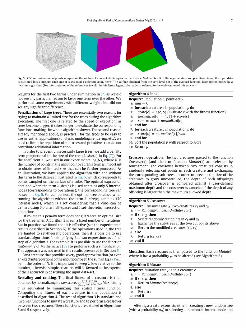
Fig. 5. CSG reconstruction of points sampled on the surface of a cube. Left: Samples on the surface. Middle: Result of the segmentation and primitive fitting; the input datais clustered in six subsets; each subset is assigned a different color. Right: The surface obtained from the zero level-set of the evolved function, here approximated by ameshing algorithm. (For interpretation of the references to color in this figure legend, the reader is referred to the web version of this article.)

weights for the first two terms under summation in (7) as we didnot see any particular reason to favor one term over the other. Weperformed some experiments with different weights but did notsee any significant difference.Penalization of large trees. There are essentially two reasons fortrying to maintain a limited size for the trees during the algorithmexecution. The first one is related to the speed of execution: astrees become bigger, it takes longer to evaluate the correspondingfunctions, making the whole algorithm slower. The second reason,already mentioned above, is practical: for the trees to be easy touse in further applications (analysis, modeling, rendering, etc.), weneed to limit the repetition of sub-trees and primitives that do notcontribute additional information.

In order to prevent unnecessarily large trees, we add a penaltyterm proportional to the size of the tree (λ size(c) in Eq. (7)). Forthe coefficient λ, we used in our experiments log(N), where N isthe number of points in the input point-set. This term is importantto obtain trees of limited size that can be further processed. Asan illustration, we have applied the algorithm with and withoutthis term to the data-set illustrated in Fig. 5, which corresponds topoints sampled on the surface of a cube. The optimal expressionobtained when the term λ size(c) is used contains only 5 internalnodes (corresponding to operations); the corresponding tree canbe seen in Fig. 6. For comparison, the optimal tree obtained whenrunning the algorithm without the term λ size(c) contains 170internal nodes, which is a lot considering that a cube can bedefined using 6 planar half-spaces and 5 set-theoretic intersectionoperations.

Of course this penalty term does not guarantee an optimal sizefor the tree when Algorithm 3 is run a fixed number of iterations.But in practice, we found that it is effective (see the experimentalresults described in Section 6). If the operations used in the treeare limited to set-theoretic operations, then it is possible to usestandard algorithms for simplifying Boolean expressions as a finalstep of Algorithm 3. For example, it is possible to use the functionFullSimplify of Mathematica [58] to perform such a simplification.This approach was not used in the results presented in Section 6.

For a creature that provides a very good approximation (or evenan exact interpolation) of the input point-set, the sum in Eq. (7)willbe in the order of N . It is important to keep λ low relative to thisnumber, otherwise simple creatures will be favored at the expenseof their accuracy in describing the input data-set.Rescaling and ranking. The final fitness of a creature is thenobtained by normalizing its raw score: 1/(1+E(c,s))

c∈p 1/(1+E(c,S)) . MaximizingE is equivalent to minimizing this scaled fitness function.Computing the fitness of each creature in the population isdescribed in Algorithm 4. The rest of Algorithm 3 is standard andinvolves functions to mutate a creature and to perform a crossoverbetween two creatures. These functions are detailed in Algorithms6 and 5 respectively.

Algorithm 4 RankRequire: Population p, point-set S1: sum = 02: for each creature c in population p do3: score[c] = E(c, S) {Evaluate c with the fitness function}4: normalized[c] = 1/(1 + score[c])5: sum = sum + normalized[c]6: end for7: for each creature c in population p do8: score[c] = normalized[c]/sum9: end for

10: Sort the population p with respect to score11: Return p

Crossover operation. The two creatures passed to the functionCrossover() (and then to function Mutate()) are selected bytournament. The crossover between two creatures consists inrandomly selecting cut points in each creature and exchangingthe corresponding sub-trees. In order to prevent the size of thecreatures to grow uncontrolled, the depth of both offspringsobtained after crossover is compared against a user-definedmaximum depth and the crossover is canceled if the depth of anyoffspring is larger than the maximum allowed depth.

Algorithm 5 CrossoverRequire: Crossover rate χ , two creatures c1 and c21: r = RandomNumberInUnitInterval()2: if r < χ then3: Select randomly cut points in c1 and c24: Exchange the sub-trees at the two cut points above5: Return the modified creatures (c1, c2)6: else7: Return (c1, c2)8: end if

Mutation. Each creature is then passed to the function Mutate()where it has a probability µ to be altered (see Algorithm 6).

Algorithm 6MutateRequire: Mutation rate µ and a creature c1: r = RandomNumberInUnitInterval()2: if r < µ then3: Return MutateCreature(c)4: else5: Return c6: end if

Altering a creature consists either in creating a new random tree(with a probabilityµ0) or selecting at random an internal node and

8 P.-A. Fayolle, A. Pasko / Computer-Aided Design 74 (2016) 1–17

0 500 1000 1500 2000 2500 3000iteration

1300

0012

0000

1100

0010

0000

9000

080

000

7000

0

scor

e

Best creature score

Fig. 6. Left: The equivalent tree-based representation of the final expression evolved for the cube. Right: Evolution of the raw fitness function against the number of iterationsof the genetic programming.

replacing the sub-tree with a newly created random sub-tree (seeAlgorithm 7).

Algorithm 7MutateCreatureRequire: Creature c1: r = RandomNumberInUnitInterval()2: if r < µ0 then3: Return a new random tree4: else5: Select randomly a mutation point in c6: Generate a random subtree and attach it at the mutation

point to c7: Return c8: end if

In order to prevent uncontrolled growth of creatures aftermutation, we limit the depth of the newly generated randomsubtree such that the depth of the new creature does not exceedthe user-defined maximal depth.Visualization. The surface approximating the input point-set isgiven by the zero level-set of the best evolved creature f (x, y, z).For visualization purposes, the zero level-set of f can be renderedby techniques such as ray-tracing [59] or approximated bymeshing algorithms (e.g. Marching Cubes based algorithms [60]).It is possible that the zero level-set of the best creature containsextra surfaces not present in the original object. In general,these unnecessary parts are naturally clipped by the otherprimitives during the tree evolution (in particular by the separatingprimitives). In addition, we also compute an object orientedbounding box for the input point-set and take its intersection withthe evolved solid. This prevents unwanted components away fromthe input point-set.

6. Experiments

6.1. Artificial data

6.1.1. Samples on a cubeFirst we test the algorithm against synthetic data. We start

with a simple example consisting of 65000 points sampled onthe surface of a cube. The input data-set is shown in Fig. 5.Segmentation and primitives fitting are first applied to the inputdata. Six subsets are found during the segmentation (see Fig. 5,middle). Each subset corresponds exactly to one of the cube faces.

Segmentation, identification of the most probable primitivesand fitting of their parameters are done jointly. For this particularexample, each cluster is identified as a planar primitive withparameters fitted during the segmentation step. The parametervalues obtained during the fitting are given in Table 1.

Note that in this example, no separating primitives are neededas all segmented subsets correspond to planes. Given the inputpoint-set and the list of fitted primitives, genetic programmingis then used to evolve an expression that combines the fittedprimitives and geometric operations. The final expression is usedto describe the geometry corresponding to the point-set. Thecorresponding surface is obtained as the zero level-set of thisexpression. For this first example, the following expression wasfound by genetic programming:

intersection[plane2, intersection[intersection[subtraction[plane3, union[plane0, plane1]], plane5], plane4]]. (8)

Each primitive is defined by a function of the point coordinates(x, y, z), but the coordinates are removed here for readability. Anequivalent CSG tree for this expression is shown in Fig. 6. The zerolevel-set of the function given by the expression (8) is illustrated inFig. 5, right. It was produced by sampling the function values on athree-dimensional regular grid and approximating the zero level-set with a meshing algorithm.

It is interesting to notice that the expression (8) is minimal.Given six planes, a cube can be defined with five intersections.Another remark is that this evolved expression contains somesubtraction() and union() instead of intersection() operations only.The reason is that not all the planes were fitted with thesame orientation; plane0 and plane1 have, for example, differentorientation than the other planes. The orientations of theseplanes need to be flipped during the evolution of the expressioncorresponding to thewhole object. The following valueswere usedfor the parameters appearing in the fitness function (7): ϵd = 0.01(this value is then scaled by the length of the diagonal of the point-set bounding box) and α = 10°. We used the same values formost of the other experiments. For noisy point-sets alpha wasincreased to 35°. The other parameters of the algorithm are thegenetic programming parameters. The following valueswere used:a mutation rate of 0.3, a crossover rate of 0.3, a population of150 creatures. The initial population of 150 creatures is randomlyinitialized. A large value for the mutation rate is used to preventpremature convergence to a uniform population.

We let Algorithm 3 run for 3000 iterations. The evolution ofthe raw fitness function (the value obtained before population

P.-A. Fayolle, A. Pasko / Computer-Aided Design 74 (2016) 1–17 9

Fig. 7. A tree corresponding to one of the expressions describing the double-torus data-set and extracted by our algorithm.

scaling) for the best creature of the population against the numberof iterations is given in Fig. 6. This data-set is simple enough suchthat after a small number of iterations, the best creature providesalready a correct model for the data; its zero level-set describesthe surface of the cube. This can be seen in the plot in Fig. 6 withthe raw fitness function value for the best creature reaching largevalues early on in the process. The subsequent iterations are spentin trying to find simpler expressions and only contribute a smallimprovement to the raw score.

6.1.2. Double-torusThe second example is a bit more complex, and involves a

larger number of primitives. For this example, 17 408 points (withassociated normals) are sampled on the surface of a double torusobjectmadeof planar parts. In total, eighteen clusters are identifiedand all are recognized correctly as planar surfaces.

One of the expressions discovered by the algorithm resultsin the tree shown in Fig. 7. This tree (and the correspondingexpression) is naturally more complicated than the previousexample. This result was obtainedwith the same parameter valuesas for the precedent example.

Different runs of the algorithm can produce different expres-sions, but their zero level-set should identically describe the inputdata-set. However, the expressions can be different and they mayalso have different contour levels (but identical zero level-set) asillustrated by the contour plots in Fig. 8 of two different expres-sions obtained by two runs of the algorithm for 1000 iterations ona given cross-section (here by the plane y = 0). Here, the contourplots in the left images are similar to the contour plots of the dis-tance to the boundary of the input object. On the other hand, thecontour plots in the right image show that the function value staysalmost constant in the upper right corner. It is not particularly sur-prising that expressions with different level-sets can be obtained,since the constraints that we are trying to enforce control that theinput points are on or near the zero level-set of the evolved ex-pression and that the normals at each points are colinear with thegradient of the expression. In this example, both expressions sat-isfy these criteria. In general, it is preferable toworkwith distance-like fields, such as in the left image of Fig. 8, as the distance to theboundary can be used in further modeling operations [61,62]. Onepossibility to enforce this would be through additional constraints

such as function or gradient values inside or outside the object. Thiswould be at the expense of the runtime speed and it deserves fur-ther investigation. For now, we can notice that the constraints onthe gradient of the expression will guarantee that the function be-haves similarly to the distance function at least close to the bound-ary.

6.2. Scanned and CAD data

6.2.1. Fandisk dataFig. 9 illustrates the results obtained on a more complicated

object. In contrary to the previous examples, this object doesnot involve only planar surfaces. The input point-set and itssegmentation are shown in the top row of Fig. 9. The best CSG treeat the end of 3000 iterations is shown in Fig. 10. The zero level-setof the corresponding expression is approximated with a meshingalgorithm and illustrated in the bottom rowof Fig. 9. The recoveredshape is visually a good approximation of the input point-set (seealso Fig. 19 for log-plots of the error at each point).

Evolution of the raw fitness function value of the best creatureat each iteration of the algorithm is shown in Fig. 11. The earlyjumps in the fitness value are large and contribute mostly tothe final shape of the object. The later jumps are smaller inamplitude and correspond to the improvement of smaller detailsor simplification of the expression while preserving the shapesatisfying the constraints at the input point-set. As shapes becomemore complicated with smaller features and details, it takes alarger number of iterations for the algorithm to converge to anexpression corresponding to a good approximation of the shape.Significant improvements continue to occur in the raw fitnessscore even after a large number of iterations.

6.2.2. Results for additional data-setsResults of the proposed approach applied to additional input

point-sets are shown in Figs. 12 and 13. The point-sets shownin Fig. 12 are obtained by sampling from triangle meshes. Allexpressions were obtained by running the algorithm for 5000iterations with the same parameters as in the precedent examples.The initial population contains 150 random creatures. The sizeof the population is kept unchanged during the iterations. Bothobjects illustrate that reasonably complex shapes can be processedby our algorithm. The recovered object in the bottom row of Fig. 12

10 P.-A. Fayolle, A. Pasko / Computer-Aided Design 74 (2016) 1–17

Fig. 8. Contour plots on a given cross-section (by the plane y = 0) of two expressions obtained by two runs of the algorithm. Top row: visualization of the contour levelswith the surface (corresponding to the zero level-set of the expression) superimposed. Bottom row: visualization of the contour levels on a given cross-section (y = 0) ofthe evolved expressions. (For interpretation of the references to color in this figure legend, the reader is referred to the web version of this article.)

Fig. 9. Top row: Left: Samples on the surface of a fandisk. Right: The segmented point-set with randomly colored subsets. Bottom row: The zero level-set of one of theevolved expressions approximated by a meshing algorithm. (For interpretation of the references to color in this figure legend, the reader is referred to the web version ofthis article.)

also illustrates the effect of the separating primitives with therecovered smooth transition surfaces between the planar surfaces(side) and subtracted cylinders. The behavior of the algorithm onscanned data-sets is also illustrated in Fig. 13. Scanned data cancontain various defects such as noise, flipped normals and others.The algorithm seems to be robust to such defects.

6.3. Applications

The recovered expression or the construction tree can be in-spected and edited in order to perform further modeling oper-ations on the recovered object. Fig. 14 illustrates the contourplots obtained by replacing min/max operations by R-functions

P.-A. Fayolle, A. Pasko / Computer-Aided Design 74 (2016) 1–17 11

Fig. 10. The tree corresponding to one of the solutions discovered by our algorithm.

Fig. 11. Plot of the raw fitness function value against the number of iterations forthe best creature in the population.

[50,4] in the cube expression (8). In general, R-functions or al-ternative implementation of the set-operations [62] are smootherthan min/max, which is a property required for some applicationsor modeling operations such as material distribution modelingin heterogeneous objects [61], blending or metamorphosis oper-ations [56].

To smooth out the creases (sharp features) resulting fromthe surface–surface intersections, it is possible to replace the setoperations by their blending counter-parts [56]. This is illustratedin Fig. 15 for the cube object. The expression was modified byreplacing some of the intersection operations by the blendingintersections.

Specifically, all set operations in (8)were implemented in termsof R-functions (5) and (6) and the intersection operation (5), wasthen replaced by the blending intersection defined by:

blendIntersection(S1, S2, a0, a1, a2)

:= intersection(S1, S2) +a0

1 +f1a1

2+

f2a2

2 . (9)

It is also easy to edit the extracted model by changing some ofthe primitives or the values of someparameters of these primitives.In the example shown in Fig. 16, the expression for the recovereddata-set was modified by doubling the parameter values of theholes (middle image) or the main cylinder (rightmost image).Parameters of extracted expressions can be modified manually bya designer or automatically by some algorithms in order to satisfysome modeling criteria [25,63].

6.4. Computation time

We made a prototype implementation of the algorithmsdescribed in this paper in C++. This implementation is notparticularly optimized for speed. The experiments were run on aregular desktop computer with an Intel Core i3 at 3.30 GHz and4 GB of RAM. The running times for the examples presented inthis paper as well as some additional experimental datasets range

12 P.-A. Fayolle, A. Pasko / Computer-Aided Design 74 (2016) 1–17

Fig. 12. The results of the proposed approach on some CAD parts. For each row, the input, the segmented point-set and the zero level-set of the best expression are shown.(For interpretation of the references to color in this figure legend, the reader is referred to the web version of this article.)

Fig. 13. Results obtained on scanned data with the initial point-sets and the surfaces extracted from the recovered expressions.

Fig. 14. Contour plots of the recovered cube expression when using min/max (left and middle) or R-functions (right) to implement the set-operations. (For interpretationof the references to color in this figure legend, the reader is referred to the web version of this article.)

from dozens of minutes for the simpler shapes to several hoursfor the more complex shapes. Only one thread was used for thecomputation.

The computation time depends essentially on the followingfactors: the complexity of the model, the number of creatures ina population and the number of iterations. The population sizeneeds to be large enough to allow for diversity in the population.In all our experiments, we used 150 creatures per population. Forsimple shapes such as the cube or the double-torus, convergenceis reached quickly as shown by the plots in Fig. 6. Furthermore,since the objects are relatively simple and involve few primitives,

the size of the corresponding trees is small and therefore theevaluation is relatively fast. For complex shapes such as the CADparts or the scanned data, a larger number of iterations is required.The size of the corresponding trees is alsomuch larger. Both factorscontribute to a significantly larger running time for these objects.

There are several techniques that could be used for decreasingthe overall running time. First, it is possible to usemultiple threads,where each thread is responsible for evaluating the objectivefunction (7). Another optimization technique consists in cachingsome of the results. Each primitive’s value and gradient at eachinput point can be precomputed at the beginning and cached. The

P.-A. Fayolle, A. Pasko / Computer-Aided Design 74 (2016) 1–17 13

Fig. 15. Left: original cube object recovered by our approach. Right: the edited cube with some of the set-theoretic operations replaced by their blended counter-parts.

Fig. 16. The zero level-set of a recovered object (left). Edited versions where parameters of some of the primitives were changed: diameter of the holes in the middle imageand diameter of the main cylinder in the right image.

value of the objective function (7) for creatures that are not alteredby mutation or crossover and selected to the next population canbe cached instead of being recomputed.

6.5. Limitations

The limitations of the proposed approach come essentiallyfrom two sources: the segmentation and fitting step and the treeextraction step.Parameters. One limitation of the approach is that it depends onvarious parameters. The fitness function (7) optimized by geneticprogramming contains three parameters: ϵd, α and λ. Additionallythere are the usual parameters of genetic programming: themutation rate, the crossover rate and the size of the population.And finally, there are the parameters related to the segmentationand fitting step (Section 5.1). The parameters of this first stepusually play a similar role to the parameters ϵd and α of thefitness function and are selected based on the quality of the inputpoint-set (presence of noise). Finding appropriate values for theparameter λ required experiments. We found that setting it tolog(N) (N is the number of input points) produced good resultsin all our tests. The genetic programming parameters certainlyhave influence on the convergence of the algorithm. We used theparameter values given in the previous section for all experiments,which gave acceptable results.Fitting. The tree extraction step tries to find a good expressiongiven the list of fitted primitives computed in the precedentsteps. Fitting is usually done within a threshold controlling theaccuracy of fit. This threshold needs to account for noise in theinput data and cannot be too tight. This can result in imprecisionin fitting and under-segmentation (when fitting is used in thesegmentation step). Fig. 17 illustrates the final objects obtainedfrom two different results from the segmentation and fittingstep. For example, in the segmented point-set shown in Fig. 17-left, separate planar surfaces (e.g., the ones in light orange) areidentified as a single cluster and a single primitive is fitted tothe corresponding points instead of two planes (compare the

second and fourth images in Fig. 17). Sometimes parts of objectsare approximated by primitives that do not exactly correspondto the data being described. It results in approximation. See forexample the artificial object in Fig. 2 made of two ellipsoids butapproximated by tori and spheres in the left and middle rows.

The opposite problem occurs when the input data is over-segmented. In this case, the initial data is clustered in lots of subsetsof small size. A large number of primitives are used to match thesesubsets.Tree extraction. A problem of the presented approach is thatsome of the fitted primitives corresponding to surface patchesmay be skipped in the final representation, especially when theycorrespond to small-size features. For example, in the segmenteddata-set shown in Fig. 18 (left), cylinders with small radii arerecognized and fitted to the smooth edges of the object (in yellowand light blue colors), but they are not all used in the recoveredobject in Fig. 18 (right). As we let Algorithm 3 run for only afinite number of time-steps, it is likely that it will finish in aconfiguration that is not a global optimum. As a consequence, someof the features may not be reconstructed correctly. One possibleway to solve this problem is to identify in the input data the pointscorresponding to large values of the recovered expression; thesepoints are then extracted from the input data and Algorithm 1 isrun again on this new point-set. This obtained expression can becombined with the previous expression to improve the result.Approximation. For simple shapes such as the cube shown inFig. 5 or the double-torus, the segmentation and fitting stepproduce accurate results and the tree extraction step generatesminimal accurate expressions. For more complicated shapes, thetree extraction is most likely not going to yield an exact result butrather some approximation. The approximation can be caused byimprecision in fitting (see the discussion above) or it can be causedby extracted expressions that simplify the shape as in Fig. 18.Fig. 19 illustrates the error (log of the error and distribution of theerror) between the extracted expression and the original data-setat each input point. The computed error is an approximation of thedistance between each point and the object surface. It is obtained

14 P.-A. Fayolle, A. Pasko / Computer-Aided Design 74 (2016) 1–17

Fig. 17. Influence of the results of the segmentation/fitting step on the final object. (For interpretation of the references to color in this figure legend, the reader is referredto the web version of this article.)

Fig. 18. A CAD object with smooth edges (blend). The blend are properly identified during the segmentation and cylinders are fitted to them (left). The recovered objectdoes not correctly reconstruct all these features (right). (For interpretation of the references to color in this figure legend, the reader is referred to the web version of thisarticle.)

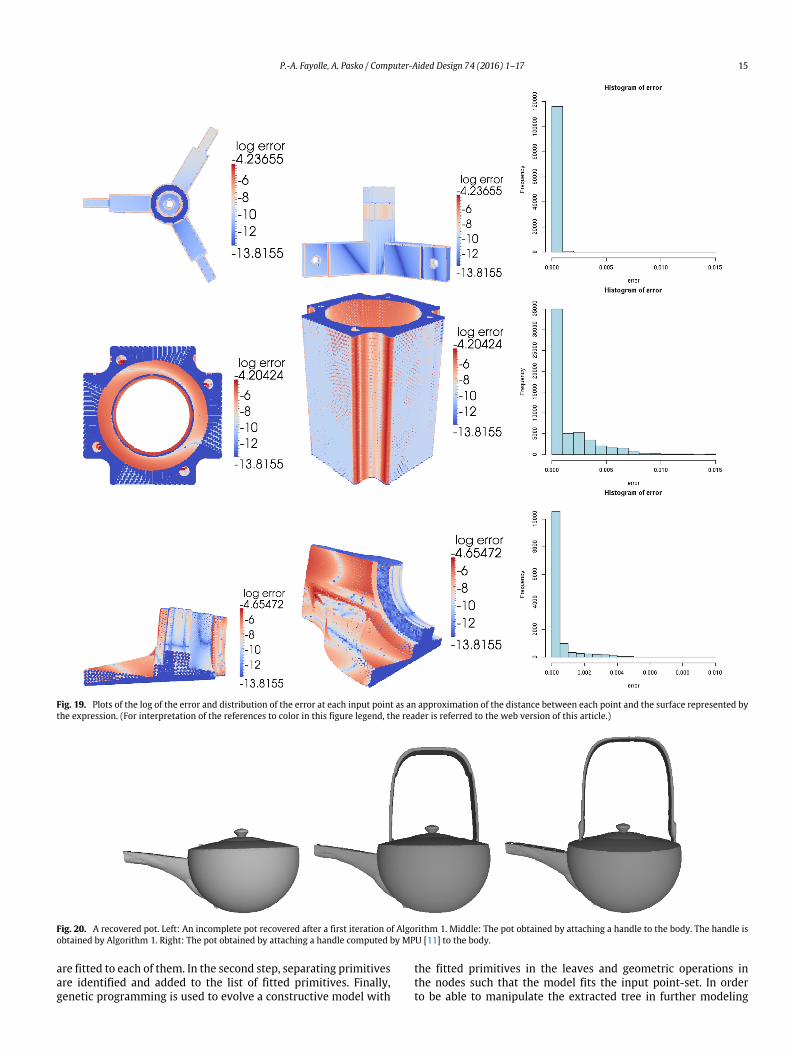
by evaluating the evolved expression at each given point. In orderto make this error independent of the object size, we have dividedeach value by the length of the input point-set bounding box. Thehistograms in the right column illustrate the distribution of theerror.Tree bloat. A common problem found in approaches using geneticprogramming is the creation of bloated trees (large trees withredundant information). In this work, we try to limit the tree sizeby penalizing large trees in the fitness function. This solution seemsto be working for our particular case as can be observed from thevarious trees shown in Figs. 6, 7 or 10 for example. The expressionsgenerated for more complex models seem also to be optimizedwith respect to the tree size, but it is more difficult to verify.However, there is no guarantee that the trees generated by thismethod are optimal and do not contain any redundant informationat all.Additional components. As discussed in Section 5.3, extra surfacepatches can be produced by this approach. However, such parts aregenerally clipped by the other primitives during the tree evolutionand we also clip the final object by the bounding box of the inputpoint-set to remove unwanted components far away. In practice,we did not experience problemswith extra components during ourexperiments. An approach for handling this problemwould consistin penalizing objects with unwanted components during the treegeneration step. It requires an extension of the fitness function (7)with a volumetric term thatwould penalize objectswith unwantedcomponents away from the surface. One possible approach is tocreate a regular grid for the bounding box containing the point-cloud, and classify each cell in this grid with respect to the surfaceunderlying the point-cloud. The classification of each cell can thenbe compared to the object generated by genetic programmingby looking at the sign of its corresponding function at each cell

center. The disadvantage of this approach is that it increases thecomputational time. It also adds new parameters correspondingto the resolution of the grid and its corners. An alternative semi-automatic solution is to incorporate user-interaction in the process(see also the related discussion in Section 6.6 below).

6.6. User-assisted tree extraction

In practice, the loop in Algorithm 3 is executed a finite numberof iterations. Consequently, the best creature obtained at the endmay be incomplete, have some defects or only approximate theinput shape as noted previously. As an example, the pot shown inFig. 20 was incompletely recovered after 3000 iterations (see theleft image). Given the recovered model and the input point-cloud,the set of points corresponding to the handle was automaticallyextracted. Algorithm 1was then iteratively applied on this residualpoint-cloud (the point-cloud corresponding to the handle). The potbody (Fig. 20, left) and the recovered handle were then attachedtogether with the union operation. The final result is shown in themiddle image, Fig. 20.

Some of the smallest components near the bottomof the handleare not completely recovered. In order to obtain the model shownin the right image, Fig. 20, the handle was first reconstructedwith splines (we used MPU [11]) and the handle with its obtainedfunction was then attached to the pot body with the unionoperation.

7. Conclusion

We presented a method for extracting a construction treemodel from an input discrete point-set. First, the point-set issegmented into several subsets and the best describing primitives

P.-A. Fayolle, A. Pasko / Computer-Aided Design 74 (2016) 1–17 15

Fig. 19. Plots of the log of the error and distribution of the error at each input point as an approximation of the distance between each point and the surface represented bythe expression. (For interpretation of the references to color in this figure legend, the reader is referred to the web version of this article.)

Fig. 20. A recovered pot. Left: An incomplete pot recovered after a first iteration of Algorithm 1. Middle: The pot obtained by attaching a handle to the body. The handle isobtained by Algorithm 1. Right: The pot obtained by attaching a handle computed by MPU [11] to the body.

are fitted to each of them. In the second step, separating primitivesare identified and added to the list of fitted primitives. Finally,genetic programming is used to evolve a constructive model with

the fitted primitives in the leaves and geometric operations inthe nodes such that the model fits the input point-set. In orderto be able to manipulate the extracted tree in further modeling

16 P.-A. Fayolle, A. Pasko / Computer-Aided Design 74 (2016) 1–17

operations, we limit the tree size by using a penalty term inthe objective function optimized by genetic programming. Simpleapplications illustrate manipulation of the extracted constructiontree.Future works. The examples used to illustrate our algorithm aremostly man-made parts. One direction of future work is to applythe algorithm to data-sets corresponding to freeform shapes suchas, for example, scanned sculptures. The segmentationprocessmaybe more difficult with more complex primitives to be fitted.

As our algorithm can produce models that do not completelyrecover the surface of the given input point-set (features ordetails missing, for example), it seems important to combine thepresented approach with interactive tools to help the user in thereverse engineering process. A preliminary approach is describedin Section 6.6. However, combining this algorithmwith interactivetools deserves further investigation.

Acknowledgments

The authorswould like to thank the reviewers for their valuablecomments and suggestions. In particular, the example in Fig. 4and the corresponding discussion were suggested by one of thereviewers.

The authors thank the authors of [54] for providing the dataused in their work. This data was used for Fig. 13. The authors alsothank AIM@Shape for providing the data used in Figs. 9, 12 (bottomrow) and 18. Finally, the authors thank E. Kartasheva for providingthe data used for Fig. 12 (top row).

References

[1] Chang K-H, Chen C. 3D shape engineering and design parameterization.Comput-Aided Des Appl 2011;8(5):681–92.

[2] Venkataraman S, Sohoni M, Kulkarni V. A graph-based framework for featurerecognition. In: Sixth ACM symposium on solid modeling and applications.ACM; 2001. p. 194–205.

[3] Requicha A. Representations for rigid solids: theory, methods, and systems.ACM Comput Surv 1980;12(4):437–64.

[4] Pasko A, Adzhiev V, Sourin A, Savchenko V. Function representation ingeometric modeling: concept, implementation and applications. Vis Comput1995;11(8):429–46.

[5] Renner G, editor. Computer-Aided Design, Vol. 35(8). Elsevier; 2003. Specialissue on Genetic Algorithms.

[6] Muraki S. Volumetric shape description of range data using ‘‘blobby model’’.In: Proceedings of SIGGRAPH. 1991. p. 227–35.

[7] Hoppe H, DeRose T, Duchamp T, McDonald J, Stuetzle W. Surface reconstruc-tion from unorganized points. In: SIGGRAPH’92: Proceedings of the 19th an-nual conference on computer graphics and interactive techniques. New York,NY, USA: ACM; 1992. p. 71–8.

[8] Savchenko V, Pasko A, Okunev O, Kunii T. Function representation of solidsreconstructed from scattered surface points and contours. Comput GraphForum 1995;14(4):181–8.

[9] Turk G, OBrien J. Shape transformation using variational implicit functions. In:Proceedings of SIGGRAPH. 1999. p. 335–42.

[10] Morse B, Yoo T, Chen D, Rheingans P, Subramanian K. Interpolating implicitsurfaces from scattered surface data using compactly supported radial basisfunctions. In: Proceedings of shape modeling international. 2001. p. 89–98.

[11] Ohtake Y, Belyaev A, Alexa M, Turk G, Seidel H-P. Multi-level partition of unityimplicits. ACM Trans Graph 2003;22(3):463–70.

[12] Kazhdan M, Bolitho M, Hoppe H. Poisson surface reconstruction. In:Symposium on geometry processing. 2006. p. 61–70.

[13] Kazhdan M, Hoppe H. Screened Poisson surface reconstruction. ACM TransGraph 2013;32(3):29:1–29:13.

[14] Dey TK, Sun J. An adaptive MLS surface for reconstruction with guarantees.In: Proceedings of the third Eurographics symposium on geometry processing.SGP’05. 2005. p. 43–52.

[15] Kolluri R. From range images to 3D models (Ph.D. thesis), The University ofCalifornia at Berkeley; 2005.

[16] Shen C. Building interpolating and approximating implicit surfaces usingmoving least squares (Ph.D. thesis), The University of California at Berkeley;2006.

[17] Calakli F, Taubin G. Ssd: Smoothed signed distance surface reconstruction.Comput Graph Forum 2011;30(7):1993–2002.

[18] Berger M, Levine JA, Nonato LG, Taubin G, Silva CT. A benchmark for surfacereconstruction. ACM Trans Graph 2013;32(2):20:1–20:17.

[19] Varady T, Martin RR, Cox J. Reverse engineering of geometric models-anintroduction. Comput-Aided Des 1997;29(4):255–68.

[20] Benkó P, Martin RR, Várady T. Algorithms for reverse engineering boundaryrepresentation models. Comput-Aided Des 2001;33(11):839–51.

[21] Benkó P, Kós G, Várady T, Andor L, Martin R. Constrained fitting in reverseengineering. Comput Aided Geom Design 2002;19(3):173–205.

[22] Doboš J, Mitra N, Steed A. 3D timeline: Reverse engineering of a part-basedprovenance from consecutive 3D models. Comput Graph Forum 2014;33(2):135–44.

[23] ThompsonWB, Owen JC, de St. Germain Jr HJ, Stark SR, Henderson TC. Feature-based reverse engineering of mechanical parts. IEEE Trans Robot Autom 1999;15(1):57–66.

[24] Wang J, Gu D, Gao Z, Yu Z, Tan C, Zhou L. Feature-based solid modelreconstruction. J Comput Inf Sci Eng 2013;13(1):011004-1–011004-13.

[25] Fayolle P-A, Pasko A, Kartasheva E, Mirenkov N. Shape recovery usingfunctionally represented constructivemodels. In: Proceedings of internationalconference on shapemodeling and applications 2004. SMI’04. 2004. p. 375–78.

[26] Fayolle P-A, Pasko A. Segmentation of discrete point clouds using an extensibleset of templates. Vis Comput 2013;29(5):449–65.

[27] Várady T, Benkó P, Kos G. Reverse engineering regular objects: simplesegmentation and surface fitting procedures. Int J Shape Model 1998;3(4):127–41.

[28] Benkó P, Várady T. Segmentation methods for smooth point regions ofconventional engineering objects. Comput-Aided Des 2004;36(6):511–23.

[29] Várady T, Facello MA, Terék Z. Automatic extraction of surface structures indigital shape reconstruction. Comput-Aided Des 2007;39(5):379–88.

[30] Marshall D, Lukacs G, Martin R. Robust segmentation of primitives from rangedata in the presence of geometric degeneracy. IEEE Trans Pattern Anal MachIntell 2001;23(3):304–14.

[31] Vanco M, Brunnett G. Direct segmentation of algebraic models for reverseengineering. Computing 2004;72(1):207–20.

[32] Schnabel R, Wahl R, Klein R. Efficient ransac for point-cloud shape detection.Comput Graph Forum 2007;26(2):214–26.

[33] Attene M, Falcidieno B, Spagnuolo M. Hierarchical mesh segmentation basedon fitting primitives. Vis Comput 2006;22(3):181–93.

[34] Rvachev VL, Kurpa LV, Sklepus NG, Uchishvili LA. Method of R-functions inproblems on bending and vibrations of plates of complex shape. NaukovaDumka; 1973. p. 121. (in Russian).

[35] Batchelor BG. Hierarchical shape description based upon convex hulls ofconcavities. J Cybern 1980;10:205–10.

[36] Shapiro V. A convex deficiency tree algorithm for curved polygons. Internat JComput Geom Appl 2001;11(2):215–38.

[37] Woo TC. Feature extraction by volume decomposition. In: Proc. conferenceon CAD/CAM technology in mechanical engineering. Cambridge, MA. 1982. p.39–45.

[38] Shapiro V, Vossler DL. Separation for boundary to CSG conversion. ACM TransGraph 1993;12(1):35–55.

[39] Buchele S. Three-dimensional binary space partitioning tree and constructivesolid geometry tree construction from algebraic boundary representations(Ph.D. thesis), The University of Texas at Austin; 1999.

[40] Buchele S, Roles A. Binary space partition tree and constructive solid geometrytree representation for objects bounded by curved surfaces. In: Proceedingsof the thirteenth Canadian conference on computational geometry. 2001. p.49–52.

[41] Buchele SF, Crawford RH. Three-dimensional halfspace constructive solidgeometry tree construction from implicit boundary representations. Comput-Aided Des 2004;36(11):1063–73.

[42] Hamza K, Saitou K. Optimization of constructive solid geometry via a tree-based multi-objective genetic algorithm. In: Proceedings of GECCO. 2004. p.981–92.

[43] Weiss D. Geometry-based structural optimization on CAD specification trees(Ph.D. thesis), ETH Zurich; 2009.

[44] Zhang H, Xu K, JiangW, Lin J, Cohen-Or D, Chen B. Layered analysis of irregularfacades via symmetry maximization. ACM Trans Graph 2013;32(4):121.

[45] Fisher RB. Applying knowledge to reverse engineering problems. Comput-Aided Des 2004;36(6):501–10.

[46] Silva S, Fayolle P-A, Vincent J, PauronG, Rosenberger C, Toinard C. Evolutionarycomputation approaches for shape modelling and fitting. In: Progress inartificial intelligence. Berlin, Heidelberg: Springer; 2005. p. 144–55.

[47] Fayolle P-A, Pasko A, Kartasheva E, Rosenberger C, Toinard C. Automation ofthe volumetric models construction. In: Heterogeneous objectsmodelling andapplications. Berlin, Heidelberg: Springer; 2008. p. 214–38.

[48] Bloomenthal J, Bajaj C, Blinn J, Cani-Gascuel M-P, Rockwood A, Wyvill B,Wyvill G. Introduction to implicit surfaces. Morgan-Kaufmann; 1997.

[49] Ricci A. A constructive geometry for computer graphics. Comput J 1973;16(2):157–60.

[50] Shapiro V. Theory of R-functions and applications: A primer. Technical report.Cornell University; 1988.

[51] Mitra NJ, Nguyen A, Guibas L. Estimating surface normals in noisy point clouddata. Internat J Comput Geom Appl 2004;14(4–5):261–76.

[52] Koza J. Genetic programming. MIT Press; 1992.[53] Fischler MA, Bolles RC. Random sample consensus: a paradigm for model

fitting with applications to image analysis and automated cartography.Commun ACM 1981;24(6):381–95.

[54] Li Y, Wu X, Chrysathou Y, Sharf A, Cohen-Or D, Mitra N. Globfit: Consistentlyfitting primitives by discovering global relations. ACM Trans Graph 2011;30(4):52:1–52:12.

P.-A. Fayolle, A. Pasko / Computer-Aided Design 74 (2016) 1–17 17

[55] Taubin G. Distance approximation for rasterizing implicit curves. ACM TransGraph 1994;13(1):3–42.

[56] Pasko A, Savchenko V. Blending operations for the functionally basedconstructive geometry. In: Set-theoretic solid modeling: techniques andapplications, CSG 94 conference proceedings. Information geometers. 1994.p. 151–61.

[57] Xiao J, Furukawa Y. Reconstructing theworldmuseums. Int J Comput Vis 2014;1–16.

[58] Wolfram Research. Mathematica 7.0. 2008.[59] Hart J. Sphere tracing: A geometric method for the antialiased ray tracing of

implicit surfaces. Vis Comput 1996;12(10):527–45.

[60] Lorensen WE, Cline HE. Marching cubes: a high presolution 3D surfaceconstruction algorithm. Comput Graph 1987;21(4):163–9. Proceedings ofSIGGRAPH 87.

[61] Biswas A, Shapiro V, Tsukanov I. Heterogeneous material modeling withdistance fields. Comput Aided Geom Design 2004;21(3):215–42.

[62] Fayolle P-A, Pasko A, Schmitt B, Mirenkov N. Constructive heterogeneousobject modeling using signed approximate real distance functions. J ComputInf Sci Eng Trans ASME 2006;6(3):221–9.

[63] Chen J, Shapiro V, Suresh K, Tsukanov I. Shape optimization with topologicalchanges and parametric control. Internat J Numer Methods Engrg 2007;71(3):313–46.