Embed Size (px)
Citation preview

AN EVALUATION OF THE EFFECT OF BLAST-GENERATED FRAGMENT SIZE
DISTRIBUTION ON THE UNIT COSTS OF A MINING OPERATION, USING
MODELING AND SIMULATION TECHNIQUES
by
Solomon Augustine Tucker
A dissertation submitted to the faculty of The University of Utah
in partial fulfillment of the requirements for the degree of
Doctor of Philosophy
Department of Mining Engineering
The University of Utah
May 2015

Copyright © Solomon Augustine Tucker 2015
All Rights Reserved

The U n i v e r s i t y of Ut a h G r a d u a t e S c h o o l
STATEMENT OF DISSERTATION APPROVAL
The dissertation of Solomon Augustine Tucker
has been approved by the following supervisory committee members:
Michael K. McCarter Chair 12/19/2014Date Approved
Michael G. Nelson Member 12/19/2014Date Approved
Thomas A. Hethmon Member 12/19/2014Date Approved
Hyung Min Park Member 12/19/2014Date Approved
Raj K. Rajamani Member 12/19/2014Date Approved
and by Michael G. Nelson Chair of
the Department of ________________ Mining Engineering
and by David B. Kieda, Dean of The Graduate School.
ABSTRACT
This research was undertaken to investigate the impacts of finer rock fragmentation
(arising from higher energy blasting) on the unit costs of a hard-rock surface mine. The
investigation was carried out at a copper operation in southern Utah, which exploits its
deposits by conventional methods, including drilling, blasting, loading, and truck
haulage. The run of mine is processed in a three-stage crushing circuit and a two-stage
grinding circuit, which feed a flotation plant that produces a copper concentrate.
The research was carried out using modeling and simulation techniques. Fifty-five
blast designs in total were developed for ore and waste units, with energy inputs ranging
from 100 kcal/st to 400 kcal/st. For each design, fragmentation was predicted using the
Kuz-Ram method. Crushing of the predicted ore fragment size distributions was
simulated using MODSIM™.
Data from pit face imaging and timed motion studies were collected and analyzed for
the influence of fragmentation on shovel and truck productivity. Analyses indicated that
fragment size distribution alone does not significantly impact this productivity.
From simulation of the crushing circuit, it was found that the impact of differences in
the blast-generated fragment distribution on the crusher energy is limited to the primary
crusher, where a vast range of feed size distributions are introduced. No such
relationships were evident at the secondary and tertiary crushers. Energy savings from

increasing blasting intensity proved negligible and would not justify the costs of higher
energy blasting.
There was no evidence from this work that any beneficial influences of blast
generated fragment size distribution reach the grinding mill.
Costs were estimated for drilling, blasting, and crushing, which were the principal
unit operations inferred to be affected in some meaningful way by the varying intensities
of blast energy input.
The research shows that, principally as a result of jaw crusher gape restrictions and
the significant unit costs of secondary reduction for both ore and waste, the net of all
breakage (primary blast, secondary reduction, and crushing) does reduce to a transient
minimum before they begin to ramp up again, thus fitting a classical mine-to-mill curve.
iv

To Yie and Papa
TABLE OF CONTENTS
ABSTRACT............................................................................................................................ iii
ACKNOWLEDGEMENTS.................................................................................................. x
CHAPTERS
1. INTRODUCTION........................................................................................................... 1
1.1 Problem statement..................................................................................................... 11.2 Hypothesis.................................................................................................................. 21.3 Objectives of the research........................................................................................ 31.4 Description of the host operation............................................................................ 41.5 Scope of the research .............................................................................................. 51.6 Units of measure........................................................................................................ 6
2. UNDERSTANDING MINE-TO-MILL PROCESS OPTIMIZATION................... 8
2.1 Overview of mine-to-mill process optimization................................................... 82.2 Evolution of mine-to-mill......................................................................................... 92.3 “Optimum blasting” not based on cost a lo n e ....................................................... 112.4 How blasting influences fragmentation and filters into mine-to-mill............... 122.5 The focus of this research......................................................................................... 13
3. PRINCIPLES FOR THE DESIGN, MEASUREMENT, MODELING, AND SIMULATION OF BLAST FRAGMENTATION..................................................... 18
3.1 Introduction................................................................................................................ 183.2 Blast design objectives, fundamentals, and m ethods.......................................... 18
3.2.1 The objectives and fundamentals of blast design..................................... 183.2.2 The methods of blast design........................................................................ 193.2.3 The Blast Dynamics Energy method......................................................... 22
3.3 Description and modeling of blast fragmentation................................................. 233.3.1 An objective description of the degree of fragmentation........................ 243.3.2 The modeling of particle size distribution................................................ 26
3.4 The measurement and estimation of blast fragmentation.................................... 283.4.1 Photographic granulometry methods......................................................... 28

3.5 The prediction of blast fragmentation.................................................................... .303.5.1 Ouchterlony’s review................................................................................... .31
3.6 The Kuz-Ram model................................................................................................. .323.6.1 The Kuznetsov equation.............................................................................. .333.6.2 Adoption of the Rosin-Rammler equation................................................ .363.6.3 The Uniformity equation............................................................................. .37
3.7 Important limitations to the original Kuz-Ram model......................................... .393.7.1 Important changes to the algorithm........................................................... .39
4. PRINCIPLES, TRENDS, AND METHODS FOR COMMINUTION MODELING AND THE SIMULATION OF CRUSHING SYSTEMS.......................................... 46
4.1 Overview......................................................................................................................464.2 The discussion and reporting of grinding simulation........................................... .464.3 The simulation of mineral processing circuits........................................................47
4.3.1 The Bond model........................................................................................... .484.3.2 Justification for the use of modeling and simulation in this research... 49
4.4 The modeling and simulation of crushing systems............................................... 504.4.1 The jaw crusher model..................................................................................514.4.2 The cone crusher model................................................................................514.4.3 Estimation of crusher classification and breakage functions................. .554.4.4 Estimating the crusher work index..............................................................56
5. FRAGMENTATION MODELING PARAMETERS, BLAST DESIGNS, AND FRAGMENTATION PREDICTION............................................................................ 58
5.1 Overview..................................................................................................................... 585.2 Determination of rock factor, A .............................................................................. 58
5.2.1 Sample collection and preparation............................................................. ..595.2.2 Testing..............................................................................................................615.2.3 Computation of rock factor, A ......................................................................63
5.3 Blast design................................................................................................................ ..635.3.1 Details of blast design.................................................................................. 64
5.4 Prediction of blast fragmentation............................................................................ 64
6. ESTIMATION OF CRUSHER SIMULATION PARAMETERS............................ 83
6.1 Overview..................................................................................................................836.2 Estimation of crushing simulation parameters...................................................... ..83
6.2.1 Preliminaries for parameter estimation..................................................... ..846.2.2 Crusher and screen settings and characteristics....................................... ..866.2.3 The crusher breakage and classification functions.................................. ..866.2.4 The crusher work index............................................................................... ..876.2.5 Verification of crushing simulation parameters....................................... ..88
vii
7. SIMULATION OF THE CRUSHING OPERATION................................................ 99
7.1 Overview..................................................................................................................... 997.2 Simulation setup........................................................................................................ 99
7.2.1 Results............................................................................................................ 1017.2.2 Performance evaluation criteria.................................................................. 1017.2.3 Conclusions about the impact on crushing............................................... 103
8. THE INFLUENCE OF FRAGMENTATION ON DRILLING AND BLASTING COSTS AND LOADING AND HAULING PRODUCTIVITY.............................. 111
8.1 Overview..................................................................................................................... 1118.2 Oversize rock and its implications for secondary breakage and overall costs ...1118.3 The effect of the degree of fragmentation on the costs of drilling and blasting 1128.4 Estimation of the costs of drilling and blasting..................................................... 112
8.4.1 Drilling costs................................................................................................. .1138.4.2 Blasting costs................................................................................................ .114
8.5 The influence of fragment particle size distribution on loading productivity... 1168.6 Evaluation of the loader cycle/productivity versus fragment size distributions 1178.7 Results of statistical analysis................................................................................... .1188.8 Implications................................................................................................................ .1208.9 Estimation of wear and tear arising from degrees of rock fragmentation......... .121
9. THE RELATIONSHIP OF BLAST-GENERATED FRAGMENT SIZE DISTRIBUTION AND UNIT MINING COSTS........................................................ 151
9.1 Overview: The requirements and scope of evaluation......................................... 1519.2 The method of economic evaluation....................................................................... 1549.3 Costs of wear and tear...............................................................................................155
9.4 The effects on slope stability costs......................................................................... 1559.5 Implications for grade control, ore loss, and dilution.......................................... 156
10. SUMMARY, OBSERVATIONS, RECOMMENDATIONS, AND CONCLUSIONS............................................................................................................... 159
10.1 Summary of research process............................................................................... 15910.2 Summary of findings............................................................................................. 16110.3 Other observations................................................................................................. 16210.4 Discussions.............................................................................................................. 16310.5 Future research....................................................................................................... 164
APPENDICES
A GRINDING REPORT.............................................................................................. 167
viii

B A SELECTION OF CONVERSIONS OF THE UNITS USED IN THISRESEARCH...............................................................................................................218
C DEVELOPMENT OF THE KUZ-RAM ROCK FACTORS..............................220
D CORE DIMENSIONS, SEISMIC VELOCITIES, AND DYNAMICYOUNG’S MODULI................................................................................................225
E PHOTO OF CORES USED IN ROCK CHARACTERIZATION.....................227
F DENSITY DATA OBTAINED FROM W.U.S. COPPER'S GEOLOGY (ORE CONTROL) SECTION, WITH THOSE ESTIMATED IN THIS RESEARCH AT THE UNIVERSITY OF UTAH (U OF U )..................................................... 229
G A SUMMARY OF DATA OBTAINED FROM UNIAXIAL COMPRESSIVESTRENGTH TESTING OF ROCKS FROM W.U.S. COPPER MINE............ 231
H POINT LOAD DATA USED TO ESTIMATE UNIAXIAL COMPRESSIVESTRENGTHS OF ROCKS...................................................................................... 233
I CRUSHING CIRCUIT CHARACTERISTICS.................................................... 237
REFERENCES....................................................................................................................... 239
ix

ACKNOWLEDGEMENTS
Many people contributed in many different ways to make my research possible. I
owe these people my sincere thanks.
Firstly, my heartfelt thanks to W.U.S. Copper (a pseudonym) for kindly and
generously granting me access to their mine and their incredible personnel. My
experience with them has built me up in many invaluable ways, and I wish them the
success that they work so hard for and that they so greatly deserve. While I would love
to name and thank specific persons working at or in relation to this operation, the
company’s desire for anonymity prevents my saying thanks to these persons by name.
However, I say to them a big thank you for all the help, time, and other resources they so
graciously gave me.
My heartfelt thanks to the Fulbright Program for sponsoring my studies, and to the
Institute for International Education (IIE) for stoutly and vigilantly shepherding me
through. I am forever grateful for your support.
I am indebted to my committee, whose dedicated and thoughtful review of my
evolving concepts, thoughts, and drafts made this dissertation possible. Each member
gave more support than duty required. As a result, I come out a confident professional in
issues of mine-to-mill optimization. Thank you, Dr. Kim McCarter, Dr. Mike Nelson,
Dr. Raj Rajamani, Prof. Tom Hethmon, and Dr. Hyung Min Park.

I am grateful to Pam Hofmann, Samantha Davis, and Darrel Cameron for their
kindness of heart and their stalwart support throughout the course of my studies. Special
thanks to Rob Byrnes for patiently giving me guidance in my geotechnical test work.
My incredible colleagues and fellow travelers, Mahesh Kumar Shriwas, Siavash
Nadimi, Ankit Jha, Anirban Bhattacharyya, Hossein Changani, Kirk Erickson, and Rao
Latchireddi, I am grateful to have known you, and to have shared the bond and trials of
learning. I thank you, Jessica Wempen, for being such sound counsel and encouragement.
Many times, I have wished you were not so uncannily spot-on with your shot-in-the-dark
predictions!
My family bore the most sacrifice to make my studies possible. The rest of my life is
committed to making up for my absence in your lives over this period. Thank you,
Annette, Kwame, Hinga, Nyapo, and Ama!
My thanks to Chris Adjei, Hannah David, Joseph Morrison, Marie Rogers, Amelia
Liberty, Martha Munezhi, Henok Eyob, Michelle Twali, Betty Jonah, John and Amie
Tucker, and the Newlove family for giving me socio-psycho-emotional support and
succor through this period. I hope I have been a good enough friend and brother, and I
dearly look forward to keeping the bond through the rest of our lives.
xi

CHAPTER 1
INTRODUCTION
1.1 Problem Statement
The view is held widely in the mining industry that more intense fragmentation
created by blasting yields increasingly better economic benefits to some key aspects of
the mine-to-mill value chain (MacKenzie 1966, 1967; Edgar and Pfleider 1972;
Workman and Eloranta 2003; Singh and Narendrula 2005; Eloranta et al. 2007; Brandt et
al. 2011). Those aspects that are said to benefit from blasting improvement include the
load and haul segments (with associated improvement in productivity), crushing,
grinding, and general processing throughput potential. However, a closer examination
suggests that, while the anticipated benefits may be realized in some specific situations,
there may actually not be as much economic merit to increasing blast fragmentation
(reducing the particle size distribution) on these elements as the widely held notion
suggests. Process performance improvements, such as increased mining productivity,
plant throughput and decreased comminution energy consumption, which are
conventionally attributed to blast-induced particle size reduction, may actually be due to
additional or entirely different causes, such as better-blended ore grades and changing
material hardness (Dance et al. 2007). Similarly, the productivity of loading machines
may be affected not by particle size distribution alone, but by several other factors,

including the looseness, angle of repose, moisture content of the muck pile (Singh and
Narendrula 2005), the degree of interlock between fragments, and operator efficiency.
Additionally, it is common experience that a wide range of fragmentation size
profiles result within the same rock domain (as observed in this research), even when
based on a constant level of blast energy infusion. Indeed, such an observation that
blasting provides inconsistent particle size distributions and muck pile characteristics
further confuses evidence or undermines the prospect that any observed downstream
benefits actually would arise directly from blasting alone. The ambiguity therefore
triggers the question: how consistent can the effects of blasting be expected to be along
the mine-to-mill pathway? The anticipated benefits are sometimes not even necessarily
evident, possibly being far too negligible to be considered significant. In effect, the
process of physically and objectively tracing the cause-and-effect relationships between
the blast results, load and haul productivity, grinding effort (Eloranta 2014), and the
overall economics of the operation is often far too fraught with obscurities to provide
conclusive results.
Thus, it remains a challenge to provide definitive answers to the question: how does
blasting and blast-generated particle size distribution affect the economics of a hard-rock
operation?
1.2 Hypothesis
The hypothesis for this research has been formulated to investigate the validity of the
above-described notion which is prevalently held about the mine-to-mill concept, that is:
2

Increased intensity o f blasting leads to reduced particle size distributions which
eventually lead to a diminishing and minimization o f net mine-to-mill costs.
The alternative proposition to this hypothesis is that the increased energies and
reduced particle size distributions do not lead to a reduction and minimization of the net
mine-to-mill costs.
1.3 Objectives of the research
In pursuit of evidence for the above hypothesis, the following objectives were
outlined for this research:
1. Carry out preliminary rock (ore and waste) characterization
• From these, generate modeling and simulation parameters (for blasting,
crushing, and grinding);
2. Produce a range of blast designs with energy inputs ranging from low to high;
3. For each blast design, predict the resulting particle size distribution (PSD) using
the Kuz-Ram model;
4. For each design, estimate the unit costs of all the mining unit operations;
5. Simulate the comminution process for all feed PSDs
• Crushing;
• Grinding;
6. Evaluate the effect of feed size (PSD) changes on:
• Mining : drilling, blasting, loading, hauling;
• Energy consumption, throughput/feed rate;
• Costs
3

7. Compare the savings/losses from the mine to the mill, based on the changes in
energy input into the blast.
1.4 Description of the host operation
This research was carried out at the operations of W.U.S. Copper, a private-equity-
funded company located in the western United States, whose real name has been
disguised in this dissertation for reasons of privacy. Typically, copper, silver, and gold
mineralization in the deposits of W.U.S. Copper is associated with low-iron skarn
alterations within clastic sedimentary rocks and in limestone lying immediately above a
monzonite intrusive stock.
The company extracts ore by open pit methods, and employs drilling and blasting
techniques to dislodge and fragment ore and waste. Drilling and blasting services are
provided by a contractor, based on terms that are reviewed periodically. The mine uses
conventional load and haul processes to move ore to the crusher and waste to the adjacent
dumps.
A three-stage crushing circuit (one jaw and two cone crushers) produces feed for a
two-stage grinding plant. At each stage of grinding, there are two ball mills operating in
parallel with each other. Each ball mill operates in standard closed circuit configuration.
The cyclone product from the first-stage of grinding is screened at 140 Tyler mesh (105
microns), and the screen undersize is caught in a sump that feeds the second-stage ball
mill. The screen oversize forms part of the grinding circuit’s final product. The P80 size
of the final grinding product (screen undersize plus Stage 2 cyclone overflow), combined
from the parallel circuits, is 140 Tyler mesh (105 microns). Figure 1.1 is a schematic of
4

the whole comminution circuit. The liberated copper content in the grinding product is
recovered in a flotation circuit to form the final product which is a concentrate. The
grade of the concentrate is 22% Cu.
1.5 Scope of the research
This research focused on the stages from drilling to grinding, and did not consider
any of the processes downstream of the comminution circuit, including flotation.
The reader may notice that, even though grinding studies are outlined in Section 1.3
as a part of the objectives of this research, the topic of grinding has not been included in
the list of chapters. This exclusion was made as a consequence of findings during the
research that the crushing product streams remain invariant irrespective of the size
profiles generated in the blasting product (crusher head feed). This finding implied that,
irrespective of the range of blast energies considered, only a single particle size
distribution of feed would be available for a grinding study, and this lack of variety
would render pointless the plan to simulate grinding performance for a variety of blast
energy-related feed particle size profiles.
However, it must be noted that a significant amount of the research time, especially at
the early stages, was devoted to studying the grinding characteristics of the ore, in
anticipation of using that understanding to assess the effect of blasting. The decision was
therefore made to include the grinding report (with the related literature reviews,
modeling theory, and a full account of the grinding test procedures) in Appendix A for
interested readers. The remark is made in Section 4.2 that the outcomes of the grinding
study presented in Appendix A remain valid considerations for a grinding optimization
5

effort at the mine, for as long as the ores being treated in the ball mills remain the same as
those that were being treated at the time of the grinding sample collection. Should those
ores change, which they will as mining progresses downwards in the pits, fresh samples
of crusher product will need to be taken, and the full range of fresh grinding tests
performed on the new material.
1.6 Units of measure
The primary units of measure in this dissertation are the S.I. units. However, the
blasting industry in the United States is solidly based on customary English units, with
designs and measurements being prevalently carried out and expressed using the latter.
In order to minimize the chances for loss of communication in this operating context, the
design procedures have all adhered to the customary practice, and metric equivalents of
measure have been provided throughout. Appendix B provides a selection of conversions
of the units used in this research.
6

FIGURE 1.1 A schematic layout of the comminution circuit at W.U.S. Copper 7

CHAPTER 2
UNDERSTANDING MINE-TO-MILL PROCESS OPTIMIZATION
2.1 Overview of mine-to-mill process optimization
Between 1990 and 2010, the mining industry saw a surge of interest in the field now
commonly called mine-to-mill process optimization, mine-to-mill (Julius Kruttschnitt
Mineral Research Center, or JKMRC, 2012), mine-to-mill integration, and process
improvement and optimization (PIO) (Dance et al. 2007; Mwansa et al. 2010). The basic
concept in this field is that the unit processes in the mining and mineral processing phases
of mineral extraction are all related and interdependent, and that they should therefore be
treated with an integrated approach, rather than as unrelated processes. Accordingly, it is
argued that all benefits and costs accruing at each stage should be reckoned and
optimized together against (or in), as it were, a unified overall cost center.
In the traditional system, which is still practiced in many operations around the world,
the optimizations of the mine and mill are done separately, with the following typical
characteristics being evident (JKMRC 2012):
• mine and mill are under different management structures and cost centers;
• each process has production targets and cost budgets that are optimized without
due consideration for the implications of this said optimization either upstream or
downstream;

• in the case of costs, the optimization objective for each cost center is to achieve a
minimum, and the production volume objective is a maximum. Thus, effectively,
the effort is a bid for quantity rather than quality.
Commenting on the traditional approach, Workman and Eloranta (2003) say, “in the
past, the primary focus was the ability of the excavation equipment to productively dig
the blasted rock and the amount of oversize chunks produced”.
In an analysis of the syndromes of the traditional approach to mining optimization,
the Julius Kruttschnitt Mineral Research Centre (JKMRC 2012) notes that there is often
inadequate communication between different processes to understand the interactions and
changes. Furthermore, there is usually no incentive to improve the overall efficiency or
value added. These commentators describe this approach as mainly cost oriented rather
than value oriented, as the key performance indices (KPIs) do not encourage the
maximization of the overall economic value across the operation. However, according to
JKMRC (2012) “the focus .... (should be) to maximize the overall value of the operation
rather than just to minimize the unit costs” .
2.2 Evolution of mine-to-mill
Although the surge of industry interest in mine-to-mill was seen mostly around the
turn of the millennium, focus on the impact of the degree of rock fragmentation on the
economics of an operation was brought to the fore much earlier, principally through the
writings and conference presentations of MacKenzie (1966, 1967). MacKenzie produced
what are now considered the classical curves representing the relationships between the
9

degree of fragmentation and the individual as well as cumulative costs of the various unit
processes, from drilling to crushing (Figure 2.1).
This set of curves demonstrates the cost dependence of the various mining unit
operations on the degree of fragmentation. The costs of these unit operations, namely,
drilling, blasting, loading, hauling, and primary crushing, will increase (or decrease) as
shown, with the degree of fragmentation. Summing the curves together, the overall cost
versus degree-of-fragmentation curve shown last in the set of curves is obtained. This
curve has the form of a saddle, indicating that there is a certain set of values of the degree
of fragmentation for which the overall cost is a minimum. According to MacKenzie’s
presentations, the base of the saddle is quite broad, suggesting that the overall costs
change little over a wide range of fragmentation. MacKenzie (1966, 1967) and later
Hustrulid (1999) explain the logic and mechanism behind MacKenzie’s curves in detail.
Probably due to the central thought in MacKenzie’s presentations, the mining
industry has prevalently viewed the concept of mine-to-mill integration as leaning almost
entirely on rock fragmentation, especially by blasting. However, this view is misleading.
Dance et al. (2007) clarify that it is really about (producing) “a more suitable, higher
value or higher quality concentrator feed”. They stress that what “higher quality feed”
means will vary from operation to operation. “In some cases, it is finer fragmentation, in
others it is feed that is well blended for grade and lacking in contaminants; it can even
indicate that certain ore types are, in fact, not profitable and should be considered
mineralized waste” (Dance et al. 2007). They add that “process improvement and
optimization (or mine-to-mill) reflects the fact that optimizing concentrator feed goes
beyond run-of-mine (ROM) fragmentation and considers all aspects of improving mill
10

performance from throughput, recovery and final concentrate grade to lower operating
costs” .
Mine-to-mill philosophy follows a more-or-less 5-stage methodology in its
implementation that is highly similar to the workflow of the widely known six-sigma
process improvement methodology. This protocol typically involves benchmarking, rock
characterization, measurements, modeling/simulation and, if necessary, material tracking.
2.3 “Optimum blasting” not based on cost alone
MacKenzie (1966, 1967) defined optimum blasting as that blasting practice that gives
the degree of fragmentation necessary to obtain the lowest unit cost of the combined
operations of drilling, blasting, loading, hauling, and crushing. Quoting a popular saying
in mine management at the time of his writing, MacKenzie says: “the place for primary
crushing is in the mine, not in the crushing plant” . He adds, “It has been known for many
years that the key to an efficient, low cost hard rock operation is in the mine”
(MacKenzie, 1966). He then goes ahead to state as the objective (of his study) the
identification of the minimum cost method for the chain of activities under review.
In fact, MacKenzie’s focus on mine-to-mill was principally one of cost optimization.
He sought to optimize the mine-to-crusher pathway by aggregating the process (unit
operation) options which together achieved an overall cost minimum. However, as was
later demonstrated by Kanchibotla (2001), this may well lead to a kind of false efficiency,
as it overlooks the influence of revenue changes related to various degrees of
fragmentation.
11

According to Kanchibotla (2001), revenue is a principal component of the
optimization effort. Whilst recognizing that costs for some subprocesses actually need to
be increased (rather than decreased) in order to reduce the overall costs of the chain, he
notes that the profitability of an operation can be improved either by increasing the
revenues or by decreasing the costs, or both. Inherently, he argues, various scenarios
exist which shift the optimal choice across a whole spectrum of possible combinations of
blasting and processing cost. Some of these scenarios are commodity-specific.
As an example, Kanchibotla reports studies he carried out that demonstrate that
purely minimizing total operating costs does not necessarily result in optimum solution
unless the impact on unit fixed costs and revenues are also considered. Indeed, the
optimum, which may be defined as the maximization of profit, may as well occur on
either side of the total cost minimum as on it. This reality of uncertain merits and
outcomes for a fragmentation objective thus necessitates a systematic study to determine
the conceptually more correct notion of value chain optimization. Figures 2.2 and 2.3
demonstrate Kanchibotla’s value chain curves.
Thus, according to Kanchibotla (referring to the contents of Figure 2.3), “optimum” is
where the results deliver the maximum net returns on the investment while maintaining
the safety and environmental standards.
2.4 How blasting influences fragmentation and filters into mine-to-mill
Various authors have reviewed the nature of rock fragmentation produced by blasting,
and opined on the mechanisms by which that fragmentation affects the mine-to-mill
pathway (Nielsen and Kristiansen 1996; Hustrulid 1999; Valery and Jankovic 2002;
12

Ouchterlony 2003; Workman and Eloranta 2003; Valery et al. 2004; Eloranta et al. 2007;
JKMRC 2012). All views embrace the notion by Workman and Eloranta (2003) that
there are two important aspects of blasting effect on fragmentation, namely, the seen and
the unseen. The seen part is the size distribution of blasted fragments, and the unseen
effect is in the form of fractures or cracks within the blasted fragments.
It appears to be a consensus among these commentators that improvements in yield
from blasting typically consist of some combination of the following features:
• A larger throughput in crushers and mills;
• A lower total energy expenditure in the process;
• Smaller volumes of worthless or cost-prone fractions like fines and oversize;
• A higher ore concentrate grade;
• A higher processing recovery arising from improved liberation (Ouchterlony
2003);
• An improved or, at least, a maintained fragmentation with a lower consumption of
explosives.
2.5 The focus of this research
This research focuses principally on the seen aspect of blast fragmentation, namely
the particle size distribution. It neither attempts to assess microfractures nor to evaluate
the processing impacts of those microfractures on the liberation characteristics of the ore.
Liberation requirements that determine the target grind size were previously
investigated by the host mine. Based on verbal advice received, and on current practices
at the mine, the assumption was made here that maximum liberation of all of the copper
13

ore for economic metallurgical recovery is achieved at a grind of 80% passing size of 105
microns (150 Tyler Mesh or 140 US Mesh). This comminution target is the final grind
size at the mill of the host mine. Indeed, this size is the sum of all of the breakage goals,
contributed to at each stage of “comminution” from the mine to the mill.
14

15
Fragmentation
Fragmentation
Fragmentation
After Mackenzie 1966, 1967
FIGURE 2.1 The effect of the degree of fragmentation on the individual unit operations and on the overall cost

-----------Processing costLoad and haul cost
............. Drill and blast cost■ ■ ” Operating cost
............. Throughput
.............Fixed cost
■ Total cost
Adapted from Kanchibotla et al. (2001)
FIGURE 2.2 An adaptation of MacKenzie’s fragmentation curves to account for impact onthroughput
91

Final Product Value Revenues
— - - — Total cost
3Cl.
- CM3O
FIGURE 2.3 An adaptation of MacKenzie’s curves to reflect the contribution of revenue and overall valueto the determination of optimum blast performance
17

CHAPTER 3
PRINCIPLES FOR THE DESIGN, MEASUREMENT, MODELING, AND
SIMULATION OF BLAST FRAGMENTATION
3.1 Introduction
In this chapter, the objectives and fundamentals of surface blast design are reviewed
briefly, and some key methods of bench blast design are discussed. A justification is
provided for the selection of the design method that is used in this research. Methods for
the description and measurement of blasting results are reviewed, and the basis is laid out
for the techniques used in this work to model and predict or simulate the blasting product
particle size distributions.
3.2 Blast design objectives, fundamentals, and methods
3.2.1 The objectives and fundamentals of blast design
All blast design efforts for open pit mining seek, partly, to find suitable values for the
following geometrical elements: the blast hole diameter (D), the burden (B), the spacing
(S), the sub-drill (J) and the stemming (T). Together, these elements define the region of
rock space that will be directly impacted by the infusion of chemical energy in the
process of blasting. The combination of these dimensions with the choice and
characteristics of the explosive, as well as the manner and sequence of initiation of the

explosive throughout all or part of the blast, constitute the totality of the blast design.
In a bench blast, the burden (B) is defined as the distance between the individual rows
of holes (see Figure 3.1). The burden is also usually reckoned as the distance between
the front row of holes and the free face. The spacing (S) is the distance between holes in
a given row. Typically, the holes are drilled to a finite depth below the desired final
grade. This extra depth of drilling is called the sub-drill (J). Generally, a fraction of the
length of the drill hole is left uncharged with explosive, and is usually filled with crushed
rock or drill chippings, or just simply left unfilled. This fraction is the stemming (T).
The drilled length of the blast hole (L) is equal to the bench height (H) plus the sub-drill
(J). The total length of the explosive column (Le) equals the hole length (L) less the
stemming (T).
3.2.2 The methods of blast design
According to Hustrulid (1999), most geometrical designs for a surface mine blast
operate, not arbitrarily, but on the basis of some kind of a rational relationship between
two or more of the geometric elements listed above, that seeks to optimize energy
distribution. He lists the five most fundamental of these relationships as follows:
1 Spacing - Burden
S = KsB
19
Where:

KS is a constant relating spacing, S, to the burden. B. For a square pattern, KS =
1; it grades into a rectangular pattern for values between 1 to 1.5. For staggered
patterns, the best energy distribution is achieved with KS = 1.15.
2 Burden - Diameter
B = KbD
Where:
Kb is a constant relating burden to the hole diameter, and incorporates explosive
energy factors and rock density.
3 Subdrill - Burden
J = KjB
Where:
KJ is a constant relating sub-drill to the burden. Values range from 0.23 to 0.32.
A typical value is 0.3.
4 Stemming - Burden
T = Kt B
Where:
20
Kt is a constant relating stemming to the burden. Typically, KT > 0.7

21
5 Bench height - Burden
H = KhB
Where:
Kh is a constant relating bench height to the burden. Typically, Kh > 1, but is
more commonly between 1.5 and 2.
Hustrulid (1999) combines relationships 2 and 5, and devises the following:
H > KbD
John Floyd (n.d.) validates this relationship by recommending the following:
D(in) < % * H (ft)
There are many blast design methods in use in the mining industry today, the most
common of which include: Konya’s method, Ash’s method, Powder Factor method, Blast
Dynamics method, and Blast Dynamics Energy method. All of these methods have
emerged or evolved from empirical observations and/or rules of thumb, focused on
deducing the values for the above-listed ratios which yield the most efficient energy
coverage in the mass of rock to be blasted. Details of the various methods are
documented in various places (Ash 1963; Konya 1968; Hustrulid 1999; Floyd n.d.). In
this dissertation, the method used to design blasts is the Blast Dynamics Energy method.

3.2.3 The Blast Dynamics Energy method
This method has been promoted in industry by John Floyd of Blast Dynamics. Like
the other methods, it applies suitable values for all of the ratios outlined above that, in the
experience of the proponent, enhances explosive energy distribution. The uniqueness of
this method is based first on a decision to apply a certain level of energy to the rock. This
desired energy infusion is specified in terms of an energy factor (EF), expressed in
kcal/st. A list of recommended energy factors, viewed by Floyd as suitable in the
described situations, is presented in Table 3.1. Once the energy level is selected, a back-
calculation is done (see Equation 3.1) to determine the various dimensions of the design
factors that would yield the specified energy input.
The advantage of using the Blast Dynamics Energy method is that it gives an
excellent index for comparing energy inputs. For example, an EF of 100 kcal/st is clearly
smaller than one of 400 kcal/st. This scale then provides an objective means for a
systematic investigation like the one in this dissertation, to progressively change blast
energy input and assess the key outcomes and impacts.
Although it is somewhat similar to the Powder Factor method in terms of the ability
to rank levels of explosive energy input into blasts, it differs in the sense that it considers
the actual explosive energy input rather than (as in the Powder Factor method) just the
weight of the explosive used. Thus, various explosives of different formulations can be
compared on a consistent and rational energy-based scale.
The design process by this method is as follows (McCarter 2014; Floyd n.d.):
i. Calculate stem length, T, by the formula:
22
T =De(22/12) (for explosive density < 0.9 g/ cm3)
De(24/12) (for explosive density > 0.9 g/cm3)

23
ii. Calculate: Subdrill, J = De*(7/12)
iii. Calculate: Loading density = 0.3405*(Explosive Density)*De
iv. Calculate: Charge weight = (H + subdrill - stem length)*(loading density)
v. Calculate: Charge energy = 0.454*(charge weight)*(AWS)
vi. Calculate: Burden (B in feet) by the formula:
B = 1739 *0.5
Charge Energy.Desired Energy Factor*Rock Density*Bench Height. (3.1)
Where:
Charge Energy is in kcal/blast hole
Desired Energy Factor is in kcal/st
3Rock Density is in lb/ft3
Bench Height, H, is in ft
Hole Diameter, De, is in inches
Explosive Density is in g/cm3
AWS is in cal/g
vii. Calculate Spacing (S) (ft) = 1.15*B
3.3 Description and modeling of blast fragmentation
For many years, an unambiguous representation of blast-related fragmentation
outcomes was difficult to produce. This difficulty was closely related to the problem of
measuring or evaluating fragmentation outcomes. Aspects of measurement and
evaluation are treated in Section 3.4. It is noteworthy that MacKenzie (1966, 1967) in his

accounts of the results of his study of fragmentation never stated the difficulty he
encountered in evaluating the outcomes. His solution was to represent fragmentation by
indirect means. He represented the “degree of fragmentation” by shovel loading speed
(exclusive of operating delays).
This method to describe fragmentation is classified as indirect, in that it does not
really produce an objective quantitative representation of the fragmentation, but instead
makes reference to performance values, such as shovel loading speed, that depend on the
degree of fragmentation. In addition to this loading rate which MacKenzie favored, other
workers (Hustrulid 1999) have indicated other methods such as the quantity of secondary
breakage required, secondary breakage costs, bridging delays at the crusher, crusher
energy consumption, the type, strength, and size of the feed material, the size of the
crushed product, and crusher throughput.
The effectiveness of these various means to represent the degree of fragmentation is,
at best, left to personal proof. All of those measures are subject to a wide range of
extraneous influences. While MacKenzie’s shovel productivity may be valid in some
situations, it is fraught with a lot of issues such as will be demonstrated in this work (see
Sections 8.5 and 8.6).
3.3.1 An objective description of the degree of fragmentation
The most common and objective representation of the degree of fragmentation today
is the PSD. It is a mathematical description of the fraction of discrete or cumulative
mass(es), P, passing a screen with a given size, x.
24

In its simplest form, the PSD is expressed as the equivalent of a frequency table,
listing the various fractions of mass appearing in each of a set of discrete size ranges. A
suitable graphical representation would be patterned after the frequency distribution
model, P(a), such that all size fractions are displayed as size interval-bound frequencies.
In its cumulative form (the cumulative distribution function or CDF), it itemizes the
probability, P(x), of fractions of the masses in question appearing below (or passing) a
specified mesh size, x. The function, P(x) then varies from 0 to 1 or from 0 to 100%.
Figure 3.2 is an example of a graphical output from this kind of a function.
In relation to Figure 3.2, the following features are relevant to this discussion:
X50 is a measure of mean fragmentation, which equates to the mesh size through
which half of the muckpile (P = 0.5 or 50%) passes.
XN is some other percentage-related fragmentation size, where N = 20, 30, 75, 80, 90,
etc.
PO is the percentage of fragments larger than a typical size, xO. This percentage is
related to the handling of big blocks (or oversize) by trucks or the size of blocks that
the primary crusher cannot swallow.
PF is the percentage of fine material smaller than a typical size, xF. In certain
contexts, this percentage may be related to sizes below which a penalty for the
product’s generation is accounted.
The above method of representation of fragmentation or particle size distribution is
very prevalently used in mineral processing.
25

26
3.3.2 The modeling of particle size distribution
The CDF discussed in Section 3.3.1 is typically discretized, as it is obtained over a
number of fractions, retained or passing specified sizes, from sieving with a finite number
of screens. A common related practice is to represent the CDF by a continuous function,
P(x). A number of standard continuous functions of this nature are used to model particle
size distributions, the most common of which are the Rosin-Rammler function (Rosin
and Rammler 1933) and the Gaudin-Schuhmann function (Schuhmann et al. 1940). Both
distribution functions will be discussed here.
3.3.2.1 The Rosin-Rammler Distribution function
This function is given as follows:
Where:
Y is the cumulative fraction finer than x
x is the particle size
xc is the size modulus or characteristic size, or absolute size constant (theoretical
maximum particle size)
n is the distribution or dispersion modulus (the spread of the distribution)
The expression can be transformed to
(3.2)
(3.3)

27
This model generally fits coarse particle distributions, which is both a strength and a
weakness. The model is known to not adequately predict in the fines range. The
relationship is relatively linear over the entire range of particle sizes. Other variations of
this expression are used in mining and mineral processing, as will be seen in Section
3.6.1.2.
3.3.2.2 The Gaudin-Schuhmann Distribution function
This distribution function is more commonly used in mineral processing, and
generally fits fine particle distributions, such as a ball mill product. It tends to best fit
below the 75 to 80% passing size, and has been used in this dissertation in the description
of particle size distributions of test ball mill feed and product streams. The relationship
is:
Where:
Y is the cumulative fraction finer than x
x is the particle size
k is the size modulus (theoretical maximum particle size)
m is the distribution modulus (spread of the distribution)
(3.4a)
Re-expressed,
log Y = m • logx — m • logk (3.4b)

3.4 The measurement and estimation of blast fragmentation
The pertinent question is how should the particle size of a muck pile be measured or
estimated? Either direct or indirect methods can be used. Direct methods include sieving
the whole muck pile, counting boulders, and measuring boulders. Sieving the muck pile
is a particularly tedious option that may be impractical or nonviable, and is certainly
time-consuming and very costly. Boulder evaluation (counting and measuring) does
provide some information, but is restricted to assessing the coarse extremes of the
distribution.
On the other hand, the indirect methods, which may be somewhat less accurate, are
usually the most practical methods. Two categories of viable indirect methods are (1) the
photographic (or photogrammetric) methods, and (2) the measurement of parameters that
can be quantitatively related to the degree of fragmentation.
Both of these methods have been used in this dissertation. Photographic methods
have been used to estimate the particle size distribution on the mining face, and time-and-
motion studies have been used, with very limited success, to attempt to establish a
relationship between the particle size distribution and the rate at which loading of rock is
done. The inability, encountered in this work ( Sections 8.4 and 8.5) to establish a
statistically significant relationship between loading rate and PSD underscores the
unreliability and ineffectiveness of this kind of indirect method.
3.4.1 Photographic granulometry methods
The theoretical basis and operating details of photographic methods of size
distribution analysis are well documented in literature (Kemeny et al. 1993; Bedair 1996;
28

Maerz 1998; Maerz et al. 1998; Kemeny et al. 2001; Maerz et al. 2001; Palangio et al.
2005; Eloranta et al. 2007; Bobo, n.d.), and will not be given any extensive treatment
here. Photographic methods involve less of measurement and more of estimation.
However, it is important to note that, imperfect as photographic methods are, they are the
speediest, most practical, and most cost-friendly evaluation methods that provide
quantitative descriptions of the blast product distribution. In the fast-paced contemporary
production environments, these methods can return fairly dependable results in close to
real-time, and provide a means for rapid evaluation and pro-active or corrective decision
making.
Typically, the results of photographic granulometry estimates of particle size
distribution are provided in the form of the particle size distributions, as shown in Figure
3.2. A key issue in these techniques is that evaluation of fines can be quite tenuous
below a certain size. Only estimates can be made of fines below certain sizes, these size
limits being influenced by the capabilities of the specific piece of software in use.
Estimates of the particle distribution profile below this cutoff may be done using curve
characteristic options, including Rosin-Rammler (Split Desktop and WipFrag software),
Gaudin-Schuhmann (in Split Desktop software), or the Swebrec function (WipFrag
software).
Importantly, photographic methods also provide a means for validation of predictive
and simulation models. Without such a practical tool for comparison, and given the
impracticality of direct sizing techniques, the predictive models would probably have no
means to be validated or checked for effectiveness.
29

3.5 The prediction of blast fragmentation
Blasting literature documents various methods that have developed over the years that
attempt to predict the size distribution resulting from a blast design (Hall and Brunton
2001; Ouchterlony 2005). According to Cunningham (2005), the majority of these
methods generally fall into two categories, empirical and mechanistic modeling
techniques.
Empirical models are predominantly based on the assumption that increased energy
levels result in reduced fragmentation across the whole range of sizes. A broader
assessment of the characteristics of these models is provided in a review by Ouchterlony
(2005), which is summarized in Section 3.5.1.
Mechanistic models track the physics of detonation and the process of energy transfer
in a well-defined medium (rock) for specific blast layouts. The models are also able to
derive the whole range of blasting results. By its very nature, the mechanistic approach is
intrinsically able to map out and demonstrate or “play out” the individual mechanisms in
the detonation and breakage process. The approach takes into consideration the physics
of both the explosion process and the response characteristics of the blasted medium.
Extensive work has been carried out by Dale Preece (2001, 2003, 2008), employing finite
element and discrete element methods.
Mechanistic models typically entail a visual element to their depiction of the
fragmentation outcome, and are therefore very compelling to potential end-users.
However, Cunningham (2005) insists that they are not necessarily any more accurate than
the more prevalently used empirical models. He outlines the major shortcoming of the
mechanistic models as that they are limited in scale, require long run times, and involve
30

great difficulty in collecting adequate data about the detonation, the rock, and the end
results.
3.5.1 Ouchterlony’ s review
At about the same time as Cunningham’s analysis above, Ouchterlony (2003) carried
out an extensive review of fragmentation prediction models. Quoting Rustan (1981),
Ouchterlony concluded that, almost invariably, the existing models, which are
predominantly empirical in nature, predict the average fragment size (x50) and how that
average size depends on the different factors which govern blasting. Some of the models,
in addition, venture to describe the fragment size distribution, P(x). Importantly,
Ouchterlony observed that rarely do these models attempt to predict the shape of the
fragments or their internal microfracture status. This latter fact is a shortcoming, as it
leaves a gap in the full evaluation of blast outcomes.
Ouchterlony reports that Rustan (1981) had produced a summary in which he
(Rustan) noted that the Kuznetsov formula (which eventually became one element of the
Kuz-Ram model) tended to have the best basis of all the methods, with a reported
accuracy of ±15%.
Ouchterlony observed that the general build up of the x50 equation in all instances
contained the three factors in the following structure:
x50 = constant*(rock factor)*(geometry factor)*(explosives factor) (3.5)
31
The prediction models listed and discussed by Ouchterlony (2003) are as follows:
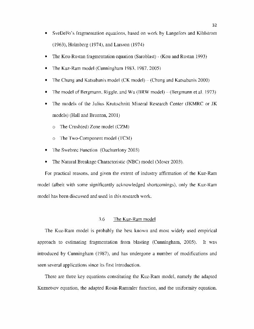
• SveDeFo’s fragmentation equations, based on work by Langefors and Kihlstrom
(1963), Holmberg (1974), and Larsson (1974)
• The Kou-Rustan fragmentation equation (Saroblast) - (Kou and Rustan 1993)
• The Kuz-Ram model (Cunningham 1983, 1987, 2005)
• The Chung and Katsabanis model (CK model) - (Chung and Katsabanis 2000)
• The model of Bergmann, Riggle, and Wu (BRW model) - (Bergmann et al. 1973)
• The models of the Julius Kruttschnitt Mineral Research Center (JKMRC or JK
models) (Hall and Brunton, 2001)
o The Crush(ed) Zone model (CZM)
o The Two-Component model (TCM)
• The Swebrec Function (Ouchterlony 2003)
• The Natural Breakage Characteristic (NBC) model (Moser 2003).
For practical reasons, and given the extent of industry affirmation of the Kuz-Ram
model (albeit with some significantly acknowledged shortcomings), only the Kuz-Ram
model has been discussed and used in this research work.
3.6 The Kuz-Ram model
The Kuz-Ram model is probably the best known and most widely used empirical
approach to estimating fragmentation from blasting (Cunningham, 2005). It was
introduced by Cunningham (1987), and has undergone a number of modifications and
seen several applications since its first introduction.
There are three key equations constituting the Kuz-Ram model, namely the adapted
Kuznetsov equation, the adapted Rosin-Rammler function, and the uniformity equation.
32

33
The Kuznetsov equation predicts the mean particle size resulting from a given blasting
situation as a function of the in situ rock condition and the explosive energy infused into
the blast. The Rosin-Rammler function describes the particle size distribution over the
entire range of fragmentation to be achieved. The uniformity equation predicts the spread
of the distribution around the Rosin-Rammler profile, and is an indicator of the precision
or statistical spread of particle sizes around the expected distribution profile.
Hustrulid (1999) has provided an account of the relationship developed by Kuznetsov
(1973) between the mean fragment size and the blast energy applied per unit volume of
rock (powder factor), expressed as a function of rock type. The development below is
sourced from Hustrulid (1999). According to Kuznetsov,
X is the mean fragment size, cm
A is the rock factor. Rock factor is 7 for medium rocks; 10 for hard, highly
fissured rocks; 13 for hard, weakly fissured rocks
Vo is the rock volume (cubic meters) broken per blast hole.
Vo = Burden * Spacing * Bench Height
Qt is the mass (kg) of TNT containing the energy equivalent of the explosive
charge in each blast hole
3.6.1 The Kuznetsov equation
(3.6)
Where:

Expressing the TNT strength in Equation 3.6 in terms of ANFO strength (where the
relative weight strength of TNT compared to ANFO is 115, ANFO relative strength being
100), then:
34
x = a ( Q ) ° >
Where:
Qe is the mass of explosive being used (kg)
Sanfo is the weight strength of the explosive relative to ANFO
But:
Vo _ 1 Qe K
Where:
3K is the powder factor (or specific charge, in kg/m )
Hence, Equation 3.7 becomes:
(3.7)
(3.8)
X _ A (K )-a8Q1/6 ( ^ y 9730 (3.9)e VSANFO/
The mean fragment size can, therefore, now be calculated from a given powder
factor.

This form (Equation 3.9), as well as that in Equation 3.7, is the preferred form
employed by Cunningham in the Kuz-Ram model.
Various applications have been found for this equation, including the calculation of
the quantity of a given explosive required to achieve a certain mean fragmentation from a
blast.
3.6.1.1 The rock factor, A
Cunningham (1983) reckoned initially that values of rock factor, A, range from 8 to
12, with 8 being the lower limit even for very weak rocks and 12 the upper limit even for
hard rocks. Cunningham has since taken several steps to improve estimates of the factor,
A. A significant milestone along this path was the adoption and modification of Lilly’s
Blastability Index (Lilly 1986; Widzyk-Capehart and Lilly 2001).
Lilly (1986) defined the Blastability Index (BI) as:
BI = 2 [RMD + JPS + JPO + SGI + H] (3.10)
Where:
RMD is the rock mass description
JPS is the joint plane spacing
JPO is the joint plane orientation
SGI is the specific gravity influence
H is rock hardness
Values that Lilly provided for the terms in this relationship are given in Table 3.2.
35

Cunningham (1987) initially proposed an adaptation for Lilly’s scheme as follows:
A = 0.06 x (RMD + JF + RDI + HF) (3.11)
Where:
JF, the Joint Factor, replaces the Joint Plane Spacing (JPS) and Joint Plane
Orientation (JPO) in Lilly’s formulation.
As will be shown in Equation 3.17, this replacement would be subsequently modified
further in Cunningham’s revision of the algorithm.
36
3.6.2 Adoption of the Rosin-Rammler equation
Cunningham observed that the Rosin Rammler formula (see Equation 3.2) provides a
reasonable description of the fragment size distribution in blasted rock, the preferred
formulation being:
- ( - TR = e (3.12)
or
- ( - )nWr = 100e (xcJ (3.13)
Where:
R is the proportion of material retained on a given mesh, x
Wr is the percentage of the weight retained on that mesh
x is a given screen size

xc is the characteristic size, a scale factor dictating the size through which 63.2%
of the particles pass
Cunningham (1983) and Hustrulid (1999) show that xc can be obtained from a
rearrangement of Equation 3.12, such that:
37
llnRj(3.14)
xx nc
Given that the Kuznetsov formula gives the 50%-passing screen size X, then
substituting X for x and R = 0.5 in Equation 2.12, then:
*<= = i d b * (3-15>
The requirement for completeness of the prediction model, then, is to determine “n"
the uniformity constant.
3.6.3 The U niformity equation
From field results, Cunningham (1987) found that, for a square drilling pattern,
1 , S(2-2 - 1 4 D )1? 0 - W)(H)
0.5(3.16)
Where:
n
B is the burden (m)

S is the spacing (m)
D is the hole diameter (mm)
W is the standard deviation of drilling accuracy (m)
L is the total charge length (m)
H is the bench height (m)
For a staggered pattern, ‘n’ increases by 10%.
In general, it is desirable to have uniform fragmentation, so high values of ‘n ’ may be
preferred. Cunningham (1987) has observed the following pattern:
• The normal range of ‘n ’ for blasting fragmentation in reasonably competent
ground is from 0.75 to 1.5, with the average being around 1.0. More competent
rocks have higher values.
• Values of ‘n ’ below 0.75 represent a situation of “dust and boulders” which, if it
occurs on a wide scale in practice, indicates that the rock conditions are not
conducive to control of fragmentation through changes in blasting. Cunningham
observed that “dust and boulders” typically happens when stripping overburden in
weathered ground.
• For values below 1, variations in the uniformity index, ‘n’, are more critical to
oversize and fines. For n = 1.5 and higher, muck pile texture does not change
much, and errors in judgment are less punitive.
• The rock at a given site will tend to break into a particular shape. These shapes
may be loosely termed “cubes”, “plates”, or “shards”. The shape factor has an
important influence on the results of sieving tests, as the mesh used is generally
38

square, and will retain the majority of fragments having any dimension greater
than the mesh size.
3.7 Important limitations to the original Kuz-Ram model
As the mining industry embraced the original Kuz-Ram model, a number of
shortcomings became apparent, as shown below. Some of these shortcomings still exist
today.
i. The model failed to consider the effect of timing on fragmentation (Ouchterlony
2005; Kanchibotla et al. 1999)
ii. It did not expressly consider the effect of gas pressure and brisance
iii. It did not account for microfractures resulting in the broken rock
iv. It did not model fines sufficiently effectively (Ouchterlony 2005)
v. It did not account for boosters and primers
In the light of some the above limitations, Cunningham (2005) proposed a set of
changes to the original Kuz-Ram model. The changes aimed at improving estimation of
mean fragmentation X, and uniformity, ‘n’, both of which he reckoned were partly
outcomes of the initiation methods. He ascribes the possibility of these changes to
advancements related to the introduction of electronic delay detonators.
3.7.1 Important changes to the algorithm
One significant change in the mean fragmentation algorithm lies in the inclusion of a
correction factor, C(A). Need for this correction typically arises when it is apparent that
the rock factor, A, is either greater or smaller than the original algorithm dictates.
39

Cunningham (2005) recommends that, rather than tweak the input, thus possibly losing
some valid input, a correction factor is applied to the rock factor, to adjust to what is
reckoned to be the reasonable value.
There is also a minor change in the sub-algorithm to quantify the Joint Plane Angle
(JPA) influence. This change is as shown in Table 3.3.
The revised algorithm, which has been used in this dissertation, is:
A = 0.06(RMD + RDI + HF)C(A ) (3.17)
40
C(A) has values well within the range 0.5 to 2.

41
Adapted from Latham et al. (2006)
FIGURE 3.1 A schematic of key design features in a bench blast

42
Adapted from Ouchterlony (2003)
FIGURE 3.2 An example of a fragmentation curve

TABLE 3.1 A list of energy factors recommended for various blasting situations
43
Operating SituationRecommended Energy Factor
(kcal/st)
Very weak rock 100
Well jointed, harder rock 140
Average rock 180
Hard rock 220
Blocky, very hard rock 250
Mine-to-mill blasting 350
Very high energy blasts 500
Upper limit 1200
Source: J. Floyd, 2012: Efficient Blasting Techniques

TABLE 3.2: Ratings for Lilly’s rock factor parameters
44
Parameter Description Rating
Rock Mass Description (RMD)
Powdery/Friable 10
Blocky 20
Totally Massive 50
Joint Plane Spacing (JPS)
Close (< 0.1m) 10
Intermediate (0.1 to 1m) 20
Wide (> 1m) 50
Joint Plane Orientation (JPO)
Horizontal 10
Dip out of face 20
Strike normal to face 30
Dip into face 40
Specific Gravity Influence (SGI)
SGI = 25* SG - 50 (where SG is in t/m3)
Hardness (H) Mohr’s Hardness 1 to 10
Adapted from Lilly, 1986

45
TABLE 3.3: Modifications to assigned values for joint plane angle (JPA)
Direction of rock fabric Value 1987 Value 2005
Dip out of face 20 40
Strike out of face 30 30
Dip into face 40 20

CHAPTER 4
PRINCIPLES, TRENDS, AND METHODS FOR COMMINUTION MODELING
AND THE SIMULATION OF CRUSHING SYSTEMS
4.1 Overview
In this chapter, the principles and theories behind the range of process simulation
models used in this research are reviewed. Because comminution processes are typically
supported and accompanied by classification phenomena and processes, the applicable
models for these accompanying phenomena and processes have been included in this
discussion.
4.2 The discussion and reporting of grinding simulation
The original plan for reporting on the outcomes of this research included providing a
detailed discussion of the theory of grinding simulation. The plan also included
providing a complete account of the grinding work that was carried out as part of this
research in anticipation of the need to appraise (by simulation) the grinding performance
of various streams of hypothetical mill feed that may arise from crushing simulated
fragment size distributions for the range of blast designs considered.
In the pursuit of the original research plans, the key findings and conclusions that are
presented in Chapters 7, 8, and 9 demonstrated that the initially anticipated analysis of

grinding are not justified as a central component of this dissertation. However, in view of
the amount of effort devoted to this process, the grinding simulation literature review, the
details of the modeling parameter development, and the grinding simulation work itself
are included as Appendix A. The outcomes presented in this appendix remain valid
considerations for a grinding optimization effort at the mine, for as long as the ores being
treated in the ball mills remain the same as those that were being treated at the time of the
grinding sample collection. Should those ores change, which they will as mining
progresses downwards in the pits, fresh samples of crusher product will need to be taken,
and the full range of grinding tests performed on the material.
In light of the situation described above, the discussions and reviews in this chapter
have been provided with very broad attention to comminution in general, and a very
specific focus on crushing. Minimal space is given to grinding considerations in the main
text.
4.3 The simulation of mineral processing circuits
According to Thomas et al. (2014), “Simulation is the imitation of the operation of a
real-world process or system over time. The act of simulating something first requires
that a model be developed; this model represents the key characteristics or
behaviors/functions of the selected physical or abstract system or process” .
In mineral processing technology, Lynch and Morrison (1999) maintain that,
modeling and simulation are concerned with the design and optimization of circuits.
According to them, realistic simulation relies heavily on the availability of accurate and
47

48
physically meaningful mathematical models, of which there are three types: theoretical,
empirical, and phenomenological.
Detailed discussions about the characteristics and formulation of these models are
well dispersed in literature (Mular 1989; Sastry and Lofftus 1989; Sastry 1990; Wills
2006) and will, therefore, not be given further treatment here.
Bond’s (1952) model is one of three popular empirical energy-size relationships for
the modeling and scale up and simulation of comminution systems. The others are by
Rittinger (1867) and Kick (1883). According to Bond, the energy required for
comminution is proportional to the new crack tip length produced. Reconciling
Rittinger’s and Kick’s laws, a practical form of Bond’s law contains three parameters: a
feed size parameter, a product size parameter, and a work index, all of which are used to
compute the specific energy requirement for a commercial size reduction process. It is
given as:
4.3.1 The Bond model
(4.1)
Where:
E is the Specific Energy, (—t—)kWh
Wi is the Bond’s Work Index
P80 is the 80% product passing size

F80 is the 80% feed passing size
A major problem with Bond’s formulation is that it is inherently a gross over
simplification of especially the grinding system (Herbst and Fuerstenau 1968) and is
typically in error by large margins, increasing design risk by up to ±20 % (Blasket 1970;
Herbst et al. 1977; Smith 1979).
The shortcomings in the performance of the Bond model, especially in wet
comminution systems, seem to arise from its failure to explicitly account for some
important circuit subprocesses in the grinding process (Siddique 1977). Instead, it lumps
them all into a single empirical correlation (Herbst and Fuerstenau 1968; Herbst et al.
1983). These important subprocesses include the breakage kinetics, particle transport
through the mill, and size classification.
Perhaps the most significant detailed phenomenological models for grinding are
derived from population balance considerations (Siddique 1977). These models
explicitly account for the grinding circuit subprocesses, namely, size reduction kinetics,
size classification, and material transport in the mill. By including these critical
elements, the population balance models become significantly more effective than the
simpler energy— size reduction equations.
4.3.2 Justification for the use of modeling and simulation in this research
It is notoriously challenging to include or provide adequately for research work
within the normal mining and processing activity of an operation. Even where an
operation approves such a project, the demands and pressures of production usually and
quickly cause many aspects of such research work to be de-prioritized, and focus tends to
49

be drawn to them only if the production is facing significant enough technical challenges
whose solution may lie in the research outcomes.
Modeling and simulation are essentially nonobtrusive methods and provide a
convenient answer not only for operating mines, but also especially for academic
research. In academic research, the objectives and focus may have little overlap with
those of a particular mine. By using these techniques, it is usually feasible and
convenient to study the processes without necessarily incurring the penalty of the
physical outcome of the processes themselves (Tucker 2001). Thus, modeling and
simulation methods have been used in this work, to investigate all stages from blasting to
grinding.
4.4 The modeling and simulation of crushing systems
A variety of models are available in literature for the simulation and modeling of
crusher performance (King 2012; Wills 2006). Not all of these models take into
consideration the particle size distribution of the feed. To be applicable to this study,
only models which are susceptible to effective simulation of input and output particle size
distributions are considered. In addition, the particle size distribution of the product from
such models would normally be strongly related (directly or indirectly) to the particle size
distribution of the feed. Lastly, the product characteristics arising from such a model
must also bear evidence of the influences of the comminution system and the prevailing
breakage and classification phenomena.
50

4.4.1 The jaw crusher model
The jaw crusher model used in this research is the Empirical Model for Jaw and
Gyratory Crushers (EMJC)). This model is a simple normalized logarithmic distribution
predictor, (Csoke et al. 1996) that is based on the idea that material in the feed smaller
than the gap passes straight through the crusher and the larger material is crushed to a
predefined size distribution that is modeled by the relation:
B(r) = (r/rmax)m
Where:
B is the size distribution function for product arising from feed with size
characteristic “r”, which is defined below
r = dp/GAP
dp is the size of the feed particle being broken
rmax = dp(max)/GAP
dp(max) is the maximum size of the feed particle in the feed stream
GAP is the Open Side Setting (OSS) of the crusher
m is the exponent
In addition to these inputs into the EJMC model, the impact work index
material in this crusher is an important input.
4.4.2 The cone crusher model
The cone crusher model selected for use in this research is the Classification-
Breakage Cycle Model (or CBCM) (after Whiten 1973). This model provides perhaps
51
(4.2)
of the

the most effective and useful description of the crushing action of a crusher. Also
considered the standard model for crushers (Whiten et al. 1973), the CBCM is developed
from population balance considerations, and is amenable to use for jaw, gyratory, and
cone crushers. In this work, the CBCM has been used to simulate the performance of
only the cone crushers.
The model formulation is based on the fact that the operation of a crusher is periodic,
with each period consisting of a nipping action and an opening action. In the opening
stage of the cycle, some fresh feed is taken in, while material already inside and further
up moves downward into the crusher. In the process, some material falls through and
out. This set (or cycle) of events can then be described quantitatively in terms of a
discrete size distribution for both feed and product.
Consider a feed stream with various size classes, i, where i = 1 to n, with class 1
containing the largest particles.
Let:
pi be the fraction of the product in size class i
piF the fraction of feed in size class i
M the mass of material held in the crusher
bij the fraction of particles breaking in size class j that end up in size class i
mi the fraction of material in the crusher in size class i
ci = c(di), the fraction of material in size class i that is retained for breakage
during the next nip of the crusher
W is the mass of total feed that is accepted during a single opening of the crusher,
which is also the mass of product discharged from the crusher.
52

53
In this scheme, the size distribution in a product is completely determined from the
size distribution in the feed and a knowledge of the classification and breakage functions,
ci and bij, respectively. The size distribution in the product can be calculated from the
following relationship:
An account of the development of this relationship is provided by King (2012).
For a specific crusher, this model reduces to the specification of the appropriate
classification and breakage functions. These two features are directly related to the
characteristics of the crusher, rather than to the characteristics of the material.
4.4.2.1 The crusher classification function
For the range d1< dpi < d2, a useful form of the crusher classification function, ci, in
Equation 4.3 is typically of the form:
(4.4)
For dpi <di, ci = 0
For, dpi > d2 . ci = 1
Where:

54
d1 is the smallest size particle that can be retained in the crushing zone during the
opening phase of the cycle
d2 is the largest particle size that can fall through the crushing zone during the
opening phase of the cycle
The parameters, d1 and d2 , are characteristic of the crusher, and are determined
primarily by the setting of the crusher. King (2012) reports that data from crushing
machines indicate that both of these parameters are proportional to the closed side setting
(CSS) of the crusher. For both the standard and short-head Symons cone crushers, the
relationship is as follows:
In general, ai varies from about 0.5 to 0.95, and a2 varies from about 1.7 to 3.5. The
power, n, is usually approximately 2, but can be as low as 1 and as high as 3. The value
of d* is normally set to 0.
4.4.2.2 The crusher breakage function
According to King (2012), the breakage function that describes crushed product
behavior is of the form:
di = ai CSS (4.5)
d2 = a2 CSS + d (4.6)
(4.7)

55
The values of bij are obtained from the cumulative breakage function by the
relationship:
bij = B(Di-1; dpj) - B(Di; d j (4.8)
Where:
bij is the fraction of material that enters size interval i from size interval j.
The values of bjj are determined from the relationship:
bjj = 1-B(Dj; dpj) (4.9)
Where:
bjj is the fraction of material that remains in size interval j after breakage.
4.4.3 Estimation of crusher classification and breakage functions
The parameters in the classification and breakage functions are specific to crusher
type and size. According to King (2012), not many studies have been done to establish
their values under a range of actual operating conditions using predictive equations. The
recommended practical means to estimate these quantities is from measured particle size
distributions in the products from operating crushers. However, once established for a
particular material in a particular crusher, they remain independent of the CSS. Hence,
crusher performance can be simulated as the CSS is varied. This method to estimate
selection and breakage functions has been used in this research.

56
4.4.4 Estimating the crusher work index
Utley (2002) and Luz and Milhomem (2013) maintain that the classical Bond
equation is useful for the estimation of comminution power estimation, including
crushing power. However, this procedure has come under criticism from authors such as
Magdalinovic (1989, 1990) and Magdalinovic et al. (2011), who proposed a modification
(see Jankovic et al., 2004; Luz and Milhomem 2013):
A is a material- and crusher-dependent parameter.
In the absence of a first-principles approach to the determination of the crusher work
index or Magdalinovic’s parameter, A, a representative value for the work index can be
estimated by more practical ways. Of note is the usefulness of a back-calculation method
involving the use of the Operating Work Index (Rajamani 2012; Rowland and McIvor
2009). Based in principle on Bond’s original theory (Section 4.3.1), this approach does
not involve using conventional testing equipment, but instead relies on actual specific
energies expended at the comminution plant (in this case, the crusher) during normal
operation. It also relies on measures from actual (or estimated) feed and product 80%-
passing particle sizes (P80 and F80). The adapted Bond relationship applied at each
crusher in the circuit is as follows (Rajamani 2012; Rowland and McIvor 2009):
(4.10)
Where:

57
E = F = 10WbFf(4.11)
Where:
kWh.E is the specific energy, (—t—)
PC is crusher power, (kW)
Ff is fresh feed rate into crusher (tonnes per hour)
WB is the Bond’s crusher work index (kWh/ton)
P80 is the 80% product passing size, (microns)
F80 is the 80% feed passing size, (microns)
All terms in this relationship, with the exception of the work index, can be obtained
from actual operational data. Hence, the operating work index can be estimated.
It is noteworthy that the value WB, which is also Bond’s crusher work index in
so that:
B(4.12)
Importantly, this relationship makes the value of WB both crusher- and material-
dependent, rather than just material-dependent. Indeed, this phenomenon is observed in
parameter development in Section 6.2.3.

CHAPTER 5
FRAGMENTATION MODELING PARAMETERS, BLAST DESIGNS, AND
FRAGMENTATION PREDICTION
5.1 Overview
In this chapter, three aspects of this research work are treated. Firstly, the rock
characterization procedure used to generate parameters for blast fragmentation modeling
and simulation is presented. This stage of work was almost entirely geotechnical in
content. The outcome was a set of Kuz-Ram factors for the entire suite of rocks treated
in the research.
The second stage involved the development of blast designs. All blast designs
resulting from that phase of work are presented.
The third stage involved prediction of the blast fragment size distributions.
5.2 Determination of rock factor, A
Cunningham’s formula for rock factor is given in equation 3.17 as:
A = 0.06- (RMD + RDI + H F) C(A) (5.1)
Where:
RMD is the Rock Mass Description
RDI is the Rock Density Influence
HF is the Hardness Factor
C(A) is the Correction Factor
In this scheme, the value of RMD is 10 for powdery/friable rock and 50 for massive
rock; and RMD is equal to JF, for vertically jointed rock. These values are fixed and
there is no gradation between them.
The RMD is an in situ rock parameter, and the RDI and HF are laboratory-assessed.
The in situ rock characteristics (RDI) were evaluated with the input of the mine
geologists at W.U.S. Copper. To aid an unbiased and objective characterization of the in
situ rock condition, a questionnaire was developed, based on Cunningham’s algorithm.
By carefully posing questions related to the rock condition and obtaining answers from
the geologists, it was possible to use this questionnaire to evaluate the rock mass
description (RMD). Table 5.1 shows a typical form, populated with answers (from both
in situ and laboratory-derived data), related to the skarn ore in Bom pit. The forms for
the rest of the rock types are presented in Appendix C.
5.2.1 Sample collection and preparation
Specimens of rock of various sizes were obtained from selected piles of blasted ore
and waste at the mine site of W.U.S. Copper. This selection was guided by W.U.S.
Copper personnel, based on the specimens’ apparent representativeness of the visually
assessed physical characteristics of the rock category of interest. Specimens were
59

obtained from both Bom and Sembehun pits, in dimensions ranging in diameter from a
few centimeters (for point load tests) to about a quarter of a meter for coring and use in
uniaxial compressive strength and related tests.
All tests were carried out in the geotechnical laboratories of the Department of
Mining Engineering at the University of Utah.
Preparation of the rock specimens intended for compressive strength testing involved
the casting of the blocks of rock in concrete, to facilitate good positioning and a firm grip
during coring. Four separate blocks of rock (2 ore, 2 waste) were cast in concrete. After
curing, these blocks were cored into cylindrical specimens of two main diameters, using
the radial drill. Cored specimens were cut to sizes suitable for UCS testing, as specified
in ASTM D7012. A total of 17 cores of size NX (nominal 54.7 mm, or 2.16 in.) and six
of 31.4 mm nominal size were obtained. Appendix D shows, in addition to other data,
details of the dimensions of the specimen cores used in this work. The target
Length/Diameter (L/D) ratio was 2:1. However, where it was not possible to achieve that
ratio, the specimen was cut to the nearest ratio possible. Appendix E shows selected
photos of some of the cores produced.
The cut ends of the cylindrical rock cores were ground to achieve smooth and parallel
ends to each specimen. The cores of softer rock (particularly from Bom pit) were not
subjected to grinding, as it was perceived that this would massively degrade the
specimens.
Those specimens whose ends were not ground were observed to have markedly
irregular ends. To ensure that they had the end-parallelism necessary for the strength
tests, the ends of these specimens were lined with a quick-set, epoxy-based filler, and
60

molded between cylinders of stainless steel. Strips of cellophane sheet were used to
promote the separation of the samples from the cylinders. Although end-parallelism was
still not fully achieved, the samples were significantly better than before.
5.2.2 Testing
5.2.2.1 Density tests
All samples were weighed using a Sartorius™ scale model 3713. Their lengths and
diameters were determined using digital calipers. The values from these measurements
were recorded and used to calculate the density of the rocks. The densities so obtained
became key inputs into the derivation of the Kuz-Ram factor.
For good comparison of the density values of the rocks, density data were obtained
from the Ore Control Section at W.U.S. Copper (Appendix F). Overall, the densities
reported by the mine compared well with those calculated. Where differences were
apparent, judgment was used to decide which values to use in the determination of the
Kuz-Ram rock factor.
5.2.2.2 Ultrasonic velocity testing
Ultrasonic velocity testing was carried out on the cylindrical samples. In this
procedure, the p- and s-wave velocities of the specimens were obtained by standard
ASTM procedures (ASTM D 2845 - 00). Primarily, the purpose of this was to obtain
values of the dynamic Young’s modulus of these rocks. According to Cunningham,
(2005) uniaxial compressive strength values for soft rocks are meaningless as an input to
the derivation of rock factor, and should be replaced by the dynamic Young’s Modulus in
61

the algorithm (obtained from ultrasonic velocity testing). The data obtained from this
process are presented along with the core dimension data in Appendix D.
5.2.2.3 Uniaxial Compressive Strength (UCS) testing
UCS tests were performed by standard ASTM methods (ASTM 7012). Two types of
testing machine were used, namely, the Rock Mechanics Testing Machine, (RMTS
machine) and a testing machine specifically constructed for low-strength samples (a low-
strength sample testing machine, or LSTM). The softer samples, predominantly obtained
from Bom Pit, were tested using the LSTM. The harder, larger samples, predominantly
waste rock from Sembehun Pit, which had been cored with NX bits, were tested using the
RMTS machine.
The results obtained from the uniaxial compressive strength tests are summarized in
Appendix G.
5.2.2.4 Point Load Index (PLI) tests
Point load index testing was done on the smaller-sized, irregular-shaped specimens
obtained from the mine site. Procedures were based on the ASTM methods (ASTM
D5731). The results obtained are presented in Appendix H. The results were used to
corroborate UCS values. Where cores were unavailable, the point load test values were
used to estimate the UCS values (example, Sembehun low-grade ore).
62

5.2.3 Computation of rock factor, A
From the results of the various tests outlined above, and using the forms in Table 5.1
and Appendix C, the rock factor was estimated for the major rocks that are blasted at the
mine. The summary of these factors, along with values of various relevant rock
parameters used in this research, are shown in Table 5.2.
In addition to Cunningham’s procedure, Lilly (1986) proposed an alternative method
to determine the Kuz-Ram rock factor. According to Lilly’s experience in Australia, the
rock factor can be obtained from the blastability index by the equation:
A = 0.12*(BI) (5.2)
Using this scheme, a parallel estimate of the rock factor, A, was obtained (see Table
5.2). These results show remarkable similarity. However, only the results from
Cunningham’s model were used in blast prediction in this work.
5.3 Blast design
Eleven blast designs were developed using the Blast Dynamics Energy Factor method
(see Section 3.2.3) (Floyd, n.d.). The base case energy design, which is one of the 11
designs, was that arising from the contract blasting pattern agreed between W.U.S.
Copper and the blasting contractor. These contract patterns are approximately replicated
in Table 5.3. The differences among the energy factors as shown in the table are
accounted for by the differences in design formula used by this researcher and the mine.
63

The researcher retains the use of the Energy Factor method because of its perceived
superiority to the Powder Factor method favored by the mine.
The following are the characteristics of the blast design exercise and its scope:
i. The energy levels chosen for this set of designs range from 100 kcal/st to 400
kcal/st. For each of the six rock categories that are mined by W.U.S. Copper, a
blast design has been developed at each of 10 energy levels, based on Equation
3.1.
ii. The explosive of choice in each design is bulk ANFO. While ANFO is effective
and relatively inexpensive explosive, the peculiar specification of the explosive
does not really matter to the investigation concept. The energy factor is the true
driver of the investigation. However, the energy factor does not address the issue
of differences in certain other strength characteristics such as the brisance and
gas-production capacity. The effect of these other characteristics on blasting
outcomes is beyond the scope of this investigation.
iii. Precise timing has been assumed for NONEL initiation.
5.3.1 Details of blast design
Tables 5.4 to 5.8 are summaries of the patterns resulting from the energy factor-
driven blast designs for each of the lithologies under consideration.
64
5.4 Prediction of blast fragmentation
Using the Kuz-Ram model, predictions of particle size distributions were done. The
results of the ore shot size prediction are provided in Table 5.9. Figures 5.1, 5.2, and 5.3

are graphs showing the ore particle size distributions from that prediction. Table 5.10 is
the result of the predictions of waste shot particle size distributions. Figures 5.4 and 5.5
are plots of these particle size distributions.
65

% Pa
ssin
g st
ated
si
ze
Size (cm)
FIGURE 5.1 Plot of fragment size distribution prediction for Bom ore. Fragment size distributions are shown at different blastenergies
99
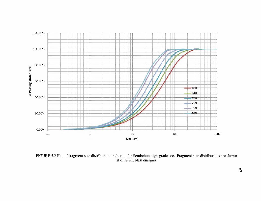
% Pa
ssin
g st
ated
si
ze120.00%
100.00%
80.00%
60.00%
40.00%
20.00%
0.00%0.1
0
140
180
— 250
— 35/in
0n
10
Size (cm)
100 1000
FIGURE 5.2 Plot of fragment size distribution prediction for Sembehun high-grade ore. Fragment size distributions are shownat different blast energies
1
67

% Pa
ssin
g st
ated
si
ze
FIGURE 5.3 Plot of fragment size distribution prediction for Sembehun low-grade ore. Fragment size distributions are shown atdifferent blast energies
89

% Pa
ssin
g st
ated
si
ze
FIGURE 5.4 Plot of fragment size distribution prediction for waste rock (limestone). Fragment size distributions are shown atdifferent blast energies
69

% Pa
ssin
g st
ated
si
ze120.00%
100.00%
80.00%
60.00%
40.00%
20.00%
0.00%
/0
/ / ?j r j r
/ / / JJ r > I /
/ f / j rI f / f f
/ / / / / fy / V y /
/ / / / // A r
f / / / /1CH 7̂I f > / > * J f Base Case (164.7)
y y / / / / 100« / >y , f
J r / / 1 140
Jf / / 180AVA\ r
J f 4?A / / / 250.
yr
/ rA f\ 350Va
u \ 1 400
---------- — — — — —— - - ----------— — — — - - — — — ——
—^ — — —
___+---------- 1— — — — —— — ----------— — — - ------ — — — ——
0.1 10
Size (cm)
100 1000
FIGURE 5.5 Plot of fragment size distribution prediction for granodiorite. Fragment size distributions are shown at different blastenergies
1
70

71
TABLE 5.1 A sample of the form used to compute the Kuz-Ram rock factor, A.
Estimation of the Kuz-Ram Rock Factor, A
A = 0.06 * (RMD + RDI + HF) * C(A)A = Kuz-Ram Factor RDI = Rock Density Influence FactorRMD = Rock Mass Description________________ HF = Hardness Factor C(A) = Correction Factor
Rock Tvne: Bom Ore (Soft)
Section 1: RMDRMD = 10 for powdery/friable rock; RMD = 50 for massiver Rock; RMD = JF, for vertically jointed
Section 1a: Rock Mass Description (RMD)Please choose yes (Y) to only one of the following three questions:
i. Is this rock friable (powdery)?(y/n) nii. Is this rock massive, with no jointing, or with jo int spacing > blast hole spacing ? (y/n)iii. Is the rock vertically jointed? (y/n) y
n
Section 1b: Joint Factor, JF - (Only valid if you answered "Y" to Question iii in Section 1a, above)Note: JF = (JCF * JPS) + JPA JF = Joint Factor JCF = Joint Condition Factor JPA = Vertical Joint Plane Angle Factor JPS = Joint Plane Spacing FactorJCF Range of values: 1 to 2Describe th joint condition in the box below. Please, choose only one of three options, namely: "Tight", "Relaxed" or "Gouge-filled": if "Tight", input "1"; if "Relaxed", input "1.5";If joint is "gouge-filled", input "2"W hat is the condition of the joint? (1, 1.5 or 2) 1.5JPS Range: 10 to 50Relevant factors: Reduced Pattern (P) and Joint Spacing (S) P = Reduced Pattern = (B*S)05What is the average spacing of joints, in meters? 0.25 p = 4.56What is the blast Burden (in meters)? 4.27 95% P 4.33What is the blast Spacing (in meters)? 4.88 JPS 20.00JPA Note that only one answer can be "Yes", although all can be "No"Do the joints dip out of the face at >30o? (Y or N) yDo the joints dip into the face at >30o? (Y or N) n JPA 40Do the joints Strike out of the face? (Y or N) n RMD 65Section 2: RDI (Rock Density Influence)Rock Density (kg//m3) 3268Rock Density Influence Factor (RDI) = 31.7
Section 3: Hardness Factor (HF)Young's Modulus, Y (Gpa)UCS (MPa)
44.5628.76
Hence, Hardness Factor, HF = 14.85
Kuz-Ram Factor |Uncorrected Kuz-Ram Factor 6.69Correction 1Kuz-Ram Factor (Estimate) 6.69

TABLE 5.2 Summary of the estimated rock characteristics
Rock SG (t/m3) K-Factor 1 K-Factor2 (Lilly) Blastability Index P-wave vel (km/s)Bom ore (Skarn) 3 . 2 7 6 . 6 9 6 . 9 4 5 7 . 8 5 4 . 4 3
Sembehun high-grade (soft) (Skarn) 2 . 9 7 6 . 5 1 5 . 4 3 5 4 . 3 3 5 . 3 6
Sembehun low-grade (hard) (Skarn) 2 . 7 2 8 . 4 9 8 . 0 4 5 7 . 0 4 5 . 3 6
Waste (Limestone) 2 . 5 9 8 . 3 3 7 . 9 4 5 6 . 1 9 5 . 9 2
Monzonite 2 . 6 6 8 . 7 2 8 . 0 7 5 7 . 2 4 5 . 9 2
Granodiorite 2 . 5 6 8 . 1 9 6 . 0 9 5 0 . 7 9 5 . 9 2
ZL

TABLE 5.3 The contract blast pattern and its approximate representation in this research work. (Note: 1 ft = 0.3048 m)
Rock
Contract Pattern Research Approximation
Burden (ft) Spacing (ft)Powderfactor
(lb/yd3)Burden (ft) Spacing (ft)
Powderfactor
(lb/yd3)
Energyfactor
(kcal/st)Bom 14 16 0 . 6 1 4 . 0 16 . 1 0 . 9 12 9 . 0
Sembehun high- grade
14 16 0 . 6 1 4 . 0 16 . 1 0 . 9 1 4 2 . 0
Sembehun low- grade
14 16 0 . 6 1 4 . 0 16 . 1 0 . 9 1 5 5 . 0
W aste 14 16 1 . 2 1 4 . 0 16 . 1 0 . 9 1 6 2 . 5
M onzonite 12 14 1 . 3 5 12 . 2 1 4 . 0 1 . 2 2 1 0 . 2
Granodiorite 14 16 1 . 2 1 4 . 0 16 . 1 0 . 9 16 4 . 5
73

TABLE 5.4 Blast pattern for Bom ore (Note: 1 ft = 0.3048 m)
E xplosive energy (kcal/st) 129 100 140 160 180 220 250 280 300 350 400
Bench height, L (ft) 20 20 20 20 20 20 20 20 20 20 20
Burden (ft) 1401 15.92 13.45 12.58 1186 10.73 10.07 9 .51 9 .19 8 .51 7 .96
Spacing (ft) 1612 18.30 15.47 14.47 1364 12.34 11.58 10.94 10.57 9 .78 5 15
Subdrill (ft) 394 3 .94 394 3.94 394 3 .94 3 .94 3.94 3 .94 3 .94 3 .94
Stemming (ft) 1238 1238 1238 1238 1238 12 38 1238 1238 1238 1238 1238
T otal hole length (ft) 2394 23.94 23.94 23.94 2394 23.94 23.94 23.94 23.94 23.94 23.94
L/B (Stiffness ratio) 143 1 .26 1.49 1 .59 169 1 .86 1 .99 2 .10 5 18 2 .35 5 51
P owder factor (lb/st) 032 0 .25 035 0.40 5 .45 0 .54 0 .62 0.69 0 .74 0 .87 0 .99
P owder factor (lb/yd3) 5 88 0 .68 095 1 .09 523 1 .50 1.70 1 .91 2.04 2 .39 2 .73
74

TABLE 5.5 Blast pattern for Sembehun high-grade ore (Note: 1 ft = 0.3048 m)
Explosive energy (kcal/st) 142 100 140 160 180 220 250 280 300 350 400Bench height (L) (ft) 20 20 20 20 20 20 20 20 20 20 20Burden (ft) 1402 16.71 14.12 1321 12.45 11.26 10.57 1 98 9.65 8.93 835Spacing (ft) 1612 1921 1624 15.19 1432 12.95 12.15 11.48 11.09 10.27 9.61Subdrill (ft) 394 1 94 3.94 1 94 1 94 1 94 1 94 1 94 1 94 3.94 1 94Stemming (ft) 1238 1238 1238 1238 1238 1238 1238 1238 1238 1238 1238Total hole length (ft) 2394 23.94 23.94 23.94 2394 2394 2394 2394 2394 23.94 2394L/B (Stiffness ratio) 1.43 120 1.42 1.51 161 1.78 1.89 2.00 1 07 2.24 239Powder factor (lb/st) 035 0.25 1 35 1 .40 0.45 0.54 1 62 1 69 1 .74 0.87 1 99Powder factor (lb/yd3) 088 062 0.87 1 99 111 136 155 1.73 1.86 2.17 1 .47
75

TABLE 5.6 Blast pattern for Sembehun low-grade ore (Note: 1 ft = 0.3048 m)
Explosive Energy (kcal/st) 155 100 140 160 180 220 250 280 300 350 400
Bench Height, L (ft) 20 20 20 20 20 20 20 20 20 20 20
Burden (ft) 14.00 17.44 14.74 13.78 13.00 11.75 11.03 10.42 10.07 9.32 8.72
Spacing (ft) 16.10 20.05 16.95 15.85 14.94 13.52 12.68 11.98 11.58 10.72 10.03
Subdrill (ft) 3.94 3.94 3.94 3.94 3.94 3.94 3.94 3.94 3.94 3.94 3.94
Stemming (ft) 12.38 12.38 12.38 12.38 12.38 12.38 12.38 12.38 12.38 12.38 12.38
Total Hole length (ft) 23.94 23.94 23.94 23.94 23.94 23.94 23.94 23.94 23.94 23.94 23.94
L/B (Stiffness ratio) 1.43 1.15 1.36 1.45 1.54 1.70 1.81 1.92 1.99 2.15 2.29
Powder Factor (lb/st) 0.38 0.25 0.35 0.40 0.45 0.54 0.62 0.69 0.74 0.87 0.99Powder Factor (lb/yd3) 0.88 0.57 0.80 0.91 1.02 1.25 1.42 1.59 1.70 1.99 2.27
9 L

TABLE 5.7 Blast pattern for limestone (Note: 1 ft = 0.3048 m)
Explosive energy (k ca l/st) 162.5 100 140 160 180 220 250 280 300 350 400
B e n c h height, L (ft) 20 20 20 20 20 20 20 20 20 20 20
Burden (ft) 14 0 1 17 8 6 1 5 0 9 1412 1 3 3 1 1 2 0 4 111.30 110.67 10 3 1 1 91.55 8 9 3
Sp acing (ft) 1611 1 0 5 4 17 3 6 16.24 1 5 3 1 1 3 8 5 112.99 112.27 111.86 110.98 1110.27
Subdrill (ft) 3 9 4 3 9 4 3 9 4 3 9 4 3 9 4 1 9 4 1 31.94 1 9 4 3 9 4 1 9 4 1 9 4
Stem m ing (ft) 1 2 3 8 1 2 3 8 1 2 3 8 1 2 3 8 1 2 3 8 1 2 3 8 1 2 3 8 1 2 3 8 1 2 3 8 1 2 3 8 1 2 3 8
T o ta l hole length (ft) 1 3 9 4 2 3 9 4 1 3 9 4 1 3 9 4 2 3 9 4 2 3 9 4 1 123.94 2 3 9 4 2 3 9 4 2 3 9 4 2 3 9 4
L/B (S tiffn ess ratio) 1.43 112 132 1.42 150 11.66 1 11.77 1 11.87 1 11.94 21.09 21.24
P ow d er fa c to r (lb/st) 0.40 0 2 5 0 3 5 0.40 0 .45 1 01.54 1 01.62 10.69 10.74 10.87 01.99
P owder fa c to r (lb/yd3) 0 8 8 0 5 4 0.76 0 8 7 0 9 7 1 11.19 1 35 111.52 111.62 11.89 1 21.17
77

TABLE 5.8 Blast pattern for granodiorite (Note: 1 ft = 0.3048 m)
Explosive energy (kcal/st) 164 7 100 140 160 180 2 20 2 50 28 0 3 0 0 3 5 0 40 0
Bench height, L (ft) 20 20 20 20 20 20 20 20 20 20 20
Burden (ft) 14 0 0 117 9 7 115 19 14 2 1 13 .40 12 12 1 111 37 10 7 4 10 3 8 19 61 8 9 9
Spacing (ft) 16 10 20 6 7 117 47 16 3 4 15 .40 1 113 9 3 13 0 7 12 3 5 111 9 3 11.05 1033
Subdrill (ft) 3 9 4 13 9 4 13 9 4 3 9 4 3 9 4 1 13 9 4 13 9 4 13 9 4 13 9 4 13.94 3 9 4
Stemming (ft) 12 3 8 12 3 8 12 3 8 12 3 8 12 3 8 12 3 8 12 3 8 12 3 8 12 3 8 1 238 1238
Total hole length (ft) 13 9 4 23 9 4 23 9 4 13 9 4 23 9 4 13 9 4 23 9 4 13 9 4 23 9 4 13 9 4 23 9 4
L/B (Stiffness ratio) 11 43 11 11 132 141 1 .49 1 11 65 11 76 186 11 9 3 2 0 8 2 2 3
Powder factor (lb/st) 0 .41 0 2 5 0 3 5 0 .40 0 4 5 0 5 4 0 62 0 6 9 0 .74 0 8 7 0 9 9
Powder factor (lb/yd3) 0 8 8 0 5 3 0 7 5 0 8 6 0 9 6 118 11 34 150 1 6 0 187 2 14
78

TABLE 5.9 Particle size distributions predicted for a range of blasting energy factors within the various ore types
E. F a c to r (k c a l/s t) 129 142 155 100 140 160 180 2 20
M a te r ia l -Bum s h g s l g Bum s h g s l g Bum s h g s l g Bum s h g s l g B um s h g s l g Bum s h g s l g
I ic h e s cm
384 .00 975 36 100 00% 100 .00% 100 .00% 100 00% 100 00% 100 00% 100 .00% 100 00% 100 00% 100 00% 100 00% 100 00% 100 00% 100 00% 100 00% 100 00% 100 00% 100 00%
192 .00 487 68 100 00% 100 .00% 100 .00% 99 99% 99 96% 9 3 100 .00% 100 00% 100 00% 100 00% 100 00% 100 00% 100 00% 100 00% 100 00% 100 00% 100 00% 100 00%
96 .00 243 84 99 75% 99 72% 99 42% 98 64% 69 95 19% 99 83% 99 69% 98 94% 99 94% 99 88% 99 53% 99 98% 99 96% 99 80% 100 00% 99 99% 99 97%
48 .00 12192 94 09% 93 82% 89 97% 87 67% 85 51% 236 94 97% 93 56% 87 21% 96 85% 95 78% 90 77% 98 05% 97 26% 93 41% 99 27% 98 87% 96 73%
30 .00 76 20 66 8137% 593 332 2996 58 07% 83 24% 39 8996 87 08% 84 95% 74 73% 90 10% 88 18% 78 90% 6249
CQ29 85 49%
24 .00 60 96 73 57% 73 35%
s46 63 91% 6166% 49 53% 75 31% 2 7 60 53% 79 72% 33 5356 83 41% 8112% 6996 89 01% 87 02% 77 04%
12 .00 30 48 46 53% 664 63
393 37 86% 27 71% 48 02% 46 24% 234 3 52 12% 50 15% 37 59% 55 96% 53 83% 40 78% 8726 356 46 88%
6 .00 15 24 25 52% 25 80% 18 51% 21.47% 21.04% 14 28% 3862 25 57% 17 31% 28 82% 27 85% 18 91% 31.23 30 11% 20 54% 8953 34 51% 23 81%
3 .00 26 12 94% 2213 8 73% 1111% 11.06% 7 05% 13 35% 13 11% 8 24% 14 52% 14 20% 8 90% 15 71% 15 30% 9 60% 18 09% 35 1104%
1 50 3 81 6 31% 6 51% 4 .00% 5 57% 5 65% 3 41% 6 48% 6 47% 3 81% 996 396 4 06% 7 50% 7 41% 334 8 56% 8 40% 4 90%
0 .75 1 90 3 01% 3 14% 180% 2 75% 2 84% 36 3 08% 3 12% 1.74% 3 28% 3 30% 182% 3 49% 3 50% 192% 393 3 90% 2 13%
0 38 0 95 1.43% 150% 0 81% 135% 1.42% 0 78% 1.45% 150% 0 79% 153% 156% 0 81% 1 61% 164% 0 85% 1.78% 180% 0 92%
0 18 0 48 0 68% 0 73% 0 37% 0 67% 0 71% 0 37% 0 69% 0 72% 63 0 72% 0 74% 0 37% 0 75% 0 77% 0 38% 0 81% 0 83% 0 40%
0 .09 0 24 23 0 35% 0 16% 23 63 0 18% 23 0 34% 0 16% 33 0 35% 0 16% 0 34% 63 0 17% 0 37% 0 38% 0 17%
% o / s 18 34% 18 63% 26 41% 27 67% 30 08% 4193% 16 76% 19 07% 30 11% 12 92% 15 05% 25 27% 9 90% 1182% 2110% 5 74% 7 20% 14 51%
O /S in
C l u s h e r f e e d21.1% 33.2% 22.0% 17.7% 14 .3% 9 .1%
U/S in C r u s h e r
F e e d78.9% 66.8% 78.0% 82 .3% 85 .7% 90 .9%
Note: SHG refers to Sembehun high-grade ore; SLG refers to Sembehun low-grade ore.
79

TABLE 5.9 (Continued)
E. Factor (kcal/st) 250 280 300 350 400
Material -Bum SHG SLG Bum SHG SLG Bum SHG SLG Bum SHG SLG Bum SHG SLG
Inches cm
384 975.36 100.00% 100.00% 100.00% 100.00% 100.00% 100.00% 100.00% 100.00% 100.00% 100.00% 100.00% 100.00% 100.00% 100.00% 100.00%
192.00 487.68 100.00% 100.00% 100.00% 100.00% 100.00% 100.00% 100.00% 100.00% 100.00% 100.00% 100.00% 100.00% 100.00% 100.00% 100.00%96.00 243.84 100.00% 100.00% 99.99% 100.00% 100.00% 100.00% 100.00% 100.00% 100.00% 100.00% 100.00% 100.00% 100.00% 100.00% 100.00%
48.00 121.92 99.66% 99.43% 98.11% 99.84% 99.72% 98.93% 99.91% 99.82% 99.27% 99.98% 99.95% 99.73% 99.99% 99.98% 99.90%
30.00 76.20 96.23% 95.08% 89.16% 97.54% 96.66% 91.97% 98.16% 97.43% 93.45% 99.12% 98.68% 96.12% 99.59% 99.33% 97.74%24.00 60.96 91.99% 90.27% 81.49% 94.20% 92.74% 85.17% 95.33% 94.04% 87.24% 97.32% 96.40% 91.33% 98.48% 97.84% 94.18%12.00 30.48 67.43% 65.00% 51.17% 71.49% 69.02% 55.20% 73.93% 71.46% 57.75% 79.23% 76.83% 63.62% 83.53% 81.25% 68.80%
6.00 15.24 39.25% 37.69% 26.25% 42.48% 40.75% 28.67% 44.55% 42.73% 30.26% 49.48% 47.44% 34.17% 54.03% 51.83% 37.95%3.00 7.62 19.87% 19.19% 12.14% 21.63% 20.85% 13.25% 22.79% 21.94% 14.00% 25.66% 24.65% 15.88% 28.46% 27.29% 17.75%
1.50 3.81 9.37% 9.16% 5.35% 10.18% 9.92% 5.81% 10.73% 10.43% 6.12% 12.09% 11.71% 6.90% 13.44% 12.98% 7.69%
0.75 1.90 4.27% 4.22% 2.30% 4.61% 4.55% 2.48% 4.84% 4.76% 2.60% 5.42% 5.31% 2.90% 6.01% 5.87% 3.22%0.38 0.95 1.92% 1.92% 0.98% 2.06% 2.06% 1.05% 2.15% 2.15% 1.09% 2.39% 2.37% 1.21% 2.64% 2.60% 1.33%
0.18 0.48 0.87% 0.88% 0.42% 0.92% 0.94% 0.45% 0.96% 0.97% 0.47% 1.06% 1.06% 0.51% 1.16% 1.16% 0.55%
0.09 0.24 0.39% 0.40% 0.18% 0.41% 0.42% 0.19% 0.42% 0.43% 0.20% 0.46% 0.47% 0.21% 0.50% 0.51% 0.23%
% O/S 3.77% 4.92% 10.84% 2.46% 3.34% 8.03% 1.84% 2.57% 6.55% 0.88% 1.32% 3.88% 0.41% 0.67% 2.26%
O/S in Crusher feed6.5% 4.6% 3.7% 2.0% 1.1%
U/S in C rusher Feed93.5% 95.4% 96.3% 98.0% 98.9%
Note: SHG refers to Sembehun high-grade ore; SLG refers to Sembehun low-grade ore.
08

TABLE 5.10 Particle size distributions predicted for a range of blasting energy factors within limestone (LS) and granodiorite (GD)
E Factor (kcal/st) 162.5 164.7 100 140 160 180 220Material........ LS GD LS GD LS GD LS GD LS GD LS GD
Inches cm
384 975.36 100.00% 100.00% 100.00% 100.00% 100.00% 100.00% 100.00% 100.00% 100.00% 100.00% 100.00% 100.00%
192.00 487.68 100.00% 100.00% 99.76% 99.90% 99.99% 100.00% 100.00% 100.00% 100.00% 100.00% 100.00% 100.00%96.00 243.84 99.45% 99.83% 94.52% 97.40% 98.69% 99.51% 99.39% 99.80% 99.73% 99.92% 99.95% 99.99%
48.00 121.92 90.31% 95.89% 75.22% 85.55% 86.23% 93.29% 89.92% 95.48% 92.69% 96.98% 96.25% 98.66%
30.00 76.20 74.22% 86.33% 57.21% 71.57% 68.85% 81.83% 73.66% 85.56% 77.84% 88.56% 84.51% 92.88%
24.00 60.96 64.91% 79.61% 48.85% 64.13% 59.61% 74.61% 64.35% 78.74% 68.64% 82.23% 75.97% 87.67%
12.00 30.48 37.49% 54.73% 27.54% 41.92% 33.92% 50.11% 37.10% 53.88% 40.20% 57.41% 46.15% 63.75%
6.00 15.24 19.01% 32.63% 14.34% 25.02% 17.26% 29.73% 18.81% 32.08% 20.39% 34.40% 23.57% 38.86%
3.00 7.62 9.02% 17.87% 7.17% 14.15% 8.30% 16.39% 8.94% 17.58% 9.61% 18.80% 11.01% 21.23%1.50 3.81 4.15% 9.34% 3.51% 7.77% 3.88% 8.68% 4.12% 9.21% 4.38% 9.77% 4.94% 10.92%
0.75 1.90 1.88% 4.76% 1.70% 4.19% 1.79% 4.49% 1.87% 4.71% 1.96% 4.94% 2.17% 5.44%
0.38 0.95 0.85% 2.40% 0.82% 2.24% 0.82% 2.30% 0.84% 2.38% 0.87% 2.47% 0.95% 2.68%
0.18 0.48 0.39% 1.22% 0.40% 1.21% 0.38% 1.19% 0.39% 1.21% 0.39% 1.24% 0.42% 1.32%
0.09 0.24 0.17% 0.61% 0.19% 0.64% 0.17% 0.60% 0.17% 0.61% 0.17% 0.62% 0.18% 0.64%
Determination of Oversise in waste blasts
% U/S 97.16% 98.85% 89.69% 94.44% 95.58% 97.96% 97.02% 98.72% 97.97% 99.18% 99.02% 99.66%
% O/S 2.84% 1.15% 10.31% 5.56% 4.42% 2.04% 2.98% 1.28% 2.03% 0.82% 0.98% 0.34%
81

TABLE 5.10 (Continued)
E. Factor (kcal/st) 250 280 300 350 400Material —
LS GD LS GD LS GD LS GD LS GDInches cm
384 975.36 100.00% 100.00% 100.00% 100.00% 100.00% 100.00% 100.00% 100.00% 100.00% 100.00%
192.00 487.68 100.00% 100.00% 100.00% 100.00% 100.00% 100.00% 100.00% 100.00% 100.00% 100.00%
96.00 243.84 99.99% 100.00% 100.00% 100.00% 100.00% 100.00% 100.00% 100.00% 100.00% 100.00%
48.00 121.92 97.78% 99.29% 98.70% 99.62% 99.10% 99.75% 99.65% 99.92% 99.87% 99.97%
30.00 76.20 88.28% 95.03% 91.20% 96.55% 92.76% 97.30% 95.60% 98.55% 97.38% 99.22%
24.00 60.96 80.46% 90.66% 84.19% 92.94% 86.32% 94.15% 90.54% 96.37% 93.54% 97.75%
12.00 30.48 50.35% 67.93% 54.31% 71.66% 56.82% 73.91% 62.61% 78.82% 67.75% 82.84%
6.00 15.24 25.94% 42.05% 28.30% 45.10% 29.85% 47.05% 33.66% 51.65% 37.34% 55.89%
3.00 7.62 12.09% 23.03% 13.17% 24.81% 13.90% 25.98% 15.73% 28.84% 17.56% 31.61%
1.50 3.81 5.37% 11.80% 5.82% 12.68% 6.12% 13.27% 6.89% 14.73% 7.67% 16.18%
0.75 1.90 2.33% 5.83% 2.51% 6.23% 2.62% 6.50% 2.92% 7.17% 3.23% 7.84%
0.38 0.95 1.01% 2.84% 1.07% 3.01% 1.12% 3.13% 1.23% 3.42% 1.35% 3.72%
0.18 0.48 0.44% 1.39% 0.46% 1.46% 0.48% 1.51% 0.52% 1.64% 0.57% 1.77%
0.09 0.24 0.19% 0.67% 0.20% 0.70% 0.20% 0.72% 0.22% 0.77% 0.23% 0.82%
D e te rm in a tio n o f O ve rs ise in w a s te b lasts
% U/S 99.43% 99.82% 99.67% 99.90% 99.77% 99.94% 99.91% 99.98% 99.97% 99.99%
% O/S 0.57% 0.18% 0.33% 0.10% 0.23% 0.06% 0.09% 0.02% 0.03% 0.01%
82

CHAPTER 6
ESTIMATION OF CRUSHER SIMULATION PARAMETERS
6.1 Overview
In this chapter, the procedures that were used to generate the crushing simulation
parameters are described. Due to the limitations discussed in Sections 4.4.3 and 4.4.4, no
direct testing could have been done to generate those parameters. Therefore, indirect
methods of estimation were used.
6.2 Estimation of crushing simulation parameters
The crusher parameters which required estimation for use in this simulation work are
listed in Table 6.1, each parameter in relation to the crusher to which it is relevant.
The parameter that is common to all the crushers is the crusher work index. In
addition, the cone crushers (Cones 1 and 2) require the classification and breakage
functions to be estimated. As discussed in Section 4.3.2.1 (and in King 2012), previous
work has provided viable ranges for these latter parameters, and these ranges were
explored in this work.
In order to be considered valid, the estimated parameters had to meet the following
criteria:

i. The use of the set of estimated parameters must lead to the prediction of a particle
size distribution of simulated final product that is comparable to the particle size
distribution actually measured at the crusher product stockpile.
ii. For baseline operating feed size distributions, the simulated energy consumption
at the crusher must be roughly identical to that observed under baseline operating
conditions.
Obtaining a fair representation of blast product size distribution on-site for validation
purposes was a challenge. Kuz-Ram predictions are averages, and values estimated by
photo-granulometry are often very localized and tend to depart significantly from shot
averages. Consequently, a very rough approximation was made on the basis of degree of
oversize produced by the blasts. The prediction of ore oversize in this work is a mean of
about 21%, and a maximum of 26%. Observed oversize ranged from about 7% to about
20% in ore. The researcher’s judgment is that, given the natural inhomogeneities in
rocks, and the lack of resources to do detailed verification and validation of photo
granulometry with sieving of a whole muckpile, this is an acceptable difference. The
simple and broad assumption is made, therefore, that the crusher feed particle size
distribution produced by the contract blasting practice is roughly equivalent to that which
is predicted by the revised Kuz-Ram model in this research.
6.2.1 Preliminaries for parameter estimation
The following preliminaries were carried out, leading to the parameter estimation
process itself.
84

i. In MODSIM simulation package, the crushing circuit was built (see Figure 6.1),
with features including a jaw crusher, two cone crushers, screens, and feed and
product stockpiles.
ii. Characteristics of the circuit were specified, including crusher gap dimensions,
open and closed side settings, screen perforation sizes, dimensions of all screen
surface areas, screen inclinations, and circuit paths between crushers, screens, and
crushers. Details of the circuit characteristics are provided in Appendix I
(crushing circuit parameters).
iii. The feed characteristics were specified. These characteristics included the ore
type (Bom ore, Sembehun low-grade ore, and Sembehun high-grade ore), density,
and particle size distribution. The base case particle size distribution specified
was a modified form of that predicted by the Kuz-Ram model for the blast pattern
established by the contractor. The modification was done to account for the
contribution of secondary breakage of all oversize (>30 inches) ore. The particle
size distribution of the secondary-broken ore was assumed to be identical to the
size distribution of the blast-generate sub-30-in material. This method of size
reconstitution was used for all the crusher feeds produced by the various energy
factor blasts (Tables 6.2a, b, c).
iv. Key process features were specified. These features included the head feed rates
and the feed blending proportions. Blending was in the ratio:
Bom/Sembehun high-grade/Sembehun low-grade (1:1:1)
v. A preliminary and arbitrary crusher work index value of 30 kWh/t was assumed.
85

6.2.2 Crusher and screen settings and characteristics
An important aspect of the specifications that were made in the simulation of the
crushing system was the set of physical characteristics and settings of the crushers and
screens in the system. To be representative of the operating situation at the mine, the data
(dimensions and settings) of the equipment at the mine were obtained and used as input,
as required, at the model parameter specification stage of the simulation.
The data specified in this research have been presented in Tables 6.3a (settings and
features of the jaw crusher), 6.3b (settings and features of the cone crushers), 6.3c
(settings and features for Screen 1), and 6.3d (settings and features for Screen 2).
6.2.3 The crusher breakage and classification functions
i. These two functions were estimated for only the cone crushers.
ii. Initially, the crusher breakage and classification functions were specified in
MODSIM to match average values of the recommended ranges of setting for both
the breakage and classification functions. These ranges are mentioned in Section
4.4.2.I.
iii. A simulation was then run, and the simulated product particle size distributions
overlain on a plot of the actual mill feed (or crusher run) particle size distribution.
Details of the sampling and size analysis procedure for mill feed are given in
Appendix A. After each run, the departure from the reference plot formed the
basis of adjustment of parameters. All the parameters were gradually adjusted in
suitable directions, until an approximate overlap was achieved (see Figure 6.2).
The settings at which this approximate overlap occurred were chosen as the
86

87
circuit’s parameter settings for the rest of the simulation. These settings are
presented in Table 6.4.
6.2.4 The crusher work index
i. The crusher work index was estimated using the operating work index method
described in Section 4.4.4, using the equation:
All terms are as described in Equation 4.11.
ii. For the reconstituted base case feed (simulated) and crushing product (also
simulated), the 80% passing sizes F80 and P80 were determined. The 80% passing
feed and product sizes for each of the three crushers were determined.
iii. Values of crusher power draw at the time of the crusher product sampling were
obtained from the mine power team.
iv. Setting ( - ^ — ) = k, and using average crusher power draw (Pc) and feed\VP80 VF80/
tonnes of fresh feed rate (Ff), the operating work index Wi(o) was computed as
shown in the table.
v. Assuming motor efficiencies of 80% at each crusher motor, an estimate of true
work index, Wi, was made by de-rating the operating work index (Wi(o)).
However, the operating work index was the value eventually used in all
subsequent simulations, as no provision lies within MODSIM to account for

motor efficiency in the estimation of power draw. A weighted average operating
work index of 20.86 kWh/t is calculated (prorated by mass flow through the
plant), and a “true” work index estimate of 16.69 kwh/t is made. This value is
consistent with various published values of typical copper ores or in related rocks
such as dolomite in skarn deposits (from 1.8 to 40 kWh/t - and averaging 12 to 20
kWh/t) (Bergstrom 1985; Nematollahi 1994; Tavares and Carvalho 2007). All
values of input parameters leading to this estimate, as well as the estimate of the
crusher work index, are shown in Table 6.5.
vi. The variation of crusher work index in the different crushers for the blended ore is
in line with Magdalinovic’s observation (Section 4.4.4) which indicates that the
work index is material and crusher specific.
6.2.5 Verification of crushing simulation parameters
In Table 6.5, note that the power draw for each crusher is the same as that provided
by the power supply staff at W.U.S. Copper. This equality of predicted and actual values
of power draw meets one of the criteria for parameter verification, as specified in i and ii
of Section 6.2. The other validation is provided by the approximate overlap of actual and
simulated product particle size distributions, as shown in Figure 6.2
88

29
Jaw Crusher
Screen
1
200.02 100
155 0
21
18
241.16 100
148 0
241.16 100
10.3 0
114.16 100
4.25 0
Fresh Feed to Jaw Crusher
200.02 100
491 0
1 +
163.66 100
13.5 0
163.66 100
7.02 0
85.86 100
4.43 0
19
200.02 100
4.33 0
} Screen 2
Legend
20
t/h % Sol
P80 (mm) L/m in
Crusher Final Product [Mill Feed;
FIGURE. 6.1 Flowsheet of the crushing circuit, showing mass flow. This mass flow is based on jaw crusher feed size estimates from the blend of fragmentation profiles from contract blasts
89

Cum
ulat
ive
frac
tion
pass
ing
FIGURE. 6.2 Parameter verification plot of simulated and actual product particle size distributions. The test crush simulation product is overlaid on the measured crusher product (mill feed) particle size
profile. 06

91
TABLE 6.1 The set of parameters whose estimation was required for the simulations
Crusher Model Parameter to estimate
Jaw The Empirical Model for Jaw and Gyratory Crushers (EJMC) The crusher work index (kWh/t)
Cone 1 The Standard Cone Crusher Model (CRSH)
Classification proportionality constants, a 1 and a 2
The cumulative breakage function, BijThe crusher work index
Cone 2 The Short-Head Cone Crusher Model (SHHD)
Classification proportionality constants, a 1 and a 2
The cumulative breakage function, Bij
The crusher work index (kWh/t)

TABLE 6.2a Crusher feed, reconstituted for oversize (100 to 160 kcal/st)
129 142 155 100 140 160mm Inches cm Bum SHG SLG Bum SHG SLG Bum SHG SLG Bum SHG SLG7 6 2 3 0 00 76 20 100 0 0 % 100 0 0 % 100 0 0 % 100 0 0 % 100 0 0 % 100 0 0 % 00010 100 0 0 % 00010 100 0 0 % 00010 100 0 0 %
610 2 4 00 60 96 9 0 0 9 % 90 14% 8 7 2 3 % 8 8 3 6 % 8 8 1 9% 85 2 9 % 90 4 7 % 9 0 0 4 % 86 61% 9 1 5 5 % 9 1 0 3 % 8 7 4 4 %
3 0 5 12 0 0 3 0 48 56 9 8 % 5 7 3 2 % 8994 5 4 0 9 % 5 4 15% 47 7 3 % 57 7 0 % 5 7 14% 49 10% 59 8 5 % 59 0 3 % 5 0 3 0 %
152 6 00 15 24 3 1 2 5 % 3 1 7 1% 25 16% 2 9 6 9 % 3 0 0 9 % 24 5 9 % 3 1 6 9 % 3 1 6 0 % 2 4 7 7 % 3 3 0 9 % 32 7 9 % 2 5 3 1%
76 3 0 0 7 £ 2 15 8 5 % 16 2 4 % 1 1 8 7 % 15 3 5 % 15 8 2 % 12 1 4% 16 0 4 % 16 2 0 % 11.7 8 % 16 6 8 % 16 .71% 1 1 9 2%
3 8 1 5 0 3 81 7 7 3 % 8 0 0 % 5 4 3 % 7 7 0 % 8 0 8 % 5 8 7 % 7 7 9 % 7 9 9 % 5 4 5 % 8 0 2 % 8 16% 5 4 4 %
19 0 75 1 9 0 3 6 9 % 3 8 6 % 2 4 5 % 3 8 0 % 4 0 6 % 2 81% 3 7 0 % 3 8 6 % 2 4 8 % 3 7 6 % 3 8 9 % 2 4 4 %
10 0 38 0 95 1 7 5 % 1 8 5 % 110% 1 8 6 % 2 0 3 % 1 3 4 % 1 7 5 % 1 8 5 % 113% 1 7 5 % 1 8 4 % 1 0 9 %
5 0 18 0 48 0 8 4 % 0 8 9 % 0 5 0 % 0 9 2 % 1 0 2 % 0 6 4 % 0 8 3 % 0 8 9 % 0 5 2 % 0 8 2 % 0 8 8 % 0 4 9 %
2 0 09 0 24 0 3 9 % 0 4 2 % 0 2 2 % 0 4 5 % 0 5 1% 0 31% 0 3 9 % 0 4 3 % 0 2 3 % 0 3 8 % 0 41% 0 2 2 %
Note: SHG refers to Sembehun high-grade ore; SLG refers to Sembehun low-grade ore
92

TABLE 6.2b Crusher feed, reconstituted for oversize (180 to 280 kcal/st)
180 220 250 280Inches cm Bum SHG SLG Bum SHG SLG Bum SHG SLG Bum SHG SLG
3 0 0 0 76 2 0 1 0 0 00% 1 0 0 00% 1 0 0 00% 1 0 0 00% 1 0 0 00% 1 0 0 00% 1 0 0 00% 1 0 0 00% 1 0 0 00% 1 0 0 00% 1 0 0 00% 1 0 0 00%
2 4 0 0 6 0 9 6 9 2 58% 9 2 00% 8 8 32% 94 43% 9 3 78% 9 0 11% 95 60% 9 4 94% 9 1 40% 9 6 57% 9 5 94% 9 2 61%
12 0 0 3 0 4 8 6 2 11% 6 1 04% 5 1 68% 6 6 70% 6 5 23% 5 4 83% 70 07% 6 8 36% 5 7 39% 7 3 29% 71 40% 6 0 02%
6 0 0 1 5 2 4 3 4 66% 3 4 15% 2 6 03% 3 8 08% 3 7 19% 2 7 85% 4 0 79% 3 9 64% 2 9 45% 4 3 55% 4 2 16% 3 1 18%
3 0 0 7 6 2 1 7 43% 1 7 35% 1 2 17% 19 19% 1 8 89% 1 2 91% 2 0 64% 2 0 19% 1 3 61% 2 2 17% 2 1 57% 1 4 41%
1 5 0 3 8 1 8 33% 8 40% 5 49% 9 09% 9 05% 5 74% 9 74% 9 63% 6 00% 1 0 44% 1 0 26% 6 31%
0 75 1 9 0 3 87% 3 96% 2 43% 4 17% 4 21% 2 49% 4 43% 4 44% 2 58% 4 73% 4 70% 2 69%
0 3 8 0 9 5 1 78% 1 85% 1 07% 1 89% 1 94% 1 08% 1 99% 2 02% 1 10% 2 11% 2 13% 1 14%
0 1 8 0 4 8 0 83% 0 87% 0 48% 0 %68 0 %09 0 47% 0 90% 0 93% 0 48% 0 95% 0 97% 0 49%
0 0 9 0 2 4 0 38% 0 41% 0 21% 0 39% 0 41% 0 20% 0 40% 0 42% 0 20% 0 42% 0 43% 0 21%
Note: SHG refers to Sembehun high-grade ore; SLG refers to Sembehun low-grade ore
93
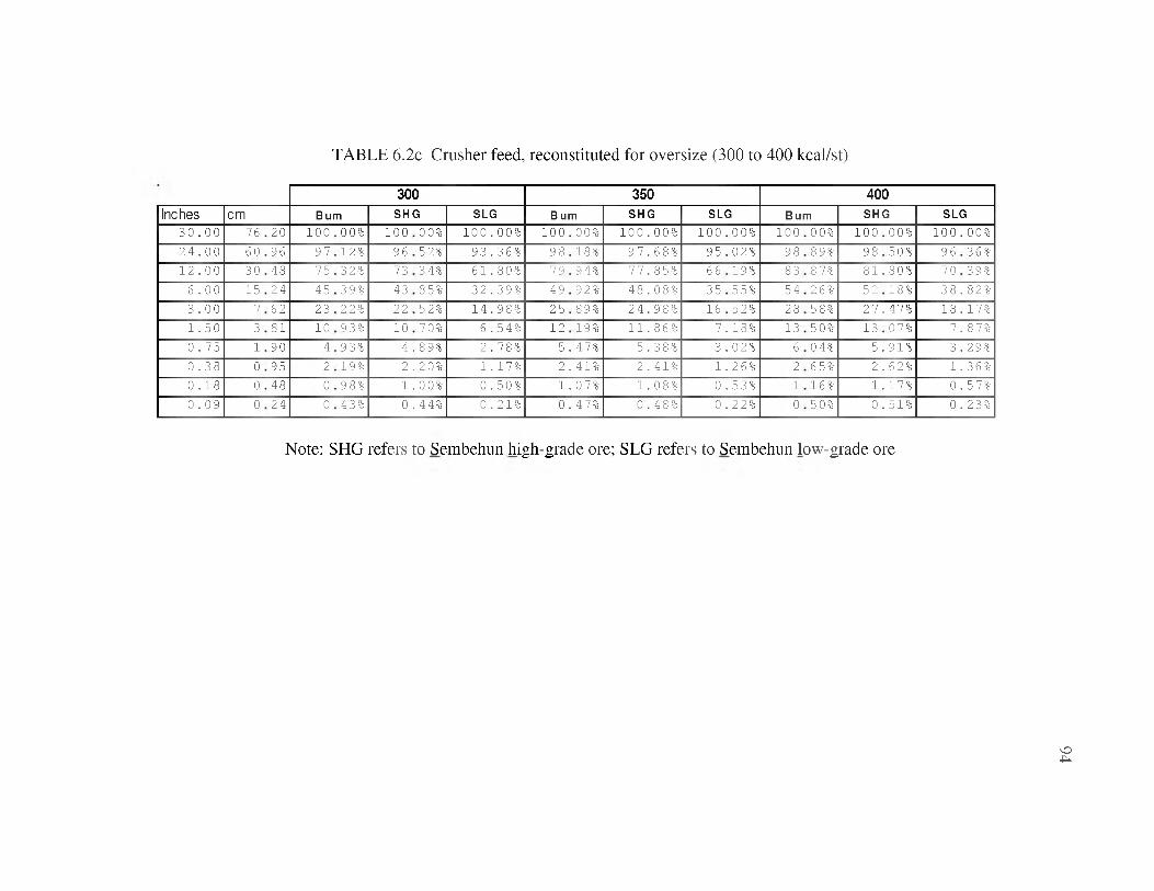
TABLE 6.2c Crusher feed, reconstituted for oversize (300 to 400 kcal/st)
300 350 400inches cm Bum SHG SLG B um SHG SLG Bum SHG SLG
3 0 . 0 0 76 20 1 0 0 00% 1 0 0 00% 1 0 0 . 00% 1 0 0 00% 1 0 0 . 00% 1 0 0 00% 1 0 0 00% 1 0 0 00% 1 0 0 . 00%
2 4 . 0 0 6 0 96 9 7 12% 9 6 52% 9 3 . 36% 9 8 18% 9 7 . 68% 95 02% 98 89% 98 50% 9 6 36%
1 2 . 0 0 3 0 48 75 32% 73 34% 6 1 . 80% 79 94% 7 7 . 85% 66 19% 83 87% 8 1 . 80% 7 0 39%
6 . 0 0 15 2 4 45 39% 43 85% 3 2 . 39% 49 92% 4 8 . 08% 3 5 55% 5 4 26% 5 2 18% 3 8 . 82%
3 . 0 0 7 62 23 22% 22 52% 1 4 . 98% 2 5 89% 2 4 . 98% 16 52% 28 58% 2 7 . 47% 1 8 . 17%
1 . 5 0 3 81 10 93% 10 70% 6 . 54% 12 19% 1 1 . 86% 7 . 18% 13 50% 13 07% 7 . 87%
0 . 7 5 1 90 4 93% 4 . 89% 2 . 78% 5 . 47% 5 . 38% 3 . 02% 6 04% 5 . 91% 3 . 29%
0 . 3 8 0 95 2 19% 2 . 20% 1 . 17% 2 . 41% 2 . 41% 1 . 26% 2 65% 2 . 62% 1 . 36%
0 . 1 8 0 48 0 98% 1 . 00% 0 . 50% 1 . 07% 1 . 08% 0 . 53% 1 16% 1 . 17% 0 . 57%
0 . 0 9 0 2 4 0 43% 0 . 44% 0 . 21% 0 . 47% 0 . 48% 0 . 22% 0 50% 0 . 51% 0 . 23%
Note: SHG refers to Sembehun high-grade ore; SLG refers to Sembehun low-grade ore
94

TABLE 6.3a Jaw Crusher Settings and features
95
Parameter ValueGap (m) 0.1778rmax 1.251Exponent, m 0.843Gape (mm) 1117.6 mm x 787.4 mm
(44 in. x 31 in.)Installed power (kW) 112
Source: Processing staff at W.U.S. Copper
TABLE 6.3b Settings and features of cone crushers
Setting Cone 1 Cone 2Open-Side Set (OSS) (meters) 127 mm (5 in.) 44.45 mm (1.75 in.)Closed-Side Set (CSS) (meters)
12.7 mm (0.5 in.) 6.35 mm (0.25 in.)
Installed power (kW) 298 298
Source: Processing staff at W.U.S. Copper

96
TABLE 6.3c Settings and features for Screen 1
Feature/Setting ValueNumber of decks of screen 3
Deck 1No. of screen panels in parallel 5Size of screen panels in parallel 31.75 mmModsim screen model used SCRNCrusher receiving screen oversize Cone 1
Deck 2No. of screen panels in parallel 5Mesh size of screen panels in parallel 4 screens: 9.525 mm;
1 screen: 28.575 mmModsim screen model used SCRNCrusher receiving screen oversize Cone 1 (from 4 screens); Cone 2 (from
one screen)
Deck 3No. of screen panels in parallel 5Size of screen panels in parallel 6.35 mmModsim Screen model used SCRNCrusher receiving screen oversize Cone 2
Source: Processing staff at W.U.S. Copper

97
TABLE 6.3d Settings and features for Screen 2
Feature/Setting ValueNumber of decks of screen 3
Deck 1No. of screen panels in parallel 5Size of screen panels in parallel 15.88 mmModsim screen model used SCRNCrusher receiving screen oversize Cone 1
Deck 2No. of screen panels in parallel 5Mesh size of screen panels in parallel 12.70 mmModsim screen model used SCRNCrusher receiving screen oversize Cone 1
Deck 3No. of screen panels in parallel 5Size of screen panels in parallel 6.35 mmModsim Screen model used SCRNCrusher receiving screen oversize Cone 2
Source: Processing staff at W.U.S. Copper

TABLE 6.4 The values inferred for the crushing simulation parameters
Crusher Parameter(s) Value
Cone 1Classification proportionality constants, a 1 and a 2 0 .5 ; 1 .85
The cum ulative breakage function, Bij 0 .6
Cone 2Classification proportionality constants, a 1 and a 2 0 .5 ; 1 .85
The cum ulative breakage function, B ij 0 .6
T A B L E 6 .5 The values of w ork index inferred for the crushing circuit
C rush er F so ( Hm) P 80 ( Hm) k 10 k Feed , tph OpK ilowatts
kW h/tOp. W ork
Index(Wi(o))
W i
Jaw 490,640 155,130 0.00111 0.01111 200.02 81 0.4050 36.44 29.15C o n e 1 148,090 10,300 0.00725 0.07255 241.2 101 0.4187 5.77 4.62C o n e 2 13,500 7,020 0.00333 0.03329 163.7 131 0.8002 24.04 19.23
W eighted average W i = 20.86 16.69
98

CHAPTER 7
SIMULATION OF THE CRUSHING OPERATION
7.1 Overview
Simulations were carried out to assess the influence of the blast-generated feed
particle size distributions on crushing outcomes. This simulation was done using
MODSIM. All simulations were performed on streams of material hypothetically mined
from three sources: Bom, Sembehun high-grade and Sembehun low-grade ore domains.
These ores were blended in the ratio 1:1:1. All materials in each blend were
hypothetically shot with the same specific energy. Each processed stream in this work
was uniquely identified by the energy factor with which that material was shot. Hence,
Bom ore that was shot with 100 kcal/st was blended with Sembehun high-grade ore and
Sembehun low-grade ore, each of which was shot with 100 kcal/st. This blend produced
Stream 100 kcal/st.
7.2 Simulation setup
The modeled/simulated crushing circuit configuration was the same as that used for
the parameter estimation exercise described in all of Section 6.2. The circuit included
one jaw crusher, two cone crushers (Cones 1 and 2), and 2 banks of screens, as shown in
Figures 1.1 and 6.1. The settings within the crusher circuit (including screens) are

outlined in Tables 6.3a 6.3b, 6.3c, and 6.3d, with further details provided in Appendix I.
The model parameters are outlined in Tables 6.4 and 6.5.
The main variable in each cycle of simulation was the particle size distribution of the
feed, dictated and identified by the blasting energy used to generate the particle size
distributions.
An important aspect of the crushing circuit is the feed particle size limit imposed by
the dimensions of the jaw crusher’s throat. The maximum crushable particle size is 0.76
meters (30 inches). Any size larger than this must be set aside and secondary-broken,
using a rock breaker. Usually, this re-break is done either at the crusher or at the mining
pit, and at an extra cost beyond the basic rates for blast fragmentation. The extra cost is
borne by the contractor, after an allowed maximum of 5% oversize.
This limitation to the features of the crushing circuit were taken into account in the
evaluation. To do this, the following assumptions were made:
i. The recovery of blasted ore to the crusher stockpile is 100%
ii. All oversize must be crushed to ensure all materials are fed into the crusher
iii. The distribution of particle sizes of daughter fragments produced from the broken
oversize is unknown, but may be assumed to follow the distribution of the original
on-spec feed size distribution (of size less than 30 inches). Thus, the mass
fractions of the feed in the sub-30 inch discrete size brackets were determined,
and used as the basis to prorate the feed oversize daughter fragment redistribution.
Accordingly, a new cumulative particle size distribution was inferred, accounting
for all initial undersize and all redistributed oversize.
100

iv. The percentage oversize in the original feed distribution is shown at the bottom of
Table 5.9a and 5.9b, and the new adjusted “true” feed particle size distribution to
the crusher is shown in Table 6.2a and 6.2b.
v. The cost of secondary breakage was reckoned, not against crushing costs, but
against blasting costs.
7.2.1 Results
Crushing simulation was carried out for all 11 oversize-reconstituted feed streams,
produced after “blasting” at the various energy factors and doing secondary breakage of
the oversize. Figure 7.1 is a plot of the size distributions of a number of the simulated
products from the range of feed distribution crushes. Importantly, it shows that there is
no difference in the particle size distribution produced, irrespective of the head feed
particle size distribution.
At a first glance, this result appears to be counter-intuitive. However, it does make
sense considering that each of the products only emerges if their particle sizes are finer
than the perforations of the same set of screens. Any larger size is recycled until it is
broken into a size smaller than the screen size.
7.2.2 Performance evaluation criteria
Beyond the particle size distribution, which has been shown above to be invariant
with the feed, the following criteria were used to evaluate the impact of blast energy
factor on crushing performance:
i. By-pass (fall-through) material and its potential impact on crusher throughput.
101

ii. The effect on crushing specific energy and crushing energy costs
It was not possible by the methods used in this work to assess the relative wear rates
of crusher linings, based on feed particle size distribution.
Tables 7.1a to 7.1h provide a summary of various results, including: crusher
throughput, percentage of fall-through material, power draw, specific energy, and costs.
7.2.2.1 By-pass (fall-through) material and throughput potential
As blasting energy intensity increases, the amount of fall-through material also
increases. Fall-through material is material which passes through the crusher without
being broken. The percentage of this kind of material in feed rises up to 55% at 400
kcal/st. Figure 7.2 is a plot of the percentage of fall-through material in blended crusher
feed. Theoretically, the benefit of this scale of fall-through is to aid potential throughput
capacity by allowing for scalping of the original feed and letting only larger sizes reach
the primary crusher. The scalped undersize should then bypass the primary crusher and
proceed to the secondary or tertiary crusher. Such an arrangement is particularly
important in situations where maximum throughput capacity is desired.
However, throughput capacity is not a challenge at W.U.S. Copper, as the crusher
generally operates up to a maximum of 12 hours a day and there is enough time slack to
crush further if such additional crushing is required. Adding a scalping facility to the
circuit would be making an unnecessary investment.
The other potential implication is for energy savings, as the amount of potential
bypass material should ideally not use up energy at the primary crusher.
102

This potential, too, does not seem to serve W .U.S. Copper well. The theory of the
crusher model is that material draws power only when the material is actually crushed.
No power is drawn from the passage of fall-through material. Thus, power saving
appears to have already been accounted for in the differences in energy draw at the
crusher. These differences are discussed further, in Section 7.2.2.2.
7.2.2.2 The effect on specific energy and energy unit costs
Figure 7.3 is a graph of specific energy values at the various stages of crushing. The
graph is based on the specific energy consumption data in Table 7.1d.
Specific energy at the crushing circuit appears to be affected only at the primary
crusher. The secondary and tertiary crushers show no significant differences in the
specific energies for the range of blast feed streams.
Even though there is some relative variation in specific energy at the primary crusher,
these variations do not bear significant economic advantage. The insignificance of the
economic advantage is owed to the fact that the differences in unit costs of crushing
energy ($/st) are negligible (see Table 7.1g). Between 100 kcal/st and 400 kcal/st, the
difference in unit cost of crushing energy is 1 cent. The monthly value of this difference
is approximately $510 (Table 7.1.h)
7.2.3 Conclusions about the impact on crushing
The economic or cost impact of blast intensity changes on this crushing circuit is not
significant. Expressed in terms of unit costs (of crushing specific energy), the cost
advantage for increasing blast energy factor is minimal. This situation is demonstrated in
103

Figure 7.4. However, the true importance of this marginal difference needs to be
explored further in terms of other costs that flow from the blast energy variations. These
impacts are evaluated collectively in Chapter 9.
104

Cum
ulat
ive
frac
tion
pass
ing
Particle Size (m icrons)
FIGURE 7.1 A plot of crushing product particle size distributions from ores blasted at 100, 140, 160, 180, 220, and 400 kcal/st. These results are superimposed on a plot of the actual mill feed (crusher product) particle size distribution. 105

% of
fee
d st
ream
60
55.04
142 100 140 160 180 220 250 280 300 350 400Blast Energy Factor (kcal/st)
FIGURE 7.2 Percentage of fall-through material in feed vs. blast energy factors 106

Crus
hing
Sp
ecifi
c En
ergy
(k
wh/
t)0.90
0.80
0.70
0.60
0.50
0.40
0.30
0.20
0.10
I Avg: 142
100
140
160
180
220
250
280
300
350
400
Jaw Cone 1 Cone 2
FIGURE 7.3 Variation of crushing specific energy with blasting energy factor
107

Unit
Cost
s of
cru
shin
g en
ergy
($
/t)
0.116
0.114
0.112
0.110
0.108
0.106
0.104
0.102
0.100100 140 160 180 220 250 280 300 350 400
Blast energy factor (kcal/st)
FIGURE 7.4 The variation of unit costs of crushing specific energy with blast energy factor
801

TABLES 7 (7.1a to 7.1h) Crushing rates, power draw, specific energy, and energy costs. T A B L E 7.1a: Feed rates through the crusher
C ru s h e r th ro u g h p u t (t/h )E F (k c a l/s t) A v g : 142 100 140 160 180 2 2 0 2 5 0 2 8 0 3 0 0 3 5 0 4 0 0
J a w 2 0 0 .02 2 0 0 0 2 2 0 0 0 2 2 0 0 0 2 2 0 0 0 2 2 0 0 0 2 2 0 0 0 2 2 0 0 0 2 2 0 0 0 2 2 0 0 0 2 2 0 0 0 2
C o n e 1 241 .00 2 4 0 2 0 2 4110 241 .40 241 .70 2 4 2 10 2 4 2 3 0 2 4 2 5 0 2 4 2 6 0 2 4 2 8 0 2 4 2 8 0
C o n e 2 163 6 0 163 8 0 163 6 0 16 3 6 0 263 5 0 16 3 5 0 16 3 6 0 263 6 0 163 7 0 163 9 0 26 4 2 0
T A B L E 7.1b: Percentage o f fall-through material at the primary crusher% F a ll-th ro u g h (b yp ass ) M a te r ia l
E F (k c a l/s t) 142 100 14 0 16 0 18 0 2 2 0 2 5 0 2 8 0 3 0 0 3 5 0 4 0 03 4 16 3 2 6 2 3 4 13 3 5 3 3 3 6 7 1 3 9 8 1 42 3 4 4 8 7 46 5 9 5 0 8 8 5 5 0 4
T A B L E 7.1c: Crusher p o w er drawC ru s h e r P o w e r D ra w (kW )
E F (k c a l/s t) A v g : 142 100 140 160 180 2 2 0 2 5 0 2 8 0 3 0 0 3 5 0 4 0 0J a w 81.0 8 3 .7 81.2 79 .7 78.1 74 .6 71.9 69.1 67.1 62 .0 5 6 .9
C o n e 1 101.0 101.0 101.0 101.0 101.0 101.0 101.0 101.0 101.0 101.0 101.0C o n e 2 131.0 132.0 131.0 130.0 131.0 131.0 131.0 131.0 132.0 132.0 133.0
T A B L E 7.1d: Crushing sp ecific energyS p ec ific E n erg y (k W h /t)
E F (k c a l/s t) A v g :1 4 2 100 14 0 16 0 18 0 2 2 0 2 5 0 2 8 0 3 0 0 3 5 0 4 0 0
J a w 20 40 20 42 20 41 02 40 0 3 9 0 3 7 20 36 20 35 20 3 4 20 3 1 20 28
C o n e 1 0 4 2 0 4 2 0 4 2 0 4 2 0 4 2 0 4 2 0 4 2 2 4 2 0 4 2 0 4 2 0 4 2
C o n e 2 20 8 0 02 8 1 20 8 0 2 7 9 2 8 0 20 8 0 20 8 0 02 8 0 20 8 1 02 8 1 02 8 1
T A B L E 7.1e: C rushing energy unit costsUnit C o s ts o f C ru sh in g E n erg y ($ / t )
E F (k c a l/s t) A v g : 142 100 140 160 180 2 2 0 2 5 0 2 8 0 3 0 0 3 5 0 4 0 0J a w 20 03 02 03 20 03 20 03 0 0 3 20 03 20 03 02 03 02 03 20 02 02 02
C o n e 1 0 0 3 0 0 3 0 0 3 2 0 3 2 0 3 2 0 3 0 0 3 2 0 3 2 0 3 2 0 3 0 0 3
C o n e 2 20 06 02 06 20 06 02 06 2 0 6 20 06 20 06 02 06 02 06 02 06 20 06
601

TABLE 7.1 (continued)
TABLE 7.1f: Crushing energy costs per hour
EF (kcal.st) Avg 142 100 140 160 180 220 250 280 300 350 400Jaw 4 4 5 4 5 9 4 4 6 4 3 7 4 2 9 4 0 9 3 9 5 3 7 9 3 6 8 3 4 0 3 1 2
Cone 1 5 5 4 5 5 4 5 5 4 5 5 4 5 5 4 5 5 4 5 5 4 5 5 4 5 5 4 5 5 4 5 5 4
Cone 2 7 1 9 7 2 4 7 1 9 7 1 3 7 1 9 7 1 9 7 1 9 7 1 9 7 2 4 7 2 4 7 3 0
Total 1 7 1 8 1 7 3 8 1 7 1 9 1 7 0 5 1 7 0 2 1 6 8 3 1 6 6 8 1 6 5 3 1 6 4 7 1 6 1 9 1 5 9 7
TABLE 7.1g: Net crushing energy unit costs
EF (kcal.st) 1 4 2 1 0 0 1 4 0 1 6 0 1 8 0 2 2 0 2 5 0 2 8 0 3 0 0 3 5 0 4 0 0
Average $/st 0 . 0 7 8 0 . 0 7 9 0 . 0 7 8 0 . 0 7 7 0 . 0 7 7 0 . 0 7 6 0 . 0 7 6 0 . 0 7 5 0 . 0 7 5 0 . 0 7 3 0 . 0 7 2
Average $/t 0 . 0 8 6 0 . 0 8 7 0 . 0 8 6 0 . 0 8 5 0 . 0 8 5 0 . 0 8 4 0 . 0 8 3 0 . 0 8 3 0 . 0 8 2 0 . 0 8 1 0 . 0 8 0
TABLE 7.1h: Crushing monthly energy costs (12-hr day operation)
EF (kcal.st) 1 4 2 1 0 0 1 4 0 1 6 0 1 8 0 2 2 0 2 5 0 2 8 0 3 0 0 3 5 0 4 0 0
Costs ($) 6 ,183 .71 6 ,2 56 .81 6 ,18 7.6 6 6 ,132 .75 6 ,126 .42 6 ,0 5 7 .2 7 6 ,0 0 3 .93 6 ,9 4 8 .6 1 5 ,9 2 8 .85 5 ,8 2 8 .10 6 ,74 7.10
110

CHAPTER 8
THE INFLUENCE OF FRAGMENTATION ON DRILLING AND BLASTING COSTS
AND LOADING AND HAULING PRODUCTIVITY
8.1 Overview
In this chapter, an account is given of the investigations carried out to assess the
effect of the degree of fragmentation on upstream stages of the mine-to-mill value chain.
These stages are drilling, blasting, loading, and hauling. For the mining operation under
review, it was found that fragmentation-induced variations in cost occur principally at the
drilling and blasting end, with adverse influences reaching the crusher in the form of the
oversize fragments. All costs arising from the various levels of oversize reaching the
crusher are reckoned to be extra costs of blasting.
The average stripping ratio at the mine is 5:1. For this reason, it is crucial to evaluate
the influences of blasting in waste as well as in ore. Blasting both materials could have a
significant effect on the overall economics.
8.2 Oversize rock and its implications for secondary breakage
and overall costs
Secondary breakage of both ore and waste are key considerations. Ore oversize
diameter threshold is at 76.2 cm (30 inches). Above this, blockage of the crusher throat

could occur. Waste oversize threshold is at 213.36 cm (84 inches). The limit is imposed
by the dimensions of the front end loader bucket.
From the Kuz-Ram predictions (see Section 5.4, and Table 5.9), there is a vast range
of oversize ore quantities (of between 41.9% and 0.4% ), corresponding to the full range
of blast energy factors involved. Maximum waste oversize is at about 10% (Table 5.10).
All oversize must be reduced by secondary breakage methods, so that the downstream
process can be carried out (crushing, in the case of ore, and dispatch to the waste dump,
in the case of the waste). The cost of this secondary reduction is necessarily an extended
blasting cost, and has been treated accordingly.
8.3 The effect of the degree of fragmentation on the costs
of drilling and blasting
The degree of fragmentation is directly related to the amount of explosive energy
infused into a unit mass or unit volume of rock. For a specified set of explosives, this
energy is directly related to the amount of explosives in a hole as well as to the number of
holes drilled and blasted per that unit volume or tonnage of ground. All conditions being
equal, the energy infused has a direct relationship to the unit cost of fragmentation.
8.4 Estimation of the costs of drilling and blasting
As part of this evaluation, the costs of drilling and blasting were estimated. The basis
of costing, as with the fragmentation prediction, was the use of ANFO as the main
explosive, and optimal initiation. Specific additional details of the basis of the estimates
are provided in the subsections on the costing of drilling (8.4.1) and blasting (8.4.2).
112
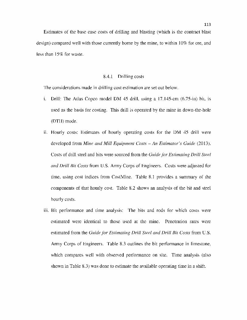
Estimates of the base case costs of drilling and blasting (which is the contract blast
design) compared well with those currently borne by the mine, to within 10% for ore, and
less than 15% for waste.
8.4.1 Drilling costs
The considerations made in drilling cost estimation are set out below.
i. Drill: The Atlas Copco model DM 45 drill, using a 17.145-cm (6.75-in) bit, is
used as the basis for costing. This drill is operated by the mine in down-the-hole
(DTH) mode.
ii. Hourly costs: Estimates of hourly operating costs for the DM 45 drill were
developed from Mine and Mill Equipment Costs - An Estimator’s Guide (2013).
Costs of drill steel and bits were sourced from the Guide fo r Estimating Drill Steel
and Drill Bit Costs from U.S. Army Corps of Engineers. Costs were adjusted for
time, using cost indices from CostMine. Table 8.1 provides a summary of the
components of that hourly cost. Table 8.2 shows an analysis of the bit and steel
hourly costs.
iii. Bit performance and time analysis: The bits and rods for which costs were
estimated were identical to those used at the mine. Penetration rates were
estimated from the Guide fo r Estimating Drill Steel and Drill Bit Costs from U.S.
Army Corps of Engineers. Table 8.3 outlines the bit performance in limestone,
which compares well with observed performance on site. Time analysis (also
shown in Table 8.3) was done to estimate the available operating time in a shift.
113

iv. Production analysis was done (Table 8.3), to determine the quantity of drilling
possible within the shift.
v. Unit costs of drilling were then calculated from the hourly costs, the drill
productivity, and the blast designs for each rock type. Tables 8.4 to 8.8 are
summaries of the development of these unit costs of drilling for both the ore and
waste rocks evaluated.
8.4.2 Blasting costs
The considerations made in blasting cost estimation were as follows:
i. Labor analysis, taking into consideration crew size and labor costs (Table 8.9).
ii. Time analysis, leading to a determination of available time for productive blasting
activity in a shift. The number of holes that can be blasted in that time is also
determined. Table 8.10 provides the analysis.
iii. Analysis of the production requirements. Annual production specified (ore and
3 3waste) was 114,683 m (150,000 yd ), at a stripping ratio of 5:1.
iv. The details and quantities of explosives and accessories per hole and per blast are
specified. Unit costs for the explosives were obtained from Dyno Nobel. Details
of this analysis are outlined in Tables 8.11 and 8.12.
The costs for drilling and blasting were combined and, for the ores of the three
categories, namely Bom, Sembehun high-grade, and Sembehun low-grade, are
summarized in Tables 8.13, 8.14 and 8.15, respectively. For each of these ores, the final
drilling and blasting costs, at all blasting energy factors, take into account both the basic
drill and blast costs and the extra costs of secondary breakage. The percentage of
114

oversize and undersize produced by the blast is presented. Table 8.16 outlines the mean
fragmentation cost for the ores, based on a ratio of 1:1:1. From these analyses, ore
oversize breakage potentially leads to increases over base case blasting costs of between
0.9% (Bom, at 400 kcal/st EF) and 355.7% (Sembehun low-grade, at 100 kcal/st EF).
For the contract design specifications for ore blasting, a net increase in blasting costs (per
ton) of up to 63% is expected.
Tables 8.17 and 8.18 provide summaries of drill, blast, and oversize reduction costs
for the two types of waste rock considered in the study, namely, limestone and
granodiorite, respectively. The size threshold for waste oversize characterization is
213.36 cm x 304.8 cm (84 inches x 120 inches), the limit being set by the capacity of the
loader bucket. Reduction of waste oversize is by secondary blasting, although a
mechanical breaker is also used. The unit cost of secondary reduction is $1.76/t
($1.60/st).
Secondary reduction is expected to be a major cost, for both ore and waste. To
explore the impact of secondary reduction, Table 8.19 shows the costs of primary
breakage, secondary breakage, and the overall cost of mining ore alone. Table 8.20 does
the same for waste alone. To visualize the relative impacts on both types of rock, Figures
8.1 and 8.2 have been developed respectively from the two tables.
In the ore graph (Figure 8.1), a summation of the primary and secondary breakage
costs produces a minimum in the region of 220 kcal/st. In the absence of waste, the 220
kcal/st design would produce the optimal blast, in terms of cost of ore fragmentation.
In the waste graph (Figure 8.2), the cost minimum is produced at 140 kcal/st. The
relative magnitudes of the breakage curves in Figures 8.1 and 8.2 demonstrate that
115

secondary breakage is not as significant a cost issue for waste as it is for ore. This
difference in importance of secondary breakage costs is understandable in the light of the
different thresholds at which oversize is reckoned for ore and for waste. For ore, all sizes
greater than 76.2 cm (30 inches) are considered oversize; for waste, the threshold is at
213.36 cm (84 inches).
A discussion of the overall impact of secondary breakage (and its implications for
primary breakage requirement) is not complete with the figures mentioned above. This is
because the average stripping ratio (5:1) has not been factored into the above scenarios.
These ratios are discussed in Chapter 9.
8.5 The influence of fragment size distribution on loading productivity
In order to evaluate and quantify a possible cause-and-effect relationship between
mining productivity and the particle size characteristics of the blasted material,
photographic methods, as described in Section 3.4.1, were used to sample fragmentation
at the mining face at W.U.S. Copper’s Sembehun Pit. Corresponding time-and-motion
data were collected specifically for the loading segment of the mining activity.
Fifteen sets of photos were shot across a blasted face of ore and waste (an average of
four photos per set). Each set of photos was shot across about 20 m (66 ft) of the mining
face. On the average, this width of face had enough rock for about five truckloads of a
CAT 777 truck. The set of four photos was considered enough to assess the
fragmentation across that face and to aid the evaluation of the impact of the particle size
distribution on loading in that relatively small area.
116

To take a photo, two buckets were positioned for scale in the muck pile, about 4 m
apart. One bucket was lined up behind the other to provide depth of view. After the
image of a desired area had been captured in this manner, the buckets were relocated, and
more photos taken.
Using a split-second stop watch, loading cycles from the photographed pile were
timed. Each cycle started when the front end loader’s bucket bit against the material in
the stockpile, and ended when the material had been scooped, swung, and discharged into
the truck, and the bucket teeth set against the face again to scoop the next load.
Each set of photos was processed in Split Desktop™ to estimate the particle size
distribution. Figure 8.3 is a sequence of photos demonstrating various stages of image
processing in Split Desktop™. Figures 8.4 and 8.5 are examples of the results obtained
from the photo processing.
From the results of the analysis of each set of photos, the top size, 95%, 80%, 50%,
and 30% passing sizes were extracted for all 15 sets of data. Table 8.21 is a summary of
these data, including average size of load and single-pass load cycle of the CAT 992
loader.
8.6 Evaluation of loader cycle/productivity versus fragment
size distributions
Using the data in Table 8.21, a statistical evaluation was carried out in Minitab™.
Principally, linear regression relationships were explored between each of the size
thresholds represented in the table (topsize, 95%, 80%, 50%, and 30% passing sizes) and,
117

separately, average cycle time for a single pass, and pass load (short tons). Simple linear
regressions and multiple linear regressions were carried out.
In addition to the regular regressions that were run, a routine for stepwise regression
in Minitab™ was used to rigorously assess the possibility that one or more of the
available predictors might yield a significant regression.
Furthermore, a variety of different functional forms were explored, including
exponential and logarithmic relationships, with subsequent linearization of the
transformed values.
8.7 Results of statistical analysis
Figure 8.6 is a graph of cycle time vs. topsize, and Figure 8.7 is a graph of cycle time
vs. mean size. The result (produced in Minitab™) of the regressions of cycle time on the
entire set of predictors is presented in Figure 8.8. The criteria of interest in evaluating the
regression equation are the F-statistic (f0 ) and the coefficient of determination, R2 (both
shown within the ellipses in Figure 8.8). The hypothesis in the evaluation of the
regression results is that the predictors (top size, F 80, F50, etc.) have no significant impact
on the loading cycle time. The alternative hypothesis is that the predictor(s) do(es) have
an effect on the outcome. In the case of a simple linear regression, when f0 > fa,i,n-2, the
null hypothesis is rejected and the predictor does significantly affect the response
variable. Hence, the model may be used to dependably predict the response. For
multiple linear regression, the criterion for rejection is that: f0 > fa,k,n-p (Montgomery and
Runger 2011).
118

However, in all cases considered, fa,i,n-2 and fa,k,n-p obtained from the F distribution
tables have been greater than 3, which is greater than all values of f0 (shown only as F, in
the Minitab™ results). These results lead to an acceptance of the null hypothesis,
indicating that the various factors (top size, mean size, etc.) may not be used for the
desired prediction purposes.
In all cases of the simple and multiple regressions, the value of R2 shown in the
results was low (most of them well below 50%), hence, indicating a poor fit of the model
to the data.
The aim of the stepwise regression mentioned in Section 8.9 was to evaluate each of
eleven possible predictors (including transforms and aggregates of some of the original
variables) for their potential to validly predict either the cycle times or the size of the
bucket load or to predict both. Figure 8.9 shows the result of the stepwise regression that
was run between cycle time and 11 predictors. The result was that no variables passed
the statistical criteria, and none of them could be “entered” into or used in the model to
predict the cycle time. A similar result was obtained for the investigation of the
prediction of mass in the bucket load.
Figure 8.10 is a plot of the residuals in the regression between cycle time and the
various candidate regressors. The plot shows that the errors are normally and
independently distributed with a mean of zero and a variance equal to the variance of the
data. Normality and randomness are used as a test for the adequacy and validity of the
regression. These residuals refer to the results in Figure 8.8.
In spite of the adequacy of the model (as demonstrated by the normality of the
various plots), there was, however, no significant or meaningful relationship between the
119

particle size distribution of the blasted rock pile and either the loader cycle time (which
impacts the loading speed) or the size (load) of the pass.
8.8 Implications
The conclusion is drawn that, if the fragment size distribution has no significant effect
on the loader cycle time, then that fragment size distribution should not have any effect,
either, on the haulage cycle times. No other data were collected to monitor such a
relationship, nor could any other be conceived with reasonable chances to demonstrate
impact better than the fragmentation data already evaluated.
Indeed, while this outcome does appear to challenge conventional wisdom, it may,
however, actually bring sharply into focus an element that is generally disregarded when
mine-to-mill issues are being discussed. This element is the human factor. It is
conceivable that a loader operator’s performance does rise and fall during an operating
session, and that this performance may be susceptible to influence by extraneous factors,
including operator competence and general circumstances. This explanation was not
explicitly investigated. However, its validity is considered an important possibility.
In pursuing methods to evaluate the fragment size distribution and loading
productivity relationship at an earlier stage of the research, discussions were held with
John Floyd, of Blast Dynamics. Floyd had previously developed a system (ProDig) for
characterizing this relationship, but appears to have abandoned the use of that system
when his findings at several operations around the world demonstrated that “there is more
deviation in cycle time due to operator experience than that related to fragmentation”
(Floyd, 2014, pers. comm., August 4, 2014).
120

8.9 Estimation of wear and tear arising from degrees of
rock fragmentation
Wear and tear is considered a major component of the effect of blasting on an
operation’s economic bottom line. However, it was not possible in this work to directly
relate wear and tear effects to blasting energy or blast-generated particle size distribution.
Certainly, such a relationship, if it exists, would be an important one to investigate.
121

Cost
($/s
t)
Blast Energy Factor (kCal/st)
FIGURE 8.1 A plot of ore breakage costs versus energy factor
122

Cost
s ($
/st)
Blast Energy Factor (kcal/st)
FIGURE 8.2 A plot of waste breakage costs against energy factor
123

124

FIGURE 8.3 (CONTINUED)
125

C o m b i n e d I M G _ 0 9 2 8 I M G _ 0 9 2 9 I M G _ 0 9 3 0 I M G _ 0 9 3 1 I M G _ 0 9 3 2 I M G _ 0 9 3 3S i z e [ i n ] % P a s s i n g % P a s s i n g % P a s s i n g % P a s s i n g % P a s s i n g % P a s s i n g % P a s s i n g
7 5 100 1 0 0 1 0 0 1 0 0 1 0 0 100 1 0 05 0 99 . 8 8 1 0 0 1 0 0 99 . 4 9 1 0 0 100 1 0 03 0 79 . 4 7 7 5 . 1 2 71 . 2 7 83 . 8 8 81 . 6 3 7 4 . 68 84 . 3 125 70 . 5 1 6 4 . 5 2 61 . 4 4 77 . 8 5 73 . 7 6 6 3 . 38 75 . 1 41 5 48 . 7 1 4 4 . 5 1 40 . 6 2 60 . 0 1 57 . 3 8 4 0 . 95 50 . 8 71 0 37 . 7 3 3 4 . 5 1 27 . 7 5 50 . 7 8 49 . 8 5 3 1 . 39 36 . 8 1
8 33 . 7 5 2 9 . 5 22 . 7 4 47 . 5 7 46 . 86 2 8 . 34 32 . 7 76 30 . 1 3 2 4 . 8 2 18 . 5 7 43 . 4 1 44 . 4 1 2 5 . 85 30 . 0 14 25 . 0 5 1 9 . 1 8 13 . 7 9 37 . 0 3 39 . 7 5 1 9 . 95 26 . 9 32 17 . 7 8 1 2 . 3 4 7 . 9 3 28 . 1 8 31 . 9 2 12 . 8 19 . 7 91 1 2 . 8 7 . 9 3 4 . 5 6 21 . 4 2 25 . 6 1 8 . 2 14 . 5 2
0 . 7 5 11 . 2 1 6 . 5 9 3 . 6 2 19 . 1 1 23 . 3 6 6 . 82 12 . 7 70 . 5 9 . 3 2 5 . 0 8 2 . 6 2 16 . 2 6 20 . 5 2 5 . 25 10 . 6 4
0 . 3 8 8 . 2 4 . 2 2 2 . 0 8 14 . 4 9 18 . 7 1 4 . 36 9 . 3 50 . 2 5 6 . 8 6 3 . 2 5 1 . 5 12 . 3 2 16 . 4 3 3 . 35 7 . 7 80 . 1 9 6 . 0 5 72 1 . 1 9 10 . 9 7 14 . 9 7 2 . 77 6 . 8 30 . 0 8 4 . 2 1 1 . 5 4 0 . 5 9 7 . 7 7 11 . 3 6 1 . 58 4 . 6 2
C o m b i n e d I M G _ 0 9 2 8 I M G _ 0 9 2 9 I M G _ 0 9 3 0 I M G _ 0 9 3 1 I M G _ 0 9 3 2 I M G _ 0 9 3 3% P a s s i n g S i z e [ i n ] Si z e [i n ] Si z e [ i n] S i z e [ i n ] S i z e [ i n ] S i z e [i n] Si z e [i n ]F 1 0 0 . 5 8 1 . 4 4 2 . 6 7 0 . 1 5 0 . 0 5 1 . 36 0 . 4 4F 2 0 2 . 5 4 4 . 2 7 6 . 7 2 0 . 8 4 0 . 4 6 4 . 02 2 . 0 5F 3 0 5 . 9 4 8 . 2 10 . 8 8 2 . 3 4 1 . 6 4 9 . 13 5 . 9 9F 4 0 11 . 0 8 1 2 . 5 2 14 . 7 4 4 . 8 7 4 . 0 8 1 4 . 53 11 . 2 8F 5 0 15 . 5 8 1 7 . 8 4 18 . 9 7 9 . 5 3 1 0 . 1 19 . 3 14 . 6 9
F 6 0 19 . 9 3 2 2 . 8 1 24 . 1 6 14 . 9 9 16 . 6 9 2 3 . 58 18 . 3 6F 7 0 24 . 7 2 2 7 . 6 2 29 . 3 9 20 . 0 9 22 . 6 1 2 7 . 85 22 . 4 7F 8 0 30 . 3 1 3 2 . 2 9 34 . 1 9 26 . 7 2 28 . 9 9 32 . 5 27 . 6 3F 9 0 37 . 1 3 3 9 . 5 39 . 3 3 35 . 9 1 35 . 3 8 3 8 . 31 34 . 8 5F 9 5 42 . 0 6 4 3 . 9 9 43 . 3 4 42 . 2 2 39 . 4 7 4 1 . 74 40 . 6 2T o p s i z e ( 9 9 . 9 5 0 . 3 8 4 9 . 2 48 . 4 4 50 . 9 3 49 . 2 4 4 5 . 84 4 7 . 5
C o m b i n e d I M G _ 0 9 2 8 I M G _ 0 9 2 9 I M G _ 0 9 3 0 I M G _ 0 9 3 1 I M G _ 0 9 3 2 I M G _ 0 9 3 3F i n e s C u t o f f [ i n ] 4 . 4 6 6 . 0 4 5 . 3 5 7 . 06 5 . 4 8 6 . 03 4 . 6 2F i n e s F a c t o r 50 50 50 50 50 50 50
FIGURE. 8.4 A screenshot example of the fragment size distribution results from blast image processing in Split Desktop ™
(1 inch = 2.54 cm)
126

CDCcn c/) CO
CL
d>oix>
CL
100
80
60
40
20
P n m h i n p r l
/
—I \ 1 H -----1--- —H- 1----- ---1-- l-Hh-M • - • • t0.0 0.1 1.0
Size[in]10.0 100.0
S P L I T ^ D E S K T O P s p u i m w s
FIGURE. 8.5 A screenshot example of the fragment size distribution graph, obtained from blast image processing in Split Desktop™
(1 inch = 2.54 cm)
127

Sing
le Pa
ss
Load
Cy
cle
(sec
s)60.00
50.00
40.00
30.00
20.00
10.00
♦ ♦ ♦
y = 0.0196x + 43.684 R2 = 0.0062
—i—20 40 60 80
Fragment Top Size (inches)
100 1200
FIGURE 8.6 Regression plot of loading cycle time vs. top size.
1 inch = 2.54 cm 128

Sing
le Pa
ss
Load
Cy
cle
(sec
s)
60.00
50.00
40.00
30.00
20.00
10.00
♦ ♦
—i—16
—i—18
—i 208 10 12
Mean Fragment Size (inches)
140 4 6
FIGURE 8.7 Regression plot of cycle time vs. mean size
1 inch = 2.54 cm
129
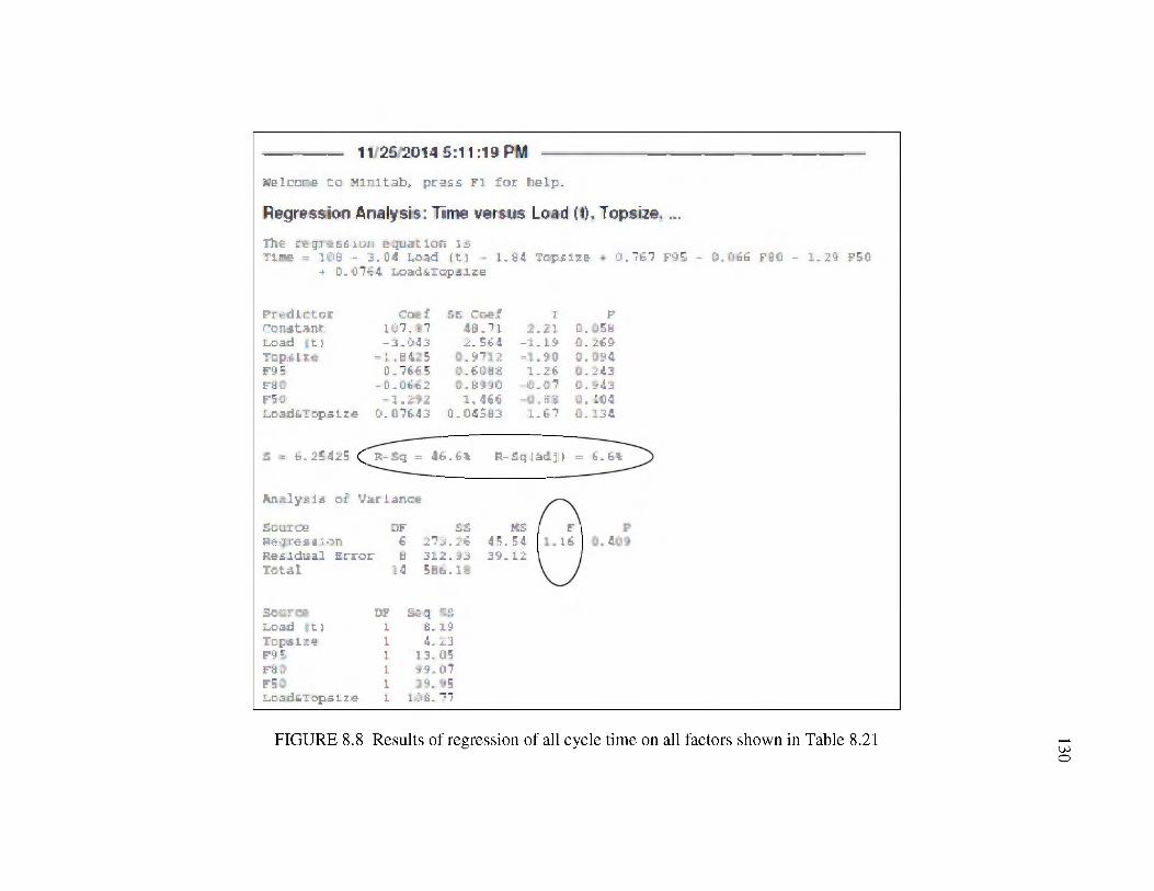
11 25 2014 5:11:19 PM
K E l c c r i t c M l n l t a b j . pc-2 S£ F I f o r h e l p .
Regression Analysis: Time versus Load (0, Topsii^ ...T he t e g r " sri Ibf ; e z j u i t l c J i 1 bT l p e = 1 0 6 - 3 . 0 4 L o a d [ t ! - l . $ 4 T a p j s i i e
■+ D - 0 7 * : 4 L o a d & r o p = l z e0.767 F95 - 0,066 F60 - l.iS F5C
P r e d i c t o r Ceef i s c « ? f T pConstant 1 0 7 , : 7 46 .7 1 2 .21 0,,65HLoad ( t :■ - 3 . 0 1 3 2, £6 4 -1 .1 9 0. 26&Top i I z c - i .u 4 :5 0 . &71Z -1 .9 0 0.0 9 4F9B 0 .7 66 5 o . t c u s 1 -26 j . 243ra& -D .D 6 6 2 0 . U990 -0 . Q l 0. L>iJFS0 - I . 1^2 1. 4 6 6 -0 . BE o. 404■loadfiTopslze 0 .0 7 6 4 3 Q-04£b3 1 .61 0. 134
= G.2S425 £ R-Sq = i t . Ct R- S q t a d j } = S. 61
Analye14 of Variance
£dui:Cb OF ££ USRegression 6 271.26 45.54Residual E rro r fl 3 1 2 .9 3 39*12 Total Id 5B6.18
I16 40'
Source L o a d [ t ) Tops-iis FI 5 F3D F50L o ad tT o p slie
OF Ecq S3 B. i& A. 23
13,05 99.07 39.45
1 0 6 . 1 7
FIGURE 8.8 Results of regression of all cycle time on all factors shown in Table 8.21 130

FIGURE 8.9 The results of stepwise regression on all factors shown in Table 8.21 131

Normal Probability Plot Versus Fits
re3■o'552
10
5
0
-5
-1035
Residual40 45 50
Fitted Value
Histogram Versus Order
4.8
£ 3.6 c e& 2.4 e
1.2
0.0■10.0 -7.5 -5.0 -2.5 0.0 2.5 5.0 7.5
Residual Observation Order
FIGURE 8.10 A plot of the residuals from the regression of cycle time on various factors
132

TABLE 8.1 Hourly operating costs for a DM 45 drill rig
O verhaul M ain ten an ce Operating T o tal
P arts
($ /hr)
L abor
($ /hr)
P a rts
($/hr)
La bo r
($ /hr)
D ie se l
($ /hr)
Lube
($ /hr)
W ear
P a rts
($ /hr)
To tal
($ /hr)
Driller's net
W ag es+ benefits
($/hr)
Grand T o ta l (excl.
ow nership) ($/hr)
718 6 77 5 3 7 5 5 4 5159 10 5 5 34 2 7 121 .77 40 71 162 .43
(Source: Infomine USA Inc. Costmine Division 2013; U.S. Army Corps of Engineers 2009)
133

TABLE 8.2 Development of costs for drill steel and bits
S t e e l D r i l l b i t
Feet drilled/hole (approx) 2 4
Ro ds 2
$ /ft/ro d 0 0 1 7 5
Adj. Facto r 15
$ / f t d r i l l e d 0 . 0 2 6 2 5 0 .19P enetratio n rate (ft/hr) 127 5 127 5
$ / h r = f t / h r * $ / f t 3 3 4 6 8 7 5 2 4 2 2 5
To tal $ /hr (2006 co s ts ) 2 7 . 5 7 1 8 7 5
2006 Co st Index 186 5
2014 Cos t Index 2 3 1 8
2014 Cos t of wear items ($) 3 4 . 2 7
Source: U.S. Army Corps of Engineers 2009
134

TABLE 8.3 Bit performance, time analysis and drill productivity in limestone
Penetration 2 125 feet/m inTime analysis Ho le length 23 9 3 7 5 ft/ho le
Drilling Rates: 311 3 mins/holeLength o f shift 10 hrs/shift Adding pipe 3- mins/hole
Less: Pulling pipe 03 5 mins/holeStart up and Delays 3 25 hrs/shift M aneuvering Time 33 0 mins/holeLunch 0 50 hrs/shift Leveling Time 31 0 mins/holeM ajor moves - hrs/shift Tota l Drill Cycle 15 3 mins/holeM isc Delays 03 25 hrs/shift 30 26 hr/holeT o ta l Delays 1.0 0 hrs/shift
Available Drilling time 39 00 hrs/shift Drill P roductivi ty 3 31 holes/hour334 25 holes/shift
135

TABLE 8.4 A summary of the development of unit costs of drilling for Bom ore
EF (kwh/st) DO 12 9 14 O 16 O 18 O 22O 2 5 0 28O 3 0 0 35O 4OO
Bench height (L) (ft) 2 0 0 0 9 920.00 920.00 2 0 0 0 2 0 0 0 2 0 0 0 2 0 0 0 2 0 0 0 2 0 0 0 9 0 0 0 9 0 0 0Hole length (ft) 2 3 9 4 9 923.94 923.94 2 3 9 4 2 3 9 4 2 3 9 4 2 3 9 4 2 3 9 4 2 3 9 4 9 3 9 4 2 3 9 4Burden, (B) (ft) 1 5 9 2 14 0 1 913.45 912 58 1186 10 .73 10 0 7 9 5 1 99 98 51 97 96Spacing, (S) (ft) 18 3 0 1612 915.47 194 47 13 .64 12 3 4 1158 10 9 4 10 5 7 99 78 9 15yd3/hole 215.79 167 2 8 9154.14 134 8 7 119 8 9 98 0 9 86 3 2 77 0 7 7 1 9 3 9 1 6 6 5 3 9 5yd3/shift 7 3 9 1 . 7 5 5 ,7 3 0 0 4 5 2 7 9 8 2 9,619 8 4 4,106 5 3 3 3 5 9 8 9 2 ,9 5 6 .70 2 , 6 3 9 9 1 2 , 4 6 3 9 2 9,111 9 3 1 8 4 7 9 4yd3/hr 8 2 1 3 1 6936.67 9586.65 513 3 2 9 5 6 2 8 3 7 3 3 2 3 2 8 5 2 9 9 3 3 2 2 7 3 .77 2 3 4 6 6 2 0 5 3 3s t/hr 2 2 6 1 8 7 91,753.39 1615 6 2 9,413 £ 7 1 2 5 6 .60 1 0 2 8 12 9 0 4 7 5 8 0 7 8 1 7 5 3 9 6 6 4 6 2 5 5 6 5 .47$ /yd3 09.20 09.26 09.28 90 32 9 3 6 09 44 90 49 90 5 5 90 59 90 69 0 .79$/st 90.07 90.09 90 10 90 11 0 13
^309 0 18 90 20 90 22 90 2 5 0 2 9$/t 09.08 1090 09 11 90 13 0 14 90 90 20 90 22 90 24 90 28 90 32
136

TABLE 8.5 A summary of the development of unit costs of drilling for Sembehun high-grade ore
EF (kwh/st) 100 142 14 0 160 180 220 250 280 300 350 400
B en ch height (L) (ft) 2 0 0 0 2 0 0 0 2 0 0 0 2 0 0 0 2 0 0 0 2 0 0 0 2 0 0 0 5 0 0 0 5 0 0 0 2 0 0 0 2 0 0 0Hole length (ft) 2 3 9 4 2 3 9 4 2 3 9 4 2 3 9 4 2 3 9 4 2 3 9 4 2 3 9 4 5 3 9 4 2 3 9 4 5 3 9 4 2 3 9 4Burden, (B ) (ft) 16 7 1 14 0 2 14 12 13 2 1 12 4 5 511 26 10 5 7 59 98 59 6 5 8 9 3 8 3 5Spacing, (S) (ft) 19 2 1 16 12 16 2 4 515 19 14 3 2 512 95 512 15 11 .48 1109 10 2 7 59 6 1yd3/hole 2 3 7 7 5 167 .43 169 8 2 148 5 9 532 0 8 108 0 7 9 5 10 8 4 9 1 79 2 5 6 7 9 3 5 9 .44yd3/s hift 8,143 7 9 5 , 7 3 5 0 6 5 8 1 6 9 9 5 , 0 8 9 8 7 4 5 2 4 3 3 3 , 7 0 1 .72 3 2 5 7 5 2 5 , 9 0 8 5 0 2 ,714 6 0 5 3 2 6 8 0 5 , 0 3 5 9 5yd3/hr 9 0 4 8 7 6 3 7 2 3 6 4 6 3 3 5 6 5 5 4 5 0 2 7 0 41130 3 6 1 9 5 3 2 3 17 3 0 1 6 2 2 5 8 5 3 2 2 6 2 2s t/hr 2 , 2 6 1 8 7 1 5 9 2 8 7 1615 6 2 1,413 6 7 1 2 5 6 6 0 1 0 2 8 12 9 0 4 7 5 8 0 7 8 1 7 5 3 9 6 6 4 6 2 5 5 6 5 .47
$ yd Q- 0 18 0 2 5 0 2 5 0 2 9 5 3 2 5 .40 0 .45 0 5 0 0 5 4 0 6 3 0 7 2
s$ 0 0 7 0 10 0 10 0 11 0 13 0 16 0 18 0 2 0 0 2 2 0 2 5 0 2 9$/t 0 0 8 0 11 0 11 0 13 0 14 0 17 0 2 0 0 2 2 0 2 4 0 2 8 0 3 2
137

TABLE 8.6 A summary of the development of unit costs of drilling for Sembehun low-grade ore
E F (kwh/st) 100 155 140 160 180 220 250 280 300 350 400
B e n c h height (L) (ft) 2 0 0 0 90 00 20 00 20 00 20 00 20 .00 90 00 20 .00 20 00 90 .00 20 00
Hole length (ft) 2 3 9 4 93 94 23 9 4 23 9 4 23 9 4 23 9 4 93 9 4 23 9 4 23 9 4 93 9 4 23 9 4
Burden, (B ) (ft) 17.4 4 194 00 914 74 913 78 13 00 911 75 191 03 10 .42 10 0 7 99 32 89 72
Sp acing , (S ) (ft) 2 0 0 5 196 10 916 9 5 15 8 5 14 9 4 913 52 912 68 911.98 91 58 9 9 190 72 10 03
yd3/ho le 258 9 5 167 07 984 9 7 16185 143 86 9117 71 103 58 92 .48 86 32 93 99 64 .74
yd3/shift 8 8 7 0 10 5,722 65 6 3 3 5 .79 5 ,543 8 1 4,927 83 4 ,03186 9,548 0 4 3,167 8 9 2,956 .70 9 ,534 31 2 2 1 7 53
r/h
id 985 5 7 635 85 703 98 615 98 5 47 5 4 947 98 394 23 9351.99 328 52 2 8159 946 39
s t/hr 2 2 6 1 8 7 91,459 27 1615 62 1413 6 7 9,256 60 1028 12 904 7 5 807 81 753 96 646 2 5 565 .47
$/yd3 9 16 90 26 09 23 90 26 0 30 90 36 0 .41 0 .46 0 .49 90 58 90 66
$ /s t 90 07 90 11 09 10 90 11 0 13 90 16 0 18 0 20 90 22 90 25 90 29
$/t 09 08 90 12 90 11 90 13 0 14 90 17 90 20 0 22 0 2 4 9 9 90 28 90 32
138

l o ooo .0003 948.93
10 2767 94
2 3 2 7 03258 56565 47
0 1 T02 9 "0 1 2
TABLE 8.7 A summary of the development of unit costs of drilling for limestone
10020 00 23 94 17 86
20 54 071.74
162.5 140 160 180 220 250 280 30000 oo 20 00 00 oo 20 00 20 00 20 00 20 00 20 00223 94 23 94 223 94 23 94 23 94 23 94 23 94 23 94
04 01 15 09 04 12 13 31 12 04 1130 10 67 10 31
11106 17 36 06 24 15 31 13 85 12 99 12 27 1186167 23 194 10 169 84 150 97 123 52 108 70 97 05 90 58
0,728 08 6648 67 5817 58 5,17118 4 2 3 0 9 7 3,723 25 3 3 2 4 3 3 3,102 71636 45 038 74 646 40 574 58 470 11 013 69 069 37 044 .75
0,39192 1615 .62 0413 .67 125660 1028 12 004 75 807 81 "753 960 26 0 22 0 25 0 28 0 35 0 39 0 44 0 470 12 0 10 0 11 0 13 0 16 0 18 0 20 0 220 13 0 11 0 13 0 14 0 17 0 20 0 22 0 24
9308 13 1034 24 226187
0 ¥ 0 0 7 0 0 ?

TABLE 8.8 A summary of the development of unit costs of drilling for granodiorite
EF (kwh/st) 100 1 64 .5 140 160 180 2 2 0 2 5 0 2 8 0 3 0 0 3 5 0 4 0 0B en ch height (L) (ft) 20 j00 20 00 20 0 0 20 00 20 .00 20 00 20 0 0 20 00 20 00 20 0 0 20 00Ho le Length (ft) 23 9 4 223 94 23 9 4 23 94 23 94 23 94 23 9 4 23 94 23 94 23 9 4 23 94Burden, (B ) (ft) 27 9 7 24 01 25 19 214 2 1 23 .40 12 12 11 3 7 2 120 74 2 38 229 6 1 28 99Spacing, (S ) (ft) 20 6 7 2 126 11 17 .47 126 34 25 .40 13 93 23 0 7 2 122 35 2193 211.05 20 33yd3/ho le 2 75 14 167 26 196 5 3 2171.96 152 .85 125 0 6 2110 05 28 26 2171 78 61 68 .78yd3/sh ift 2,424 .48 5 ,729 17 2 ,73177 22,890 3 0 22,235 .82 4 2 8 3 86 2 ,769 .79 2 3 6 5 8 9 3,14149 2 6 9 2 .71 2 3 5 6 12yd3/hr 2,047 16 6 36 57 747 9 7 654 .48 581.76 4 7 5 9 8 418 8 7 373 99 349 0 5 29 9 19 261 7 9s t/hr 2 2 6 1 8 7 2 3 7 5 00 1615 6 2 2,413 67 2 256 .60 2028 12 904 .75 807 81 753 96 646 2 5 5 65 .47
3d/y&
0 16 0 26 20 22 20 25 0 28 220 34 20 39 2 20 43 2 20 47 20 54 20 62$ /s t 2 20 07 0 12 0 10 20 11 0 13 0 16 20 18 2 20 20 2 20 22 20 25 20 29$ /t 2 20 08 0 13 0 11 20 13 0 14 0 17 20 20 2 20 22 2 20 24 20 28 20 32
140

TABLE 8.9 Blasting labor analysis
141
Ro le QtyW a g e s &benefi ts
( $ / h r )H o u r s C o s t ($ / d a y )
F o r e m a n 1 24 8 192P o w de r M e n 2 20 8 320Driver s 1 20 8 160
To tal 6 7 2N o t e : N o . o f T e a m s = 1
TABLE 8.10 Time analysis for blasting
A v a i la b le t ime A n a ly s i sH ours p er shift ho urs 8
L ength o f shift mins 480
Startup mins 55
Lunch mins 20
M is c . delays mins 55
Shutdow n mins 15
A v a i la b le t ime mins /s hift 385
Tim e Utilization Analysis
C o n n e c t tim e (@ 1 min/hole) mins 140
L oad tim e (@ 1 min/hole) mins 140
C lear pit mins 55
Sh o o t and c le a r s h o t mins 30
R/T m agazine mins 55
Lo ad tim e @ m agazine mins 55
T o t a l t ime p er sh i f t mins 385

142
TABLE 8.11 Unit costs of explosives products
Ite m Unit V alu eExplo s ive A N F OExplo s ive C o s t $ / lb 0 2 5B o o s t e r T y pe lb 1B o o s t e r C o s t $ e a 6 0 0S n a p Line $ e a 5 5 0N o n e l D e t o n a t o r s $ e a 6 5 0
Source: DynoNobel
TABLE 8.12 Development of the cost of a single blast
B as is : N O N E L In i t i a t io nIte m Unit Qty Uni t c o s t ($ /lb) C o s t ($ )
P o wder (Explo s ive) lb 2 0 5 9 3 0 2 5 5,148 2 3B o o s t e r s ea 140 6 8940 00N o n e l d e to n a to r ea 140 6 5 910 0 0Sn ap line ea 119 5 0 7 9 0 3 3 3Any o ther (det cord ) ea 9 ,000 0 124 2 4 8 0 0Initiating c a p (100 ft) lo t 1 12 912 00T o ta l : E xp lo siv es and a c c e s s o r i e s 7 ,7 61 .5 6L a b o r S e t 1 672 9 7 2 0 0To ta l c o s ts ($ ) 8 ,4 3 3 .5 6

TABLE 8.13 A summary of the combined drilling, blasting, secondary breakage and mean blending fragmentation costs for Bom ore
E xplosive energy (kcal/st) 1 0 0 1 2 9 C o n t r a c t 1 4 0 1 6 0 1 8 0 2 2 0 2 5 0 2 8 0 3 0 0 3 5 0 4 0 0
Drill 0 . 0 7 0 . 0 9 0 . 1 0 0 . 1 1 0 . 1 3 0 . 1 6 0 . 1 8 0 . 2 0 0 . 2 2 0 . 2 5 0 . 29
Blast 0 . 1 0 0 . 1 4 0 . 1 5 0 . 1 7 0 . 1 9 0 . 2 2 0 . 26 0 . 2 9 0 . 3 1 0 . 3 6 0 . 4 1
Total 0 . 1 7 0 . 2 3 0 . 2 5 0 . 28 0 . 3 2 0 . 3 8 0 . 4 4 0 . 4 9 0 . 5 2 0 . 6 1 0 . 7 0
Secondary breakage ($/st) 1 . 5 0 1 . 5 0 1 . 5 0 1 . 5 0 1 . 5 0 1 . 5 0 1 . 5 0 1 . 5 0 1 . 5 0 1 . 5 0 1 . 5 0
% O/S 2 7 . 6 7 % 1 8 . 3 4 % 1 6 . 7 6 % 1 2 . 9 2 % 9 . 9 0 % 5 . 7 4 % 3 . 7 7 % 2 . 4 6 % 1 . 8 4 % 0 . 8 8 % 0 . 4 1 %
% U/S 7 2 . 3 3 % 8 1 . 6 6 % 8 3 . 2 4 % 8 7 . 0 8 % 9 0 . 1 0 % 9 4 . 2 6 % 9 6 . 2 3 % 9 7 . 5 4 % 9 8 . 1 6 % 9 9 . 1 2 % 9 9 . 5 9 %
Net blasting cost ($/st) 0 . 5 9 0 . 5 1 0 . 5 0 0 . 4 8 0 . 4 6 0 . 4 7 0 . 5 0 0 . 5 3 0 . 5 5 0 . 6 2 0 . 7 0
Net blasting cost ($/t) 0 . 6 5 0 . 5 6 0 . 5 5 0 . 5 3 0 . 5 1 0 . 5 2 0 . 5 5 0 . 5 8 0 . 6 1 0 . 6 8 0 . 7 8
% Increase in blasting cost 2 3 7 . 3 % 1 1 8 . 3 % 1 0 0 . 4 % 6 8 . 4 % 4 7 . 0 % 2 2 . 5 % 1 2 . 8 % 7 . 5 % 5 . 3 % 2 . 2 % 0 . 9%
143

TABLE 8.14 A summary of the combined drilling, blasting, secondary breakage and mean blending fragmentation costs forSembehun high-grade ore
Explosive energy (kcal/st) 100 142 Contract 160 180 220 250 280 300 350 400 140
Drill 0.07 0.10 0.11 0.13 0.16 0.18 0.20 0.22 0.25 0.29 0.10
Blast 0.10 0.15 0.17 0.19 0.23 0.25 0.29 0.31 0.36 0.40 0.15
T otal 0.18 0.26 0.29 0.32 0.38 0.43 0.49 0.53 0.61 0.69 0.25
Secondary breakage ($/st) 1.50 1.50 1.50 1.50 1.50 1.50 1.50 1.50 1.50 1.50 1.50
% O/S 30.08% 18.63% 15.05% 11.82% 7.20% 4.92% 3.34% 2.57% 1.32% 0.67% 19.07%
% U/S 69.92% 81.37% 84.95% 88.18% 92.80% 95.08% 96.66% 97.43% 98.68% 99.33% 80.93%
Net blasting cost ($/st) 0.63 0.54 0.51 0.50 0.49 0.51 0.54 0.56 0.63 0.70 0.54
Net blasting cost ($/t) 0.69 0.59 0.56 0.55 0.54 0.56 0.60 0.62 0.69 0.77 0.59
% Increase in blasting cost 256.6% 109.2% 79.1% 55.7% 28.1% 17.0% 10.1% 7.3% 3.2% 1.4% 113.3%
144

TABLE 8.15 A summary of the combined drilling, blasting, secondary breakage and mean blending fragmentation costs forSembehun low-grade ore
Explosive energy (kcal/st) 100 155 C o n te a c t 140 160 180 220 250 280 300 350 400
Drill 0 0 7 0 11 0 10 0 11 0 13 0 16 0 18 0 20 0 22 0 25 0 29
Blast 010 0 17 0 14 0 17 0 19 0 23 0 26 0 28 0 31 0 36 0 41
Total 018 0 28 0 24 0 29 0 32 0 39 0 44 0 48 0 53 0 .61 0 .69
Ore secondary breakage ($/st) 150 1 50 1 50 050 150 1 50 0 50 150 1 50 150 1 50
% O/S 4193% 26 41% 30 11% 25 27% 2110% 14 51% 10 84% 8 03% 6 55% 3 88% 2 26%
% U/S 5807% 73 59% 69 89% 74 73% 78 90% 85 49% 89 16% 91 97% 93 45% 96 12% 97 74%
Net blasting cost ($/st) 0 8 1 0 68 0 .69 0 .67 0 .64 0 .60 0 .60 0 61 0 63 0 .67 0 73
Net blasting cost ($/t) 0 8 9 0 74 0 77 0 73 0 70 0 .67 0 .66 0 .67 0 69 0 74 0 80
% Increase in blasting cost 355 7% 1419% 186 1% 1319% 98 8% 56 4% 37 3% 24 8% 18 6% 9 5% 4 9%
145

TABLE 8.16 Mean blending fragmentation costs for ore
Explosive energy (kcal/st) 100 142 040 060 080 2 2 0 2 5 0 0 8 0 3 0 0 3 5 0 400
M e a n blend blasting c o s t ($/st): 0 6 7 0 5 7 0 5 8 0 5 5 0 5 3 0 5 2 0 5 3 0 5 6 0 5 8 0 6 4 0 7 1
M e a n blend blasting c o s t ($/t): 0 .74 0 6 3 0 6 4 0 6 1 0 5 9 0 5 7 0 5 9 2C
D 4''-QC
D 0 7 1 0 7 8
146

TABLE 8.17 A summary of the unit costs of drilling and blasting limestone
Explosive energy (kcal/st) 100 162 5 C ontraet 14 0 160 180 220 250 280 300 350 400
Drill 0 .07 0 12 0 10 0 11 0 13 0 16 0 18 00 20 0 00 22 00 25 00 29
B last 0 10 0 17 0 14 0 16 0 18 00 22 00 26 00 28 00 30 0 36 0 .41
T otal 0 .17 028 024 028 0.31 0.38 0.43 0.49 0.52 0.61 0.69W aste secondary brkage ($ /st) 16 16 16 16 16 16 16 16 16 16 16
% O/S 10 31% 2 84% 4 .42% 2 98% 2 03% 0 98% 0 57% 0 33% 0 23% 0 .09% 0 03%
% U/S 89 69% 97 16% 95 58% 97 02% 97 97% 99 02% 99 43% 99 67% 99 77% 99 91% 99 97%
Added c o s t o f blasting 0 16 0 05 0 .07 0 05 00 03 0 02 0 01 0 01 00 00 00 00 00 00
N et blasting c o s t ($ /st) 0.34 0.33 0.31 0.33 0.34 0.40 0 .44 0.49 0.52 0.61 0.69N et blasting c o s t ($/t) 0 37 0 36 0 35 0 36 00 38 0 .44 00 49 00 54 00 58 00 67 00 77
% Increase in blasting c o s t 94 3% 16 .0% 29 1% 17 1% 10 .4% 4 1% 2 1% 11% %70 %20 0 1%
147

TABLE 8.18 A summary of the unit costs of drilling and blasting granodiorite
Explosive energy (kcal/st) 100 164 .7 Contract 140 160 180 220 250 280 300 350 400
Drill 0 07 012 010 011 013 016 018 0 2 0 0 22 0 2 5 0 2 9
Blast 0 D 0.17 0.14 0.16 0.18 0 2 2 0.26 0 29 0.30 0.36 0.40
Total 0 .18 0 2 9 024 028 031 038 0.43 0.49 0.52 0.61 0.69Waste secondary breakage ($/st) 16> 1.6 1.6 16 1.6 1.6 1.6 1.6 1.6 1.6 16
% O/S 556% 1.15% 2.04% 128% 0.82% 0.34% 0.18% 0.10% 0.06% 0.02% 0 01%
% U/S 94.44% 98.85% 97.96% 98 .72% 99.18% 99.66% 99.82% 99.90% 99.94% 99.98% 99.99%
Added c o s t o f blasting 0 09 0 0 2 0 0 3 0 0 2 0 0 1 0.01 0 0 0 0 0 0 0 0 0 0 0 0 0 0 0
Net blasting c o s t ($/st) 026 030 028 030 0.32 039 0.44 0.49 0.52 0.61 0.69Net blasting c o s t ($/t) 0 2 9 0 3 4 0 3 0 0 3 3 0.36 0 .43 0.48 0.54 0.57 0.67 0 .76
% Increase in blasting c o s t 50 8% 6.4% 13.4% 7.4% 4.2% 1.4% 0.7% 0.3% 0.2% 0.1% 0.0%
148

TABLE 8.19 Changes in primary and secondary mean breakage costs of ore, with energy factor
Explosive energy (kcal/st) 100 140 160 180 220 250 2 80 300 350 400
Primary breakage costs, ore alone ($/st) 0 18 0 25 0 29 0 32 0 38 00 44 00 49 0 53 00 61 00 69
Secondary breakage costs, ore alone ($/st) 0 50 0 33 0 27 0 21 0 14 0 10 0 07 0 05 0 03 0 02
Mean blend blasting co st ($/st): 0 67 0 58 0 55 0 53 0 52 0 53 0 56 00 58 00 64 0 71
TABLE 8.20 Changes in primary and secondary mean breakage costs of waste, with energy factor
Explosive Energy (kcal/s t) 100 140 160 180 220 0LO0\l 080\l 300 0LO3 004
P r im ary b re ak a g e (waste a lone) ($ /s t) 0 17 0 24 0 28 00 31 00 38 00 43 00 49 0 52 00 61 00 69S e c o n d a ry b re ak a g e (waste a lone) ($ /s t) 0 15 0 06 0 04 0 03 0 01 0 01 0 00 0 00 0 00 0 00M e a n c o s t s o f w aste b re ak a g e ($ /s t) 0 32 00 30 0 32 00 34 00 40 00 44 00 49 0 52 00 61 00 69
149

TABLE 8.21 A summary of the fragmentation description data, with timed motion study data for CAT 992 front end loader
P ho to S e tSingle pas s
Cycle Tim e (s )Single pas s lo ad
(s ho rt to ns )To ps ize
(in.)F 9 5 size (in.) F 8 0 Size (in.)
F 5 0 S ize (in.)
F 3 0 Size (in.)
1 00 .6 7 16 0 0 23 2 3 17 15 10 7 9 4 0 8 1 33
2 09 0 2 17.5 110 8 5 86 15 28 29 10 3 2 4 3 2
3 0 7 8 8 00 7 1 40 5 6 18 85 11 0 6 6 0 4 3 3 7
4 02 9 5 0 1 0 0 45 5 1 26 2 2 15 8 7 7 6 4 2 6
5 05 19 00 6 7 80 11 6 1 8 1 36 0 1 14 88 7 2 4
6 46 6 8 201.27 82 4 7 64 0 7 3 7 2 17 6 7 9 3
7 42 8 3 20 .46 3 1 5 7 23 9 4 16 9 4 8 5 9 4 6 3
8 409.99 08 6 9 29 7 7 23 72 16 3 9 6 9 7 2 4 2
9 304.33 108.75 26 7 5 22 5 7 16 .4 9 3 5 5 0 9
10 00 0 1 20 3 3 59 4 1 48 23 36 3 3 15 6 8 3 4 7
11 403.43 00 5 0 34 3 1 25 23 15 31 6 0 4 2 6 4
12 308.22 108.88 64 9 8 47 0 3 33 5 7 17 3 7 4 6 9
13 06 3 0 108.11 50 3 8 42 06 3 0 3 1 15 5 8 5 9 4
14 0 7 5 2 08 0 0 63 3 5 5 1 38 35 43 14 3 6 4 8 8
15 05 17 109.43 19 19 14 3 9 94 4 .46 1 82
150

CHAPTER 9
THE RELATIONSHIP OF BLAST-GENERATED FRAGMENT SIZE DISTRIBUTION
AND UNIT MINING COSTS
9.1 Overview: The requirements and scope of evaluation
The overarching aim in conducting this research has been to assess and compare the
impact of the degree of blast fragmentation on the economics of a hard-rock mining
operation, and to determine in the process whether increasing the blast energy could lead
to a cost minimization, or a net improvement in economics.
The minimum unit cost result would be a key indicator when only costs are being
evaluated. The yardstick of net improvement in economics, that is, that the sum of
revenues and costs is improved, is also a viable indicator, even when only costs are being
impacted by the design action (namely the change in energy factors). In such an analysis,
cost and revenue effects for all unit operations along the mine-to-mill pathway should be
brought into consideration, including drill, blast, load, haul, crush, grind, and flotation to
produce the valuable concentrate. For each investigated change in blast energy, the costs
should be deducted from revenues for the chain, so that the economic outcome of each
change can be compared to the others.
Investigating the net economic benefits (using revenues and costs) is definitely the
appropriate approach if there is evidence that blast-induced fragment size reduction has a

direct revenue improvement effect (possibly, in addition to also decreasing costs). An
example of such a situation is, if it is possible to show that liberation is improved when
blasting energy is increased. Without such evidence, the better method is to evaluate
only the impact on costs.
In this dissertation, only changes in unit costs arising from changes in blasting energy
factor have been investigated. The following unit operations have been demonstrated to
have variations in unit cost arising from changes in the degree of fragmentation. Those
changing unit costs have been evaluated and presented in the sections indicated below:
i. Drilling (Section 8.3 to 8.4)
ii. Blasting (Section 8.3 to 8.4)
iii. Crushing (Section 7.2)
It has further been demonstrated that front end loader cycle time, and the mass of
material in the bucket load are not significantly impacted by fragment size distribution
(Section 8.5). As no other features of blast outcome (other than fragment size
distribution) have been studied in this work, it is reasonable to conclude only that blast
generated fragment size distribution has been shown to have no impact on the loader’s
productivity.
Given the impact of loader productivity on haul truck productivity, and in the absence
of any further evidence (conceptual or otherwise practical) of haulage productivity
dependency on fragmentation sizes, the conclusion has been drawn that changes in blast
generated fragment size distribution do not significantly impact or influence haul truck
productivity or its unit costs.
152

Grinding is the last of the unit operations considered in this study to investigate the
economic impact of blast-generated fragment size distribution. The range of crusher
product size distributions for each blast energy input was investigated in Sections 7.2.1
and 7.2.2. These particle size distributions are plotted in Figure 7.1.
Without exception, the plots of simulated crusher product show a uniform profile,
coincident with the profile of the mill feed that was sampled as feed for the grinding tests
(mentioned in Section 6.2.2 and shown in Figure 6.2; size analysis reported in Section
2.1.1.2 of Appendix A). The conclusion was therefore drawn that the mill feed size
distribution is independent of the blast energy intensity. Instead, the crusher
configuration and settings, especially the size of the screen perforations, were seen as the
determiners of the mill feed product. In the absence of measurements or data for any
other mill feed characteristics to be reliably related to mill performance outcomes, the
conclusion was drawn that, as far as blast-generated particle size distributions are
concerned, there is no significant or identifiable impact on the grinding mill performance.
The discussions above have compelled the conclusion that there is no merit in
including the stages which are not impacted by blast fragmentation in an economic
evaluation in this research. Those stages include loading, haulage, and grinding.
Although cost impacts of blasting on the crushing costs are negligible, the differences in
unit costs of crushing are real and, hence, justify the inclusion of crushing as an important
unit operation in the current economic evaluation.
153
The choice has been made to evaluate the relative effect of blast energy intensity
(including its impact through fragment size distribution) by summing and comparing the
various unit costs of drilling, blasting, and crushing as presented by MacKenzie (1966,
1967).
For proper rationalization, these costs must all be expressed per short ton of ore
produced. This step would recognize not only the unit costs of mining waste, but also
recognize that, in order for a unit mass (example, short ton) of ore to be considered
mined, a certain mass of waste must be stripped off. The ratio of the mass of waste
mining required to allow one unit mass of ore to be mined is the stripping ratio.
The average stripping ratio at the mine is 5:1. The unit cost of breaking a short ton of
ore by blasting and crushing (taking the stripping ratio into consideration) is
systematically developed in Table 9.1 (with its inset Tables 9.1a to 9.1e).
Figure 9.1 depicts the overall influence of blast energy factor on breakage costs of ore
(involving drilling and blasting of ore and waste, secondary reduction of ore and waste,
and crushing of ore).
The following important outcomes are observed in Table 9.1 and Figure 9.1:
i. A cost minimum is achieved with increasing blast energy factor, which confirms
the hypothesis laid out in Section 1. 2.
ii. This cost minimum occurs at 140 kcal/st, which is a fairly low energy level,
compared to the rest of the energy levels considered in the research. Being the
lowest-cost design energy factor, 140 kcal/st is to be considered the optimal blast
energy design factor for both ore and waste. The average energy of the contract
154
9.2 The method of economic evaluation

blast design for ore at the mine (142 kcal/st) coincides with this optimal energy.
However, the average contract design energy factor for waste (180 kcal/st) costs
much more, and is clearly suboptimal.
iii. The cost summation curve starts just before the graph hits minimum. It seems to
imply that the unit costs would indeed go higher at lower energy levels, hence
supporting MacKenzie (1966, 1967). This cost increase with lowering energy
levels is expected to arise more from the cost of secondary breakage than from
primary breakage
9.3 Costs of wear and tear
The costs analyzed and presented above do not include the costs of wear and tear on
the mining and processing equipment (bucket teeth, tires, truck beds, crusher linings).
Short of preferentially and exclusively exposing the wear surfaces of these equipment to
blast rock with size distribution characteristics corresponding to the predictions for the
various energy factors considered here, then assessing resulting differences in wear rates,
it is unclear how to relate wear and tear trends to specific blast energy inputs.
Consequently, such an analysis has not been attempted in this dissertation.
9.4 The effects on slope stability costs
It has been outside the scope of this research to evaluate the effect of changes in
blasting energy on the stability of the pit slopes. However, it is conceivable that
increasing blasting energy will not only exacerbate large-scale pit slope failures but also
lead to back break of individual benches. Back break is ubiquitous but large-scale failure
155

is site-specific and hard to put a cost on. The cleanup of catch benches, which may be
required by MSHA, is a significant cost, in addition to being potentially dangerous.
While these potential effects may appear obvious, there would be considerable
difficulty in establishing a dependable predictive relationship with blasting energy,
without a detailed and time-consuming study. Such a study should take into account the
myriad other influences on the slope stability, including natural inhomogeneities. The
value of such an investigation would be enhanced if it is supplemented with detailed risk
assessment.
9.5 Implications for grade control, ore loss, and dilution
Grade control is impacted significantly by blasting strategy and practice (Rogers et al.
2012a, 2012b; Thornton et al., 2005). Economic gains made in achieving optimal blast
fragment size may be compromised through ore losses, dilution, and miscategorization of
ore. However, this research has not considered these impacts. Methods to mitigate the
possibility of economic losses from these means are being well developed in industry and
are effective, but require a deliberate and often studied implementation to ensure the
benefits of desired blasting strategy are maintained.
156

Cost
($/s
t)
Blast Energy Intensity (kcal/st)
FIGURE 9.1 A plot of changes in unit cost of unit operations with blasting energy intensity 157

TABLE 9.1 A summary of unit costs of unit operations impacted by variations in blast-generated particle size distribution
Table 9.1a The mean cost of ore blasting
M ean cost o f ore blastingExplosive Energy (kcal/st) 1 0 0 1 4 0 1 6 0 1 8 0 2 2 0 2 5 0 2 8 0 3 0 0 3 5 0 4 0 0M ean Blend blasting cost ($/st): 0 . 6 7 0 . 5 8 0 . 5 5 0 . 5 3 0 . 5 2 0 . 5 3 0 . 5 6 0 . 5 8 0 . 6 4 0 . 7 1
Table 9.1b The mean cost of waste blasting
M ean Net W aste drilling & blasting cost ($/st) (Ratio = 0 .75 Lim estone : 0 .25 Granodiorite)Explosive Energy (kcal/st) 1 0 0 1 4 0 1 6 0 1 8 0 2 2 0 2 5 0 2 8 0 3 0 0 3 5 0 4 0 0
$/st 0 . 3 2 0 . 3 0 0 . 3 2 0 . 3 4 0 . 4 0 0 . 4 4 0 . 4 9 0 . 5 2 0 . 6 1 0 . 6 9
Table 9 .1c The combined cost of waste and ore blasting ($/st of ore mined)
Combined cost o f drilling and blasting ore and waste (Ratio: 5 W aste : 1 Ore) ($/st o f ore)Explosive Energy (kcal/st) 1 0 0 1 4 0 1 6 0 1 8 0 2 2 0 2 5 0 2 8 0 3 0 0 3 5 0 4 0 0
W aste 1 . 6 0 1 . 5 2 1 . 6 0 1 . 7 0 1 . 9 8 2 . 2 1 2 . 4 5 2 . 6 1 3 . 0 4 3 . 4 7Ore 0 . 6 7 0 . 5 8 0 . 5 5 0 . 5 3 0 . 5 2 0 . 5 3 0 . 5 6 0 . 5 8 0 . 6 4 0 . 7 1
Total 2 . 2 8 2 . 1 0 2 . 1 5 2 . 2 3 2 . 5 0 2 . 7 5 3 . 0 1 3 . 1 9 3 . 6 8 4 . 1 8
Table 9.1d Crushing energy costs
Crushing Energy CostsExplosive Energy (kcal/st) 1 0 0 1 4 0 1 6 0 1 8 0 2 2 0 2 5 0 2 8 0 3 0 0 3 5 0 4 0 0
/st$/ 0 . 0 7 9 0 . 0 7 8 0 . 0 7 7 0 . 0 7 7 0 . 0 7 6 # # ### 0 . 0 7 5 0 . 0 7 5 0 . 0 7 3 # # ###
Table 9.1e The combined cost of breakage (per st of ore)
Combined unit cost o f breakage - mine and crusherExplosive Energy (kcal/st) 1 0 0 1 4 0 1 6 0 1 8 0 2 2 0 2 5 0 2 8 0 3 0 0 3 5 0 4 0 0
$/st 2 . 36 2 . 1 8 2 . 2 3 2 . 3 1 2 . 5 7 2 . 8 2 3 . 0 9 3 . 2 6 3 . 7 5 4 . 2 5
158

CHAPTER 10
SUMMARY, OBSERVATIONS, DISCUSSIONS, RECOMMENDATIONS, AND
CONCLUSIONS
10.1 Summary of research process
The object of this dissertation was to provide an answer to questions about the
validity of often-repeated claims in the mining industry that reduction of the size of
fragmented rock through increasing blasting energy eventually leads to improved mine
economics. The claim has been demonstrated as true for the operation in this research.
However, the improved economics have been only in a cost minimization sense (rather
than in an increased revenue sense), and apply principally to the costs of primary blasting
and secondary reduction. The impact on crushing energy costs is negligible, and grinding
costs do not appear to be affected by blasting energy.
This research was carried out at a copper mining operation in southern Utah, and
involved the use of a range of modeling and simulation techniques. The procedure for
the investigation involved initially carrying out rock characterization for ore and waste at
the mine. This characterization involved recording various in situ rock mass
characteristics, and then sampling and coring of materials for laboratory testing for
geotechnical properties. Crusher products (grinding mill feeds) were also sampled and
later processed in a laboratory, through a structured set of grinding tests.

Data obtained from the geotechnical tests were used to estimate the Kuz-Ram rock
factor, A. Data from batch grinding tests were used to generate population balance
modeling parameters for eventual use in milling simulation. However, it was later
determined that the particle size distributions resulting from blasting may not bring any
noticeable benefits into grinding mill performance. As a result, all grinding simulation-
related work done for the purpose of this research was discontinued.
In addition to a base case set of blast designs that are in use by the host mine for this
research, ten blast designs were developed and the fragmentation outcomes for each of
them were simulated using the Kuz-Ram model. Oversize and undersize estimates were
made.
Crushing simulation was done for a three-stage crushing plant, and the impact of
various blast-generated feed size distributions on crushing energy and crushing product
size distribution was investigated. Crushing simulation was done using MODSIM™.
Time and motion studies were conducted, and photogrammetric and statistical
analyses were done to evaluate the effect of particle size distribution on load and haul
productivity.
Costs were estimated for drilling, blasting, and crushing, which were the principal
unit operations inferred to be affected in some meaningful way by the varying intensities
of blast energy input.
Using costs alone, and no revenue streams, cost performances were investigated
corresponding to the range of blast energy factors, and conclusions were drawn about the
validity of the claim about the benefits of increasing blast energy intensity. Those
conclusions are outlined along with the findings in the next section.
160

A schematic, summarizing the research process, is outlined in Figure 10.1.
161
10.2 Summary of findings
The following findings were made:
i. The blast-generated fragment size distribution does not significantly impact the
loader and haul truck productivity.
ii. The impact of the crusher feed size distribution (blast-generated fragment
distribution) on the crusher energy is limited to the primary crusher, where
various fractions of feed may fall through, unmodified. However, the energy
savings from increasing blasting intensity are negligible and do not justify the
additional blasting energy costs.
iii. The restrictions imposed by the gape of the crusher are significant. These
restrictions lead to substantial additional operational costs in secondary breakage.
In general, jaw crushers are relatively inexpensive compared to gyratory crushers,
and are often preferred at the start of projects because of minimizing start-up
capital cost requirements. However, considering the significant increase in
operating costs that may be imposed by the feed size restrictions, the economic
merit in the long-term use of the jaw crusher is questionable.
iv. Beyond the primary crusher, the energy consumption and final product particle
size distribution have no relationship to the size distribution characteristics of the
crusher head feed (the blasting product).

v. In the crushing circuit, the finest screen openings impose an overwhelming
influence on the size distribution of the final product, far more than any influence
possibly contributed by the blast energy intensity.
vi. There has been no evidence from this work that any beneficial influences of blast
generated fragment size distribution reach the grinding mill.
10.3 Other observations
i. While there is fall-through material in the crusher feed at the prevailing fragment
size distribution, the quantities thereof and the throughput advantage arising from
installing a scalping apparatus does not suggest there will be a sufficiently large
economic benefit to justify such an investment.
ii. Secondary size reduction is a significant cost that impacts both ore and waste rock
handling. Due to contract obligations at the host mine, in which the costs of
oversize are often shared, it is not often seen as a significant enough issue.
However, if blasting was a fully in-house task, the full cost of inevitable
secondary reduction would be carried by the mine owner. Hence, operating
within the optimal blast range is desirable.
iii. The prediction of blast fragmentation outcomes is a highly imprecise engineering
effort that is heavily subject to the technical judgment and perceptiveness of the
evaluator. Much of the imprecision also arises from the inhomogeneities inherent
in rock formations. As much as the prediction models are continuously refined,
the vast array of factors that together have some impact on fragmentation
outcomes will only continue to complicate prediction efforts in the future. More
162

comprehensive and efficient computing solutions are needed. Until these more
efficient solutions are obtained, it is conceivable that the use of simpler prediction
procedures like Kuz-Ram will continue to be the practical methods well into the
future.
10.4 Discussions
i. The benefits of fragmentation-related mine-to-mill process optimization appear to
be operation-specific. Benefits and solutions for one site may not apply at
another.
ii. An operation that uses a crusher with a relatively low throat capacity is more
likely to bear the costs of secondary breakage than another mine which, with
otherwise the same circumstances of operation, uses a larger throat capacity, such
as with a gyratory crusher. In the latter case, the optimal range of the cost curves
would shift to the left, implying a lower unit cost of fragmentation.
iii. It is conceivable that blast-generated microfractures would be more beneficial to
an operation using a SAG mill than one using exclusively equipment-induced
breakage stresses, such as cone crushers or jaw crushers. Blast-generated micro
fractures may more gradually grow and yield their benefits within the context of a
SAG mill.
iv. In an operating mine, the use of the energy factor strategy for mining cost
optimization, as demonstrated in this research, must always consider the short
term stripping ratio, rather than the overall stripping ratio as done here. Optimal
ranges of blast energy factor may shift through the months with the changes in
163

tonnages of ore and waste. Also, such a strategy would work best when blasting
is carried out in-house, since blasting contracts would normally require a more
fixed set of terms for blasting patterns.
v. Before implementing the energy factor strategy arising from this research, the
operation will need to review the rocks that are being mined at some time in the
future. This research has been mostly based on rocks that were in the path of
mining between February and October 2014, and different rocks with other
characteristics may impact the costs differently.
10.5 Future research
A major realization in this research is that fragment size distribution alone may not
suffice in the study of the impact of blasting on the economics of the mine-to-mill
pathway. A deeper understanding of the interaction of fragment size distribution and
other muck pile characteristics as well as the size and method of a mining operation may
bring further clarity to the question of the impact of blasting. In view of this realization,
the following suggestions are made as useful directions for the advancement of
knowledge in this field:
i. Investigate the impact of the degree of interlock of rock fragments on loading
rates and mining productivity.
ii. Evaluate the impact of blast-generated microfractures on the crushing and
grinding energy requirements of ore
iii. Explore the development of models for microfracture development in a given
blast design.
164

iv. Investigate the changes, if any, in mineral liberation that may arise from blast-
induced microfractures.
v. Evaluate the impact of the scale (size) of a mining operation on the benefits of a
mining optimization strategy that is based on blasting energy factors.
vi. Assess the blasting energy factor strategy implications for operations using jaw
crushers, gyratory crushers, or SAG mills.
165

Rock (ore & waste) Characterization•Field mapping
•Geotechnical tests •Grinding Tests
FIGURE 10.1 A schematic of the research process
Note: Framework of summary was adapted from JKMRC 2012
991

APPENDIX A
GRINDING REPORT

A REPORT ON THE MODELING AND SIMULATION OF GRINDING AT
THE W.U.S. COPPER PROCESSING PLANT

CONTENTS
A REPORT ON THE MODELING AND SIMULATION OF GRINDING AT THE W.U.S. COPPER PROCESSING PLANT...........................................................170
A.1 B ackground and overview...................................................................................170A.2 Population balance models for grinding simulation: The linear breakage
kinetics model and its batch solution ............................................................... 171A.2.1 Material transport and product size distributions.................................174
A.3 Grinding parameter estimation........................................................................... 177A.3.1 Solution to the parameter estimation problem.....................................177A.3.2 Reduction of the number of parameters................................................178A.3.3 Initial parameter estimates......................................................................179A.3.4 Refined estimates of breakage parameters........................................... 181
A.4 Scale up and grinding simulation/prediction issues......................................... 182A.5 Size classification: Screens and cyclones..........................................................183A.6 Grinding test work................................................................................................183
A.6.1 Sample collection and preparation.........................................................184A.6.2 Testing procedure.....................................................................................188
A.7 Parameter estimation and refinement............................................................... 190A.7.1 Selection function....................................................................................190A.7.2 Breakage function....................................................................................192A.7.3 The adjustable parameters, Zi, ai, a2, and a3......................................... 193A.7.4 Improvement of estimates.......................................................................194A.7.5 The specific energy selection function and its refinement................. 194A.7.6 Estimation of cyclone partition curve..................................................195
A.8 Grinding simulation using Estimill.................................................................... 195A.9 Considerations for grinding optimization..........................................................196

A REPORT ON THE MODELING AND SIMULATION OF GRINDING AT
THE W.U.S. COPPER PROCESSING PLANT
A.1 Background and overview
The development of this report in an appendix, rather than as part of the central
dissertation report, became necessary after the observation had been made that the
particle size distributions produced from crushing feeds from the range of blast designs
are invariant (see Chapter 7). No matter what the blast design and the resulting blast
product, the particle size distribution of the crusher product (mill feed) remained
approximately the same. The conclusion was thus drawn that, if the crusher products for
all streams of blasting product (low, medium, and high energy factor blasts) gave rise to
essentially the same particle size distribution of grinding mill feed, then there was no
justification in carrying out simulations for more than one grinding head feed. All head
feed size distributions would be the same.
In other words, if the size distribution of the crushing product is influenced more by
the crushing circuit than by the blast energy infusion, then a dedicated discussion of
grinding theory and an account of the grinding tests within the main text of the
dissertation is not justified. Such a discussion of the grinding exercise adds no
significantly beneficial insight to the central question in the research.

The reader is urged to note that the conclusions above were made without an
investigation into the issue of blast-generated micro-fractures. Indeed, it remains to be
seen whether the influences of micro-fractures generated within the crushing circuit do or
do not exceed those generated within a blast.
In spite of the recognition that this grinding report would not lend significantly to the
discussion in the main part of the report, the author is of the view that an understanding
of the grinding behavior of the ore may find use in other efforts.
This report is prefaced by the theory underlying the method of simulation, namely the
population balance model. The development of the grinding equations and the
phenomenological representation of the grinding sub-processes is outlined, followed by a
detailed account of the procedures implemented in the grinding test.
A.2 Population balance models for grinding simulation: The linear
breakage kinetics model and its batch solution
According to Herbst et al. (1968), perhaps the most practical form of the grinding
models arising from the population balance approach is the linear lumped parameter
models describe in this section. Expressed as linear, size-discretized kinetic mass
balanced expressions, the models are obtained by dividing the particulate assembly being
milled into n narrow size intervals, (xi, xi+i), where i = 1, 2,..,n.
The strength of these models lies in their ability to mathematically describe the key
grinding sub-processes of breakage, classification and material transport.
The breakage component of the grinding process is characterized by two physically
interpretable quantities, namely, the selection function and the breakage function. The
171

selection function gives the fractional rate of breakage of particles within each size
interval. The breakage function gives the average size distribution of daughter fragments
resulting from the primary breakage events. Together, these two quantities allow the
mathematical representation and modeling of the behavior of each size fraction in the
mill.
Consider a batch milling situation. For size interval i = 1, 2 ,...., n, the mass balance
in the ith size interval within this mill at time t is given by:
= -SiHmi(t) + j bijSjHmj (t) (A.1)
Where:
mi(t) is the mass fraction of material in the i-th size interval
H is the total mass of material being ground
Si is the size-discretized selection function for the i-th size interval; it denotes the
fractional rate at which material is broken out of the i-th size interval
bij is the size discretized breakage function; it represents the fraction of the
primary breakage product of material in the j-th size interval that appears in the i-
th size interval
When the selection and breakage function parameters are independent of both the size
consist in the batch mill and time, this kinetic model is linear with constant coefficients
(Herbst et al. 1977).
The set of n simultaneous differential equations in Equation 1 above may be
conveniently represented by a single matrix equation,
172

dl2 ^ = -[I - B]SHm(t) (A.2)
173
For a batch mill with feed size distribution mBATCH(0), H is a constant. This equation
allows an analytical solution to be readily obtained by standard matrix techniques:
mBATCH(t) exp( [I B]S t)mBATCH(0) (A.3)
For the situation where no two selection functions are equal, the matrix exponential is
then readily simplified by a similarity transformation to give:
mBATCH(t) = I J (t)l - 1mBATCH(0)BATCH BATCH (A.4)
Where:
T =t j
0 1
biksk
k-jS i— Sjk=j J
i-1
I Tkj
i < Ji = J
i > J
Jij(t)fexp (-S it)
0
i = J
i * J
This equation plays a central role in describing both batch mill and continuous
grinding simulation situations.

A.2.1 Material transport and product size distributions
In the use of the population balance model, the continuous grinding environment
must be represented not only by breakage kinetics, but also by a mathematical description
of the material transport though the mill. Ideally, a distributed parameter model should
be used to account for variations down the length of the mill providing the desired
relationship between input and output mass flow rates and size distributions (Mika,
1970). However, a relative simplification is obtained on the basis that linear kinetics
prevail and that all particle sizes are characterized by a single residence time distribution.
Hence, a general relationship is obtained without requiring a detailed model for particle
transport within the mill.
In the analysis to formulate the mill transport model, Herbst et al. (1977) recognized
that linear systems have the properties of additivity and homogeneity (Himmelblau et al.,
1968; Levenspiel and Bischoff 1963). The additive properties of the linear system mean
that arbitrary inputs can be represented as the sum of responses of the system to a series
of appropriately-weighted impulses. Thus, at steady state, the product size distribution
from an open circuit mill, mMP, is determined by the sum of the responses of the mill to
the feed size distribution mMF, introduced as a sequence of impulses. Hence the product
size distribution is given by:
mMP = J0" mBATCH(t)E(t)dt (A.5)
174
Where:

175
mBATCH(t) is the response of the mill, operated in a batch fashion with an initial
size distribution, mBATCH(0). mBATCH(0) is equivalent to the steady state size
distribution of the mill feed, mMF.
E(t)dt is the exit age (residence time) distribution of the material. The residence
time distribution is an experimentally-determinable function which denotes the
mass fraction of material in the mill discharge which has resided in the mill for a
time interval t to t+dt.
The residence time distribution function that is applicable in the above grinding
solution depends on the kind of flow regime under consideration. Latchireddi (2013)
observed that several transport models are candidates for the description of the resident
time distribution, E(t), in mills, of which the mixers-in-series model appears to be the
most suitable. Indeed, Herbst et al. (1977) found it appropriate and highly flexible to use
the mixers-in-series model (in addition to the plugflow model for batch mill situations) in
the program Estimill, for the simulation of grinding circuits.
According to the mixers-in-series model,
(A.6)
Where:
N is the number of mixers in series
t is the mean residence time
r is the gamma function

By substitution of this model into Equation A.5, an open-circuit solution is obtained,
which is written compactly as:
176
mMP - I Jc(t)T 1mMF (A.7)
Where:
J0” exp(-[Sii]0)E(0)d0 i = jJij(t) =
0 i * j
A closed circuit solution is obtained by applying Equation A.7 above, and applying a
mass balance around the classifier, yielding:
T !C(x)T-1mMF has been replaced by L(H/MMF)mMF. In addition to reducing the
complexity of the subsequent equations, this replacement also emphasizes the
dependence of the product size distribution on the mass flow rate, MMF, which has
significant implications for optimization of grinding mill performance.
A fuller treatment of the residence time distribution, its development and the
considerations and analyses that yield its contribution to the solution of the mill product
size distribution equation (Equation A.5) for all circuits (plugflow, open, closed and
reverse-closed) is outlined in the Estimill manual (Herbst et al. 1977).
mMP - L(H/MMF)mMF (A.8)
Where:
A.3 Grinding parameter estimation
To be able to meaningfully use the kinetic model in the population balance
framework demonstrated above, various parameters must be estimated. According to
Herbst et al. (1977), the parameter estimation problem can be treated as an objective-
function minimization problem such that, given a set of experimental grinding data
(whether batch, open or closed-circuit type), the solution algorithm must find the
selection and/or breakage function values which minimize the deviations between model
predictions and the experimental data. Mathematically, the expression is:
Find: (Sj, b̂ j) = Spbjj such that Spbjj yields the smallest possible value of the
objective function:
® = Ik=1 E=1 Wi (mikexp - mikmodel (Si' bij) ) (A.9)
This estimation is mathematically complicated for the following reasons:
i. mimodel(Si, bij) is non-linear in the unknown parameters. Thus, the parameter
estimation is not amenable to traditional linear regression procedures.
ii. Sj, bjj must satisfy certain physical constraints
iii. The number of parameter values is very large, generally on the order of 100 for a
product size distribution consisting of 10 size fractions
A.3.1 Solution to the parameter estimation problem
Herbst et al. (1977) successfully solved the first two of these difficulties, using the
more efficient modified Gauss-Newton non-linear regression solution procedures. These
177

178
procedures are based on a linear Taylor series expansion of the model equations around a
set of initial estimates of the parameters. The approximate model arising from each
expansion is linear in a set of parameters that can be solved by conventional linear
regression methods. The expansion is a stage-wise process, such that parameter estimates
at each stage feed as a base point into the next stage. After numerous iterations,
convergence is achieved that satisfies the optimization conditions set forth in Section A.3.
To be valid, non-negativity constraints are imposed on the solutions. A
computational loop is created to produce ever declining values of the parameters, until
convergence is achieved.
Herbst et al. (1977) overcame the third and final obstacle to effective parameter
estimation, namely the large number of values of (Si, bij), by adopting the use of two
functional forms, one each for the selection and breakage functions.
The functional form chosen for the breakage function was a three-parameter
formulation representing the cumulative function (Bij = Xk=1 bkj), that is:
A.3.2 Reduction of the number of parameters
(A.10)
This equation is a weighted sum of two normalizable Gaudin-Schuhmann
distributions. It yields a breakage function that is linear on log-log plot in the fines range

of particle sizes. At larger fragments, approaching the parent fragment size ( — — > 1),\xj+1 >
179
linearity is lost.
The functional form chosen to represent the selection function was a log-polynomial
of adjustable order. The equation is:
This is a J-th order polynomial on log-log paper. Typically, J = 1, a straight-line
dependence in log-log space (a power law), or J = 2, which is a quadratic dependence, is
sufficient to describe experimental selection functions.
As a result of this simplification of the parameter representation, a several-fold
decrease is achieved in the number of both the breakage and selection functions. The
number of parameters required to describe the breakage function is three (a1 , a2, a3 ), and
two or three for the selection function (S1 , Z1 , and Z2).
The generation of final parameters in Estimill requires the use of initial estimates of
[S1, Zi__] and/or [ai, a2, a3]. There are two methods normally used for these initial
estimates, namely, the Direct Measurement Method and the General Starting Point, called
here, the rough approximation.
(A.11)
A.3.3 Initial parameter estimates

180
A.3.3.1 Direct Measurement Method (Source: Estimill Manual, Page 13)
This method involves performing a series of batch grinding experiments on a single
monosize feed to determine the top size selection and breakage function values directly
(Mika et al., 1967; Herbst and Fuerstenau 1968). The initial estimates of a1, a2, a3 (a3 >
a2) can be determined by plotting the experimentally measured breakage function on log-
log space. Typically, for small fragment sizes, (Xi/Xj+1̂ 0 ) , since a3 > a2, Equation 10
reduces to:
This equation of a straight line of slope a2, and intercept (at xi/xj+1-1) of a1. Thus, a1
and a2 are obtained by drawing a straight line through the fines range of the breakage
function (see Figure A1). Knowing a1 and a2, a3 is obtained as the gradient of a log-log
plot of the following rearranged form of Equation 4.22:
(A.12)
Birq1(Xi/Xj+1)a2 = / Xi V3 1-a1 \Xj+1/ (A.13)
Herbst et al. (1977) note that S1 should be taken as the experimentally measured value
from the monosize grind results (also: Mika et al., 1967; Herbst and Fuerstenau 1968),
and Z1 can be chosen as approximately equal to a2 above.

An alternative approach to the above method for generating the range of parameters is
to use a rough approximation (general starting point or rough approximation). Values
recommended by Herbst et al. (1977) are:
a1= 0.8; a2 = 0.5 a3 = 2.5
Zi = 0.5; Z2 = Z2 = o
A.3.4 Refined estimates of breakage parameters
After the initial estimate of the breakage function parameters, a least squares
adjustment may be done, to minimize the difference between model and experimental
values for the parameters. Note that a similar least squares adjustment is done for S1, as
will be described in Section A.7.1. Beyond this point, a Gauss-Newtonian refinement of
the range of parameters (selection, breakage, and adjustable parameters) is done in
Estimill to facilitate grinding prediction. There is an option to either estimate selection
functions only (given breakage functions), or to simultaneously estimate both selection
functions and breakage functions. According to Rajamani (pers. comm. July 2014)
experience has shown that the option of estimating selection functions only (given
breakage functions), is sufficient for purposes of simulation. The estimation of both
breakage and selection functions together does not meaningfully improve the preliminary
estimates of breakage function. On the other hand, it could reduce the overall quality of
the parameter estimates, yielding larger residuals of estimation.
181
A.3.3.2 General starting point estimates

It is known (Herbst 1971; Herbst et al 1973; Malghan and Fuerstenau 1976) that, for
dry grinding situations, the size-discretized selection functions are proportional to the
specific power draft input to the mill (P/H), so that:
Si = SiE(P/H) (A.14)
Where:
SiE is termed the “specific selection function”, with units of t/kWh
P is the net power draft (in kilowatts) of the mill in which the data to be used for
estimation is to be obtained
H is the mass holdup of material in the mill (in tons, t).
Unlike dry grinding, wet grinding is inherently non-linear. The spatial distribution
and characteristics of material in the mill is believed to play an important role.
According to Herbst (1971), Kim (1974), Siddique (1977), and Bhattacharyya (2014),
apparently, the fine particles tend to suspend in the water, while the coarse particles are
settled in the ball mass, resulting in an increased probability of breakage of the coarse
particles. Thus, values of Si and SiE are influenced by the mill consist, and therefore, may
give inaccurate predictions in scale-up situations.
However, if estimates of specific selection function are obtained in the batch mill for
“a similar fineness of grind” to that for which predictions are required in the larger mills,
these values should allow predictions of large mill behavior in the “neighborhood” of the
size distribution used for estimation. The procedure for similar-fineness-of-grind
182
A.4 Scale up and grinding simulation/prediction issues

estimates are well described by Siddique (1977). The procedure was implemented in this
research, as reported in Section A.7.5.
A.5 Size classification: Screens and cyclones
One of the strengths of the population balance model is the ability to account for size
classification, which is one of the key sub-processes in grinding. The tool that provides
the means to track classification in the grinding system is the performance curve (also
known as a partition curve or partition function). To estimate the parameters for a
cyclone partition function, the following data are required:
i. The particle size distribution of the cyclone feed (which is also the particle size
distribution of the mill product
ii. The particle size distribution of the cyclone overflow
iii. The particle size distribution of the cyclone underflow
iv. The percent solids of all three streams
The procedure to construct the partition curve is well documented in Wills ’ Mineral
Processing Technology (Wills 2006).
A.6 Grinding test work
Grinding tests were carried out as part of this work to enable the estimation of the
breakage parameters for simulation of grinding of the W.U.S. Copper ore. The key
breakage parameters required in the use of the population balance model for the
simulation of grinding are the selection function, the breakage function, and the set of
associated adjustable parameters. In addition, the cyclone classification function is
183

required. The procedure used to develop these parameters in this work, from sampling to
parameter estimation, is outlined in the following sub-sections.
A.6.1 Sample collection and preparation
Samples for the grinding test were obtained from the mill feed stockpile at the W.U.S.
Copper ball mill plant. Feed on this stockpile was typically a crushed mix of ore from the
Bom and Sembehun pits, blended in the ratio 1:2, with the Sembehun high and low grade
ores being in the ratio 1:1. Ore blending at the site is primarily on the basis of grade, but
also of hardness, and is carried out by front-end loader as the crusher is fed. The end
product is a fully mixed feed, representing the intended blend. This ratio has been
assumed in constituting the hypothetical feed of blast end products into the virtual
crusher in the MODSIM simulation (see Section 6.2.1, iv of main report).
Two sets of sample were prepared, a monosize sample and a natural size distribution
feed sample.
A.6.1.1 Preparation of monosize feed sample
A monosize 4 x 6 Tyler mesh (minus 4 mesh plus 6 mesh) sample was prepared,
corresponding to -4760 microns (-4.760 mm) +3360 microns (+3.36 mm). This
preparation was done in two stages. In the first stage, the air-dried crusher run (fresh mill
feed) was randomly grab-sampled from various parts of the stockpile using a spade. The
sample was rough-screened directly at the stockpile site. Two sizes of screens, the Tyler
4 mesh and the Tyler 6 mesh screens, were used for this purpose. The two-screen stack
was agitated by hand until little or no more undersize discharge was observed. The plus-
184

4 mesh and minus-6 mesh materials were discarded. Batch after batch of material was
grab-sampled and processed as above, until a total of about 15 kg of rough monosize
material had been obtained.
The second stage of monosize sample preparation was at the grinding laboratory at
the University of Utah. In a repeated process, until the entire set of roughly-screened
sample described above had been processed, approximately 2 kg of rough-monosize
material at a time was placed in a bank of three screens, of Tyler size sequence 4mesh,
6mesh, 8mesh and pan. This stack of screens, with their content of about 2 kg of
material, was set up on a Retsch™ AS 200 vibratory sieve shaker and vibrated for 10
minutes, to obtain a “clean” monosize 4 x 6 mesh sample. A total of approximately 14
kg of “clean” monosize fraction was acquired through this process.
Calculations were performed to determine the amount of feed that would constitute
the required slurry density and percent mill filling. This quantity was determined to be
2.0017 kg. From the clean set of monosize material, 5 lots of 2.0017 kg were weighed
out for grinding. Details of the grinding conditions at the mine-site mills which the test
grinding conditions would mimic, are specified in Table A1. Table A2 provides details
of quantities used at all stages of the monosize grind.
A.6.1.2 Preparation of natural size distribution feed sample
As with the monosize material, the natural size distribution feed sample was grab-
sampled from the crusher run pad. Careful steps were taken to ensure that none of the
oversize or undersize rejects from the monosize sample rough preparation mentioned in
185
Section A.6.1.1 was used in this stage of sample collection. About 20 kg of un-screened
sample, so obtained, was transferred to the grinding laboratory at the University of Utah.
The preparation of the sample for the natural size grind was more complicated and
painstaking than that for the monosize grind sample. The objective was to obtain about 6
lots of 2.0017 kg, all identical in terms of content and particle size distribution. One of
these identical samples would be used for size analysis. To achieve representative
sampling, approximately 10 kg of the material was placed into a 12-cup spinning
automatic sampler. Six fractions (each in a separate cup) were selected and weighed. The
selected fractions were labeled A to F. In all cases, the weight was less than the desired
2.0017 kg. The remaining 6 cups were discharged again into the sampler’s bin and split
into another 12 fractions. From this, six fractions were selected and each selected
fraction added to one of the first six samples A to F. The rest were returned to the
sampler’s hopper and split again. Thus, progressively, samples A to F were built up into
approximately 2.0017 kg, each expected to be representative of the natural size feed.
One of the six sets of samples obtained by the procedure above was used to estimate
the particle size distribution of the natural size feed. Using the automatic sampler, about
0.3313 kg of sample was obtained for the size distribution analysis (see mass of sample at
zero minutes grind in Table A3).
A.6.1.3 Grinding test equipment
A 10-inch diameter stainless steel laboratory-scale batch ball mill, 11.5 inches long,
was used in this work (see Figure A2). The mill is fitted with eight lifter bars of 19mm
wide x 5mm high cross-section. It is opened (or shut) using a lid that fits firmly into a
186

rectangular opening on the side of the mill drum. This opening is used to load and/or
discharge feed, balls, water and slurry into or out of the mill. The lid is locked into place
with a set of bolts, driven by a powered hand-drill. The contact between the mill body
and the lid is sealed with a polyurethane gasket, to ensure a firm fit while preventing
leakages during milling.
The mill is equipped with a Graham variable speed transmission. The transmission
shaft is fitted with a Futek model torque sensor that measures power draft (torque), and
provides a serial interface for digital recording on a computer. Maximum capacity of the
sensor is 100 Nm. Readouts of torque were obtained as voltage units, and converted to
torque values in Nm by a multiplier of 2.0931. This conversion was obtained through a
previous calibration process analogous to the use of a Prony brake absorption
dynamometer.
Since the purpose of the grinding test was to generate parameters for simulation of an
actual operating plant at the W.U.S. Copper mine, the decision was made to operate the
test (batch) mill using grinding conditions identical to those in use at the full-scale mill.
This similarity of operating conditions would minimize complications in scale up and
simulation, and generally justify the application of prevailing scale up models. In line
with this philosophy, the tests were designed based on details obtained about the standard
operating conditions of the mill at mine site. These conditions included 35% ball filling,
70% solids, 100% slurry filling, 65-70% of critical speed (Nc*), and 100% slurry filling.
Steel balls were used as grinding media, with the distribution of ball diameters
approximating an equilibrium charge distribution. Ball top size used was 50.8mm (2
inches) and the scrap size 12.7mm (0.5 inches) (see Table A1). The equilibrium ball size
187

distribution was calculated based on linear wear theory (Vermeulen et al. 1983; Scaw
Metals Group). A string of balls fitting this distribution, and weighing a total of 24.2 kg
(see Table A1), was constituted in the grinding laboratory and used in the experimental
runs.
A.6.2 Testing procedure
A.6.2.1 Monosize feed grind
Wet grinding of the monosize sample was carried out. The grinding procedure
followed a basic set of steps conventionally used for batch grinding in comminution
laboratories, and is well described in existing literature and publications (Siddique 1977;
Herbst et al., 1983). The sequence was as follows:
i. The mill was charged with balls and feed material in a layer loading manner, with
alternating layers of balls and feed. This layering was intended to improve the
mixing process at the start of the test. Using a measuring cylinder, 858 cm of
water was added to the mill, which was the amount of water required to achieve
the desired percent solids in the mill charge (see Table A1). The lid was screwed
on and checked to ensure there was no leakage.
ii. A computer was connected to the torque sensor of the milling apparatus, via
serial-USB and batch milling software interface, to record the milling torque. The
speed of rotation had been pre-set at approximately 66 % of critical speed. This
preset speed was not modified, but was verified in several preliminary runs, using
a laser tachometer with a digital readout.
188

iii. The batch mill was run in the following five different successions of time: 1, 3, 5,
7 and 9 minutes. In each instance, a fresh lot of feed was used. This use of fresh
feed at each run represented a major departure from traditional tests. In
traditional procedures, the same material is used as feed in each grind and
subsequently reconstituted for the next run after particle size analyses of the
previous run’s product had been measured (Siddique 1977).
iv. Ball wear was assumed to be sufficiently negligible to be invariant in the entire
series of tests. This assumption was made in consideration of the relatively short
durations of milling run, the small quantities of feed and balls used in this
experiment, and the typical wear rates of steel media in mills.
v. After each of the five grinds, the mill was opened, emptied and washed
thoroughly. The contents (ball and slurry) were carefully discharged into a
receiving chamber located beneath the mill. The base of this chamber was
equipped with gratings that retained the ball media while letting the grinding
product through into a bucket located below. Care was taken to minimize or
prevent loss of content.
vi. Due to the large amount of wash water used to clean out the mill, the milling
product needed to be filtered. Pressure filtration was carried out using a filter
press and the filter cake obtained was oven-dried, typically for about 8 hours. The
dried product, which was moderately compacted and hardened by the accreted
fines content and the drying process, was loosened by hand to facilitate accurate
particle size analysis. Using the rotary sampler, two representative samples were
obtained from the batch of grinding products, and dry-screened over a series of V2
189

screens on a Retsch vibratory shaker. Dry screening was perceived to be effective
to about 60 mesh in the vast set of cases and to 100 mesh in a few. Material
below this size was wet-screened on the Retsch shaker, down to 400 mesh (see
Figure A3). The sub 400 mesh size slurry was collected in a bucket, pressure-
filtered, dried, and weighed. Details of the grinding data for the monosize feed
are shown in Table A4, and a plot of the products is shown in Figure A4a.
A.6.2.2 Natural size distribution feed grind
Grinding of the natural size distribution feed was carried out as per the procedure
employed with the monosize grind (Section A.6.2.1). The difference was in the duration
of the grinds, the natural size grind being done for 1, 2, 4, 5 and 6 minutes. Details of the
resulting grinding data are shown in Table A5, and a plot of the products in Figure A5.
A.7 Parameter estimation and refinement
The preliminary estimation of breakage parameters was carried out in Microsoft
Excel, using the monosize grinding data shown in Table A4. The theory for the
procedure is as discussed in Section A.3.3.1.
A.7.1 Selection function
The objective was to obtain an estimate of S1 and the adjustable parameter, Z1 . The
procedure used for the estimation of S1 is as follows:
i. The mass fraction of feed size (m1) remaining at each grind time was determined
after each grind (see Table A4).
190

ii. mi(t) was plotted against grind time in semi-log space, such that the experimental
slope, S1 , which is the selection function of the monosize feed, was obtained from
the relation:
191
dm̂ = - S 1 ( t ) m 1 ( t ) (A.15)
so that
S1(t) = - ®=1®1 (A.16)
The result acquired from this experimental plot was 0.242. See Figure A6.
iii. A least-squares fit was done for the set of data of m1(t) vs. t, using the equation
mx(t) = mx(0)e' -Sit
The value of S1 obtained was 0.3870 (see Table A6).
iv. An estimate of 1̂was done after obtaining Bij as described in Section A.7.2.
v. These preliminary values of S1 and Z obtained at this stage were subsequently
refined in Estimill, by Newton-Gaussian non-linear regression procedures, as
described in Section A.3.1.
The entire set of data from grinding the natural size distribution feed was used for the
refinement in Estimill. The intermediate and refined sets of selection function and related

192
parameters are presented with the breakage function and its related parameters further on
in this appendix.
As would also be noted, later, the scale-up procedure for industrial scale grinding
simulation required a further refined estimation of the selection function, S1 , and the
specific energy selection function, S1E.
i. The first step in this process was to generate Fi, which is the zero order rate
constant inferred from the data in Table A4 (Herbst and Furstenau, 1968). To
obtain this rate constant for all sizes, i, a plot was done of Yi (the cumulative
fraction finer than size i) vs. time, such that: Yi = f(t), (Figure A7). From this
plot, a truncated range of the dataset was extracted and re-plotted. See Figure A8
for the results. Then,
The most suitable time range of the data was from zero to 1 minute.
ii. For all values of Fi, values of Bi1, the cumulative breakage function at size, i, was
developed such that:
A.7.2 Breakage function
Limt=0 Fi =d(Yj)(t) (A.17)
(A.18)
The results of this step are presented in Table A7.

193
From principles, the breakage function and its related adjustable parameters (whose
estimation is described below) are, for all intents and purposes, invariant, whether in dry
or wet grinding (Siddique 1977). Once formulated as described in these sections, there
was no longer any need to refine them in Estimill.
z1, the distribution modulus, is obtained by plotting the feed size cumulative functions
Bij (Table A7) against the particle size on a log-log plot. Z1 is the slope of the plot in the
fine particle size range. Figure A9 is the plot used to generate this value. The value
obtained was 0.585. With S1 and Z1 calculated, preliminary estimates of Si were obtained
for all other sizes other than i=1, using the relationship:
where all terms are as defined in earlier sections.
Based on the procedures outlined in Section A.3.3.1 (and shown in Figure A1) first
estimates were made for the normalizable breakage function parameters a1, a2, and a3 (a3
> a2). As in those principles, this determination was made using the experimental values
of Bij outlined in Table A7. The procedure for generation of a 1 is the same as that for the
generation of Z1 . The respective plots in Figures A8 and A9 demonstrate that Z1 = a2
=0.585. a1 = 0.375.
A.7.3 The adjustable parameters, Z1, a1, a2, and a3
(A.19)

A.7.4 Improvement of estimates
The above initial values above for the breakage function parameters a1 and a2 and a3,
were subsequently optimized using a least squares adjustment as described in Section
A.3.4. These refined values have been called “Intermediate values” in Table A8.
Because the normalizable breakage function parameters are adequate in this
“intermediate” least-squares adjusted form, they have been retained as “refined” in that
table, and no further refinement of them was done in Estimill. Only the selection
function parameters were refined further.
A.7.5 The specific energy selection function and its refinement
As Siddique (1977) has outlined (see Section A.4), wet grinding is inherently non
linear, and the selection function parameters (as well as the energy selection function) are
environment dependent. Consequently, these parameters estimated by the linear model
are not strictly valid for extended grinding situations, especially for fine grinds.
However, the model can be fitted to wet grinding data in the non-linear range, and kinetic
parameters obtained can be used to predict the grinding behavior in the “neighborhood”
of the data used for estimation. The grinding parameters that describe such an identical
environment have been shown (Siddique, 1977) to lead to more effective predictive
simulation for mills operating in that neighborhood of similar fineness of grind. By using
this concept, narrow ranges of values of specific energy input into the batch mill were
explored, and the range with product grind that is identical to the large-scale mill at
W.U.S. Copper was chosen for estimation of selection function and specific selection
function. The values inferred are presented in Table A9.
194

In this work, the cyclone performance data listed in Section A.5 were obtained from
staff at the mill, and were used to estimate the partition curve for the cyclone. However,
at a test simulation, inconsistencies were observed between the expected P8o of overflow,
and that seen at the mill. Adjustments were therefore made, and Table 10 was inferred as
the cyclone performance data.
A.8 Grinding simulation using Estimill
Only one grind was simulated, to explore the concept of closed-circuit grinding
simulation in Estimill. This single simulation was carried out for the first stage of one of
the two parallel two-stage grinding circuits shown in Figure A11 (Ball Mill 1). As at the
operating plant, itself, the objective was to produce a P50 size of 150 mesh at the first
stage grind.
The key inputs for grinding simulation in Estimill are the feed particle size
distribution, the breakage parameters (selection function/specific energy selection
function), and the classification function. The number of mixers in series was indicated
as 2. Using the grinding parameters in Table A9, along with the natural feed particle size
distribution in Table A5, and the cyclone performance curve in Table A10, the simulation
was carried out.
Figure A12 is a screen dump of the data file prepared for use in Estimill for this
exercise.
Figure A13 is the output file, demonstrating that the target 50% passing size of 150
mesh was achieved at the first stage of grinding. The power draw of the mill is 244 kW,
195
A.7.6 Estimation of cyclone partition curve
the fresh feed rate is 25 tons per hour, a previously determined circulating load of 550 %,
thus yielding a total mill feed of 163.46 tons, and a mill specific energy 1.4927 kWh/ton.
A.9 Considerations for grinding optimization
The input parameters used in this simulation, along with knowledge of the potential
feed rates for fresh feed to the various mills and the power at normal operating settings
can be used to explore for possible energy savings in an optimization drive for this
grinding circuit.
The initial objective of this work was not to do a grinding optimization, but to predict
mill performance based on various head feed particle size distributions as part of the
central research investigation. Even though no variety emerged in the crushing product
size distribution to allow that initial scope of work to be completed, the performance of
one of the mills has been validated.
The parameters used in the simulation remain valid for simulation-driven
optimization efforts at this mill, until the ore characteristics themselves change. In that
case, a fresh set of grinding tests must be carried out.
196

PARTICLE SIZE ( m ie to n i l
After Herbst et al. 1977
FIGURE A1 A schematic for estimating a 1, a2 , a3
197

198

199

Cum
ulat
ive
frac
tion
pass
ing
1.0000
0.1000
0.010010 100
Particle Size (microns)
1000 10000
FIGURE A4 A plot of the particle size distributions of the various monosize grinds
1
200

Cum
ulat
ive
frac
tion
pass
ing
Particle Size (microns)
FIGURE A5 A plot of the particle size distributions of the various natural size feed grinds
201

Mas
s fr
actio
n of
feed
re
mai
ning
Time (minutes)
FIGURE A6 First stage of preliminary estimation of the monosize feed selection function, S1 202

Cum
ulat
ive
frac
tion
finer
tha
n siz
e i:
Yi =
f(t)
1.20
1.00
0.80
0.60
0.40
0.20
0.00
4 x 6
6 x 8
8 x 10
10 x 14
14 x 20
20 x 28
28 x 35
35 x 60
60 x 100
100 x 150
150 x 200
200 x 270
270 x 400
Minus 400
3 x 4
4 5 6
Time, t (mins)
FIGURE A7 Stage 1 for the estimation of Fi: the derivation of bn
203

Cum
ulat
ive
frac
tion
finer
tha
n siz
e i:
Yi =
f(t)
0.50
0.45
0.40
0.35
0.30
0.25
0.20
0.15
0.10
0.05
0.00
4 x 6
6 x 8
8 x 10
10 x 14
14 x 20
20 x 28
28 x 35
35 x 60
60 x 100
100 x 150
150 x 200
200 x 270
270 x 400
Minus 400
0.2 0.4 0.6
Time, t (mins)
0.8 1.20 1
FIGURE A8 A plot of truncated Yi vs t data, for the estimation of Fi.
204

Feed
siz
e B:
Particle Size (microns)
FIGURE A9 Estimation of Z1 (ref. Section A.3.1.3). Note that Z1 = 0.585. Z1 is the distribution modulus of the breakagefunction 205

FIGURE A10 Procedure for the preliminary generation of adjustable breakage parameters
206

FIGURE A11 The configuration of the grinding circuit at W.U.S. Copper
207

FIGURE A12 A screen dump of the Estimill data file prepared for the first-stage grind.
208

209File Edit Format View Help
IDENTNUMBER
C IR C U ITTYPE
ID EA L RESIDENCE M IXERS TIM E
51 1 2 . 00 1 . 493
STEADY-STATE CLOSED C IR C U IT SIMULATION :
* * * STAM5ARD CLOSED C IR C U IT : FRESH FEED TO M ILL
NUMBER OF ID EAL M IXERS = 2 . 00
RESID ENCE TIM E = 1 . 493
FEED RATIO = 3 . 062 (M IL L /FR E SH }
R E LA T IV E GR I U S A B IL IT Y = . 219 OT/M IhO / (HOLD-UP}
C IRCULATING LOAD = 2 0 6 .2 4 PERCENT
CUMULATIVE D IS TR IBU T IO N :
S IZ E(MESH)
FRESHFEED
-------- M ILL ---------FEED PRODUCT FEED
C L A S S IF IE RO VERS IZE UNDERSIZE
- 3 1 .0 0 0 0 1 . 0000 1 . 0000 1 .0 0 0 0 1 .0 0 0 0 1 .0 0 0 0
- 4 . 9088 95 5 7 . 985 5 . 985 5 . 97S5 1 . 0000
- 6 . 75 43 8667 . 9470 . 9470 . 9212 1 .0 0 0 0
- S . 6010 7552 . 885 4 . SS54 . 8299 1 .0 0 0 0
- 10 . 487 S 6474 . S i l l . S i l l . 724S . 9891
- 14 . 3981 5391 . 7253 . 7253 . 6075 . 9684
- 20 . 3206 4269 . 62 S I . 6281 . 4784 . 9367
- 28 . 2644 3393 . 5376 .5 3 7 6 . 3756 . 8717
- BE . 2194 2700 . 45 63 . 45 63 . 2946 . 7898
- 60 . 15 36 1916 . 3671 . 3671 . 2100 . 6911
100 . 1201 1360 . 2914 . 2914 . 1437 .5 961
LEO . 09S1 0988 . 2318 . 2318 . 0991 .505 6]
200 . 0SQ6 ■0733 . 1S5 4 . 1S5 4 . 0697 . 4239
270 . 0637 05 44 . 14 SO . 14S0 . 05 00 . 35 03
s to p -400 .OS 07 . P rog ram te rm in a te d .
0415 . 11.89 . 11S9 . 0371 . 2875
FIGURE A13 Part output from the grinding simulation done for Ball Mill 1 in Figure A11. The desired output is accentuated in the rectangular box

210TABLE A1 A summary of support calculations for monosize grind sample preparation
Spreadsheet format courtesy o f Anirban Bhattacharyya
W.U.S. C o p p e r Grinding R e s e a rc h (C o p p e r Skarn )B a tc h te s ts co n d it io n s
d a ta input M ass C a lcu la tion fo r the batch tes tO re = C o pper Sk arn wet % s o lid s (wgt) = 70 M ill V o lum e = 903.2 in3 14800.9 c m 3
Feed Size = 6 x 8 ^ ▼ b s h m o nos ize M e d ia V o lu m e = 316.1 in3 5180.3 c m 3M ill Size = 10.0 in 0.254 m Vo id Vo lum e = 126.4 in3 2072.1 c m 3
Length Size = 11.5 in 0.292 m Oreapp V o lum e = 126.4 in3 2072.1 c m 3
M B*= 0.35 ball charge, % Ore m ass = r 2001.7 g 2.00 kgMp= 0.6 % filling o f the in te rs tices - dry ore H o ld -up (H) = 2001.7 g 0.0020017 to n
pbulk= 1.65 g /c m 3
psl urry = 1.38 g /c m 3Ideal M ax M ass
lo s t =2.00 kg C heck %
S o lids =70%
data input Ba ll M a s s C a lcu la tion fo r the batch tes t
Ba ll T o p Size (m m ) =
50.8 mm 0.0508 mTo tal
Ba ll 24.2 m ass =
KgBall
vo lum e(cm 3)
N um ber o f Ba lls
Scrap Size (in) = 0.5 in 12.7 mm 2.00 10.61 Kg 68.64 207.77 g /c m 3 1.50 10.23 Kg 28.96 45
B a ll Size D is tr ib u tio n C a lcu la tion 1.00 2.73 Kg 8.58 41Ba ll D iam ete r
(inches)M id P o in t String 1 P e rcen t (by wgt) M o lyCo p 0.67 0.51 Kg 2.58 25
2.00 2.000 100.00 44% 2.0 0.50 0.08 Kg 1.07 91.50 1.732 56.08 42% 1.5 T o ta l o f Ba lls 141
too 1.225 13.73 11% 1.00.67 0.819 2.42 2% 0.5 ch e ck = 24.2 Kg0.50 0.579 0.31 0%
100%0.5
C ritica l Speed, N c = 93.84
W ater C a lcu la tion fo r the batch wet tes tW ater M ass = 857.86 g
pwater = 1.00 g /c m 3 = kg /l = t /m 3W ater M ass = 0.86 Kg
W ater V o lum e = 0.86 litersSlurry C a lcu la tion
slurry M a s s = 2859.5 gS lurry V o lum e = 2072.1 c m 3
Slurry % filling = 100.0 %

211
TABLE A2 Masses of sample used at various stages of the monosize grind
Mass of M ateria l used in grinding test (g)
0 mins 1 min 2 mins 3 mins 4 mins 5 mins
2001.7 2001.7 2001.7 2001.7 2001.7 2001.7
Weight after grinding (g)
2001.7 1980.5 1992.6 1996.2 1996.1 1978.2
Losses (%)
0 .00% 1.06% 0.45% 0.27% 0.28% 1.17%
Mass of Samnle used in nost-grind size Analysis (g)
0.0 324.9 326.7 328.9 331.9 331.1
TABLE A3 Masses of sample used at various stages of the natural size distribution grind
Mass of M a teria l used in natural size feed grin ding test (g)
0 mins 1 min 2 mins 4 mins 5 mins 6 mins
2001.9 2001.9 2001.4 2001.7 2001.8 2002.1
Weight after grinding (g)
2001.9 1980.4 1968.7 1975.8 1980.5 1982.8
Losses after grinding (%)
0.00% 1.07% 1.63% 1.29% 1.06% 0.96%
Mass of Samnle used in Size Analysis (g)
331.3 335.5 334.3 342.1 330.1 329.7

TABLE A4 Monosize grinding data
Time (mins)Grindina Product Sieved weiahts (a) M ass frac tion at stated size (sample only) Cumulative Mass Fraction Passina
0 1 3 5 7 9
G1-0 G1-1 G1-2 G1-3 G1-4 G1-5
0 1 3 5 7 9
G1-0 G1-1 G1-2 G1-3 G1-4 G1-5
0 1 3 5 7 9
G1-0 G1-1 G1-2 G1-3 G1-4 G1-5Size Size
i M esh (mm) (microns)1 4 4.76 4760 0 0 0 0 0 0 0 0 0 0 0 0 0 000 0 0 0 0 0 0 0 0 0 00 0 0 000 0 000 1 0 0 0 1 0 0 0 1 0 0 0 1 0 0 0 1 0 0 0 1 0 0 0
2 6 3.36 3360 3 3 3 .6 180 5 100 1 60 8 4 9 6 3 2 9 1 0 0 0 0 5 5 6 0 3 0 6 0 185 0 149 0 099 0 00 0 0 44 4 0 6 9 4 0 815 0 851 0 90 1
3 8 2.38 2380 0 0 6 5 .4 6 1 2 47 1 3 6 0 2 8 7 0 00 0 0 2 0 1 0 187 0 143 0 108 0 087 0 00 0 0 2 4 3 0 5 0 6 0 672 0 7 4 2 0 814
4 10 168 1680 0 0 21.4 3 0 1 2 8 8 2 1 8 18 7 0 00 0 0 0 6 6 0 0 9 2 0 08 8 0 066 0 056 0 00 0 0 177 0 414 0 58 4 0 6 7 6 0 75 7
5 14 1.19 1190 0 0 12 8 2 0 1 2 1 8 19 7 15 4 0 00 0 0 0 3 9 0 0 6 2 0 06 6 0 0 5 9 0 047 0 00 0 0 138 0 3 5 3 0 518 0 617 0 7116 20 0.841 841 0 0 8 4 15 6 19 1 19 4 15 8 0 00 0 0 0 2 6 0 0 4 8 0 05 8 0 058 0 048 0 00 0 0 112 0 3 0 5 0 460 0 5 5 9 0 66 3
7 28 0.595 595 0 0 5 8 12 1 17 1 17 8 17 2 0 0 0 0 0 018 0 0 3 7 0 0 5 2 0 05 4 0 052 0 0 0 0 0 09 4 0 2 6 8 0 408 0 5 0 5 0 611
8 35 0.42 420 0 0 4 4 10 5 15 9 17 8 18 4 0 0 0 0 0 014 0 0 3 2 0 0 4 8 0 0 5 4 0 0 5 6 0 0 0 0 0 0 8 1 0 2 3 6 0 3 6 0 0 4 5 1 0 5 5 6
9 60 0.25 250 0 0 6 4 17 8 2 7 4 3 4 5 3 9 8 0 00 0 0 0 2 0 0 0 5 4 0 08 3 0 104 0 120 0 00 0 0 06 1 0 181 0 2 7 6 0 3 4 7 0 43 6
10 100 0.149 149 0 0 4 9 14 4 2 2 0 2 7 6 3 3 8 0 00 0 0 015 0 0 4 4 0 06 7 0 083 0 102 0 00 0 0 046 0 137 0 2 0 9 0 2 6 4 0 3 3 3
11 150 0.105 105 0 0 3 0 8 6 13 8 19 2 2 3 1 0 00 0 0 0 0 9 0 0 2 6 0 0 4 2 0 058 0 070 0 00 0 0 037 0 111 0 168 0 2 0 6 0 2 6 4
12 200 0.074 74 0 0 2 4 7 0 115 13 2 18 7 0 00 0 0 0 0 7 0 0 2 1 0 0 3 5 0 040 0 056 0 00 0 0 029 0 0 8 9 0 133 0 167 0 2 0 713 270 0.053 53 0 0 16 6 1 9 5 14 5 15 3 0 00 0 0 0 0 5 0 019 0 02 9 0 04 4 0 046 0 00 0 0 02 4 0 0 7 1 0 104 0 123 0 161
14 400 0.037 37 0 0 2 1 5 3 8 1 9 4 13 2 0 00 0 0 0 0 6 0 016 0 0 2 5 0 028 0 040 0 00 0 0 018 0 0 5 4 0 0 7 9 0 0 9 5 0 121
15 Pan 0 0 5 8 17 8 2 6 0 3 1 4 40 1 0 00 0 0 018 0 0 5 4 0 0 7 9 0 09 5 0 121 0 00 0 0 000 0 0 0 0 0 000 0 0 0 0 0 00 0
MeasrdPan 0 0 5 0 16 1 2 4 4 31 1 37 1 M a s s fraction o f f e e d rem aining 1.000 0.556 0.306 0.185 0.149 0.099
Adjstdtotals 3 3 3 .62 3 2 4 9 3 2 6 7 3 2 8 9 3 3 1 9 3 3 1 1
Truetotals 333 62 3 2 4 10 3 2 5 0 0 3 2 7 3 0 3 3 1 6 0 3 2 8 10
True losses 0 00 0 0 2 0 0 5 0 0 7 0 0 9 0 11
Adjstd Losses 0 0 0 % 0 0 0 % 0 0 0 % 0 0 0 % 0 0 0 % 0 0 0 %
212

TABLE A5 Natural size distribution feed grind
Grinding Product Sieved weights (g) Mass fraction at stated size (sample only) Cumulative Mass Fraction Passing
Time (mins) 0
G2-0
1
G2-1
2
G2-2
4
G2-3
5
G2-4
6
G2-5
0
G2-0
1
G2-1
2
G2-2
4
G2-3
5
G2-4
6
G2-5
0
G2-0
1
G2-1
2
G2-2
4
G2-3
5
G2-4
6
G2-5i Mesh Size (microns)
1 3 6730 0 0 0 0 0 0 0 0 0 0 0 0 0 0 0 0 0 0 0 0 0 0 0 0 0 0 0 0 0 0 0 0 0 0 0 0 0 9 5 5 0 9 1 2 0 8 9 0 0 8 6 8 0 8 4 9 0 8 2 7
2 4 4760 3 0 2 1 5 6 1 1 3 1 0 4 9 2 7 4 0 0 8 7 0 0 4 2 0 0 3 0 0 0 2 6 0 0 2 4 0 0 1 9 0 8 6 8 0 8 7 0 0 8 6 0 0 8 4 1 0 8 2 5 0 8 0 9
3 6 3360 5 1 2 4 0 7 3 3 5 2 2 1 1 8 2 1 5 2 0 1 4 8 0 1 1 1 0 0 8 9 0 0 5 6 0 0 4 7 0 0 3 8 0 7 2 0 0 7 5 9 0 7 7 1 0 7 8 5 0 7 7 9 0 7 7 0
4 8 2380 5 0 8 3 6 1 2 6 8 1 9 3 1 3 4 8 8 0 1 4 6 0 0 9 8 0 0 7 1 0 0 4 9 0 0 3 4 0 0 2 2 0 5 7 4 0 6 6 1 0 7 0 0 0 7 3 6 0 7 4 4 0 7 4 8
5 10 1680 3 7 5 2 9 3 2 2 2 1 3 5 8 9 7 2 0 1 0 8 0 0 8 0 0 0 5 9 0 0 3 4 0 0 2 3 0 0 1 8 0 4 6 6 0 5 8 1 0 6 4 0 0 7 0 2 0 7 2 1 0 7 3 0
6 14 1190 2 9 7 2 7 3 2 1 8 1 2 6 8 9 7 1 0 0 8 6 0 0 7 4 0 0 5 8 0 0 3 2 0 0 2 3 0 0 1 8 0 3 8 0 0 5 0 7 0 5 8 2 0 6 7 0 0 6 9 8 0 7 1 2
7 20 841 2 5 7 2 4 4 2 4 4 1 6 8 1 2 3 7 4 0 0 7 4 0 0 6 6 0 0 6 5 0 0 4 3 0 0 3 2 0 0 1 9 0 3 0 6 0 4 4 1 0 5 1 7 0 6 2 7 0 6 6 7 0 6 9 4
8 28 595 1 8 6 2 0 9 2 2 7 2 1 3 1 5 4 1 0 3 0 0 5 4 0 0 5 7 0 0 6 0 0 0 5 4 0 0 4 0 0 0 2 6 0 2 5 2 0 3 8 4 0 4 5 7 0 5 7 3 0 6 2 7 0 6 6 8
9 35 420 1 4 9 1 9 2 2 2 0 2 5 0 2 0 3 1 6 6 0 0 4 3 0 0 5 2 0 0 5 9 0 0 6 3 0 0 5 2 0 0 4 2 0 2 1 0 0 3 3 2 0 3 9 8 0 5 1 0 0 5 7 5 0 6 2 6
10 60 250 2 1 8 2 7 2 3 2 8 4 1 9 4 2 6 4 5 8 0 0 6 3 0 0 7 4 0 0 8 7 0 1 0 6 0 1 1 0 0 1 1 5 0 1 4 7 0 2 5 8 0 3 1 1 0 4 0 4 0 4 6 5 0 5 1 2
11 100 149 1 1 1 2 0 2 2 5 4 3 5 7 3 9 0 4 2 6 0 0 3 2 0 0 5 5 0 0 6 8 0 0 9 1 0 1 0 0 0 1 0 7 0 1 1 5 0 2 0 3 0 2 4 3 0 3 1 3 0 3 6 5 0 4 0 5
12 150 105 7 3 1 3 6 1 5 7 2 2 1 2 4 7 2 8 7 0 0 2 1 0 0 3 7 0 0 4 2 0 0 5 6 0 0 6 4 0 0 7 2 0 0 9 4 0 1 6 6 0 2 0 2 0 2 5 7 0 3 0 1 0 3 3 3
13 200 74 5 8 1 0 8 1 4 4 1 8 0 2 0 3 2 0 2 0 0 1 7 0 0 2 9 0 0 3 8 0 0 4 6 0 0 5 2 0 0 5 1 0 0 7 7 0 1 3 6 0 1 6 3 0 2 1 2 0 2 4 9 0 2 8 2
14 270 53 5 . 6 9 0 1 0 0 1 5 8 1 8 2 2 1 1 0 0 1 6 0 0 2 4 0 0 2 7 0 0 4 0 0 0 4 7 0 0 5 3 0 0 6 1 0 1 1 2 0 1 3 7 0 1 7 1 0 2 0 2 0 2 2 9
15 400 37 4 . 3 7 4 8 8 1 3 4 1 7 0 1 8 6 0 0 1 2 0 0 2 0 0 0 2 3 0 0 3 4 0 0 4 4 0 0 4 7 0 0 4 8 0 0 9 2 0 1 1 3 0 1 3 7 0 1 5 9 0 1 8 2
16
Pan (actual)
Pan (assigning losses to
fines)
1 5
r
1 6
7
1
8
3 2
3 3
3
r
8
4 1
4 2
2
r
5
5 2
5 4
2
F
2
5 8
6 1
7
P
7
6 8
7 2
9
7
0
0
0 4 5
0 4 8
0
0
0 8 8
0 9 2
0
0
1 1 0
1 1 3
0
0
1 3 2
1 3 7
0
0
1 5 1
1 5 9
0
0
1 7 3
1 8 2
0
0
0 0 0
0 0 0
0
0
0 0 0
0 0 0
0
0
0 0 0
0 0 0
0
0
0 0 0
0 0 0
0
0
0 0 0
0 0 0
0
0
0 0 0
0 0 0
Totals
Losses
347 .00
0 3 3 %
367 8
0 4 5 %
3 75 5
0 3 9 %
394 3
0 5 8 %
3 88 8
0 91%
398 6
115%
213

TABLE A6 Results from the least-squares adjustment of the preliminary S1 estimate
Refinement of S1
TimeMass fraction
Remaining
Prediction
(Theory)
0 1.000 1.000
1 0 .556 0 .679
3 0 .306 0.313
5 0 .185 0 .144
7 0 .149 0 .067
9 0 .099 0 .031
: m1(t)=m1(0)*exn(-S1*t)
In itia l S1 0 .242
S1 Opt 0.3870
SSR = 0 .0285
214

i
1
2
3
4
5
6
7
8
9
10
11
12
13
14
15
TABLE A7 Development of the cumulative breakage function
Zero O rd e r F o rm a t io n of f ines 1
s 1 = 0 .3 8 7 0
M eshSize
(m icrons)Fi (calc) Fi (Graph) Bi1=Fi/S1
4 4 7 6 0 1 .0 0 0 0 1 .0 0 0 0 B1 1 1.0000
6 3 3 6 0 0 .4 4 4 4 0 .4 4 4 4 B2 1 1.0000
8 2 3 8 0 0 .2 4 3 2 0 .2 4 3 2 B3 1 0.6282
10 1 6 8 0 0 .1 7 7 3 0 .1 7 7 3 B4 1 0.4581
14 1 1 9 0 0 .1 3 7 9 0 .1 3 7 9 5B 0.3563
20 8 41 0 .1 1 2 0 0 .1 1 2 0 Bs 1 0.2895
28 5 95 0 .0 9 4 2 0 .0 9 4 2 B7 1 0.2433
35 4 2 0 0 .0 8 0 6 0 .0 8 0 6 B8 1 0.2084
60 250 0 .0 6 0 9 0 .0 6 0 9 B9 1 0.1575
100 149 0 .0 4 5 9 0 .0 4 5 9 B10 1 0.1185
150 105 0 .0 3 6 6 0 .0 3 6 6 B21 1 0.0946
200 74 0 .0 2 9 2 0 .0 2 9 2 B12 1 0.0755
270 53 0 .0 2 4 3 0 .0 2 4 3 B13 1 0.0628
40 0 37 0 .0 1 7 9 0 .0 1 7 9 B14 1 0.0461
Pan 0 .0 0 0 0 - B15 1 0.0000
215

216
TABLE A8 Intermediate and refined values of the selection function, breakage function, and their related adjustable parameters
Parameter IntermediateValue Refined Value
S10.387 0.6777
Z10.585 0.4680
a1 0.6610 0.6610
a2 0.5681 0.5681
a3 4.2207 4.2207
TABLE A9 Values of selection function and energy specific selection function generated from the “neighborhood of similar fineness of grind” method.
Parameter Value
Si 0.5474
Z1 0.4722
S1E 1.0010

TABLE A10: The classification function for Ball Mill 1 cyclone
T y le r M esh 3 4 6 8 10 14 20 28 35 60 100 150 2 0 0 270 4 0 0
S ize m icrons 6730 4760 3 3 6 0 2 3 8 0 1680 1190 841 595 4 2 0 250 149 105 74 53 3 7
C lass F unction 1 1 1 0 .9 5 0 .9 2 0 .8 9 0.77 0 .6 7 0 .6 4 0.59 0.5 0 .4 3 0 .3 6 0.3 0.21
217

APPENDIX B
A SELECTION OF CONVERSIONS OF THE UNITS USED
IN THIS RESEARCH

A SELECTION OF THE UNIT CONVERSIONS USED IN THE RESEARCH219
Convert from PhysicalQuantity To Multiply by
Unit Symbol Unit SymbolCentimeter cm Length Inch in 0.3937008Cubic foot ft3 Volume Cubic yard 3y 0.03703704Cubic yard 3dy Volume Cubic meter m3 0.7645549
Foot ft Length Meter m 0.3048Gram g Mass Pound lb 0.002204623Gram g Mass Kilogram kg 0.001
Grams per cubic centimeter g/cc Density Pounds per
cubic foot lb/ft3 62.42796
Kilogram kg Mass Pound lb 2.204623
Kilogram kg Mass Ton (metric ton) t 0.001
Pound lb Mass Short ton st 0.0005
Pounds per cubic foot lb/ft3 Density
Short tons per cubic
yardst/yd3 0.02309492
Pounds per square inch psi Pressure Pascal Pa 6894.757
Pounds per square inch psi Pressure Megapascal MPa 0.006894757
Short tons st Mass Ton (metric ton) t 0.9071847
Short tons per cubic yard st/yd3 Density Tons per
cubic meter
3St/ 1.1865528

APPENDIX C
DEVELOPMENT OF THE KUZ-RAM ROCK FACTORS

221
DEVELOPMENT OF THE KUZ-RAM ROCK FACTOR FOR SEMBEHUN HIGH-GRADE ORE
E stim ation of the K u z-R am Rock Factor, A
A = 0 .06 * (R M D + RDI + HF) * C(A)A = Kuz-Ram Factor R D I = R ock Density Influence FactorR M D = R ock M ass Description H F = Hardness Factor C(A) = Correction Factor
R ock T yp e: S em b eh u n High G rade O re (Soft)
EXHIBIT C1
S ection 1: R M DR M D = 10 fo r p o w d e ry /fr iab le ro c k ; R M D = 5 0 fo r m assiver R o ck ; R M D = JF, fo r v e rtica lly jo in te dS ection 1a: R o ck M ass D escrip tion (R M D )P le a se choose y e s (Y) to o n ly o ne o f the following three questions:
i. Is this rock friable nii. Is this rock massive, with no jointing, or with joint spacing > b last hole spacing ? (y/n)iii. Is the rock vertically jo in ted? y
n
S ectio n 1b: Jo in t Factor, JF - (O n ly va lid i f yo u answ ered "Y " to Q uestion i i i in S ec tio n 1a,Note: JF = (JC F * JP S ) + JP A JF = Joint Factor J C F = Joint Condition Factor JPA = Vertical Joint Plane Angle Factor JP S = Joint Plane Spacing Factor
above)
J C F R ange o f values: 1 to 2D escribe th jo in t cond ition in th e box below. P lease, choose on ly one of th ree op tions, nam ely: "T ight", "R e laxed" or "G ouge-filled": if "T ight", input "1 "; if "R e laxed", input "1 .5 ";If jo in t is "gouge-filled", input "2"W h a t is the c o n d itio n o f the jo in t? (1, 1.5 o r 2) 1JP S R ange: 10 to 50Relevant fac to rs : Reduced Patte rn (P) and Joint S pac ing (S) P = Reduced Pattern = (B*S )05
W ha t is th e average spac ing of jo in ts , in m eters? 0.25 p = 4.29W ha t is th e b last Burden (in m eters)? 4 95% P = 4.08W ha t is th e b last S pac ing (in m eters)? 4.6 JPS 20.00JPA N o te that o n ly o ne answ er can b e "Yes", a lth o u g h a ll can b e "N o"Do th e jo in ts d ip out of the face at >30o? (Y or N) nDo th e jo in ts d ip in to th e face at >30o? (Y or N) y JP A Value 30Do th e jo in ts S tr ike out of th e face? (Y or N) n RM D 50S ection 2 : RDI (R ock D ens ity In fluen ce)R ock D ens ity (kg //m 3) 2966
R ock D ens ity Influence F acto r (F 24.2
S ection 3 : H ardness F acto rYoung 's M odulus, Y (Gpa)UCS (MPa)
48.9862.05
Hence, Hardness Factor, HF = 16.33
K uz-R am F ac to r |U ncorrected K uz-R am Facto r 5.43C orrection 1.2Kuz-R am F acto r (E stim ate ) 6.51

222
DEVELOPMENT OF THE KUZ-RAM ROCK FACTOR FOR SEMBEHUN LOW-GRADE ORE
E stim ation of the K u z-R am R ock Factor, A
EXHIBIT C2
A = 0 .06 * (R M D + RDI + HF) * C(A)A = Kuz-Ram Factor R D I = Rock D ensity Influence FactorR M D = Rock M ass Description H F = Hardness Factor C(A) = Correction Factor
R o c k T y p e : S e m b e h u n L o w G r a d e O r e ( H a r d )
S ection 1: R M DR M D = 10 fo r p o w d e ry /fr ia b le ro c k ; R M D = 5 0 fo r m ass iver R o ck ; R M D = JF, fo r v e rtica lly jo in te d
S ection 1a: R o ck M ass D escrip tion (R M D )P le a se choose y e s (Y) to o n ly o n e o f the following three questions:
i. Is this rock friable nii. Is this rock; massive, with no jointing, or with joint spacing > blast hole spacing ? (y/n)iii. Is the rock vertically jo in ted? y
n
S ection 1b: Jo in t F actor, JF - (O n ly va lid i f yo u answ ered "Y " to Q uestion i i i in S ec tio n 1aNote: JF = (JC F * JP S ) + JP A JF = Jo in t Factor J C F = Joint Condition Factor JPA = Vertical Joint P lane Angle Factor JP S = Joint P lane Spacing Factor
above)
J C F R ang e o f values: 1 to 2D escribe th jo in t cond ition in th e box below. P lease, ch o o se on ly one of th ree op tions, nam ely: "T ight", "R e laxed" or "G ouge-filled": if "T ight", input "1 "; if "R e laxed", input "1 .5 ";If jo in t is "gouge-filled", input "2"W h a t is the co n d itio n o f the jo in t? (1, 1.5 or 2) 1
JP S R ang e: 10 to 50Relevant fac to rs : Reduced P attern (P) and Jo in t S pac ing (S) P = Reduced P attern = (B *S )05
W ha t is th e average spac ing of jo in ts , in m eters? 1.5 p = 4.29W ha t is th e b last Burden (in m eters)? 4 95% P = 4.08W ha t is th e b last S pac ing (in m eters)? 4.6 JPS 20.00
JPA N o te tha t o n ly o ne an sw er can b e "Yes", a lth o u g h a ll can b e "No"Do th e jo in ts d ip out of th e face at >30o? (Y or N) yDo th e jo in ts d ip in to th e face at >30o? (Y or N) n JP A V alue 40Do the jo in ts S tr ike out o f th e face? (Y or N) n RM D 60S ection 2 : RD I (R o c k D ensity In fluen ce )R ock D ens ity (kg //m 3) 2723
R ock D ens ity Influence F acto r (F 18.1
S ectio n 3 : H ardness F acto rY oung 's M odulus, Y (Gpa)UCS (MPa)
80.87199.51
E st. from S R W a s te Point Load es tim a te
Hence, H ardness Factor, HF = 39.90
K u z-R am F ac to r |U ncorrected Kuz-R am Facto r 7 .08C orrection 1.2K uz-R am F acto r (E stim ate ) 8.49

223
DEVELOPMENT OF THE KUZ-RAM ROCK FACTOR FOR LIMESTONE
(WASTE ROCK)
Estim ation of the Kuz-Ram Rock Factor, A
A = 0 .0 6 * (RMD + RDI + HF) * C(A)A = Kuz-Ram Factor RDI = Rock Density Influence FactorRMD = Rock Mass Description HF = Hardness Factor C(A) = Correction Factor
Rock Type: Lim estone (Sem behun Pit W aste)
EXHIBIT C3
Section 1: RMD
RMD = 10 f o r pow d ery /fr ia b le rock; RMD = 50 f o r m a ssiver Rock; RMD = JF, f o r vertically jo in ted rock
Section 1a: Rock Mass Description (RMD)
Please choose y es (Y) to only one o f the follow ing three questions:
i. Is this rockfriable (powdery)?(y/n) n
ii. Is this rock massive, with no jointing, or with jo in t spacing > blast hole spacing ? (y/n)
iii. Is the rock verticallyjointed? (y/n) y
Section 1b : Joint Factor, JF - (Only valid i f y o u answ ered "V to Question iii in Section 1a, above) Note: JF = (JCF * JPS) + JPA JF = Joint FactorJCF = Joint Condition Factor JPA = Vertical Joint Plane Angle FactorJPS = Joint Plane Spacing FactorJCF Range o f values: 1 to 2Describe th joint condition in the box below. Please, choose only one of three options, namely: "Tight", "Relaxed" or "Gouge-filled": if "Tight", input "1"; if "Relaxed", input "1.5";If joint is "gouge-filled", input "2" _____________W h at is the condition of the joint? (1, 1 .5 or 2 ) 1 1|JPS Range: 10 to 50Relevant factors: Reduced Pattern (P) and Joint Spacing (S) P = Reduced Pattern = (B*S)05What is the average spacing of joints, in m eters? 1.5 P = 3.95What is the blast Burden (in m eters)? 3.6576 95% P = 3.75What is the blast Spacing (in m eters)? 4.2672 JPS 20.00JPA Note th a t only one an sw er can be "Yes ", altho ugh all can be "No "Do the joints dip out of the face at >30o? (Y or N) yDo the joints dip into the face at >30o? (Y or N) n JPA Value 40Do the joints Strike out of the face? (Y or N) n RMD 6 0Section 2: RDI (Rock Density Influence)
Rock Density (kg//m3) 2595
Rock Density Influence Factor (RDI) = 1 4 .9
Section 3: Hardness Factor (HF)Young's Modulus, Y (Gpa) 66.85UCS (MPa) 204.00
Hence, Hardness Factor, HF = Q 4 0 .8 0 ]
Kuz-Ram FactorUncorrected Kuz-Ram Factor CorrectionKuz-Ram Factor (Estimate)
6.941.2
8 .3 3
n
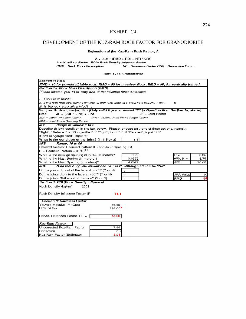
224
Estim ation of the K uz-R am Rock Factor, A
A = 0 .06 * (R M D + RDI + HF) * C(A)A = Kuz-Ram Factor RD I = Rock Density Influence FactorR M D = Rock M ass Description H F = Hardness Factor C(A) = Correction Factor
R ock T yp e: G ran od iorite
EXHIBIT C4
DEVELOPMENT OF THE KUZ-RAM ROCK FACTOR FOR GRANODIORITE
S ection 1: R M DR M D = 10 fo r p o w d ery /friab le ro c k ; R M D = 50 fo r m assiver R o ck ; R M D = JF, fo r vertica lly jo in te dS ection 1a: R o ck M ass D escrip tion (R M D )P le a se choose ye s (Y) to o n ly o ne of the following three questions:
i. Is this rock friable nii. Is this rock massive, with no jointing, or with joint spacing > blast hole spacing ? (y/n)iii. Is the rock vertically jointed? y
n
S ection 1b: Jo in t Factor, JF - (O n ly va lid i f yo u answ ered "Y " to Question i i i in S ection 1a, above)Note: JF = (JCF * JP S ) + JP A JF = Joint Factor JC F = Joint Condition Factor JPA = Vertical Joint Plane Angle Factor JPS = Joint P lane Spacing FactorJ C F R ange o f values: 1 to 2D escribe th jo in t cond ition in the box below. P lease, "Tight", "R e laxed" or "G ouge-filled": if "T ight", input "1 If jo in t is "gouge-filled", input "2"
choose on ly one of th ree options, "; if "R e laxed", input "1 .5";
nam ely:
W h a t is the con d ition of the jo in t? (1, 1.5 o r 2) 1 .5JP S R ange: 10 to 50Relevant facto rs: Reduced Patte rn (P) and Joint Spacing (S) P = Reduced Pattern = (B*S )05W hat is the average spac ing of jo in ts , in m eters? 0.25 p = 3.95W hat is the b last Burden (in m eters)? 3.6576 95% P = 3.75W hat is th e b last S pac ing (in m eters)? 4.2672 JPS 20.00JPA N ote that o n ly one answ er can b e "Yes", a lth o u g h a ll can be "No"Do th e jo in ts d ip out of th e face at >30o? (Y or N) yDo the jo in ts d ip in to th e face at >30o? (Y or N) n JP A Value 40Do th e jo in ts S tr ike out o f th e face? (Y or N) n RMD 65S ection 2 : RDI (R ock D ensity In fluence)R ock D ensity (kg //m 3) 2563
R ock D ensity Influence Facto r (F 14.1
S ection 3: H ardness F acto rY oung's M odulus, Y (Gpa)UCS (MPa)
66.85225.00
Hence, Hardness Factor, HF = 45.00
K uz-R am F ac to r |U ncorrected Kuz-R am Factor 7.44Correction 0.7Kuz-Ram Facto r (E stim ate) 5.21

APPENDIX D
CORE DIMENSIONS, SEISMIC VELOCITIES, AND DYNAMIC
YOUNG’S MODULI

CORE DIMENSIONS, SEISMIC VELOCITIES, AND DYNAMIC YOUNG’S MODULI
Uncorrected Corrected
Arriva l Times
Sample ID h (m) D (m) Vol (m3) Mass (g) p (kg/m3) S-wave (^s) P-wave (^s) S-wave (^s) P-wave (^s) Vs (m /s ) Vp (m /s ) E (Gpa)
WUSCM-K1 0.0999 0.0537 0.0002264 665.5 2939.334141 29.51 17.73 29.3045 17.5309 3 ,410 .40 5 ,700 .79 83.51
WUSCM-K2 0.1087 0.0540 0.0002486 725.4 2 ,917.45 31.32 18.18 31.1145 17.9809 3,493 .15 6 ,044 .61 88.95
WUSCM-K3 0.1095 0.0539 0.0002496 734.1 2,941.03 30.5 17.86 30.2945 17.6609 3,615 .67 6 ,202 .12 95.55
WUSCM-K4 0.1132 0.0546 0.0002655 758.0 2 ,854.94 33.3 19.9 33.0945 19.7009 3,421 .41 5 ,747 .45 81.92
Avg 0.1078 0.0540 0.0002475 720.8 2,913.2 3,485.16 5,923.74 87.48
Uncorrected Corrected
Arriva l Times
Sa mpl e ID h (m) D (m) Vol (m3) Mass (g) p (kg/m3) S-wave (^s) P-wave (^s) S-wave (^s) P-wave (^s) V s (m/s) Vp (m/s) E (Gpa)
WUSCM-L1 0.0588 0.0532 0.00013082 360.7 2 ,757.28 17.4 10.92 17.1945 10.7209 3,419.12 5 ,483.68 76.20
WUSCM-L2 0.0871 0.0536 0.00019635 546.0 2 ,780.78 24.6 15.9 24.3945 15.7009 3,568 .43 5 ,544 .27 81.19
WUSCM-L3 0.0875 0.0511 0.00017929 493.0 2 ,749.78 33.8 19.9 33.5945 19.7009 2,605.56 4 ,443.07 46.22
WUSCM-L4 0.0945 0.0537 0.00021404 594.9 2 ,779.45 26.6 16.42 26.3945 16.2209 3,580 .42 5 ,826 .02 85.27
WUSCM-L5 0.1052 0.0536 0.00023764 661.6 2 ,784.05 29.96 18.7 29.7545 18.5009 3,534.59 5 ,684.59 82.42
WUSCM-L6 0.1101 0.0520 0.00023363 645.0 2 ,760.75 - - - -
AVG 2,768.68 3,341.62 5,396.33 74.26
Uncorrected Corrected
Arriva l Times
Sa mpl e ID h (m) D (m) Vol (m3) Mass (g) p (kg/m3) S-wave (^s) P-wave (^s) S-wave (^s) P-wave (^s) Vs (m/s) Vp (m/s) E (Gpa)
WUSCM-M1 0.0323 0.0535 0.0000726 215.38 2 ,968.36 9.80 5.84 9.59 5.64 3 ,365 .99 5 ,725 .15 83.13
WUSCM-M2 0.0419 0.0534 0.0000937 266.74 2,845.63 13.48 8.28 13.27 8.08 3 ,154 .73 5 ,182 .28 68.29
WUSCM-M3 0.0652 0.0534 0.0001463 413.67 2 ,828.04 24.00 12.80 23.79 12.60 2 ,740 .34 5 ,174 .63 55.43
WUSCM-M4 0.1076 0.0534 0.0002412 702.90 2 ,914.70
WUSCM-M5 0.1089 0.0536 0.0002459 742.00 3,017 .32
Avg 2,914.81 3,087.02 5,360.69 68.95
Uncorrected Corrected
Arriva l Times
Sa mpl e ID h (m) D (m) Vol (m3) Mass (g) p (kg/m3) S-wave (^s) P-wave (^s) S-wave (^s) P-wave (^s) Vs (m/s) Vp (m/s) E (Gpa)
WUSCM-N1 0.0211 0.0313 0.0000162 43.48 2 ,678.48 7.6 4.6 7.3945 4.4009 2,846 .71 4 ,783.11 53.21
WUSCM-N2 0.0218 0.0314 0.0000169 46.31 2 ,745.30 7.4 3.6 7.1945 3.4009 3,025 .92 6 ,401 .25 68.18
WUSCM-N3- 0.0271 0.0314 0.0000211 55.24 2 ,624.15 12 6.2 11.7945 6.0009 2,298 .95 4 ,518.49 36.76
WUSCM-N4 0.0344 0.0314 0.0000267 71.5 2 ,682.35 14 9 13.7945 8.8009 2,493 .39 3 ,908 .12 38.58
WUSCM-N5 0.0440 0.0314 0.0000341 93.11 2730.106825 20.4 11.2 20.1945 11.0009 2,178 .81 3 ,999 .67 33.41
WUSCM-N3 0.0237 0.0314 0.0000184 49.66 2 ,699.87 16.2 11.6 15.9945 11.4009 1,482 .70 2 ,080 .10 11.68
WUSCM-N7 0.0359 0.0538 0.0000816 216.18 2 ,648.54 10.9 6.9 10.6945 6.7009 3,353 .59 5 ,352 .27 70.11
WUSCM-N6 0.0313 0.0536 0.0000706 12.7 8.2 12.4945 8.0009
Avg 2,686.97 2,525.72 4,434.72 44.56
226

APPENDIX E
PHOTO OF CORES USED IN ROCK CHARACTERIZATION

228
PHOTO OF CORES USED IN ROCK CHARACTERIZATION
Back row: Sembehun waste (limestone)
Middle row: Sembehun high-grade ore
Front row: Bom ore
Note: The initials of the host mine have been masked, in line with
that host’s request for anonymity

APPENDIX F
DENSITY DATA OBTAINED FROM W.U.S. COPPER’S GEOLOGY (ORE
CONTROL) SECTION, WITH THOSE ESTIMATED IN THIS
RESEARCH AT THE UNIVERSITY OF UTAH
(U OF U)

230DENSITY DATA OBTAINED FROM W.U.S. COPPER’S GEOLOGY (ORE
CONTROL) SECTION, WITH THOSE ESTIMATED IN THIS RESEARCH
AT THE UNIVERSITY OF UTAH (U OF U)
W.U.S. C opper values Estim ated (U o f U)
s.t ./ft3 s.t ./yd3 t/yd3 t/m 3 t/m 3
B om ore 0.1020 2.75 2.50 3.268 2.687
Sem behun High Grade 0.0909 2.45 2.23 2.912 2.915
Sem behun Low Grade 0.0850 2.30 2.08 2.723
lim e s to n e /d o lo m ite 0.0810 2.19 1.98 2.595 2.769
m onzon ite 0.0830 2.24 2.03 2.659
granod io rite 0.0800 2.16 1.96 2.563

APPENDIX G
A SUMMARY OF DATA OBTAINED FROM UNIAXIAL COMPRESSIVE
STRENGTH TESTING OF ROCKS FROM W.U.S. COPPER MINE

A SUMMARY OF DATA OBTAINED FROM UNIAXIAL COMPRESSIVE STRENGTH TESTING
OF ROCKS FROM W.U.S. COPPER MINE
SampleID
RockDescription D (m) A (m2)
mass(kg)
h (m)Density(kg/m3)
Kt (N/m) Kst (N/m) Ks (N/m) E (GPa) C0 (MPa)
K1East Side
Sembehun Waste
0 053 70 8 0 0 0 2 2 6 5 5 0 666 0 0999 2,939 3 1,108,429,643 3 6 5 4 8 4 2 8 4 6 1,59 0,918,6 09 0 0 18 178 6
K2 0 0539 7 0 0 0 0 2 2 8 7 7 0 725 0 108 7 2,917 4 1032,103,40 8 3 6 5 4 8 4 2 8 4 6 143 8,25 7,916 68 33 220 1
K3 0 053 865 0 0 0 2 2 7 8 8 0 734 0 1095 2,9 410 993353 ,415 3,65 4 8 4 2 8 4 6 1364 ,104843 05 57 096 2
K4 0 0 5 4 6 4 0 0 0 0 2 3 4 4 8 0 758 0 1132 2 8 5 4 9 964,993,986 3,65 4 8 4 2 8 4 6 1311,18 9,420 63 32 201 3
2 ,913 A v e ia g e 1,426,117,697 6 6 .8 5 19 9.1L2
West Side Sembehun
Waste (5220 Bench)
0 05359 0 0 0 2 2 5 5 6 00 546 0 0871 2,780 8 1,107,952,985 3,65 4 8 4 2 8 4 6 1 5 8 9 ,9 3 6 8 4 9 0136 091 1
L3 0 0510675 0 0 0 2 0 4 8 2 00 493 0 0875 2,749 8 830,036,163 3,65 4 8 4 2 8 4 6 1,073,932,510 45 90 065 7
L4 0 0537 0 0 0 2 2 6 4 8 0 595 0 0945 2,779 4 1,105,126,601 3 ,6 5 4 8 4 2 8 4 6 1,58 4,122,963 66 10 216 7
L5 0 0536375 0 0 0 2 2 5 9 6 00 662 0 1052 2,784 0 9 99316,958 3,65 4 8 4 2 8 4 6 1,375,375,948 04 02 242 6
L6 0 051975 0 0021217 00 645 0 1101 2,760 8 878,611,362 3,65 4 8 4 2 8 4 6 1,156,6710 01 60 03 00 3
5 9 .3 4 2 0 4.0 4M4 Sembehun
Ore (soft)0 0534 2 5 0 0022417 00 703 0 1076 2,914 7 829,637,254 3,654 8 4 2 8 4 6 1 0 7 3 ,2 6 4 8 2 4 5151 05 2
M5 0 0536 2 7 5 0 0 0 2 2 5 8 7 0 7 42 0 108 9 3,017 3 762,585,580 3,654 8 4 2 8 4 6 963,652,329 46 45 58 92,966 0 48 98 62 05
N1
Bom OreN2N3 27 15
N4 32 81
N5 26 312686.97 44 5 6 28.76
232

APPENDIX H
POINT LOAD DATA USED TO ESTIMATE UNIAXIAL COMPRESSIVE
STRENGTHS OF ROCKS
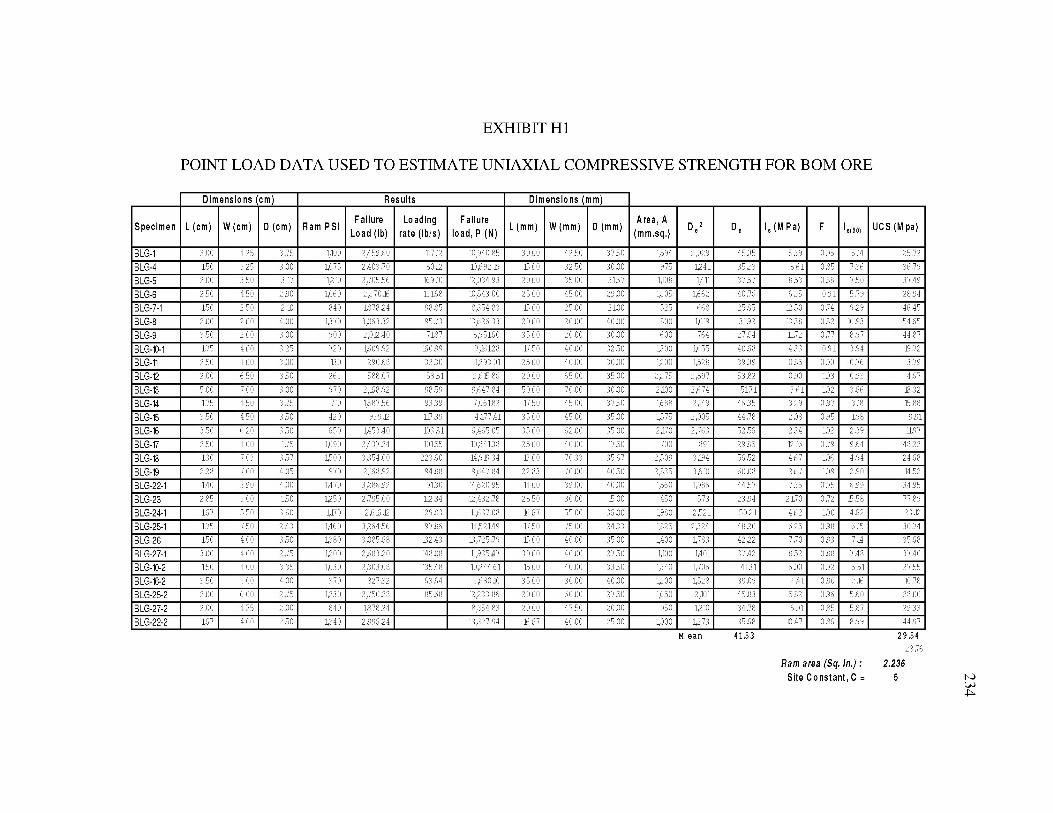
EXHIBIT H1
POINT LOAD DATA USED TO ESTIMATE UNIAXIAL COMPRESSIVE STRENGTH FOR BOM ORE
D im ens io n s (cm ) R e su lts D im ens io n s (mm)
Spec im en L (cm ) W (cm ) D (cm ) Ram P S IFa ilu re
Load (lb )
Load ing
rate (lb /s )
F a ilure
load , P (N )L (mm) W (mm) D (mm)
A re a , A
(m m .sq .) D e2 D e I s (M P a ) F I s(50) U C S (M pa)
BLG-1 3 00 4 25 43.75 4,100 2 ,4 5 9 6 0 11712 410,940.85 3 0 0 0 42 50 37 50 1594 2,029 4 5 0 5 5 39 0.95 45.14 25.72
BLG-4 150 3 2 5 43.00 1075 2 ,403.70 8012 410,692.19 1500 32 5 0 30 00 975 1241 35.23 8.61 0 .85 447.36 36.79
BLG-5 2 00 3 5 0 43.17 1210 2 ,7 0 5 5 6 16910 412,034.93 2 0 0 0 345 00 3167 1,108 1,411 37.57 8.53 0.88 447.50 37.49
BLG-6 2 5 0 4 5 0 2 9 0 4060 2 ,37016 13168 410,5 4 3 .00 2 5 0 0 445 00 29 00 1305 1662 4 0.76 6.35 4 9 1 445.79 28.94
BLG-7-1 150 2 5 0 42.10 840 1 8 7 8 2 4 98.85 48,354.83 1500 25 0 0 2100 4525 668 25.85 12.50 0.74 449.29 46.45
BLG-8 2 0 0 4 0 0 44.00 1370 3 ,0 6 3 3 2 95.73 413,626.33 2 0 0 0 20 0 0 40 00 800 1019 31.92 13.38 0.82 140.93 54 .65
BLG-9 3 5 0 2 0 0 43.00 900 2 ,012.40 7 1.87 48,951.60 35 00 20 0 0 30 00 600 7 64 2 7.64 11.72 0.77 448.97 44.87
BLG-10-1 1.75 4 0 0 43.25 720 1,609.92 160.99 47,161.28 17 50 40 0 0 32 50 1300 1,655 4 0.68 4.33 4 9 1 443.94 19.72
BLG-11 2 5 0 4 0 0 43.00 130 290.68 32.30 41,2 93.01 25 00 40 0 0 30 00 1200 1528 3 9.09 0 .85 4 90 440.76 3.79
BLG-12 2 0 0 6 5 0 43.50 263 5 88.07 58 .81 42,615.86 20 00 645 00 435 00 2 2 7 5 2,897 5 3 .82 0.90 403 440.93 4.67
BLG-13 5 0 0 74.00 43.00 97 0 2 ,168.92 9 8.59 49,6 47.84 50 00 70 0 0 30 00 2,100 2,674 51.71 4 6 1 402 443.66 18.32
BLG-14 1.75 44.50 43.75 710 1,58 7.56 93.39 47,061.82 17 50 445 00 37 50 1688 2,149 4 6.35 3.29 0.97 43.18 15.88
BLG-15 3 5 0 4 5 0 3 5 0 420 93912 11739 4 ,177.41 35 00 45 0 0 35 00 4575 2,005 4 4.78 2 0 8 0 9 5 198 9 9 1
BLG-16 3 5 0 46.20 43.50 650 1,453.40 103.81 46,465.05 35 00 62 0 0 435 00 4,170 2,763 52 .56 2.34 402 2 3 9 11.97
BLG-17 2 5 0 44.00 41.75 4090 2 ,4 3 7 2 4 101.55 140,841.38 25 00 40 0 0 417 50 700 891 29.85 12.16 4 .79 9.64 48.22
BLG-18 130 74.03 43.57 4500 3 3 5 4 .0 0 223.60 414,919.34 13 00 70 33 435 67 2 5 0 9 3,194 56 .52 4 67 406 4.94 24.68
BLG-19 2 2 8 74.00 44.05 97 0 2 ,16892 9 4.88 49,6 47.84 22 83 40 0 0 40 50 2 8 3 5 3 610 6 0.08 4 67 409 2.90 14.52
BLG-22-1 1.40 3 9 0 44.00 1470 3 2 8 6 9 2 91.30 414,6 20.95 14 00 39 0 0 40 00 1560 1986 4 4.57 7.36 0 .95 6.99 34.95
BLG-23 2 85 34.00 41.50 1250 2 ,7 9 5 0 0 112.34 412,432.78 28 50 30 0 0 415 00 450 573 23.94 21.70 0.72 15.58 77.89
BLG-24-1 167 45.50 43.60 1170 2,61612 129.83 141,6 37.08 16 67 455 00 36 00 4980 2 5 2 1 5 0 .2 1 4 62 400 4.62 23.12
BLG-25-1 1.75 47.50 42.43 4460 3 2 6 4 5 6 97.86 414,521.49 17 50 745 00 24 33 1825 2,324 4 8.20 6 .25 0.98 6.15 30.74
BLG-26 150 44.00 43.50 1380 3 ,0 8 5 6 8 132.43 143,725.79 15 00 40 00 435 00 4400 1783 42.22 7.70 4 9 3 7.14 35.68
BLG-27-1 3 0 0 44.00 42.75 4200 2 6 8 3 2 0 148.08 141,935.47 30 00 40 00 27 50 1,100 1,401 37.42 4 52 440.88 7.48 37.40
BLG-10-2 150 44.00 43.35 4030 2 3 0 3 .0 8 135.48 140,244.61 15 00 40 00 33 50 4340 1706 4 1.31 6.00 440.92 5.51 27.55
BLG-16-2 3 5 0 34.00 44.00 370 8 2 7 3 2 6 3.64 43,680.10 35 00 40 00 40 00 4200 1528 3 9.09 2.41 440.90 2.16 10.78
BLG-25-2 2 0 0 46.00 42.75 1230 2 ,7 5 0 2 8 4 5 6 8 412,233.86 20 00 40 00 27 50 1,650 2,101 4 5 8 3 5.82 44 .96 5 .60 28.00
BLG-27-2 2 0 0 44.75 42.00 840 1 8 7 8 2 4 48,354.83 20 00 47 50 20 00 950 1210 3 4.78 6.91 440.85 5 .87 29.33
BLG-22-2 167 44.00 42.50 1340 2 ,9 9 6 2 4 413,327.94 16 67 40 00 425 00 4000 1273 3 5 .68 10.47 44 .86 8.99 44.97M ean 41.53 29.54
28 .76
R am area (Sq. I n . ) : 2.236 S ite C o n s ta n t , C = 5
234

EXHIBIT H2
POINT LOAD DATA USED TO ESTIMATE UNIAXIAL COMPRESSIVE STRENGTH
FOR SEMBEHUN HIGH-GRADE ORE
D i m e n s i o n s ( c m ) R e s u l t s D i m e n s i o n s ( m m )
S p e c i m e n L ( c m ) D ( c m ) W ( c m ) R a m P S IF a i l u r e
L o a d ( l b)F a i l u r e
l o a d , P ( N )L ( m m ) W ( m m ) D ( m m )
A r e a , A ( m m . s q . ) D e 2 D e Is ( M P a ) F I s(50) U C S ( M p a )
SRW-2 2 0 0 4 .00 4 3 0 4 30 1 4 0 8 6 8 6 2 6 6 1 2 20.00 4 3 0 0 40.00 4720 2,190 46 .80 4 8 6 0.97 2.78 138.86
SRW-1 2 .77 3 5 0 4 2 0 430 961.48 4 2 7 6 8 8 27.67 4 2 0 0 35 .00 4470 1872 43.26 4 2 9 0.94 2.14 4 0705
SRW-5 2 0 0 3 5 0 6 10 1 0 2 23.60 4 9 4 6 2 20.00 4 1.00 35 .00 2 ,135 2,718 52.14 0.37 402 0.37 18.64
SRW-6 2 5 0 4 .00 4 0 0 4 45 5 47.82 2 , 4 3 6 8 2 25.00 4 0 0 0 40.00 4600 2 0 3 7 45.14 1.20 0.95 1.14 57.12
SRW-7 2 5 0 3 8 0 4 .40 80 47 888 795.70 25.00 4 4 0 0 38 .00 4672 2,129 46.14 0.37 0.96 0.36 18.02
SRW-10 2 17 2 .47 4 0 0 3 40 7 60.24 3381 .72 21.67 4 0 0 0 24.67 4480 1884 43.41 1.79 0.94 1.68 84.20
SRW-4 2 13 4 .00 4 2 5 440 4 6 0 2 4 3381 .72 2133 4 2 5 0 4 0 0 0 4700 2,165 4 6 5 2 156 0 9 7 151 7 5 6 3
SRW-8 4 5 0 3 6 0 5 5 0 5 0 11180 4 9 7 3 1 45.00 5 5 0 0 36 .00 4980 2,521 5 0 . 2 1 0.20 400 0.20 4 88
SRW-11 2 0 0 3 7 0 5 5 0 2 00 447.20 1,9 89 .2 4 20.00 4 5 0 0 37 .00 2 ,035 2,591 5 0 . 9 0 0.77 401 0.77 38 .70
SRW-9 177 4 2 0 4 74 5 5 160 3 57 .76 1,591.40 17.67 4 5 5 0 42.00 4,171 4 0 3 7 63 .54 4 3 9 411 0.44 21.95
SRW-3 2 0 0 3 7 5 4 0 0 480 1 0 7 3 2 8 4 ,774.19 20.00 4 0 0 0 37 .50 4,250 2,865 53 .5 2 467 403 1.72 85.92
SRW-12 150 3 5 0 4 54 5 0 4 00 894.40 3 ,9 78 .4 9 15.00 5 5 0 0 35 .00 4925 2,451 49.51 462 1.00 1.62 80.80
SRW-13 3 5 7 3 .00 4 0 0 130 290.68 1,293.01 35 .67 5 0 0 0 30 .00 4500 1,910 43.70 4 6 8 4 94 0.64 31.86
SRW-14 2 5 7 3 7 5 4 0 0 3 40 7 6 0 2 4 3 ,381.72 25.67 8 0 0 0 37 .50 3,000 3 8 2 0 61.80 0.89 410 0.97 48.70
SRW-15 2 .40 3 7 5 4 7 5 3 00 6 7 0 8 0 2 ,9 83 .87 24.00 4 7 5 0 37 .50 1781 2 2 6 8 47.62 1.32 0.98 1.29 64.36
SRW-16 2 9 3 4 7 0 4 9 0 6 60 1475.76 6 ,5 64 .5 1 29.33 5 9 0 0 47.00 2,773 3,531 5 9 . 4 2 486 1.08 2.01 400.47
M e a n 5 0 . 2 3 6 1 3 862 .05
R am area (Sq. I n . ) : 2 .236 S i t e C o n s t a n t , C = 50
235

EXHIBIT H3
POINT LOAD DATA USED TO ESTIMATE UNIAXIAL COMPRESSIVE STRENGTH
FOR SEMBEHUN LOW-GRADE ORE
Dimensions cm) Results Dimensions (mm)
Specimen L (cm) D (cm) W (cm) Ram PSIFailure
Load (lb)Failure
load, P (N)L (mm) W (mm) D (mm)
Area, A (mm.sq.) D e2 D e Is (MPa) F Is(50) UCS (M pa)
S R F-19 2 50 3 3 5 4 5 0 4,040 2 3 2 5 .4 4 4 0 3 4 4 0 7 2 5 0 0 4 5.00 33 50 4508 4 41,919 43 81 5.39 4 9 4 5 0 8 253 90
S R F-12 2 0 0 2 80 5 0 0 485 4084.46 4,823 92 2 0 0 0 40 00 28 00 1400 1783 42 22 2.71 0 93 4 51 425 39
S R F-14 180 2 3 7 3 0 0 430 961.48 4 2 7 6 8 8 1800 4 0 0 0 2 3 6 7 710 404 30 07 4 .73 4 8 0 3.76 438 16
S R F-10 2.75 2 2 7 4 25 4 20 0 2 ,6 8 3 2 0 11935.47 2 7 5 0 42 50 2 2 6 7 963 1227 3 5 0 2 4 .73 0 8 5 8 2 9 414 52
S R F -5 190 4.40 4.75 1285 2 8 7 3 2 6 12 ,78090 1900 4 7 5 0 4 4 0 0 4 ,090 2,661 51.59 4 80 401 4.87 243 54
S R F-13 2 0 0 3 2 0 3.75 500 1118 00 4,97311 2 0 0 0 3 7 5 0 32 00 4200 1528 39 09 3 2 5 0 9 0 4 9 1 445 68
S R F-16 2 50 2 50 4 5 0 650 1453.40 6 ,4 6 5 0 5 2 5 0 0 45.00 25 00 1125 1432 3 7 8 5 4 5 1 0 8 8 4 98 199 09
SRF-11 183 3 50 3 3 5 520 4162.72 5,172 04 18 33 43 50 35 00 4173 1493 38 64 3.46 0 8 9 3 0 9 45 4 2 5
S R F -9 210 2.70 4 50 360 8 0 4 9 6 3 5 8 0 6 4 2100 45.00 27 00 4,215 1547 39 33 4 3 1 0 9 0 4 08 103 88
S R F-18 1.75 3 2 0 4 8 5 700 4,56520 6,962 36 1750 48 50 32 00 1552 1976 44.45 4 52 0 9 5 44 34 34 467 09
S R F -2 157 3 93 4 .75 1100 2 ,4 5 9 6 0 10 ,94085 1567 4 7 5 0 39 33 2,655 3 3 8 0 5814 3 2 4 107 4 .46 173 19
S R F -2 0 2 0 0 3 0 0 4 00 900 2,012.40 8,95160 2 0 0 0 40.00 30 00 2,400 3,056 5 5 2 8 2 93 105 3 06 453 24
S R F -4 130 3 0 0 4 00 450 1006 20 4 ,4 7 5 8 0 1300 50.00 30 00 4,500 1910 43.70 2 3 4 4 9 4 2 21 410 29
S R F-15 180 3 50 4 50 770 1721.72 7,658 59 1800 45.00 35 00 4575 2,005 44.78 3 82 0 9 5 3 63 481 .71
S R F -7 315 2 50 3 60 1040 2 3 2 5 .4 4 1 0 3 4 4 0 7 3150 4 6 0 0 25 00 900 1146 33 85 4 03 4 8 4 4 57 478 69
M san 4252 M san 199 51
fiam area {Sq.&.} : 2236Sits Constant, C = 50
236

APPENDIX I
CRUSHING CIRCUIT CHARACTERISTICS

238
CRUSHING CIRCUIT CHARACTERISTICS
Feature ValueCRUSHERSTypes Jaw (x1) Cone (x2)Feed rate through circuit 220(st/h) (200 t/h)Hours of operation (per day) 12
Jaw Crusher SettingsGape 1117.6 mm x 787.4 mm
(44 in. x 31 in.)Open Side Setting (OSS) 177.8 mm (7 in.)Closed Side Setting (CSS) 101.6 mm (4 in.)
Cone 1 SettingsGape 161.925 mm (6.375 in.)Open Side Setting (OSS) 127 mm (5 in.)Closed Side Setting (CSS) 12.7 mm (0.5 in.)
Cone 2 SettingsGape 73.025 mm (2.875 in.)Open Side Setting (OSS) 44.45 mm (1.75 in.)Closed Side Setting (CSS) 6.35 mm (0.25 in.)
SCREENSNo. of Screens 2Screen 1Dimensions of screen 6.096 m x 2.1336 m (20 ft x 7 ft )No. of decks 3No. of screen panels per deck 5Dimensions of panel 1.2192 x 2.1336 m (4 ft x 7 ft )Screen size on Deck 1 31.75 mm (1.25 inches)Screen size on Deck 2 28.575 mm (1.125 inches) (x1); 9.525
mm (0.375 inches) (x4)Screen size on Deck 3 6.35 mm (0.25 inches)Inclination of screen Horizontal
Screen 2Dimensions of screen 6.096 m x 2.1336 m (20 ft x 7 ft )No. of decks 3No. of screen panels per deck 5Dimensions of panel 1.2192 x 2.1336 m (4 ft x 7 ft )Screen size on Deck 1 15.875 mm (0.625 inches)Screen size on Deck 2 12.7 mm (0.5 inches)Screen size on Deck 3 6.35 mm (0.25 inches)Inclination of screen Horizontal

REFERENCES
Ash, R.L. 1963. The mechanics of rock blasting (Part 1). In Pit and Quarry 56(2): 98100.
Bedair, A 1996. Digital Image Analysis of Rock Fragmentation from Blasting, Ph.D. thesis, Department of Mining and Metallurgical Engineering, McGill University, Montreal.
Bergmann, O.R., Riggle, J.W. and Wu, F.C. 1973. Model rock blasting - Effect of explosives properties and other variables on blasting results. In Int. J. Rock Mechanics & Mining Sciences, vol 10, pp 585-612.
Bergstrom, B.H. 1985. Crushability and grindability. In SME Mineral Processing Handbook, Ed: N.L. Weiss, New York, vol. 2, in Section 30 "Sampling and Testing", pp 65-68.
Bhattacharyya, A. 2014. Dependence of rates of breakage on fines content in wet ball mill grinding, M.S. thesis, Department of Metallurgical Engineering, University of Utah
BoBo, T. n.d. What’s new with the digital image analysis software Split-Desktop, Split Engineering. Split Engineering, LLC, 110 S. Church St., Tucson, Arizona, USA
Bond, F.C. 1952. The Third Theory of Comminution. In Trans. A.I.M .E, v. 193, pp. 484-494.
Brandt, D., Martinez, I., French, T., Slattery, L., Baker, G. 2011. Better fragmentation through team work at Dos Pobres Mine, Safford, Arizona. SME, November 2011
Csoke B, Petho S, Foldesi J and Meszaros, L. 1996. Optimization of stone-quarry technologies. In Intl. Jnl. o f Mineral Processing 44-45. 447 - 459.
Chung, S.H. and Katsabanis, P.D. 2000. Fragmentation prediction using improved engineering formulas. In Int J. Fragmentation by blasting, vol 4, pp 198-207.
Cunningham, C.V.B. 1983. The Kuz—Ram model for prediction of fragmentation from blasting. In Proceedings o f the first international symposium on rock fragmentation by blasting, Lulea, Sweden. p. 439-54.

240Cunningham, C.V.B. 1987. Fragmentation estimations and the Kuz—Ram model - Four years on. In Proceedings o f the second international symposium on rock fragmentation by blasting, Keystone, Colorado. p. 475-87.
Cunningham, C.V.B. 2005. The Kuz-Ram fragmentation model - 20 years on. In Brighton Conference proceedings. Ed. R. Holmberg et al.
Dance, A., Valery W., Jankovic, A., La Rosa, D., and Esen, S. 2007. Maintaining the benefit - how to ensure Mine to Mill continues to work fo r you. , Ninth Mill Operators Conference, Fremantle, WA, 19 to 21 March, 2007, pg. 1-8 (see pg 3)
Edgar, J and Pfleider, E.P. 1972. Mining and Milling, an Interrelated Fragmentation System. In Society o f Mining Engineers, AIME, Transactions Vol 252, March 1972. Page 46 - 49
Eloranta, J. 2014. Non-ideal blasting for ideal grinding - Part Two. In The Journal o f Explosives Engineering. Volume 31 Number 5, September/October 2014. Pg 26- 31.
Eloranta, J., Palangio, T., Palangio, T.C. and Workman L. 2007. Size matters on the Mesabi Range. In International Society o f Explosive Engineers, 2007G Volume 1.
Floyd, J. n.d. Efficient Blasting Techniques
Hall, J. and Brunton, I. 2001. Critical Comparison of Julius Kruttschnitt Mineral Research Centre (JKMRC) Blast Fragmentation Models. In EXPLO 2001, Hunter Valley, NSW, 28 - 31 October 2001. Pages 207 - 212.
Herbst, J.A. 1971. Batch Ball Mill Simulation: An Approach fo r Wet Systems. D. Eng. Dissertation, University of California, Berkeley, California.
Herbst, J.A. and Fuerstenau, D.W. 1968. The zero order production of fine sizes in comminution and its implications in simulation. In Transactions o f SME, AIME, December 1968, vol. 241. Pages 538 - 548
Herbst, J.A., Grandy, G.A., and Mika, T.S. 1968. On the development and use o f lumped parameter models fo r open- and closed-circuit grinding. Trans. Inst. Min. Met. Section C, 77, pp. 193-198, (1968).
Herbst, J.A., Grandy, G.A. and Fuerstenau, D.W. 1973. Population Balance Models fo r the Design o f Continuous Grinding Mills. Paper 19 of International Mineral Processing Congress, London(1973).
Herbst, J.A., Rajamani, K. and Kinneberg, D.J. 1977. ESTIMILL: A program fo r grinding simulation and parameter estimation with linear models.
Herbst, J.A., Siddique, M., Rajamani, K. and Sanchez, E. 1983. Population Balance Approach to Ball Mill Scale-Up: Bench and Pilot Scale Investigations. In SME o f AIME Transactions Vol 272. Pp 1945 - 1954.

241Himmelblau, D.M., and Bischoff, K.B. 1968. Process analysis and simulation: Deterministic systems. J. Wiley, New York, 1968.
Hustrulid, W. 1999. Blasting Principles fo r Open Pit Mining, Vol. 1: General Design Concepts. CRC Press, Taylor & Francis Group, Boca Raton, London, New York
Infomine USA Inc. Costmine Division 2013. Mine and Mill Equipment Costs - An Estimator’s Guide
Jankovic, A; Valery, W.; Davis, E., 2004. Cement Grinding Optimisation. In Minerals Engineering, vol 17 (2004), pp. 1075-1081.
Julius Kruttschnitt Mineral Research Center (JKMRC) 2012. Mine to Mill Process Optimization (Course notes for short course on Mine-to-mill process optimization at SME conference 2012). JK Tech SMI Technology Transfer
Kanchibotla, S.S., 2001. Optimum Blasting? Is it Minimum Cost Per Broken Rock or Maximum Value Per Broken Rock? In EXPLO 2001 Hunter Valley, NSW, 28 - 31 October; pages 35 - 40.
Kanchibotla, S.S., Valery, W. and Morrell, S. 1999. Modelling Fines in Blast Fragmentation and its Impact on Crushing and Grinding. In Explo ’99, Kalgoorlie, WA, November 7 - 11. pp 137 - 144.
Kemeny, J.M., Devgan A., Hagaman, R.M., Wu, X. 1993. Analysis o f rock fragmentation using digital image processing
Kemeny, J.M., Mofya, E., Kaunda, R., and Lever, P. 2001. Improvements in Blast Fragmentation Models Using Digital Image Processing. EXPLO 2001, Hunter Valley, NSW, 28 - 31 October 2001
Kick, F. 1885. Das Gesetz der proportionalen Widerstande und seine anwendung.(The law o f proportional resistance and its application) Leipzig, Germany.
Kim, J.H. 1974. A Normalized Model fo r Wet Batch Ball Milling. Ph.D. Dissertation, University of Utah, Salt Lake City, Utah.
King, R.P. 2012. Modeling and simulation o f mineral processing systems. Second Edition. Ed. Schneider, CL and King, E.A. Society for Mining, Metallurgy and Exploration, Englewood, Colorado.
Konya, C. J. 1968. Spacing o f Explosive Charges. MS Thesis, Department of Mining and Petroleum Engineering, University of Missouri at Rolla
Kou, S. and Rustan, A. 1993. Computerized design and result prediction of bench blasting. In Proc 4th Int Symp on Rock Fragmentation by Blasting, H-P Rossmanith ed, pp 263-271. Balkema, Rotterdam.
Kuznetsov, V.M. 1973. The mean diameter of fragments formed by blasting rock. In Sov Min Sci; 9:144-8.

242Langefors, U., & Kihlstrom, B. 1963. The modern technique o f rock blasting. Almqvist & Wicksell, Uppsala, Sweden
Larsson, B. 1974. Report on blasting of high and low benches - fragmentation from production blasts. In Proc Discussion meeting BK 74, pp 247 - 273. Swedish Rock Construction Committee, Stockholm
Latchireddi, S.R. 2013. Grate discharge vs overflow ball mills for fine grinding. M.S Thesis, University of Utah
Levenspiel, O., and Bischoff, K.B. 1963. Patterns of flow in chemical process vessels. In Advances in Chemical Engineering, edit. T.B. Drew, et. Al, Academic Press, New York, p p .95-198, 1963.
Lilly, P.A. 1986. An empirical method o f assessing rock mass blastability. The AuslMM/IE Aust Newman Combined Group, Large Open Pit Mining Conference October 1986. Pages 89 - 92.
Luz, J. A. M., Milhomem, F. O. 2013. Scale-up o f Crushing Tests. Twenty-third International Mining Congress & Exhibition of Turkey, 16-19 April.
Lynch, A.J. and Morrison, R.D. 1999. Simulation in mineral processing history, present status and possibilities. In The Journal o f the South African Institutte o f Mining and Metallurgy. October-December. pp 283 - 288
Malghan, S.G., Fuerstenau, D.W, 1976. The Scale-up of Ball Mills Using Population Balance Models and Specific Power Input. In Symposium Zerkleinern, Dechma- Monographien, Vol. 79, Part II No. 1586, p. 613.
McCarter, M.K. 2014. Unpublished, class notes on surface mining - University of Utah
MacKenzie, A.S. 1966. The Cost of Explosives, do you evaluate it properly? In Mining Congress Journal, Vol. 52 Issue 5. Pages 32 - 41.
MacKenzie, A.S. 1967. Optimum Blasting; 28th Annual Mining Symposium and the Fortieth Annual Meeting of the Minnesota Section, AIME.
Maerz, N. H., 1998. Aggregate sizing and shape determination using digital image processing. Center for Aggregates Research (ICAR) Sixth Annual Symposium Proceedings, St. Louis, Missouri, April 19-20, pp. 195-203.
Maerz, N.H., Palangio, T.C., Palangio, T.W., Elsey, K. 2007. Optical sizing analysis of blasted rock: lessons learned. In European Federation o f Explosives Engineers
Maerz, N.H., Zhou, W. 1998. Optical digital fragmentation measuring systems - inherent sources of error. In FRAGBLAST, the International Journal fo r Blasting and Fragmentation, Vol. 2, No. 4, pp. 415 - 431.
Magdalinovic, N. 1989. A Procedure for Rapid Determination of the Bond Work Index. In International Journal o f Mineral Processing, 25, 41-46.

243Magdalinovic, N., 1990. Mathematical Model for Determination of an Optimal Crusher Product size. In Aufbereitungs-Technik 31, Nr 5
Magdalinovic, N., Magdalinovic, S., Jovanovic, R. and Stanujkic, D. 2011. Is there a material constant which characterises mineral resources grindability? In Annual o f the university o f mining and geology “st. Ivan rilski”, Vol. 54, Part II.
Mika, T.S. 1970. Population balance models o f a continuous grinding mill as a distributed process. Doctor of Engineering dissertation, University of California, Berkeley, December 1970.
Mika, T.S., Berlioz, L.M. and Fuerstenau, D.W. 1967. An Approach to the Kinetics of Dry Batch Ball Milling”. In Zerkleinern, 2nd European Symposium on Comminution. Edit. Rumpf, H. and Pietsch, W. Amsterdam Dechema-Monographien, 57, Part I, pp. 205 - 240.
Moser, P. 2003. Less fines production in aggregate and industrial minerals industry. In Proc EFEE 2nd World Conf on Explo & Blasting. R Holmberg ed, pp 335-343. Balkema, Rotterdam.
Montgomery, D.C. and Runger G.C. 2011. Applied Statistics and Probability fo r Engineers. Wiley & Sons, Inc.
Mular, A.L. 1989. Modelling, simulation and optimization of mineral processing circuits. In Challenges in Mineral Processing, ed. K.V.S Sastry and M.C. Fuerstenau, SME, Inc., Littleton, 323
Mwansa, S., Dance, A., Annandale, D., Kok, D., and Bisiaux B. 2010. Integration and Optimisation o f Blasting, Crushing and Grinding at the Newmont Ahafo Operation
Nematollahi, H 1994. New size laboratory ball mill fo r Bond Work Index determination. SME non-meeting paper 93-315, 1993
Nielsen, K. and Kristiansen, J. 1996. Blasting-crushing-grinding: Optimization of an integrated comminution system. In Proc 5th Int Symp on Rock Fragmentation by Blasting, B Mohanty ed, pp 269-277. Balkema, Rotterdam.
Ouchterlony, F 2003. Influence of blasting on the size distribution and properties of muckpile fragments, a state-of-the-art review. In MinFo project P2000-10: Energioptimering vid nedbrytning/Energy optimization in comminution. Lulea University of Technology.
©Ouchterlony, F. 2005. The Swebrec function: linking fragmentation by blasting and crushing. In Mining Technology (Trans. Inst. Min. Metall. A) February 2005.
Palangio, T.W., Palangio T.C., Maerz, N 2005. Advanced automatic optical blast fragmentation sizing and tracking. In Brighton Conference Proceedings, R. Holmberg et al.

244Preece, D.S., and Chung, S.H. 2003. Blasting induced rock fragmentation prediction using the RHT constitutive model fo r brittle materials.
Preece, D.S., Jensen R.P., and Chung S.H. 2001. Development and Application o f a 3-D Rock Blast Computer Modeling Capability Using Discrete Elements - DMCBLAST_3D*
Preece, D.S., and Lownds, C.M. 2008. 3D computer simulation o f bench blasting with precise delay timing
Rajamani, R.K. 2012. Course notes (unpublished), MetE 7910, Department of Metallurgical Engineering, University of Utah, Fall 2012.
Rittinger, R.P. 1867. Lehrbuch der Aufbereitungskunde (Textbook o f the Processing Art). Ernst and Korn, Berlin, Germany.
Rogers, W., Kanchibotla, S.S., Tordoir, A., Ako, S., Engmann, E., and Bisiaux, B. 2012a. Solutions To Reduce Blast-Induced Ore Loss & Dilution A t Ahafo Gold Mine In Ghana. SME Annual Meeting Feb. 19 - 22, 2012, Seattle, WA
Rogers, W., Kanchibotla, S.S., Tordoir, A., Ako, S., Engmann, E., and Bisiaux, B. 2012b. Understanding blast movement and its impacts on grade control at Ahafo Gold Mine in Ghana. International Society of Explosives Engineers. Nashville, Tennessee.
Rosin P, Rammler E. 1933. The laws governing the fineness of powdered coal. In J. Inst Fuel 1933;7:29- 36.
Rowland, C.A. Jr, and McIvor, R.E. 2009. The Bond Standard for Comminution Efficiency. In Recent Advances in Mineral Processing Plant Design, SME, 2009
Rustan, A. 1981. Fragmentation influencing factors in rock blasting. In Teknisk rapport 1981: 38T, Lulea University of Technology, Lulea, Sweden. In Swedish.
Sastry, K.V.S. and Lofftus, K.D. 1989. Challenges and opportunities in modeling and simulation of mineral processing systems. In Challenges in Mineral Processing, ed. K.V.S. Sastry and M.C. Fuerstenau, SME, Inc., Littleton, 369
Sastry, K.V.S. 1990. Principles and methodology of mineral processing modeling. In Control '90 - Mineral and Metallurgical Processing, ed. R.K. Rajamani and J.A. Herbst, SME Inc., Littleton, Colorado.
Scaw Metals Group n.d. Media Charge Strings Spreadsheet. In Molycop Tools V.2.0
Schuhmann R. 1940. Technical publication 1189. New York (NY). American Institute of Mining and Metallurgical Engineers; 1940.
Siddique, M. 1977. A kinetic approach to ball mill scale-up fo r dry and wet systems. MS thesis, Department of Mining, Metallurgical and Fuels Engineering, University of Utah
Singh, S.P. and Narendrula, R. 2005. Characteristics of the blasted muck and the loader’s productivity. In International Society o f Explosives Engineers 2005G Volume 2.

245Tavares, L.M. and Carvalho, R.M. 2007. Impact work index prediction from continuum damage model of particle fracture. In Minerals Engineering, Elsevier. Vol. 20 pp1368- 1375
Thomas, S., Rafiei, S., Maghsoodlou, S. and Afzali, A. 2014. Foundations o f Nanotechnology. Volume 2: Nanoelements Formation and interaction. AAP Research notes on Nanoscience and Nanotechnology.
Thornton, D., Sprott, D., and Brunton, I. 2005. Measuring blast movement to reduce ore loss and dilution. In International Society o f Explosives Engineers
Tucker, S.A. 2001. Optimal open p it planning and design. MSc thesis, Department of Mining Engineering, Kwame Nkrumah University of Science and Technology, School of Mines, Tarkwa, Ghana.
U.S. Army Corps of Engineers 2009. Appendix L - Guide for Estimating Drill Steel and Drill Bit Costs In Construction Equipment Ownership and Operating Expense Schedule Region III. EP 1110-1-8 Volume 3.
Utley, R. W. 2002. Selection and Sizing of Primary Crushers. In Mineral Processing Plant Design, Practice, and Control: Proceedings - Volume 1. Mular A. L.; Halbe, D. N.; Barratt D. J. (ed.), SME, Littleton, Colorado, pp. 584 - 605.
Valery, W and Jankovic, A 2002. The future o f comminution. JKMRC, University of Queensland, Brisbane, Australia; 34th IOC on Mining and Metallurgy, 30 Sept.-3 Oct., Hotel Jezero, Bor Lake, Yugoslavia
Valery Jnr., W., La Rosa, D., Jankovic, A. 2004. Mining and Milling Process Integration and Optimisation. Presented at the SME 2004 Conference, Denver, CO. 23-25 February.
Vermeulen, L. A., Howat, D.D., and Gough, C. L.M., 1983. Theories of ball wear and the results of a marked-ball test in ball milling. In Journal o f Southern African Institute o f Mining and Metallurgy.
Whiten, W.J. 1973. The simulation of crushing plants with models developed using multiple spline regression. In Application o f computer methods in the Mineral industry Eds MDG Salamon and Lancaster. S. Afr. Inst. Min. Metall. Johannesburg, 1973. P317- 323
Whiten, W.J., Walter, G.W. and White, M.E. 1973. A breakage function suitable fo r crusher models. 4TH Tewksbury Symposium, Melbourne, Feb. P19.1-19.32
Widzyk-Capehart, E. and Lilly. P. 2001. A Review of General Considerations for Assessing Rock Mass Blastability and Fragmentation. In Explo 2001, Hunter Valley, NSW, October 28-31.
Wills, B. 2006. Wills’ Mineral Processing Technology; Seventh Edition, Copyright 2006, ed. Napier-Munn

246Workman, L. and Eloranta, J. 2003. The effects of Blasting on Crushing and Grinding Efficiency and Energy Consumption. In Proceedings o f 2 9 th Conference on Explosives and Blasting Technique, Nashville, TN, 2003