Lechner 1

An Evaluation of Public-Sector-Sponsored Continuous Vocational

Training Programs in East Germany

Michael Lechner∗

Abstract

This study analyses the effects of public-sector-sponsored continuous vocational training and

retraining in East Germany after unification with West Germany in 1990. It presents

econometric estimates of the average gains from training participation in terms of

employment probabilities, earnings, and career prospects after the completion of training

using a matching approach. The data is from the German Socio-Economic Panel (GSOEP,

1990-1996). The GSOEP allows the researcher to observe individual behavior on a monthly

or on a yearly basis. The results suggest that despite large public expenditures there are no

positive effects in the first years after training.

∗ Michael Lechner, Professor of Econometrics, University of St. Gallen, Swiss Institute for International

Economics and Applied Economic Research (SIAW), Dufourstr. 48, CH-9000 St. Gallen, Switzerland,

Michael.Lechner@unisg.ch, http://www.siaw.unisg.ch/lechner

Financial support from the Deutsche Forschungsgemeinschaft and the Swiss National Science Foundation is

gratefully acknowledged. I thank the DIW for supplying the data of the GSOEP. Furthermore, I thank Achim

Fox and Klaus Kornmesser for competent help with the data. I also thank Martin Eichler and participants of

seminars at the Universities of Berlin (Humboldt), Frankfurt (Oder), Heidelberg, Hohenheim, Jena, Magdeburg,

München, and St. Gallen, at the CENTER in Tilburg, and at the Tinbergen Institute in Amsterdam, as well as

participants of the 6th Conference on Panel Data in Amsterdam and the annual conference of the 'Verein für

Socialpolitik', for helpful comments and suggestions on an earlier version of this paper. Discussions with Bernd

Fitzenberger and Hedwig Prey, as well as the comments of two anonymous referees, were also very valuable for

revising this work. All remaining errors are my own.

published in The Journal of Human Resources, 35, 347-375, 2000

Lechner 2

I. Introduction

Unification of the East and West German economies in July 1990 - the Economic, Monetary,

and Social Union - came as a shock to the formerly centrally planned East German economy.

The almost immediate imposition of the West German type of market economy with all its

distinctive institutional features and its relative prices led to dramatic imbalances in particular

in the East German labor markets. For example the official unemployment rate rose from

about 2 percent in the German Democratic Republic (GDR) to more than 15 percent in 1992.

It remained on that level for the following years. To avoid higher unemployment as well as to

adjust the stock of human capital to the new labor demand structure the government

conducted active labor market policies on a large scale. The focus of this paper is on the

effects of the continuous vocational training and retraining part of these policies for workers

of the former GDR participating in schemes that began after July 1990 and before April

1993.1

The paper contributes to the ongoing discussion of the effectiveness of public-sector-

sponsored training in East Germany by analyzing the participation decision before obtaining

microeconometric evaluation results for several variables measuring the actual and

prospective individual position in the labor markets. The findings suggest that in the short run

public-sector-sponsored training has a negative impact, because it reduces job search efforts

for the trainees during training compared to an equivalent spell of unemployment. Several

months past the end of training no statistically significant effects are found. Hence, the results

suggest that training was on average ineffective in improving participants’ individual chances

on the East German labor markets.

Since experimental data on these programs are not available, an econometric evaluation faces

the typical problems of selection bias due to a correlation of individual program participation

Lechner 3

with the outcomes under investigation. Without assumptions, the effects of the programs

cannot be identified. In this paper, I argue that using an informative panel data set – the

German Socio-Economic Panel (GSOEP) – together with plausible ‘exogeneity’ assumptions

derived from the specific structure of the German unification process, leads to the

identification of the program effects. To be specific, the key point is that conditional on a rich

set of observable factors including for example the individual employment histories on a

monthly basis, participation in the programs is a random event (conditional independence

assumption, CIA).

Of course there are many alternative ways to identify the effects of training, or more generally

of ‘treatments’ (see for example the surveys by Angrist and Krueger 1999; Heckman,

LaLonde, and Smith 1999). Some of them are used for East Germany as well. For example

the paper by Fitzenberger and Prey (1997, FP), that is concerned with an evaluation of the

effect of East German training on individual unemployment, models the joint distribution of

labor market outcomes and participation using a panel probit model with a selection equation.

The advantage of CIA compared to such model-based approaches is that it is conceptionally

straightforward so that its validity can be more easily assessed than the validity of a mix of

assumptions about functional forms, distributions of error terms, and exclusion restrictions.

The latter is usually difficult to justify by economic reasoning and often difficult to

communicate to non-econometricians. In addition Ashenfelter and Card (1985) and LaLonde

(1986) - among others - find that the results are highly sensitive to different (plausible)

stochastic assumptions made about the selection process. 2

When identification is achieved by nonparametric assumptions like CIA, it appears to be

‘natural’ that estimation is also conducted nonparametrically. Matching methods (for example

Rubin 1979; Rosenbaum and Rubin 1983, 1985) have received renewed attention in the

literature as a nonparametric estimator useful for evaluation studies (for example Dehejia and

Lechner 4

Wahba 1995; Heckman, Ichimura, and Todd 1998). The idea of matching closely resembles

the typical estimator used in the setting of ideal social experiments: the treatment effect is

estimated by the difference between the mean of the outcome variable in the treatment group

and the mean in the comparison group. The comparison group consists typically of

individuals who applied for the program but who are randomly denied participation.

Therefore, their only systematic difference compared to the participants is their participation

status. Prototypical matching estimators mirror this approach by choosing a comparison group

from all nonparticipants such that this group is - in the ideal case - identical to the treatment

group with respect to the variables used in the particular formulation of the CIA.

Although there are many evaluation studies for US-training programs (for example LaLonde

1995; Friedlander, Greenberg, and Robins 1997), there are only very few econometric

evaluations of training in East Germany. One of these studies is the already mentioned paper

by FP.3 Their data comes from the Labor Market Monitor covering the period from November

1990 to November 1992. It is a mail survey conducted every four to six months. Although the

number of observations is higher than in the GSOEP, it lacks the variables needed for

nonparametrically identifying the effects of training, hence FP use the already-mentioned

modeling strategy. FP interpret their findings to imply that training is indeed effective in

reducing the unemployment risk of participants, a result that is in contrast to the findings

presented in this paper. However, the two studies are difficult to compare, because they do

not only use different sets of data, different definitions of training, different identifying

assumptions, and different estimators, but FP also require far more homogeneity of the effect

of training across the population.

The second related study is Lechner (1999). Based on GSOEP data up to 1994, in the

application part Lechner (1999) investigates ‘off-the-job’ training. However, his application

has several shortcomings. First, the definition of 'off-the-job' training includes many short

Lechner 5

training spells that are not subsidized at all by the labor office (like evening schools).

Furthermore, many longer spells are missed because of the way the training variable is

defined.4 Second, only very short-term effects can be estimated due to the data used.

Therefore, these results should not be used to discuss the effectiveness of public sector-

sponsored training and retraining.

This paper is organized as follows: The next section outlines basic features of the East

German labor markets after unification. It includes a brief discussion of the training part of

the active labor market policy. Section three introduces the longitudinal data used in this

study and presents several characteristics of the sample chosen. Issues related to the

econometric methodology and the empirical implementation are discussed in the subsections

of section four. The first subsection details the causality framework used and discusses the

identification of average causal effects. The following two subsections identify factors

influencing labor market outcomes as well as training participation and show that shocks,

such as the occurrence of unemployment, play an important role for the participation

probability. A matching approach is suggested that allows for these factors to be included in

the choice of the comparison population. The final subsection defines the outcomes, gives

details of the suggested estimation approach, and shows the results. Section five concludes.

II. East German labor markets in transition

The shock of German Unification resulted in a large drop of GDP in 1990. In the period 1991

to 1994 GDP grew by about 6 to 8 percent per year while average earnings per worker

increased from about 48 percent of the West German level in 1991 to about 73 percent of that

level.5 Labor productivity increased only from about 31 percent to about 51 percent so that

there were severe disequilibria in the labor markets. The labor force dropped from 8.3 million

Lechner 6

in the second half of 1990 to 6.3 million in 1992. It remained approximately stable

afterwards. Similarly, (official) unemployment rose from about 2 percent in the GDR to more

than 15 percent in 1992. It remained on that level for the following years. The government

conducted an active labor market policy. That policy provided significant funds for training

and retraining opportunities (about DM 26 billion from 1991 to 1993), but also supplied

subsidies for short-time work (DM 14 billion)6 and public-employment programs (ABM, DM

26 billion). The evaluation of the continuous vocational training and retraining (CTRT) part

of that policy is the focus of this paper.

For the population of interest, the active labor force of the late GDR, full-time employment

declines from 100 percent in mid 1990 to about 72 percent in early 1991 and than stabilizes at

around 80 percent.7 A very significant proportion of the early fall is absorbed into short-time

work. As a result of the decline of short-time work after early 1991 as well as of the

worsening labor market conditions, the unemployment rate increased to about 12 percent in

late 1993.8 Finally, the number of people taking part in CTRT increased steadily after

unification and reached its peak in early 1992 with about 4 percent of those full-time

employed in 1990. It fell thereafter due to policy changes.

CTRT is subsidized by the labor office under provision of the Work Support Act

("Arbeitsförderungsgesetz"). It forms the largest part of the continuous training and retraining

taking place after unification. There are three broad types of supported training: (i) continuous

training to increase skills within the current occupation, (ii) learning a new occupation

(retraining), and (iii) subsidies to employers to provide on-the-job training for individuals

facing difficult labor market conditions. Here, the focus is on continuous training and

retraining, which account for more than 90 percent of all entries in these subsidized courses.

Continuous training and retraining are typically classroom training (99 percent).

Lechner 7

The conditions used by the labor office for deciding whether to individually support training

are related to the employment history (the longer the unemployment spell, the ‘better’), the

general approval of that kind of course by the labor office, and the prospect that training will

lead to employment afterwards (namely to terminate unemployment or to avoid the possibility

of becoming unemployed soon). Until 1993 the last principle has been applied using a broad

interpretation in East Germany, so that a general risk to become unemployed in the future was

sufficient. This condition was not really restrictive in a rapidly contracting economy. In most

cases the payments from the labor office cover the costs for the provision of the course as

well as 65 percent to 73 percent of the previous net earnings ("Unterhaltsgeld", called t-

benefits in the following). This is about 10 percent higher than unemployment benefits. The

decision about payments is made by a job counselor of the local labor office.9

After spring 1993 the rules have been tightened to ensure that the now reduced budget is more

precisely targeted to those being unemployed. Therefore, the current analysis is based on

recipients of t-benefits (including short-time work with training) who began their training not

later than March 1993. This group and the corresponding training are abbreviated as CTRT.

Table 1 gives the official numbers of entrants into different parts of CTRT, the ratios of

previously unemployed participants, and the average shares of participants obtaining t-

benefits, from 1991 to 1993 (in 1990 there is almost no CTRT). Continuous training is

divided into two subgroups. The second subgroup covers training with very short duration (a

few days) that is no longer subsidized by the labor office after 1992. In 1991 and 1992 the

number of entrants is very large and close to about 10 percent of total employment each year.

The policy changes led to a significant drop of entrants in 1993. The share of rejected

applications for any sort of CTRT subsidy is very low (1991: 1.8 percent, 1992: 5.5 percent,

1993: 7.7 percent).

Lechner 8

< Table 1 about here >

The share of participants unemployed before CTRT increases due to the worsening situation

of the labor markets as well as due to the tightening of the admission rules set by the labor

office. The share of recipients of t-benefits is above 80 percent for 1992 and 1993.

< Table 2 about here >

The labor office is the most important source of finance for CTRT. Table 2 shows the

expenditure of the labor office for CTRT from 1991 to 1993. In 1992 and 1993 more than 60

percent of the total expenditure of about DM 10 billion was allocated to t-benefits. Most of

the remainder covers direct costs of CTRT, and a small proportion goes as direct support to

the providers of the training.

III. Data

The sample for the empirical analysis is drawn from the German Socio-Economic Panel

(GSOEP), which is very similar to the US Panel Study of Income Dynamics. About 5000

households are interviewed each year beginning in 1984. A sample of just under 2000 East

German households was added in 1990. The GSOEP is rich in terms of socio-demographic

information. A feature is the availability of monthly information between yearly interviews

covering different employment states and income categories obtained by retrospective

questions about particular months of the previous year. These so-called calendars allow a

precise observation of individual employment histories and income sources before and after

CTRT. Such information will figure prominently in the empirical analysis.10

A balanced sample of individuals born before 1940 and younger than 53 when entering

training11 and responding in all of the first four yearly interviews is selected. The latter

requirement is imposed to observe the entire labor market history - from July 1989 onwards -

Lechner 9

before CTRT. The surveys from 1994 to 1996 are only utilized to measure post-CTRT

outcomes, hence an unbalanced panel is used for this period. The upper age limit is set to

avoid the need to address early retirement issues.12 Since the population of interest is the labor

force of the GDR, selected individuals work full-time just before unification. Furthermore, the

self-employed in the former GDR (1990, 2 percent of non-CTRT sample), individuals

working in the GDR (1990) in the industrial sectors energy and water (3 percent) or mining (3

percent), and persons certainly expecting in 1990 improvements in their career in the next two

years (2 percent) are not observed taking part in CTRT, so they are deleted from the sample.

Individuals reporting severe medical conditions are not considered either, because they

received very specific training.

The calendars are used to define the training variable CTRT. Individuals participate in CTRT

if they receive t-benefits or obtain continuous training during short-time work. As already

explained training must begin after July 1990 but not later than March 1993. The mean

(median, standard deviation) of the duration of CTRT is about 12 (11, 7) months. 14 percent

of the CTRT spells have a duration of no more than three months, 26 percent of no more than

six months, 58 percent of no more than 12 months, and 90 percent of no more than 24 months.

Comparing these spells with the durations of continuous training, retraining, and subsidies to

employers to provide on-the-job training for individuals facing difficult labor market

conditions spells as given by the labor office, it is found that a substantial fraction of short

spells is missing from the sample.13 However, by omitting very short spells that may be

related to §41a Work Support Act the following empirical analysis is focused on the longer

spells that absorb most of the resources and are a priori considered to be more effective.

Figure 1 shows the share of CTRT participants that are unemployed a specific number of

months before or after CTRT. There is a substantial increase in unemployment beginning

about ten months prior to CTRT resulting in an unemployment rate of about 54 percent in the

Lechner 10

month just prior to training (rate 12 months prior to CTRT: 22 percent). The respective rates

for full-time employment are 23 percent (12 months: 58 percent), and 77 percent (12 months:

43 percent) for the combined rate of unemployment and short-time work. It is thus clear that

CTRT participants are not a random sample from the population, as is of course intended by

the labor office.

< Figure 1 about here >

Considering the post-CTRT period, many CTRT participants find jobs fairly quickly.

Whether they do this fast enough to make up for the time lost for search during CTRT will be

seen below. The labor office publishes the share of unemployed six months after the end of

CTRT. They are within the ranges shown in Figure 1.14 Ashenfelter’s (1978) dip in earnings

prior to a training program appears only when real pre- and post-CTRT earnings of trainees

are compared to a randomly chosen group of nontrainees. It is however due to increasing

unemployment before CTRT. Heckman and Smith (1999) noted correctly that when earnings

dynamics are driven by unemployment dynamics, controlling for lagged earnings is not

sufficient when evaluating the impact of CTRT.

Considering other socio-economic variables15, there is no large age difference, but there are

far more women in CTRT than men. Regarding schooling degrees, professional degrees and

job positions in 1990, a very similar pattern appears. Individuals who accumulated more

human capital and who reached a higher job position in the former GDR are more likely to

seek and obtain CTRT. Note that many of the trainees are highly educated. Therefore, it is

obvious that the participants under investigation in this paper do not necessarily belong to the

‘classical’ low-skill-low-ability group that is targeted by many government training programs

in the US and other western European countries.

Lechner 11

IV. Econometric methodology and empirical implementation

A. Causality, potential outcomes, identification, and balancing scores

The empirical analysis attempts to answer questions like "What is the average gain for CTRT

participants compared to the hypothetical state of nonparticipation?", generally known as the

average treatment effect on the treated. The question refers to potential outcomes. The

underlying notion of causality requires the researcher to determine whether participation or

nonparticipation in CTRT affects the respective outcomes, such as employment status. This is

different from asking whether there is an empirical association between CTRT and the

outcome.16 The previous section already showed that before-after comparisons are insufficient

to control for the selectivity problem that is clearly visible in the data and obviously related to

this question. In this section notation necessary to address this problem directly is introduced.

The framework serving as a guideline for the empirical analysis is the potential-outcome

approach to causality suggested by Rubin (1974). This idea of causality is inspired by the set-

up of experiments in science. The main building blocks for the notation are units (here:

individuals assumed to belong to the large population defined above), treatment (participating

in CTRT or not) and potential outcomes, that are also called responses (labor market states

and so on). and Y denote the outcomes (t denotes treatment, c denotes comparison,

namely no treatment).

Y t c

17 Additionally, denote variables that are unaffected by treatments -

called attributes by Holland (1986) - by X. Attributes are exogenous in the sense that their

potential values for the different treatment states coincide (Xt=Xc). Also, define a binary

assignment indicator S, that determines whether unit n gets the treatment (S = 1) or not (S =

0). When participating in CTRT the observable outcome variable (Y ) is Y , and Y ,

otherwise.

t c

The average treatment effect on the treated is defined in equation (1):

Lechner 12

(1) . )1|()1|()1|(:0 =−===−= SYESYESYYE ctctθ

The short hand notation E(⋅|S=1) denotes the mean in the population of all units who

participate in training, denoted by S=1. To draw inference only in subpopulations of S=1,

defined by attributes in X, the respective expressions are changed in an obvious way.

0θ cannot be identified without further assumptions, because the sample analogue of

- the mean of for participants E Y Sc( | )= 1 cny )1( =ns

( ,y snc

n = 0

)0

)1|( =SYE c E E Y S X x Sc[ ( | , )| ]= = =0 1

- is unobservable. Much of the

literature on causal models in statistics and selectivity models in econometrics is devoted to

find reasonable identifying assumptions to predict the unobserved expected nontreatment

outcomes of the treated population by using the observable nontreatment outcomes of the

untreated in different ways. )

If there is random assignment as in a suitably designed experiment, then the potential

outcomes are independent from the assignment mechanism and .

Thus the untreated could be used as the control group, because the expectation of their

observable outcome would be equal to . However, as shown above, the

assumption of random assignment is not satisfied in this study, because there are several

variables influencing assignment as well as outcomes.

E Y Sc( | )= =1 E Y Sc( | =

),0|( xXSYE c ==

E Y Sc( | )= 1

1

Using the law of iterated expectations to rewrite the crucial part of equation (1) as:

(2) , E Y S E E Y S X x Sc c( | ) [ ( | , )| ]= = = = =1 1

it becomes clear that assumptions leading to are

sufficient to identify , since could then be estimated

by standard methods (note however that the outer expectation operator is with respect to the

distribution of X in the population of participants). Rubin (1977) proposed such an

=== ),1|( xXSYE c

Lechner 13

assumption, called random assignment conditional on a covariate. As used here the

assumption is that the assignment is independent of the potential non-treatment outcome

conditional on the value of a covariate or attribute (conditional independence assumption,

CIA). The following sections show that this restriction is reasonable in the context under

investigation. The task will be to identify and observe all variables that could be correlated

with assignment and potential nontreatment outcomes. This implies that there is no variable

left out that influences nontreatment outcomes as well as assignment given a fixed value of

the relevant attributes.18

Rosenbaum and Rubin (1983) show that if CIA is valid the estimation problem simplifies. Let

P(x) = P(S=1|X=x) denote the nontrivial participation probability (0 < P(x) < 1) conditional

on a vector of characteristics x. P(x) is called the propensity score. Furthermore, let b(x) be a

function of attributes such that P[S=1|b(x)] = P(x), or in the words of Rosenbaum and Rubin

(1983), the balancing score b(x) is at least as 'fine' as the propensity score. They show that if

the potential outcomes are independent of the assignment conditional on X, they are also

independent of the assignment conditional on b(X), hence:

(3) , E Y S b X b x E Y S b X b xc c[ | , ( ) ( )] [ | , ( ) ( )]= = = = =1 0

and can be used for estimation. The

advantage of this property is the reduction of dimension of the (nonparametric) estimation

problem. However, the probability of assignment - and consequently any dimension reducing

balancing score - is unknown and has to be estimated. This estimation may also lead to a

better understanding of the assignment process itself.

E Y S E E Y S b X b x Sc c( | ) { [ | , ( ) ( )]| }= = = = =1 0 1

B. The balancing score

1. Variables potentially influencing the training decision and outcomes

Lechner 14

Variables influencing the decision to participate in CTRT as well as future potential outcomes

should be included in the conditioning set X. Considered outcomes are employment status,

earnings, expected unemployment and expected changes in job positions in the next two

years.

Suppose now that individuals are maximizing expected utility. To find candidate elements of

X it is not necessary to develop a formal behavioral model, instead considering its broad

building blocks, namely factors determining expected future earnings and leisure, is

sufficient. In principle one would like to condition directly on expected earnings (utility)

streams in both states, but since they are unobserved, they have to be decomposed into costs

and expected returns of CTRT.19 The participation decision has two dimensions: (i) the

individual may push the labor office to allow him to participate in subsidized CTRT (getting

this approval was easy until 1993), or (ii) the labor office may push unemployed or

individuals on short-time work programs to participate in CTRT by threatening to reduce

benefits. Therefore, both sides are considered in the following.

Standard human capital theory as well as signaling theory suggests that earnings with CTRT

should be different than earnings without it, everything else being equal. The first focuses on

increased individual productivity, whereas the second suggests that CTRT can act as a

signaling device for an employer who has incomplete information on the worker's

productivity. Participation in CTRT might signal higher productivity (or reverse, if there is

stigma associated with CTRT). In both cases the pay-back-period from the investment in

training depends on age. The returns from the training may also differ with the previous stock

of human capital and other socio-demographic characteristics. It is also important how the

individual forms the expectation about the future. Here, information about the outcome of the

expectation formation process is available on a yearly basis, namely the subjective

expectations concerning the own labor market prospects.

Lechner 15

The potential costs of CTRT for the individual can be divided in two broad groups: direct

costs and indirect or opportunity costs. Direct costs are borne by the labor office that tends to

subsidize individuals with low nontraining labor market prospects (as estimated by the labor

office) and high CTRT prospects. Opportunity costs basically consist of lost earnings, and

perhaps lost leisure. Hence, the actual labor market status as well as the entire labor market

history, in particular with respect to spells of unemployment after 1990, can be important

factors.20 Costs of leisure may also differ across individuals according to tastes, as well as

other socio-economic factors such as marital status or the perceived actual (present) utility of

time spent in training.

The above analysis has identified age, expected labor market prospects, actual employment

status, and other socio-economic characteristics as major factors that could potentially

influence the training decision. Before going into more detail about the groups of variables

used in the empirical analysis, two assumptions are stated that are important for the particular

situation in East Germany after unification, because they help to make CIA a justifiable

assumption.

The first assumption is that the complete switch from a centrally planned economy to a

market economy in mid 1990, accompanied by a completely new incentive system,

invalidates any long term plans that connect past employment behavior to CTRT

participation. It was generally impossible for East German workers to predict the impact and

timing of the system change. Even when it was partly correctly foreseen, it was generally

impossible to adjust behavior adequately in the old system. The second assumption is related

to the labor market in the rapidly contracting East German economy with continuously rising

unemployment. It is assumed that no individual - having only slim chances of getting rehired

once being unemployed - gives up employment voluntarily to get easier access to training

funds.

Lechner 16

These assumptions, that are certainly realistic, allow me to consider all pre-unification

variables as well as all pre-training information on full-time employment, short-time work,

unemployment, and so on, as attributes.

Variables that are used in the empirical analysis to approximate and describe the four broad

categories mentioned above are age, sex, marital status, educational degrees, and regional

indicators. Features of the pre-unification position in the labor markets are captured by

several indicators including wages, occupation, job position, and employer characteristics

such as firm size or industrial sector, among others. Individual future expectations are

described by individual pre-unification predictions about what might happen in the next two

years regarding job security, a change in the job position or occupation, and a subjective

conjecture whether it would be easy to find a new job. Details of the variables, as well as

means and standard errors in the CTRT and comparison group are given in the already

mentioned data appendix that can be downloaded from my web page. Furthermore, monthly

employment information is available from mid 1989 onwards.

What important groups of variables are missing? One such group can be described as

motivation, ability, and social contacts. It is approximated by the subjective desirability of

selected attitudes in society in 1990, such as 'performing own duties', 'achievements at work',

and 'increasing own wealth', together with the accomplishment of voluntary services in social

organizations and memberships in unions and occupational associations before unification, as

well as schooling degrees and professional achievements. Additionally, there are variables

indicating that the individual is not enjoying the job, that high earnings is very important for

the subjective well-being, that the individual is very confused by the new circumstances after

unification, and optimistic and pessimistic views of general future developments. Another

issue is the discount rate implicitly used to calculate present values of future earnings streams.

It is assumed that controlling for factors that have already been decided by using the

Lechner 17

individual discount rate, such as schooling and professional education, is sufficient. Other

issues concern possible restrictions of the maximization problem such as a limited supply of

CTRT. Supply information is available, however it is aggregated either within states (six) or

in four groups defined by the number of inhabitants of cities and villages. In conclusion,

although some doubts could be raised, it seems safe to assume that these missing factors

(conditional on all the other observable variables) play only a minor role.

Finally, papers analyzing training programs in the US point to the importance of transitory

shocks before training, partly because of individual decisions, partly because of program

administrators. For example, Card and Sullivan (1988) find a decline in employment

probabilities before training. Here, the monthly employment status data take care of that

problem.

2. The timing of the variables and the choice of the balancing score

The estimation of the propensity score is not straightforward, because there are potentially

important variables - monthly pre-training employment status and yearly pre-training earnings

for example - that are related to the distance in time (measured in months or years,

respectively) to the beginning of CTRT. Since these dates differ across CTRT participants,

such variables are not clearly defined for the comparison group. Lechner (1999) proposes

three ways to deal with that problem. The first approach consists of estimating a ‘partial’

propensity score for everyone based on the time-constant variables only (denoted by V, such

as the level of schooling), thus reducing the dimension of these elements of X to one. The

balancing score is then defined as ),( 0 MVβ , namely a monotone transformation of the

estimated partial propensity score and relevant time-varying variables (denoted by M), like

the employment status s months prior to the beginning of training. Of course, this balancing

score is only valid with respect to participant i, hence it should more properly be denoted as

Lechner 18

),( 0 iMVβ . Let Nt be the number of treated observations, then for each potential comparison

observation, Nt balancing scores are computed. The matching algorithm explaining how these

scores are used follows below (Table 4).

A second method is to estimate the distribution of start dates from the participants and then

assign each comparison observation a date randomly drawn from this distribution (random).

A third way to proceed is to use each month of every nonparticipant as a separate observation

(with that particular start date; inflated). In that case the number with potential comparison

observations is drastically increased. The last two approaches have the advantage that only a

‘usual’ balancing score of dimension one is needed. Lechner (1999) compares these

approaches and finds that in the empirical application the first one appears to be superior

particularly with respect to balancing the pre-treatment employment states. Therefore, the

results presented are based on first approach. However, the latter two are computed as well to

be used as a sensitivity check.

3. Estimation results for the partial propensity score

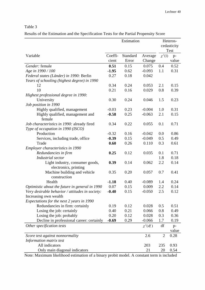
Table 3 presents the results of the maximum likelihood estimation of the partial propensity

score, specified as a probit model, as well as the results of various specification tests.

Although this estimation is only a by-product for the final evaluation a brief look at the results

is nevertheless interesting. They suggest that women are more likely to participate in CTRT.

That is not surprising because women experience far more unemployment than men during

the post-unification period. However, this partial correlation cannot be observed for highly

qualified women. Older persons are ceteris paribus less likely to be observed in CTRT. This is

also not surprising since participants are on average three years younger than nonparticipants.

Individuals who expect redundancies in the firm (in 1990) are more likely to be participants.

There appears to be also significant heterogeneity across different professions / occupations

Lechner 19

and industrial sectors. Finally, the negative coefficient of the variable that measures that the

individual expects a decline in the professional career appears to be counter-intuitive, whereas

the negative coefficient for individuals who believe that increasing one’s own wealth is a very

desirable behavior in a society may be due to a lower unemployment probability for these

probably well-motivated individuals.

< Table 3 about here >

Since the goal of the estimation is to obtain a consistent estimate of 0βV , testing the validity

of the preferred specification is important. First, all variables that are not contained in Table

3, but described in Table A.1 (see endnote 15), as well as different functional forms for the

continuous variables and interaction terms between Gender and variables related to job

position and education are subjected to score tests against omitted variables. None of them

appears to be significantly missing at the 5 percent level. Most results are above the 10

percent level.21 The results of the other specification tests do not provide any evidence against

the chosen specification: The last two columns of Table 3 do not contradict the assumption of

conditional homoscedasticity. Furthermore, the normality test as well as the information

matrix tests do not reject.22

C. Nonparametric estimation of causal effects and matching

This section summarizes the nonparametric methods used to estimate the causal effects of

CTRT as discussed by Lechner (1999). The reader is referred to that paper for more details on

the estimation methods. The suggested estimator of the training effect for the trainees can be

written as follows:

(4) . )1|(ˆ)1|(ˆ)1|(ˆˆ =−===−= SYESYESYYE ctctNθ

Note that individual treatment effects remain unrestricted across participants. To ease notation

Lechner 20

assume that observations in the sample are ordered such that the first Nt observations get

CTRT, and the remaining (N-Nt) observations do not. An obvious estimator of the first part is

the sample mean of the output variable in the subsample of the trainees.

Given that CIA is valid, needs to be a consistent estimator for

. One possible estimator that is in principle easy to

compute and to implement in such a situation is the matching estimator proposed in the

statistics literature (for example Rosenbaum and Rubin 1983, 1985).

)1|(ˆ =SYE c

}1|)]( =Sx)(,0|[{ == bXbSYEE c

Nnβ̂ Nnv β̂

Nnv β̂ 0

23 The idea of matching is

to find for every treated observation a single comparison observation that is as close as

possible in terms of the balancing score. When an identical comparison observation is found,

the estimation of the average causal effect is unbiased. In cases of 'mismatches', it is often

plausible to assume that local regressions on these differences will remove the bias (see

Lechner 1999). Table 4 gives the exact matching protocol.

< Table 4 about here >

This matching algorithm is close to the one proposed by Rosenbaum and Rubin (1985) and

Rubin (1991) called "matching within calipers of the propensity score". They find that such a

protocol produces the best results in terms of 'match quality' (reduction of bias). The

difference here is that instead of using a fixed caliper-width for all observations, the widths

vary individually with the precision of the estimate v . The more precisely is

estimated, the smaller is the width. The rationale behind this is that when using the partial

propensity score for matching conditioning is on instead of βnv

Nnβ̂ Nβ̂

Nnβ̂

. Since the asymptotic

standard error of v resulting from the estimation of can be considerable, it can be

expected that by matching only approximately on v , but additionally also on some

components of v directly (those for which are a priori reasoning suggests that they are

Lechner 21

particularly important) as well as on m, a better match could be obtained. The widths are

chosen that large, because matching is not only on the partial propensity score and its

components, but also on additional variables. The linear index is used instead of the

bounded partial propensity score given by , because matching on the latter with a

symmetric metric leads to an undesirable asymmetry when Φ is close to 0 and 1,

depending on which side the comparison j is.

Nnv β̂

)ˆ( Nnv βΦ

)ˆ( Nnv β

Nβ̂

Nβ̂

pairs. The final rows in that table present the respective joint tests.

24

A requirement for a successful (that is bias removing) implementation of a matching

algorithm is a sufficiently large overlap between the distributions of the conditioning

variables in both subsamples. For the partial propensity score this can be checked by

comparing the distribution of V in the subsample of trainee and potential comparison

observations. Here, most of the mass of the distribution of the comparison observations is to

the left of the treated, but there is still overlap for (almost) all of the distribution of V in the

treated sample.25

Since there appears to be sufficient overlap, the next question to be answered is whether

matching balances the distribution of X in the CTRT and the matched comparison sample.

Table 5 presents results to check balancing for the time-constant variables used in the probit

estimation (time-varying variables are considered in the following section together with the

evaluation results). Column (2) gives the marginal means of the unmatched comparison

group, and columns (3) and (4) give the marginal means for the matched comparison group as

well as for the CTRT participants. The last two columns present the p-value for the tests

suggested by Rosenbaum and Rubin (1985). The ‘two-sample’ sample statistic (col. (5)) tests

whether the two samples come from distributions with the same mean, whereas the ‘paired’

statistics check whether there are systematic differences of the means within the matched

Lechner 22

< Table 5 about here >

Table 5 shows that matching remov for the variables that are

o

over

prove

of their paper Card and Sullivan (1988) used a similar approach: They match

r

r resulting from the matching algorithm outlined above, define the

es almost all differences

significant in the estimation. When there are significant differences, it is with respect t

variables that are insignificant in the probit.26 Indeed, in the next section it is shown that

the whole pre-CTRT period CTRT observations and comparison observations do not differ

significantly (with one exception to be discussed later). Nevertheless, it appears to be clear

from the various evidence that the problem for the matching algorithms is to find enough

well-educated persons with high unemployment probabilities. In conclusion, the matching

algorithm provides an acceptable match, that is however not perfect. Therefore, the

econometric correction mechanism described in Lechner (1999) could be useful to im

the estimates.

In the first part

treated and comparison observations regarding their pre-training employment history. They

are in a worse position, because these variables are subject to considerable measurement erro

in their data. Besides, they ignore the kind of variables that enter the partial propensity score

in this analysis. Therefore, it is not surprising that they find this kind of conditioning

insufficient to yield unbiased estimates and switch to a model-based approach.

D. Evaluation

To describe the estimato

differences in matched pairs in the sample as Δy y yn nt

jc= − , Δb xn( ) = b x b xn

tjc( ) ( )− ,

n N t= 1,..., , where y jc and x j

c denote values o tio

ating in C RT th is matched to the treated (CTRT) observation n. The estimate

of the average causal effect and the respective standard error are computed as:

f an observa n from the pool of individuals

not particip T at

Lechner 23

(5) )(1)ˆ(,1ˆ 22

1ctt

t

t yytN

N

nntN N

VaryN

Ψ+Ψ=Δ= ∑=

θθ .

2ty

Ψ and denote the square of the empirical standard deviation of Y in the CTRT sample

and in the sample matched to the CTRT-sample, respectively.

2cy

Ψ

27 As mentioned in the previous

section, when a perfect match is achieved, implying that Δb xn( ) = 0 n N t= 1,...,, , these

estimates are consistent (see Rosenbaum and Rubin 1983). When the sample is large enough

the normal distribution can be used to perform tests and compute confidence intervals.

Following the objective of the program the focus is on outcome variables measuring

unemployment for particular months after the completion of CTRT. Since CTRT may end at

different points in calendar time for different individuals this gives us an unbalanced panel (or

non-rectangular sample), namely the number of observations is decreasing the longer the time

span after the end of CTRT.28 In addition to the instantaneous effect for a particular period,

the accumulated effect of CTRT over that period is also estimated (as the sum of the

respective single period effects for those individuals observed over the whole period under

consideration; the variance estimates takes the correlation of the single period effects into

account).

The results are given in Figure 2 and Table 6. Figure 2 shows the differences of

unemployment rates between the CTRT group and the comparison group. The mean effect

(solid line; + for the mismatch-corrected estimate) and its 95 percent pointwise confidence

interval based on the normal approximation (dashed line; ∇, Δ for the mismatch corrected

estimates) up to 24 months before CTRT and up to about 40 months after CTRT are

displayed. Since the number of observations decreases the longer the distance to the incidence

of CTRT is (see Table 6), the variance increases over post-CTRT time. This is reflected in the

widening of the confidence intervals. However, the accuracy of the estimated intervals itself

Lechner 24

may deteriorate, because the normal distribution may be not a good approximation of the

sample distribution of the mean anymore. Additionally, a mismatch correction may be

impossible or very imprecise, because there may be too few observations to identify and

estimate the parameters of the ordered probit model. Hence, on the very right hand side of

Figure 2 the results have to be interpreted with care (the collapse of the intervals on the very

right should be ignored because it is based on very few observations that happen not to vary

at all).

< Figure 2 about here >

The parts of Figure 2 to the left of the zero vertical mark (prior to CTRT) allow a judgement

about the quality of the matches concerning that particular variable.29 Although the number of

unemployed persons is generally higher in the CTRT sample, it is only in the month just prior

to CTRT that the difference is just significant (t-value: 1.95)

< Table 6 about here >

Figure 2 also shows that the immediate effect of CTRT is additional unemployment in the

months following the end of CTRT. After some months these negative effects disappear.

Indeed Table 6, that contains also the effects of CTRT with respect to full-time employment,

shows that the total effect for unemployment cannot be distinguished from zero after 24

months (12 months for full-time employment). At first sight this seems surprising, because

Figure 1 shows that the unemployment rate of CTRT participants is indeed falling rapidly

during the first 12 months after CTRT. However, there seems to be a simple explanation for

this effect. Recall that more than 50 percent of CTRT participants are unemployed before

CTRT. For an unemployed person the immediate effect of (full-time) CTRT is that during

CTRT his or her search efforts will be reduced (mean duration is 12 months!) compared to the

comparison nonparticipants. The results suggest that if there is a positive effect of CTRT it is

Lechner 25

not large enough to compensate for this initial negative outcome, and to be detected by the

estimator (note that the confidence bands are wide enough to make it difficult to exclude the

possibility of medium sized positive effects after about one year as well as of negative effects

of CTRT).

These general findings are confirmed by considering as outcome variables the receipt of

unemployment benefits, short-time work and unemployment together, or full-time

employment. Results from a sample of individuals who are either unemployed or on short-

time work before CTRT sharpen these conclusions.

When earnings are considered as an outcome variable, the same conclusions are obtained: a

very good match prior to training and no significant effect after training.30 Other results are

computed for different outcome variables that measure status or subjective prospects on the

labor markets, such as job position, expectations about a possible job loss in the next two

years, and whether one is very worried about keeping the current job. Additionally, there is

information on whether individuals expect an improvement or a worsening of the current

career position. With one exception there are no significant effects for all these variables. The

exception is the variable measuring subjective career perspectives in the next two years.

Although the effect of CTRT is positive, it is only for the first year after CTRT (mildly)

significant.

When training programs are very large, the estimates presented above could be contaminated

by so-called displacement effects or large program effect. This means that observations in the

comparison group are affected by the program because market interaction might lead to more

competition for them, thus depressing their earnings and reducing their employment

probabilities. Although there might also be an offsetting effect during the time when

participants are in CTRT and thus removed from the market, generally the former effect is

Lechner 26

expected to dominate at least in the longer term. It would lead to an estimate of the effects of

CTRT that is 'too positive'. However, since the effects of CTRT are estimated to be close to

zero in this paper, such a potential bias is not a problem with respect to the conclusion that

CTRT appears to be ineffective in lowering the risk of unemployment and increasing earnings

(it might even strengthen that conclusion).

E. Sensitivity

In addition to the already-mentioned issues, the sensitivity of the results is checked in several

other directions.

First, the perspective of time is changed: instead of considering a period after the end of

CTRT, pre- and post CTRT outcomes are compared and averaged for the same month / year

in calendar time. This does not lead to different conclusions.

To check whether the average treatment effects differ in specific subgroups of participants,

the sample is split according to gender, job position, occupational degree, age, and pre-

training employment status. Furthermore different subsamples defined by characteristics of

CTRT (start dates, end dates, duration, multiple spells of CTRT) are considered. No

significant differences appear.31

To check whether the so-called contamination bias (for example Heckman and Robb 1985),

meaning that the comparison group gets some other sort of training as a substitute for CTRT,

might be a problem, new comparison and CTRT samples (about 75 percent of all participants)

are selected. Observations in these samples either get no continuous training at all, or obtain

only CTRT. Again, no significant differences appear.

Another concern might be the use of a nonrectangular sample due to different end dates and

panel attrition. Therefore, a subsample of participants that are observed for at least 24 months

after the end of CTRT is selected. The results for this subsample mirror very closely the

Lechner 27

results presented in the previous section.

The already-mentioned alternative ways to handle the issue of time-varying start dates

(random, inflated) could be an issue. With respect to match quality, random assigns

significantly too few unemployment persons into the matched comparison group. Inflated

does not have this problem and produces a fairly balanced comparison sample (due to the

increased number of comparison observations). The results are similar to those reported in the

previous section. The only difference for both approaches is that the effect on the already-

mentioned variable measuring expected improvements in the job position in the next two

years is positive (as before) and now highly significant for the first year after CTRT. For

inflated it is positive and significant for the second year after CTRT as well.

Finally, for the yearly variables all computations are performed using the appropriate panel

weights. However, since there are only minor differences among weighted and unweighted

estimates, the former are not computed for the monthly data.

In conclusion the sensitivity analysis shows a remarkable stability of the results.

V. Conclusion

The general findings of the paper suggest that there are no positive earnings and employment

effects of public-sector-sponsored continuous vocational training and retraining (CTRT) in

East Germany at least in the short-run. Regarding the risk of unemployment there are negative

effects of CTRT directly after training ends. However, these negative effects fade out over the

first year after training. It is an open question whether the lack of a positive effect is due to a

bad signal participants send to prospective employers, or whether it is due to a lack of quality

in a narrower sense. Nevertheless, the results in this paper provide no justification of the large

expenditure for CTRT until 1993. The results are compatible with the claim that CTRT was

Lechner 28

very much a waste of resources, providing quantity without sufficient quality (or a

sufficiently positive signal). The quality problem has been realized by the labor office, which

subsequently tried to improve quality and changed the selection process to include a higher

share of individuals previously unemployed in CTRT. It should be noted that the lack of

measurable success of the programs appears despite the fact that participants are in general

well educated and had fairly high job positions in the GDR. Therefore, it is not the typical

low-skill-low-ability group that is the target of many government programs in the US and

Western Europe.

The overall negative picture may be an exaggeration of the real situation for several reasons:

Firstly, money spent for CTRT in the first two to three years may be seen as investments in

the East German training infrastructure, that had to be build from scratch. In this sense future

CTRT might still yield some returns on these early investments. Secondly, the massive use of

CTRT achieved a significant reduction of the official unemployment rate. This was politically

desired, and hence it might be seen as an achievement per se, although there might have been

cheaper ways to achieve this goal.

Although the data and the suggested nonparametric estimation strategy appeared to be well

suited for the problem at hand, the small sample remains a problem. It is mainly reflected in

comparatively large standard errors. Therefore, future research should investigate these

effects with different data sources, ideally ones that are larger but not less informative than

the GSOEP. Additionally, one might investigate jointly the effects of different types of

training, such as on-the-job training versus off-the-job training, or publicly-funded versus

privately-funded training. Likewise, it will be an issue whether the quality of the publicly-

funded training did really improve after 1992, as claimed by official sources.

Lechner 29

References

Angrist, J.D., and A.B. Krueger. 1999. "Empirical Strategies in Labor Economics."

Forthcoming in Handbook of Labor Economics, ed. O. Ashenfelter and D. Card, vol. 3,

Chapter 23.

Ashenfelter, O. 1978. "Estimating the Effect of Training Programs on Earnings." The Review

of Economics and Statistics 60:47-57.

Ashenfelter, O., and D. Card. 1985. "Using the Longitudinal Structure of Earnings to Estimate

the Effect of Training Programs." The Review of Economics and Statistics 67:648-660.

Bera, A., C. Jarque, and C.F. Lee. 1984. "Testing the Normality Assumption in Limited

Dependent Variable Models." International Economic Review 25:563-578.

Blaschke, D., and E. Nagel. 1995. "Beschäftigungssituation von Teilnehmern an AFG-

finanzierter beruflicher Weiterbildung." MittAB 2/95:195-213.

Bundesanstalt für Arbeit. 1992. Förderung der beruflichen Weiterbildung: Bericht über die

Teilnahme an beruflicher Fortbildung, Umschulung und Einarbeitung im Jahr 1991.

Nürnberg.

Bundesanstalt für Arbeit. 1993a. Förderung der beruflichen Weiterbildung: Bericht über die

Teilnahme an beruflicher Fortbildung, Umschulung und Einarbeitung im Jahr 1992.

Nürnberg.

Bundesanstalt für Arbeit. 1993b. Geschäftsbericht 1993. Nürnberg.

Bundesanstalt für Arbeit. 1994a. Berufliche Weiterbildung: Förderung beruflicher

Fortbildung, Umschulung und Einarbeitung im Jahr 1993. Nürnberg.

Bundesanstalt für Arbeit. 1994b. Geschäftsbericht 1994. Nürnberg.

Bundesanstalt für Arbeit. 1995. Berufliche Weiterbildung: Förderung beruflicher

Lechner 30

Fortbildung, Umschulung und Einarbeitung im Jahr 1994. Nürnberg.

Bundesminister für Arbeit und Sozialordnung. 1991. Übersicht über die Soziale Sicherheit,

Textergänzung Kapitel 26:Übergangsregelungen für die neuen Bundesländer. Bonn.

Bundesministerium für Bildung und Wissenschaft. 1994. Berufsbildungsbericht 1994. Bad

Honnef: Bock.

Bundesministerium für Wirtschaft. 1995. Dokumentation, Nr. 382.

Buttler, F., and K. Emmerich. 1994. "Kosten und Nutzen aktiver Arbeitsmarktpolitik im

ostdeutschen Transformationsprozeß." In Schriften des Vereins für Sozialpolitik 239/4:61-

94.

Card, D., and D. Sullivan. 1988. "Measuring the Effect of Subsidized Training Programs on

Movements in and out of Employment." Econometrica 56:497-530.

Dagenais, M.G., and J.M. Dufour. 1991. "Invariance, Nonlinear Models, and Asymptotic

Tests." Econometrica 59:1601-1615.

Davidson, R., and J.G. MacKinnon. 1984. "Convenient Specification Tests for Logit and

Probit Models." Journal of Econometrics 25:241-262.

Dehejia, R., and S. Wahba. 1995. "A Matching Approach for Estimating Causal Effects in

Non-Experimental Studies.” Mimeo.

[DIW] Deutsches Institut für Wirtschaftsforschung. 1994. Wochenbericht 31/94. Berlin.

Fitzenberger, B., and H. Prey. 1997. "Assessing the Impact of Training on Employment: The

Case of East Germany." IFO Studien 43:71-116.

Friedlander, D., D.H. Greenberg, and P.K. Robins. 1997. "Evaluating Government Training

Programs for the Economically Disadvantaged." Journal of Economic Literature 35:1809-

1855.

Lechner 31

Gu, X.S., and P.R. Rosenbaum. 1993. "Comparison of Multivariate Matching Methods:

Structures, Distances, and Algorithms." Journal of Computational and Graphical Statistics

2:405-420.

Heckman, J.J., H. Ichimura, and P. Todd. 1998. "Matching as an Econometric Evaluation

Estimator." Review of Economic Studies 65:261-294.

Heckman, J.J., and V.J. Hotz. 1989. "Choosing Among Alternative Nonexperimental

Methods for Estimating the Impact of Social Programs: The Case of Manpower Training."

Journal of the American Statistical Association 84:862-880 (includes comments by

Holland and Moffitt and a rejoinder by Heckman and Hotz).

Heckman, J.J., R.J. LaLonde, and J.A. Smith. 1999. "The Economics and Econometrics of

Active Labor Market Programs." Forthcoming in Handbook of Labor Economics, ed. O.

Ashenfelter and D. Card, vol. 3.

Heckman, J.J., and R. Robb. 1985. "Alternative Methods of Evaluating the Impact of

Interventions." In Longitudinal Analysis of Labor Market Data, ed. J.J. Heckman and B.

Singer. New York: Cambridge University Press 156-245.

Heckman, J.J., and J.A. Smith. 1999. "The Pre-Program Dip and the Determinants of

Participation in a Social Program: Implications for Simple Program Evaluation Strategies."

In The Economic Journal 109:313-348.

Holland, P.W. 1986. "Statistics and Causal Inference." Journal of the American Statistical

Association 81:945-970 (includes comments by Cox, Granger, Glymour, Rubin).

Hübler, O. 1994. "Weiterbildung, Arbeitsplatzsuche und individueller Beschäftigungsumfang

- eine ökonometrische Untersuchung für Ostdeutschland." Zeitschrift für Wirtschafts- und

Sozialwissenschaften 114: 419-447.

Lechner 32

Hübler, O. 1997. "Evaluation beschäftigungspolitischer Maßnahmen in Ostdeutschland."

Jahrbücher für Nationalökonomie und Statistik 216:21-44.

[IAB] Institut für Arbeitsmarkt- und Berufsforschung. 1995. Zahlen-Fibel 1995 (BeitrAB

101). Nürnberg.

LaLonde, R.J. 1986. "Evaluating the Econometric Evaluations of Training Programs with

Experimental Data." American Economic Review 76:604-620.

LaLonde, R.J. 1995. "The Promise of Public Sector-Sponsored Training Programs." Journal

of Economic Perspectives 9: 149-168.

Lechner, M. 1999. “Earnings and Employment Effects of Continuous Off-the-Job Training in

East Germany after Unification.” Journal of Business & Economic Statistics 17:74-90.

Orme, C. 1988. "The Calculation of the Information Matrix Test for Binary Data Models."

The Manchester School 56:370-376.

Pannenberg, M. 1995. Weiterbildungsaktivitäten und Erwerbsbiographie. Frankfurt: Campus.

Pannenberg, M., and C. Helberger. 1995. "Kurzfristige Auswirkungen staatlicher

Qualifizierungsmaßnahmen in Ostdeutschland: Das Beispiel Fortbildung und

Umschulung." Schriftenreihe des Vereins für Sozialpolitik.

Rosenbaum, P.R. 1984. "From Association to Causation in Observational Studies: The Role

of Tests of Strongly Ignorable Treatment Assignment.” Journal of the American Statistical

Association 79:41-48.

Rosenbaum, P.R., and D.B. Rubin. 1983 "The Central Role of the Propensity Score in

Observational Studies for Causal Effects." Biometrica 70:41-50.

Rosenbaum, P.R., and D.B. Rubin 1985. "Constructing a Comparison Group Using

Multivariate Matched Sampling Methods That Incorporate the Propensity Score." The

Lechner 33

American Statistician 39:33-38.

Rubin, D.B. 1974. "Estimating Causal Effects of Treatments in Randomized and

Nonrandomized Studies." Journal of Educational Psychology 66:688-701.

Rubin, D.B. 1977. "Assignment of Treatment Group on the Basis of a Covariate." Journal of

Educational Statistics 2:1-26.

Rubin, D.B. 1979. "Using Multivariate Matched Sampling and Regression Adjustment to

Comparison Bias in Observational Studies." Journal of the American Statistical

Association 74:318-328.

Rubin, D.B. 1991. "Practical Implications of Models of Statistical Inference for Causal

Effects and the Critical Role of the Assignment Mechanism." Biometrics 47:1213-1234.

Sobel, M.E. 1994. "Causal Inference in the Social and Behavioral Sciences." In Handbook of

Statistical Modeling for the Social and Behavioral Sciences, ed. G. Arminger, C.C. Clogg

and M.E. Sobel. New York: Plenum Press.

Statistisches Bundesamt. 1994. Statistisches Jahrbuch für die Bundesrepublik Deutschland,

1994. Stuttgart: Metzler-Pöschel.

Wagner, G.G., R.V. Burkhauser, and F. Behringer. 1993. "The English Language Public Use

File of the German Socio Economic Panel." Journal of Human Resources 28:429-433.

White, H. 1982. "Maximum Likelihood Estimation of Misspecified Models." Econometrica

50:1-25 "Corrigendum", Econometrica 51:513.

Endnotes

Lechner 34

1. There was a considerable policy shift during 1993. This paper concentrates on the regime

that was valid before April 1993.

2. Heckman and Hotz (1989) dispute some of the pessimistic claims by LaLonde (1986).

3. There are more studies published in German (for example Pannenberg and Helberger 1995;

Pannenberg 1995; Hübler 1994, 1997).

4. The training variable is from a special training sub-survey of the GSOEP collected in 1993.

5. The data used in this section is based - unless indicated otherwise - on information

contained in Statistisches Bundesamt (1994), DIW (1994), Bundesanstalt für Arbeit (1994a,

1994b), Bundesministerium für Bildung und Wissenschaft (1994), Bundesministerium für

Wirtschaft (1995), and Bundesminister für Arbeit und Sozialordnung (1991).

6. Short-time work ("Kurzarbeit") is a reduction of individual working hours accompanied by

a subsidy from the labor office to compensate employees for most of the occurring earnings

loss.

7. The definition of full-time work used here includes about 5-10% individuals in ABM. The

statistics quoted in this paragraph are computed from the GSOEP, that will be described in the

next section.

8. Unemployment, short-time work, and CTRT numbers are lower than the official ones for

the total population, because of the age restriction and because of different definitions of the

relevant populations. Furthermore, CTRT includes only individuals receiving compensation

for potential earnings losses.

9. Our own interviews with selected job counselors at the local level confirm the view that

between 1990 and 1993 the supply of CTRT was not significantly rationed.

Lechner 35

10. For an English language description of the GSOEP see Wagner, Burkhauser, and

Behringer (1993).

11. Younger than 53 in 1993 for the nonparticipants.

12. CTRT was sometimes used to ‘bridge’ the gap to early retirement.

13. However, note that not only the comparison is not valid because of the inclusion of

subsidies to employers to provide on-the-job training for individuals facing difficult labor

market conditions in the official numbers, but also that there are issues related to the

questionnaire (retrospective calendar): (1) participants may forget very short training spells;

(2) respondents may not bother to tick boxes for a particular month in case of very short spells

of a few days; (3) multiple spells are added (10 percent).

14. See Buttler and Emmerich (1994), Blaschke and Nagel (1995), IAB (1995), p. 134.

15. See Table A.1 in the data appendix that can be downloaded from my the publications part

of my homepage (www.siaw.unisg.ch/lechner).

16. See Holland (1986) and Sobel (1994) for an extensive discussion of concepts of causality

in statistics, econometrics, and other fields.

17. As a notational convention big letters indicate quantities of the population or of members

of the population and small letters denote the respective quantities in the sample. Sample units

(n=1,...,N) are supposed to come from N independent draws in this population.

18. In the language of regression-type approaches such a variable leads to simultaneity bias.

19. For these considerations, it does not matter how the labor market really works, but how

the individual (and / or the labor office) believes it to work at the time of the participation

decision. There might be substantial differences between actual and expected outcomes

Lechner 36

because individuals are used to the rules of a former command type economy. Furthermore,

rapid changes after unification make correct predictions difficult.

20. See also Heckman and Smith (1999) for the USA.

21. The standard errors and the score tests against heteroscedasticity and omitted variables are

computed using the GMM (or PML) formula given in White (1982). Five versions are

computed: (i) based on the matrix of the outer product of the gradient (OPG) alone, (ii) on the

empirical hessian alone, (iii) on the expected hessian alone, (iv) and on the product (hessian)-1

OPG (hessian)-1, (v) respectively on (expected hessian)-1 OPG (expected hessian)-1. Previous

Monte Carlo studies (for example Davidson and MacKinnon 1984) as well as theoretical

papers (for example Dagenais and Dufour 1991) suggest that tests based on the latter avoid

some problems that can occur with other versions. Therefore, the results presented are

computed using (v).

22. Conditional homoscedasticity and normality of the probit latent error terms are tested

using conventional specification tests (Bera, Jarque and Lee 1984; Davidson and MacKinnon

1984; White 1982). The information matrix tests statistics (IMT) are computed using the

second version suggested in Orme (1988) that appeared to have good small sample properties.

Only main-diagonal indicators refers to the IMT using as test indicators only the main

diagonal of the difference between OPG and expected hessian.

23. Suitably refined nonparametric regressions could also be used. However, given the sample

size and the high dimensional balancing score with many discrete components, nonparametric

regressions will be subject to the typical curse of dimensionality.

24. Note that this matching method does not appear to fulfill any optimality condition: Match

quality could be increased (namely the bias reduced) by using the same comparison

Lechner 37

observations more than once (namely increase the variance). But on the other hand more than

one comparison observation could be assigned to any treated (reducing the variance,

increasing the bias). Optimal matching depends on the distribution of X (for example Gu and

Rosenbaum 1993). With the high dimension and the mixture of discrete and continuous

elements in X, it is not sensible to estimate its distribution with the current sample. The

selected algorithm is a compromise that is intuitively plausible and easy to implement.

25. The respective plot is contained in a previous version of the paper that can be downloaded

from my web page (www.siaw.unisg.ch/lechner).

26. Note that the joint test based on JW2 rejects as well. Note however that the estimate of the

variance of JW2 takes into account not only the distribution of X in the samples, but also the

exact pairing. If the match is (almost) exact for all pairs, then JW2 could be still very large

because its variance is shrinking, whereas JW1 will be (almost) zero. Since the exact pairing

is inessential for the balancing argument, JW1 seems the more appropriate statistic.

27. The variance estimate exploits the fact that the algorithm only chooses an observation

once.

28. There is also some panel attrition contributing to this effect.

29. Testing whether these lines deviate significantly from zero is similar to tests suggested by

Rosenbaum (1984) to use unaffected outcomes (in his terminology) or to try to invalidate

CIA. They are called pre-program tests by Heckman and Hotz (1989) and others.

30. These results are also contained in the already-mentioned previous version of the paper

available at www.siaw.unisg.ch/lechner.

31. However, the power of these tests could be rather small because of the smaller samples.

Lechner 38

Table 1

Entries into Continuous Vocational Training and Retraining 1991 to 1993

1991 1992 1993

Entries x1000

Share in Percent

UE t-benefits

Entries x1000

Share in Percent

UE t-benefits

Entries x1000

Share in Percent

UE t-benefits

CT (long) 442 35a n.a. 462 70 85b 182 74 82a

CT (short) 187 100 n.a. 129 100 85b 0c - -

Retraining 130 35 a n.a. 183 81 85b 81 91 82a

Source: Bundesanstalt für Arbeit (1992, 1993a, 1993b, 1994a, 1995), own computations.

Note: Total employment fell from 7.2 million in 1991 to 6.1 million in 1993. The

unemployment rate increased from 10 percent in 1991 to 16 percent in 1993.

UE: unemployed before entering; t-benefits: recipient of t-benefits ("Grosses Unterhaltsgeld";

earnings replacement); CT: continuous training; short: very short term courses for the

unemployed to improve their job search skills (§41a Work Support Act), long: all other

continuous training; n.a.: not available

a. aggregated over 2 categories

b. aggregated over all categories

c. program stopped

Lechner 39

Table 2

Expenditure of the Labor Office for CTRT 1991 to 1993

1991 1992 1993

t-benefits in billion DM 1.6 6.0 6.6

Other expenditure in billion DM 2.7 4.7 3.7

Institutional support in billion DM 0.2 0.1 0.1

Total expenditure for CTRT in billion DM 4.4 10.8 10.4

Share of CTRT expenditures in total expenditure of labour offices in East Germany

15 % 23 % 21 %

Source: Bundesanstalt für Arbeit (1995), Table 34, own calculations.

Note: Spending for subsidies to employers to provide on-the-job training for individuals

facing difficult labor market conditions is excluded.

Lechner 40

Table 3

Results of the Estimation and the Specification Tests for the Partial Propensity Score

Estimation Heteros-cedasticity

Test Variable Coeffi-

cient Standard

Error Average Change

χ 2 1( )

p-value

Gender: female 0.51 0.15 0.075 0.4 0.52 Age in 1990 / 100 -1.95 0.62 -0.093 1.1 0.31 Federal states (Länder) in 1990: Berlin 0.27 0.18 0.042 Years of schooling (highest degree) in 1990

12 0.34 0.24 0.053 2.1 0.15 10 0.21 0.16 0.029 0.8 0.39

Highest professional degree in 1990: University 0.30

0.24

0.046

1.5

0.23

Job position in 1990 Highly qualified, management -0.03 0.23 -0.004 1.0 0.31 Highly qualified, management and

female -0.58 0.25 -0.063 2.1 0.15

Job characteristics in 1990: already fired 0.34 0.22 0.055 0.1 0.71 Type of occupation in 1990 (ISCO)

Production -0.32 0.16 -0.042 0.0 0.86 Services, including trade, office -0.39 0.15 -0.049 0.5 0.49 Trade 0.60 0.26 0.110 0.3 0.61

Employer characteristics in 1990 Redundancies in firm 0.25 0.12 0.035 0.1 0.71 Industrial sector 1.8 0.18

Light industry, consumer goods, electronics, printing

0.39 0.14 0.062 2.2 0.14

Machine building and vehicle construction

0.35 0.20 0.057 0.7 0.41

Health -1.18 0.40 -0.089 1.4 0.24 Optimistic about the future in general in 1990 0.07 0.15 0.009 2.2 0.14 Very desirable behavior / attitudes in society: Increasing own wealth

-0.40 0.15 -0.050 2.5 0.12

Expectations for the next 2 years in 1990 Redundancies in firm: certainly 0.19 0.12 0.028 0.5 0.51 Losing the job: certainly 0.40 0.21 0.066 0.8 0.49 Losing the job: probably 0.20 0.12 0.028 0.3 0.36 Decline in professional career: certainly -0.69 0.29 -0.066 1.7 0.19

Other specification tests χ 2( )df df p- value

Score test against nonnormality 2.6 2 0.28 Information matrix test

All indicators 203 235 0.93 Only main diagonal indicators 21 20 0.54

Note: Maximum likelihood estimation of a binary probit model. A constant term is included

Lechner 41

in the model. N = 1411 (1280 controls). The tests are explained in footnotes 20 and 21. Bold

letters: t-value larger than 1.96 in absolute value. Average change denotes the average (finite)

change in the probabilities when a single dummy variable is changed from zero to one and

when age is increased by one year (without changing the values of the other variables).

Averaging is over the empirical distribution of all over explanatory variables.

Lechner 42

Table 4

Matching Algorithm

Step 1 Split observations in two exclusive pools according to participation status (T-pool and C-pool).

Step 2 Draw randomly an observation in T-pool (denoted by n) and remove from T-pool. Step 3 Define caliper of partial propensity score for observation n in terms of the

predicted index v and its conditional variance Var (derived from by the delta method).

Nn β̂ )|ˆ( nN vVV =β

)ˆ( NVar βStep 4 Find observations in C-pool (denoted by j) obeying ∈Njv β̂ ])ˆ(ˆ[ Nnv β ± NnvVarc β

ˆNjv β

. The constant c is chosen such that the interval is identical to a 95% confidence interval around . Nnv β̂

Step 5 (a) If there are fewer than two observations in this interval: Find observation j in C-pool that is closest to observation n, such that it minimizes 2)ˆ( Nnv β− .

(b) If there are two or more observations in this set generated by Step 4: Take these observations and compute the variables m in relation to the start date of observation n. Denote these and perhaps other variables already included in V as ~mj and ~mn , respectively. Define a distance between each comparison observation j and n as d j n( , ) = −′)~,ˆ( jN mβ ′)jv ~,ˆ( nNn mβ . Choose a comparison observation j with the smallest Mahalanobis distance )) njWd′

v

,(,(),( njdnj =ξ within the caliper. W denotes the inverse of the estimated variance of )′~,ˆ(vβ in the C-pool.

mN

Step 6 Remove j from C-pool. Step 7 If there are any observations in the T-pool left, start again with step 2. Note: The asymptotic standard error of is in the range from 0.14 to 0.50 (mean and

median: 0.25; standard deviation 0.06) in the CTRT sample, and from 0.14 to 0.52 (0.25;

0.23; 0.08) in the comparison sample (before matching).

v-variables used for the additional conditioning are: gender, university degree, 12 and 8 years

of schooling, highly qualified or management job position (1990), women in highly qualified

or management job positions (1990), expect to be laid off (1990), working in industrial

sectors light industry, machine building and vehicle construction (1990). The additional v-

variables are included in the list of matching variables as an additional safeguard against

inconsistent estimation of v . m-variables are: expectation of losing own job in the next two

years (yearly), expectation of a declining career in the next two years (yearly), monthly wage

/ salary (yearly), training (unspecified, yearly), self-employment (yearly), highly qualified or

management job positions (yearly), unemployment (monthly), short-time work (monthly), full-

Nnv β̂

Nβ̂

Lechner 43

time work (monthly). For each monthly m-variable the status in the month just prior to CTRT,

the average over the four months prior to CTRT and the average over all months after June

1990 are used. For each yearly variable the status in the last interview and the status in the

interviews before that are used.

Lechner 44

Table 5

Descriptive Statistics and Tests for Balancing for Variables Included in the Partial Propensity

Score

All Controls (1280)

Matched Controls

CTRT Two Sample

Test

Paired Test

(1) (2) (3) (4) (5) (6) Variable Mean or Share in Percent p-value p-value Gender: female 41 52 58 0.37 0.21 Age in 1990 37 35 34 0.64 0.61 Federal states (Länder) in 1990: Berlin 7 8 12 0.39 0.32 Years of schooling (highest degree) 1990

12 16 21 30 0.11 0.022 10 56 62 58 0.43 0.31

Highest professional degree in 1990: university

11 13 20 0.17 0.046

Job position in 1990 Highly qualified, management 20 16 26 0.058 0.004 Highly qualified, management and

female 10 5 9 0.21 0.096

Job characteristics in 1990: already fired 3 9 11 0.67 0.66 Type of occupation in 1990 (ISCO)

Production 40 43 23 0.002 0.0003 Services, incl. trade, office 25 20 21 0.87 0.86 Trade 4 6 6 1 1

Employer characteristics in 1990 Redundancies in firm 43 76 67 0.12 0.048 Industrial sector

Light ind., consumer goods, electronics, printing

15 38 31 0.23 0.12

Machine building and vehicle construction

5 6 9 0.33 0.15

Health 7 1 1 1 1 Optimistic about the future in general in

1990 18 13 14 0.85 0.85

Very desirable behavior / attitudes in society: increasing own wealth 30 21 14

0.18

0.12

Expectations for the next 2 years in 1990 Redundancies in firm: certainly 29 53 49 0.52 0.47 Losing the job: certainly 5 10 13 0.42 0.42 Losing the job: probably 33 57 45 0.072 0.052 Decline in professional career:

certainly 3 3 3 1 1

χ 2 ( )df df p-value Joint Wald test for two-sample mean difference (JW1)

21 0.22 0.50

Joint Wald test for paired mean difference (JW2)

53 0.21 0.0001

Lechner 45

Note: ; ;

.

denotes the value of a comparison observation matched to treated observation n. S2(a)

denotes the empirical variance of a. Asymptotically, should be good approximation

for the distribution of JW1 and JW2 when there are no systematic differences of the K

attributes given in the table for the matched pairs. For the computation of JW2 one variable is

deleted from the test because of an otherwise singular covariance matrix. The tests for single

variables in col. (5) and (6) are the respective analogs of JW1 and JW2.

bxsxsbNJW nnt 1

)(22 )]()(['1 −+=

∑=

−t

nn

N

n

kkt xxN1

)(/1)(

bxxsbNJW nnt 1

)(2 )](['2 −−=

)(2 Kχ

=kb

)(nx

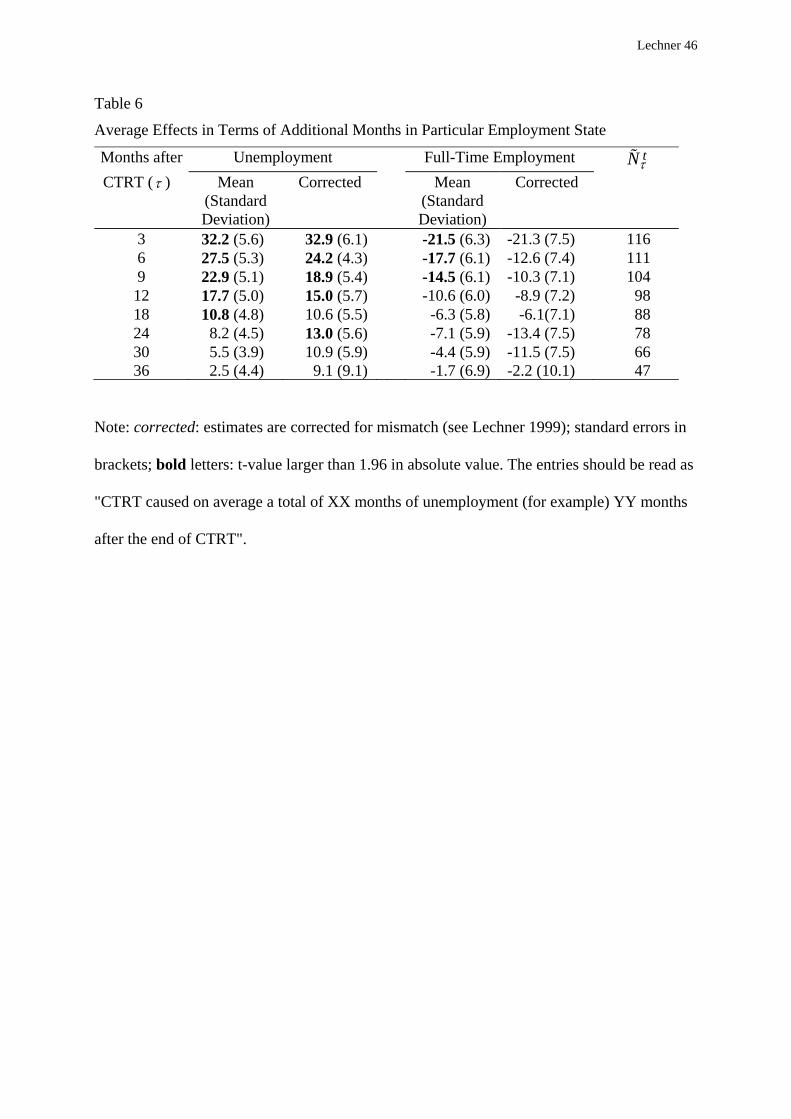
Lechner 46

Table 6

Average Effects in Terms of Additional Months in Particular Employment State

Months after Unemployment Full-Time Employment tNτ

CTRT (τ ) Mean (Standard Deviation)

Corrected

Mean (Standard Deviation)

Corrected

3 32.2 (5.6) 32.9 (6.1) -21.5 (6.3) -21.3 (7.5) 116 6 27.5 (5.3) 24.2 (4.3) -17.7 (6.1) -12.6 (7.4) 111 9 22.9 (5.1) 18.9 (5.4) -14.5 (6.1) -10.3 (7.1) 104 12 17.7 (5.0) 15.0 (5.7) -10.6 (6.0) -8.9 (7.2) 98 18 10.8 (4.8) 10.6 (5.5) -6.3 (5.8) -6.1(7.1) 88 24 8.2 (4.5) 13.0 (5.6) -7.1 (5.9) -13.4 (7.5) 78 30 5.5 (3.9) 10.9 (5.9) -4.4 (5.9) -11.5 (7.5) 66 36 2.5 (4.4) 9.1 (9.1) -1.7 (6.9) -2.2 (10.1) 47

Note: corrected: estimates are corrected for mismatch (see Lechner 1999); standard errors in

brackets; bold letters: t-value larger than 1.96 in absolute value. The entries should be read as

"CTRT caused on average a total of XX months of unemployment (for example) YY months

after the end of CTRT".

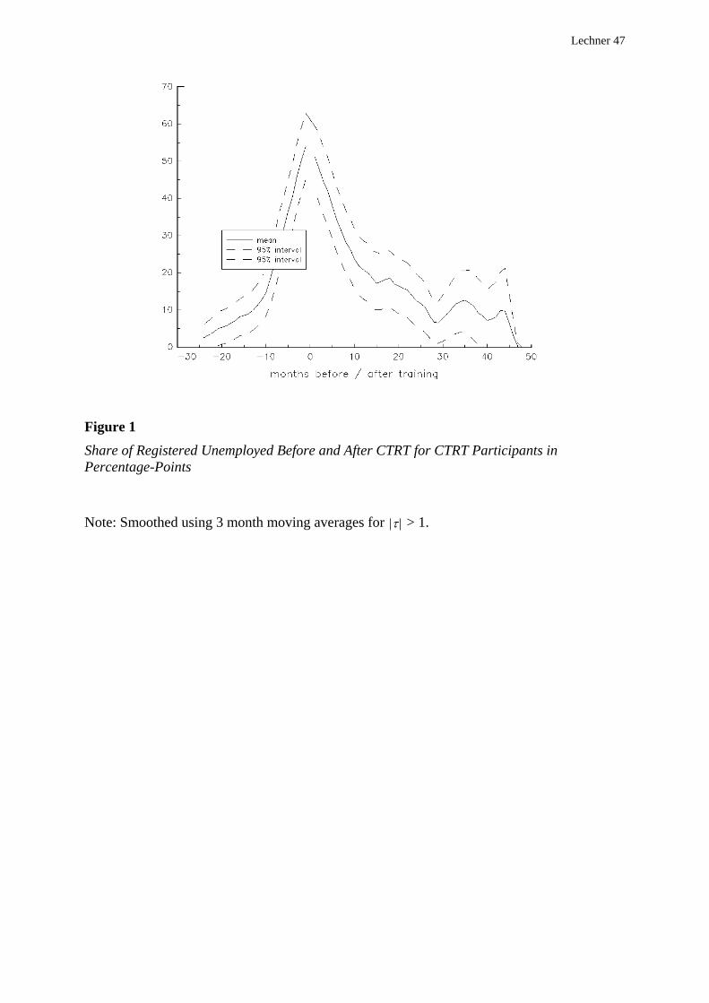
Lechner 47

Figure 1

Share of Registered Unemployed Before and After CTRT for CTRT Participants in Percentage-Points

Note: Smoothed using 3 month moving averages for | |τ > 1.

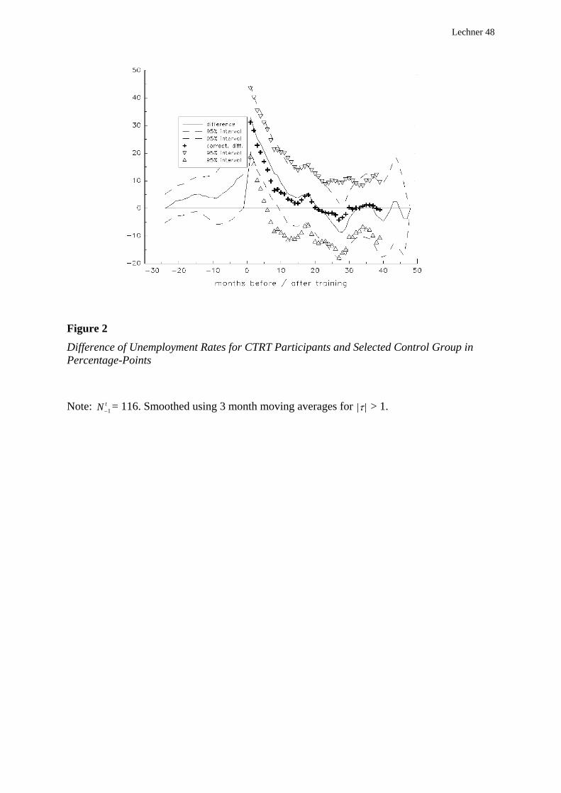
Lechner 48

Figure 2

Difference of Unemployment Rates for CTRT Participants and Selected Control Group in Percentage-Points

Note: = 116. Smoothed using 3 month moving averages for |N t−1 |τ > 1.