August 1991 Report No. STAN-CS-91-1377

Also Numbered CSL-TR-91-487

An Evaluation of Left-Looking, Right-Looking and MultifrontalApproaches to Sparse Cholesky Factorization on

Hierarchial-Memory Machines

bY

Edward Rothberg and Anoop Gupta

Department of Computer Science

Stanford University

Stanford, California 94305

Y

REPORT DOCUMENTATION PAGE fi-AoolovrdOM@ No. 07wot$$

IVW.--q l a mf-q a a t# -c m.---.wuwo uo b mtutk ,-o lr wo .@ o wn4 wm. I)l)m

-@-u81 .w~. M a wl.1. &GtNCY US8 OULV (Um-8 WakJ 2. UPON 01tl 1. awont TYPl AN0 OAT)$ (ovgn#o

1. TITLE AND su$TiTU An Evaluation of Left-Looking, Kight-Looklnar.ru~~~o)~~~lta)Ind Multifrontal Approaches to Sparse Cholesky Factorization 87-K-0828In Hierarchical-Memory Machines

L AUTHOR(S)A

Edward Rothberg and Anoop Gupta

I. PtRfORMINC ORCANlZATlON NAM(S) AN0 AOORtSS(tS) 8. Pf WORMING ORGANUATlONComputer Science Dept. rwoat WMBIRStanford University STAN-CS-91-1377Stanford, CA 94305-2140 CSL-TR-91-487

I. SPONSORING /I MONITORING AGtNCV NAME(S) AN0 AOORtSS(ES) lo. SPONSORING I MONITORINGAGtMCY MPORT NUMltR

DARPAArlington, VA

1. JUPPLtMfNtARY NOTtS.

128. OISTRI8UtlON / AVAILA8ILlTY STATfM[NT 12 b. olSTRl~Utl0N COOI

Unlimited

5. AB3lRACT (Mwmum ZOO wordt)

Abstract

In this paper we present 8 comprehensive analysis of the performance of a variety of sparse CholeSkyfactorization methods on hierarchical-manor-y machines. We investigate methods that vary along two diffelentaxes. Along the first axis, we consider three different high-level approaches to sparse factorization: left-looking, right-looking, and multifrontal. Along the second axis, we consider the implementation of each ofthese high-level approaches using different sets of primitives. The primitives vary based on the structures theymanipllate. One important structure in sparse Cholesky factorizafion is a single column of the matrix. Wefirst consider primitives that manipulate single columns. l%ese arc the most commonly used primitives forexpressing the sparse Cholesky computation. Another important structure is the supernode, a set of columnswith identical non-zero stmcturcs. We consider sets of primitives that exploit the supernodal structun of thematrix to varying degrees. We find that primitives that manipulate larger structures greatly increase the amountof exploitable data reuse, thus leading to dramatically higher performance on hierarchical-memory machines.We observe performance increases of two to three times when comparing methods based on primitives thatmake extensive use of the supernodal structure to methods based on primitives that manipulate columns. Wealso find that the overall approach (left-looking. right-looking, or multifrontal) is less important for performancethan the particulu set of primitives used to implement the approach.

14. $UOJtCT TlRMS 1% NUMBtI Of PAGtS

Hierarchical-memory machines, sparse Cholesky factorization 47L16. PRKf COOt

17. StCURlTY CLASSIFICATION - 1.. $~CU~rTV ClASSl~lCATlON 1s. SECWTY CUSSIWATION 10. LIMITATION Of A#STRACO f UPOat Of TMlt PAGt Of ADSTRACTUnclassified Unclassified Unclassified

cr.-m Itancarc~ Form 299 !Qev 2.89)

An Evaluation of Left-Looking, Right-Looking, and MultifrontalApproaches to Sparse Cholesky Factorization on

Hierarchical-Memory Machines

Edward Rothberg and Anoop GuptaDepartment of Computer Science

Stanford UniversityStanford, CA 94305

August 13, 1991

Abstract

In this paper we present a comprehensive analysis of the performance of a variety of sparse Choleskyfactorization methods on hierarchical-memory machines. We investigate methods that vary along two differentaxes. Along the first axis, we consider three different high-level approaches to sparse factorization: left-looking, right-looking, and muhi.frontal. Along the second axis, we consider the implementation of each ofthese high-level approaches using different sets of primitives. The primitives vary based on the structures theymanipulate. One important structure in sparse Cholesky factorization is a single column of the matrix. Wefirst consider primitives that manipulate single columns. These are the most commonly used primitives forexpressing the sparse Cholesky computation. Another important structure is the supemode, a set of columnswith identical non-zero structures. We consider sets of primitives that exploit the supernodal structure of thematrix to varying degrees. We find that primitives that manipulate larger structures greatly increase the amountof exploitable data reuse, thus leading to dramatically higher performance on hierarchical-memory machines.We observe performance increases of two to three times when comparing methods based on primitives thatmake extensive use of the supernodal structure to methods based on primitives that manipulate columns. Wealso find that the overall approach (left-looking, right-looking, or mu.ltifrontal) is less important for performancethan the particular set of primitives used to implement the approach.

1 Introduction

The Cholesky factorization of a large sparse positive definite matrix is an extremely important computation,arising in a wide variety of problem domains. This paper considers the performance of workstation-classmachines on this computation, using several different factorization methods. The performance of such machineshas been increasing rapidly, with workstation-class machines now performing dense matrix computations atsignificant fractions of the performance of vector supercomputers. Such machines have the potential to solvelinear algebra problems extremely cost-effectively.

Much research has been done on performing sparse Cholesky factorization efficiently. The performance ofthe computation is well understood for machines with simple memory systems (see, for example, [12]) andfor vector supercomputers (see [l, 3, 51). This paper instead focuses on the performance of sparse Choleskyfactorization on machines with hierarchical-memory systems. Memory hierarchies are crucial for building high-performance machines at low cost. They bridge the speed gap between extremely fast processors, whose speedis almost doubling every year, and the relatively slow main memories that must be used to keep costs down. Ifa computation can make good use of the hierarchy, then it can avoid the large latencies associated with fetchingdata from the slower levels of the hierarchy, yielding much higher performance. We look at several differentsparse Cholesky factorization methods, and consider how well each one uses the memory hierarchy.

The implementor of a sparse Cholesky factorization code faces a number of implementation decisions. Ourgoal in this paper is to study the impact of these decisions on the performance of the overall code on hierarchical-

1

memory machines. The first and probably most visible implementation decision we consider is the structureof the overall computation. We consider three approaches: left-looking, right-looking, and multifrontal. Theseapproaches will be summarized in the next section.

Another important implementation decision that we consider is the choice of primitives on which the com-putation is based The most commonly used primitives are column-column primitives, where columns of thematrix arc used to modify other columns. We demonstrate that column-column primitives yield low performanceon hierarchical-memory machines, primarily because they exploit very little data reuse. With such primitives,data items are fetched mainly from the more expensive levels of the memory hierarchy.

We next consider factorization methods based on supemode-column primitives. Such primitives take ad-vantage of the existence of sets of columns with identical non-zero structures, called supernodes, to increasedata reuse. These primitives modify columns of the matrix by all columns in an entire supemode at once. Theincreased reuse comes from the fact that the destination column is modilied a number of times, allowing thesupemode-column modification to be unrolled [7]. The unrolling allows data items from the destination to bekept in processor registers across multiple modifications. As a result, for moderately large sparse problems,memory reference are reduced by more than 50% and performance is improved by between 50% and 100%. Wealso consider column-super-node primitives, where a single column is used to modify a number of columns in asupemode. While the reuse benefits of such primitives are qualitatively similar to those of supernode-columnprimitives, the achieved benefits are much smaller.

We then consider primitives that modify a number of destination columns by a number of source columnsat once. We first look at a simple case, consisting of supernode-pair primitives, where pairs of columns aremodified by supernodes. Such methods further increase the amount of exploitable reuse. Memory references arereduced by another 35% from the supemode-column methods, and performance is improved by between 30% and45%. We then consider the use of supernode-supernode primitives, where supemodes modify entire supemodes.Such primitives allow the computation to be blocked, to increase reuse in the processor cache. Factorizationcodes based on these primitives further improve performance; we observe a 10% to 30% improvement oversupemode-pair codes.

Finally, we look at supernode-matrix primitives, where a supemode is used to modify the entire matrix. Themultifrontal method is typically expressed in such terms. Supemode-matrix primitives make even more datareuse available. We tind, however, that the impact of this increase is small; supemode-matrix methods yieldroughly the same performance as supemode-supemode methods. The reason is simply that supemode-supemodemethods exploit almost all of the available reuse. The amount of additional reuse exposed by supemode-matrixmethods is minor.

This paper makes the following contributions to the understanding of the sparse Cholesky computation.First, it compares a number of different methods using a consistent framework. For each method, we factorthe same set of benchmark matrices on the same set of machines, thus allowing for a more detailed analysisof the performance differences between the methods. This paper also provides a detailed study of the cachebehavior of the different methods. We study the impact of a number of cache parameters on the miss ratesof each of the factorization methods. Finally, this paper analyzes supernode-supemode methods, a class ofmethods that have so far received little attention. The use of supemode-supemode primitives has been proposedbefore [5]. However, we believe that we are the first to publish detailed performance evaluations of practicalimplementations.

The paper is organized as follows. We discuss three different high-level approaches to the sparse factorizationproblem in section 2. Section 3 then briefly discusses the primitives used to implement these three approaches.In section 4, we describe our experimental environment. We then consider a number of implementations of thehigh-level approaches based on different primitives in section 5. We look at the cache performance of each ofthese variations, as well as the achieved performance on two hierarchical-memory machines, In section 6, weconsider the consequences of changing a number of cache parameters, including the size of the cache, the sizeof the cache line, and the degree of set-associativity of the cache. Section 7 then discusses different approachesto blocking the sparse factorization computation, and considers how each approach interacts with the memoryhierarchy. Finally, we discuss the results in section 8 and present conclusions and section 9.

2 Sparse Cholesky Factorization

2.1 Left-looking, Right-looking, and Multifrontal Approaches

This section describes three high-level approaches to sparse cholesky factorization: the left-looking, right-looking, and multifrontal approaches. The goal of any approach to the sparse cholesky computation is to factora sparse positive definite matrix -4 into the form L L T, where L is lower-triangular. The column-orientedcomputation is typically expressed in terms of two primitives:

l ctj?od(j. As): add into column j a multiple of column k

l cdi (*( j j: divide column j by the square root of its diagonal

Using these two primitives, the column-oriented sparse cholesky can be phrased in two different manners,known as lefi-looking and right-looking (or column-cholesky and submatrix-cholesky). The general structure ofthe left-looking approach is as follows, with the k term iterating over columns to the left of column j in thematrix.

1. for j= 1 to n do2 . cdiv(j)3 . for each k that modifies j do4. cmod(j, k)

theThe general structureright of column k.

of the right-looking approach isas follows, with the j term iterating over column to

1. for k =l to n do2 . cdiv (k)3 . for each j modified by k do4. cmod(j, k)

Note that in both cases, j iterates over destination columns and k iterates over source columns. Note alsothat the cf~od( ) operation is performed a number of times per column while the cdizl( ) operation is performedonly once. The cmod( ) operation therefore dominates the runtime.

In a sparse problem, the columns j and k have different non-zero s@uctures; the structure of the destinationj is a superset of the structure of source k. In order to add a multiple of column k into column j, the problemof matching up the appropriate entries in the columns must be solved. The left-looking and right-lookingapproaches to the factorization lead to three different approaches to the problem.

In the left-looking approach, the same destination column is used for a number of consecutive cmod( )operations. The non-zero matching problem is resolved by scattering the destination column into a full vector.Columns are added into the full destination vector using an indirection, where the destinations are determinedby the non-zero structure of the column. The full vector is gathered back into the sparse representation aftera.U column modifications have been performed. This approach is used in the SPARSPAK sparse linear algebrapackage [ 131. Further details are provided in a later section.

A simple right-looking implementation solves the non-zero matching problem by searching through thedestination to find the appropriate locations into which the source non-zeroes should be added. If the non-zeroesin a column are kept sorted by row number, which they typically are, then the search is not extremely expensive,although it is much more expensive than the simple indirection used in the left-looking approach. This approachwas used in the fan-out parallel factorization code [ll].

Another approach to right-looking factorization, &led the multifrontal method [9], performs right-lookingnon-zero matching much more efficiently. The multifrontal method is more complicated than the methods thathave been described so far, so we describe it using a simple example.

3

l

l

l

6 L =0

l l 8. 0 9

l l 0 0 0 0 0 0 10l 0 l 0 l 11

l 10 l

0 11

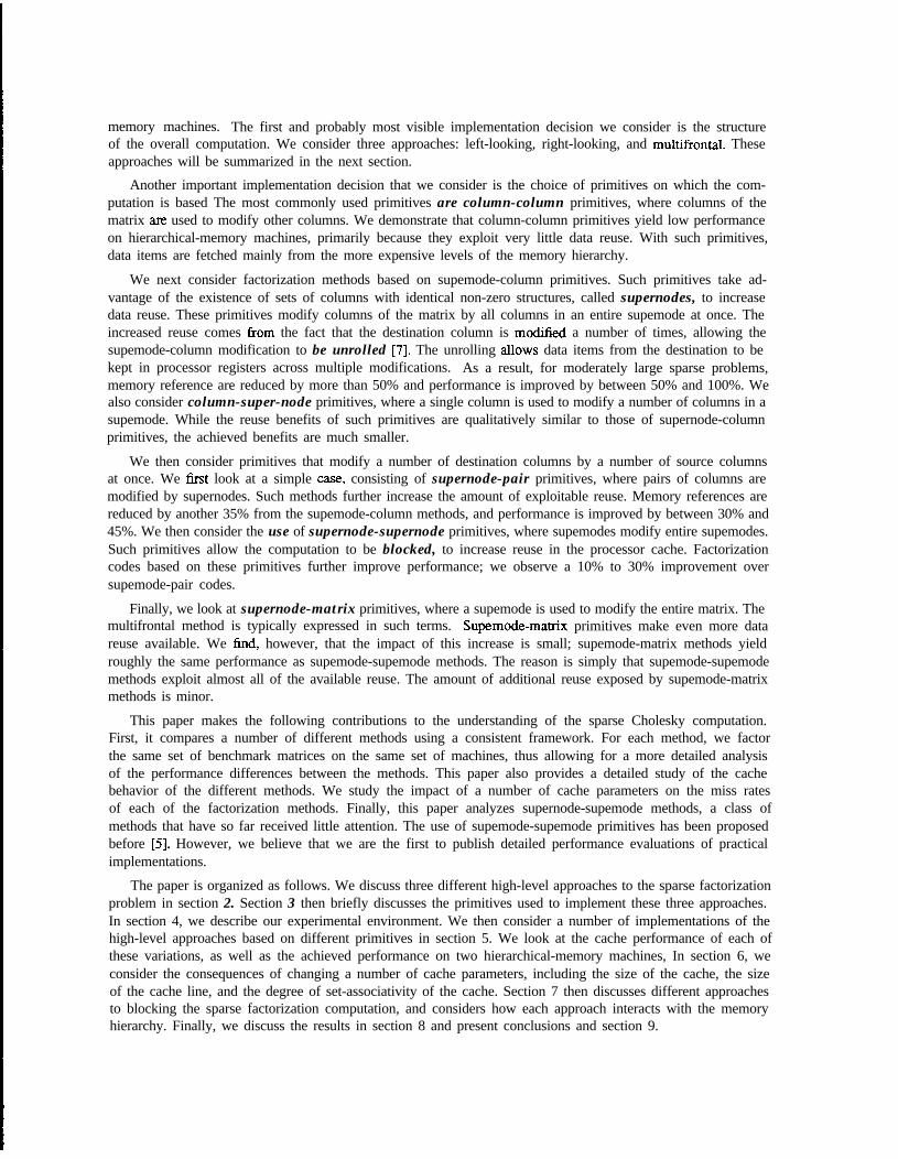
Figure 1: Non-zero structure of a matrix A and its factor L.

l \

l

’ 1l 2

3l 0 0 4

l 5

l l l a 6

Figure 2: Elimination tree of A.

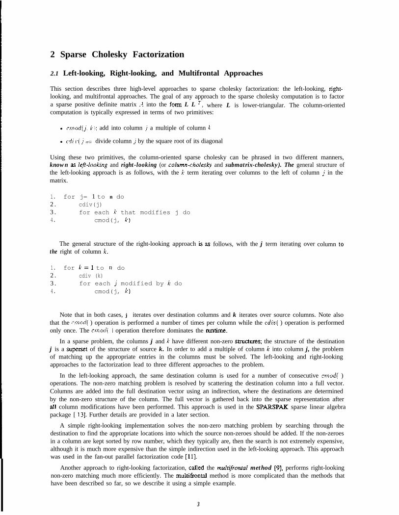
The multifrontal method is more easily explained in terms of the elimination tree [21] of the factor, astructure that we now describe. The elimination tree of a factor L is defined as

parent(j) = min{il/,, # 0. i > j}.

In other words, the parent of column j is determined by the first sub-diagonal non-zero in column j. Equivalently,the parent of column j is the Crst column modified by column j. As an example, in Figure 1 we have a matrix-4, and its factor L. In Figure 2 we show the elimination tree of this matrix. The elimination tree providesa great deal of information about the structure of the sparse cholesky computation. One important piece ofinformation that can be obtained from the elimination tree is the set of columns that can possibly be modifiedby a column. A column can only modify its ancestors in the elimination tree. Equivalently, a column can onlybe modified by its descendents.

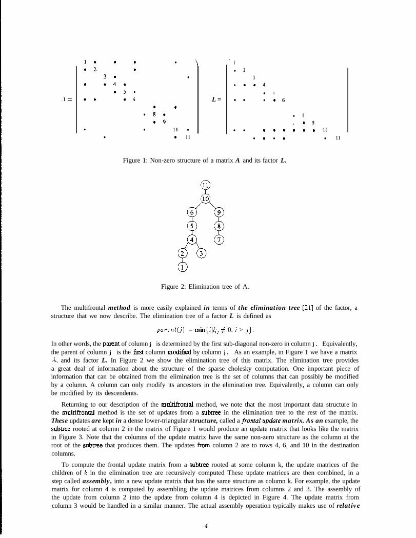
Returning to our description of the multifrontal method, we note that the most important data structure inthe multiontal method is the set of updates from a subtree in the elimination tree to the rest of the matrix.These updates are kept in a dense lower-triangular structure, called a frontaZ update matrix. As an example, thesubtree rooted at column 2 in the matrix of Figure 1 would produce an update matrix that looks like the matrixin Figure 3. Note that the columns of the update matrix have the same non-zero structure as the column at theroot of the subtree that produces them. The updates Tom column 2 are to rows 4, 6, and 10 in the destinationcolumns.

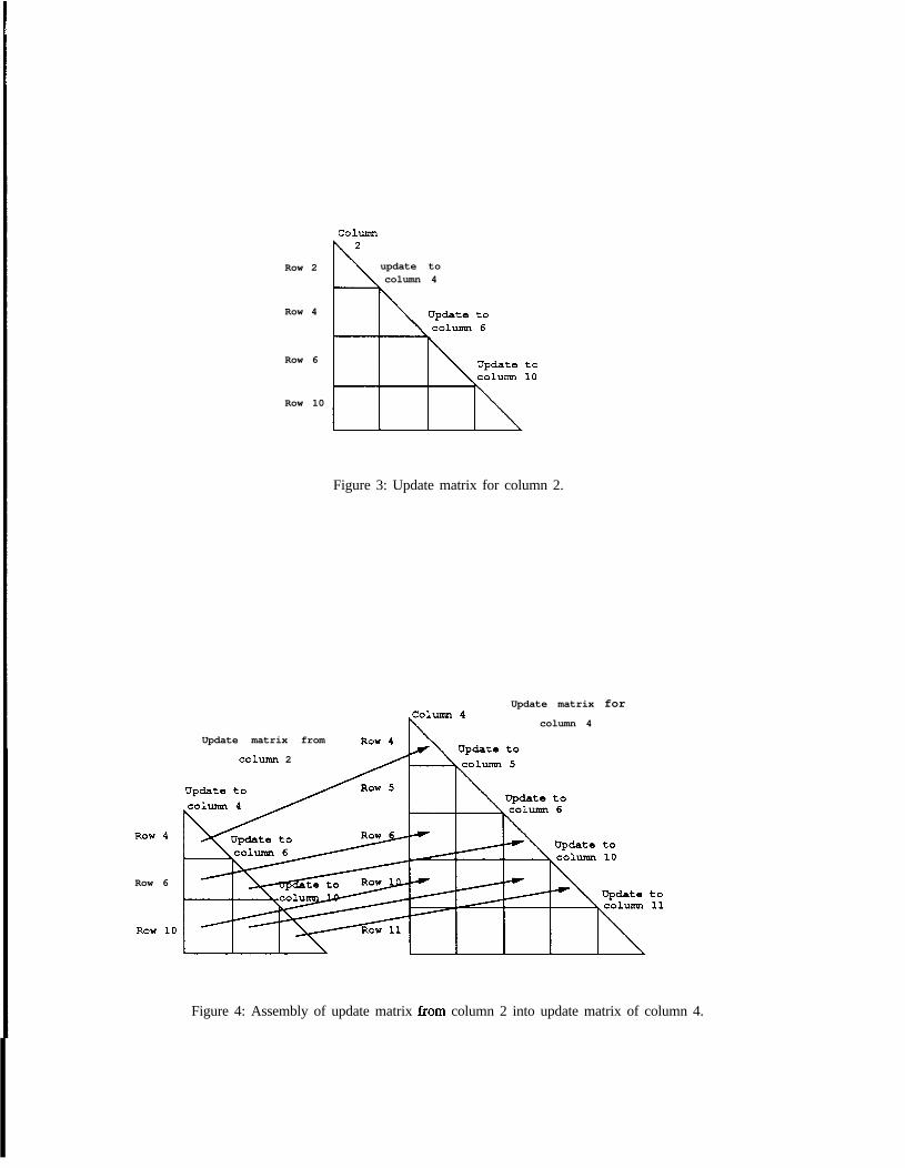
To compute the frontal update matrix from a subtree rooted at some column k, the update matrices of thechildren of k in the elimination tree are recursively computed These update matrices are then combined, in astep called assembly, into a new update matrix that has the same structure as column k. For example, the updatematrix for column 4 is computed by assembling the update matrices from columns 2 and 3. The assembly ofthe update from column 2 into the update from column 4 is depicted in Figure 4. The update matrix fromcolumn 3 would be handled in a similar manner. The actual assembly operation typically makes use of relative

4

Column

Row 6

2

Row 2 n update tocolumn 4

Row 4

Row 6

Row 10

Figure 3: Update matrix for column 2.

Update matrix from

colum 2

Update matrix for

column 4

Figure 4: Assembly of update matrix from column 2 into update matrix of column 4.

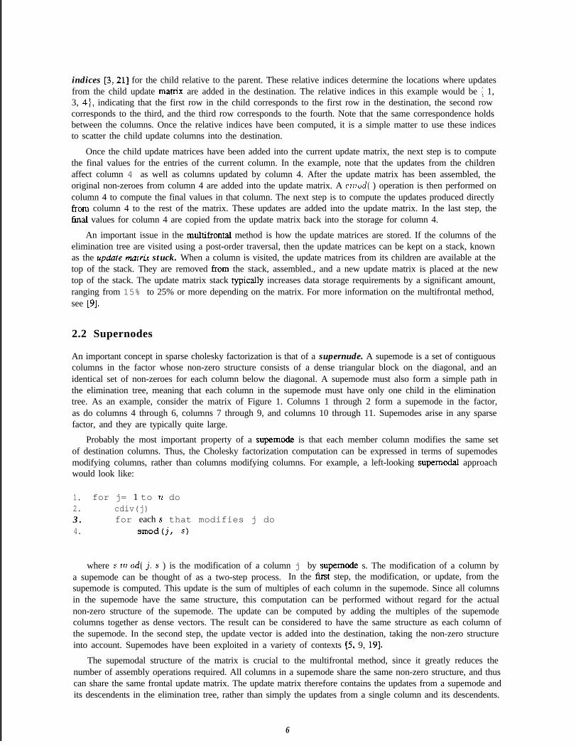
indices [3, 211 for the child relative to the parent. These relative indices determine the locations where updatesfrom the child update matrix are added in the destination. The relative indices in this example would be { 1,3, 4}, indicating that the first row in the child corresponds to the first row in the destination, the second rowcorresponds to the third, and the third row corresponds to the fourth. Note that the same correspondence holdsbetween the columns. Once the relative indices have been computed, it is a simple matter to use these indicesto scatter the child update columns into the destination.

Once the child update matrices have been added into the current update matrix, the next step is to computethe final values for the entries of the current column. In the example, note that the updates from the childrenaffect column 4 as well as columns updated by column 4. After the update matrix has been assembled, theoriginal non-zeroes from column 4 are added into the update matrix. A onod( ) operation is then performed oncolumn 4 to compute the final values in that column. The next step is to compute the updates produced directlyfrom column 4 to the rest of the matrix. These updates are added into the update matrix. In the last step, thefinal values for column 4 are copied from the update matrix back into the storage for column 4.

An important issue in the multifrontal method is how the update matrices are stored. If the columns of theelimination tree are visited using a post-order traversal, then the update matrices can be kept on a stack, knownas the update matrix stuck. When a column is visited, the update matrices from its children are available at thetop of the stack. They are removed from the stack, assembled., and a new update matrix is placed at the newtop of the stack. The update matrix stack typically increases data storage requirements by a significant amount,ranging from 15% to 25% or more depending on the matrix. For more information on the multifrontal method,see [9].

2.2 Supernodes

An important concept in sparse cholesky factorization is that of a supernude. A supemode is a set of contiguouscolumns in the factor whose non-zero structure consists of a dense triangular block on the diagonal, and anidentical set of non-zeroes for each column below the diagonal. A supemode must also form a simple path inthe elimination tree, meaning that each column in the supemode must have only one child in the eliminationtree. As an example, consider the matrix of Figure 1. Columns 1 through 2 form a supemode in the factor,as do columns 4 through 6, columns 7 through 9, and columns 10 through 11. Supemodes arise in any sparsefactor, and they are typically quite large.

Probably the most important property of a supernode is that each member column modifies the same setof destination columns. Thus, the Cholesky factorization computation can be expressed in terms of supemodesmodifying columns, rather than columns modifying columns. For example, a left-looking supernodal approachwould look like:

1. for j= 1 to n do2. cdiv(j)3 . for each s that modifies j do4. smod(j, s)

where s ?n od( j. s ) is the modification of a column j by supernode s. The modification of a column bya supemode can be thought of as a two-step process. In the first step, the modification, or update, from thesupemode is computed. This update is the sum of multiples of each column in the supemode. Since all columnsin the supemode have the same structure, this computation can be performed without regard for the actualnon-zero structure of the supemode. The update can be computed by adding the multiples of the supemodecolumns together as dense vectors. The result can be considered to have the same structure as each column ofthe supemode. In the second step, the update vector is added into the destination, taking the non-zero structureinto account. Supemodes have been exploited in a variety of contexts [5, 9, 191.

The supemodal structure of the matrix is crucial to the multifrontal method, since it greatly reduces thenumber of assembly operations required. All columns in a supemode share the same non-zero structure, and thuscan share the same frontal update matrix. The update matrix therefore contains the updates from a supemode andits descendents in the elimination tree, rather than simply the updates from a single column and its descendents.

6

Supemodes will be exploited for a variety of purposes in this paper.

2.3 Assorted Details

This paper considers the performance of a number of implementations of each of the three described high-levelapproaches. In order to make these performance numbers more easily interpretable, we now provide additionaldetails of our specific implementations. In particular, we provide details on our multifrontal implementation.

The implementation of the multifrontal method has a number of possible variations. One variation involvesthe particular post-order traversal that is used to order the columns. We choose the traversal order that minimizesnecessary update stack space, using the techniques of [16]. We do not include the time spent determining thisorder in the computation times presented in the paper.

Another possible source of variation in the multifrontal method is in the approach used to handle the updatematrix stack. We use an approach that differs slightly from the traditional one, in order to remove an obvioussource of inefficiency for hierarchical-memory machines. In order to add a new update matrix to the top ofthe stack, the multifrontal method must first consume a number of update matrices already there. A traditionalimplementation would compute the new update matrix at one location, remove the consumed updates matricesfrom the top of the stack, and then copy the completed update matrix to the new top of the stack. Such copyingis very expensive on a hierarchical-memory machine, so we introduce a simple trick to remove it. Rather thankeeping a single update matrix stack we keep two stacks that grow towards each other. Update matrices areconsumed from the top of one stack, and produced onto the top of the other stack. Another way of thinkingabout this trick is in terms of the depth of a supemode in the elimination tree. The update matrices fromsupemodes of odd depth are kept on one stack, with the update matrices from supemodes of even depth onthe other. This trick eliminates the necessity of copying update matrices. This approach is not without costs,however. We observed a 20-50% increase in the amount of stack space required. This modification introducesa tradeoff between the performance of the computation and the amount of space required to perform it. Weinvestigate the higher performance approach.

3 Sparse Cholesky Primitives

The three high-level approaches to sparse Cholesky factorization that have been described, the left-looking, right-looking, and multifrontal methods, have so far been expressed in terms of column-column or supemode-columnmodifications. In this paper, we consider a range of possible primitives for expressing the sparse Choleskycomputation. In terms of more general primitives, a left-looking Cholesky factorization computation would looklike:

1. for j= 1 to -TS do2. for each k that modifies j do3. ComputeUpdateToJFromK(j, k)4. PropagateUpdateToJFromK(j, k)5. Complete(j)

The C’omylete ( ) primitive computes the final values of the elements within a structure, once all modificationsfrom other structures have been performed. The C’omput cl’pdaf t ( ) primitive computes the update from onestructure to the other. The Propagat E I’pdate( ) primitive subsequently adds the computed update into theappropriate destination locations. In the case of the cmod( ) primitive, the computation and propagation of theupdate are performed as a single step. The .YS term in the above pseudo-code represents the number of differentdestination structures in the matrix. An important thing to note is that j and k do not necessarily iterate overthe same types of structures.

A generalized right-looking approach would look like:

1. for k= 1 to .Ys do2. Complete(k)

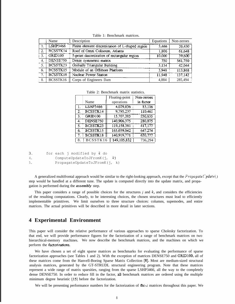
[Table 1: Benchmark matrices.

1 Name 11 Description 1 Equations 1 Non-zeroes

[ 8. BCSSTK16 Corps of Engineers Dam 4,884 1 285,494 1

Table 2: Benchmark matrix statistics.

I I /I Floating-pointName operations

1 8 . 1 BCSSTK16 11 149,105,832 1 736,294 1

3 .4.5.

for each j modified by k doComputeUpdateToJFromK(j, k)PropagateUpdateToJFromK(j, k)

A generalized multifrontal approach would be similar to the right-looking approach, except that the Propuyutrl’pdute( )step would be handled at a different tune. The update is computed directly into the update matrix, and propa-gation is performed during the assembly step.

This paper considers a range of possible choices for the structures j and k, and considers the efficienciesof the resulting computations. Clearly, to be interesting choices, the chosen structures must lead to efficientlyimplementable primitives. We limit ourselves to three structure choices: columns, supemodes, and entirematrices. The actual primitives will be described in more detail in later sections.

4 Experimental Environment

This paper will consider the relative performance of various approaches to sparse Cholesky factorization. Tothat end, we will provide performance figures for the factorization of a range of benchmark matrices on twohierarchical-memory machines. We now describe the benchmark matrices, and the machines on which weperform the factorizations.

We have chosen a set of eight sparse matrices as benchmarks for evaluating the performance of sparsefactorization approaches (see Tables 1 and 2). With the exception of matrices DENSE750 and GRIDlOO, all ofthese matrices come from the Hanvell-Boeing Sparse Matrix Collection [8]. Most are medium-sized structuralanalysis matrices, generated by the GT-STRUDL structural engineering program. Note that these matricesrepresent a wide range of matrix sparsities, ranging from the sparse LSHP3466, all the way to the completelydense DENSE750. In order to reduce fill in the factor, all benchmark matrices are ordered using the multipleminimum degree heuristic [15] before the factorization.

We will be presenting performance numbers for the factorization of the:,2 matrices throughout this paper. We

8

will typically present numbers for each matrix, as well as summary numbers. The summary numbers will takethree forms. One number will be the mean performance (harmonic mean) over all the benchmark matrices. Inorder to give some idea of how the methods perform on small and large problems, we will also present meansover subsets of the benchmark matrices. In particular, we call matrices LSHP3466, BCSSTK14, and GRID100smd matrices, and similarly we call BCSSTKLS, BCSSTK16, and BCSSTK18 large matrices. We do not meanto imply that the latter three matrices are large in an absolute sense. In fact, they are of quite moderate size bycurrent standards. We simply mean that they almost fill the main memories of the benchmark machines, andthus are the largest matrices in our benchmark set.

The two machines on which we perform the sparse factorization computations axe the DECstation 3100and the IBM RS/6000 Model 320. Both are high-performance RISC machines with memory hierarchies. TheDECstation 3100 uses a MIPS R2000 processor and an R2010 floating-point coprocessor, each operating at16MHz. It contains a 64-KByte data cache, a 64-KByte instruction cache, and 16 MBytes of main memory.The machine is nominally rated at 1.6 double-precision LINPACK MFLOPS. The IBM RS/6000 Model 320uses the IBM RS/6000 processor, operating at 20 MHz. The Model 320 contains 32 ISBytes of data cache,32 KBytes of instruction cache, and 16 MBytes of main memory. The Model 320 is nominally rated at 7.4double-precision LINPACK MFLOPS.

The data cache on the DECstation 3100 is direct-mapped, meaning that each location in memory maps toa specific line in the cache. If a location is fetched into the cache, then the fetched location displaces the datathat previously resided in that line. Two memory data items that map to the same line and frequently displaceeach other are said to interfere in the cache. The cache lines in the DECstation 3 100 are 4 bytes long.

The data cache on the IBM RS/6000 Model 320 is 4-way set-associative, meaning that each location inmemory maps to any of 4 different lines in the cache. Replacement in the cache is done on an LRU, orleast-recently-used basis, meaning that a fetched location displaces the least recently used of the data items thatreside in its four possible lines. Each cache line contains 64 bytes.

The relative costs of various operations on these machines are quite important in understanding their per-formance. On the DECstation 3100, a double-precision multiply requires 5 cycles, and a double-precision addrequires 2 cycles. Adds and multiplies can be overlapped in a limited manner. A single add can be performedwhile a multiply is going on, but an add cannot be overlapped with another add, and similarly a multiply can-not be overlapped with another multiply. The peak floating-point performance of the machine is therefore onemultiply-add combination every 5 cycles. A cache miss requires roughly 6 cycles to service. A double-precisionnumber spans two cache lines, thus requiring double the cache miss time to fetch. On the IBM RS/6000 Model320, adds and multiplies each require two cycles to complete. However, the floating-point unit is fully pipelined,meaning that adds and multiplies can be overlapped in any possible way. In particular, a floating-point instruc-tion can be initiated every cycle. Furthermore, the machine contains a multiply-add instruction that performsboth instructions in the same time it would take to perform either individual operation. The RS/6000 can issueup to four different instructions in a single cycle. The peak floating-point performance of the IBM RS/6000 is

cycle. A 15 cycles to service, bringing inone multiply-add pera 64-byte cache line.

cache miss on the Model 320 requires roughly

From these performance numbers, it is clear that memory system costs are an extremely important componentof the runtime of a matrix computation. The cost of performing floating-point arithmetic is dwarfed by the costof moving data between the various levels of the memory hierarchy. As a simple example, the RS/6000requires more instructions to load three operands from the cache to processor registers than it does to performa double-precision multiply-add operation on them. The cost of loading them from main memory is muchhigher. For this reason, the performance of a linear algebra program in general depends more on the memorysystem demands of the program than on the number of floating-point operations performed. Our analysis offactorization performance will concentrate on the memory system behavior of the various approaches.

‘To provide concrete numbers for comparing the memory system behaviors of the various factorizationmethods, we will present counts of the number of memory references and the number of cache misses a methodgenerates in factoring a matrix. These numbers are gathered using the Tango simulation environment [6]. Tangois used to instrument the factorization programs to produce a trace of all data references the programs generate.We count these references to produce memory reference counts and feed them into a cache simulator to producecache miss counts.

Another factor that will be important in understanding the performance of the IBM RS/6000 is the amount

9

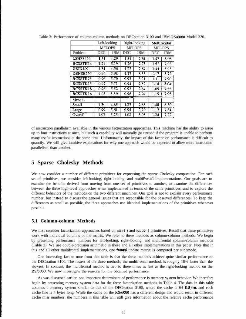
Table 3: Performance of column-column methods on DECstation 3100 and IBM RS/6000 Model 320.Left-looking Right-looking MultifYontal

MFLOPS MFLOPS MFLOPSProblem DEC ) IBM DEC 1 IBM DEC 1 IBM

of instruction parallelism available in the various factorization approaches. This machine has the ability to issueup to four instructions at once, but such a capability will naturally go unused if the program is unable to performmany useful instructions at the same time. Unfortunately, the impact of this factor on performance is difficult toquantify. We will give intuitive explanations for why one approach would be expected to allow more instructionparallelism than another.

5 Sparse Cholesky Methods

We now consider a number of different primitives for expressing the sparse Cholesky computation. For eachset of primitives, we consider left-looking, right-looking, and mu.ltif?ontal implementations. Our goals are toexamine the benefits derived from moving from one set of primitives to another, to examine the differencesbetween the three high-level approaches when implemented in terms of the same primitives, and to explore thedifferent behaviors of the methods on the two different machines. Our goal is not to explain every performancenumber, but instead to discuss the general issues that are responsible for the observed differences. To keep thedifferences as small as possible, the three approaches use identical implementations of the primitives wheneverpossible.

5.1 Column-column Methods

We first consider factorization approaches based on cdi t*( ) and cmod( ) primitives. Recall that these primitiveswork with individual columns of the matrix. We refer to these methods as column-column methods. We beginby presenting performance numbers for left-looking, right-looking, and multifrontal column-column methods(Table 3). We use double-precision arithmetic in these and all other implementations in this paper. Note that inthis and all other multifrontal implementations, one frontal update matrix is computed per supemode.

One interesting fact to note from this table is that the three methods achieve quite similar performance onthe DECstation 3100. The fastest of the three methods, the multifrontal method, is roughly 16% faster than theslowest. In contrast, the multifrontal method is two to three times as fast as the right-looking method on theRS/6000. We now investigate the reasons for the obtained performance.

As was discussed earlier, one important determinant of performance is memory system behavior. We thereforebegin by presenting memory system data for the three factorization methods in Table 4. The data in this tableassumes a memory system similar to that of the DECstation 3100, where the cache is 64 KBytes and eachcache line is 4 bytes long. While the cache on the RS/6000 has a different design and would result in differentcache miss numbers, the numbers in this table will still give information about the relative cache performance

10

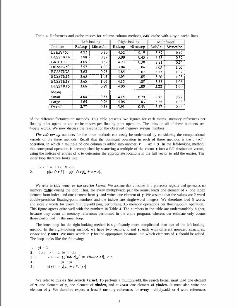
Table 4: References and cache misses for column-column methods, 64K cache with 4-byte cache lines.Left-looking Right-looking Multifrontal

Problem Refs/op 1 Misses/op Refs/op ) Misses/op Refs/op I Misses/op

of the different factorization methods. This table presents two figures for each matrix, memory references perfloating-point operation and cache misses per floating-point operation. The units on all of these numbers are4-byte words. We now discuss the reasons for the observed memory system numbers.

The refs-per-op numbers for the three methods can easily be understood by considering the computationalkernels of the three methods. Recall that the dominant operation in each of these methods is the cmod()operation, in which a multiple of one column is added into another, y - ax + y. In the left-looking method,this conceptual operation is accomplished by scattering a multiple of the vector x into a full destination vector,using the indices of entries of x to determine the appropriate locations in the full vector to add the entries. Theinner loop therefore looks like:

1 . for i= 1 to n do2. y[index[i]] = y[index[i]] + u * x[i]

We refer to this kernel as the scatter kernel. We assume that u resides in a processor register and generates nomemory traffic during the loop. Thus, for every multiply/add pair the kernel loads one element of x, one indexelement from index, and one element from y, and writes one element of y. We assume that the values are 2-worddouble-precision floating-point numbers and the indices are single-word integers. We therefore load 5 wordsand store 2 words for every multiply/add pair, performing 3.5 memory operations per floating-point operation.This figure agrees quite well with the numbers in Table 4. The numbers in the table are understandably higher,because they count all memory references performed in the entire program, whereas our estimate only countsthose performed in the inner loop.

The inner loop for the right-looking method is significantly more complicated than that of the left-lookingmethod. In the right-looking method, we have two vectors, x and y, each with different non-zero structures,xindex and yindex. We must search in y for the appropriate locations into which elements of x should be added.The loop looks like the following:

1. yi = 12. for xi=1 to n do3 : w h i l e (yindex[yi] # xindex[xi]) d o4. yi = yi + 15. y[yi] = y[yi] + a * x[ci]

We refer to this as the search kernel. To perform a multiply/add, the search kernel must load one elementof x, one element of y, one element of xindex, and at least one element of yindex. It must also write oneelement of y. We therefore expect at least 8 memory references for every multiply/add, or 4 word references

11

for every floating-point operation. The numbers in the table are often less than this figure because of a specialcase in the right-looking method. One can easily determine whether the source and destination vectors have thesame length. Since the structure of the destination is a superset of the structure of the source, the two vectorsnecessarily have the same structure if they have the same length. The index vectors can then be ignored entirelyand the vectors can be added together directly.

The multifrontal method has a much simpler kernel than either of the previous two methods. Recall that themultifrontal method adds a column of the matrix into an update column, and the update column has the samenon-zero structure as the updating column. Thus the computational kernel is a simple DAXPY:

1. for i = 1 to I) do2 . y[i] = y[i] $ a * x[i]

This kernel loads 4 words and writes 2 words for every iteration, for a ratio of 3 memory operations perfloating point operation. The multifrontal method must also combine, or assemble, update matrices to formsubsequent update matrices. The memory references performed during assembly are responsible for the fact thatthe numbers in the table are larger than would be predicted by the kernel.

The cache miss rates for the three methods can be understood by considering the following. In each method,some column is used repetitively. In the left-looking method, the destination column is modified by a numberof columns to its left, while in the right-looking and multifrontal methods, the source column modifies a numberof columns to its right. Thus, in each of the three y - ax + y kernels from above, one of the two vectors x ory does not change from one invocation to the next. With a reasonably large cache, we would expect this vectorto remain in the cache, thus we would only expect one vector to miss per column modification. In other words,for every multiply/add, we would expect to cache miss on one double-precision vector element, yielding a missrate of one word per floating-point operation.

The index vectors may appear to cause significant misses as well, but recall that adjacent columns frequentlyhave the same non-zero structures. These columns share the same index vector in the sparse matrix representation.Thus, even when the miss rate on the non-zeroes is high, the miss rate on the index structures is typically quitelow.

The performance of the three method on the DECstation 3100 can be easily understood in terms of thismemory system data. A substantial portion (roughly 35% for the larger matrices) of the runtirne goes to servicingcache misses. Since the three methods generate roughly the same number of cache misses, this cost is the samefor alI three. The performance differences between the methods are due primarily to the differences in thenumber of memory references.

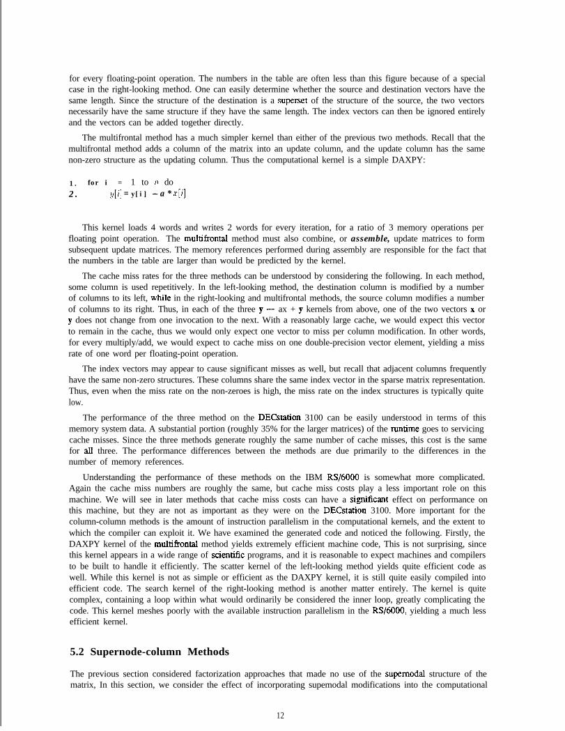
Understanding the performance of these methods on the IBM RS/6000 is somewhat more complicated.Again the cache miss numbers are roughly the same, but cache miss costs play a less important role on thismachine. We will see in later methods that cache miss costs can have a sign&ant effect on performance onthis machine, but they are not as important as they were on the DECstation 3100. More important for thecolumn-column methods is the amount of instruction parallelism in the computational kernels, and the extent towhich the compiler can exploit it. We have examined the generated code and noticed the following. Firstly, theDAXPY kernel of the multifrontal method yields extremely efficient machine code, This is not surprising, sincethis kernel appears in a wide range of scientic programs, and it is reasonable to expect machines and compilersto be built to handle it efficiently. The scatter kernel of the left-looking method yields quite efficient code aswell. While this kernel is not as simple or efficient as the DAXPY kernel, it is still quite easily compiled intoefficient code. The search kernel of the right-looking method is another matter entirely. The kernel is quitecomplex, containing a loop within what would ordinarily be considered the inner loop, greatly complicating thecode. This kernel meshes poorly with the available instruction parallelism in the RS/6000, yielding a much lessefficient kernel.

5.2 Supernode-column Methods

The previous section considered factorization approaches that made no use of the supernodal structure of thematrix, In this section, we consider the effect of incorporating supemodal modifications into the computational

12

kernel, where the update from an entire supemode is formed using dense matrix operations, and then theaggregate update is added into its destination. Supemodal elimination can be easily integrated into each of theapproaches of the previous section [5].

We now consider the implementation of supemode-column primitives. RecaIl that our generalized phras-ing of the factorization computation identifies three primitives: C’nmpclteIITpdufc( ), P~‘ol)c~yclt~l-l,dc~~( ), andC-‘o?~)])IE tf ( ). For a particular set of primitives, the same C’omy~tel-lxlufe( ) can be used for the left-looking,right-looking and multifrontal approaches. The Propgut~I*pdute( ) primitive will differ among the three.

We begin by briefly describing the implementation of the update propagation step. Recall that this stepbegins once the update from a supemode to a column has been computed. The update has the same structureas the source supemode. In the supemode-column left-looking method, the update is scattered into the fulldestination vector, using the structure of the source supernode to determine the appropriate positions. Noticethat this operation is nearly identical to the scatter kernel of the column-column method. In the right-lookingsupemode-column method, the update is added into the appropriate positions in the destination column using asearch. Again, this operations is nearly identical to the corresponding column-column kernel. In the multifrontalsupemode-column method., the update is computed directly into the frontal update matrix, so no propagation isimmediately necessary. Although the supemode-column propagation primitives are quite similar to the corre-sponding modification kernels of the column-column methods, this do not imply that the overall performance ofthe two approaches will be similar. The propagation primitives in the supemode-column methods occur muchless frequently than the modification kernels in the column-column methods, so they have a much smaller impacton performance.

We now turn our attention to the C’o,,?I’utel-IJdut~() step, a step that is common among the three methods.In fact, to make the three methods more directly comparable, we use the identical code for each. Recall thatthe update from a supemode to a column is computed using a dense rank-k update, where the I< vectors usedin the update are the columns of the source supemode, below the diagonal of the destination. The basic kernelappears as follows:

1. for k= 1 to I< do2. for i= 1 to n do3. y[i] = y[i] + uk * xk[i]

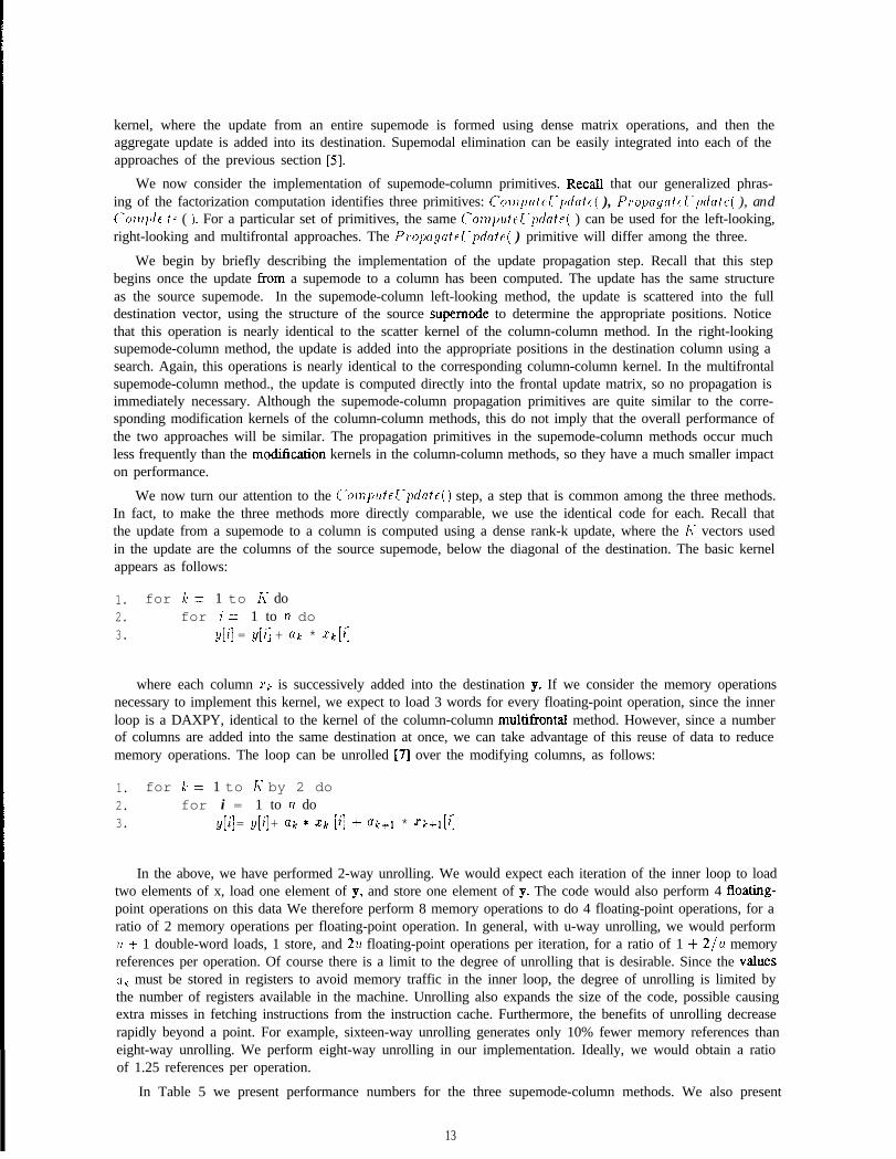
where each column .rk is successively added into the destination y. If we consider the memory operationsnecessary to implement this kernel, we expect to load 3 words for every floating-point operation, since the innerloop is a DAXPY, identical to the kernel of the column-column multifrontal method. However, since a numberof columns are added into the same destination at once, we can take advantage of this reuse of data to reducememory operations. The loop can be unrolled [7] over the modifying columns, as follows:

1. for k= 1 to I< by 2 do2. for i = 1 to n do3. y[i] = y[i] + ak * xk [i] + uk+l * Xk+l[i]

In the above, we have performed 2-way unrolling. We would expect each iteration of the inner loop to loadtwo elements of x, load one element of y, and store one element of y. The code would also perform 4 floating-point operations on this data We therefore perform 8 memory operations to do 4 floating-point operations, for aratio of 2 memory operations per floating-point operation. In general, with u-way unrolling, we would performII i 1 double-word loads, 1 store, and 2[1 floating-point operations per iteration, for a ratio of 1 + 2/u memoryreferences per operation. Of course there is a limit to the degree of unrolling that is desirable. Since the valueselk must be stored in registers to avoid memory traffic in the inner loop, the degree of unrolling is limited bythe number of registers available in the machine. Unrolling also expands the size of the code, possible causingextra misses in fetching instructions from the instruction cache. Furthermore, the benefits of unrolling decreaserapidly beyond a point. For example, sixteen-way unrolling generates only 10% fewer memory references thaneight-way unrolling. We perform eight-way unrolling in our implementation. Ideally, we would obtain a ratioof 1.25 references per operation.

In Table 5 we present performance numbers for the three supemode-column methods. We also present

13

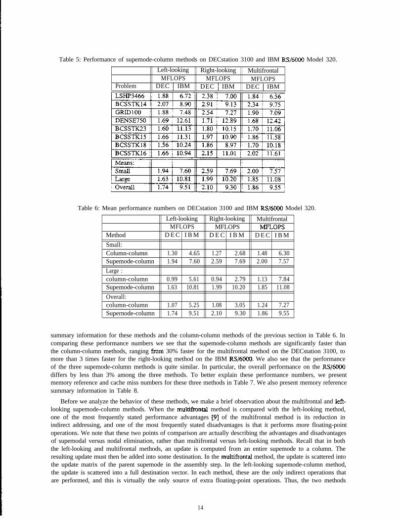
Table 5: Performance of supemode-column methods on DECstation 3100 and IBM RS/6000 Model 320.

Left-looking Right-looking MultifrontalMFLOPS MFLOPS MFLOPS

Problem DEC 1 IBM DEC 1 IBM DEC 1 IBM

Table 6: Mean performance numbers on DECstation 3100 and IBM RS/6000 Model 320.

Left-looking Right-looking MultifrontalMFLOPS MFLOPS MFLOPS

Method D E C I B M D E C I B M D E C I B MSmall:Column-column 1.30 4.65 1.27 2.68 1.48 6.30Supemode-column 1.94 7.60 2.59 7.69 2.00 7.57Large :column-column 0.99 5.61 0.94 2.79 1.13 7.84Supemode-column 1.63 10.81 1.99 10.20 1.85 11.08Overall:column-column 1.07 5.25 1.08 3.05 1.24 7.27Supernode-column 1.74 9.51 2.10 9.30 1.86 9.55

summary information for these methods and the column-column methods of the previous section in Table 6. Incomparing these performance numbers we see that the supemode-column methods are significantly faster thanthe column-column methods, ranging from 30% faster for the multifrontal method on the DECstation 3100, tomore than 3 times faster for the right-looking method on the IBM RS/6000. We also see that the performanceof the three supemode-column methods is quite similar. In particular, the overall performance on the RS/6000differs by less than 3% among the three methods. To better explain these performance numbers, we presentmemory reference and cache miss numbers for these three methods in Table 7. We also present memory referencesummary information in Table 8.

Before we analyze the behavior of these methods, we make a brief observation about the multifrontal and left-looking supemode-column methods. When the multifrontal method is compared with the left-looking method,one of the most frequently stated performance advantages [9] of the multifrontal method is its reduction inindirect addressing, and one of the most frequently stated disadvantages is that it performs more floating-pointoperations. We note that these two points of comparison are actually describing the advantages and disadvantagesof supemodal versus nodal elimination, rather than multifrontal versus left-looking methods. Recall that in boththe left-looking and multifrontal methods, an update is computed from an entire supemode to a column. Theresulting update must then be added into some destination. In the multifrontal method, the update is scattered intothe update matrix of the parent supemode in the assembly step. In the left-looking supemode-column method,the update is scattered into a full destination vector. In each method, these are the only indirect operations thatare performed, and this is virtually the only source of extra floating-point operations. Thus, the two methods

14

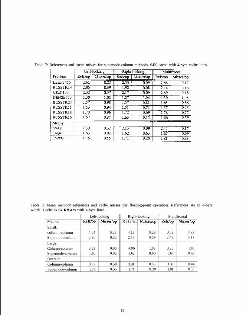
Table 7: References and cache misses for supemode-column methods, 64K cache with 4-byte cache lines.

Table 8: Mean memory references and cache misses per floating-point operation. References are to 4-bytewords. Cache is 64 KBytes with 4-byte lines.

Left-looking Right-looking MultifrontalMethod Refs/op Misses/op Refs /op M.isses/op Refs/op Mkes/opSmall:column-column 4.04 0.35 4.18 0.29 3.72 0.22Supemodecolumn 2.30 0.32 2.13 0.09 2.45 0.17Large:Column-column 3.65 0.96 4.06 1.03 3.25 1.03Supemode-column 1.63 0.92 1.62 0.63 1.67 0.69Overall:Column-column 3.77 0.58 3.91 0.53 3.37 0.44Supemode-column 1.76 0.55 1.71 0.20 1.81 0.33

15

are almost entirely equivalent in terms of indirect operations and extra floating-point operations.

Returning to the memory reference numbers, it is somewhat surprising to note that even though the multi-frontal and left-looking methods exhibit roughly equivalent behavior, the two methods do not produce the samenumber of memory references. The differences are much smaller than they were in the column-column methods,because the methods share the same kernel, but differences still exist. The difference is caused by additional datamovement in the mu.ltif?ontal method, due to two subtle differences between the methods. The first differenceis related to the destinations into which updates are added. In the left-looking method (and the right-lookingmethod as well), updates are always added directly into the destination column. In the m&frontal method,updates are added into update matrices. When all updates to a column have been performed the left-lookingand right-looking methods complete that column in-place. The multifrontal method, on the other hand, adds theoriginal column entries into the update matrix, computes the final values of that column, and then copies thefinal values back to the column storage.

The other difference relates to the manner in which supemodes containing a single column are handled. Theprocess of producing an update matrix for a single column and then propagating it is significantly less efficientthan the process used in, for example, the column-column left-looking method, where the update is computedand propagated in the same step. In the left-looking and right-looking methods, we can fall back to the column-column kernels for supemodes containing only a single column. This option does not exist for the multifrontalmethod. We find through simulation that the lack of a single-column special case accounts for slightly morethan half of the increase in memory references, with the movement of completed columns accounting for therest. We also find that the relative cost of this additional data movement is larger for smaller problems. This isto be expected, for two reasons. First, the number of operations done in a sparse factorization grows much morequickly than the number of non-zeroes in the factor. Thus, the relative cost of moving each factor non-zeroto and from an update matrix decreases as the problem size increases. The other reason is that single-columnsupemodes generally account for a much smaller portion of the total operations in larger problems. In summary,the multifrontal method has a performance disadvantage when compared to the left-looking and right-lookingmethods because it performs additional data movement.

Returning to the memory reference numbers, another thing to note is that the numbers for the supemode-column methods are significantly lower than those for the column-column methods (see Table 8). Depending onthe problem and the method, the number of references has decreased to between 45% and 55% of their previouslevels. This decrease is due to two factors. First, the supemode-column methods access index vectors much lessfrequently. Second, the supernodal methods achieve improved reuse of processor registers due to loop unrolling.For the left-looking method, we find that the reduced index vector accesses bring references down to roughly90% of their previous levels. The loop unrolling accounts for the rest of the decrease.

Something else to note is that the references per operation numbers are well above the 1.25 ideal number.The reason is simply that not all supemodes are large enough to take full advantage of the reuse benefits ofsupemodal elimination.

Regarding the cache performance of the three methods, we also notice an interesting change. The cachemiss numbers for the left-looking method have remained virtually unchanged between the column-column andsupemode-column variants. The numbers for the right-looking and multifrontal methods, on the other hand,have decreased significantly. This fact can be understood by considering where reuse occurs in the cache. In theleft-looking column-column method, the data that is reused is the destination column. In the supemode-columnleft-looking method, this reuse has not changed. We expect that the destination column to remain in the cache,and the supemodes that update it to miss in the cache, again resulting in a miss rate of approximately one wordper floating-point operation.

In the right-looking and multifrontal methods, updates are now produced from a supemode to a numberof columns. Thus, the item that is reused is a supemode. We see three possibilities for the behavior of thecache, depending on the size of the supemode. If the supemode contains a single column, then we wouldexpect the supemode to remain in the cache, and the destination columns to cache miss, resulting in one missper floating-point operation. If the supemode contains more than one column but is smaller than the cache,then we would again expect the supemode to remain in the cache, and the destination to miss. However, weare now performing many more floating-point operations on each entry in the destination. In particular, if ccolumns remain in the cache, then we perform c times as many operations per cache miss. If the supemode ismuch larger than the processor cache, then we expect the destination to remain in the processor cache while

16

the supemode update is being computed, as would happen in the left-looking method, resulting in one miss perfloating-point operation. The cache miss numbers in Table 7 indicate that the case where a supemode fits in thecache occurs quite frequently, resulting in significantly fewer misses than one miss per floating-point operationoverall.

Another interesting item to note in the cache miss numbers is the difference between the miss rates of themultifrontal and right-looking methods. It would appear that since both methods take a right-looking approachto the factorization, they should have identical cache miss behaviors. The reason that they do not is that themultifrontal method performs more data movement. We discussed earlier the reasons why the multifrontalmethod performed more data movement than the left-looking method. The same reasons hold true when themultifrontal method is compared to the right-looking method. Simulation has shown that slightly more than halfof the extra memory references are due to the methods used to handle single-column supemodes. In the caseof cache misses, simulation has shown that most of the extra misses are due to the copying of supemode datato and from update matrices.

Returning to the performance numbers (Table 5), we note that the right-looking method is now the fasteston the DECstation 3100, and the left-looking method is the slowest. The primary cause of the performancedifferences is the cache behavior of the various methods. The right-looking method generates the fewest misses,and is therefore the fastest. Similarly, the left-looking method generates the most and is the slowest. On theRS/6000, the left-looking and right-looking methods execute at roughly the same rate. While the right-lookingmethod has the advantage of generating fewer cache misses, it has the disadvantage of the inefficient propagationprimitive.

5.3 Column-supernode Methods

The supemode-column primitives of the previous section took advantage of the fact that a single destination isreused a number of times in a supemode-column update operation to increase reuse in the processor registers.They also took advantage of the fact that every column in the source supemode had the same non-zero structureto reduce the number of accesses to index vectors. A symmetric set of primitives, where a single column isused to modify an entire supemode, would appear to have similar advantages. We briefly show in this sectionthat while the advantages are qualitatively similar, they are not of the same magnitude.

Consider the implementation of a column-supemode Computel-ljdute( ) primitive. A column would beused to modify a set of destinations, appearing something like:

1. for j= 1 to .I do2. for i= 1 to n do3. y., [i] = y, [i] + a, * x[i]

Unrolling the j loop by a factor of two yields:

1. for j= 1 to J by 2 do2. for i= 1 to n do3. Yj [i] = Yj [i] + Clj * X[i]4. Y.~+i[il = Y~+i[i] + Uj+l * 44

The inner loop loads two entries of y, one entry of x, and stores two entries of y, for a total of 5 double-word references to perform 4 floating-point operations. In general, if we unroll II ways we load 11 entries ofy, one entry of x, and write 11 entries of y to perform 2 (1 floating-point operations, for a ratio of 2 + l/ 11memory references per floating-point operation. This ratio is still more than two-thirds of the ratio obtainedwithout unrolling, and double the ratio obtained by unrolling the supemode-column primitive. Thus, whilecolumn-supemode primitives realize some advantages due to reuse of data, they are not nearly as effective assupemode-column primitives. We therefore do not further study such methods.

17

5.4 Supernode-pair Methods

In this section, we consider a simple modification of the three supemode-column factorization methods thatfurther improves the efficiency of the computational kernels and also reduces the cache miss rates. The modifi-cation involves a change in the number of destination columns for the supemode modification primitives. Ratherthan modifying one column by a supemode, we now modify two. We call the resulting methods supernode-pair method. We will study a more general form of this modification, where a supemode modifies an entiresupemode, in the next subsection.

Devising factorization methods that make use of supemode-pair primitives is quite straightforward. Forall three approaches, the C-‘~H?~NI~F I-IK?u~~( ) primitive involves a pair of simultaneous rank-k updates, usingthe same vectors for each update. To handle update propagation in a left-looking method, we maintain twofull vectors, one for each destination column, and use the supemode-column left-looking propagation primitiveto update each. The bookkeeping necessary to determine which supemodes modify both current destinations,and which modify only one or the other is not difficult. The right-looking and multifrontal methods are alsoquite easily modified. In the both, we simply generate the updates to two destination columns at once. In theright-looking method, the two updates are propagated individually using the supemode-column right-lookingpropagation primitive.

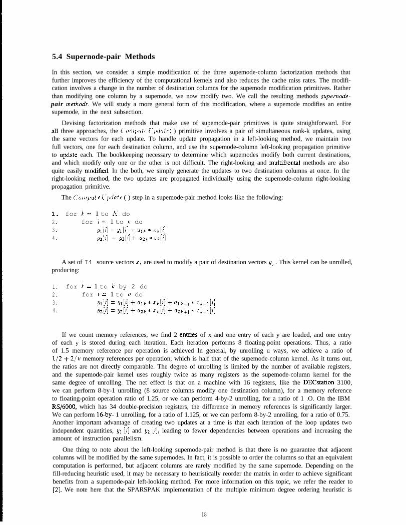
The C-‘~U~!JU~ E I’ljdafe ( ) step in a supemode-pair method looks like the following:

1. for k= 1 to I< do2. for i= 1 to n do3. Yl[i] = Yl[i] + Ulk * Xk[i]4. y2[i] = y*[i] + U2k * Xk[i]

A set of Ii source vectors .ck are used to modify a pair of destination vectors y, . This kernel can be unrolled,producing:

1. for k= 1 to k by 2 do2. for i= 1 to n do3. Yl[i] = Yl[i] i- Qlk * Q[i] + Qlb+1 * Q+l[j]4. Y2[i] = Y2[i] + Q2k * Xk[il + a2k+l * si-+1[il

If we count memory references, we find 2 enties of x and one entry of each y are loaded, and one entryof each y is stored during each iteration. Each iteration performs 8 floating-point operations. Thus, a ratioof 1.5 memory reference per operation is achieved In general, by unrolling u ways, we achieve a ratio ofl/2 + 2/u memory references per operation, which is half that of the supemode-column kernel. As it turns out,the ratios are not directly comparable. The degree of unrolling is limited by the number of available registers,and the supemode-pair kernel uses roughly twice as many registers as the supemode-column kernel for thesame degree of unrolling. The net effect is that on a machine with 16 registers, like the DECstation 3100,we can perform 8-by-1 unrolling (8 source columns modify one destination column), for a memory referenceto floating-point operation ratio of 1.25, or we can perform 4-by-2 unrolling, for a ratio of 1 .O. On the IBMRS/6000, which has 34 double-precision registers, the difference in memory references is significantly larger.We can perform 16by- 1 unrolling, for a ratio of 1.125, or we can perform 8-by-2 unrolling, for a ratio of 0.75.Another important advantage of creating two updates at a time is that each iteration of the loop updates twoindependent quantities, .~1 [i] and y2 [;I, leading to fewer dependencies between operations and increasing theamount of instruction parallelism.

One thing to note about the left-looking supemode-pair method is that there is no guarantee that adjacentcolumns will be modified by the same supernodes. In fact, it is possible to order the columns so that an equivalentcomputation is performed, but adjacent columns are rarely modified by the same supemode. Depending on thefill-reducing heuristic used, it may be necessary to heuristically reorder the matrix in order to achieve significantbenefits from a supemode-pair left-looking method. For more information on this topic, we refer the reader to[2]. We note here that the SPARSPAK implementation of the multiple minimum degree ordering heuristic is

18

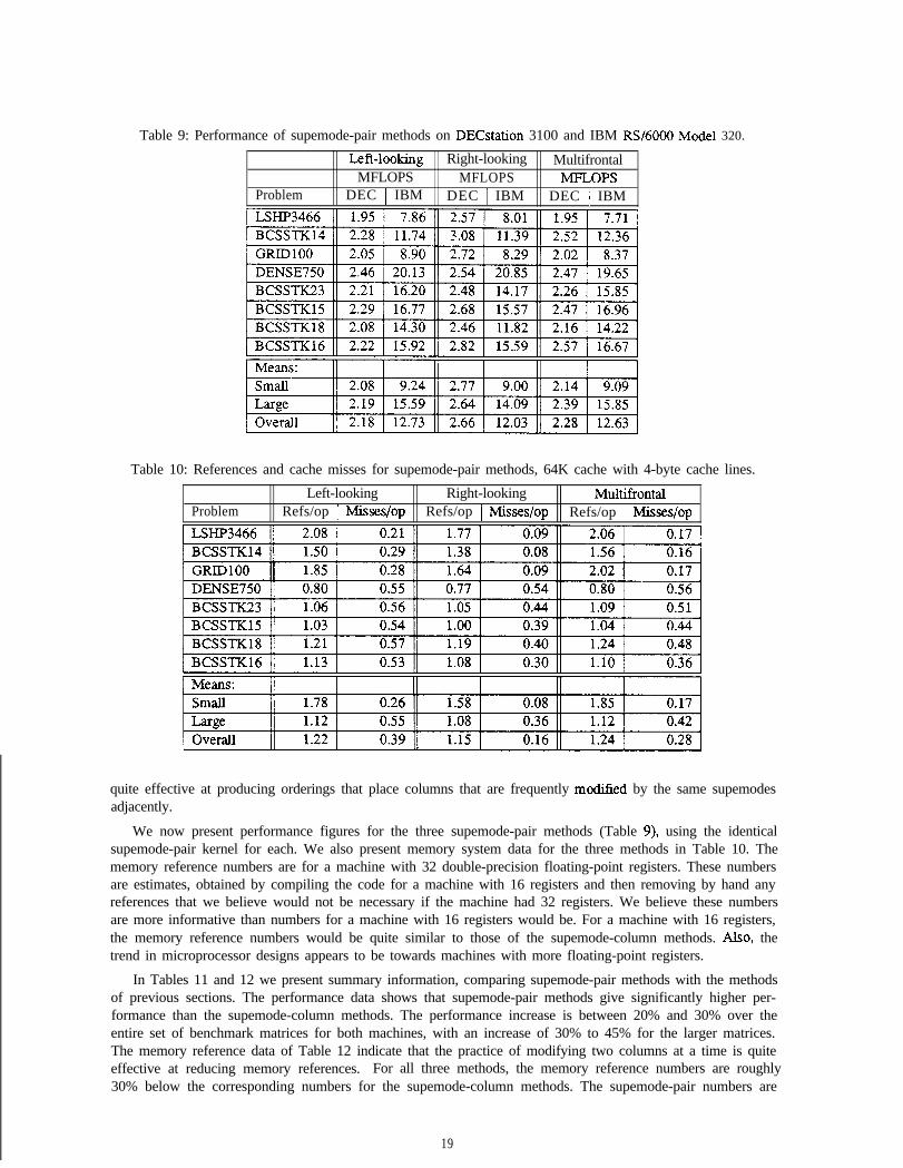
Table 9: Performance of supemode-pair methods on DECstation 3100 and IBM RS/6000 Model 320.

Left-lool&Ag Right-looking MultifrontalMFLOPS MFLOPS MFLOPS

Problem DEC 1 IBM DEC 1 IBM DEC 1 IBM

Table 10: References and cache misses for supemode-pair methods, 64K cache with 4-byte cache lines.

Left-looking Right-looking MultitYontalProblem Refs/op 1 Misses/op Refs/op ] Misses/op Refs/op I Misses/op

quite effective at producing orderings that place columns that are frequently modified by the same supemodesadjacently.

We now present performance figures for the three supemode-pair methods (Table 9), using the identicalsupemode-pair kernel for each. We also present memory system data for the three methods in Table 10. Thememory reference numbers are for a machine with 32 double-precision floating-point registers. These numbersare estimates, obtained by compiling the code for a machine with 16 registers and then removing by hand anyreferences that we believe would not be necessary if the machine had 32 registers. We believe these numbersare more informative than numbers for a machine with 16 registers would be. For a machine with 16 registers,the memory reference numbers would be quite similar to those of the supemode-column methods. Also, thetrend in microprocessor designs appears to be towards machines with more floating-point registers.

In Tables 11 and 12 we present summary information, comparing supemode-pair methods with the methodsof previous sections. The performance data shows that supemode-pair methods give significantly higher per-formance than the supemode-column methods. The performance increase is between 20% and 30% over theentire set of benchmark matrices for both machines, with an increase of 30% to 45% for the larger matrices.The memory reference data of Table 12 indicate that the practice of modifying two columns at a time is quiteeffective at reducing memory references. For all three methods, the memory reference numbers are roughly30% below the corresponding numbers for the supemode-column methods. The supemode-pair numbers are

19

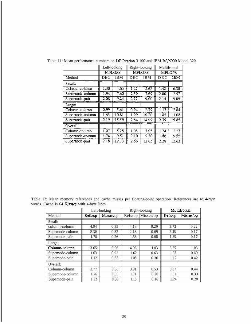
Table 11: Mean performance numbers on DECstation 3 100 and IBM RS/6000 Model 320.

Left-looking Right-looking MultifrontalMFLOPS MFLOPS MFLOPS

Method DEC 1 IBM DEC 1 IBM D E C 1 IBM

Table 12: Mean memory references and cache misses per floating-point operation. References are to 4-bytewords. Cache is 64 KBytes with 4-byte lines.

Left-looking Right-looking MuhifrontalMethod Refs/op Misses/op Refs/op Misses/op Refs/op Misses/opSmall:column-column 4.04 0.35 4.18 0.29 3.72 0.22Supemode-column 2.30 0.32 2.13 0.09 2.45 0.17Supemode-pair 1.78 0.26 1.58 0.08 1.85 0.17Large:column-colunln 3.65 0.96 4.06 1.03 3.25 1.03Supemode-column 1.63 0.92 1.62 0.63 1.67 0.69Supemode-pair 1.12 0.55 1.08 0.36 1.12 0.42Overall:Column-column 3.77 0.58 3.91 0.53 3.37 0.44Supemode-column 1.76 0.55 1.71 0.20 1.81 0.33Supemode-pair 1.22 0.39 1.15 0.16 1.24 0.28

2 0

above the ideal of 0.75, but they are still quite low.

The cache miss numbers for the supemode-pair methods are substantially lower as well. For example, thecache miss numbers are 30% lower for the left-looking method. This difference can be understood as follows.In the left-looking supemode-pair method, a pair of columns is now reused between supemode updates. Whena supemode is accessed, it frequently updates both columns, thus performing twice as many floating-pointoperations as would be done in the supemode-cohunn method. The cache miss numbers for the right-lookingand multifrontal methods have improved by roughly 15%, not nearly as much as they did for the left-lookingmethod. Recall that we described the cache behavior of these methods in terms of the sizes of the supemodesrelative to the size of the cache. Of the three cases we outlined, only the case where the supemode is largerthan the cache benefits from this modification. We note that the right-looking and multifrontal cache miss ratesare still significantly lower than the left-looking numbers.

The performance gains from the supemode-pair method on the DECstation 3100 are due mainly to thereduction in cache miss rates. We note that the right-looking method has the lowest miss rate of the threemethods, and achieves the highest performance as well. Recall that the decrease in memory references is notas relevant for the DECstation 3100, since the numbers we give assume a machine with 32 registers. The 16registers of the DECstation limit the memory reference benefits of updating a pair of columns at a time. Theperformance gains on the IBM RS/6000 are due to three factors. First, we have a significant decrease in thenumber of memory references. The second factor has to do with the fact that the supemode-pair kernel updatestwo destinations at once in the inner loop, allowing for a greater degree of instruction parallelism. The thirdfactor has to do with the decrease in the number of cache misses. The result is a 40% increase in performancefor the larger matrices. Unfortunately, we are unable to isolate the portions of the increase in performance thatcome from each of these three factors.

5.5 Supernode-supernode Methods

An obvious extension of the supemode-pair methods of the previous section would be to consider methods thatupdate some fixed number (greater than 2) of columns at a time. Rather than further investigating such ap-proaches, we instead consider primitives that modify an entire supemode by another supemode. Such primitiveswere originally proposed in [5]. By expressing the computation in terms of supemode-supemode operations,the C’ompz~t e I -1)dufe ( ) step becomes a matrix-matrix multiply. This kernel will allow us to not only reducetraffic between memory and the processor registers through unrolling, but it will also allow us to block thecomputation to reduce the traffic between memory and the cache. The use of supemode-supemode primitivesto reduce memory system traffic in a left-looking method has been proposed independently in [18]. We use asimple form of blocking in this section. We discuss alternative blocking strategies in a later section.

5.51 Implementation of Supemode-supemode Primitives

We begin our discussion of supernode-supemode methods by describing the implementation of the appropriateprimitives. To better motivate the blocking that will be done in a subsequent section, we describe the implemen-tation of supernode-supemode primitives in terms of dense matrix computations. We note that these primitiveswill all be implemented in terms of columns of the matrix in this section.

We begin with the Complete( ) primitive. Expressed in terms of the columns of the supemode, theC’ompld E ( ) performs the following operations:

1. for j= 1 to II do2 . for k= 1 to j- 1 do3 : cmod(j, k)4. cdiv(j)

An equivalent description of this computation, in terms of dense matrices, would be:

1 . -4 - hcto?*(A)

21

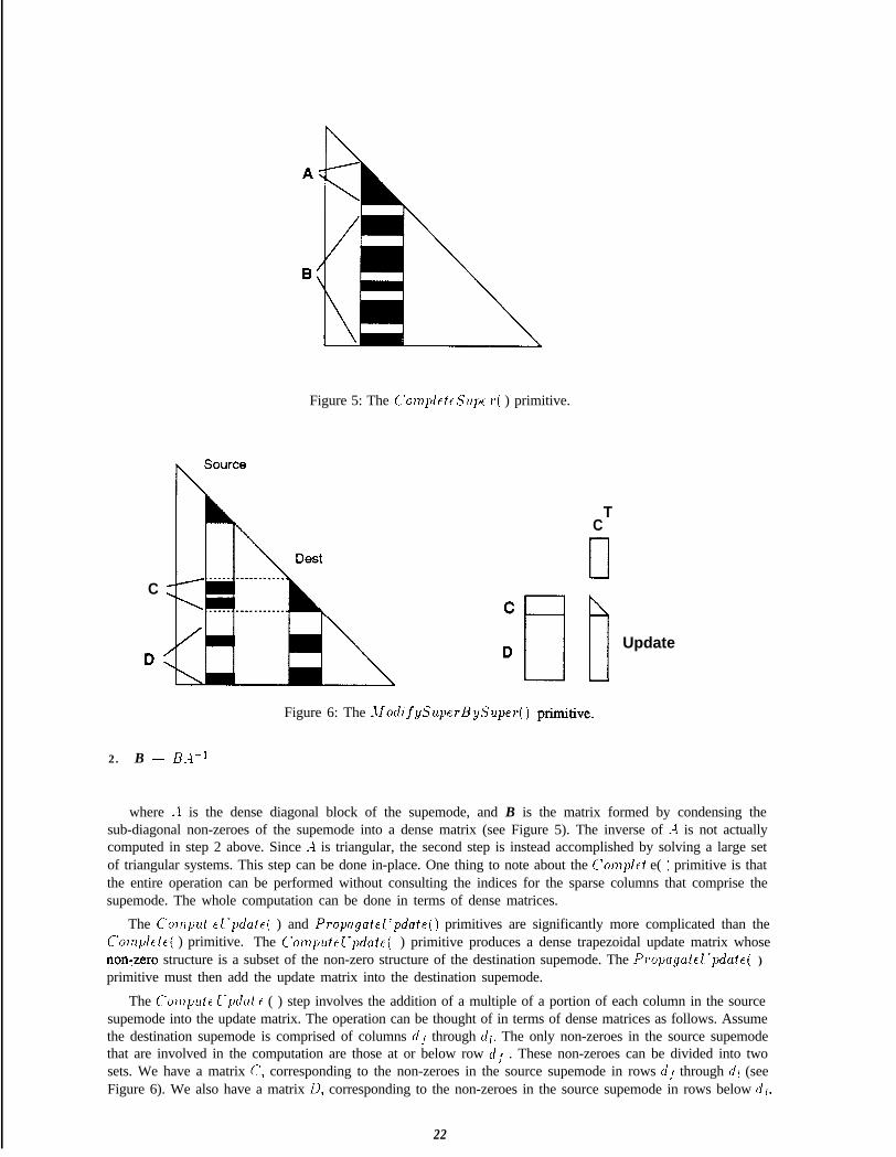
Figure 5: The C’O~IJ~C~CSUJX I’( ) primitive.

C

TC

0

7 Update

Figure 6: The -~~odifySuyerBySuper() primitive.

2. B - B-V-’

where -4 is the dense diagonal block of the supemode, and B is the matrix formed by condensing thesub-diagonal non-zeroes of the supemode into a dense matrix (see Figure 5). The inverse of -4 is not actuallycomputed in step 2 above. Since .4 is triangular, the second step is instead accomplished by solving a large setof triangular systems. This step can be done in-place. One thing to note about the Co?-rlylct e( ) primitive is thatthe entire operation can be performed without consulting the indices for the sparse columns that comprise thesupemode. The whole computation can be done in terms of dense matrices.

The C’o~ny~t ~l-l~dat~( ) and Proyagatel-pdate() primitives are significantly more complicated than theCo~nylete( ) primitive. The Comyrrtel~ydafr( ) primitive produces a dense trapezoidal update matrix whosenonYzero structure is a subset of the non-zero structure of the destination supemode. The Propayatelvpdafe( )primitive must then add the update matrix into the destination supemode.

The Co~~pnte I-yda2 E ( ) step involves the addition of a multiple of a portion of each column in the sourcesupemode into the update matrix. The operation can be thought of in terms of dense matrices as follows. Assumethe destination supemode is comprised of columns d, through dl. The only non-zeroes in the source supemodethat are involved in the computation are those at or below row df . These non-zeroes can be divided into twosets. We have a matrix C’, corresponding to the non-zeroes in the source supemode in rows dj through cl/ (seeFigure 6). We also have a matrix D, corresponding to the non-zeroes in the source supemode in rows below dl.

22

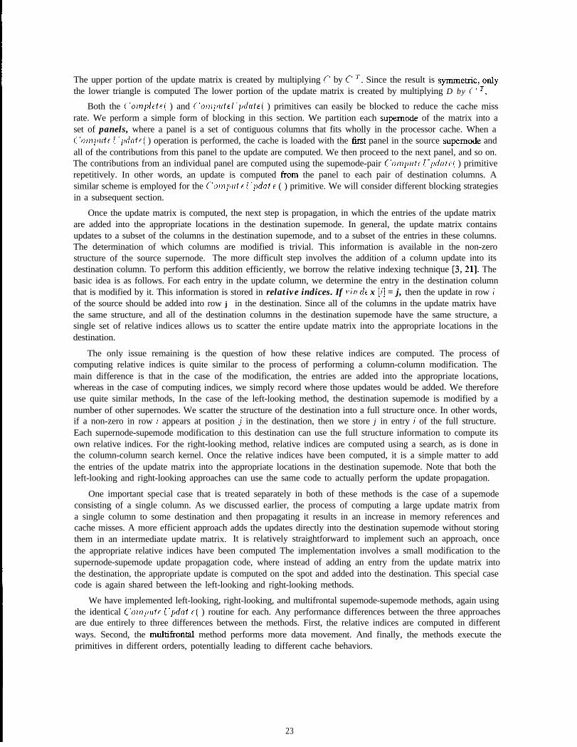
The upper portion of the update matrix is created by multiplying C‘ by C’ T. Since the result is symmetric, onlythe lower triangle is computed The lower portion of the update matrix is created by multiplying D by l’ ’ T.

Both the C’O???J)/~~F( ) and C’ol,,l)trt~~-l~c/cli~( ) primitives can easily be blocked to reduce the cache missrate. We perform a simple form of blocking in this section. We partition each supernode of the matrix into aset of panels, where a panel is a set of contiguous columns that fits wholly in the processor cache. When aC’o~~l)~f~ I -~K/c/~F( ) operation is performed, the cache is loaded with the tit panel in the source supernode andall of the contributions from this panel to the update are computed. We then proceed to the next panel, and so on.The contributions from an individual panel are computed using the supemode-pair C’o~,l~rt~ l-~~lut~( ) primitiverepetitively. In other words, an update is computed from the panel to each pair of destination columns. Asimilar scheme is employed for the (“ou?I)u~ c I7yduf E ( ) primitive. We will consider different blocking strategiesin a subsequent section.

Once the update matrix is computed, the next step is propagation, in which the entries of the update matrixare added into the appropriate locations in the destination supemode. In general, the update matrix containsupdates to a subset of the columns in the destination supemode, and to a subset of the entries in these columns.The determination of which columns are modified is trivial. This information is available in the non-zerostructure of the source supernode. The more difficult step involves the addition of a column update into itsdestination column. To perform this addition efficiently, we borrow the relative indexing technique [3,21]. Thebasic idea is as follows. For each entry in the update column, we determine the entry in the destination columnthat is modified by it. This information is stored in relative indices. If rin de x [i] = j, then the update in row iof the source should be added into row j in the destination. Since all of the columns in the update matrix havethe same structure, and all of the destination columns in the destination supemode have the same structure, asingle set of relative indices allows us to scatter the entire update matrix into the appropriate locations in thedestination.

The only issue remaining is the question of how these relative indices are computed. The process ofcomputing relative indices is quite similar to the process of performing a column-column modification. Themain difference is that in the case of the modification, the entries are added into the appropriate locations,whereas in the case of computing indices, we simply record where those updates would be added. We thereforeuse quite similar methods, In the case of the left-looking method, the destination supemode is modified by anumber of other supernodes. We scatter the structure of the destination into a full structure once. In other words,if a non-zero in row i appears at position j in the destination, then we store j in entry i of the full structure.Each supernode-supemode modification to this destination can use the full structure information to compute itsown relative indices. For the right-looking method, relative indices are computed using a search, as is done inthe column-column search kernel. Once the relative indices have been computed, it is a simple matter to addthe entries of the update matrix into the appropriate locations in the destination supemode. Note that both theleft-looking and right-looking approaches can use the same code to actually perform the update propagation.

One important special case that is treated separately in both of these methods is the case of a supemodeconsisting of a single column. As we discussed earlier, the process of computing a large update matrix froma single column to some destination and then propagating it results in an increase in memory references andcache misses. A more efficient approach adds the updates directly into the destination supemode without storingthem in an intermediate update matrix. It is relatively straightforward to implement such an approach, oncethe appropriate relative indices have been computed The implementation involves a small modification to thesupernode-supemode update propagation code, where instead of adding an entry from the update matrix intothe destination, the appropriate update is computed on the spot and added into the destination. This special casecode is again shared between the left-looking and right-looking methods.

We have implemented left-looking, right-looking, and multifrontal supemode-supemode methods, again usingthe identical C’OMI)&F ZTpduf E( ) routine for each. Any performance differences between the three approachesare due entirely to three differences between the methods. First, the relative indices are computed in differentways. Second, the multifrontal method performs more data movement. And finally, the methods execute theprimitives in different orders, potentially leading to different cache behaviors.

23

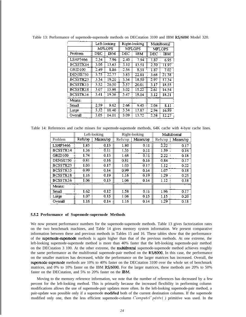
Table 13: Performance of supemode-supemode methods on DECstation 3100 and IBM RS/6000 Model 320.

Table 14: References and cache misses for supemode-supemode methods, 64K cache with 4-byte cache lines.

Left-looking Right-looking MultifrontalProblem Refslop 1 Misses/op Refs/op 1 Misses/op Refs/op 1 Misses/op

55.2 Performance of Supemode-supernode Methods

We now present performance numbers for the supemode-supemode methods. Table 13 gives factorization rateson the two benchmark machines, and Table 14 gives memory system information. We present comparativeinformation between these and previous methods in Tables 15 and 16. These tables show that the performanceof the supernode-supernode methods is again higher than that of the previous methods. At one extreme, theleft-looking supemode-supemode method is more than 40% faster that the left-looking supemode-pair methodon the DECstation 3 100. At the other extreme, the multifrontal supemode-supemode method achieves roughlythe same performance as the multifrontal supemode-pair method on the RS/6000. In this case, the performanceon the smaller matrices has decreased, while the performance on the larger matrices has increased. Overall, thesupernode-supemode methods are 10% to 40% faster on the DECstation 3100 over the whole set of benchmarkmatrices, and 0% to 10% faster on the IBM RS/6000. For the larger matrices, these methods are 20% to 50%faster on the DECstation, and 5% to 20% faster on the IBM.

Moving to the memory reference information, we note that the number of references has decreased by a fewpercent for the left-looking method. This is primarily because the increased flexibility in performing columnmodifications allows the use of supemode-pair updates more often. In the left-looking supemode-pair method, apair-update was possible only if a supemode modified both of the current destination columns. If the supemodemodified only one, then the less efficient supemode-column Con?yufelvydate( ) primitive was used. In the

24

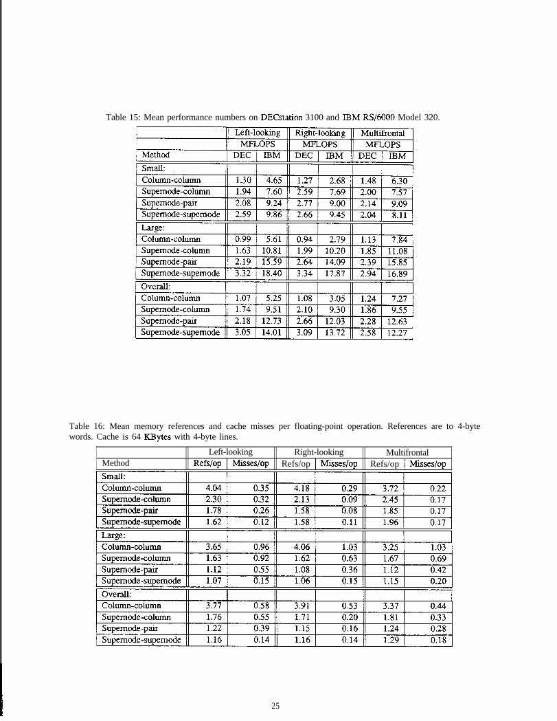
Table 15: Mean performance numbers on DECstation 3100 and IBM RS/6000 Model 320.

Table 16: Mean memory references and cache misses per floating-point operation. References are to 4-bytewords. Cache is 64 KBytes with 4-byte lines.

Left-looking Right-looking MultifrontalMethod Refs/op 1 Misses/op Refs/op 1 Misses/op Refs/op 1 Misses/op

25

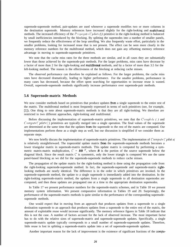
supemode-supemode method, pair-updates are used whenever a supemode modifies two or more columns inthe destination supemode. Memory references have increased slightly for the right-looking and multifrontalmethods. The increased efficiency of the Propc~~nt F Ivpdui~ ( ) primitive in the right-looking method is balancedby small inefficiencies introduced by the blocking. By splitting the supemodes into a number of smaller panels,we frequently reduce the effectiveness of the loop unrolling. We also frequently waste effort, particularly in thesmaller problems, looking for increased reuse that is not present. The effect can be seen more clearly in thememory reference numbers for the multifrontal method, which does not gain any offsetting memory referenceadvantage in moving to supemode-supemode primitives.

We note that the cache miss rates for the three methods are similar, and in all cases they are substantiallylower than those achieved by the supemode-pair methods. For the larger problems, miss rates have decrease bya factor of more than 2 for the right-looking and multifrontal methods, and by a factor of more than 3.5 for theleft-looking method. The reason is the effectiveness of the blocking at reducing cache misses.

The observed performance can therefore be explained as follows. For the larger problems, the cache missrates have decreased dramatically, leading to higher performance. For the smaller problems, performance inmany cases has decreased, because the effort spent searching for opportunities to increase reuse is wasted.Overall, supernode-supemode methods significantly increase performance over supemode-pair methods.

5.6 Supernode-matrix Methods

We now consider methods based on primitives that produce updates from a single supemode to the entire rest ofthe matrix. The multifrontal method is most frequently expressed in terms of such primitives (see, for example,El]). One thing to note about supemode-matrix methods is that they are all right-looking. We therefore arerestricted to two different approaches, right-looking and multifrontal.

Before discussing the implementation of supemode-matrix primitives, we note that the Complete ( ) andC’o~-ryuf~~~y~/ut~( ) primitives are typically merged into a single operation. The final values of the supemodeare determined at the same time that the updates from the supemode to the rest of the matrix are computed. Ourimplementations perform these as a single step as well, but our discussion is simplified if we consider them asseparate steps.

We now briefly discuss the implementation of supemode-matrix primitives. The implementation of Cojnputr l’pduf e(is relatively straightforward. The trapezoidal update matrix from the supemode-supemode methods becomes alower triangular matrix in supemode-matrix methods. This update matrix is computed by performing a sym-metric matrix-matrix multiplication, C = BB T, where B is the portion of the source supemode below thediagonal block. Since the result matrix c’ is symmetric, only the lower triangle is computed We use the samepanel-based blocking as we did for the supemode-supemode methods to reduce cache misses.

The propagation of the update matrix for the right-looking method is done using the propagation code fromthe right-looking supernode-supemode method. In fact, the supemode-supemode and supemode-matrix right-looking methods are nearly identical. The difference is in the order in which primitives are invoked. In thesupemode-supemode method, the update to a single supemode is immediately added into the destination. In theright-looking supernode-matrix method, the updates from a single supemode to all destination supemodes arecomputed, and then these updates are propagated one at a time to the appropriate destination supemodes.

In Table 17 we present performance numbers for the supemode-matrix schemes, and in Table 18 we presentmemory system information. We present comparative information in Tables 19 and 20. Surprisingly, theperformance of the supemode-matrix methods is quite similar to the performance of the corresponding supemode-supemode methods.

One would expect that in moving from an approach that produces updates from a supernode to a singledestination supemode to an approach that produces updates from a supemode to the entire rest of the matrix, theamount of exploitable reuse would increase significantly. The memory reference figures in Table 18 indicate thatthis is not the case. A number of factors account for the lack of observed increase. The most important factorhas to do with the relative sizes of supernode-matrix and supemode-supemode updates. Specifically, a singlesupemode-matrix update typically corresponds to a small number of supemode-supemode updates. Therefore,little reuse is lost in splitting a supemode-matrix update into a set of supemode-supemode updates.

Another important reason for the lack of improvement is the existence of significant fractions of the compu-

26

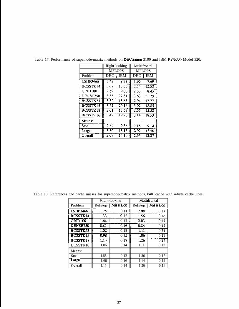
Table 17: Performance of supemode-matrix methods on DECstation 3100 and IBM RS/6000 Model 320.

Right-looking MultifrontalMFLOPS MFLOPS

Problem DEC 1 IBM DEC ( IBM

Table 18: References and cache misses for supemode-matrix methods, 64K cache with 4-byte cache lines.

ProblemRight-looking Multi!kontal

Refs/op 1 Misses/op Refs/op I Misses/op

BCSSTK16Means:SmallLawOverall

1.06 0.14 1.11 0.17

1.55 0.12 1.86 0.171.06 0.16 1.14 0.191.15 0.14 1.26 0.18

27

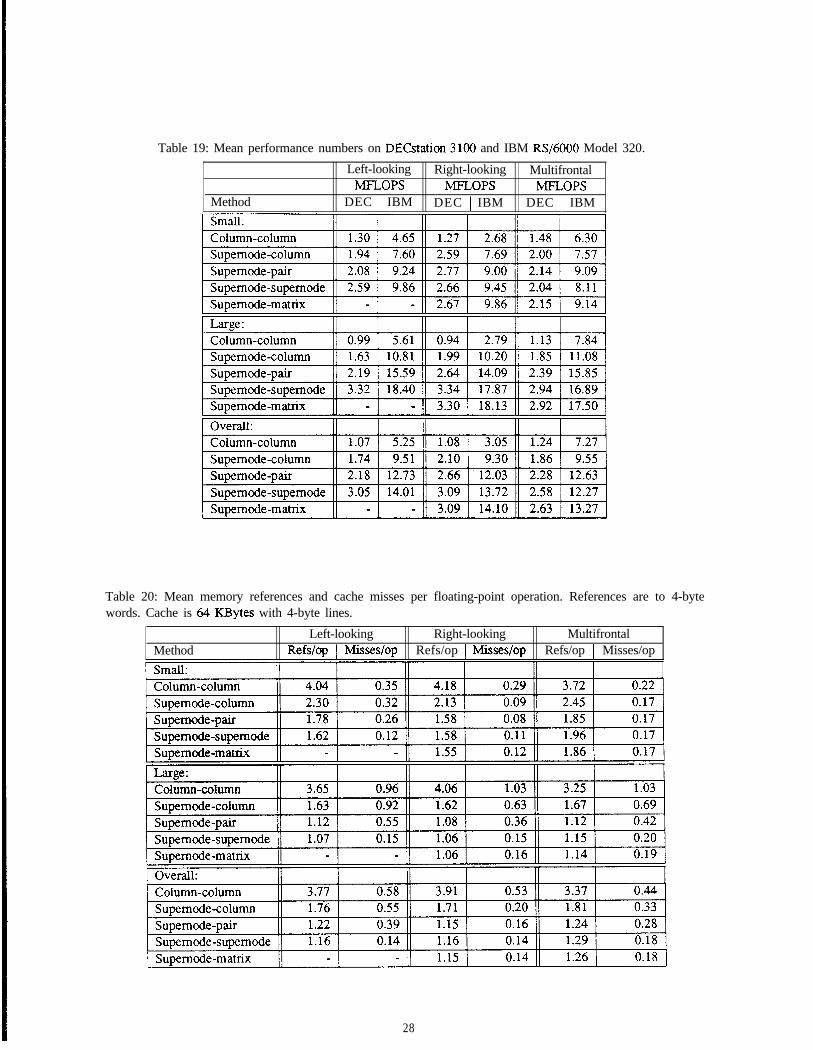
Table 19: Mean performance numbers on DECstation 3100 and IBM RS/6000 Model 320.

Left-looking Right-looking MultifrontalMFLOPS MFLOPS MFLOPS

Method DEC 1 IBM DEC 1 IBM DEC 1 IBM

Table 20: Mean memory references and cache misses per floating-point operation. References are to 4-bytewords. Cache is @ ISBytes with 4-byte lines.

Left-looking Right-looking MultifrontalMethod Refs/op 1 Misses/op Refs/op ] Misses/op Refs/op I Misses/op

28

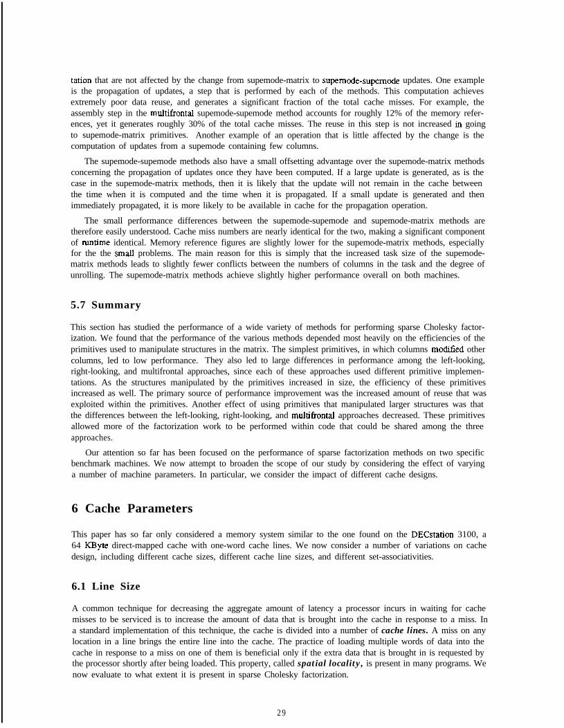
tation that are not affected by the change from supemode-matrix to supemode-supernode updates. One exampleis the propagation of updates, a step that is performed by each of the methods. This computation achievesextremely poor data reuse, and generates a significant fraction of the total cache misses. For example, theassembly step in the multifrontal supemode-supemode method accounts for roughly 12% of the memory refer-ences, yet it generates roughly 30% of the total cache misses. The reuse in this step is not increased in goingto supemode-matrix primitives. Another example of an operation that is little affected by the change is thecomputation of updates from a supemode containing few columns.

The supemode-supemode methods also have a small offsetting advantage over the supemode-matrix methodsconcerning the propagation of updates once they have been computed. If a large update is generated, as is thecase in the supemode-matrix methods, then it is likely that the update will not remain in the cache betweenthe time when it is computed and the time when it is propagated. If a small update is generated and thenimmediately propagated, it is more likely to be available in cache for the propagation operation.

The small performance differences between the supemode-supemode and supemode-matrix methods aretherefore easily understood. Cache miss numbers are nearly identical for the two, making a significant componentof runtime identical. Memory reference figures are slightly lower for the supemode-matrix methods, especiallyfor the the smalI problems. The main reason for this is simply that the increased task size of the supemode-matrix methods leads to slightly fewer conflicts between the numbers of columns in the task and the degree ofunrolling. The supemode-matrix methods achieve slightly higher performance overall on both machines.

5.7 Summary

This section has studied the performance of a wide variety of methods for performing sparse Cholesky factor-ization. We found that the performance of the various methods depended most heavily on the efficiencies of theprimitives used to manipulate structures in the matrix. The simplest primitives, in which columns modSed othercolumns, led to low performance. They also led to large differences in performance among the left-looking,right-looking, and multifrontal approaches, since each of these approaches used different primitive implemen-tations. As the structures manipulated by the primitives increased in size, the efficiency of these primitivesincreased as well. The primary source of performance improvement was the increased amount of reuse that wasexploited within the primitives. Another effect of using primitives that manipulated larger structures was thatthe differences between the left-looking, right-looking, and multifrontal approaches decreased. These primitivesallowed more of the factorization work to be performed within code that could be shared among the threeapproaches.

Our attention so far has been focused on the performance of sparse factorization methods on two specificbenchmark machines. We now attempt to broaden the scope of our study by considering the effect of varyinga number of machine parameters. In particular, we consider the impact of different cache designs.

6 Cache Parameters

This paper has so far only considered a memory system similar to the one found on the DECstation 3100, a64 KByte direct-mapped cache with one-word cache lines. We now consider a number of variations on cachedesign, including different cache sizes, different cache line sizes, and different set-associativities.

6.1 Line Size

A common technique for decreasing the aggregate amount of latency a processor incurs in waiting for cachemisses to be serviced is to increase the amount of data that is brought into the cache in response to a miss. Ina standard implementation of this technique, the cache is divided into a number of cache lines. A miss on anylocation in a line brings the entire line into the cache. The practice of loading multiple words of data into thecache in response to a miss on one of them is beneficial only if the extra data that is brought in is requested bythe processor shortly after being loaded. This property, called spatial locality, is present in many programs. Wenow evaluate to what extent it is present in sparse Cholesky factorization.

2 9

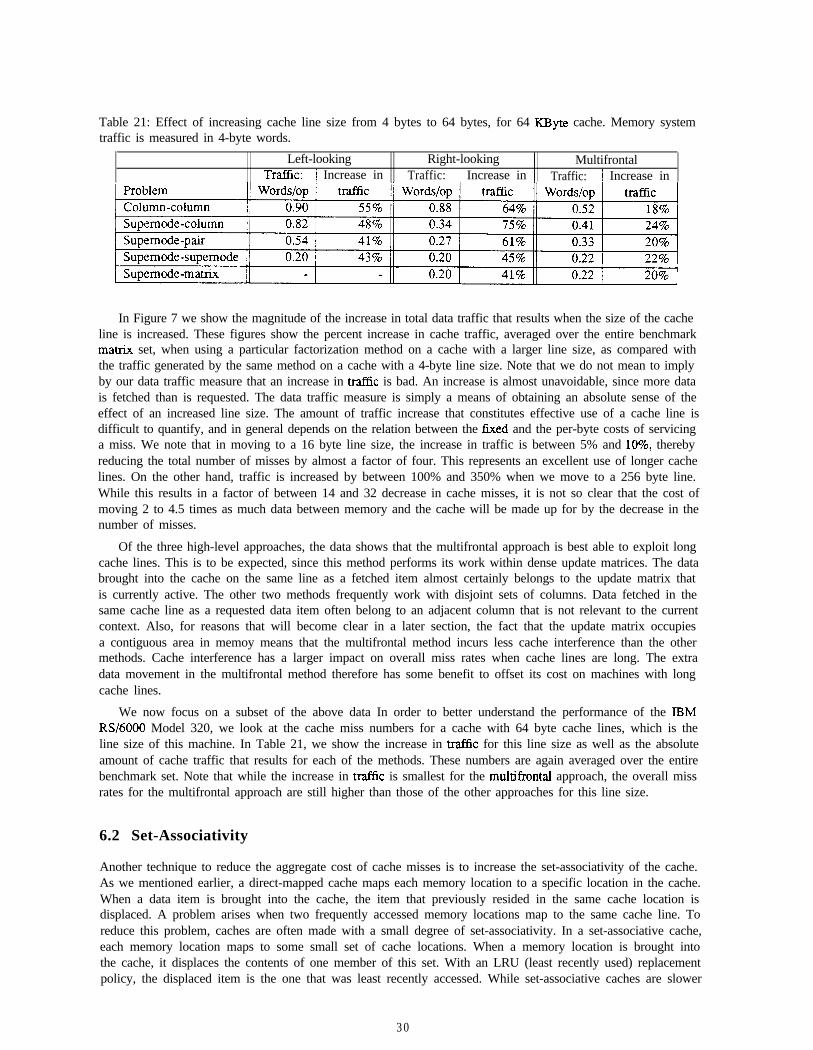
Table 21: Effect of increasing cache line size from 4 bytes to 64 bytes, for 64 KByte cache. Memory systemtraffic is measured in 4-byte words.

Left-looking Right-looking MultifrontalTraffic: 1 Increase in Traffic: 1 Increase in Traffic: 1 Increase in

In Figure 7 we show the magnitude of the increase in total data traffic that results when the size of the cacheline is increased. These figures show the percent increase in cache traffic, averaged over the entire benchmarkmatrix set, when using a particular factorization method on a cache with a larger line size, as compared withthe traffic generated by the same method on a cache with a 4-byte line size. Note that we do not mean to implyby our data traffic measure that an increase in traffic is bad. An increase is almost unavoidable, since more datais fetched than is requested. The data traffic measure is simply a means of obtaining an absolute sense of theeffect of an increased line size. The amount of traffic increase that constitutes effective use of a cache line isdifficult to quantify, and in general depends on the relation between the lixed and the per-byte costs of servicinga miss. We note that in moving to a 16 byte line size, the increase in traffic is between 5% and lo%, therebyreducing the total number of misses by almost a factor of four. This represents an excellent use of longer cachelines. On the other hand, traffic is increased by between 100% and 350% when we move to a 256 byte line.While this results in a factor of between 14 and 32 decrease in cache misses, it is not so clear that the cost ofmoving 2 to 4.5 times as much data between memory and the cache will be made up for by the decrease in thenumber of misses.

Of the three high-level approaches, the data shows that the multifrontal approach is best able to exploit longcache lines. This is to be expected, since this method performs its work within dense update matrices. The databrought into the cache on the same line as a fetched item almost certainly belongs to the update matrix thatis currently active. The other two methods frequently work with disjoint sets of columns. Data fetched in thesame cache line as a requested data item often belong to an adjacent column that is not relevant to the currentcontext. Also, for reasons that will become clear in a later section, the fact that the update matrix occupiesa contiguous area in memoy means that the multifrontal method incurs less cache interference than the othermethods. Cache interference has a larger impact on overall miss rates when cache lines are long. The extradata movement in the multifrontal method therefore has some benefit to offset its cost on machines with longcache lines.

We now focus on a subset of the above data In order to better understand the performance of the IBMRS/6000 Model 320, we look at the cache miss numbers for a cache with 64 byte cache lines, which is theline size of this machine. In Table 21, we show the increase in traffic for this line size as well as the absoluteamount of cache traffic that results for each of the methods. These numbers are again averaged over the entirebenchmark set. Note that while the increase in traffic is smallest for the multifrontal approach, the overall missrates for the multifrontal approach are still higher than those of the other approaches for this line size.

6.2 Set-Associativity

Another technique to reduce the aggregate cost of cache misses is to increase the set-associativity of the cache.As we mentioned earlier, a direct-mapped cache maps each memory location to a specific location in the cache.When a data item is brought into the cache, the item that previously resided in the same cache location isdisplaced. A problem arises when two frequently accessed memory locations map to the same cache line. Toreduce this problem, caches are often made with a small degree of set-associativity. In a set-associative cache,each memory location maps to some small set of cache locations. When a memory location is brought intothe cache, it displaces the contents of one member of this set. With an LRU (least recently used) replacementpolicy, the displaced item is the one that was least recently accessed. While set-associative caches are slower

3 0

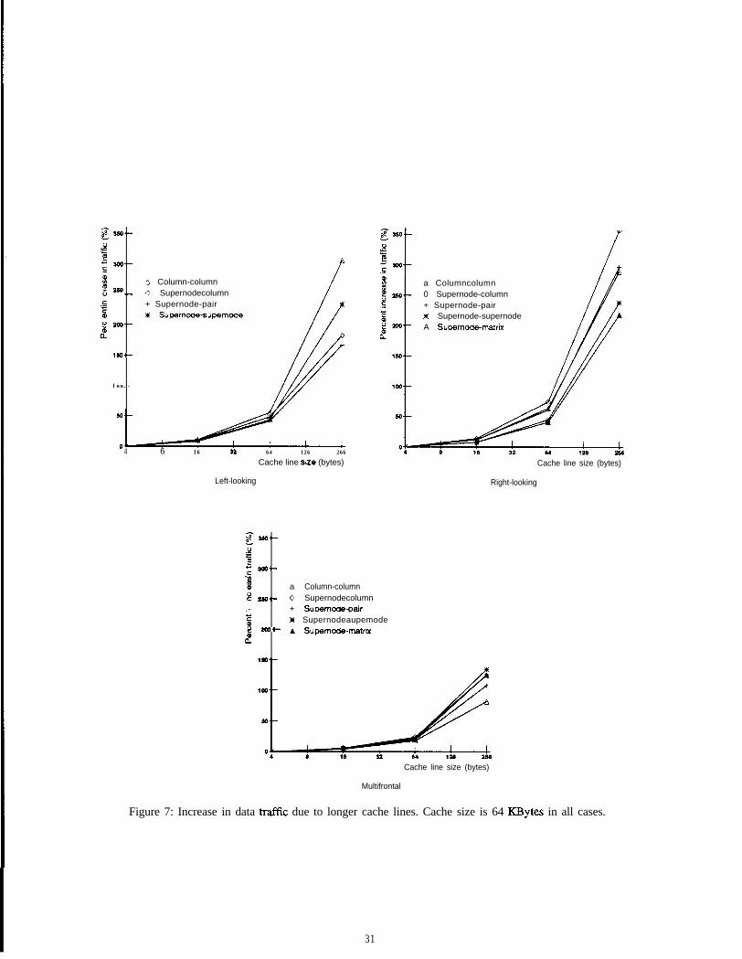
s 260.-e.Y=i!- wo.-.s32 ._

A Column-columnz= 0 Supernodecolumn

.c + Supernode-pair5 m Supernode-supernode2 200.-a”

160.-

loo.-

4 6 16 12 64 126 266

Cache line s!ze (bytes)

Left-looking

a Columncolumn0 Supernode-column+ Supernode-pairm Supernode-supernodeA Supernode-matnx

Cache line size (bytes)

Right-looking

s so--ez!I- 600.-.s0,0 a Column-columnL2 2m.- 0 Supernodecolumn.- + Supernodepair

E m Supernodeaupemode@ 200-W A Supernode-matron2

Cache line size (bytes)

Multifrontal

Figure 7: Increase in data traflic due to longer cache lines. Cache size is 64 KBytes in all cases.

31

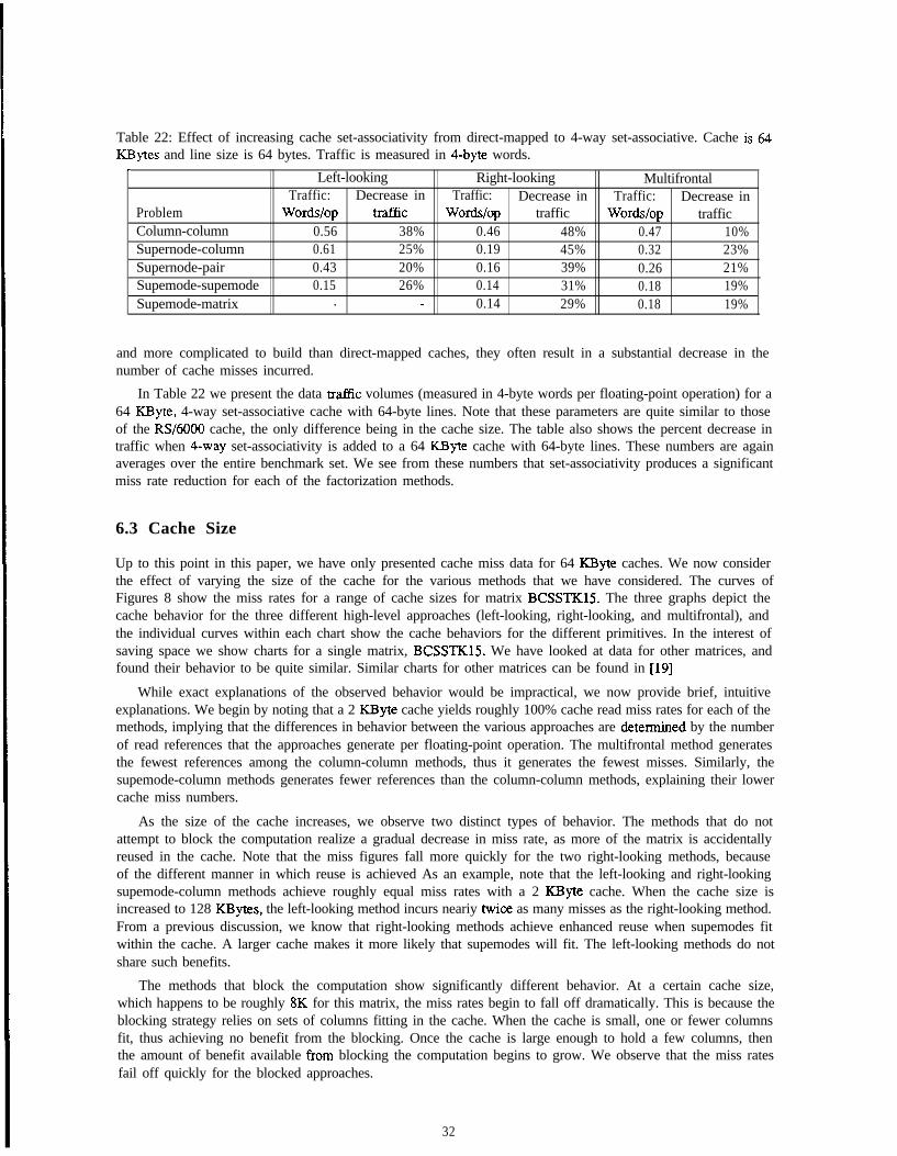
Table 22: Effect of increasing cache set-associativity from direct-mapped to 4-way set-associative. Cache is 154KBytes and line size is 64 bytes. Traffic is measured in 4-byte words.

rLeft-looking Right-looking Multifrontal

Traffic: Decrease in Traffic: Decrease in Traffic: Decrease inProblem Words/op mffic Words/op traffic Words/op trafficColumn-column 0.56 38% 0.46 48% 0.47 10%Supernode-column 0.61 25% 0.19 45% 0.32 23%Supernode-pair 0.43 20% 0.16 39% 0.26 21%Supemode-supemode 0.15 26% 0.14 31% 0.18 19%Supemode-matrix . - 0.14 29% 0.18 19%

and more complicated to build than direct-mapped caches, they often result in a substantial decrease in thenumber of cache misses incurred.

In Table 22 we present the data traftic volumes (measured in 4-byte words per floating-point operation) for a64 KByte, 4-way set-associative cache with 64-byte lines. Note that these parameters are quite similar to thoseof the RS/6000 cache, the only difference being in the cache size. The table also shows the percent decrease intraffic when 4-way set-associativity is added to a 64 KByte cache with 64-byte lines. These numbers are againaverages over the entire benchmark set. We see from these numbers that set-associativity produces a significantmiss rate reduction for each of the factorization methods.

6.3 Cache Size

Up to this point in this paper, we have only presented cache miss data for 64 KByte caches. We now considerthe effect of varying the size of the cache for the various methods that we have considered. The curves ofFigures 8 show the miss rates for a range of cache sizes for matrix BCSSTKlS. The three graphs depict thecache behavior for the three different high-level approaches (left-looking, right-looking, and multifrontal), andthe individual curves within each chart show the cache behaviors for the different primitives. In the interest ofsaving space we show charts for a single matrix, BCSSTKlS. We have looked at data for other matrices, andfound their behavior to be quite similar. Similar charts for other matrices can be found in [19]

While exact explanations of the observed behavior would be impractical, we now provide brief, intuitiveexplanations. We begin by noting that a 2 KByte cache yields roughly 100% cache read miss rates for each of themethods, implying that the differences in behavior between the various approaches are determined by the numberof read references that the approaches generate per floating-point operation. The multifrontal method generatesthe fewest references among the column-column methods, thus it generates the fewest misses. Similarly, thesupemode-column methods generates fewer references than the column-column methods, explaining their lowercache miss numbers.

As the size of the cache increases, we observe two distinct types of behavior. The methods that do notattempt to block the computation realize a gradual decrease in miss rate, as more of the matrix is accidentallyreused in the cache. Note that the miss figures fall more quickly for the two right-looking methods, becauseof the different manner in which reuse is achieved As an example, note that the left-looking and right-lookingsupemode-column methods achieve roughly equal miss rates with a 2 KByte cache. When the cache size isincreased to 128 KBytes, the left-looking method incurs neariy twice as many misses as the right-looking method.From a previous discussion, we know that right-looking methods achieve enhanced reuse when supemodes fitwithin the cache. A larger cache makes it more likely that supemodes will fit. The left-looking methods do notshare such benefits.

The methods that block the computation show significantly different behavior. At a certain cache size,which happens to be roughly 8K for this matrix, the miss rates begin to fall off dramatically. This is because theblocking strategy relies on sets of columns fitting in the cache. When the cache is small, one or fewer columnsfit, thus achieving no benefit from the blocking. Once the cache is large enough to hold a few columns, thenthe amount of benefit available from blocking the computation begins to grow. We observe that the miss ratesfail off quickly for the blocked approaches.

32

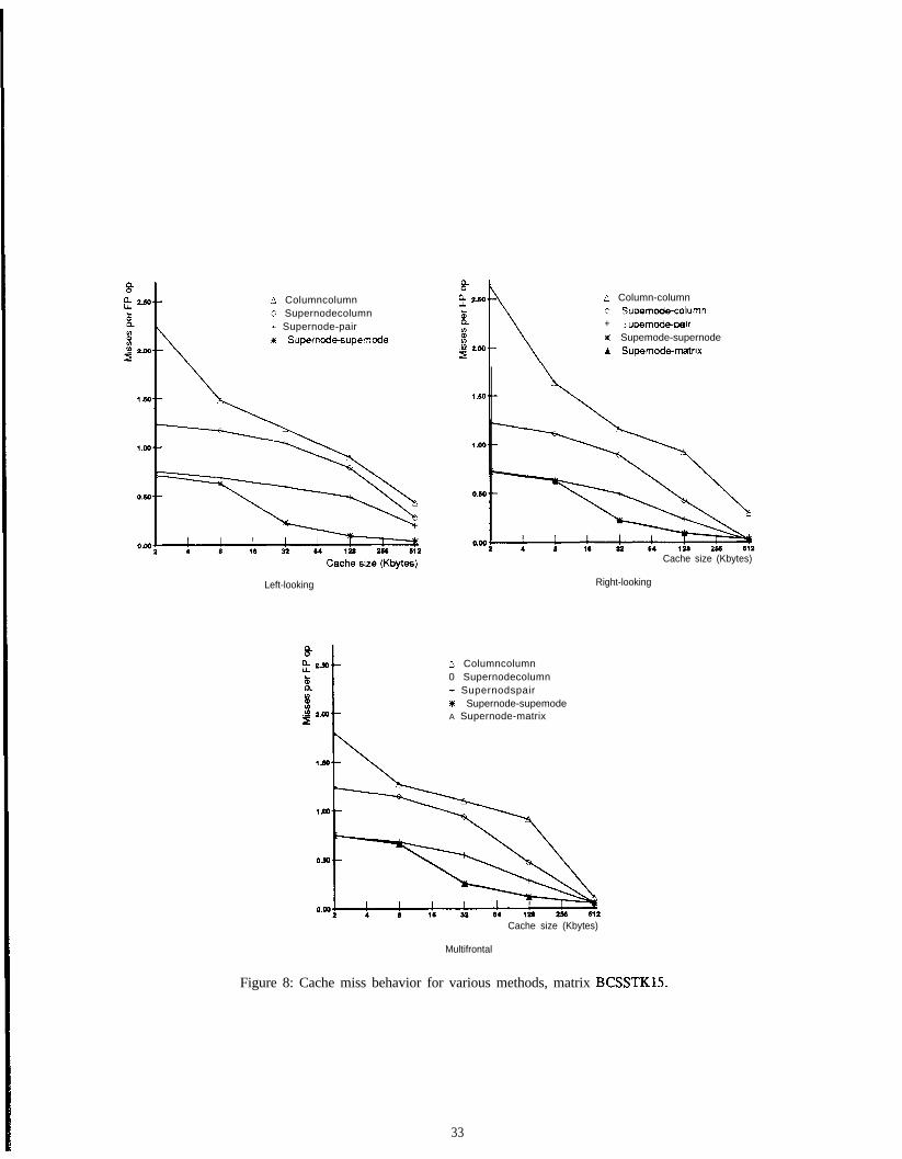
fi Columncolumn0 Supernodecolumn+ Supernode-pair% Supernode-supernode

2 Column-columnc Supemde-adumn+ 3upemode-pairm Supemode-supernodeA Supemode-matnx

Left-looking Right-looking

Cache size (Kbytes)

3 Columncolumn0 Supernodecolumn+ Supernodspairm Supernode-supemodeA Supernode-matrix

Cache size (Kbytes)

Multifrontal

Figure 8: Cache miss behavior for various methods, matrix BCSSTKlS.

33

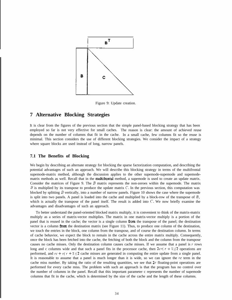
Figure 9: Update creation.

7 Alternative Blocking Strategies

It is clear from the figures of the previous section that the simple panel-based blocking strategy that has beenemployed so far is not very effective for small caches. The reason is clear: the amount of achieved reusedepends on the number of columns that fit in the cache. In a small cache, few columns fit so the reuse isminimal. This section considers the use of different blocking strategies. We consider the impact of a strategywhere square blocks are used instead of long, narrow panels.

7.1 The Benefits of Blocking

We begin by describing an alternate strategy for blocking the sparse factorization computation, and describing thepotential advantages of such an approach. We will describe this blocking strategy in terms of the multifrontalsupemode-matrix method, although the discussion applies to the other supemode-supemode and supemode-matrix methods as well. Recall that in the multifrontal method, a supemode is used to create an update matrix.Consider the matrices of Figure 9. The B matrix represents the non-zeroes within the supemode. The matrixB is multiplied by its transpose to produce the update matrix c. In the previous section, this computation wasblocked by splitting B vertically, into a number of narrow panels. Figure 10 shows the case where the supemodeis split into two panels. A panel is loaded into the cache and multiplied by a block-row of the transpose of B,which is actually the transpose of the panel itself. The result is added into c’. We now briefly examine theadvantages and disadvantages of such an approach.

To better understand the panel-oriented blocked matrix multiply, it is convenient to think of the matrix-matrixmultiply as a series of matrix-vector multiplies. The matrix in one matrix-vector multiply is a portion of thepanel that is reused in the cache; the vector is a single column from the transpose of the panel; the destinationvector is a column Tom the destination matrix (see Figure 11). Thus, to produce one column of the destination,we touch the entries in the block, one column from the transpose, and of course the destination column. In termsof cache behavior, we expect the block to remain in the cache across the entire matrix multiply. Consequently,once the block has been fetched into the cache, the fetching of both the block and the column from the transposecauses no cache misses. Only the destination column causes cache misses. If we assume that a panel is I* rowslong and c columns wide and that such a panel fits in the processor cache, then 2cl,( 1’ + 1)/2 operations areperformed, and rc -t r( r + 1)/2 cache misses are generated in computing the entire update from a single panel.It is reasonable to assume that a panel is much longer than it is wide, so we can ignore the 1‘~’ term in thecache miss number. By taking the ratio of the resulting quantities, we see that 2c floating-point operations areperformed for every cache miss. The problem with such an approach is that the program has no control overthe number of columns in the panel. Recall that this important parameter c represents the number of supemodecolumns that fit in the cache, which is determined by the size of the cache and the length of these columns.

3 4

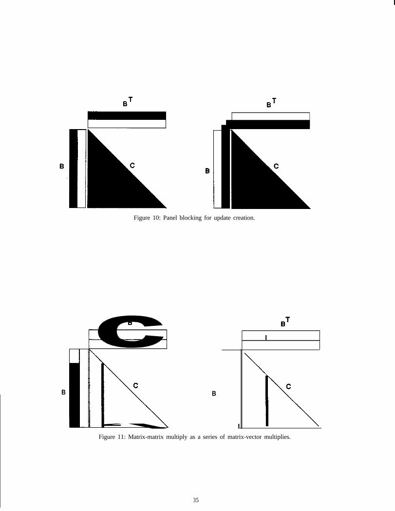
BT

B

I

Figure 10: Panel blocking for update creation.

I

C

I

B

BT

I

Figure 11: Matrix-matrix multiply as a series of matrix-vector multiplies.

35

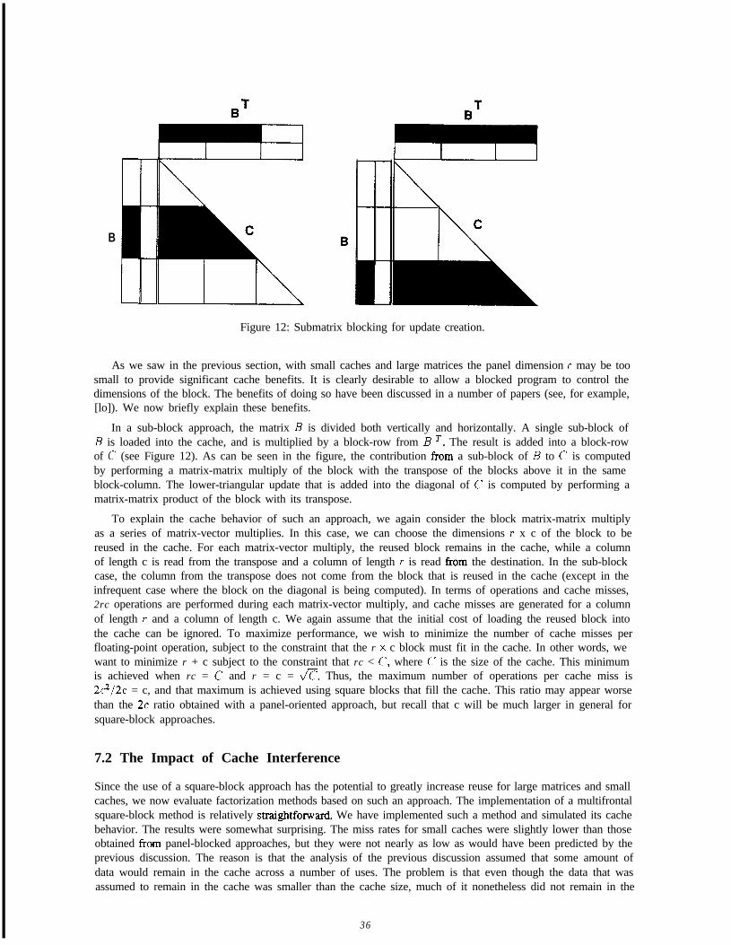
B

!

Figure 12: Submatrix blocking for update creation.

As we saw in the previous section, with small caches and large matrices the panel dimension c may be toosmall to provide significant cache benefits. It is clearly desirable to allow a blocked program to control thedimensions of the block. The benefits of doing so have been discussed in a number of papers (see, for example,[lo]). We now briefly explain these benefits.

In a sub-block approach, the matrix B is divided both vertically and horizontally. A single sub-block ofB is loaded into the cache, and is multiplied by a block-row from B T. The result is added into a block-rowof C (see Figure 12). As can be seen in the figure, the contribution from a sub-block of B to c’ is computedby performing a matrix-matrix multiply of the block with the transpose of the blocks above it in the sameblock-column. The lower-triangular update that is added into the diagonal of C’ is computed by performing amatrix-matrix product of the block with its transpose.

To explain the cache behavior of such an approach, we again consider the block matrix-matrix multiplyas a series of matrix-vector multiplies. In this case, we can choose the dimensions r x c of the block to bereused in the cache. For each matrix-vector multiply, the reused block remains in the cache, while a columnof length c is read from the transpose and a column of length T is read from the destination. In the sub-blockcase, the column from the transpose does not come from the block that is reused in the cache (except in theinfrequent case where the block on the diagonal is being computed). In terms of operations and cache misses,2rc operations are performed during each matrix-vector multiply, and cache misses are generated for a columnof length r and a column of length c. We again assume that the initial cost of loading the reused block intothe cache can be ignored. To maximize performance, we wish to minimize the number of cache misses perfloating-point operation, subject to the constraint that the r x c block must fit in the cache. In other words, wewant to minimize r + c subject to the constraint that rc < c’, where C’ is the size of the cache. This minimumis achieved when rc = c and r = c = fi. Thus, the maximum number of operations per cache miss is2?/2c = c, and that maximum is achieved using square blocks that fill the cache. This ratio may appear worsethan the 2c ratio obtained with a panel-oriented approach, but recall that c will be much larger in general forsquare-block approaches.

7.2 The Impact of Cache Interference

Since the use of a square-block approach has the potential to greatly increase reuse for large matrices and smallcaches, we now evaluate factorization methods based on such an approach. The implementation of a multifrontalsquare-block method is relatively straightfonvard. We have implemented such a method and simulated its cachebehavior. The results were somewhat surprising. The miss rates for small caches were slightly lower than thoseobtained from panel-blocked approaches, but they were not nearly as low as would have been predicted by theprevious discussion. The reason is that the analysis of the previous discussion assumed that some amount ofdata would remain in the cache across a number of uses. The problem is that even though the data that wasassumed to remain in the cache was smaller than the cache size, much of it nonetheless did not remain in the

36

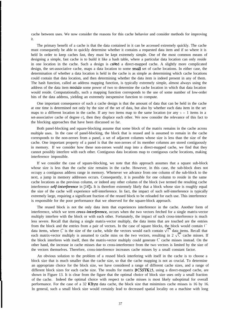
cache between uses. We now consider the reasons for this cache behavior and consider methods for improvingit.

The primary benefit of a cache is that the data contained in it can be accessed extremely quickly. The cachemust consequently be able to quickly determine whether it contains a requested data item and if so where it isheld In order to keep caches fast, they must be kept extremely simple. One of the most common means ofdesigning a simple, fast cache is to build it like a hash table, where a particular data location can only residein one location in the cache. Such a design is called a direct-mapped cache. A slightly more complicateddesign, the set-associative cache, maps a data location to some smaIl set of cache locations. In either case, thedetermination of whether a data location is held in the cache is as simple as determining which cache locationscould contain that data location, and then determining whether the data item is indeed present in any of them.The hash function, called an address mapping function, is typically extremely simple, almost always using theaddress of the data item module some power of two to determine the cache location in which that data locationwould reside. Computationally, such a mapping function corresponds to the use of some number of low-orderbits of the data address, yielding an extremely inexpensive function to compute.

One important consequence of such a cache design is that the amount of data that can be held in the cacheat one time is determined not only by the size of the set of data, but also by whether each data item in the setmaps to a different location in the cache. If any two items map to the same location (or any 11 + 1 items in aset-associative cache of degree a), then they displace each other. We now consider the relevance of this fact tothe blocking approaches that have been discussed so far.

Both panel-blocking and square-blocking assume that some block of the matrix remains in the cache acrossmultiple uses. In the case of panel-blocking, the block that is reused and is assumed to remain in the cachecorresponds to the non-zeroes from a panel, a set of adjacent columns whose size is less than the size of thecache. One important property of a panel is that the non-zeroes of its member columns are stored contiguouslyin memory. If we consider how these non-zeroes would map into a direct-mapped cache, we find that theycannot possibly interfere with each other. Contiguous data locations map to contiguous cache locations, makinginterference impossible.

If we consider the case of square-blocking, we note that this approach assumes that a square sub-blockwhose size is less than the cache size remains in the cache. However, in this case, the sub-block does notoccupy a contiguous address range in memory. Whenever we advance from one column of the sub-block to thenext, a jump in memory addresses occurs. Consequently, it is possible for one column to reside in the samecache locations as the previous column, or indeed any other column of the block (we termed the resulting cacheinterference self-interference in [14]). It is therefore extremely likely that a block whose size is roughly equalthe size of the cache will experience self-interference. In fact, the impact of such self-interference is typicallyextremely large, requiring a significant fraction of the reused block to be reloaded for each use. This interferenceis responsible for the poor performance that we observed for the square-block approach.

The reused block is not the only data item that experiences interference in the cache. Another form ofinterference, which we term cross-interference, occurs when the two vectors fetched for a single matrix-vectormultiply interfere with the block or with each other. Fortunately, the impact of such cross-interference is muchless severe. Recall that during a single matrix-vector multiply, the data items that are touched are the entriesfrom the block and the entries from a pair of vectors. In the case of square blocks, the block would contain c’data items, where c is the size of the cache, while the vectors would each contain fl data items. Recall thateach matrix-vector multiply is assumed to cache miss on the two vectors, resulting in 2 fl cache misses. Ifthe block interferes with itself, then the matrix-vector multiply could generate c cache misses instead. On theother hand, the increase in cache misses due to cross-interference from the two vectors is limited by the size ofthe vectors themselves. Therefore, cross-interference increases cache misses by a small constant factor.

An obvious solution to the problem of a reused block interfering with itself in the cache is to choose ablock size that is much smaller than the cache size, so that the cache mapping is not as crucial. To determinean appropriate choice for the block size, we have considered a range of different cache sizes, and a range ofdifferent block sizes for each cache size. The results for matrix BCSSTK15, using a direct-mapped cache, areshown in Figure 13. It is clear from the figure that the optimal choice of block size uses only a small fractionof the cache. Indeed the optimal choice with respect to cache misses is most likely suboptimal for overallperformance. For the case of a 32 KByte data cache, the block size that minimizes cache misses is 16 by 16.In general, such a small block size would certainly lead to decreased spatial locality on a machine with long

37

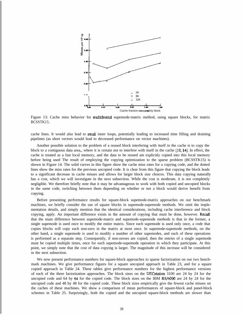
0.10t

z 2K9 8K2 32K

o%lo oio oio OAO OL A0Cache fraction occupmd by block

Figure 13: Cache miss behavior for multifrontal supemode-matrix method, using square blocks, for matrixBCSSTK15.

cache lines. It would also lead to sma.lI inner loops, potentially leading to increased time filling and drainingpipelines (as short vectors would lead to decreased performance on vector machines).

Another possible solution to the problem of a reused block interfering with itself in the cache is to copy theblock to a contiguous data area,, where it is certain not to interfere with itself in the cache [lo, 141. In effect, thecache is treated as a fast local memory, and the data to be reused am explicitly copied into this local memorybefore being used The result of employing the copying optimization to the sparse problem (BCSSTK15) isshown in Figure 14. The solid curves in this figure show the cache miss rates for a copying code, and the dottedlines show the miss rates for the previous uncopied code. It is clear from this figure that copying the block leadsto a significant decrease in cache misses and allows for larger block size choices. This data copying naturallyhas a cost, which we will investigate in the next subsection. While the cost is moderate, it is not completelynegligible. We therefore briefly note that it may be advantageous to work with both copied and uncopied blocksin the same code, switching between them depending on whether or not a block would derive benefit fromcopying.

Before presenting performance results for square-block supemode-matrix approaches on our benchmarkmachines, we briefly consider the use of square blocks in supemode-supemode methods. We omit the imple-mentation details, and simply mention that the identical considerations, including cache interference and blockcopying, apply. An important difference exists in the amount of copying that must be done, however. RecaIlthat the main difference between supemode-matrix and supemode-supemode methods is that in the former, asingle supemode is used once to modify the entire matrix. Since each supemode is used only once, a code thatcopies blocks will copy each non-zero in the matrix at most once. In supemode-supemode methods, on theother hand, a single supemode is used to modify a number of other supemodes, and each of these operationsis performed as a separate step. Consequently, if non-zeroes are copied, then the entries of a single supemodemust be copied multiple times, once for each supemode-supemode operation in which they participate. At thispoint, we simply note that the cost of data copying is larger. The magnitude of this increase will be consideredin the next subsection.

We now present performance numbers for square-block approaches to sparse factorization on our two bench-mark machines. We give performance figures for a square uncopied approach in Table 23, and for a squarecopied approach in Table 24. These tables give performance numbers for the highest performance versionsof each of the three factorization approaches. The block sizes on the DECstation 3100 are 24 by 24 for theuncopied code and 64 by 64 for the copied code. The block sizes on the IBM RS/6000 are 24 by 24 for theuncopied code and 48 by 48 for the copied code. These block sizes empirically give the fewest cache misses onthe caches of these machines. We show a comparison of mean performances of square-block and panel-blockschemes in Table 25. Surprisingly, both the copied and the uncopied square-block methods are slower than

38

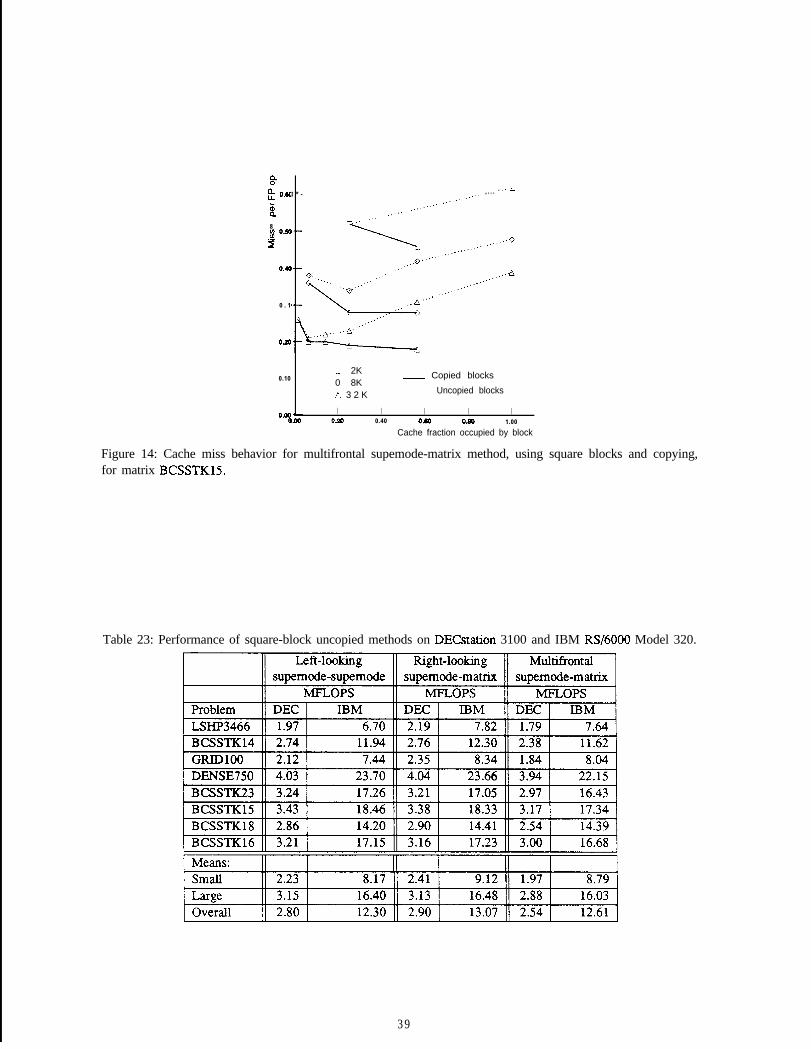
8-

k OM

zia

8v) 03

.(PI

0.40

0 . 1

OaO

0.10

O.os

. ..-zI * - , . . .

@..‘.,.....

,,.......’,..‘.

r 2K0 8K

- Copied blocks

c 3 2 K Uncopied blocks

I I I I I020 0.40 0.00 OdO 1.00

Cache fraction occupied by block

Figure 14: Cache miss behavior for multifrontal supemode-matrix method, using square blocks and copying,for matrix BCSSTK15.

Table 23: Performance of square-block uncopied methods on DECstation 3100 and IBM RS/6000 Model 320.

3 9

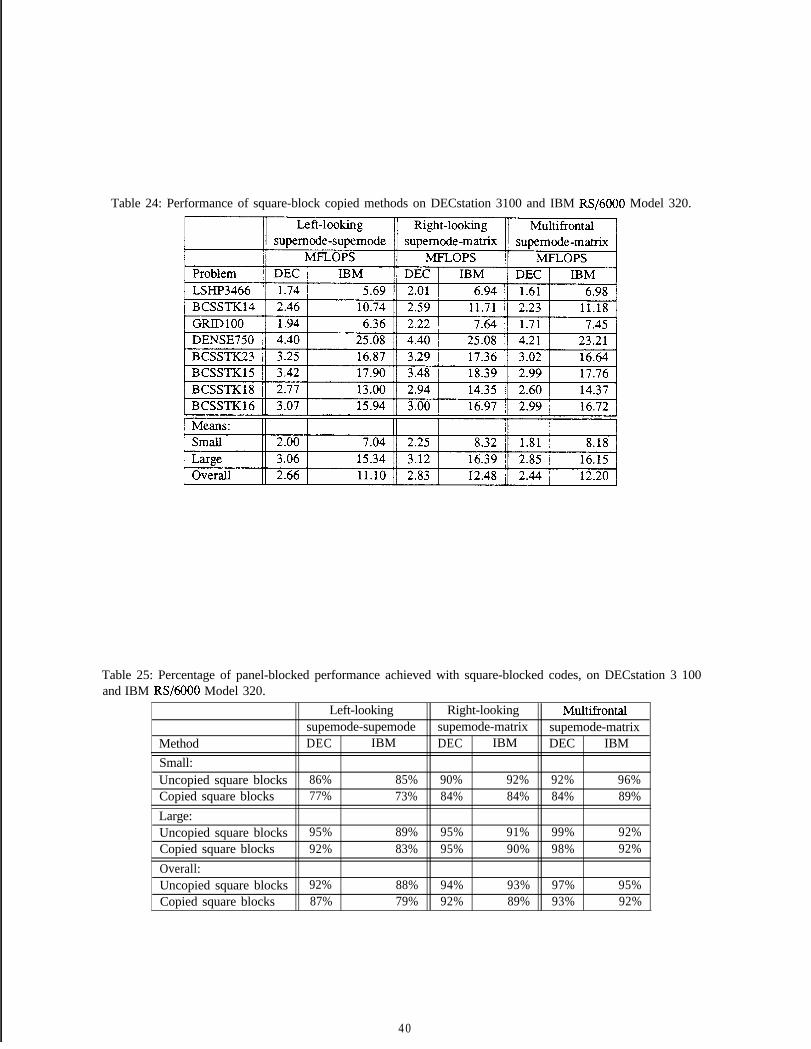
Table 24: Performance of square-block copied methods on DECstation 3100 and IBM RS/6000 Model 320.

Table 25: Percentage of panel-blocked performance achieved with square-blocked codes, on DECstation 3 100and IBM RS/6000 Model 320.

Left-looking Right-looking Multifrontalsupemode-supemode supemode-matrix supemode-matrix

Method DEC IBM DEC IBM DEC IBMSmall:Uncopied square blocks 86% 85% 90% 92% 92% 96%Copied square blocks 77% 73% 84% 84% 84% 89%Large:Uncopied square blocks 95% 89% 95% 91% 99% 92%Copied square blocks 92% 83% 95% 90% 98% 92%Overall:Uncopied square blocks 92% 88% 94% 93% 97% 95%Copied square blocks 87% 79% 92% 89% 93% 92%

4 0

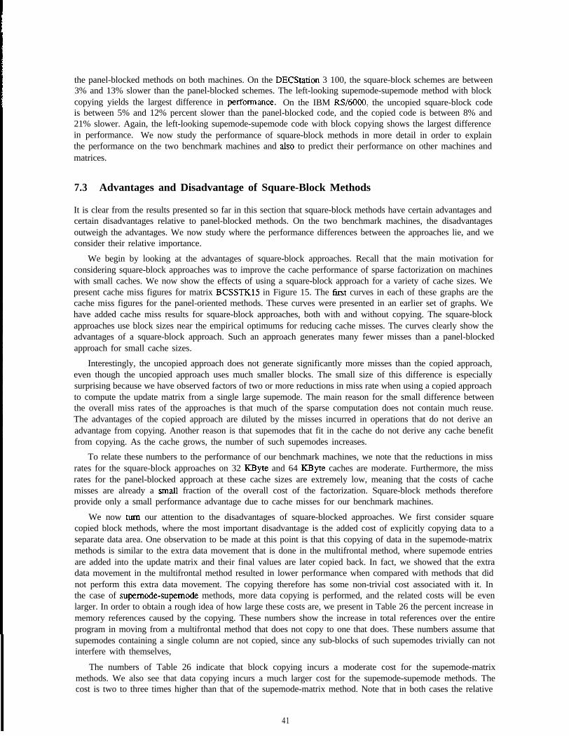
the panel-blocked methods on both machines. On the DECStation 3 100, the square-block schemes are between3% and 13% slower than the panel-blocked schemes. The left-looking supemode-supemode method with blockcopying yields the largest difference in pexfomance. On the IBM RS/60OO, the uncopied square-block codeis between 5% and 12% percent slower than the panel-blocked code, and the copied code is between 8% and21% slower. Again, the left-looking supemode-supemode code with block copying shows the largest differencein performance. We now study the performance of square-block methods in more detail in order to explainthe performance on the two benchmark machines and also to predict their performance on other machines andmatrices.

7.3 Advantages and Disadvantage of Square-Block Methods

It is clear from the results presented so far in this section that square-block methods have certain advantages andcertain disadvantages relative to panel-blocked methods. On the two benchmark machines, the disadvantagesoutweigh the advantages. We now study where the performance differences between the approaches lie, and weconsider their relative importance.

We begin by looking at the advantages of square-block approaches. Recall that the main motivation forconsidering square-block approaches was to improve the cache performance of sparse factorization on machineswith small caches. We now show the effects of using a square-block approach for a variety of cache sizes. Wepresent cache miss figures for matrix BCSSTK15 in Figure 15. The first curves in each of these graphs are thecache miss figures for the panel-oriented methods. These curves were presented in an earlier set of graphs. Wehave added cache miss results for square-block approaches, both with and without copying. The square-blockapproaches use block sizes near the empirical optimums for reducing cache misses. The curves clearly show theadvantages of a square-block approach. Such an approach generates many fewer misses than a panel-blockedapproach for small cache sizes.

Interestingly, the uncopied approach does not generate significantly more misses than the copied approach,even though the uncopied approach uses much smaller blocks. The small size of this difference is especiallysurprising because we have observed factors of two or more reductions in miss rate when using a copied approachto compute the update matrix from a single large supemode. The main reason for the small difference betweenthe overall miss rates of the approaches is that much of the sparse computation does not contain much reuse.The advantages of the copied approach are diluted by the misses incurred in operations that do not derive anadvantage from copying. Another reason is that supemodes that fit in the cache do not derive any cache benefitfrom copying. As the cache grows, the number of such supemodes increases.

To relate these numbers to the performance of our benchmark machines, we note that the reductions in missrates for the square-block approaches on 32 KByte and 64 KByte caches are moderate. Furthermore, the missrates for the panel-blocked approach at these cache sizes are extremely low, meaning that the costs of cachemisses are already a smaIl fraction of the overall cost of the factorization. Square-block methods thereforeprovide only a small performance advantage due to cache misses for our benchmark machines.

We now turn our attention to the disadvantages of square-blocked approaches. We first consider squarecopied block methods, where the most important disadvantage is the added cost of explicitly copying data to aseparate data area. One observation to be made at this point is that this copying of data in the supemode-matrixmethods is similar to the extra data movement that is done in the multifrontal method, where supemode entriesare added into the update matrix and their final values are later copied back. In fact, we showed that the extradata movement in the multifrontal method resulted in lower performance when compared with methods that didnot perform this extra data movement. The copying therefore has some non-trivial cost associated with it. Inthe case of supemode-supernode methods, more data copying is performed, and the related costs will be evenlarger. In order to obtain a rough idea of how large these costs are, we present in Table 26 the percent increase inmemory references caused by the copying. These numbers show the increase in total references over the entireprogram in moving from a multifrontal method that does not copy to one that does. These numbers assume thatsupemodes containing a single column are not copied, since any sub-blocks of such supemodes trivially can notinterfere with themselves,

The numbers of Table 26 indicate that block copying incurs a moderate cost for the supemode-matrixmethods. We also see that data copying incurs a much larger cost for the supemode-supemode methods. Thecost is two to three times higher than that of the supemode-matrix method. Note that in both cases the relative

41

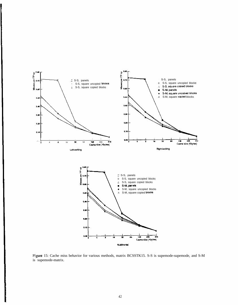
c S-S, panelso S-S, square uncopied blodcsA S-S, square copied blocks

z S-S, panelso S-S, square uncopied blocks

A S-M, square copled blocks

0.00 lI I I I I I I

I 22 4 6 16 s 64 126 266 212

Caohe she ( Bytes) Cache size (Kbytes)

Leftkddng Right hoking

5 S-S, panelso S-S, square uncopied blocksA S-S, square copied blocks

+ S-M, square uncopied blocksA S-M, square copied blocks

Cache size ( Wytee)

Figke 15: Cache miss behavior for various methods, matrix BCSSTK15. S-S is supemode-supemode, and S-Mis supemode-matrix.

42

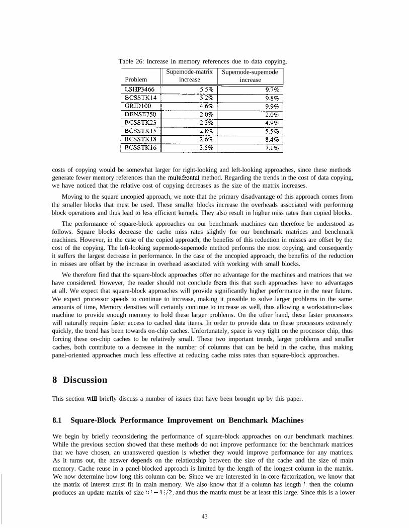
Table 26: Increase in memory references due to data copying.Supemode-matrix Supemode-supemode

Problem increase increase

costs of copying would be somewhat larger for right-looking and left-looking approaches, since these methodsgenerate fewer memory references than the multifrontal method. Regarding the trends in the cost of data copying,we have noticed that the relative cost of copying decreases as the size of the matrix increases.

Moving to the square uncopied approach, we note that the primary disadvantage of this approach comes fromthe smaller blocks that must be used. These smaller blocks increase the overheads associated with performingblock operations and thus lead to less efficient kernels. They also result in higher miss rates than copied blocks.

The performance of square-block approaches on our benchmark machines can therefore be understood asfollows. Square blocks decrease the cache miss rates slightly for our benchmark matrices and benchmarkmachines. However, in the case of the copied approach, the benefits of this reduction in misses are offset by thecost of the copying. The left-looking supemode-supemode method performs the most copying, and consequentlyit suffers the largest decrease in performance. In the case of the uncopied approach, the benefits of the reductionin misses are offset by the increase in overhead associated with working with small blocks.

We therefore find that the square-block approaches offer no advantage for the machines and matrices that wehave considered. However, the reader should not conclude from this that such approaches have no advantagesat all. We expect that square-block approaches will provide significantly higher performance in the near future.We expect processor speeds to continue to increase, making it possible to solve larger problems in the sameamounts of time, Memory densities will certainly continue to increase as well, thus allowing a workstation-classmachine to provide enough memory to hold these larger problems. On the other hand, these faster processorswill naturally require faster access to cached data items. In order to provide data to these processors extremelyquickly, the trend has been towards on-chip caches. Unfortunately, space is very tight on the processor chip, thusforcing these on-chip caches to be relatively small. These two important trends, larger problems and smallercaches, both contribute to a decrease in the number of columns that can be held in the cache, thus makingpanel-oriented approaches much less effective at reducing cache miss rates than square-block approaches.

8 Discussion

This section will briefly discuss a number of issues that have been brought up by this paper.

8.1 Square-Block Performance Improvement on Benchmark Machines

We begin by briefly reconsidering the performance of square-block approaches on our benchmark machines.While the previous section showed that these methods do not improve performance for the benchmark matricesthat we have chosen, an unanswered question is whether they would improve performance for any matrices.As it turns out, the answer depends on the relationship between the size of the cache and the size of mainmemory. Cache reuse in a panel-blocked approach is limited by the length of the longest column in the matrix.We now determine how long this column can be. Since we are interested in in-core factorization, we know thatthe matrix of interest must fit in main memory. We also know that if a column has length 1, then the columnproduces an update matrix of size I(1 + 1)/2, and thus the matrix must be at least this large. Since this is a lower

43

bound on the space required, and a dense matrix achieves this lower bound then the sparse matrix with thelongest columns that fits in a given amount of main memory is a dense matrix. If we consider our DECstation3100, which contains 64 KBytes of cache and 16 MBytes of main memory, a simple calculation reveals that thelargest dense matrix that fits in 16 MBytes is roughly 2000 by 2000. Since a 64 KByte cache fits 8 192 entries,at least four columns from this dense matrix, and thus from any matrix that fits in main memory, will fit incache. Thus, any problem that fits in main memory will achieve some degree of cache reuse on this machine.

If we consider the dense benchmark matrix (DENSE750), we note that at least 10 columns of this matrixfit in a 64K cache, and thus a panel-blocked method would use panels of that size. On the DECstation 3100, apanel-blocked method factored DENSE750 at a rate of 3.8 MFLOPS. The uncopied square-block method useda block size of 24, which would be expected to slightly increase reuse. indeed, the uncopied method factoredthe matrix at roughly 4.0 MFLOPS. The copied square-block method, with a block of size 64, significantlyincreases the amount of reuse and factors the matrix at a rate of 4.4 MFLOPS, or 16% faster.

A dense matrix provides only a lower bound on the number of columns that fit in the cache. A truly sparsematrix would have much shorter columns, so we would expect more reuse. For example, the largest 5-pointsquare grid problem that fits in 16 MBytes of memory is roughly 220 by 220. The longest column in thismatrix contains 330 entries, meaning that at least 24 columns would fit in the DECstation 3100 cache. Thus,for a machine with 64 KBytes of cache and 16MBytes of memory, we would expect a sparse matrix that fits inmain memory to achieve significant data reuse using a panel-blocked algorithm. Of course, a general-purposefactorization method should not make assumptions about the relative sizes of cache and main memory. We aresimply explaining the reasons for the lack of observed improvement, and pointing out that we would need amuch larger problem and much more memory to realize significant benefits from a square-block approach on amachine with such a large cache.

8.2 Improving Multifrontal Performance

Another question that we now consider is whether the performance disadvantage that the multifrontal methodsuffers relative to the other methods due to extra data movement can be overcome. Much of this extra datamovement is caused by the absence of a special case for handling supemodes that contain a single column.The problem of dealing with small supemodes in the multifrontal method has been recognized in the contextof vector supercomputers. One solution that has been investigated is supernode amalgamation [4, 93, wheresupemodes with similar structure are merged together to form larger supemodes. The cost of such merging is theintroduction of extra non-zeroes and extra floating-point operations. The merging is done selectively, so that thecosts associated with combining two supemodes are less than benefits derived Tom creating larger supernodes.Our observations about the lower performance of the multifrontal method on our benchmark machines indicatethat amalgamation techniques have a role in sparse factorization on workstation-class machines as well. Note,however, that the potential benefits of amalgamation are not specific to the multifrontal method. The performanceof the left-looking and right-looking approaches also suffers somewhat due to the existence of small supemodes,so we expect that amalgamation may benefit their performance as well.

Another possible means of improving the performance of the multifrontal method is through the introductionof a special case for single column supemodes. Briefly, one possible approach would be to ignore singletonsupemodes when they are visited in the tree traversal. When a non-singleton is visited, it would assemble allupdate matrices from the subtree rooted at itself in the elimination tree. If singletons were not ignored, then thesubtree update matrices would simply be the children’s update matrices. The values of the singleton supemodescould be computed during the assembly process, and similarly the updates from these singletons could be addeddirectly into the new update matrix. A special case like this is not nearly as clean as the special cases for theleft-looking and right-looking methods, however, and we have not further investigated such an approach.

.Yet another approach to improving the performance of the multifrontal method would be to use a hybridmethod, as suggested in [17]. Normally, the multifrontal method traverses the elimination tree all the way downto the leaves. Briefly, a multifrontal hybrid uses a multifrontal approach above certain nodes in the eliminationtree and an approach that is more efficient for small problems for the subtrees below those certain nodes. Theselection of the nodes at which the hybrid method would switch approaches would depend on the relativestrengths and wealmesses of the two blended approaches of the hybrid.

44

8.3 Choice of Primitives

Our study has considered a range of methods for factoring sparse matrices, including a number of methods thatare obviously non-optimal We have included such methods for a number of reasons. The first is to obtain abetter understanding of the benefits obtained by moving from one approach to another. In general, the methodsbased on higher-level primitives are much more complicated to implement. In particular, unrolling and blockingare quite tedious and time-consuming. We wanted to understand how much benefit was derived by expendingthe effort required to implement them. Also, through a gradual transition from relatively inefficient methodsto efficient methods, we were able to obtain an understanding of where the important sources performanceimprovement were.

Another reason for considering factorization primitives that are inefficient on hierarchical-memory machinesis that parallel factorization methods are typically implemented in terms of them. The reason has simply beenthat few distributed-hierarchical-memory multiprocessors have been available in the past. Since column-columnprimitives have no major disadvantages on machines without memory hierarchies, there was no reason not tobase parallel methods on them. This situation has been changing recently, however. As an example, the new InteliPSC/860 Touchstone multiprocessor is made up of a network of hierarchical-memory processors. Furthermore,we expect that most future high-performance parallel machines will be made up of collections of hierarchical-memory processors. By understanding the performance of column-column primitives on hierarchical-memorymachines, we can obtain a better understanding of how much the performance of these parallel approaches willsuffer due to the primitives they use.

Based on the results of this paper, it is clear that parallel methods implemented in terms of column-columnprimitives will achieve quite low performance on hierarchical-memory multiprocessors. However, we believethat the performance of these methods can be greatly improved. Specifically, we believe that these methods canachieve significantly higher performance by distributing sets of columns, or panels, among the processors ratherthan individual columns, as is typically done. A panel-oriented approach would allow higher-level primitivesto be used, yielding higher performance on each processor. We explored such an approach on a moderatelyparallel multiprocessor (an SGI 4D/380, 8 processor machine) in [20], with quite favorable results. However,a number of difficult questions remain to be answered. While higher-level primitives increase the efficiencyof the computations performed on each processor, they also dramatically decrease the amount of concurrencyin the problem, and thus decrease the number of processors that can effectively work on the problem at once.This decrease in concurrency was not a problem for the 8 processor machine with the matrices we considered,but it could conceivably become a problem on machines with larger numbers of processors. We are currentlyinvestigating this issue.

8.4 Performance Robustness

Our final point of discussion relates to the performance robustness of the methods that we have considered Whilethe relative performance levels of the fastest methods have been quite consistent across the different benchmarkmatrices on the machines that we have considered, it is quite possible that the methods have important weakpoints that were not brought out in the benchmark set.

The first thing to note when considering the robustness of factorization methods is that cache miss ratescan play an important role in determining performance. We therefore conclude that panel-blocked approachesare not robust. They generate significantly higher miss rates than square-blocked methods for large problemsor small caches, thus potentially resulting in significantly lower performance. A robust general-purpose codewould employ square-blocking. A similar but less important consideration is whether blocks should be copied.A copied code gives lower miss rates for small caches, but it also gives lower performance for small problemsdue to the cost of performing the actual copying. As was mentioned in the paper, a reasonable alternative isto use both approaches within the same code, switching between them on a per-supemode basis, depending onwhether copying would provide significant cache miss benefits for the current supemode.

Given the above considerations, we now consider the robustness of each method. Beginning with the left-looking supemode-supemode method, we note that this method contains a certain degree of unpredictability.When supemodes are copied, this method must perform more copying than the supemode-matrix methods.While the increase for the benchmark matrices we considered was moderate, there is no guarantee that it will

4 5

always be moderate. We can invent sparse matrices where supemode copying happens much more frequently.

The right-looking supemode-matrix method also contains some depe of uncertainty. This method mustcompute relative indices using an expensive search. While this search occurs extremely infrequently for thebenchmark matrices that we have considered, again there is no guarantee that it will not occur much morefrequently for other matrices. Also, the search code is likely to become even more expensive in the future, asthe amount of instruction parallelism that processors can exploit increases.

The multifrontal method provides the most robust performance among the three approaches. The cost ofcopying data in a copied square-block approach is guaranteed to be moderate, since each matrix entry is copied atmost once. The cost of computing relative indices is also moderate, since they are computed once per supemode.The performance of the multifrontal method on our benchmark machines was observed to be slightly lower thanthat of the other methods, but the difference was small. The multifrontal method contains some unpredictability,but it is not in the performance. Instead, the unpredictability is in the amount of space required to factor amatrix, since the size of the update matrix stack can vary widely.

9 Conclusions

An obvious end goal of a study like the one performed in this paper is to arrive at a particular choice of methodthat yields consistently higher performance than the other choices. Unfortunately, no factorization method fitthis description. Instead, a number of methods achieved roughly the same levels of performance, each with itsown advantages and disadvantages. A less ambitious goal for a general-purpose factorization method is that itprovide robust levels of performance, near the best performance of all other methods in almost all cases. Fromour discussion, it is clear that the multifrontal method best fits this description, although this method has thedisadvantages that it performs more data movement than other methods, it is more complicated to implement,and its storage requirements are larger and less predictable.

The primary conclusions we draw from this study relate less to which method is best overall and moreto what is required to achieve high performance with a sparse Cholesky factorization implementation. Ourconclusions are: (1) primitives that manipulate large structures are important for achieving high performance onhierarchical-memory machines; (2) the choice of left-looking, right-looking, or multifrontal approaches is lessimportant than the choice of the set of primitives on which to base them.

Acknowledgements

This research is supported by DARPA contract N00014-87-0828. Anoop Gupta is also supported by a PresidentialYoung Investigator award.

References

[l] Amestoy, P.R., and Duff, I.S., “Vector&&ion of a multiprocessor multifrontal code”, International Journalof Supercomputer Applications, 3 :41-59, 1989.

[2] Ashcraft, C.C., The domain/segment partition for the factorization of sparse symmetric positive definitematrices, Boeing Computer Services Technical Report ECA-TR-148, November, 1990.

[3] Ashcraft, C.C., A vector implementation of the multi’ontal method for large sparse symmetric positivedefinite linear systems, Boeing Computer Services Technical Report ETA-TR-5 1, May, 1987.

[4] Ashcraft, C.C., and Grimes, R.G., ‘The influence of relaxed supemode partitions on the multifrontalmethod”, ACM Transactions on Mathematical Software, 15(4): 291-309, 1989.

[5] Ashcraft, CC., Grimes, R.G., Lewis, J.G., Peyton, B.W., and Simon, H.D., “Recent progress in sparsematrix methods for large linear systems”, International Journal of Supercomputer Applications, I(4): 10-30,1987.

46

[6] Davis, H., Goldschmidt, S., and Hennessy, J., “Multiprocessing simulation and tracing using Tango”,Proceedings of the 1991 International Conference on Parallel Processing, August, 1991.

[7] Dongarra, J.J., and Eisenstat, S.C., “Squeezing the most out of an algorithm in CRAY FORTRAN”, ACMTransactions on Mathematical Sofhuare, lO(3); 219-230, 1984.

[8] Duff, I.S., Grimes, R.G., and Lewis, J.G., “Sparse Matrix Test Problems”, ACM Transactions on Mathe-matical Software, 15(l): 1-14, 1989.

[9] Duff, I.S., and Reid, J.K., “The multifrontal solution of indefinite sparse symmetric linear equations”, ACMTransactions on Mathematical Software, 9(3): 302-325, 1983.

[lo] GaIlivan, K., JaIby, W., Meier, U., and Sameh, A.H., “Impact of hierarchical memory systems on linearalgebra algorithm design”, International Journal of Supercomputer Applications, 2: 12-48, 1988.

[ll] George, A., Heath, M., Liu, J. and Ng, E., “Sparse Cholesky factorization on a local-memory multiproces-sor”, SIAM Journal on Scientifk and Statistical Computing’, 91327-340, 1988.

[12] George, A., and Liu, J., Computer Solution of Large Sparse Positive Definite Systems, Prentice-Hall, 1981.

[13] George, A., Liu, J., and Ng, E., User’s guide for SPARSPAK: Waterloo sparse linear equations package,Research Report CS-78-30, Department of Computer Science, University of Waterloo, 1980.

[14] Lam, M., Rothberg, E., and Wolf, M., ‘The Cache Performance and Optimizations of Blocked Algorithms”,Proceedings of the Fourth International Conference on Architectural Support for Programming Languagesand Operating Systems, April, 199 1.

[ 151 Liu, J., “Modification of the minimum degree algorithm by multiple elimination”, ACM Transactions onMathematical Sofiware, 12(2): 127-148, 1986.

[16] Liu, J., “On the storage requirement in the out-of-core multifrontal method for sparse factorization”, ACMTransactions on Mathematical Software, 12(3): 249-264, 1987.

[17] Liu, J., “The multifrontal method and paging in sparse Cholesky factorization”, ACM Transactions onMathematical Software, 15(4): 3 10-325, 1989.

[18] Ng, E.G., and Peyton, B.W., A supernodal Cholesky factorization algorithm for shared-memory multipro-cessors, Oak Ridge National Laboratory Technical Report ORNL/TM- 118 14, April, 1991.

[ 191 Rothberg, E., and Gupta, A., “Efficient Sparse Matrix Factorization on Hierarchical Memory Workstations- Exploiting the Memory Hierarchy”, to appear in ACM Transactions on Mathematical Software.

[20] Rothberg, E., and Gupta, A., “Techniques for improving the performance of sparse matrix factorization onmultiprocessor workstations”, Supercomputing ‘90, p. 232-243 , November, 1990.

[21] Schreiber, R., “A new implementation of sparse Gaussian elimination”, ACM Transactions on MathematicalSoftware, 8~256276, 1982.

4 7