Embed Size (px)
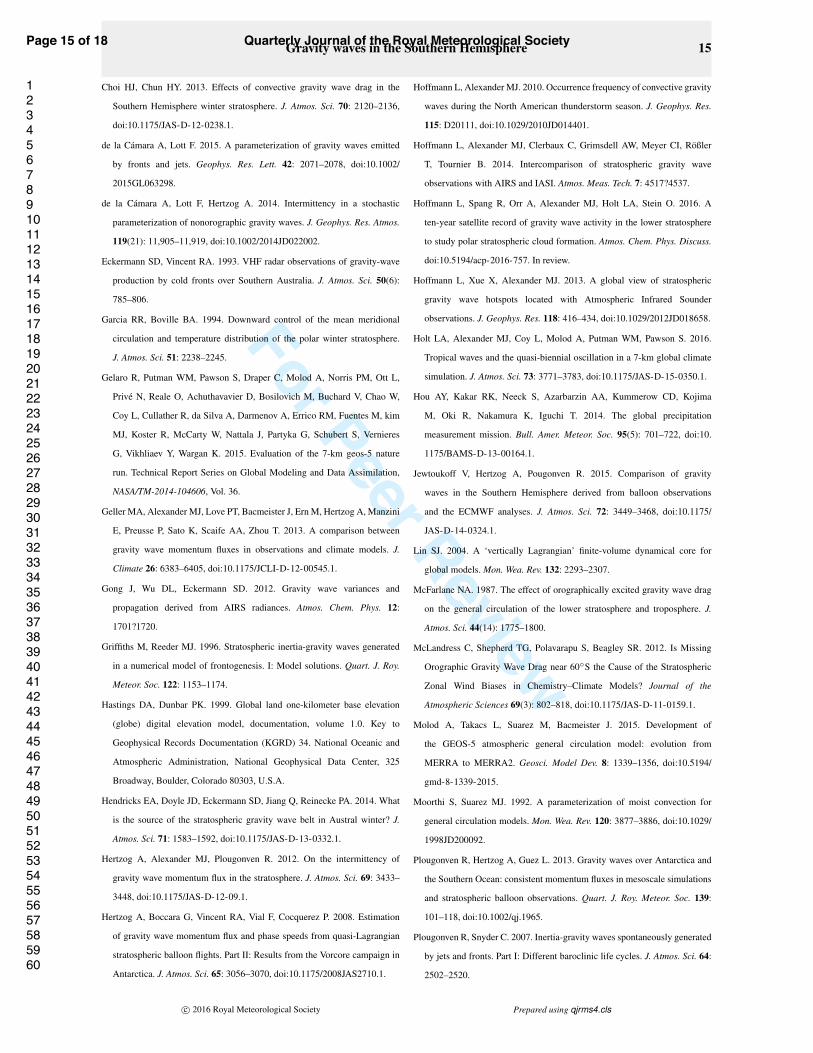
Citation preview
For Peer Review
Gravity waves in the Southern Hemisphere 1
An evaluation of gravity waves and their sources in the Southern
Hemisphere in a 7-km global climate simulation
L. A. Holta∗, M. J. Alexandera, L. Coyb,c, C. Liue, A. Molodb, W. Putmanb, and S. Pawsonb
aNorthWest Research Associates, 3380 Mitchell Lane, Boulder, CO 80301
bGlobal Modeling and Assimilation Office, NASA Goddard Space Flight Center, Greenbelt, Maryland
cScience Systems and Applications Inc, Lanham, Maryland
eDepartment of Physical and Environmental Sciences, Texas A&M University-Corpus Christi, Corpus Christi, Texas
∗Correspondence to: Laura A. Holt, NorthWest Research Associates, 3380 Mitchell Lane, Boulder, CO 80301.
Email: [email protected]
In this study, gravity waves in the high-resolution GEOS-5 Nature Run are first
evaluated with respect to satellite and other model results. Southern Hemisphere
winter sources of nonorographic gravity waves in the model are then investigated by
linking measures of tropospheric nonorographic gravity wave generation with absolute
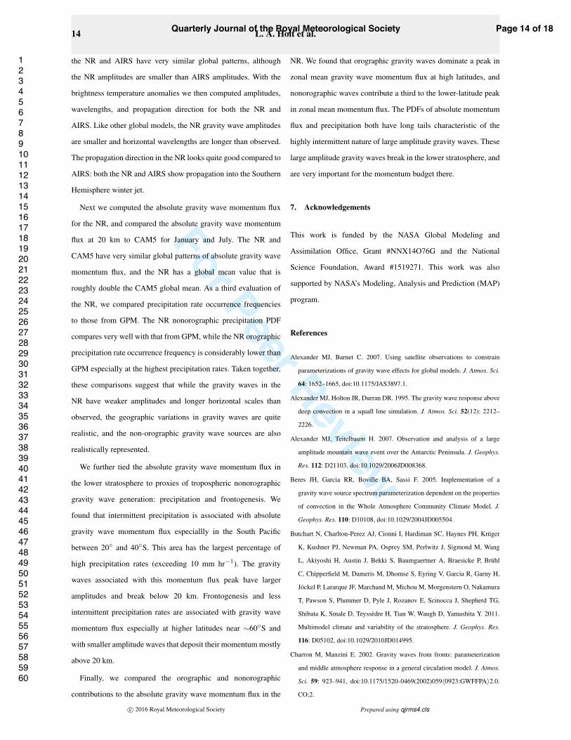
gravity wave momentum flux in the lower stratosphere. Finally, nonorographic gravity
wave momentum flux is compared to orographic gravity wave momentum flux and
compared to previous estimates. The results show that the global patterns in gravity
wave amplitude, horizontal wavelength, and propagation direction are very realistic
compared to observations. However, like other global models the amplitudes are weaker
and horizontal wavelengths longer than observed. The global patterns in absolute
gravity wave momentum flux also agree well with previous model and observational
estimates. The evaluation of model nonorographic gravity wave sources in the Southern
Hemisphere winter shows that strong intermittent precipitation (greater than 10 mm
per hr) is associated with gravity wave momentum flux over the South Pacific, and
frontogenesis and less intermittent, lower precipitation rates (less than 10 mm per hr)
are associated with gravity wave momentum flux near 60 degrees S. In the model,
orographic gravity waves contribute almost exclusively to a peak in zonal mean
momentum flux between 70 and 75 degrees S, while nonorographic waves dominate
at 60 degrees S, and nonorographic gravity waves contribute a third to a peak in zonal
mean momentum flux between 25 and 30 degrees S.
Key Words: gravity waves, gravity wave sources, nonorographic gravity waves, Southern Hemisphere, gravity wave
momentum flux, high-resolution climate simulation
c⃝ 2016 Royal Meteorological Society Prepared using qjrms4.cls
Page 1 of 18 Quarterly Journal of the Royal Meteorological Society
123456789101112131415161718192021222324252627282930313233343536373839404142434445464748495051525354555657585960
For Peer Review
Quarterly Journal of the Royal Meteorological Society Q. J. R. Meteorol. Soc. 00: 2–16 (2016)
1. Introduction
Gravity waves are important drivers of circulation and transport
in the middle atmosphere. They are currently included in most
climate models via parameterizations due to computational
limitations on resolution. The resolution required to resolve
the full gravity wave spectrum is orders of magnitude higher
than is employed by current climate models, which means that
climate models will need to rely on gravy wave parameterizations
for the foreseeable future. However, at this time gravity wave
parameterizations remain poorly constrained by observations.
This contributes to large model biases in middle atmosphere
temperatures and winds, especially in the Southern Hemisphere
stratosphere (Butchart et al. 2011; McLandress et al. 2012).
Some studies show improvements in model biases when gravity
wave parameterizations are tied to tropospheric sources of gravity
wave generation (Beres et al. 2005; Charron and Manzini 2002;
Song and Chun 2005; Richter et al. 2010). For example, Choi and
Chun (2013) showed that wind biases in the Southern Hemisphere
winter stratosphere were reduced in a global climate model
when they included a convective gravity wave parameterization in
addition to the existing gravity wave drag parameterization. Other
studies have shown better model realism when the gravity wave
parameterization is based on an intermittent source function (de la
Camara and Lott 2015). This is based on several papers that have
shown the highly intermittent nature of gravity wave generation,
both in observations and models (e.g., Hertzog et al. 2008, 2012;
Jewtoukoff et al. 2015; Plougonven et al. 2013).
The main sources of gravity waves are orography, jets/fronts,
and convection. It is generally thought that the distributions of
these sources vary with latitude, with convection dominating in
the Tropics and jets, fronts, and orography dominating in the
midlatitudes (Plougonven and Zhang 2014). Orographic gravity
wave momentum fluxes are typically several times larger than
nonorographic gravity wave momentum flux and are concentrated
over orographic features (e.g., Vincent et al. 2007; Hertzog et al.
2008; Jewtoukoff et al. 2015). Even though orographic gravity
wave momentum fluxes are much larger than nonorographic
gravity wave momentum fluxes locally, nonorographic gravity
waves have been shown to contribute substantially to the total
gravity wave momentum flux since they are generated over a
much larger area (Hertzog et al. 2008). Convection is an important
generation mechanism of nonorographic gravity waves in the
troposphere (e.g., Alexander et al. 1995), and the importance
of moisture has been highlighted in idealized models (Wei and
Zhang 2014). Fronts are also known to be a major source of
nonorographic gravity waves (Eckermann and Vincent 1993;
Plougonven and Snyder 2007). However, the relative importance
of different nonorographic gravity wave sources is still not
completely understood.
This study examines gravity waves and their sources, with
an emphasis on the Southern Hemisphere winter, in a 7-km
horizontal resolution global climate model. Global models in
general, and the model used in this study in particular, are good
tools for this investigation because they have complete winds and
temperatures output on a regular grid and high-resolution that
resolves much of the gravity wave spectrum. We first validate the
gravity wave properties and global distributions with respect to
observations and other models. Then we examine the relationship
between nonorographic gravity waves and sources. Finally we
compare orographic and nonorographic gravity wave momentum
flux.
The paper is organized as follows. In Section 2 we describe
the model. In Section 3 we validate the model’s gravity waves
by first comparing them to those observed by the Atmospheric
Infrared Sounder (AIRS) and then computing the January and
July absolute gravity wave momentum flux and comparing it to
previous model estimates. In Section 4 we relate the absolute
gravity wave momentum flux in the lower stratosphere to proxies
of tropospheric wave generation. In Section 5 we compare the
momentum fluxes generated by orographic gravity waves to those
generated by nonorographic gravity waves. Finally, we provide a
summary and closing remarks in Section 6.
2. GEOS-5 Nature Run
The Nature Run (NR) is a global non-hydrostatic, 7-km horizontal
resolution mesoscale simulation produced by the Goddard Earth
Observing System (GEOS-5) atmospheric general circulation
model (Gelaro et al. 2015; Putman et al. 2014) with finite-
volume (FV) dynamics (based on Lin (2004)) on a cubed-sphere
c⃝ 2016 Royal Meteorological Society Prepared using qjrms4.cls
Page 2 of 18Quarterly Journal of the Royal Meteorological Society
123456789101112131415161718192021222324252627282930313233343536373839404142434445464748495051525354555657585960
For Peer Review
Gravity waves in the Southern Hemisphere 3
horizontal grid (Putman and Lin 2007). The NR simulation
was run for roughly 2 years, from May 2005 to June 2007,
with 72 vertical levels from the surface up to ∼0.01 hPa (∼85
km). The vertical resolution is ∼200 m or less below 800 hPa,
∼500 m near 600 hPa, ∼1 km near the tropopause, and ∼2
km near the stratopause. The physics, remapping, and dynamics
time steps were 300, 75, and 5 s, respectively. The NR was
forced with prescribed sea-surface temperature and sea-ice at
0.25◦ resolution, biomass burning emissions (organic and black
carbon aerosols, SO2, CO, and CO2) at 0.1◦ resolution, and
anthropogenic emissions (aerosols, CO, CO2, SO2, SO4) at 0.1◦
resolution (for details see Putman et al. 2014).
The NR is in the “gray zone” of atmospheric model resolution,
where the resolution is high enough to start resolving smaller-
scale processes like convection but not high enough to resolve
them completely. Models in the gray zone still need to rely on
parameterizations to some degree, but these parameterizations can
be relaxed compared to coarser resolution models. Convection in
GEOS-5 is parameterized using the Relaxed Arakawa-Schubert
(RAS) scheme of Moorthi and Suarez (1992). As resolution
increases, the RAS is controlled by a stochastic limit on deep
convection (Tokioka et al. 1988), which basically confines the
RAS to function as a shallow convection scheme. Another
resolution-aware parameterization in GEOS-5 is the orographic
gravity wave parameterization (McFarlane 1987). Parameterized
orographic waves are forced by sub-grid scale variance, which is
scaled down with increasing resolution to account for the increase
in resolved waves produced by the dynamics of the model.
Even with a very high horizontal resolution, the NR still
required a non-orographic gravity wave parameterization (based
on Garcia and Boville 1994) to achieve realistic gravity wave
drag and circulation in the middle atmosphere. Holt et al. (2016)
discussed this issue in depth for the tropics and concluded that
non-orographic gravity wave generation was realistic in the NR
but that the non-orographic gravity wave parameterization was
necessary because the waves were too heavily dissipated by the
model. The NR included explicit diffusion from second-order
divergence damping, which provided a strong damping on the
resolved gravity waves. Parameterized non-orographic gravity
waves were specified with an equatorial peak in momentum flux
(see Figure 3 in Molod et al. (2015)), and the phase speed
spectrum was launched from 400 hPa with a range of ±40 m s−1
in increments of 10 m s−1.
For the analysis of the NR in this paper, we used 30-minute
instantaneous output that was interpolated from the cubed-sphere
grid to a 0.0625◦ × 0.0625◦ (lon × lat) grid while maintaining the
full model vertical grid. We also used hourly instantaneous output
interpolated to 0.5◦ × 0.5◦ (lon × lat) horizontal resolution also
maintaining the full model vertical grid.
3. Validation of the gravity waves in the NR
3.1. Comparison to AIRS
The AIRS instrument on NASA’s Aqua satellite provides global
coverage of infrared radiance spectra in three spectral bands
between 3.74 and 15.4 µm. The 4.3 and 15 µm CO2 bands
have been used extensively to study gravity waves in the
stratosphere (e.g., Alexander and Teitelbaum 2007; Gong et al.
2012; Hoffmann et al. 2013, 2014, 2016). Here we use the AIRS
4.3 µm channel average brightness temperatures described in
Hoffmann and Alexander (2010). AIRS uses cross-track scanning,
where each scan consists of 90 footprints over 1780 km (at the
ground) and is separated by 18 km along-track distance. The
footprint size varies with the scanning angle between 14×14 km2
and 21×42 km2 (see Figure 2 in Hoffmann et al. (2014)).
To obtain AIRS brightness temperature anomalies, background
variations first need to be removed. Additionally, AIRS raw
radiances have a limb-brightening in the cross-track direction that
needs to be removed before studying the small-scale waves. As
is traditionally done with AIRS, a fourth-order polynomial fit
in the x-direction was used to remove the background at each
y-location, where the x-direction refers to cross-track scanning
and the y-direction refers to along-track scanning. In addition to
removing the limb-brightening effect, this method removes larger-
scale wave perturbations with horizontal wavelengths longer
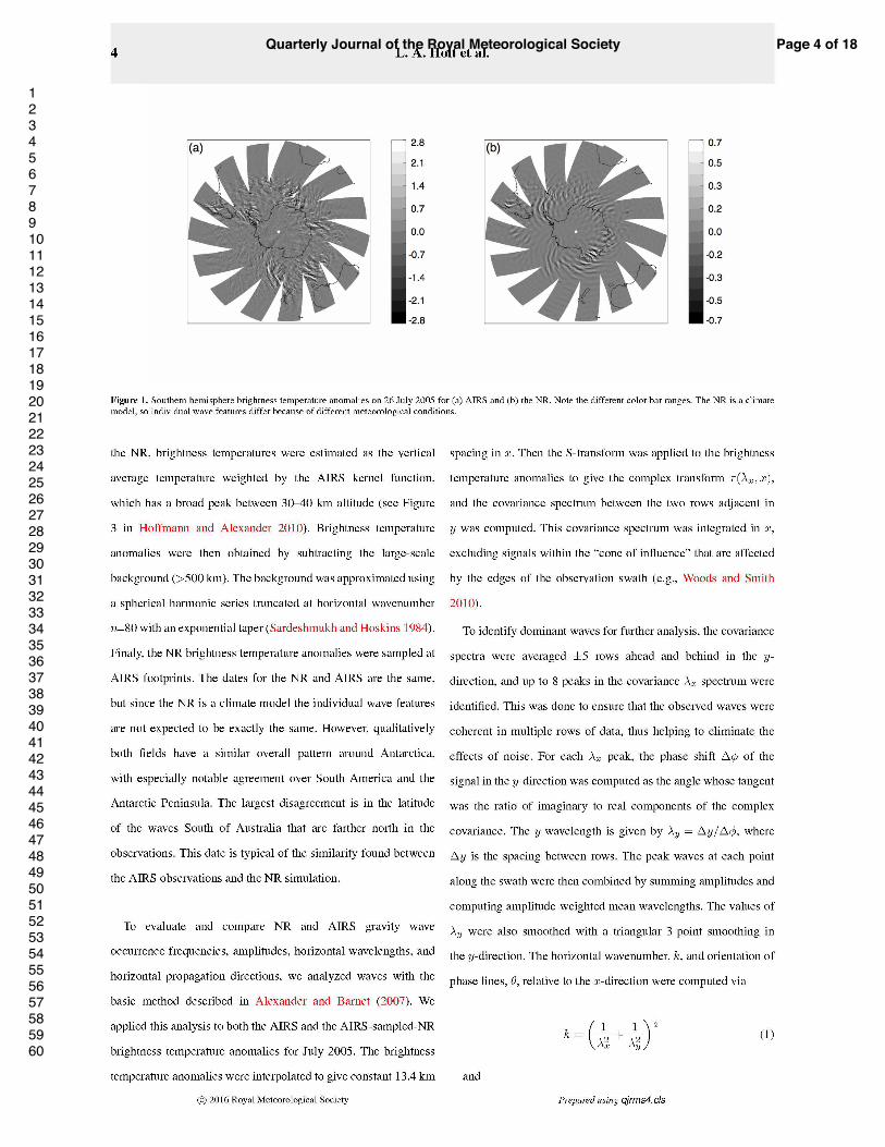
than ∼500 km. Figure 1 shows an example of the AIRS
brightness temperature anomalies on 26 July 2005 in the Southern
Hemisphere.
Figure 1 also shows NR brightness temperature anomalies
sampled at the AIRS measurement locations for the same day. For
c⃝ 2016 Royal Meteorological Society Prepared using qjrms4.cls
Page 3 of 18 Quarterly Journal of the Royal Meteorological Society
123456789101112131415161718192021222324252627282930313233343536373839404142434445464748495051525354555657585960
For Peer Review
Page 4 of 18Quarterly Journal of the Royal Meteorological Society
123456789101112131415161718192021222324252627282930313233343536373839404142434445464748495051525354555657585960
For Peer Review
Page 5 of 18 Quarterly Journal of the Royal Meteorological Society
123456789101112131415161718192021222324252627282930313233343536373839404142434445464748495051525354555657585960
For Peer Review
Page 6 of 18Quarterly Journal of the Royal Meteorological Society
123456789101112131415161718192021222324252627282930313233343536373839404142434445464748495051525354555657585960
For Peer Review
Gravity waves in the Southern Hemisphere 7
et al. (2013), which was the first international collaborative
effort at direct comparisons of global gravity wave momentum
fluxes in observations and models. Because satellite methods
only permitted estimates of the absolute values of momentum
flux with no knowledge of direction, similar estimates of
absolute momentum flux were computed and compared. Some
of the models were high resolution, permitting an analysis
of the resolved gravity waves. Others were coarse resolution,
so the gravity wave fluxes were obtained from the model
parameterizations of gravity wave drag.
We estimated the absolute gravity wave momentum flux for
resolved waves in the NR using wind and temperature quadratics
(u′2, v′2, w′2, T ′2) as in Equation (1) in Geller et al. (2013):
M2=
!
1−f2
ω2
"
ρ20
#
$
u′w′%2
+$
v′w′%2&
= ρ20w′2'
u′2 + v′2(
)
1−f2
ω2
* )
1 +f2
ω2
*
(3)
where
f2
ω2=
f2g2T ′2
w′2N4T 20
. (4)
T0 and ρ0 are large-scale temperature and density, respectively.
N is the Brunt–Vaisala frequency, f is the Coriolis parameter, ω
is the gravity wave intrinsic frequency, and g is Earth’s gravity.
Primes denote variations smaller than this large scale, which is
taken to be 1000 km. The large-scale was approximated by a
spherical harmonic series truncated at horizontal wavenumber
n=40 with an exponential taper. The overbars denote averages
over 10◦ longitude × 5◦ latitude geographical bins. The terms
in brackets on the right-hand side of Equation 3 represent a low-
frequency correction. However, the correction only changed the
global mean absolute gravity wave momentum flux by less than
3%.
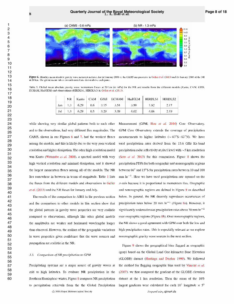
Figure 6 shows the absolute gravity wave momentum flux at
∼20 km for January 2006 of the NR and also for January 2006 of
the CAM5 run presented in Geller et al. (2013) for comparison.
Two CAM5 experiments were initialized on 1 June 2005 and
run at ∼0.25◦ horizontal resolution with observed sea-surface
temperatures for 18 months. Figure 6 shows the average of the
two CAM5 runs. The absolute gravity wave momentum fluxes
for CAM5 were calculated with Equation 3 (Equation 1 from
Geller et al. (2013)). The NR and CAM5 have very similar global
patterns of absolute gravity wave momentum flux. In particular,
both models have maxima over topographic features in the winter
hemisphere. In the NR the largest maximum is over the Rocky
Mountains, whereas the largest maximum in CAM5 is over the
Tibetan Plateau. The global mean values are also shown at the top
of the panel for both models. The NR global mean value is double
the CAM5 global mean value. The NR has roughly four times the
horizontal resolution of the CAM5 simulation. The global mean
momentum fluxes in the NR are between 2.4 and 3 times weaker
than parameterized gravity waves in the coarse resolution models
in the Geller et al. (2013) comparison.
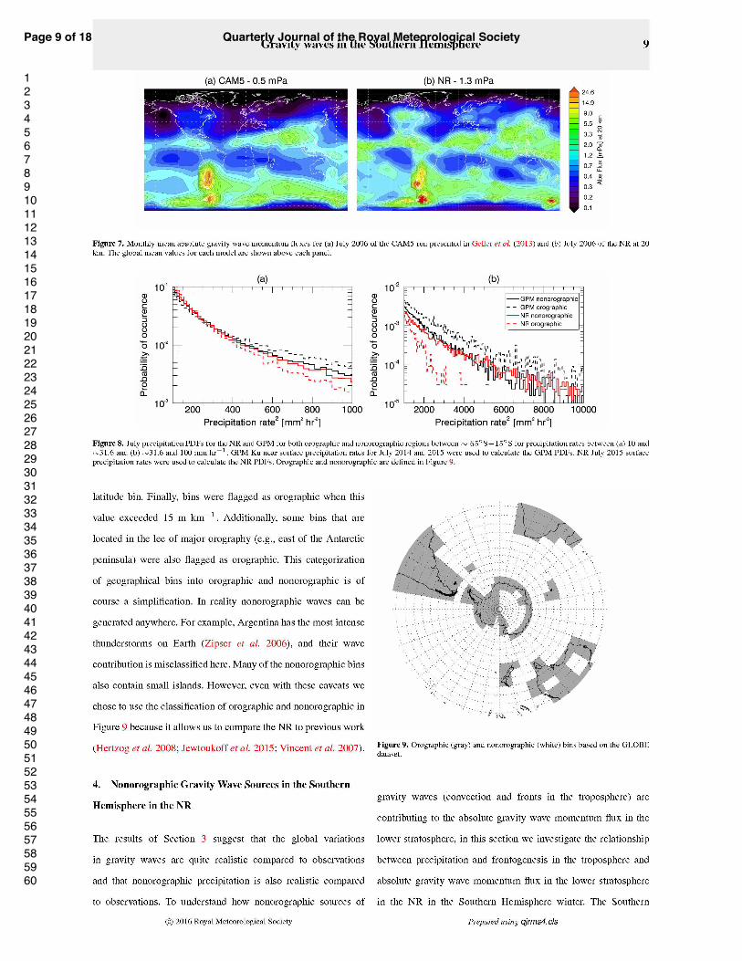
Figure 7 shows the absolute gravity wave momentum flux at
∼20 km for July 2006 of the NR and also for July 2006 of the
CAM5 run presented in Geller et al. (2013) for comparison. As for
January, the NR and CAM5 have very similar global patterns of
absolute gravity wave momentum flux. In the winter hemisphere,
both the NR and CAM5 have orographic maxima over the
Antarctic Peninsula and the southern tip of South America. Both
also show a large area of nonorographic flux over the Southern
Ocean and into the Indian, South Atlantic, and South Pacific
Oceans. In the summer hemisphere, the patterns of secondary
maxima agree remarkably well.
The Geller et al. (2013) results showed large disparities
among different observational estimates of the flux, and large
differences between observations and models, which spoke to
the remaining large uncertainty in the observational estimates.
However, one surprising result was how similar three different
climate models with six (two each, orographic and non-
orographic) different gravity wave parameterization methods all
showed rather similar gravity wave momentum fluxes. Since
the different parameterization methods had all been tuned to
give realistic simulations of the general circulation, perhaps in
hindsight this result should not have been surprising. On the
other hand, the resolved waves in two high-resolution models,
c⃝ 2016 Royal Meteorological Society Prepared using qjrms4.cls
Page 7 of 18 Quarterly Journal of the Royal Meteorological Society
123456789101112131415161718192021222324252627282930313233343536373839404142434445464748495051525354555657585960
For Peer Review
Page 8 of 18Quarterly Journal of the Royal Meteorological Society
123456789101112131415161718192021222324252627282930313233343536373839404142434445464748495051525354555657585960
For Peer Review
Page 9 of 18 Quarterly Journal of the Royal Meteorological Society
123456789101112131415161718192021222324252627282930313233343536373839404142434445464748495051525354555657585960
For Peer Review
10 L. A. Holt et al.
Hemisphere winter stratosphere is the locus of larger than average
climate model biases in wind and temperature (Butchart et al.
2011; McLandress et al. 2012) with important implications for
modeling ozone chemistry. Because of limited land areas, the
Southern Hemisphere is also a region of particular interest in
understanding nonorographic gravity wave sources (Hertzog et al.
2008; de la Camara et al. 2014).
Although the validation in Section 3 showed the total fluxes in
the NR are likely weaker than in nature, the realism of a model like
the NR with resolved sources and waves permits an examination
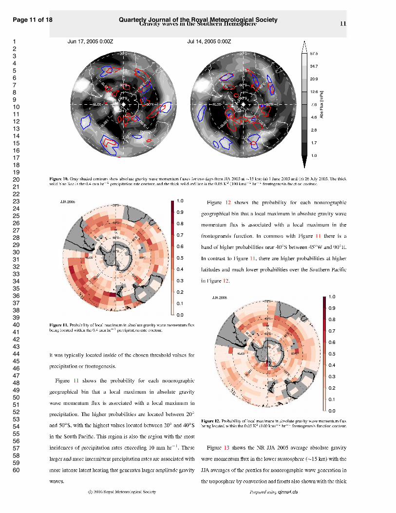
of the relative contributions of different sources. Figure 10 shows
absolute gravity wave momentum flux in the lower stratosphere
(∼15 km) for two Southern Hemisphere winter days in 2005 with
proxies for nonorographic wave generation in the troposphere
by convection and fronts. We chose precipitation rate and the
frontogenesis function as our indicators of tropospheric wave
generation. Precipitation rates are related to the strength and depth
of moist convection, which is an important generation mechanism
of gravity waves in the troposphere (e.g., Alexander et al. 1995).
Fronts are also known to be a major source of gravity waves
(Eckermann and Vincent 1993; Plougonven and Snyder 2007).
The absolute gravity wave momentum flux near 15 km was
computed as before with Equation 3 and binned to 10◦ longitude
× 5◦ latitude. For the precipitation rate, we averaged the 0.0625◦
surface precipitation in each 10◦ longitude × 5◦ latitude bin.
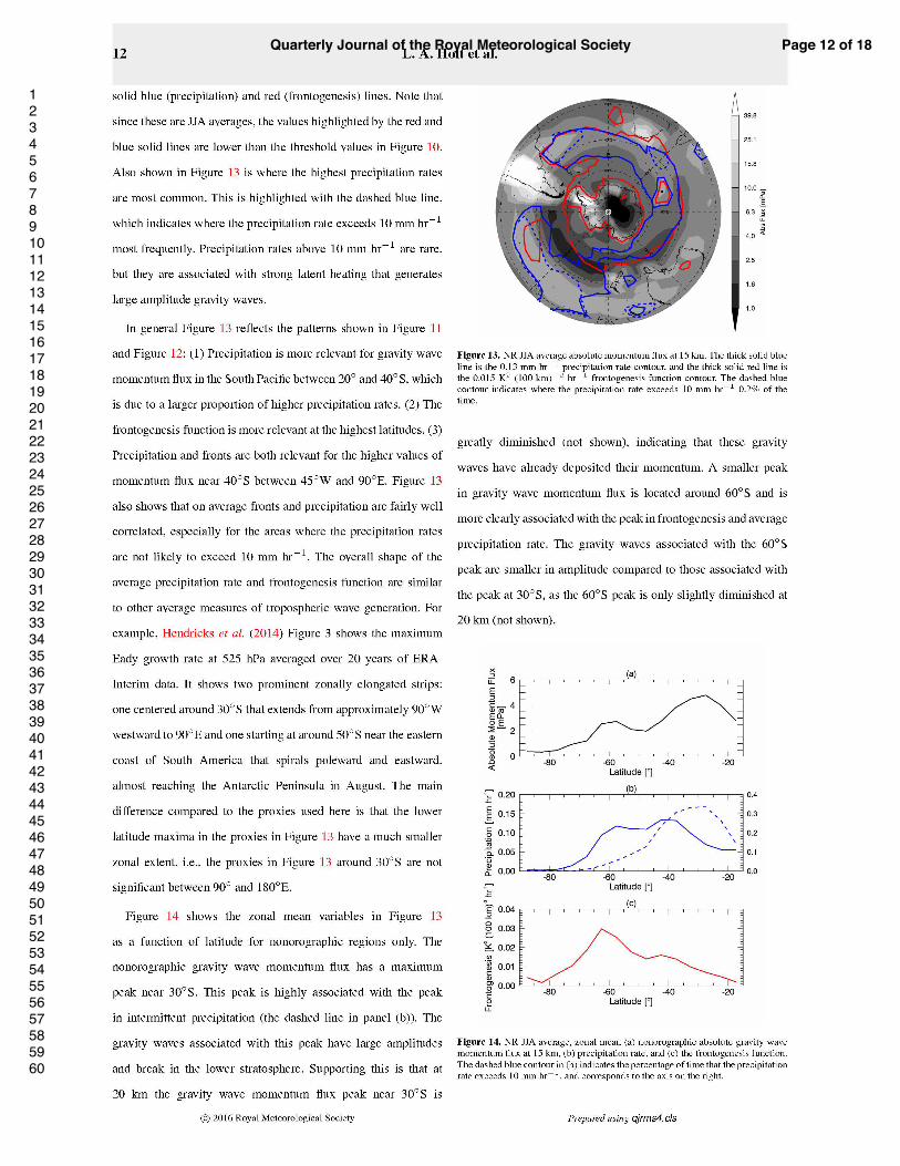
The precipitation threshold shown in Figure 10 with the thick
blue contour is 0.4 mm hr−1. The threshold is only shown for
nonorographic regions (as defined in Figure 9). The frontogenesis
function at ∼800 hPa was computed via Equation 2.1 in Charron
and Manzini (2002):
1
2
D|∇θ|2
Dt=−
!
1
a cosφ
∂θ
∂λ
"2 )
1
a cosφ
∂u
∂λ−
v tanφ
a
*
−
!
1
a
∂θ
∂φ
"2 )
1
a
∂v
∂φ
*
−
!
1
a cos θ
∂θ
∂λ
"
×
)
1
a cosφ
∂v
∂λ+
1
a
∂u
∂φ+
u tanφ
a
*
(5)
where θ is potential temperature, u is the zonal wind, v is the
meridional wind, λ is longitude, and φ is latitude, and θ, u, and
v are the large-scale fields (>1000 km here). The large-scale θ, u,
and v were approximated by a spherical harmonic series truncated
at horizontal wavenumber n=40 with an exponential taper. Since
only coarse resolution fields were needed for the calculation, we
used the 0.5◦ variables for this calculation. After the frontogenesis
function was computed, it was binned to 10◦ longitude × 5◦
latitude. Gravity wave parameterizations that tie gravity waves
to sources via frontogenesis use a threshold value, and gravity
waves are launched when the frontogenesis function exceeds the
threshold. The value is typically somewhere between 0.045 and
0.1 K2 (100 km)−2 hr−1 (Griffiths and Reeder 1996; Charron and
Manzini 2002; Richter et al. 2010). We chose a conservative value
of 0.05 K2 (100 km)−2 hr−1, which is shown in Figure 10 with
the thick red contours for nonorographic regions.
In general the gravity wave momentum flux maxima are located
inside the blue and red contours (areas with high precipitation
and frontogenesis). Sometimes the precipitation and frontogenesis
maxima coincide, but this is not always the case. The precipitation
maxima are located predominantly between 20◦ and 40◦S, and
the frontogenesis maxima are mostly located at the higher
latitudes. To evaluate the relationship between absolute gravity
wave momentum flux in the lower stratosphere and precipitation
and frontogenesis in the troposphere, we flagged a geographical
bin each time a momentum flux maxima was located inside
the threshold values for precipitation or frontogenesis. We did
this for each day in JJA 2005 with hourly variables. Then for
each bin we added up the number of flags and divided by
the total number of time steps. The resulting probabilities are
shown for precipitation in Figure 11 and for frontogenesis in
Figure 12. We chose this method over a simple correlation
with each geographical bin because maxima in precipitation and
frontogenesis were usually not in the exact same geographical bin
as a maximum in momentum flux. This is because gravity waves
propagate horizontally in addition to propagating vertically. We
found that while a momentum flux maximum was usually not
precisely colocated with preciptiation or frontogenesis maxima,
c⃝ 2016 Royal Meteorological Society Prepared using qjrms4.cls
Page 10 of 18Quarterly Journal of the Royal Meteorological Society
123456789101112131415161718192021222324252627282930313233343536373839404142434445464748495051525354555657585960
For Peer Review
Page 11 of 18 Quarterly Journal of the Royal Meteorological Society
123456789101112131415161718192021222324252627282930313233343536373839404142434445464748495051525354555657585960
For Peer Review
Page 12 of 18Quarterly Journal of the Royal Meteorological Society
123456789101112131415161718192021222324252627282930313233343536373839404142434445464748495051525354555657585960
For Peer Review
Page 13 of 18 Quarterly Journal of the Royal Meteorological Society
123456789101112131415161718192021222324252627282930313233343536373839404142434445464748495051525354555657585960
For Peer Review
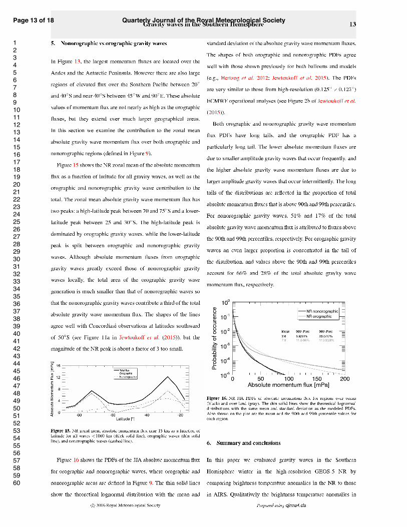
14 L. A. Holt et al.
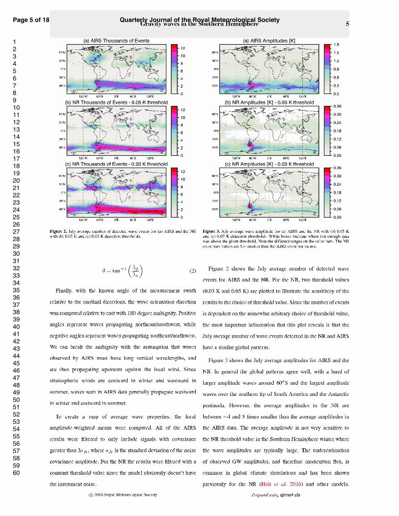
the NR and AIRS have very similar global patterns, although
the NR amplitudes are smaller than AIRS amplitudes. With the
brightness temperature anomalies we then computed amplitudes,
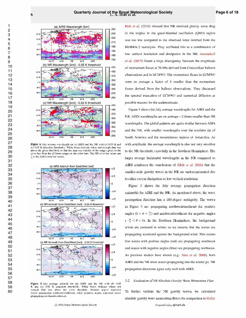
wavelengths, and propagation direction for both the NR and
AIRS. Like other global models, the NR gravity wave amplitudes
are smaller and horizontal wavelengths are longer than observed.
The propagation direction in the NR looks quite good compared to
AIRS: both the NR and AIRS show propagation into the Southern
Hemisphere winter jet.
Next we computed the absolute gravity wave momentum flux
for the NR, and compared the absolute gravity wave momentum
flux at 20 km to CAM5 for January and July. The NR and
CAM5 have very similar global patterns of absolute gravity wave
momentum flux, and the NR has a global mean value that is
roughly double the CAM5 global mean. As a third evaluation of
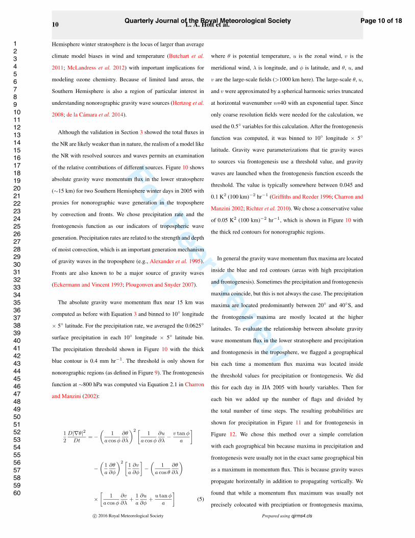
the NR, we compared precipitation rate occurrence frequencies
to those from GPM. The NR nonorographic precipitation PDF
compares very well with that from GPM, while the NR orographic
precipitation rate occurrence frequency is considerably lower than
GPM especially at the highest precipitation rates. Taken together,
these comparisons suggest that while the gravity waves in the
NR have weaker amplitudes and longer horizontal scales than
observed, the geographic variations in gravity waves are quite
realistic, and the non-orographic gravity wave sources are also
realistically represented.
We further tied the absolute gravity wave momentum flux in
the lower stratosphere to proxies of tropospheric nonorographic
gravity wave generation: precipitation and frontogenesis. We
found that intermittent precipitation is associated with absolute
gravity wave momentum flux especiallly in the South Pacific
between 20◦ and 40◦S. This area has the largest percentage of
high precipitation rates (exceeding 10 mm hr−1). The gravity
waves associated with this momentum flux peak have larger
amplitudes and break below 20 km. Frontogenesis and less
intermittent precipitation rates are associated with gravity wave
momentum flux especially at higher latitudes near ∼60◦S and
with smaller amplitude waves that deposit their momentum mostly
above 20 km.
Finally, we compared the orographic and nonorographic
contributions to the absolute gravity wave momentum flux in the
NR. We found that orographic gravity waves dominate a peak in
zonal mean gravity wave momentum flux at high latitudes, and
nonorographic waves contribute a third to the lower-latitude peak
in zonal mean momentum flux. The PDFs of absolute momentum
flux and precipitation both have long tails characteristic of the
highly intermittent nature of large amplitude gravity waves. These
large amplitude gravity waves break in the lower stratosphere, and
are very important for the momentum budget there.
7. Acknowledgements
This work is funded by the NASA Global Modeling and
Assimilation Office, Grant #NNX14O76G and the National
Science Foundation, Award #1519271. This work was also
supported by NASA’s Modeling, Analysis and Prediction (MAP)
program.
References
Alexander MJ, Barnet C. 2007. Using satellite observations to constrain
parameterizations of gravity wave effects for global models. J. Atmos. Sci.
64: 1652–1665, doi:10.1175/JAS3897.1.
Alexander MJ, Holton JR, Durran DR. 1995. The gravity wave response above
deep convection in a squall line simulation. J. Atmos. Sci. 52(12): 2212–
2226.
Alexander MJ, Teitelbaum H. 2007. Observation and analysis of a large
amplitude mountain wave event over the Antarctic Peninsula. J. Geophys.
Res. 112: D21103, doi:10.1029/2006JD008368.
Beres JH, Garcia RR, Boville BA, Sassi F. 2005. Implementation of a
gravity wave source spectrum parameterization dependent on the properties
of convection in the Whole Atmosphere Community Climate Model. J.
Geophys. Res. 110: D10108, doi:10.1029/2004JD005504.
Butchart N, Charlton-Perez AJ, Cionni I, Hardiman SC, Haynes PH, Kruger
K, Kushner PJ, Newman PA, Osprey SM, Perlwitz J, Sigmond M, Wang
L, Akiyoshi H, Austin J, Bekki S, Baumgaertner A, Braesicke P, Bruhl
C, Chipperfield M, Dameris M, Dhomse S, Eyring V, Garcia R, Garny H,
Jockel P, Lararque JF, Marchand M, Michou M, Morgenstern O, Nakamura
T, Pawson S, Plummer D, Pyle J, Rozanov E, Scinocca J, Shepherd TG,
Shibata K, Smale D, Teyssedre H, Tian W, Waugh D, Yamashita Y. 2011.
Multimodel climate and variability of the stratosphere. J. Geophys. Res.
116: D05102, doi:10.1029/2010JD014995.
Charron M, Manzini E. 2002. Gravity waves from fronts: parameterization
and middle atmosphere response in a general circulation model. J. Atmos.
Sci. 59: 923–941, doi:10.1175/1520-0469(2002)059⟨0923:GWFFPA⟩2.0.
CO;2.
c⃝ 2016 Royal Meteorological Society Prepared using qjrms4.cls
Page 14 of 18Quarterly Journal of the Royal Meteorological Society
123456789101112131415161718192021222324252627282930313233343536373839404142434445464748495051525354555657585960
For Peer Review
Gravity waves in the Southern Hemisphere 15
Choi HJ, Chun HY. 2013. Effects of convective gravity wave drag in the
Southern Hemisphere winter stratosphere. J. Atmos. Sci. 70: 2120–2136,
doi:10.1175/JAS-D-12-0238.1.
de la Camara A, Lott F. 2015. A parameterization of gravity waves emitted
by fronts and jets. Geophys. Res. Lett. 42: 2071–2078, doi:10.1002/
2015GL063298.
de la Camara A, Lott F, Hertzog A. 2014. Intermittency in a stochastic
parameterization of nonorographic gravity waves. J. Geophys. Res. Atmos.
119(21): 11,905–11,919, doi:10.1002/2014JD022002.
Eckermann SD, Vincent RA. 1993. VHF radar observations of gravity-wave
production by cold fronts over Southern Australia. J. Atmos. Sci. 50(6):
785–806.
Garcia RR, Boville BA. 1994. Downward control of the mean meridional
circulation and temperature distribution of the polar winter stratosphere.
J. Atmos. Sci. 51: 2238–2245.
Gelaro R, Putman WM, Pawson S, Draper C, Molod A, Norris PM, Ott L,
Prive N, Reale O, Achuthavavier D, Bosilovich M, Buchard V, Chao W,
Coy L, Cullather R, da Silva A, Darmenov A, Errico RM, Fuentes M, kim
MJ, Koster R, McCarty W, Nattala J, Partyka G, Schubert S, Vernieres
G, Vikhliaev Y, Wargan K. 2015. Evaluation of the 7-km geos-5 nature
run. Technical Report Series on Global Modeling and Data Assimilation,
NASA/TM-2014-104606, Vol. 36.
Geller MA, Alexander MJ, Love PT, Bacmeister J, Ern M, Hertzog A, Manzini
E, Preusse P, Sato K, Scaife AA, Zhou T. 2013. A comparison between
gravity wave momentum fluxes in observations and climate models. J.
Climate 26: 6383–6405, doi:10.1175/JCLI-D-12-00545.1.
Gong J, Wu DL, Eckermann SD. 2012. Gravity wave variances and
propagation derived from AIRS radiances. Atmos. Chem. Phys. 12:
1701?1720.
Griffiths M, Reeder MJ. 1996. Stratospheric inertia-gravity waves generated
in a numerical model of frontogenesis. I: Model solutions. Quart. J. Roy.
Meteor. Soc. 122: 1153–1174.
Hastings DA, Dunbar PK. 1999. Global land one-kilometer base elevation
(globe) digital elevation model, documentation, volume 1.0. Key to
Geophysical Records Documentation (KGRD) 34. National Oceanic and
Atmospheric Administration, National Geophysical Data Center, 325
Broadway, Boulder, Colorado 80303, U.S.A.
Hendricks EA, Doyle JD, Eckermann SD, Jiang Q, Reinecke PA. 2014. What
is the source of the stratospheric gravity wave belt in Austral winter? J.
Atmos. Sci. 71: 1583–1592, doi:10.1175/JAS-D-13-0332.1.
Hertzog A, Alexander MJ, Plougonven R. 2012. On the intermittency of
gravity wave momentum flux in the stratosphere. J. Atmos. Sci. 69: 3433–
3448, doi:10.1175/JAS-D-12-09.1.
Hertzog A, Boccara G, Vincent RA, Vial F, Cocquerez P. 2008. Estimation
of gravity wave momentum flux and phase speeds from quasi-Lagrangian
stratospheric balloon flights. Part II: Results from the Vorcore campaign in
Antarctica. J. Atmos. Sci. 65: 3056–3070, doi:10.1175/2008JAS2710.1.
Hoffmann L, Alexander MJ. 2010. Occurrence frequency of convective gravity
waves during the North American thunderstorm season. J. Geophys. Res.
115: D20111, doi:10.1029/2010JD014401.
Hoffmann L, Alexander MJ, Clerbaux C, Grimsdell AW, Meyer CI, Roßler
T, Tournier B. 2014. Intercomparison of stratospheric gravity wave
observations with AIRS and IASI. Atmos. Meas. Tech. 7: 4517?4537.
Hoffmann L, Spang R, Orr A, Alexander MJ, Holt LA, Stein O. 2016. A
ten-year satellite record of gravity wave activity in the lower stratosphere
to study polar stratospheric cloud formation. Atmos. Chem. Phys. Discuss.
doi:10.5194/acp-2016-757. In review.
Hoffmann L, Xue X, Alexander MJ. 2013. A global view of stratospheric
gravity wave hotspots located with Atmospheric Infrared Sounder
observations. J. Geophys. Res. 118: 416–434, doi:10.1029/2012JD018658.
Holt LA, Alexander MJ, Coy L, Molod A, Putman WM, Pawson S. 2016.
Tropical waves and the quasi-biennial oscillation in a 7-km global climate
simulation. J. Atmos. Sci. 73: 3771–3783, doi:10.1175/JAS-D-15-0350.1.
Hou AY, Kakar RK, Neeck S, Azarbarzin AA, Kummerow CD, Kojima
M, Oki R, Nakamura K, Iguchi T. 2014. The global precipitation
measurement mission. Bull. Amer. Meteor. Soc. 95(5): 701–722, doi:10.
1175/BAMS-D-13-00164.1.
Jewtoukoff V, Hertzog A, Pougonven R. 2015. Comparison of gravity
waves in the Southern Hemisphere derived from balloon observations
and the ECMWF analyses. J. Atmos. Sci. 72: 3449–3468, doi:10.1175/
JAS-D-14-0324.1.
Lin SJ. 2004. A ‘vertically Lagrangian’ finite-volume dynamical core for
global models. Mon. Wea. Rev. 132: 2293–2307.
McFarlane NA. 1987. The effect of orographically excited gravity wave drag
on the general circulation of the lower stratosphere and troposphere. J.
Atmos. Sci. 44(14): 1775–1800.
McLandress C, Shepherd TG, Polavarapu S, Beagley SR. 2012. Is Missing
Orographic Gravity Wave Drag near 60◦S the Cause of the Stratospheric
Zonal Wind Biases in Chemistry–Climate Models? Journal of the
Atmospheric Sciences 69(3): 802–818, doi:10.1175/JAS-D-11-0159.1.
Molod A, Takacs L, Suarez M, Bacmeister J. 2015. Development of
the GEOS-5 atmospheric general circulation model: evolution from
MERRA to MERRA2. Geosci. Model Dev. 8: 1339–1356, doi:10.5194/
gmd-8-1339-2015.
Moorthi S, Suarez MJ. 1992. A parameterization of moist convection for
general circulation models. Mon. Wea. Rev. 120: 3877–3886, doi:10.1029/
1998JD200092.
Plougonven R, Hertzog A, Guez L. 2013. Gravity waves over Antarctica and
the Southern Ocean: consistent momentum fluxes in mesoscale simulations
and stratospheric balloon observations. Quart. J. Roy. Meteor. Soc. 139:
101–118, doi:10.1002/qj.1965.
Plougonven R, Snyder C. 2007. Inertia-gravity waves spontaneously generated
by jets and fronts. Part I: Different baroclinic life cycles. J. Atmos. Sci. 64:
2502–2520.
c⃝ 2016 Royal Meteorological Society Prepared using qjrms4.cls
Page 15 of 18 Quarterly Journal of the Royal Meteorological Society
123456789101112131415161718192021222324252627282930313233343536373839404142434445464748495051525354555657585960
For Peer Review
16 L. A. Holt et al.
Plougonven R, Zhang F. 2014. Internal gravity waves from atmospheric jets
and fronts. Rev. Geophys. 52: 33–76, doi:10.1002/2012RG000419.
Putman WM, da Silva AM, Ott L, Darmenov A. 2014. Model configuration
for the 7-km GEOS-5.12 Nature Run, Ganymed Release (Non-hydrostatic
7 km Global Mesoscale Simulation). GMAO Office Note No. 5.0 (Version
1.0), 18 pp., available from http://gmao.gsfc.nasa.gov/pubs/office notes.
Putman WM, Lin SJ. 2007. Finite-volume transport on various cubed-sphere
grids. J. Computat. Phys. 227: 55–78.
Richter JH, Sassi F, Garcia RR. 2010. Toward a physically based gravity wave
source parameterization in a general circulation model. J. Atmos. Sci. 67:
136–156, doi:10.1175/2009JAS3112.1.
Sardeshmukh PD, Hoskins BJ. 1984. Spatial smoothing on the sphere. Mon.
Wea. Rev. 112: 2524–2529.
Sato K, Watanabe S, Kawatani Y, Tomikawa Y, Miyazaki K, Takahashi M.
2009. On the origins of mesospheric gravity waves. Geophys. Res. Lett. 36:
L19801, doi:10.1029/2009GL039908.
Seto S, Iguchi T, Oki T. 2013. The basic performance of a precipitation
retrieval algorithm for the global precipitation measurement mission’s
single/dual-frequency radar measurements. IEEE Trans. Geosci. Remote
Sens. 51(12): 5239–5251, doi:10.1109/TGRS.2012.2231686.
Song IS, Chun HY. 2005. Momentum flux spectrum of convectively
forced internal gravity waves and its application to gravity wave drag
parameterization. Part I: Theory. J. Atmos. Sci. 62: 107–124, doi:10.1175/
JAS-3363.1.
Tokioka T, Yamazaki K, Kitoh A, Ose T. 1988. The equatorial
30?60 day oscillation and the Arakawa-Schubert penetrative cumulus
parameterization. J. Meteor. Soc. Japan 66: 883–901.
Vincent RA, Hertzog A, Boccara G, Vial F. 2007. Quasi-Lagrangian
superpressure balloon measurements of gravity-wave momentum fluxes in
the polar stratosphere of both hemispheres. Geophys. Res. Lett. 34: L19804,
doi:10.1029/2007GL031072.
Watanabe S, Kawatani Y, Tomikawa Y, Miyazaki K, Takahashi M,
Sato K. 2008. General aspects of a T213L256 middle atmosphere
general circulation model. J. Geophys. Res. 113: D12110, doi:10.1029/
2008JD010026.
Wei J, Zhang F. 2014. Mesoscale gravity waves in moist baroclinic jet-front
systems. J. Atmos. Sci. 71: 929–952, doi:10.1175/JAS-D-13-0171.1.
Woods BK, Smith RB. 2010. Energy flux and wavelet diagnostics of secondary
mountain waves. J. Atmos. Sci. 67: 3721–3738, doi:10.1175/2009JAS3285.
1.
Zipser E, Liu C, D C, Nesbitt SW, Yorty S. 2006. Where are the most intense
thunderstorms on Earth? Bull. Amer. Meteor. Soc. 87: 1057–1071.
c⃝ 2016 Royal Meteorological Society Prepared using qjrms4.cls
Page 16 of 18Quarterly Journal of the Royal Meteorological Society
123456789101112131415161718192021222324252627282930313233343536373839404142434445464748495051525354555657585960