Embed Size (px)
Citation preview
An Evaluation of Employee Performance
Based on Imprecise Value Judgments Two Experiments
STIG BLOMSKOG
WORKING PAPER 2007:2
SÖ
DE
RT
ÖR
NS
HÖ
GS
KO
LA
(UN
IVE
RS
ITY
CO
LL
EG
E)
2007-04-02
An evaluation of employee performance
based on imprecise value judgments:
Two experiments*
Stig Blomskog
Södertörn University College
Box 4101 Huddinge
SE-141 89 Sweden
E-mail: [email protected]
Tel : +46(0)8 608 40 52
Fax : +46(0)8 608 44 80
* I wish to thank professor Ahti Salo at the Systems Analysis Laboratory, Helsinki University of Technology, for constructive comments. I also wish to thank Christine Bladh, Department Chair of History at Södertörn University College, for her participation in the experiments. This study has been funded by the Swedish Council for Working Life and Social Research.
1(36)
Abstract
In this paper we test the usefulness of imprecise value judgments in evaluating
employee performance. The test is based on two experiments which evaluate the
performance of college lecturers. The experiments are carried out by applying the
PRIME model (Preference Ratios in Multi-attribute Evaluation), a specific multi-
attribute value model that supports the use of imprecise value judgments. The test shows
that the use of imprecise value judgments, as synthesized by the PRIME model, can
remedy a number of defects that are identified in conventional evaluation models in
regard to job requirements and employee performance.
KEY WORDS: employee performance; imprecise value judgments; salary
compensation
2(36)
1. Introduction
Job requirements and employee performance are usually evaluated on the basis of a
complex aggregate of those criteria and attributes considered relevant to a rational
structure of salary compensation. The complexity of this evaluation is often increased
by its being based on the assessment of criteria and attributes that lack a precise
definition – something that adds a degree of subjectivity to the process. Assessments of
an employee’s relative degree of responsibility or social competence are typical
examples of such vague criteria. In spite of this, many frequently used and conventional
models for evaluating employee performance and job requirements not only utilize
obviously fuzzy, vague value judgments, but also present these in the guise of precise
numerical quantities. This gives the impression that the basic value judgments possess
much greater precision than is in fact the case. The resultant job and employee-
performance evaluation presents numerical information whose precision is, in fact,
artificial and arbitrary. It gives, therefore, a biased presentation of the imprecise value
judgments that form its base. This false precision obfuscates the link between the value
judgments upon which the evaluation rests and the evaluation results. This is an
unsatisfactory situation, especially as increases in non-standardized jobs and
individualized systems of salary compensation have led to an increased use of this type
of employee evaluation (Lazear, 1998; Kira, 2000). Furthermore, many Equal Pay Acts
support the use of job evaluation in order to investigate salary discrimination by gender.
A possible way to remedy this problematic situation is to use evaluation models that
support the use of imprecise or vague value judgments.
The aim of this paper is to test the usefulness of applying a specific multi-attribute
value model, termed PRIME (Preference Ratios in Multi-attribute Evaluation), that
supports the use of imprecise value judgments in evaluating employee performance. The
test is carried out as two experiments that evaluate the performance of a restricted
number of academic lecturers at Södertörn University College. The imprecise and basic
value judgments are modeled by numerical intervals, the length of which represents the
relative degree of imprecision of value judgments. The software, PRIME Decisions, can
be downloaded from: www.hut.fi\Units\SAL\Downloadables\ (Salo and Hämäläinen,
2001; Gustafsson et al, 2000).
As far as we know the PRIME model has not been applied in the context of
evaluation of jobs and employee performance. Therefore we decided to delimit the
3(36)
experiments in several respects in order to make a first test more tractable. In the first
place, the evaluation of lecturer performance is restricted to a subset of those criteria
considered relevant for salary compensation at Södertörn University College. Secondly,
the paper does not address many important questions of principles concerning the
relation between individualized salary compensation and employee performance –
questions such as: What principles should be applied for choosing relevant criteria and
for evaluating employee performance? Who should develop such principles? How
should the evaluation procedure be organized? and so on. Discussion of such issues
should only occur, most appropriately, once the test of the PRIME model supporting
imprecise value judgments and its thorough introduction to the decision makers have
been completed. These delimitations mean of course that results of the evaluations
carried out in the experiments cannot be used without further development in an actual
salary setting process. Instead the value of the experiments is to gather experience from
using evaluation models such as PRIME that support the use of imprecise value
judgments. Such experience is an important basis for the further development of
methods, which gives rise to more reliable evaluation of jobs and of employee
performance.
The paper is organized as follows. The next section offers a brief description and a
critical analysis of a conventional evaluation method, here termed the “point rating”
model. This method, which is often used to evaluate job requirements and employee
performance, is recommended by the European Project on Equal Pay, which is
supported by European Commission (Harriman & Holm 2001). The third section
introduces the PRIME model. The fourth section presents the two experiments and ends
with a comparison of the PRIME- and the “point rating”- models. The fifth section
concludes the paper with a final discussion of the superiority of the PRIME model.
2. A conventional evaluation method
The “point rating” model defines an evaluation process as follows:
1) The decision maker (here abbreviated as DM) defines a set of relevant criteria: nk CCCC ,.....,,........, 21 kC = criterion k 2) Each criterion is then divided into a number of category-levels:
kjk CL ∈
4(36)
jkL = jth level of criterion k
3) The DM ranks the levels:
max min... ...jk kL L kL
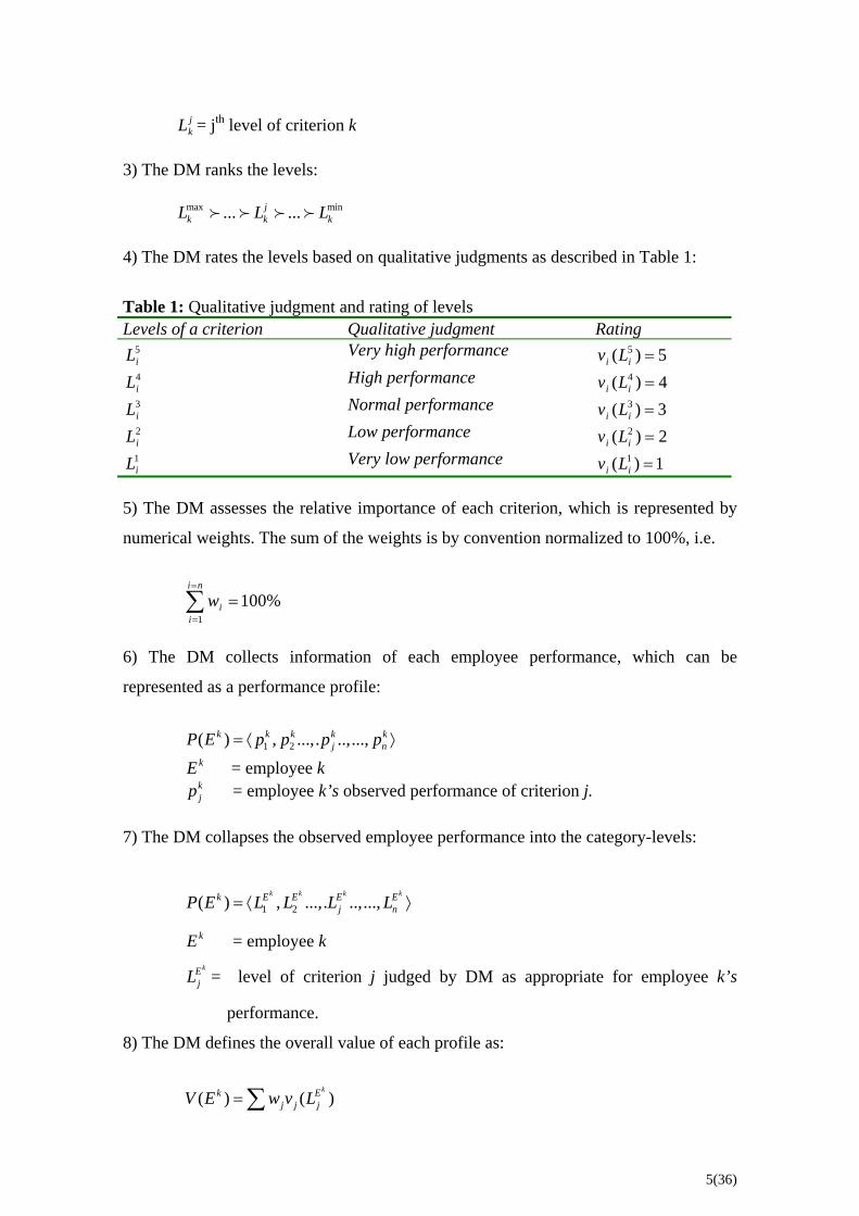
4) The DM rates the levels based on qualitative judgments as described in Table 1:
Table 1: Qualitative judgment and rating of levels Levels of a criterion Qualitative judgment Rating
5iL Very high performance 5)( 5 =ii Lv4iL High performance 4)( 4 =ii Lv 3iL Normal performance 3)( 3 =ii Lv 2iL Low performance 2)( 2 =ii Lv 1iL Very low performance 1)( 1 =ii Lv
5) The DM assesses the relative importance of each criterion, which is represented by
numerical weights. The sum of the weights is by convention normalized to 100%, i.e.
%1001
=∑=
=
ni
iiw
6) The DM collects information of each employee performance, which can be
represented as a performance profile:
1 2( ) , ...,. ..,...,k k k k
j nP E p p p p= ⟨ ⟩k kE = employee k kjp = employee k’s observed performance of criterion j.
7) The DM collapses the observed employee performance into the category-levels:
1 2( ) , ...,. ..,...,k k k kk E E E E
j nP E L L L L= ⟨ ⟩
kE = employee k kE
jL = level of criterion j judged by DM as appropriate for employee k’s
performance.
8) The DM defines the overall value of each profile as:
( ) (
kk Ej j jV E w v L=∑ )
5(36)
where =jw relative weight of criterion j
( )kE
j jv L = rating of level kE
jL
9) The DM ranks employees based on the overall value of each performance profile.
lk EE if and only if ( )kE
j j jw v L∑ > (lE
j j jw v L )∑ lk EE ~ if and only if =)(
kEjjj Lvw∑ (
lEj j jw v L )∑
Thus the ranking of employees is based on an additive value model specified by precise
numerical information regarding weights and value functions. The ranking’s reliability
and stability is questionable, however, because no justification is given for representing
the value judgment as precise numerical information. This questionable translation of
value judgments into precise numerical information is especially noticeable in steps 4, 5
and 7.
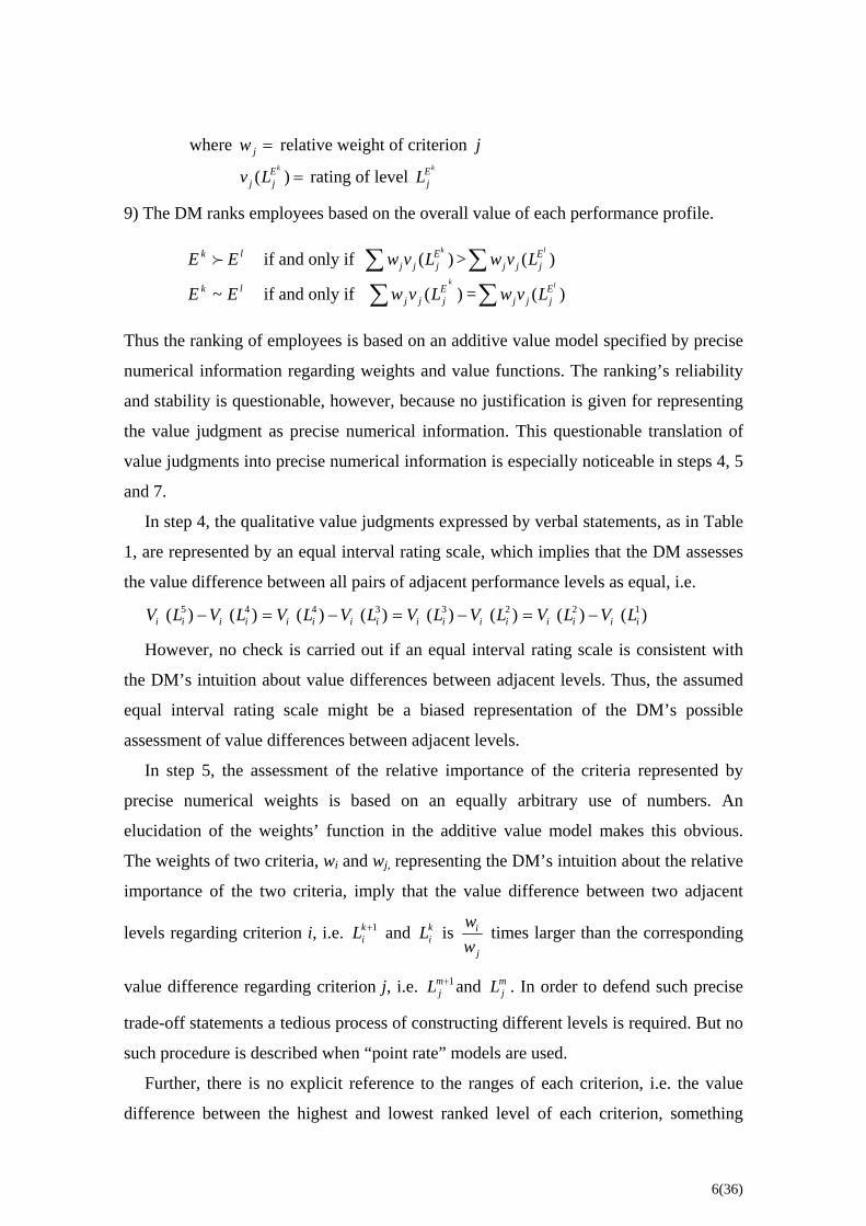
In step 4, the qualitative value judgments expressed by verbal statements, as in Table
1, are represented by an equal interval rating scale, which implies that the DM assesses
the value difference between all pairs of adjacent performance levels as equal, i.e.
)()()()()()()()( 12233445iiiiiiiiiiiiiiii LVLVLVLVLVLVLVLV −=−=−=−
However, no check is carried out if an equal interval rating scale is consistent with
the DM’s intuition about value differences between adjacent levels. Thus, the assumed
equal interval rating scale might be a biased representation of the DM’s possible
assessment of value differences between adjacent levels.
In step 5, the assessment of the relative importance of the criteria represented by
precise numerical weights is based on an equally arbitrary use of numbers. An
elucidation of the weights’ function in the additive value model makes this obvious.
The weights of two criteria, wi and wj, representing the DM’s intuition about the relative
importance of the two criteria, imply that the value difference between two adjacent
levels regarding criterion i, i.e. and is 1+kiL k
iLj
i
ww times larger than the corresponding
value difference regarding criterion j, i.e. and . In order to defend such precise
trade-off statements a tedious process of constructing different levels is required. But no
such procedure is described when “point rate” models are used.
1+mjL m
jL
Further, there is no explicit reference to the ranges of each criterion, i.e. the value
difference between the highest and lowest ranked level of each criterion, something
6(36)
which might give rise to biased and inappropriate assessments of the relative weights of
the criteria.
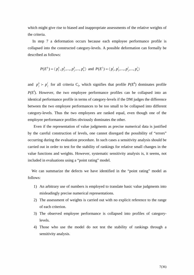
In step 7 a deformation occurs because each employee performance profile is
collapsed into the constructed category-levels. A possible deformation can formally be
described as follows:
⟩⟨= kn
kj
kkk ppppEP ,...,,...,.,)( 21 and ⟩⟨= ln
lj
lll ppppEP ,...,,...,.,)( 21
and for all criteria Clj
kj pp j, which signifies that profile P(Ek) dominates profile
P(El). However, the two employee performance profiles can be collapsed into an
identical performance profile in terms of category-levels if the DM judges the difference
between the two employee performances to be too small to be collapsed into different
category-levels. Thus the two employees are ranked equal, even though one of the
employee performance profiles obviously dominates the other.
Even if the representation of value judgments as precise numerical data is justified
by the careful construction of levels, one cannot disregard the possibility of “errors”
occurring during the evaluation procedure. In such cases a sensitivity analysis should be
carried out in order to test for the stability of rankings for relative small changes in the
value functions and weights. However, systematic sensitivity analysis is, it seems, not
included in evaluations using a “point rating” model.
We can summarize the defects we have identified in the “point rating” model as
follows:
1) An arbitrary use of numbers is employed to translate basic value judgments into
misleadingly precise numerical representations.
2) The assessment of weights is carried out with no explicit reference to the range
of each criterion.
3) The observed employee performance is collapsed into profiles of category-
levels.
4) Those who use the model do not test the stability of rankings through a
sensitivity analysis.
7(36)
Finally, we want to point out that this critique concerns common practice on the
evaluation of jobs and are not a general comment on the possibility of applying additive
value models in a well founded way. This is done, for instance, in Edwards and von
Winterfeld 1986, who demonstrate an evaluation procedure that gives rise to consistent
equal interval rating scales and appropriate weights.
In using the PRIME model, which supports imprecise value judgments, we avoid the
tedious task of constructing levels consistent with an equal interval rating scale and
assessing weights that can justify application of precise numerical information. (For
other attempts to model imprecise value judgments, see e.g. Spyridakos et al., 2001 and
Dasgupta, 1998.) In the next section we shall describe the PRIME model and its
application in the experiments concerning the evaluation of lecturer performance.
3. The PRIME model and evaluation of lecturer performance
3.1. PRIME model
The PRIME model is based on multi-attribute value theory. (For an extensive
description of the model and its applications, see Salo and Hämäläinen 2001.) The
PRIME model is implemented by a software package called PRIME Decisions, which is
a decision-aid that offers interactive decision support. PRIME Decisions can be
downloaded from: www.hut.fi\Units\SAL\Downloadables\ (Gustafsson et al, 2000).
In the PRIME model, the overall values of alternatives, which correspond to lecturers
in this study, are defined by an additive value model:
(1) )()( ∑= l
iil pvEV
The model can be rewritten as:
(2) , )()( ∑ ⋅= l
iNii
l pvwEV
where )()(
)()()( minmax
min
iiii
iiliil
iNi pvpv
pvpvpv−−
= , and by convention: =0, )( minii pv
which implies that: , and ]1,0[)( ∈l
iNi pv
)()( minmaxiiiii pvpvw −= ,
i.e. the attribute weights relate unit increases in normalized value functions to increases in the overall value.
8(36)
The overall value of an ideal profile, i.e. maxmax2
max1
max ,...,,)( npppEP = , is normalized to one, i.e.
(3) max max max max1
1 1( ) ,...., ( ) 1
n nN
n i i ii i
V E V p p w v p w= =
i= ⟨ ⟩ = ⋅ =∑ ∑ =
The PRIME Decisions has a feature called elicitation tour, which guides the DM
through a specific sequence of elicitation steps as follows:
Step 1: Ordinal value judgments
The DM is asked to rank performance regarding each criterion. The ranking is
represented by an ordinal value function:
(4) )( max
ii pv >>>> )(......)( kii
lii pvpv )( min
ii pv Step 2: Cardinal value judgments The DM is asked to elicit cardinal judgments regarding value differences between pairs
of ranked performances. The imprecise cardinal value judgments are represented as
interval-valued statements about ratio estimates regarding two value differences. For
instance, a comparison of value difference regarding pairs of adjacent performances can
be expressed as ratio estimates:
(5) 1
1
( ) ( )( ) ( )
l li i i i
k ki i i i
v p v pL Uv p v p
+
+
−≤ ≤
−
The interval [L, U] represents the degree of imprecision of cardinal value judgments
regarding the two value differences. However, the PRIME model supports ratio
estimates of value differences regarding arbitrary pairs of performances:
(6) n
( ) ( )( ) ( )
k li i i i
mi i i i
v p v pL Uv p v p
−≤ ≤
−, given that and ( ) (k l
i i i iv p v p> ) )( ) (m ni i i iv p v p>
Step 3: Weight assessment The DM is asked to assess the weights by:
9(36)
1) choosing a reference criterion, which is assigned the weight of 100%.
2) comparing the value difference between the highest and the lowest ranked
performance regarding each criterion relative to the corresponding value
difference of the reference criterion. The assessments are represented by
imprecise ratio estimates as:
(7) 100)()(
)()(100100100 minmax
minmax Upvpv
pvpvLUwwL
refrefrefref
iiii
ref
i ≤−−
≤⇔≤≤ ,
where [L, U] is the numerical interval mapping the degree of imprecision of weight
assessments.
The interval-valued statements expressed by the DM in an elicitation tour are
translated into a number of linear constraints, which define a set of feasible weights
as: 11
,......, { 0, 1}n
n w i ii
w w w S W w w w=
= ∈ ⊂ = ≥ ∑ = , and sets of feasible scores as:
[ ]( ) 0,1 , 1,...,l li i iv p S i n∈ ⊂ = , where = set of feasible scores for alternative , i.e.
lecturer , w. r. t. criterion i.
liS lE
lE
Based on the linear constraints the overall value of each performance profile is
represented by a value interval computed from the two linear programs:
(8) 1 1
( ) min ( ),max ( ) min ( ),max ( )n n
l l l li i i i i i
i iV E w v p w v p V E V E
= =
⎡ ⎤ l⎡ ⎤∈ =⎢ ⎥ ⎣ ⎦⎣ ⎦∑ ∑ ,
s.t. 1,......, nw w w S= ∈ w and [ ]( ) 0,1 , 1,...,l l
i i iv p S i n∈ ⊂ = .
10(36)
3.2. Dominance criteria and decision rules PRIME Decisions provides two dominance criteria and several decision rules to help the
DM rank the alternatives, in this case lecturer. The absolute dominance criterion is
defined as:
(9) min ( ) max ( )k l kDE E V E V E⇔ > l
i i i i <
According to the absolute dominance criterion lecturer Ek is ranked higher than El if the
smallest possible value of Ek exceeds the largest possible value of El. The absolute
dominance criterion can only be used for pairs of alternatives with nonoverlapping
value intervals. In the event of overlapping value intervals, the pairwise dominance
criterion has to be applied. The pairwise dominance criterion is defined as:
(10) , 1 1
max[ ( ) ( )] 0 max[ ( ) ( )] 0n n
k l l k l kD i i
i iE E V E V E w v p w v p
= =
⇔ − < ⇔ −∑ ∑ which holds for all combinations of feasible weights and feasible scores as:
1) 11
,..., { 0, 1}n
n w i ii
w w w S W w w w=
= ∈ ⊂ = ≥ ∑ = .
2) [ ]( ) 0,1 , 1,...,k ki i iv p S i n∈ ⊂ = and [ ]( ) 0,1 , 1,...,l l
i i iv p S i n∈ ⊂ = . According to this criterion lecturer Ek is ranked higher than lecturer El if and only if the
overall value of Ek exceeds that of El for all feasible solutions of the linear constraints
implied by the interval-valued statements in an elicitation tour. A non-dominance
relation occurs if the inequality in (10) does not hold, i.e. if there are overall values
implying that: . The interpretation of a non-dominance relation between
a lecturer E
( ) ( )lV E V E> k
k and a lecturer El is that the DM’s value information is not sufficiently
precise in order to determine a ranking between the two lecturers. In that case any of the
decision rules provided by PRIME Decisions can be applied.
In PRIME four decision rules are stated: 1) minimax 2) maximax 3) minimax regret
4) central values. The definition and the performance of the decision rules are discussed
in Salo and Hämläinen, 2001, who recommend on the basis of simulations the minimax
regret criterion and the application of central values since they consistently outperform
the other rules. In the experiments below we prefer to use the central values owing to
11(36)
ease of computations. The central values are defined as the mid-value of the value
intervals defined in (8).
In PRIME Decisions the computation of overall value intervals, weights, and
dominance structures is based on linear programs, the solution of which is based on
techniques that require plenty of calculation capacity, such as Simplex. PRIME
Decisions does not put any a priori restrictions on the number of criteria, the number of
alternatives, or the number of levels in a value tree. Computation time is roughly
proportional to the third power of the number of linear program problems. The number
of these problems, in turn, depends on the number of criteria, and alternatives
(Gustafson et al., 2001). With few criteria and alternatives the computation time is very
short. In the experiments below the computation time was about 30 seconds on a
Pentium III 833 MHz with 128 MB of RAM. After the calculation has finished the
results are available in a Windows menu.
3.3. Ranking of lecturers and salary compensation
Applying the dominance criteria allows a dominance structure over lecturers to be
established as regards an overall evaluation of their performance. The dominance
structure can serve as a guideline for salary setting as follows:
If a lecturer Ek is ranked higher than lecturer El according to the dominance
criteria then the DM can justify a higher salary compensation to lecturer Ek than
to lecturer El .
Thus despite imprecise value information the DM can justify different salary
compensation to different lecturers. However, if a non-dominance relation occurs
between two lecturers and it is the case that the DM cannot justify more precise value
information, then the DM cannot justify different salary compensation for the two
lecturers. However, the DM can decide to use the decision rules as recommended by
central values in PRIME Decisions in order determine a ranking between the two
lecturers.
There is also another reason that might force the DM to apply central values in order
to determine a ranking between lecturers related by non-dominance. The reason stems
from the fact that non-dominance is an intransitive relation. It might be the case, say,
12(36)
that non-dominance occurs between lecturer and , and between and ,
respectively, whereas dominates , i.e. denoting the non-dominance relation by
implies that: , and .
kE lE lE mEkE mE
" Non D−∼ " k lNon DE E−∼ l m
Non DE E−∼ k mDE E
Obviously, an intransitive order gives rise to inconsistent recommendations
concerning salary compensations; however, complementing the established partial
ranking with calculated central values solves the problem with intransitivity. However,
in the experiments presented in the next section, occurrences of non-dominance between
pairs of lecturers did not to give rise to intransitivity.
In this study the central values will also be used for another purpose. Since the
dominance criteria only determine a ranking, there is no information about relative
value differences among ranked lecturers. Central values can be used in order to
estimate reasonable value differences among lecturers, which can serve as a guideline
for setting appropriate relative salary compensation among lecturers. This is done in the
second experiment.
4. The experiments
4.1. Background
We have tested the usefulness of imprecise value judgments in the process of evaluating
employee performance by using them in two experiments, both carried out at Sweden’s
Södertörn College. Ever since its foundation in 1997, the University College has set its
lecturers’ salary according to a system of compensation based on individual
performance, assessed over specific periods of time. The “point rating” model discussed
above has frequently been used in evaluating Södertörn employee performance. This
enables us to use the defects of the “point rating” model, as identified above, as a point
of departure when evaluating the modeling of imprecise value judgments in the PRIME
model. The two experiments, which we have termed “Experiment I” and “Experiment
II”, are restricted, for methodological reasons, to a sample of six and seven lecturers
respectively. The lecturers are ranked solely on the basis of an assessment of their
relative scientific ability, which is defined by a number of sub-criteria.
4.2. Procedure
13(36)
The Södertörn experiment was preceded by a meeting at which two decision makers
taking part in experiment I and II, respectively, were alerted to the defects of the “point
rating” model and then introduced to the PRIME model. This was done by using a
simple example, in which four hypothetical employees were ranked according to two
well defined criteria. In our experience, an introduction of the PRIME model requires
careful elucidation by giving simple examples of the elicitation tasks to decision makers
lacking experience of multidimensional models supporting imprecise value judgments,
which differ in nature from simple point rating models as discussed in section 2. The
decision maker taking part in experiment I is a department chairman for a
multidisciplinary department and in experiment II is an associate professor and the
Department Chair of History at the University College.
The evaluation procedure carried out in the two experiments presented below was
based on personal interviews with the decision makers. Since the PRIME model
facilitates interactive work, the decision makers received immediate feedback on their
judgments. The evaluation procedure in both experiments took approximately two days,
excluding the time needed to sample employee performance data.
4.2.1. Experiment I
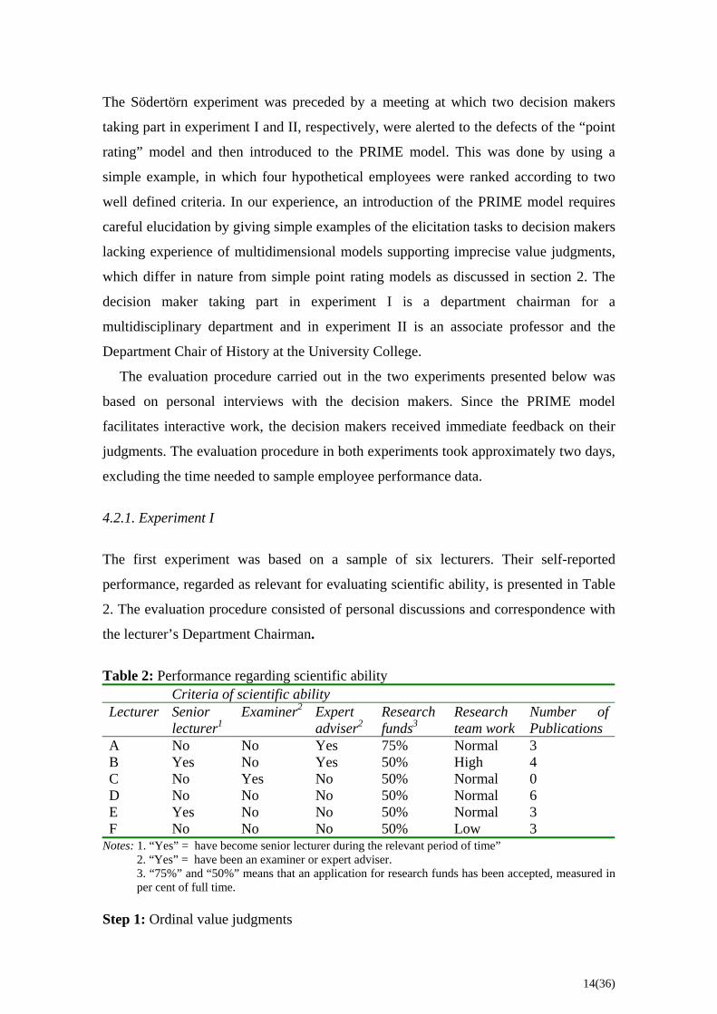
The first experiment was based on a sample of six lecturers. Their self-reported
performance, regarded as relevant for evaluating scientific ability, is presented in Table
2. The evaluation procedure consisted of personal discussions and correspondence with
the lecturer’s Department Chairman.
Table 2: Performance regarding scientific ability Criteria of scientific ability Lecturer Senior
lecturer1Examiner2 Expert
adviser2Research funds3
Research team work
Number of Publications
A No No Yes 75% Normal 3 B Yes No Yes 50% High 4 C No Yes No 50% Normal 0 D No No No 50% Normal 6 E Yes No No 50% Normal 3 F No No No 50% Low 3
Notes: 1. “Yes” = have become senior lecturer during the relevant period of time” 2. “Yes” = have been an examiner or expert adviser. 3. “75%” and “50%” means that an application for research funds has been accepted, measured in
per cent of full time. Step 1: Ordinal value judgments
14(36)
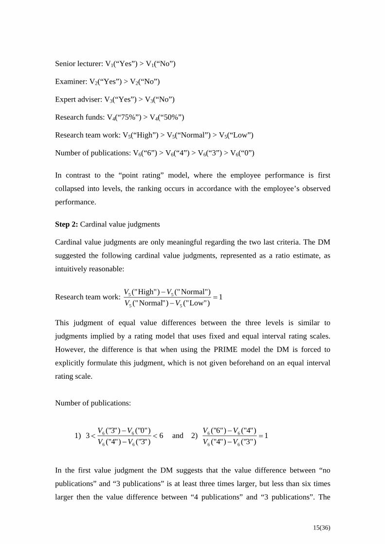
Senior lecturer: V1(“Yes”) > V1(“No”) Examiner: V2(“Yes”) > V2(“No”) Expert adviser: V3(“Yes”) > V3(“No”) Research funds: V4(“75%”) > V4(“50%”) Research team work: V5(“High”) > V5(“Normal”) > V5(“Low”) Number of publications: V6(“6”) > V6(“4”) > V6(“3”) > V6(“0”)
In contrast to the “point rating” model, where the employee performance is first
collapsed into levels, the ranking occurs in accordance with the employee’s observed
performance.
Step 2: Cardinal value judgments Cardinal value judgments are only meaningful regarding the two last criteria. The DM
suggested the following cardinal value judgments, represented as a ratio estimate, as
intuitively reasonable:
Research team work: 1)"Low(")"Normal(")Normal"(")High"("
55
55 =−
−VV
VV
This judgment of equal value differences between the three levels is similar to
judgments implied by a rating model that uses fixed and equal interval rating scales.
However, the difference is that when using the PRIME model the DM is forced to
explicitly formulate this judgment, which is not given beforehand on an equal interval
rating scale.
Number of publications:
1) 6)"3(")"4(")0"(")"3("
366
66 <−−
<VVVV
and 2) 1)3"(")"4(")"4(")6"("
66
66 =−−
VVVV
In the first value judgment the DM suggests that the value difference between “no
publications” and “3 publications” is at least three times larger, but less than six times
larger then the value difference between “4 publications” and “3 publications”. The
15(36)
imprecise value judgment represents the DM’s intuition concerning possible accuracy of
cardinal value judgments regarding publications. In other words, the DM thinks that
values outside the interval [3, 6] are intuitively unreasonable.
The second value judgment implies that the DM’s intuition suggests the value
difference between 3 and 4 publications is equal to the value difference between 4 and 6
publications. This corresponds to a decreasing marginal value regarding number of
publications. Thus the PRIME model can easily, in addition to imprecise value
judgments, consider decreasing (or increasing) marginal values.
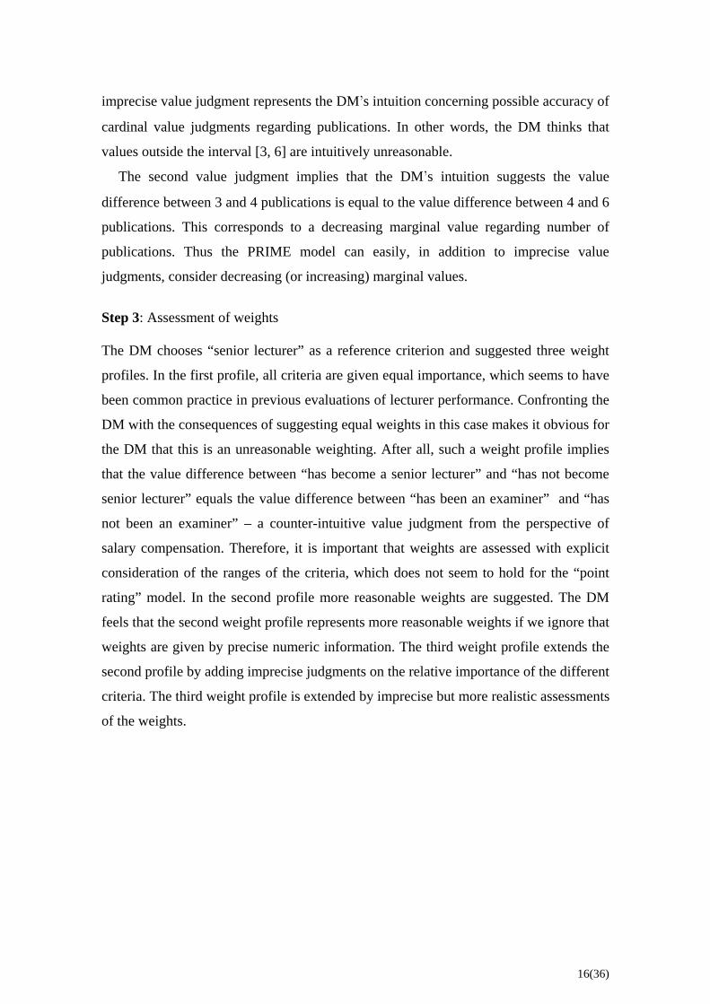
Step 3: Assessment of weights The DM chooses “senior lecturer” as a reference criterion and suggested three weight
profiles. In the first profile, all criteria are given equal importance, which seems to have
been common practice in previous evaluations of lecturer performance. Confronting the
DM with the consequences of suggesting equal weights in this case makes it obvious for
the DM that this is an unreasonable weighting. After all, such a weight profile implies
that the value difference between “has become a senior lecturer” and “has not become
senior lecturer” equals the value difference between “has been an examiner” and “has
not been an examiner” – a counter-intuitive value judgment from the perspective of
salary compensation. Therefore, it is important that weights are assessed with explicit
consideration of the ranges of the criteria, which does not seem to hold for the “point
rating” model. In the second profile more reasonable weights are suggested. The DM
feels that the second weight profile represents more reasonable weights if we ignore that
weights are given by precise numeric information. The third weight profile extends the
second profile by adding imprecise judgments on the relative importance of the different
criteria. The third weight profile is extended by imprecise but more realistic assessments
of the weights.
16(36)
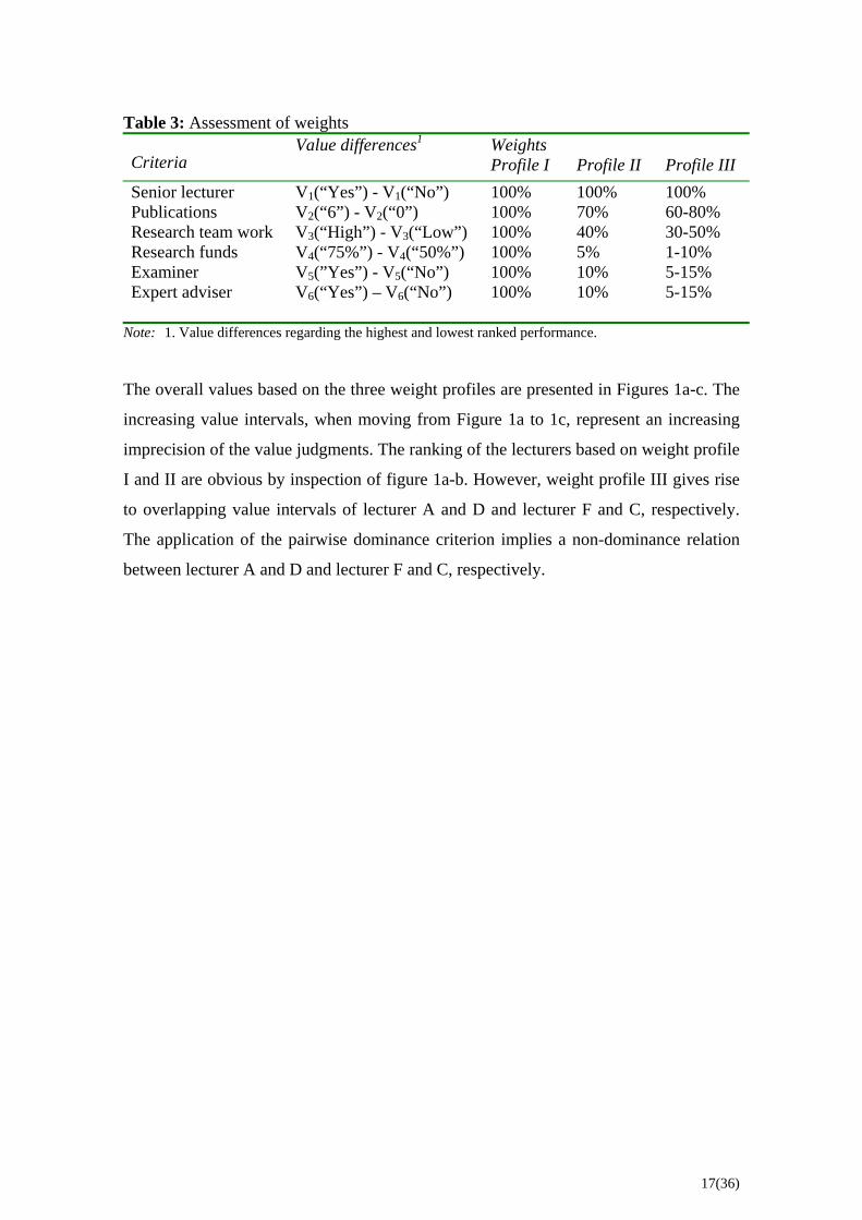
Table 3: Assessment of weights
Criteria Value differences1 Weights
Profile I Profile II
Profile III
Senior lecturer 100% 100% 100% Publications 100% 70% 60-80% Research team work 100% 40% 30-50% Research funds 100% 5% 1-10% Examiner 100% 10% 5-15% Expert adviser
V1(“Yes”) - V1(“No”) V2(“6”) - V2(“0”) V3(“High”) - V3(“Low”) V4(“75%”) - V4(“50%”) V5(”Yes”) - V5(“No”) V6(“Yes”) – V6(“No”) 100% 10% 5-15%
Note: 1. Value differences regarding the highest and lowest ranked performance.
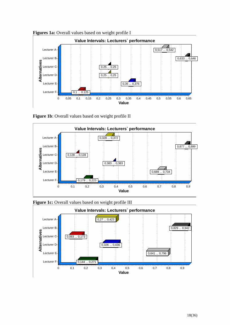
The overall values based on the three weight profiles are presented in Figures 1a-c. The
increasing value intervals, when moving from Figure 1a to 1c, represent an increasing
imprecision of the value judgments. The ranking of the lecturers based on weight profile
I and II are obvious by inspection of figure 1a-b. However, weight profile III gives rise
to overlapping value intervals of lecturer A and D and lecturer F and C, respectively.
The application of the pairwise dominance criterion implies a non-dominance relation
between lecturer A and D and lecturer F and C, respectively.
17(36)
Figures 1a: Overall values based on weight profile I
Value Intervals: Lecturers´ performance
Value0,650,60,550,50,450,40,350,30,250,20,150,10,050
Alte
rnat
ives
Lecturer F
Lecturer C
Lecturer D
Lecturer E
Lecturer A
Lecturer B
0,1 ... 0,125
0,25 ... 0,25
0,25 ... 0,25
0,35 ... 0,375
0,517 ... 0,542
0,633 ... 0,646
Figure 1b: Overall values based on weight profile II
Value Intervals: Lecturers´ performance
Value0,90,80,70,60,50,40,30,20,10
Alte
rnat
ives
Lecturer C
Lecturer F
Lecturer A
Lecturer D
Lecturer E
Lecturer B
0,128 ... 0,128
0,179 ... 0,223
0,328 ... 0,372
0,383 ... 0,383
0,689 ... 0,734
0,877 ... 0,899
Figure 1c: Overall values based on weight profile III
Value Intervals: Lecturers´ performance
Value0,90,80,70,60,50,40,30,20,10
Alte
rnat
ives
Lecturer C
Lecturer F
Lecturer A
Lecturer D
Lecturer E
Lecturer B
0,083 ... 0,173
0,144 ... 0,271
0,27 ... 0,423
0,326 ... 0,436
0,641 ... 0,796
0,829 ... 0,942
18(36)
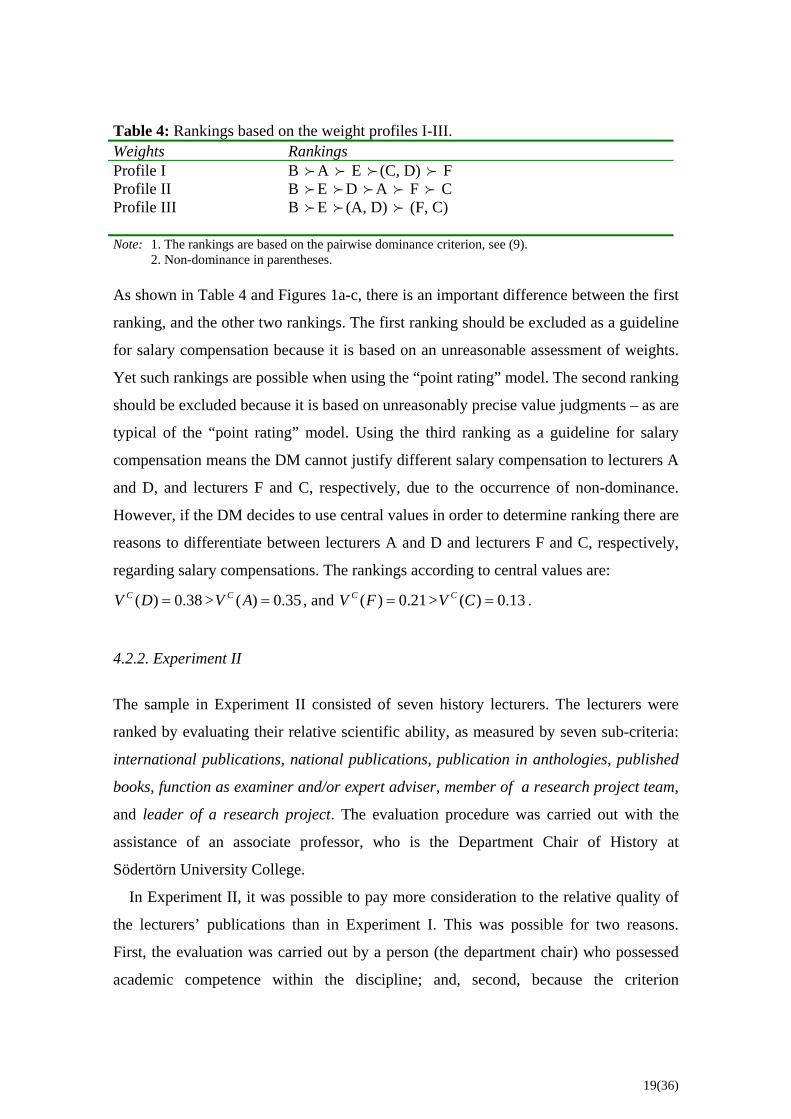
Table 4: Rankings based on the weight profiles I-III. Weights Rankings Profile I B A E (C, D) F Profile II B E D A F C Profile III B E (A, D) (F, C) Note: 1. The rankings are based on the pairwise dominance criterion, see (9). 2. Non-dominance in parentheses. As shown in Table 4 and Figures 1a-c, there is an important difference between the first
ranking, and the other two rankings. The first ranking should be excluded as a guideline
for salary compensation because it is based on an unreasonable assessment of weights.
Yet such rankings are possible when using the “point rating” model. The second ranking
should be excluded because it is based on unreasonably precise value judgments – as are
typical of the “point rating” model. Using the third ranking as a guideline for salary
compensation means the DM cannot justify different salary compensation to lecturers A
and D, and lecturers F and C, respectively, due to the occurrence of non-dominance.
However, if the DM decides to use central values in order to determine ranking there are
reasons to differentiate between lecturers A and D and lecturers F and C, respectively,
regarding salary compensations. The rankings according to central values are:
( ) 0.38CV D = > , and > . ( ) 0.3CV A = 5 3( ) 0.21CV F = ( ) 0.1CV C =
4.2.2. Experiment II
The sample in Experiment II consisted of seven history lecturers. The lecturers were
ranked by evaluating their relative scientific ability, as measured by seven sub-criteria:
international publications, national publications, publication in anthologies, published
books, function as examiner and/or expert adviser, member of a research project team,
and leader of a research project. The evaluation procedure was carried out with the
assistance of an associate professor, who is the Department Chair of History at
Södertörn University College.
In Experiment II, it was possible to pay more consideration to the relative quality of
the lecturers’ publications than in Experiment I. This was possible for two reasons.
First, the evaluation was carried out by a person (the department chair) who possessed
academic competence within the discipline; and, second, because the criterion
19(36)
”Production of publications” was divided into four sub-criteria: international
publications, national publications, publication in anthologies, and published books.
In the presentation of the evaluation procedure the lecturers are denoted by the letters
A to G. The evaluation of performance is expressed as =)(BVI value of lecturer B’s
performance regarding criterion I, etc.
The evaluation procedure as defined by the PRIME model occurs in the three steps.
In this case, step 2 (the cardinal value judgments) is divided into two parts: (a) precise
cardinal value judgments, and (b) imprecise cardinal value judgments. The evaluation
process in steps 2a and 2b is based on intuitive reasoning using hypothetical changes in
the observed performance profiles of the seven lecturers. The reason for asking the DM
to give precise but tentative cardinal value judgments is based on our assumption that
such an approach makes it easier for the DM to understand the meaning of cardinal
value judgments, bearing in mind that the DM is unfamiliar with multi-attribute value
models such as PRIME. In order to explain the intuitive reasoning which underlies
precise and imprecise cardinal value judgments, a more detailed description is provided
for the evaluation of the first criterion: international publications.
The evaluation procedure is carried out as follows:
Criterion I: “International publications” Table 5: Performance regarding international publications Lecturer Performance B “2 publications” G “2 working papers” F “2 conference papers” A, C, D, E “No publications” Step 1: Ordinal value judgments Table 5 presents the DM’s ordinal value judgments regarding “international
publications”, which are represented by a value function:
V1(“2 publications”) = 1 > V1(“2 working papers”) > V1(“2 conference papers”) >
V1(“No publications”) = 0.
20(36)
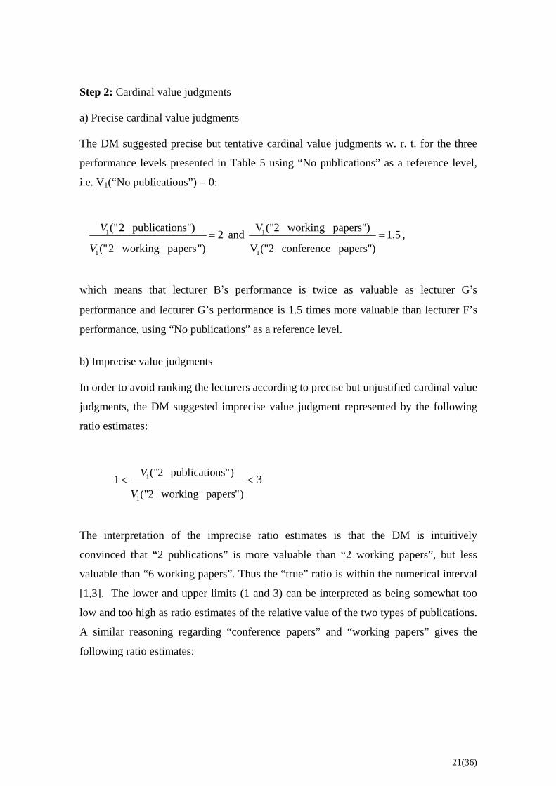
Step 2: Cardinal value judgments a) Precise cardinal value judgments The DM suggested precise but tentative cardinal value judgments w. r. t. for the three
performance levels presented in Table 5 using “No publications” as a reference level,
i.e. V1(“No publications”) = 0:
1
1
("2 publications") 2("2 working papers")
V
V= and 1
1
V ("2 working papers") 1.5V ("2 conference papers")
= ,
which means that lecturer B’s performance is twice as valuable as lecturer G’s
performance and lecturer G’s performance is 1.5 times more valuable than lecturer F’s
performance, using “No publications” as a reference level.
b) Imprecise value judgments In order to avoid ranking the lecturers according to precise but unjustified cardinal value
judgments, the DM suggested imprecise value judgment represented by the following
ratio estimates:
3)"papersworking2("
)ns"publicatio2("11
1 <<V
V
The interpretation of the imprecise ratio estimates is that the DM is intuitively
convinced that “2 publications” is more valuable than “2 working papers”, but less
valuable than “6 working papers”. Thus the “true” ratio is within the numerical interval
[1,3]. The lower and upper limits (1 and 3) can be interpreted as being somewhat too
low and too high as ratio estimates of the relative value of the two types of publications.
A similar reasoning regarding “conference papers” and “working papers” gives the
following ratio estimates:
21(36)
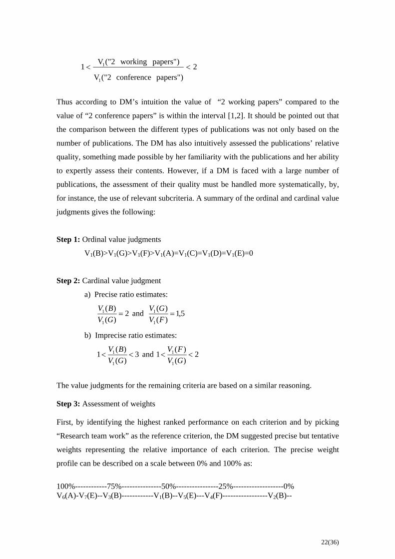
2)papers"conference("2V
)papers"working("2V11
1 <<
Thus according to DM’s intuition the value of “2 working papers” compared to the
value of “2 conference papers” is within the interval [1,2]. It should be pointed out that
the comparison between the different types of publications was not only based on the
number of publications. The DM has also intuitively assessed the publications’ relative
quality, something made possible by her familiarity with the publications and her ability
to expertly assess their contents. However, if a DM is faced with a large number of
publications, the assessment of their quality must be handled more systematically, by,
for instance, the use of relevant subcriteria. A summary of the ordinal and cardinal value
judgments gives the following:
Step 1: Ordinal value judgments
V1(B)>V1(G)>V1(F)>V1(A)=V1(C)=V1(D)=V1(E)=0
Step 2: Cardinal value judgment
a) Precise ratio estimates:
2)()(
1
1 =GVBV and 5,1
)()(
1
1 =FVGV
b) Imprecise ratio estimates:
3)()(1
1
1 <<GVBV and 2
)()(1
1
1 <<GVFV
The value judgments for the remaining criteria are based on a similar reasoning.
Step 3: Assessment of weights First, by identifying the highest ranked performance on each criterion and by picking
“Research team work” as the reference criterion, the DM suggested precise but tentative
weights representing the relative importance of each criterion. The precise weight
profile can be described on a scale between 0% and 100% as:
100%------------75%---------------50%----------------25%-------------------0% V6(A)-V7(E)--V3(B)------------V1(B)--V5(E)---V4(F)-----------------V2(B)--
22(36)
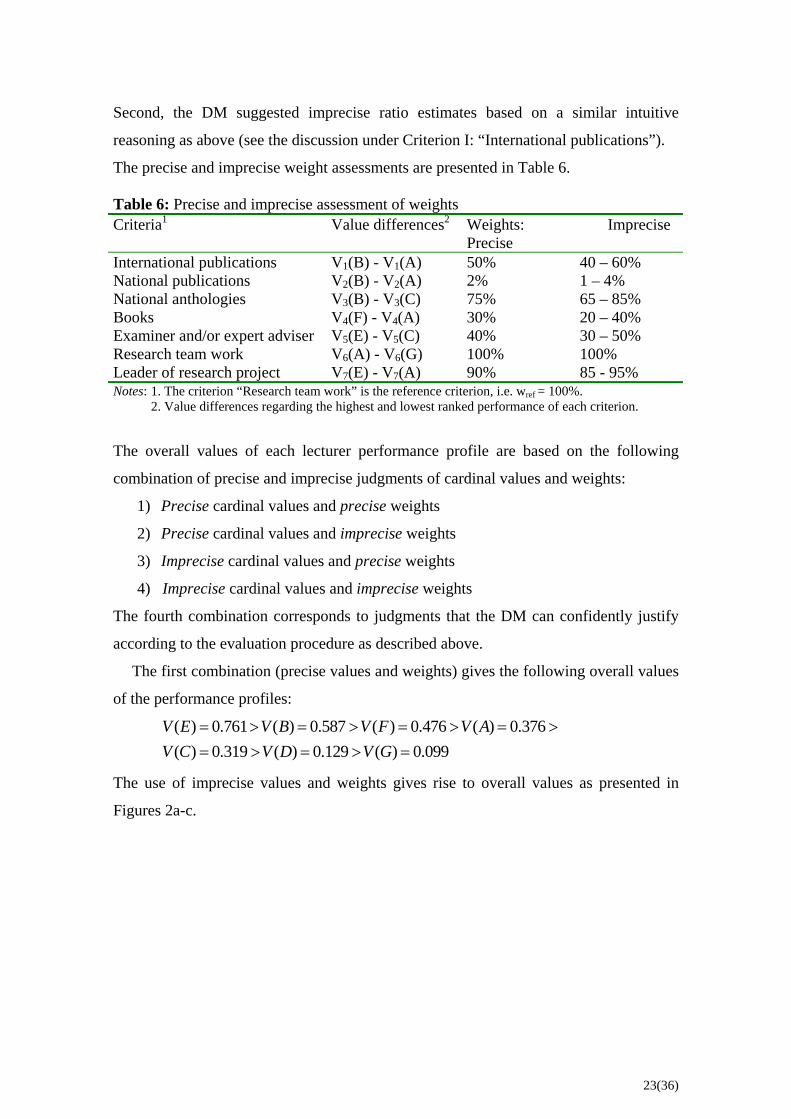
Second, the DM suggested imprecise ratio estimates based on a similar intuitive
reasoning as above (see the discussion under Criterion I: “International publications”).
The precise and imprecise weight assessments are presented in Table 6. Table 6: Precise and imprecise assessment of weights Criteria1 Value differences2 Weights:
Precise Imprecise
International publications V1(B) - V1(A) 50% 40 – 60% National publications V2(B) - V2(A) 2% 1 – 4% National anthologies V3(B) - V3(C) 75% 65 – 85% Books V4(F) - V4(A) 30% 20 – 40% Examiner and/or expert adviser V5(E) - V5(C) 40% 30 – 50% Research team work V6(A) - V6(G) 100% 100% Leader of research project V7(E) - V7(A) 90% 85 - 95% Notes: 1. The criterion “Research team work” is the reference criterion, i.e. wref = 100%. 2. Value differences regarding the highest and lowest ranked performance of each criterion.
The overall values of each lecturer performance profile are based on the following
combination of precise and imprecise judgments of cardinal values and weights:
1) Precise cardinal values and precise weights
2) Precise cardinal values and imprecise weights
3) Imprecise cardinal values and precise weights
4) Imprecise cardinal values and imprecise weights
The fourth combination corresponds to judgments that the DM can confidently justify
according to the evaluation procedure as described above.
The first combination (precise values and weights) gives the following overall values
of the performance profiles:
( ) 0.761 ( ) 0.587 ( ) 0.476 ( ) 0.376( ) 0.319 ( ) 0.129 ( ) 0.099
V E V B V F V AV C V D V G
= > = > = > = >= > = > =
The use of imprecise values and weights gives rise to overall values as presented in
Figures 2a-c.
23(36)
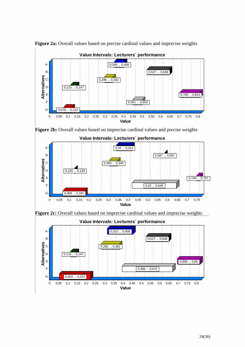
Figure 2a: Overall values based on precise cardinal values and imprecise weights
Value Intervals: Lecturers´ performance
Value0,80,750,70,650,60,550,50,450,40,350,30,250,20,150,10,050
Alte
rnat
ives
G
D
C
A
F
B
E
0,076 ... 0,122
0,115 ... 0,147
0,296 ... 0,342
0,349 ... 0,406
0,451 ... 0,503
0,527 ... 0,648
0,705 ... 0,813
Figure 2b: Overall values based on imprecise cardinal values and precise weights
Value Intervals: Lecturers´ performance
Value0,750,70,650,60,550,50,450,40,350,30,250,20,150,10,050
Alte
rnat
ives
G
D
C
A
F
B
E
0,069 ... 0,181
0,129 ... 0,129
0,304 ... 0,349
0,34 ... 0,421
0,42 ... 0,646
0,587 ... 0,587
0,749 ... 0,767
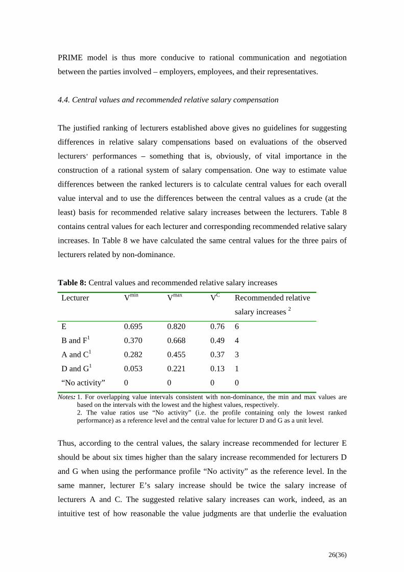
Figure 2c: Overall values based on imprecise cardinal values and imprecise weights
Value Intervals: Lecturers´ performance
Value0,80,750,70,650,60,550,50,450,40,350,30,250,20,150,10,050
Alte
rnat
ives
G
D
C
A
F
B
E
0,053 ... 0,223
0,115 ... 0,147
0,282 ... 0,381
0,315 ... 0,456
0,396 ... 0,672
0,527 ... 0,648
0,695 ... 0,82
24(36)
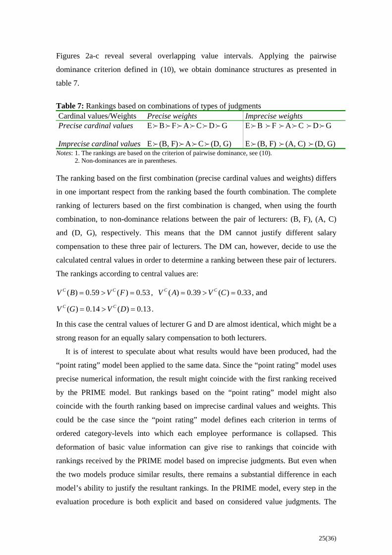
Figures 2a-c reveal several overlapping value intervals. Applying the pairwise
dominance criterion defined in (10), we obtain dominance structures as presented in
table 7.
Table 7: Rankings based on combinations of types of judgments Cardinal values/Weights Precise weights Imprecise weights Precise cardinal values E B F A C D G E B F A C D G Imprecise cardinal values E (B, F) A C (D, G) E (B, F) (A, C) (D, G)
Notes: 1. The rankings are based on the criterion of pairwise dominance, see (10). 2. Non-dominances are in parentheses. The ranking based on the first combination (precise cardinal values and weights) differs
in one important respect from the ranking based the fourth combination. The complete
ranking of lecturers based on the first combination is changed, when using the fourth
combination, to non-dominance relations between the pair of lecturers: (B, F), (A, C)
and (D, G), respectively. This means that the DM cannot justify different salary
compensation to these three pair of lecturers. The DM can, however, decide to use the
calculated central values in order to determine a ranking between these pair of lecturers.
The rankings according to central values are:
( ) 0.59 ( ) 0.53C CV B V F= > = , , and
.
( ) 0.39 ( ) 0.33C CV A V C= > =
( ) 0.14 ( ) 0.13C CV G V D= > =
In this case the central values of lecturer G and D are almost identical, which might be a
strong reason for an equally salary compensation to both lecturers.
It is of interest to speculate about what results would have been produced, had the
“point rating” model been applied to the same data. Since the “point rating” model uses
precise numerical information, the result might coincide with the first ranking received
by the PRIME model. But rankings based on the “point rating” model might also
coincide with the fourth ranking based on imprecise cardinal values and weights. This
could be the case since the “point rating” model defines each criterion in terms of
ordered category-levels into which each employee performance is collapsed. This
deformation of basic value information can give rise to rankings that coincide with
rankings received by the PRIME model based on imprecise judgments. But even when
the two models produce similar results, there remains a substantial difference in each
model’s ability to justify the resultant rankings. In the PRIME model, every step in the
evaluation procedure is both explicit and based on considered value judgments. The
25(36)
PRIME model is thus more conducive to rational communication and negotiation
between the parties involved – employers, employees, and their representatives.
4.4. Central values and recommended relative salary compensation
The justified ranking of lecturers established above gives no guidelines for suggesting
differences in relative salary compensations based on evaluations of the observed
lecturers’ performances – something that is, obviously, of vital importance in the
construction of a rational system of salary compensation. One way to estimate value
differences between the ranked lecturers is to calculate central values for each overall
value interval and to use the differences between the central values as a crude (at the
least) basis for recommended relative salary increases between the lecturers. Table 8
contains central values for each lecturer and corresponding recommended relative salary
increases. In Table 8 we have calculated the same central values for the three pairs of
lecturers related by non-dominance.
Table 8: Central values and recommended relative salary increases
Lecturer Vmin Vmax VC Recommended relative
salary increases 2
E 0.695 0.820 0.76 6
B and F1 0.370 0.668 0.49 4
A and C1 0.282 0.455 0.37 3
D and G1 0.053 0.221 0.13 1
“No activity” 0 0 0 0
Notes: 1. For overlapping value intervals consistent with non-dominance, the min and max values are based on the intervals with the lowest and the highest values, respectively.
2. The value ratios use “No activity” (i.e. the profile containing only the lowest ranked performance) as a reference level and the central value for lecturer D and G as a unit level.
Thus, according to the central values, the salary increase recommended for lecturer E
should be about six times higher than the salary increase recommended for lecturers D
and G when using the performance profile “No activity” as the reference level. In the
same manner, lecturer E’s salary increase should be twice the salary increase of
lecturers A and C. The suggested relative salary increases can work, indeed, as an
intuitive test of how reasonable the value judgments are that underlie the evaluation
26(36)
procedure. If several of the proposed relative salary increases appear obviously counter-
intuitive, then an adjustment of some of the basic value judgments is called for. An
iterative process switching between basic value judgments and intuitive judgments
about resulting salary compensation might end with a reflective equilibrium concerning
a rational basis for salary compensation. Due to the restricted number of criteria used in
the evaluation of employee performance in the experiment such a test would seem
unfruitful and is beyond the scope of the present study.
4.5. The decision maker’s perception of the PRIME-model
We end the section by reporting about the DMs’ perception of the PRIME-model as
compared to models as the “point rating” model presented in the second section. After
the evaluation processes were finished we encouraged the DMs to attend a meeting to
discuss their perception of the two approaches. The DM who took part in the second
experiment was the only one to attend the meeting. As department chair of history at
Södertörn University College she is directly responsible for the evaluation of lecturer
performance and for recommending salaries. The evaluation of lecturer performance
takes place every year. The DM has an extensive experience of evaluating the
performance of history lecturers.
When evaluating lecturer performance, the DM has used simplistic models, such as
point rating models, and intuitive considerations. As we will stress the DM is
completely unfamiliar with structured multi-attribute value models, such as PRIME. For
this reason we believe that the qualitative information based on the interviews despite
its anecdotal quality gives important insight about a DM’s perception of strengths and
weaknesses of theoretically well-founded multi-attribute value models such as PRIME.
Such information is of course important for the implementation of more full-scale
experiments in this type of evaluation context.
The interview with the DM was structured as follows. Firstly, we asked specific
questions about her perception of the elicitation tasks such as ordinal and imprecise
cardinal value judgements. Secondly, we asked questions about her perception of the
assessment of weights as defined in PRIME. Thirdly, we asked her to comment on the
weaknesses and strengths of the PRIME-model as regards its usefulness and ease of
understanding. (For extensive studies of comparisons of multi-attribute value models
from a DM’s point view, see Wallenius 1975, Belton 1986, Buchanan 1994).
27(36)
Comments on evaluation tasks as ordinal and imprecise cardinal value judgments
The first step in an elicitation tour to rank-order lecturers w. r. t. using each criterion
was, according to the DM, a rather easy task. Further, the DM regarded this very basic
step in multi-attribute evaluations as very instructive since it became obvious to the DM
that value differences between various observed performance levels are not at all
consistent with an equally spaced interval scale based on semantic categories as
presented in Table 1. It seems that the DM was aware of the fact that such a scale
imposes unjustified restrictions on her value judgements. The DM gave two obvious
reasons for continuing to use fixed scales such as 1 to 5 in order to represent evaluation
of lecturer performance. Firstly, the DM was not familiar with approaches based on
multi-attribute models, such as PRIME, while “point rating” models are promoted by
executives at the university college and are widely used when jobs and employee
performance are evaluated. Belton and Stewart (2002 pp. 320-237) report on the use of
similar simplistic and theoretically unfounded models in other application areas.
Secondly, the DM deemed it as necessary to use simplistic models such as point rating
models when the number of lecturers or criteria became too large. In such cases the DM
judged that it is not recommended to rely solely on a purely intuitive evaluation of
lecturer performance.
The second step in an elicitation tour to elicit imprecise cardinal value judgements
represented by numerical intervals was regarded by the DM as more demanding than
rank-ordering observed performance. However, after a detailed instruction on how to
interpret the numerical intervals the DM perceived that expressing cardinal value
judgements in an imprecise manner represented by numerical intervals to be a more
reliable representation of her intuitive value judgements compared to the restrictive
representations in point rating models. Further, according to the DM being able to
express imprecise cardinal value judgements increased her awareness of the defects of
using a fixed scale in this type of evaluation context, where, as the DM pointed out,
most of the criteria are qualitative in nature. However, the DM pointed to the obvious
problem of how to justify precise upper and lower limits of the numerical interval
representing the imprecise value judgements. Salo and Hämäläinen (2003) discuss the
interpretation of precise upper and lower limits.
Comments on the assessment of weights
28(36)
The DM perceived the assessment of weights to be the most demanding process in an
elicitation tour. She gave two reasons for this judgment. Firstly, the assessment of
weights as defined in PRIME was unfamiliar to the DM, as is expected. The DM was
not able state a definition of the weights other than to say in loose terms that a weight
assigned to a criterion is a function of its importance for the achievement of main
objectives for the university college, which seems to imply that the DM assumed that
the weights are independent of how the measurement scales for value judgments are
constructed in the specific evaluation model. The DM found it very difficult to
understand the definition of weights in the PRIME-model. Detailed instructions, based
on simple examples, were required in order to make the DM realize the function of
weights in a multi-attribute value model. The unambiguous interpretation of weights
among DMs in situations that are multi-attribute fashioned is well-documented (see
Belton and Stewart 2002, pp. 288-291, Weber 1993, Weber and Borcherding 1993).
Secondly, the DM stressed that, even if weights as defined in PRIME are used the
task is difficult, since the assessment of weights means that an evaluative comparison
takes place between different types of performance as compared to intra-criterion
evaluations. The DM perceived that her intuition about reasonable cardinal value
judgements across various criteria was less stable compared to intra-criterion
evaluations.
However, one important advantage of the PRIME approach to encouraging tradeoffs
between explicitly stated differences between performances and across various criteria
is, according to the DM, that it increased her awareness that intuition about reasonable
tradeoffs has to be guided by the purpose of evaluation. And in this case the purpose of
the evaluation concerns giving reasons for relative salary compensation based on
various observed performance.
Considering the DM’s perception of the assessment of weights, we conclude that this
elicitation task plays a key role in successfully implementing multi-attribute value
models, such as PRIME. This means that when introducing the PRIME-model to DMs
unfamiliar with multi-attribute value models, specific care should be taken when the
definition of weights is explained. It is also important to stress that in order to make
meaningful trade-off statements the DM has to be aware of the meaning of the overall
value. In this evaluation situation the overall values are used to give reasons for relative
salary compensation. Mustajoki et al (2005) discuss practical and procedural matters
concerning weighting methods.
29(36)
Comments on weaknesses and strengths of the PRIME-model
Besides the DM’s perception of details in an elicitation tour we also asked questions
about her perception of other weaknesses with the PRIME-model. Firstly, as to be
expected the DM finds the PRIME-model more involved than a “point rating” model,
which means that a DM is dependent on an analysis and that an evaluation process
becomes time consuming. The DM perceived that the PRIME-model, at least as in its
current design, will not be a realistic approach for evaluation of lecturer performance in
larger departments at the university college. The department involved in Experiment II
contained eleven lecturers, which the DM perceived as an obvious realistic number for
an implementation of multi-attribute value models such as PRIME, even when the
number of criteria considered in Experiment II increased. Secondly, the synthesis of
value judgements and decision criteria used to determine final ranking of lecturers with
respect to an overall evaluation have a design that is too technical to be understood by
DMs unfamiliar with multi-attribute value models. This means that an application of
PRIME gives rise to a “black box” effect on its users. Thirdly, this “black box” effect,
as the DM stressed, may be the most important weakness with more sophisticated multi-
attribute models such as PRIME, since it will give rise to difficulties in communicating
the results to lecturers. Thus, due to this “black-box” effect, results of the evaluation and
suggested salary compensation might receive a low confidence among lecturers.
In contrast to this serious weakness the DM finds that a structured multi-attribute
value approach as defined in PRIME increased her discipline and awareness in the
evaluation process, which means, among other things, that it increased her awareness of
problems concerning the proper definitions of criteria, the elicitation of reasonable value
judgments and how to evaluate the final results.
We summarize the DM’s perception of the PRIME-model in terms of weaknesses
and strengths. Its weaknesses are: 1) The evaluation process is time-consuming, which
means that the application of PRIME seems to be restricted to evaluations of a relative
small number of lecturers. 2) The DM has to be supported by a decision analyst. 3) Due
to a “black-box” effect the results might be difficult to communicate to lecturers.
Its strengths are: 1) The possibility of expressing intuitive but imprecise cardinal
value judgement means that clustering of different performances into the same
categories is avoided. 2) The explicit way of defining weights related to relative
differences between highest and lowest performance. 3) The structured way of carrying
30(36)
out the evaluation process increases the discipline and the awareness of problems
concerning the proper definitions of criteria, the elicitation of value judgments and how
to evaluate the final results.
5. Conclusions
This paper began by pointing out a number of defects inherent to using “point rating”
models for evaluating employee performance. The two experiments show how the
PRIME model’s ability to synthesize imprecise value judgments corrects many of these
defects:
1) Ordinal and cardinal value judgments are applied to observed employee
performance, thus avoiding the deformation occurring when employee
performance is collapsed into category-levels.
2) The assessment of weights is explicitly based on relative value differences
regarding the highest and lowest ranked performance of each criterion, thus
avoiding severe biased assessment of weights.
3) Imprecise judgments of cardinal values and weights are represented by
numerical intervals, thus avoiding deformation of imprecise value judgment into
unrealistic precise numerical statements.
4) The evaluation process occurs along well-defined steps forcing the decision
maker to explicitly express his or her value judgments and increasing the
discipline of the decision maker in the evaluation process.
By interviewing the DM we also identified two important issues that should be
investigated in a follow-up study. Firstly, due the technical design of the PRIME-model
the DM finds it difficult to understand the logic of the model, and believed that it will be
difficult to communicate the results of an evaluation. Therefore, a comparison of the
PRIME-model and simplistic models such as point rate models as regards effectiveness
in terms of communication of results should carried out. Secondly, the assessment of
weights is, according to the DM, the most demanding elicitation task for both formal
and substantial reasons. This means that in order to improve the applicability and the
reliability of the PRIME-model in this type of evaluation context, the functioning of
various procedures used for assessing weights should be investigated.
31(36)

The study concludes by indicating two paths for further investigation as suggested by
the two experiments and the interview. The first would be a follow-up study that
included a greater number of employees and a greater range of criteria (such as
pedagogical skills). Second, a follow-up study examining the possibility of defining the
performance profiles by a value tree structure. The evaluation of a value tree, which is
supported by the PRIME model, makes it possible to carry out more detailed
evaluations of complex criteria, which should be partitioned into a number of sub-
criteria. One such complex and important criterion is “Quality of publications”, of
which a more detailed assessment would be possible using this method.
32(36)
References Arnault EJ, Gordon L, Joines DH, Phillips MG. 2001. An experimental study of job
evaluation and comparable worth. Industrial and Labor Relations Review 54: 806-815.
Belton V. A. 1986. Comparison of the analytic hierarchy process and a simple multi-attribute value function. European Journal of Operational Research 26: 7-21.
Belton V, Stewart TJ. 2002. Multiple Criteria Decision Analysis – An Intergrated Approach. Kluwer Academic Publishers: Boston, Dordrecht and London.
Buchanan JT. 1994. An experimental evaluation of interactive MCDM methods and the decision making process. Journal of the Operational Research Society. 45: 1050-1059.
Dasgupta S, Chakraborty M. 1998. Job evaluation in fuzzy environment. Fuzzy Sets and Systems 100: 71-76.
Garcia-Diaz A, Hoog GL. 1983. A mathematical Programming Approach to Salary Administration. Computational and Industrial Engineering 7: 7-13.
Gustafsson J, Salo A, Gustafsson T. 2001. PRIME Decisions: An interactive Tool for Value Tree Analysis. In Multiple Criteria Decision Making in The New Millennium, Köksalan M, Zionts S (eds.). Lecture Notes in Economics and Mathematical Systems 507. Springer-Verlag: Berlin: 165-186
Gustafsson J, Gustafsson T, Salo A. 2000. PRIME Decisions – An Interactive Tool for Value Tree Analysis. V. 1.0, Computer software, System Analysis Laboratory, Helsinki University of Technology. (www.sal.hut.fi/Downloadables).
Harriman A, Holm C. 2001. Steps to Pay Equity – An easy and quick method for the evaluation of work demands. URL:http://www.equalpay.nu/docs/en/steps_to_pay_equity.pdf (2004-01-13).
Keeney RL, Raiffa H. 1976. Decision with Multiple Objectives: Preferences and Value Tradeoffs. John Wiley: New York.
Kira M. 2000. Work Organization, Compensation and Payment Systems – An exploratory report for SALTSA/Work Organization-subprogram. Royal Institute for Technology, Industrial Work Science, Institute for Industrial Economics and Management, Stockholm, Sweden.
Lazear EP. 1998. Personnel Economics. The MIT Press: Cambridge, Massachusetts, London, England.
Salo A, Hämäläinen RP. 2001. Preference Ratios in Multiattribute Evaluation (PRIME) – Elicitation and Decision Procedures Under Incomplete Information. IEEE Transactions on System, Man and Cybernetics – Part A: Systems and Humans 31: 533-545.
Salo A, Hämäläinen RP. 1992. Preference Assessment by Imprecise Ratio Statements. Operation Research 40: 1053-1061
Salo A, Hämäläinen RP. 2003. Preference Programming, Manuscript submitted for publication, Systems Analysis Laborartory, Helsinki University of Technology, Finland
Mustajoki J, Hämäläinen RP, Salo A. 2005. Decision Support by Interval SMART/SWING - Incorporating Imprecision in the SMART and SWING Methods, Decision Sciences, 36: 317-339.
Spyridakos A, Siskos Y, Yannacopoulas D. and Skouris A. 1999. Multicriteria job evaluation for large organizations. European Journal of Operational Research 130: 375-387.
33(36)

Troutt MD,Tadisina SK. 1992. The Analytic Hierarchy Process as a Model Base for Merit Salary Recommendation System. Mathematical Computational Modeling 16: 99-105.
von Winterfeldt E, Edwards W. 1986. Decision Analysis and Behavioral Research. Cambridge University Press: New York.
Weber M. 1993. The Effect of Attribute Ranges on Weights in Multiattribute Utility Measurements. Management Science 39: 937-943.
Weber M, Borcherding K. 1993. Behavioral influences on weigt judgments in multiattribute decision making. European Journal of Operational Reserch 67: 1-12.
Wallenius J. 1975. Comparative Evaluation of Some Interactive Approaches to Multicriteria Optimization. Management Science 21: 1387-1396
34(36)
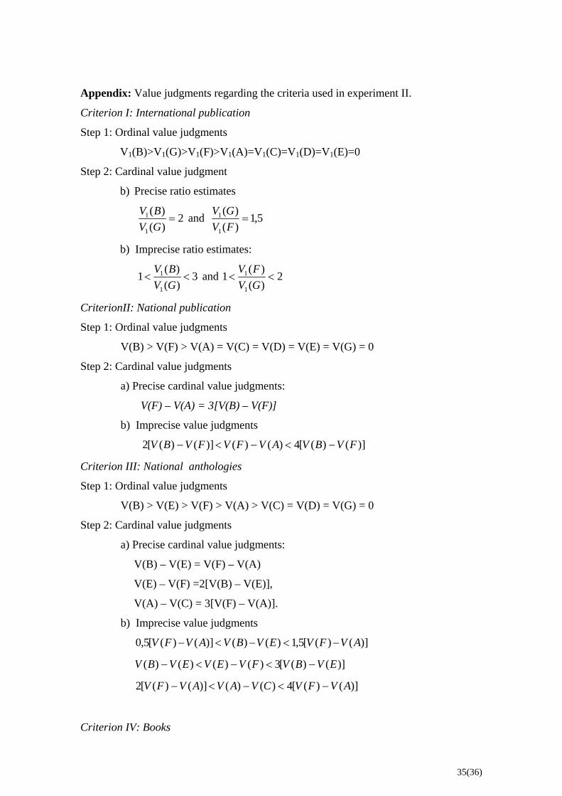
Appendix: Value judgments regarding the criteria used in experiment II.
Criterion I: International publication
Step 1: Ordinal value judgments
V1(B)>V1(G)>V1(F)>V1(A)=V1(C)=V1(D)=V1(E)=0
Step 2: Cardinal value judgment
b) Precise ratio estimates
2)()(
1
1 =GVBV and 5,1
)()(
1
1 =FVGV
b) Imprecise ratio estimates:
3)()(1
1
1 <<GVBV and 2
)()(1
1
1 <<GVFV
CriterionII: National publication
Step 1: Ordinal value judgments
V(B) > V(F) > V(A) = V(C) = V(D) = V(E) = V(G) = 0
Step 2: Cardinal value judgments
a) Precise cardinal value judgments:
V(F) – V(A) = 3[V(B) – V(F)]
b) Imprecise value judgments
)]()([4)()()]()([2 FVBVAVFVFVBV −<−<−
Criterion III: National anthologies
Step 1: Ordinal value judgments
V(B) > V(E) > V(F) > V(A) > V(C) = V(D) = V(G) = 0
Step 2: Cardinal value judgments
a) Precise cardinal value judgments:
V(B) – V(E) = V(F) – V(A)
V(E) – V(F) =2[V(B) – V(E)],
V(A) – V(C) = 3[V(F) – V(A)].
b) Imprecise value judgments
)]()([5,1)()()]()([5,0 AVFVEVBVAVFV −<−<−
)]()([3)()()()( EVBVFVEVEVBV −<−<−
)]()([4)()()]()([2 AVFVCVAVAVFV −<−<−
Criterion IV: Books
35(36)
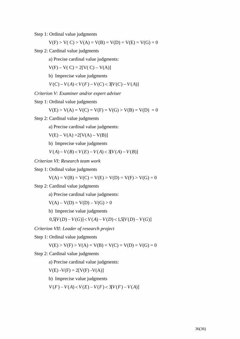
Step 1: Ordinal value judgments
V(F) > V( C) > V(A) = V(B) = V(D) = V(E) = V(G) = 0
Step 2: Cardinal value judgments
a) Precise cardinal value judgments:
V(F) – V( C) = 2[V( C) – V(A)]
b) Imprecise value judgments
)]()([3)()()()( AVCVCVFVAVCV −<−<−
Criterion V: Examiner and/or expert adviser
Step 1: Ordinal value judgments
V(E) > V(A) = V(C) = V(F) = V(G) > V(B) = V(D) = 0
Step 2: Cardinal value judgments
a) Precise cardinal value judgments:
V(E) – V(A) =2[V(A) – V(B)]
b) Imprecise value judgments
)]()([3)()()()( BVAVAVEVBVAV −<−<−
Criterion VI: Research team work
Step 1: Ordinal value judgments
V(A) = V(B) = V(C) = V(E) > V(D) = V(F) > V(G) = 0
Step 2: Cardinal value judgments
a) Precise cardinal value judgments:
V(A) – V(D) = V(D) – V(G) > 0
b) Imprecise value judgments
)]()([5,1)()()]()([5,0 GVDVDVAVGVDV −<−<−
Criterion VII: Leader of research project
Step 1: Ordinal value judgments
V(E) > V(F) > V(A) = V(B) = V(C) = V(D) = V(G) = 0
Step 2: Cardinal value judgments
a) Precise cardinal value judgments:
V(E) -V(F) = 2[V(F) -V(A)]
b) Imprecise value judgments
)]()([3)()()()( AVFVFVEVAVFV −<−<−
36(36)