Embed Size (px)
Citation preview
I
UNIVERSITY OF SHEFFIELD DEPARTMENT OF COMPUTER SCIENCE
UNDERGRADUATE DISSERTATION
An Evaluation of
Birdsong Recognition Techniques
Author: Supervisor:
Scott Shaw Dr. Phil Green
This report is submitted in partial fulfilment of the requirement for the degree of Bachelor of
Science with Honours in Computer Science by Scott Shaw
4th May 2011

II
Signed Declaration
All sentences or passages quoted in this report from other people's work have been
specifically acknowledged by clear cross-referencing to author, work and page(s). Any
illustrations which are not the work of the author of this report have been used with the
explicit permission of the originator and are specifically acknowledged. I understand that
failure to do this amounts to plagiarism and will be considered grounds for failure in this
project and the degree examination as a whole.
Name: Scott Shaw
Signature:
Date: 4th
May 2011
III
Abstract
The use of several different methods of automated speech recognition is investigated to
determine the techniques that produce the overall highest accuracy result. The methods
GMM, HMM, ANN, SVM and a hybrid tandem ANN/HMM classifiers are investigated. The
final results are then compared to the commercial product Song Scope, which is used as a
benchmark for the results produced. All recognition is attempted on whole recording due to
this method mostly reflecting how a classifier would be used in a real world situation. The
highest accuracy was obtained from the Tandem ANN/HMM followed by the HMM, ANN
and the GMM classifiers.
IV
Contents
1. Introduction ..................................................................................................... 1
1.1 Background .................................................................................................. 1
1.2 Commercial Concepts .................................................................................. 3
1.2.1 Conservation and Entertainment ....................................................... 3
1.2.2 Other Animals .................................................................................... 3
1.2.3 Commercial Growth .......................................................................... 3
1.3 Bird Vocalisation in Relation to Human Speech ......................................... 4
1.4 Detection Complications .............................................................................. 5
1.5 Digital Pattern Processing ............................................................................ 7
2. Classification Techniques ............................................................................... 8
2.1 Artificial Neural Network (ANN)................................................................ 8
2.2 Support Vector Machine (SVM) .................................................................. 8
2.3 Gaussian Mixture Model (GMM) ................................................................ 9
2.4 Hidden Markov Model (HMM) ................................................................. 11
2.6 Hybrid Systems .......................................................................................... 12
3. Previous Research ......................................................................................... 13
3.1 McIlraith et al (1995) ................................................................................. 14
3.2 Cia et al (2010) ........................................................................................... 14
3.3 Ross (2006) ................................................................................................ 17
3.4 Fagerlund (1997) ........................................................................................ 18
3.5 Arogant (Song Scope) (2009) .................................................................... 19
3.6 Departmental Work .................................................................................... 20
3.6.1 Brown et al (2009) ........................................................................... 20
3.6.2 Gelling (2010) .................................................................................. 21
3.6.2.1 Experiments and Results .................................................... 23
3.7 Literature Discussion ................................................................................. 24
4. Summary ........................................................................................................ 25
5. Pattern Recognition Implementation .......................................................... 26
V
5.1 Data and Bird Species ................................................................................ 27
5.2 Signal Processing and Syllable Extraction ................................................ 28
6. Classification .................................................................................................. 30
6.1 Implementation and Toolkits ..................................................................... 30
6.2 Classifiers ................................................................................................... 30
6.2.1 Gaussian Mixture Model ................................................................. 30
6.2.2 Hidden Markov Model .................................................................... 31
6.2.3Artificial Neural Network ................................................................ 31
6.2.4 Support Vector Machine .................................................................. 32
6.2.5 Tandem System ............................................................................... 32
7. Post processing .............................................................................................. 33
7.1 Frame-by-Frame Voting ............................................................................ 33
7.2 Viterbi Algorithm ....................................................................................... 33
7.3 Confusion Matrix ....................................................................................... 34
8. Experiments ................................................................................................... 34
9. Results ............................................................................................................ 36
9.1 Gaussian Mixture Model Results ............................................................... 36
9.1.1 Results ............................................................................................. 36
9.1.2 Evaluation ....................................................................................... 37
9.2 Hidden Markov Model Results .................................................................. 38
9.1.1 Results ............................................................................................. 40
9.1.2 Evaluation ....................................................................................... 40
9.3 Support Vector Machine Results ............................................................... 41
9.3.1 Results ............................................................................................. 41
9.3.2 Evaluation ....................................................................................... 42
9.4Artificial Neural Network Results .............................................................. 43
9.4.1 Varying the Number of Features .................................................... 43
9.4.1.1 Results ............................................................................... 43
9.4.2 Varying the Number of Hidden Neurons ....................................... 44
9.4.2.1 Results ............................................................................... 44
9.4.3 Evaluation ....................................................................................... 45
9.4Tandem ANN/HMM system Results .......................................................... 46
9.5.1 Varying the Number of Cepstral Coefficients ................................ 46
9.5.1.1 Results ............................................................................... 47
VI
9.5.2 Varying the Number of Hidden Neurons ....................................... 47
9.5.2.1 Results ............................................................................... 48
9.5.3 Varying the Mixtures and States .................................................... 48
9.5.2.1 Results ............................................................................... 48
9.5.5 Evaluation ....................................................................................... 50
9.6 Song Scope ................................................................................................ 51
9.5.2.1 Results .......................................................................................... 51
10. Overall Results Review .............................................................................. 52
10.1 Median Confusion Matrix ........................................................................ 53
11. Objectives ..................................................................................................... 55
12. Issues............................................................................................................. 56
13. Discussion ..................................................................................................... 57
14. Conclusion .................................................................................................... 58
15. Future Directions ........................................................................................ 59
16. Bibliography ................................................................................................ 60
VII
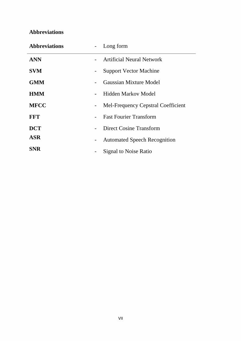
Abbreviations
Abbreviations - Long form
ANN - Artificial Neural Network
SVM - Support Vector Machine
GMM - Gaussian Mixture Model
HMM - Hidden Markov Model
MFCC - Mel-Frequency Cepstral Coefficient
FFT - Fast Fourier Transform
DCT - Direct Cosine Transform
ASR
- Automated Speech Recognition
SNR
- Signal to Noise Ratio
1
1. Introduction
1.1 Background
A large number of biological studies obtain recordings of the vocalisation of birds which are
gather in the field for technical research [7] and in addition to this, many amateurs and
enthusiasts undertake similar activities as a hobby. Many of these recording are analysed
using representation of the bird songs in spectrogram form, which are used to identify birds
or species from their calls. The research is used to monitor the ecosystem with regards to the
avian population. Generally, research of this kind is conducted in natural environments,
which leads to technical difficulties with regards to locating and monitoring these birds.
Many of these difficulties can be overcome by using audio detection equipment to produce
audio files of the vocalisations and are later analysed by experts. Once the data has been
analysed it can be used to determine specific information about ecosystem as well as other
information, for instance the species diversity in a given area. The use of bird vocalisation is
an important way to conduct environment monitoring, ecological censuring and biodiversity
assessment [10].
Current techniques for obtaining this data involve a device being placed in situ within
a test area, which is near to the species or habitat that is to be monitored. Alternatively, an
individual or a group will attend and conduct a census by human observation. Both methods
are currently widely used, but also have their limitations and draw backs. For instance, if a
recording is to be taken, the device has to be taken to, and retrieved from the site, which is a
time consuming process. An expert then has to listen to, and segment the data, either
manually or automatically, and subsequently makes an observation which is also extremely
time consuming. Alternatively, if the birds are monitored on location, some birds may be less
inclined to vocalise if there are humans present [1]. Both methods require trained experts who
are able to identify the birds; the techniques are long and arduous processes, involving many
hours dedicated to the listening and deciphering of the vocalisations by experts who are
skilled in identifying the different species. Conducting these inspections manually can be
prone to errors since cross checking is required which duplicates the work and effort, [7].
Additionally, experts are usually expensive to employ and training. All of which inevitably
leads to increased cost. There is, therefore, a need for an automated system that can produce
objective and reproducible results, with greater speed, reduced cost and greater accuracy,
when compared to the procedures that are currently available to carry out this analysis.
Previous work carried out to create a solution has centred on current techniques for
automated speech recognition (ASR) which is used in human research. With bird vocalisation
this is seen as a typical pattern processing problem with a signal pre-processing feature
extraction and classification section [5]. The problem of recognition is comparable to that of
human speech recognition with bird vocalisation being relatively simplistic compared to
human speech. The use of automated recognition is able to facilitate recognition of birds as
well. Human vocalisations consist of subunits organised into hierarchical phones, words and
sentences, and this also applies to birds, with their elements, syllables and phrases [7]. So far,
comparatively little work has been done in fulfilling development of software that is able to
2
apply this sort of recognition to animal vocalisations. Most of the work that has been carried
out in this field has focused on the use of clean recordings that have been produced in a
controlled environment with little focus on providing a tool that is able to automatically
detect birds songs in a real-world environment. [8].
It is therefore necessary for research to be carried out to identify and create a
technology that is able to incorporate known techniques for automated human speech
recognition into a working model for birds that is capable of encapsulating real-time data and
processing in a way that will allow true representation of the bird population in a given area.
There is a spectrum of ideas and approaches that have been applied to the research of
automated speech recognition (ASR) and many of these approaches have been used in an
attempt to solve bird song recognition. However, much of this research has focused on the
possibilities of the technique being used for bird recognition rather than actually applying it
to the problem. Much of this research has focused around the use of Gaussian Mixture
Models (GMM) and Hidden Markov Models (HMM) classifiers, with a commercial
application called Songscope that is currently available which uses a HMM classifier. Other
research has focused on the use of; Dynamic Time Warping (DTW), Artificial Neural
Networks (ANN), Support Vector Machines (SVM) and other methods currently used in
ASR which have been relatively unsuccessful. This research highlights how difficult it is to
determine which method is the most reliable; there is no standardised data set being used, the
quality of the recording sample can be variable and this makes it difficult to make effective
comparisons.
Other work conducted in The University of Sheffield Department of Computer
Science by Brown et al [4] and Gelling [1] have begun to try and develop this research in to a
standardised project. Brown et al initially undertook the research using DTW, GMM and
SVM models and compared their results to the commercial application SongScope [2] using a
database of material that was obtained from the internet. Gelling [1]. Then carried on this
research and investigated the significance of temporal information in recognition using GMM
and HMM models. He constructed the HMM model and pre-processing algorithms in
accordance with those defined by SongScope [2]. This work was undertaken using the data
set obtained by Brown et al, it was concluded that the data set was too small to give clear
indication of the relative success and it was highlighted that any future work should be
carried out on a larger dataset to determine the relative effectiveness of produced results. This
was due to a high variation of results obtained [1]
Before this research was conducted more data was sourced to fulfil the
recommendation by Gelling [1. Due to this the work conducted by Gelling will be repeated
applying the HMM and GMM classifiers that was constructed and applying the techniques to
the new data. As well as this, the commercial product SongScope [2] will be used as a
benchmark to compare the effectiveness of the models produced. Once this has been done,
the main focus of this dissertation will be to attempt to produce an Artificial Neural Networks
(ANN) and Support Vector Machine (SVM) classifiers to compare results on the data. Also,
further investigation will be made into other viable options. This should give a clear
indication of the possible uses for these classifier models and their comparative accuracy to
that of SongScope and the work conducted by Gelling [1] on a larger dataset.
3
In the following sections the complications that arise from attempting bird song
recognition is explored and methods that have been used to overcome these, also, the possible
commercial application of any software that is produced. Next, is a comparison between the
formation of birdsongs and human speech followed by the problems of pattern processing
with regards to computers, after this a look at other methods that have been used to undertake
similar projects with an evaluation of other literature in relation to the work that will be
conducted within this paper, finally, an overview of the results gained from the experiments
conducted and a conclusion is drawn from these results.
1.2 Commercial Concepts
In this section is a brief overview what a developed system could be used for and commercial
implications.
1.2.1 Conservation and Entertainment
Although not always conceived, birds are an integral part of the ecosystem. They serve many
purposes that include distribution of seeds, rodent and insect control and food source for birds
of prey. Being able to monitor populations, allows experts to help maintain a bio diverse
environment. There is therefore a demand for a product that is able to undertake bird
recognition work efficiently and provide a successful way to monitor species.
As well as experts there are many groups and individuals who are passionately
interested in tracking and identifying avian populations and software could aid these
enthusiasts in their quest for understanding and enjoyment.
1.2.2 Other Animals
Although this paper specifically looks at creating an application that could be used solely for
birds, there is also the possibility of a applying the algorithm to other animals, including bats,
underwater creatures, frogs and other animals that produce sounds. Such an application could
be used widely in the natural world to conduct automated conservation work within a given
area and to determine the ecological diversity and environmental monitoring. This could
enable greater understanding of animal‟s behaviour and help conservation efforts with
regards to protecting precious habitats for endangers species.
1.2.3 Commercial growth
Although birds are present in our cities they are affected, like other animals, by the ever
expanding human population which is causing loss of habitation and other essential
requirements vital for animals survival. As humans become increasingly aware of the
destruction they are causing due to building of factories, business parks and expanding cities
into areas that once were natural environments the ecosystem is closely managed to protect
animals against extinction. Several methods of managing the adverse effects have been used
4
by governments and controlling bodies. Many of these projects study the damage that such
developments have on the local ecosystems which enables areas of natural importance to be
preserved. There is evidentially a market for a product that is able to carry out this process
automatically [8].
1.3 Bird Vocalisation in Relation to Human Speech
Birds produce sounds for various reasons, with the majority falling in the categories of songs
and calls [5]. Songs are generally longer than calls and are more musical, harmonic and are
generally sung to attract mates or define territory. Calls are generally shorter, not learnt and
are used to alter other birds of impending dangers including predators. However, not all birds
are songbirds with only around 50% being able to produce songs. The remainder are able to
produce just calls that enable them to communicate with others. [5] Songbirds are able to
produce complex sounds due to them being able to control the production of sound better
which enables them to have a larger repertoire. [5]
Both birds and humans produce sound of a complex acoustic signal nature [9]. This is
done by moving air through the vocal system whilst expiration, it is this which produces the
sound. This process is fairly well understood in humans. Air from expiration creates a wave-
form upon the vocal folds. The components of the waveform are modified by the remainder
of the vocal tract. This includes the nose, mouth, lips and teeth [9]. This procedure is believed
to be very similar to the way bird produce sound with air passing through an organ called the
syrinx, which is situated between the trachea and bronchi. The beak and tongue are believed
to aid the forming of the vocalisations. Although there are differences with regards to
structure, both animals are able to produce a highly structured and high speed changing
vocalisation which requires an elaborate neural control and coordination of the vocal system
[9].
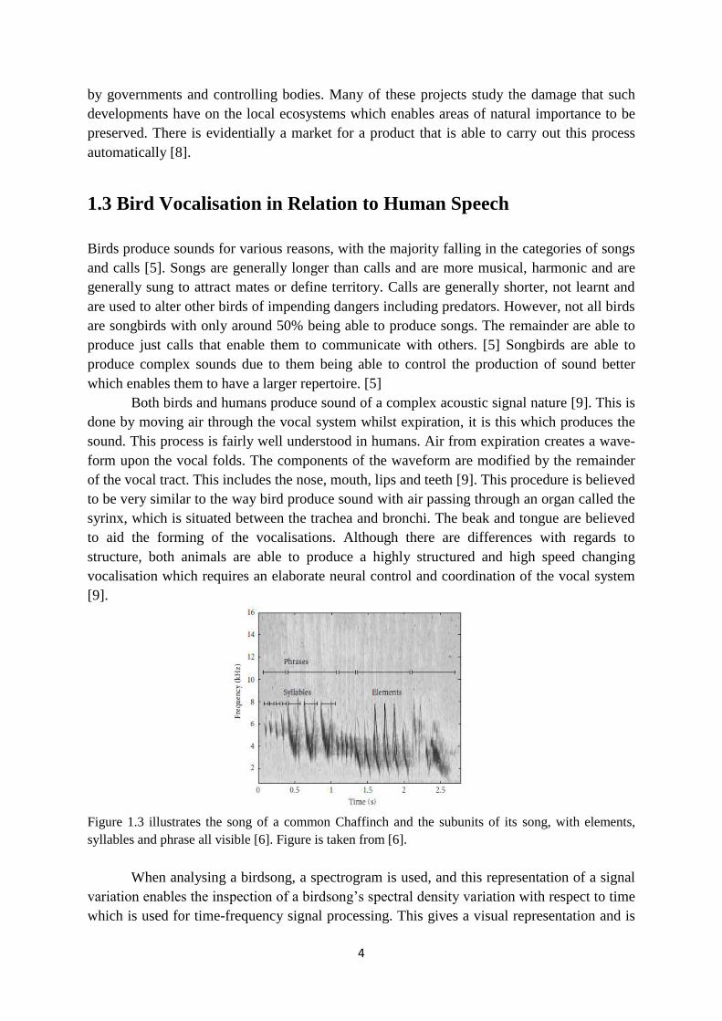
Figure 1.3 illustrates the song of a common Chaffinch and the subunits of its song, with elements,
syllables and phrase all visible [6]. Figure is taken from [6].
When analysing a birdsong, a spectrogram is used, and this representation of a signal
variation enables the inspection of a birdsong‟s spectral density variation with respect to time
which is used for time-frequency signal processing. This gives a visual representation and is

5
the method used to identify birdsongs. The most basic level of a song is represented by an
element; these are the smallest continuous sections that are locatable on a spectrogram. These
elements are comparable to the phonetic unit or basic unit of speech. The elements are
generally contained within a group that are called syllables, which are separated by an
interval of silence. Interesting, if a bird is startled by a bright light or sound it will not stop
producing a sound until it has finished the syllable that it is currently producing [9]. This is a
good indication that the syllable is the basic processing unit of a birdsong, as posited for
speech [9].
Syllables are structured into phrases, which can be either a string of similar or
different syllables. The majority of birds are able to produce phrases in a set order, whereas
some species like the warbler and the mockingbird are able to form sequences of phrases in
fixed or variable order. The formation of these phrase and syllables are generally never
random and fit set rules on timing and sequencing depending on the given species. This
ordering of phrases is similar to the formation of sentences using words implying the use of
grammar to form birdsong literature. The grammatical structure of a birdsong is called the
song syntax.
Birds like humans, learn the ability to produce songs from their parents. This learning
procedure enables the young to begin producing structured sounds, but at the same time
limits the individual to a set repertoire of the species to which they belong and the subset of
sounds that are produced. Additionally, the set ordering of these elements are also learnt. The
formation of sounds enables the structuring of a species and the ordering of elements into
syllables and songs, similar to the formation of sounds into words and sentences as in
humans. This formation of songs enables standardisation within a species. Although,
variations within species exist through dialects and individual specific songs, the use of song
formation, similar to sentences with a set number of sounds, enables recognition in the same
way as in humans. This should therefore conclude that research using the temporal
characteristics of a bird song should be beneficial to species recognition.
Since there is a smaller subset of sounds available for a bird to produce, this makes
bird songs relatively simple in comparison to human speech. It is therefore conceivable that
the use of human automated speech recognition algorithms as used in speech analysis, is
adaptable to be used in birdsong recognition. It is however, important to take into
consideration the syntax of how syllables are combined, as well as the spectral and feature
vectors when analysing [2]. Nevertheless, there are issues and limiting factors with regards to
vocalisation acquisition compared to human speech. The limitations which need to be
overcome are reviewed in the next section.
1.4 Detection Complications
The use of bioacoustics monitoring is a functional tool for evaluation of the bird population.
[8]. There are however, extenuating circumstances that have to be taken into consideration
with regards to using automated speech recognition technology when applying it to birdsong
recognition. The collection of data samples from humans, for example, is far easier than that
of collecting from birds. This is due to the fact that the researcher is able to collect data in a
6
controlled environment, tell the speaker when and what to say which allows them to obtain
recording with little to no periods of extended silence and produce a sample that has a high
signal-to-noise (SNR) ratio.
Compare this to the collection of bird vocalisations in a real- world situation where
samples have to be collected in the bird‟s natural environment, which maybe an unrestricted
distance away from the recording device. Additionally, there are obstacles like trees and
foliage that may interfere by causing echo and reverberations on the audio files. Further
complications arise due to the large amount of background noise affecting the recording, with
noise associated with other animals, other birds, human presence including planes, trains and
natural occurring events like wind and rain. This leads to material that has a low SNR and the
recognisor may have difficulty recognising the bird‟s species. Additional signal processing
requirements are therefore needed before the raw audio file can be used, such as putting the
signal through bandpass filters and normalization
Another issue is that human speech has a particular bandwidth that is concentrated in
an approximate 4 kHz bandwidth which is unique to humans. However, with birds, sounds
can vary significantly with different species being able to produce sounds in different
bandwidths. These may occur in a large frequency range anywhere from 10Hz to 10,000Hz
[5]. The variation of the vocalisation makes detection difficult, with some calls being short
and having a narrowband with distinctive spectral features. Whilst other songs, maybe be
long with complex spectral differences. Due to this variation it becomes difficult to produce
an algorithm that is able to successfully detect such a broad spectral frequency.
Also, the vast amount of training data that is available for human speech recognition
makes it easier to model individual variations due to the collated data of thousands of
individuals. Much of the research carried out on bird vocalisation is limited to a much smaller
amount of test data, which makes it difficult to be able to model the large variations in many
species [2].
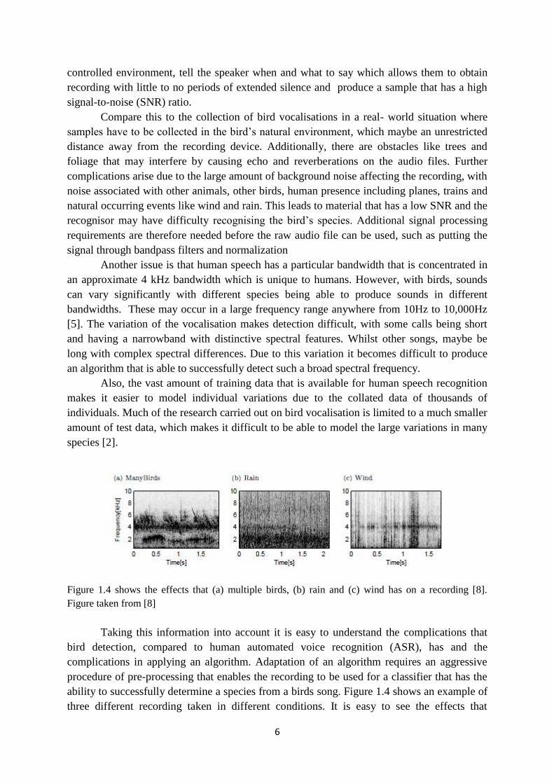
Figure 1.4 shows the effects that (a) multiple birds, (b) rain and (c) wind has on a recording [8].
Figure taken from [8]
Taking this information into account it is easy to understand the complications that
bird detection, compared to human automated voice recognition (ASR), has and the
complications in applying an algorithm. Adaptation of an algorithm requires an aggressive
procedure of pre-processing that enables the recording to be used for a classifier that has the
ability to successfully determine a species from a birds song. Figure 1.4 shows an example of
three different recording taken in different conditions. It is easy to see the effects that
7
background noise has on the recordings and the need to remove the majority of this noise
before the song can be successfully recognised, without successful removal of this
interference a lower than expected accuracy is achieved.
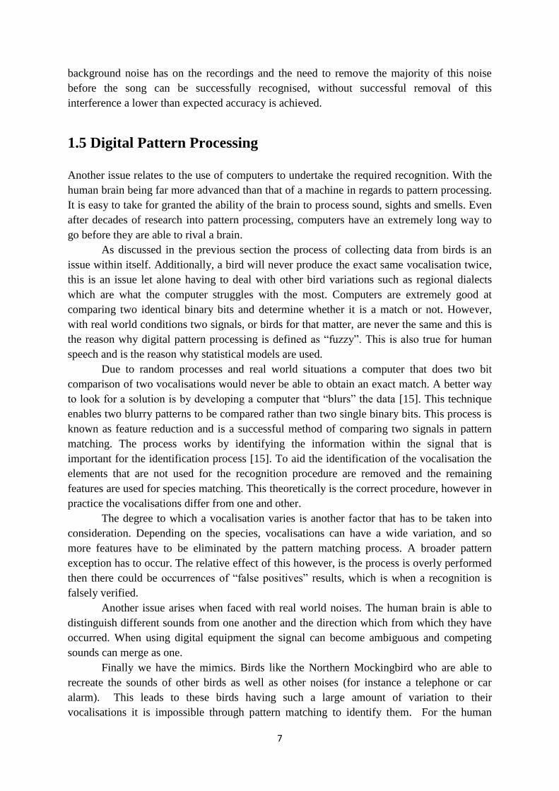
1.5 Digital Pattern Processing
Another issue relates to the use of computers to undertake the required recognition. With the
human brain being far more advanced than that of a machine in regards to pattern processing.
It is easy to take for granted the ability of the brain to process sound, sights and smells. Even
after decades of research into pattern processing, computers have an extremely long way to
go before they are able to rival a brain.
As discussed in the previous section the process of collecting data from birds is an
issue within itself. Additionally, a bird will never produce the exact same vocalisation twice,
this is an issue let alone having to deal with other bird variations such as regional dialects
which are what the computer struggles with the most. Computers are extremely good at
comparing two identical binary bits and determine whether it is a match or not. However,
with real world conditions two signals, or birds for that matter, are never the same and this is
the reason why digital pattern processing is defined as “fuzzy”. This is also true for human
speech and is the reason why statistical models are used.
Due to random processes and real world situations a computer that does two bit
comparison of two vocalisations would never be able to obtain an exact match. A better way
to look for a solution is by developing a computer that “blurs” the data [15]. This technique
enables two blurry patterns to be compared rather than two single binary bits. This process is
known as feature reduction and is a successful method of comparing two signals in pattern
matching. The process works by identifying the information within the signal that is
important for the identification process [15]. To aid the identification of the vocalisation the
elements that are not used for the recognition procedure are removed and the remaining
features are used for species matching. This theoretically is the correct procedure, however in
practice the vocalisations differ from one and other.
The degree to which a vocalisation varies is another factor that has to be taken into
consideration. Depending on the species, vocalisations can have a wide variation, and so
more features have to be eliminated by the pattern matching process. A broader pattern
exception has to occur. The relative effect of this however, is the process is overly performed
then there could be occurrences of “false positives” results, which is when a recognition is
falsely verified.
Another issue arises when faced with real world noises. The human brain is able to
distinguish different sounds from one another and the direction which from which they have
occurred. When using digital equipment the signal can become ambiguous and competing
sounds can merge as one.
Finally we have the mimics. Birds like the Northern Mockingbird who are able to
recreate the sounds of other birds as well as other noises (for instance a telephone or car
alarm). This leads to these birds having such a large amount of variation to their
vocalisations it is impossible through pattern matching to identify them. For the human
8
listener, however, it is relatively easy to make a distinction due to the repetition of the
syllables.
Due to above reasons it is realistically impossible to create a classifier that is able to
produce 100% accuracy, but different signal processing techniques and classification
algorithms give a varying degree of accuracy. Research therefore is necessary to determine
the best combination to accomplish the highest accuracy of species identification.
2. Classification Techniques
In this section, the techniques used for signal process and classification are discussed with the
view to providing an understanding of what each stage entails, together with an insight into
the abbreviations that are contained within the Previous Recognition Research in section 3.
2.1 Artificial Neural Networks (ANN)
Artificial Neural Network are a different paradigm for computing that has been inspired by
biological nervous system and is based on the parallel architecture of the animal brain [13].
The paradigm is a construction of a larger number of interconnecting neurones that work in
unison and it is this structure that is the key element to the information processing system. As
with biological systems, nodes are trained through a process of learning. Neural networks can
be trained for many applications such as data classification and specific application, but most
specifically for this research they can be used for pattern processing including speech
recognition. The training is achieved by adjusting the synaptic connections that the neurones
are joined by [14]. Biological systems are however far more advanced than any computer
system so far conceived, with a simple Biological system consisting of 10,000 inputs with the
output being sent too many other neurones, with artificial neural networks the number of
neurons are generally less than 1,000.
The simplest view of an artificial neural shows that it is a device that has many inputs
and one output. Figure 2.2 illustrates this, with associated weights on the inputs. A neuron
has two modes, one that is used to train the input patterns using a back-propagation algorithm
and another to test the particular input pattern. An example of this would be if a 3 input
neuron is trained so that it outputs 1, if the input (X1, X2, X3) is either 101 or 111 and output
0 when the input is 000 or 001 The neuron will give the relevant binary number from the
output if the correct input sequence is receive. If a pattern is received at the input that is not
contained within the taught data, a „nearest‟ match is found. This algorithm can be
implemented using the hamming distance technique. This procedure of „nearest‟ pattern
matching is what gives the network its power and allows it to attempt to classify similar
patterns.
Inputs also have „weights‟ associated with them, the weight is a number that is
multiplied with the input that gives the particular weighted input [14]. These are used to
reduce the amount of errors associated with mismatching of patterns. To determine if a „fire‟

9
or match has been obtained, the pre-weighted inputs are added together and if this amount
exceeds a predetermined threshold the neuron fires, if it does not the neuron will not fire. The
neuron will fire if and only if X1W1+X2W2+X3W3+…> T [14].
Figure 2.2 shows an example of a simple Neuron. With associated inputs, weight and output.
To train the ANN the back-propagation algorithm is used to perform the task, and to
accomplish this, the neural network is trained to identify input patterns and attempts to output
the appropriate output pattern. The network is trained to reduce the errors between the desired
output and that of the actual output. It does this by calculating the error derivatives or weights
and it tests whether the error changes when the weights are increased or decreased slightly
[14].
To attempt speech recognition, more complicated neural network architectures are
needed. A feed-forward network is general used when applying a neural network to speech
recognition problems. This network only allows the signal to travel in one direction from the
input to the output with no loop back. In between the input and output is a hidden layer of
sigmoid nodes that learn to provide a representation (or recode) of the input, with multiple
hidden layers being able to be used. Additionally, a perceptron can be used which is a linear
binary classifier, which is basically a neuron with weighted inputs with extra fixed pre-
processing, a multilayered perceptron neural network it what is used by Cia et al [12].
2.2 Support Vector Machines (SVM)
A Support Vector Machines is a popular kernel based model used for classification. SVM are
very closely related to an ANN which is described in section 3.1. A two layer perception
neural network is equivalent to a sigmoid kernel function SVM, with the SVM model being
closely related to multilayer perception neural networks.
To classify the data into 2 classes it is separated linearly by a hyperplane. The
classifier is able to take inputs of N-dimensional vectors and map training data into N-
dimensional space. The SVM then constructs the hyperplane and the data points of the two
classes that are separated linearly are represented by data points of both classes. This
however, is not always possible, and a solution to this is for a kernel function to map the data
from the N-dimensional space and transform it into N + 1 dimensional space. Once this
10
achieved an attempt can be once again be made [1]. Due to the possibility of this technique
becoming computably intense, some of the data that is not consistent in regards to the
hyperplane is ignored.
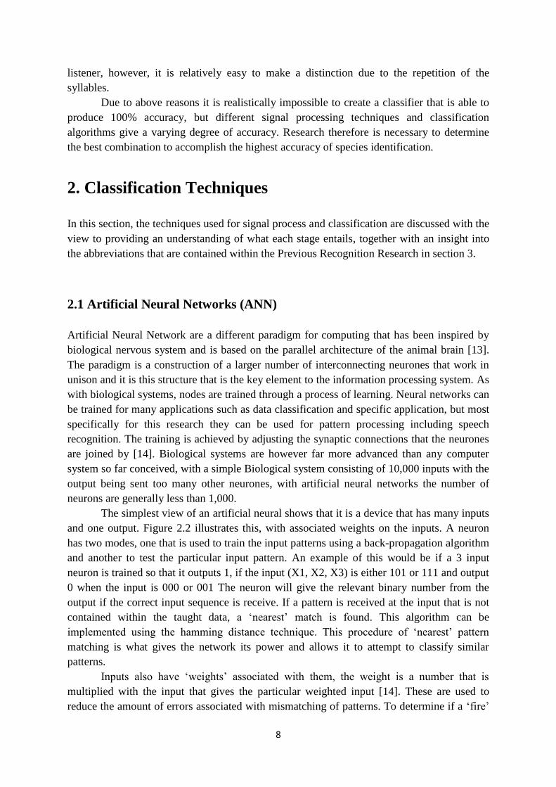
If the data is distributed too complexly it may not be able to be linearly separated in a
lower dimension, however, in a higher dimension it may be possible [1]. To accomplish a
separation of the data using a hyperplane in a higher dimension a hyperplane is constructed
halfway between the two data samples, this is chosen so the distance between the samples is
maximized [1].
Figure 2.3 shows a 2-dimentioanl space that is separated by a 1-dimentional hyperplane [16].
The figure is taken from [16].
Due to an SVM only being able to separate between two classes a method to overcome this a
method was conceived to allow the classifier to accomplish recognition on larger datasets. This is
achieved by creating multiple SVMs which are able to do large scale recognition. There are two
methods of this occurring. Either an SVM is constructed for every class, with the other class data
being a combination of all the other classes combined. Or two classes are represented by a single
SVM and a hierarchy is then constructed. Recognition is enabled by deciding which is the right class
is.
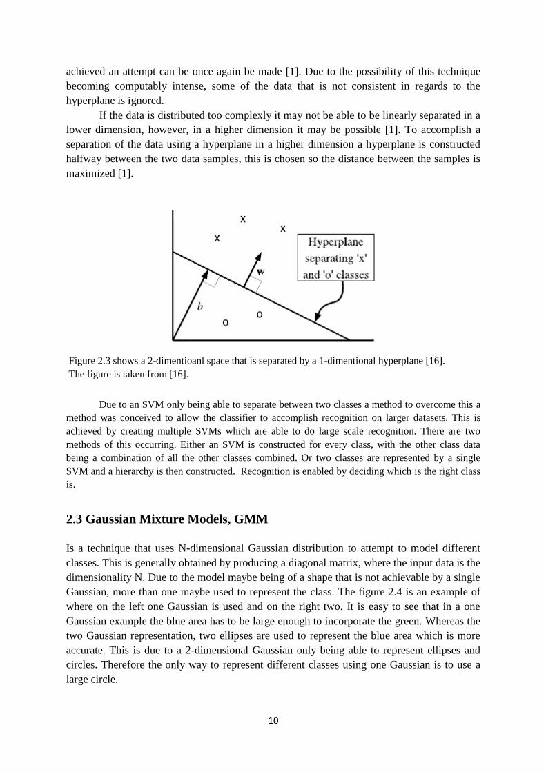
2.3 Gaussian Mixture Models, GMM
Is a technique that uses N-dimensional Gaussian distribution to attempt to model different
classes. This is generally obtained by producing a diagonal matrix, where the input data is the
dimensionality N. Due to the model maybe being of a shape that is not achievable by a single
Gaussian, more than one maybe used to represent the class. The figure 2.4 is an example of
where on the left one Gaussian is used and on the right two. It is easy to see that in a one
Gaussian example the blue area has to be large enough to incorporate the green. Whereas the
two Gaussian representation, two ellipses are used to represent the blue area which is more
accurate. This is due to a 2-dimensional Gaussian only being able to represent ellipses and
circles. Therefore the only way to represent different classes using one Gaussian is to use a
large circle.
11
Figure 2.4 is an example of 2D models, on the left shows data that is being modelled using one
Gaussian and on the right 2 Gaussians [1]. Figure is taken from [1].
K-clustering is used to initialize the GMM when training it with N mixtures, this is
due to not knowing which data points belong to which mixture [1]. Once this has been
completed, training by Expectation-Maximization (EM) can begin. The process of training a
GMM involves creating a model for every class. The class that creates the highest probability
by computing the average probabilities of all frames enables recognition.
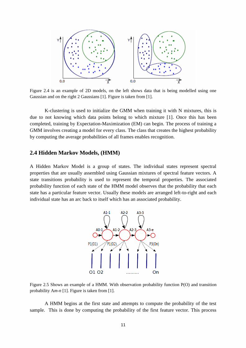
2.4 Hidden Markov Models, (HMM)
A Hidden Markov Model is a group of states. The individual states represent spectral
properties that are usually assembled using Gaussian mixtures of spectral feature vectors. A
state transitions probability is used to represent the temporal properties. The associated
probability function of each state of the HMM model observes that the probability that each
state has a particular feature vector. Usually these models are arranged left-to-right and each
individual state has an arc back to itself which has an associated probability.
Figure 2.5 Shows an example of a HMM. With observation probability function P(O) and transition
probability Am-n [1]. Figure is taken from [1].
A HMM begins at the first state and attempts to compute the probability of the test
sample. This is done by computing the probability of the first feature vector. This process
12
continues from one state to the next (which may be the same state) until all features of an
example are observed, computing the observation probabilities for each state as it goes [1].
Figure 2.5 is an example of a 3 state HMM with the beginning point and end point visible.
The probability for a state going to the next state is Am-n. This is due to all models only
having one begin state. The possibility of this state moving to the first state due to it only
having one arc is A0-1 which is 1. The probability of the state moving to another state via an
arc is the sum of 1. Within a simple model the probability of getting to the end state is 0. This
does not hold true if the HMM comprised of several smaller HMMs, in this case, the
probability of getting to the end state is not necessarily 0 [1].
To be able to assign every feature vector to the right state causes a problem. To
overcome this, a trellis is constructed, with the possible state on the y-axis and the feature
vectors on the other. The possible moves when using a left-to-right model is either by moving
right or by moving diagonal (right and upwards). Taking this onboard, an optimal path is then
deducted, by starting in the bottom left hand corner and finishing in the top right. To be able
to accomplish this, the Viterbi algorithm is used [1].
Due to not knowing which feature vectors belong to which state training the model is
slightly harder. To overcome this problem the training samples are distributed amongst the N
states, with the first
being assigned to the first state and the second
being assigned to the
next and so forth for each of the training samples [1]. After this the data assigned to each
state is used to train the GMM of that state. Next, the Viterbi algorithm is used by iteratively
assigning the features vectors to states which enables the EM training. The data is used to
recalculate the transition probabilities by training the GMMs [1]. To accomplish recognition,
for every class a HMM is trained, the probability of the test samples is computed for each of
HMMs and then the highest probability of the test sample is assigned to the class of the
HMM [1].
2.5 Hybrid Systems
Other methods of recognition which combine the techniques such as HMM and ANN to
produce hybrid systems are also an option. Research into systems that incorporate the use of
hybrid HMM and ANN are well documented in automated speech recognition. These hybrid
techniques have shown to produce good results and higher accuracy compared to standard,
more conventional approaches. However there is little or no evidence of such a system being
applied to bird song recognition. Therefore, experiments on a hybrid system are to be
undertaken during this research to determine if the high accuracy results seen with human
speech recognition transpire with bird songs. A tandem connectionist methods will be
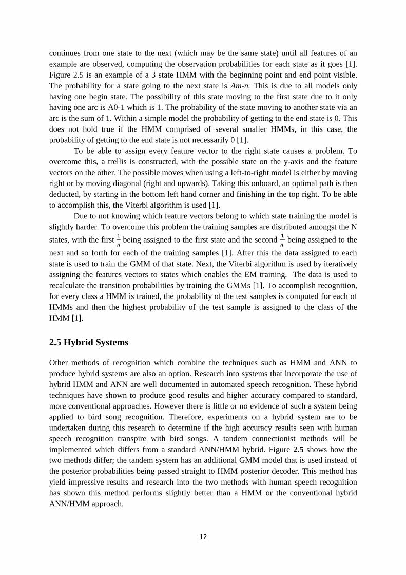
implemented which differs from a standard ANN/HMM hybrid. Figure 2.5 shows how the
two methods differ; the tandem system has an additional GMM model that is used instead of
the posterior probabilities being passed straight to HMM posterior decoder. This method has
yield impressive results and research into the two methods with human speech recognition
has shown this method performs slightly better than a HMM or the conventional hybrid
ANN/HMM approach.
13
The standard method for a hybrid ANN/HMM method would be to replace the GMM
of the HMM which is used to calculate the state probabilities with an ANN. The resulting
posterior probabilities would then be used as the state probabilities and the HMM models the
aspect of the speech.
Figure 2.5 shows the different approaches between a conventional hybrid ANN/HMM technique and
a tandem ANN/HMM model that will be used during this research.
However, the method used in this paper will not replace the GMM with an ANN instead the
GMM will remain and the HMM will be used in the conventional way. To begin with a
normal connectionist-HMM system is trained. To achieve this, a multilayered perception
neural network is trained to determine the posterior probabilities for each of the species.
Instead of using the probability stream as inputs to a HMM decoder as with a standard hybrid
ANN/HMM system, the output features are used as the features for the HTK (HMM toolkit).
Before the features are passed to the HTK the posterior probabilities are pre-processed due to
their skewed nature. This involves changing the features to the log domain. This gives the
features a more Gaussian distribution. After this the features dimensions are orthogonalized
by applying a Principal Component Analysis. Finally, the new features are added to the
original features to create tandem features. These features are then passed to the standard
HTK recognizer to be modelled by the Gaussian mixtures and standard HMM recognition
takes place.
Hybrid systems are seen as a good method to increase overall accuracy and provide a
good recognition technique. The method works well by reducing the disadvantages of the
HMM and ANN and combining the two methods to produce a technique that should
outperform the standard ANN or HMM methods.
3. Previous Recognition Research
The use of automated speaker recognition and its application to birdsong and other animal
recognition is under research and what there has been conducted is sparse. Generally much of
the work that is carried out does not build on previous work, which leads to difficulties when
comparing research. Much of the worked is based on researchers using their own classifiers,
feature sets and datasets. This section focuses on the research that has been undertaken in this
field. In particular, using models Artificial Neural Networks (ANN) and then Support Vector
Machines (SVM) to identify variations in the methods.
Following this, the commercial product SongScope and the previous work conducted
at The University of Sheffield will be discussed. This will help to continue the work that has
already been conducted. Other papers were reviewed for this project. However only those
selected are the best fit with regards to examining previous work conducted with SVM and
ANN classifiers. The relevance of these papers is described later.
14
3.1 McIlraith et al (1995)
In this paper the author attempts to produce a back-propagation neural network (ANN) that is
able to recognize bird songs [9]. This was attempted by using vocalisations which comprised
of 133 songs from six different bird species.
The pre-processing was undertaken by using a Linear Predictive Coefficient (LPC)
and Fast Fourier Transform (FFT). The data was end pointed by hand using the software
package Hypersignal plus [9]. The temporal information of the data was not taken into
consideration. A non-overlapping Hammering window which had 256 samples was used to
produce the framing. An LPC of each frame using 16 time domain coefficients was used [9].
The 16 LPC coefficients were used to construct a FFT with 9 unique spectral magnitudes.
The procedure was later repeated using a 1024 sample window.
Further work was carried out to determine the overall length of the actual vocalisation
as it is was believed to be a significant prompt in determining the identification of the
species. The addition of this variable helped the network to determine the vocalisation
through this hint [9]. The time variables were set to a standard deviation of one, with a mean
of zero [9] using a logistic function.
The classifier was able to correctly recognize around 80 to 85% of the samples
assessed. The data set which included a 256 sample window outperformed that which
contained 1024, with the mean sum-of-square errors being smaller and larger respectively for
the training data.
It was found that some of the species had bimodal frequency distributions, which lead
to songs consistently being misidentified. This was often due to the data sets used. Another
issue arose from using data that was obtained from the internet, which lead to
misclassification due to different dialects of the birds being used. This paper was written in (1995) and shows a very early attempt of trying to use an
ANN classifier and if it was possibility to use the classifier to recognise birdsongs. The
relative success of this work is difficult to determine due to the small dataset, lack of
comparative classification model and the lack of temporal information being used.
Additionally, the use of the songs length being used to help determine the species is neither
practical in a real-time situation nor productive in terms of determining the relative success
which makes the results relatively artificial. There are however, some positives to be gleaned;
the 256 sample window size outperformed the larger 1024 which indicates that the smaller
size is better and more importantly that working with an ANN is an effective process.
3.2 Cia et al (2010)
The paper by Cia et al uses an artificial neural network (ANN) for bird song recognition.
During this paper an investigation into the different methods of pre-processing techniques
was undertaken and the effects different feature sets have on recognition. Generally the
consensus when applying ANN to the bird recognition problem is to use frame based features
as inputs; frames are used to divide a song into even sized segment which enables recognition
through comparison of the test and training data. But the paper argues that it is too difficult to
model the dynamic process of the song with this approach [12]. Therefore, they decided that
15
to overcome this problem, frames from the “past” and “future” would be incorporated into
the current frame as inputs into the neural networks [12] and therefore construct a context
window. Three different data sets were used to carry out the experiment; these consisted of
audio files collected from subtropical rainforests, backyards and Australian subtropical east.
The data set contained 14 species, which should equate to a sizable dataset and good results.
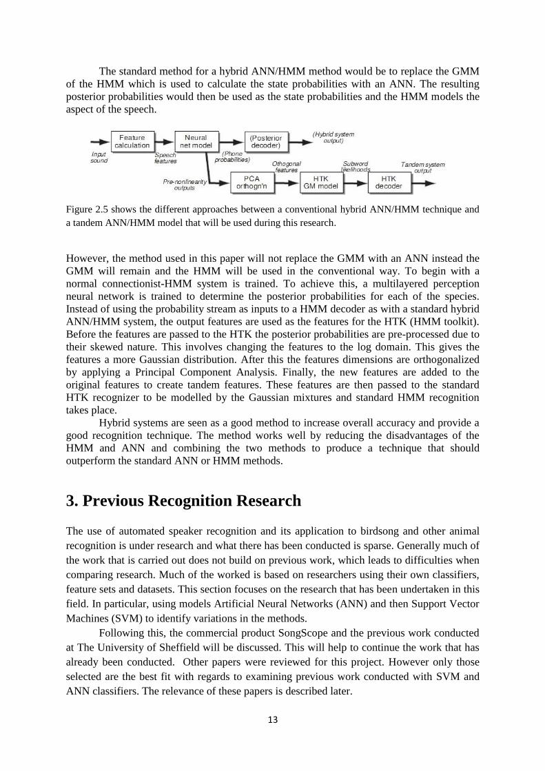
The author created their own noise reduction algorithm, in an attempt to reduce the
background noise levels, and figure 3.2 illustrates how this differs from a standard noise
reduction filter, for instance a wiener filter. The approach differs from other algorithms in
that the first few frames are usually taken as only containing noise and this is how the initial
background noise estimation is obtained [12]. This approach is generally used in speech
processing and due to the device being able to be calibrated to the background noise with the
speaker cooperation. However, applying this algorithm to birdsong is not as straight forward,
when applied in an environment where conditions are constantly changing. This makes it
difficult to estimate the background noise. The algorithm that was created does not need a
period of silence to obtain the background estimation and gives estimation from any frame.
This algorithm is compared to a minimum mean square error (MMSE) noise reduction filter
which is a standard noise filter that is used during speech processing.
The main feature extraction was done using an adapted Mel-Frequency Cepstral
Coefficient (MFCCs) and also linear scale cepstral coefficients, which are the same as a
MFCC but without the Mel-scale conversion. The comparison was taken to determine the
effectiveness of the Mel-scale conversion on the features.
Figure 3.2 shows signal enhancement (a) a traditional MMSE. (b) is there new method without SAD
[12]. The figure is taken from [12].
For the main classifier, a multilayer perception neural network (MLP NNs) was used.
Generally this approach when applied to the bird song recognition frame-based features are
used as the inputs to the MLP NN. This however causes problems due to it being difficult to
remove the temporal features from the frames [12]. To overcome this problem two techniques
were used. Differential features (Figure 3.3) which are used to model the difference between
neighbour features and time delay neural networks that take information from the current as
well as the “past” features. For the classification 13 coefficients are used for each frame as a
feature vector. For the time delay, 5 vectors are used at input and the output consists of three
16
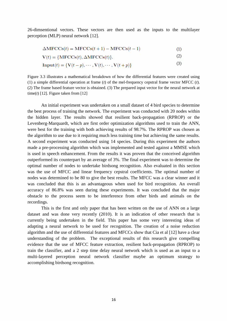
26-dimsentional vectors. These vectors are then used as the inputs to the multilayer
perception (MLP) neural network [12].
Figure 3.3 illustrates a mathematical breakdown of how the differential features were created using
(1) a simple differential operation at frame (t) of the mel-frequency cepstral frame vector MFCC (t).
(2) The frame based feature vector is obtained. (3) The prepared input vector for the neural network at
time(t) [12]. Figure taken from [12]
An initial experiment was undertaken on a small dataset of 4 bird species to determine
the best process of training the network. The experiment was conducted with 20 nodes within
the hidden layer. The results showed that resilient back-propagation (RPROP) or the
Levenberg-Marquardt, which are first order optimization algorithms used to train the ANN,
were best for the training with both achieving results of 98.7%. The RPROP was chosen as
the algorithm to use due to it requiring much less training time but achieving the same results.
A second experiment was conducted using 14 species. During this experiment the authors
made a pre-processing algorithm which was implemented and tested against a MMSE which
is used in speech enhancement. From the results it was proven that the conceived algorithm
outperformed its counterpart by an average of 3%. The final experiment was to determine the
optimal number of nodes to undertake birdsong recognition. Also evaluated in this section
was the use of MFCC and linear frequency cepstral coefficients. The optimal number of
nodes was determined to be 80 to give the best results. The MFCC was a clear winner and it
was concluded that this is an advantageous when used for bird recognition. An overall
accuracy of 86.8% was seen during these experiments. It was concluded that the major
obstacle to the process seem to be interference from other birds and animals on the
recordings.
This is the first and only paper that has been written on the use of ANN on a large
dataset and was done very recently (2010). It is an indication of other research that is
currently being undertaken in the field. This paper has some very interesting ideas of
adapting a neural network to be used for recognition. The creation of a noise reduction
algorithm and the use of differential features and MFCCs show that Cia et al [12] have a clear
understanding of the problem. The exceptional results of this research give compelling
evidence that the use of MFCC feature extraction, resilient back-propagation (RPROP) to
train the classifier, and a 2 step time delay neural network which is used as an input to a
multi-layered perception neural network classifier maybe an optimum strategy to
accomplishing birdsong recognition.
17
3.3 Ross (2006)
The goal of this thesis was to classify audio files of ten bird species using Artificial Neural
Network (ANN), Support Vector Machine (SVM) and Kernel Density Estimation (KDE)
models. The project had two main goals, firstly to evaluate the performance of the three
pattern recognition algorithms and secondly, due to previous works focusing on the long-term
global characteristics; to research if short-term tonal qualities are sufficient for distinguishing
bird species. Therefore, all recordings were selected on their merit due to short-term
characteristics and global ones were ignored.
All recordings were digitized at 44.1 kHz, and recordings that were more resistant to
background noise were selected over those that were not. The signals were then segmented
into 512 frames those that were classified as noisy frames or silent frames were discarded by
setting a high discrimination threshold. By finding the optimal point on the receiver operating
characteristics (ROC) curve [16]. Three sets were then created from the 160712 frames that
were created from the 512 audio files. The three sets comprised of training, test and cross-
validation data.
The three compilers consist of an ANN model that was hand coded using GNU C++,
and explanation for the back-propagation algorithm was provided by Haykin (1994). The
model comprised of three layers; the input layer, the hidden layer and output layer [16]. For
the output layer linear neurones were used and the hidden layer the logistic neurones were
used. A varied number of training epochs, learning rates and hidden nodes were used to
determine the best configuration.
The LIBSVM was used for the SVM model. Due to the SVM being an inherently
binary classifier a work around was used for a “one-against-one” approach. This is achieved
by training k(k-1)/2 classifiers for each class pair. The classifier therefore “votes” for a class
and the result is taken as the winner. This approach was chosen as a result of the work of
Chang and Lin (2005) because the data trained quicker.
Finally the KDE, as stated, is by far the easiest algorithm of the three, taking the form
of a single formula. A multivariate normal kernel (KRF) is used and gives the formula. The
classifier was hand coded in C++.
After the classification had taken place, two methods of post-processing was used to
establish the species. These were simple voting, which determined the output vector by the
maximum element by using simple voting mechanism that determines the winner. Secondly,
confusion matching which works in a similar way to simply voting but after the call has been
processed is used, and a confusion matrix is constructed; the vote tally forms a single row
from the matrix, or a confusion row. The matrix is used to determine the closet match to the
species by probabilities.
For the models ANN and SVM three different configurations were used per model,
but for the KDE only one was used. For the ANN 20, 100 and 500 were used. These
represented the amount of nodes. The SVM configurations were FAR, MID and NEA which
were parameters that corresponded to far, midrange and near in relation to the grid search.
From the results, it is shown that the ANN-500 has signs of overtraining with the training
score at 98%, but had lower test score than those of the ANN-100.The ANN scored in the
region of 64-67%, All three of the SVM results are within 5% of each other, with the SVM-
18
MID scoring slightly better. The KDE significantly scored worse out of all the classifiers
obtaining a score of 40%. The overall best performer was the ANN-100 with an average of
82% accuracy. From the post-processing results, both the systems had a similar average
accuracy with the chi-test slightly increasing with the weaker classifiers.
The paper by Ross [16] is the first and only example of an ANN and SVM being
compared to one another. The results showed that an ANN outperformed the SVM classifier
on all tests including the configurations which showed signs of overtraining. This paper
described an expectable way of constructing a SVM using a simple technique of comparing
two species.
3.4 Fagerlund (1997)
In this paper, Fagerlund [6] studies the use of bird vocalisation to determine the specie. This
is done by using two representations, descriptive signal parameters and Mel-Frequency
Cepstral Coefficient (MFCCs), to undertake recognising syllables of birdsong. A Support
Vector Machine (SVM) algorithm that depends on a decision tree and nearest neighbour are
used to perform the classification [6]. The test data consists of two sets; one with 6 birds and
another with 8.
To conduct the initial preparation of the recordings, an iterative time domain
algorithm was applied to the samples. This was used to estimate the background noise level
by computing the smooth energy envelope and then the energy of the signal was set to the
minimum. The initial threshold was set to half this amount, and once this is achieved an
iterative algorithm is run to determine the syllables with anything above this threshold,
updating the estimation from the average energy from the gaps between the syllables and
setting it to half this amount. The solution is obtained by running the algorithm recursively
until it converges on a solution. [1].
MFCCs with first derivatives and MFCCs with first and second derivatives and
descriptive parameters are utilized for the features; these are similar to those used by
Fagerlund [6]. The two data sets were manually segmented into syllables and separated into
test and training subsets, syllables would only appear in one or the other sets.
To train the support vector machines a pyramid setup was used which allows two
birds to be compared to one and other. The actual training utilised the sequential minimal
optimization (SMO) algorithm which was implemented to train the individual classifiers, this
was done using the support vector toolkit in MATLAB.
A mixture of the descriptive feature and the MFCC features were used across the two
datasets to gain the recognition results. Four different representations of the SVM were used.
Each syllable is treated by the SVM as a new sample. The Mahalanobis distance measure
was used to classify the nearest neighbour which was compared to the MFCC features
method. The reference implementation and the descriptive parameters fared worse than that
of the SVM classifier with the combination of the MFCC representation. The best results
were obtained using the method that used a mixture of all features. Again, with the second
dataset the mixture method performed somewhat better, with all classifiers relatively
equivalent.
19
The experiments here showed that using an SVM classifier works well with MFCCs.
This evidence supports the general consensus that the MFCC is the optimum algorithm for
signal processing. The use of Matlab and the support vector machine toolkit (LIBSVM)
seems an ideal solution to train and create the SVM model for classification. Once again
however, this work uses syllable extraction and does not make use of temporal information.
3.5 Arogant (Song Scope) (2009)
This project focuses on the commercial product Song Scope, which is the only licensed
software that claims to be able to undertake birdsong recognition from their vocalisations [1].
This research details the development of the software and how it accomplishes its real-time
identification. The algorithm is of a general HMM with feature vectors that are similar to Mel
Frequency Cepstral Coefficients (MFCCs), which is effective, robust and has been adapted to
be used for bird songs [2].
SongScope makes use of several techniques to reduce the noise created by automatic
remote monitoring systems by first pre-processing the audio signal (SongScope). Initially, a
wiener filter is applied to the signal, which reduces the stationary background noise. To
enable the filter to be able to perform this reduction a simple one-second rolling calculation is
produced to determine the spectrum that preceded the previous FFT window. With this
approach a large proportion of the high frequency background noise is removed and also
helps to reduce the low frequency. The signal is then passed through a band-pass filter to
produce the second step of the noise filtering. This approach helps to reduce the interference
that occurs at the higher and lower frequency, including vehicle and wind noises which are
generally located at the lower end of the frequency. A good estimation of the background
noise can be determined by the power that is inversely proportional to the frequency. This is
stated as “pink noise”. The high-pass filter is applied at around 1 kHz - 8 kHz and simply
ignores frequencies outside this band. The next step is to redistribute the signal spectrum
from a linear frequency scale to a log frequency scale [2]. This is not directly done to reduce
noise but is similar to MFCCs used in speech transformation. The thesis describes how a Mel
scale with regards to human speech recognition is a logarithmic frequency scale which is
used to model the sensitivity of the human ear. However, SongScope uses a slightly different
approach by using spectral feature reduction to enable a spectral feature through log
frequency scale transformation rather than trying to model the hearing sensitivity of the
animal [2]. This is done under the assumption that the fundamental vocalisation frequencies
harmonics higher frequency components are redundant. The specific band-pass filter is an
adaptation of the actual log scale, according to the formula the log-spaced bin
is determined by the number of log frequency bins which derive from the band-pass filter and
equate to the number of linear frequency bins , and constant k. This value is determined
such that the original number of linear frequency bins equal the number of log frequency bins
included in the band-pass filter [1]. Finally, using the fixed dynamic range the log power
levels are normalised. The frequency bin with the highest energy level determines the equal
dynamic range. To enable this, the power level is taken of each frequency bin and shifting the
20
FFT window. If any of the bins normalised power is estimated to be less than the background
noise level, the bin is said to be zero. This significantly reduces interference noise.
Due to the test audio files obtaining more than one vocalisation, a detection algorithm
was needed, and this was done by monitoring the tonal energy that passed through the band-
pass filter [2]. To determine the local maximum and minimum energy, a rolling window of
length 2x (Max Syllable Duration + Max Syllable Gap Duration) was applied. Low and high
water marks were established, the low being at +12dB above the local minimum and the high
+6dB above that. A syllable is determined when the energy goes above the high water mark
and ends when it is lower than the low water mark. If the length of the vocalisation last
longer than a predetermined Max Syllable Length and an inter-syllable gap is detected, the
vocalisation is determined to be complete [2].
A HMM algorithm which uses GMMs for the individual states, are used to construct
the classifiers. A syllable level of recognition is used, with the individual syllables modelled
with the syntax of how these syllables form to create a vocalisation are taken into
consideration. The temporal information is taken into consideration using state transition
probabilities. A k-means cluster was used to group the syllables into similar syllables and
classes. Once these classes are made, the syllables are then sequentially added to the classes
with regards to the mean duration. A state is then created to represent the inter syllable gap.
This enables a Hidden Markov Model topology, with transition probabilities and Gaussian
mixtures to be refined and estimated with the Viterbi algorithm [2].
The results showed that the classifier was able to identify 63% of vocalisations on the
training data, with 95% representing at least one vocalisation detected for all target
recordings. The false positive rate for each classifier for the training data was 0.3%. For the
test data the classifier was able to obtain an average detection rate of 37%, with 74% of all
target recordings obtaining at least one vocalisation, with the false positive rate at 0.4% for
the test data [2].
Although this research gave relatively good results, it is hard to compare the performance of
the classifier to that of other algorithms due to only the SongScope algorithm being applied to
the data. As this research was conducted by Bioaustics Software (the SongScope creators),
using a dataset that was created by themselves as an intended marketing tool, it maybe that
these results are slightly fabricated. However, due to SongScope being the only commercial
product available their product can be used as a viable benchmark.
3.6 Departmental Work
A look at other work conducted in the University Of Sheffield Department Of Computer
Science.
3.6.1 Brown et al (2009)
During this Darwin Project, Brown et al compared three models that were created using
methods, DTW, SVM and GMM. These were then compared to the commercial product
SongScope. Data was collated from the internet from freely available resources that had been
21
produced by amateurs. The recording consisted of 608 samples of 5 different species. The
recordings were manually processed to remove any background noise and interference from
the recordings.
The data was then divided into two equal sets of data, one being used for training and
the other for testing. The features from both sets were then extracted. The SVM and GMM
was tested upon the whole song, however for the DTW syllables extraction was used. The
data was divided into frames to calculate the features with 265 samples. The Direct Cosine
Transform and Fast Fourier Transform (FFT) of these features were calculated and computed
respectively. To remove the data that was insignificant, energy that was lower than one tenth
its maximum strength was removed.
The syllables for the DTW were divided into clusters using the k-means clustering
technique, the minimizing intracluster distance and the maximising intercluster distance
determined the amount of clustering. Experimentally it was determined that the best approach
using five mixtures for GMM was seen as the best value. The SongScope data was annotated
in the SongScope environment [1].
Overall the results showed that, regarding accuracy, the GMM gained the best result
of 55.2%, with SongScope software slightly worst with 32%, SVM was third with an
accuracy of 23.8% and finally the worst performer the DTW at 10%. The SVM method took
a great deal longer to train and test although performed relatively poorly when compared to
the GMM and SongScope. The tests however, never tested the accuracy at syllable level of
either the SVM or GMM, although this level of syllable extraction was conducted by
SongScope internally as well as the DTW model.
The research conducted in this project showed that GMM classifier is able to
outperform that of Song Scope‟s HMM classifier. The tests however, never tested the
accuracy at syllable level of either the SVM or GMM. although this level of syllable
extraction was conducted by SongScope internally as well as the DTW model. This leaves a
situation whereby it is difficult to compare the relative successful of the classifiers against
each other. Additionally, the research was conducted on a material that was of varying quality
and of a single bird per recording.
3.6.2 Gelling (2010)
This project focuses on the use of GMM and HMM to determine which of the two
recognition models preformed best overall, and is therefore a continuation of previous work
undertaken by Brown et al [4]. The SongScope software was used as the basis for the HMM
classifier during this project, with the investigation of the significances of temporal
information upon recognition, with methods of feature extraction similar to SongScope
replicated.
The data set that was previously used by Brown et al [4], which has 602 samples
contained within 5 different species, was again used for the experiments. The software
program Matlab was used to extract the temporal syllables and additional pre-processing
procedures. The NetLab Toolkit which is contained within the software, was used to form
statistical models, k-means clustering algorithm was created with this toolkit which was used
22
in some of the experiment along with the GMM classifier. The Hidden Markov Toolkit
(HTK) was used to manipulate HMM Models.
As previously stated the process of feature extraction was similar to that undertaken
by SongScope. To extract the features from the recording, first a wiener filter was applied
with the background noise determined on the less energetic 0.25 seconds [1]. This is done by
applying a Fast Fourier Transform (FFT) to identify these least energetic parts, having non-
overlapping windows. The time bins are found, where the lowest bins at that time are the sum
of all frequency bin values. The parameters of the Wiener Filter are then estimated due to the
time bins in the FFT of the corresponding sections of the original audio files [1]. Once this is
done, the FFT is used to produce recordings with 8 milliseconds step sizes and 16
milliseconds window sizes (subsequently equivalent to the 50% overlap and 256 frames that
SongScope uses). The used window was the Hamming window [1]. From here a bandpass
filter was applied to the data, which removed all the frequency bins of frequencies over and
under, 10kHz and 900 Hz respectively. A Mel-frequency filterbank which was comparative
to that one used in SongScope as next applied; this version of a Mel-frequency filterbanks is
dissimilar to those generally used in automatic speech recognition (ASR) and relies on
rectangular filters.
The energies were normalised by converting the energies into decibels of the resulting
spectrum. At this stage a large amount of the background noise was removed by making the
highest energy to be set at 0dB. This enabled the removal of any time-frequency bins that
were recorded below -20dB to be set at -20dB [1]. The final stage was to pass the features
through a Direct Cosine Transformation. This was done by applying the previous stated
bandpass filter which consisted of 212 cepstral coefficient time-frames. The time-frames
each consisted of 212 cepstral coefficients using the above bandpass filter. After the
combined effects of the above stated, similar results of that achieved by SongScope are seen
[1]. The features are extracted from the data at this stage. To test the ability of the recogniser,
several different tests were conducted upon the data to determine the effects different
variables have on the accuracy of the classifiers. Below is a breakdown of the experiments
conducted by Gelling.
1 To decide the optimal combination of features and mixtures, a GMM was used to
make syllable-level recognition. One model for each species was created for each
syllable.
2 To evaluate the performance of the HMM which has different amounts of mixtures
and states, an experiment is conducted to see if an increase in accuracy can be
performed by obtaining temporal information within a syllable by modelling. The
expected results were that a GMM with the equivalent number of mixtures will
perform the same as a HMM using one state.
The next section of experiments requires that clustering of the syllables takes place; this was
done by using the k-means clustering algorithm after which they were grouped. Each cluster
23
is represented as a single HMM. This is used instead of modelling a single HMM for all
syllables of a species.
3 A HMM with one state was modelled as a GMM to determine the overall optimal
amount of clusters per species, was then examined to see if by adding more states a
higher accuracy could be obtained.
4 The GMM and HMM are tests to see if clustering can be used to gain performance
recognition on whole recordings and to what extent.
3.6.2.1 Experiments and Results
An initial test was undertaken to determine the best number of cepstral coefficients per frame
to be used. This was done because a normal MFCC used around 12 coefficients, but currently
the type of filter that was being used computed a cepstral coefficient of 212. So, to determine
the required amount, the remainder of the experiments were carried out using a GMM with 1
to 6 mixtures, with varying amount of features. It was determined through the experiments
that 12 represented the optimal number of coefficients needed to produce the best accuracy
and so this was used for the rest of the experiments.
Secondly, an experiment with HMM was used, but this time mixtures of 1 to 5 were
used with the number of states being the same. The HMM with one state was used as a
representation of a GMM because they are relatively equivalent. The results showed that
increasing the mixtures and states, up to a maximum of 5, generally increased the accuracy of
the results. The states and mixtures of 1 that were being used as a GMM equivalent out
performed that of the pure GMM. However, the extra states of the HMM clearly showed as a
superior classifier.
In the third experiment extraction of the features was used to determine if this process
is better than that of trying to classify upon the whole recording. As previous stated, a
clustering algorithm was applied to the syllables for each species. Increasing the number of
cluster per species was investigated to determine the optimal amount for accuracy. In all
experiments the number of states 3, mixtures 2 and coefficients 12 were used. This was so
that the model didn‟t experience over fitting. The number of models for a single species was
increased whilst the remainder were kept the same; this was done to find out the right amount
of models per species. It was found that increasing the number of clusters to a maximum of 5
gave marginally better results. Therefore, a final test was undertaken where the number of
clusters was set at 2 and the amount of mixtures and states varied between 1 to 5 [1]. It was
shown that the greater the number of states and mixtures again tended to increase the
accuracy.
The final experiment was to determine if using the whole recording obtained better
results. To train the models, syllables were extracted from the recording using the Viterbi
algorithm. One HMM model was used per species, as only the change in accuracy was
required to be recognised. Additionally, a silence model was made to remove any sections of
noise at the beginning and end of the audio files [1]. The results although not conclusive,
24
showed that using whole recording may increase the accuracy but not greatly. It is shown that
the mean average for 3 to 5 states is very similar.
The results are an improvement of those conducted by Brown et al [4], apparently due
to better pre-processing techniques which enabled a greater degree of background noise
extraction, and also due to the fact that the data was normalised and transformed into a log-
frequency. Additionally, the frequency range was reduced so that only the syllables were
contained. Without this process the system has addition data that may decrease the accuracy.
The observations were also compared to that achieved using SongScope, and this
highlighted that the results obtained for testing data was much lower than that achieved in
this paper. However, the data set used for SongScope was much larger and this greater
number of birds may have affected the results. Also, the research was carried out on much
longer recording, with one of the main goals being to reduce false-positives, which may have
affected the positive results.
The overall view of the paper is that although multiple HMM gave slightly better
results than those of the GMM and single HMM, the difference wasn‟t significantly
statistically different. It also showed that although temporal information increased the
accuracy of the overall results, this increase was marginal at best. It is believed that a larger
data set may show greater variations in the methods.
Due to some of this work been based on that conducted by Gelling [1], a large
breakdown of this work was undertaken, the work carried out here was. The experiment of
particular interested is the final one that was conducted. This experiment used whole
recording and will be similar to the procedure undertaken in the experiment conducted in this
project. The results here seem promising in that obtaining recognition from a whole recording
performed slightly better than the pre-processing technique and classifier code that was
produced during this thesis will be incorporated in the research that is conducted here and is
discussed later.
3.7 Literature Discussion
As previously described, the area of song birdsong is relatively under researched. The papers
discussed in section 3.1 are the full extent of the published work that is obtainable in research
of ANN and SVM classifiers. Much of the work focuses on the use of syllable extraction to
test and train the data with the work conducted upon a small corpus, with temporal
information consistently not being taken into consideration. Much of this work was
undertaken to determine the effectiveness of the relevant techniques rather than attempting to
apply the research to the actual problem of recognising species through birdsongs. With the
exception of Cia et al [12]. It has also been found that syllable matching is not scalable to a
large set of species, especially if several highly variable narrowband vocalisations are
integrated into the mix [2] However, much of this research illustrates the signal processing
and classification techniques that are useful and adaptable to larger sets.
In the next section 3.2, was a look at research undertaken by SongScope and was
included into this review due to it being one of the only papers conducted on a large corpus.
Since SongScope is the only commercial offering techniques to classify bird species, the
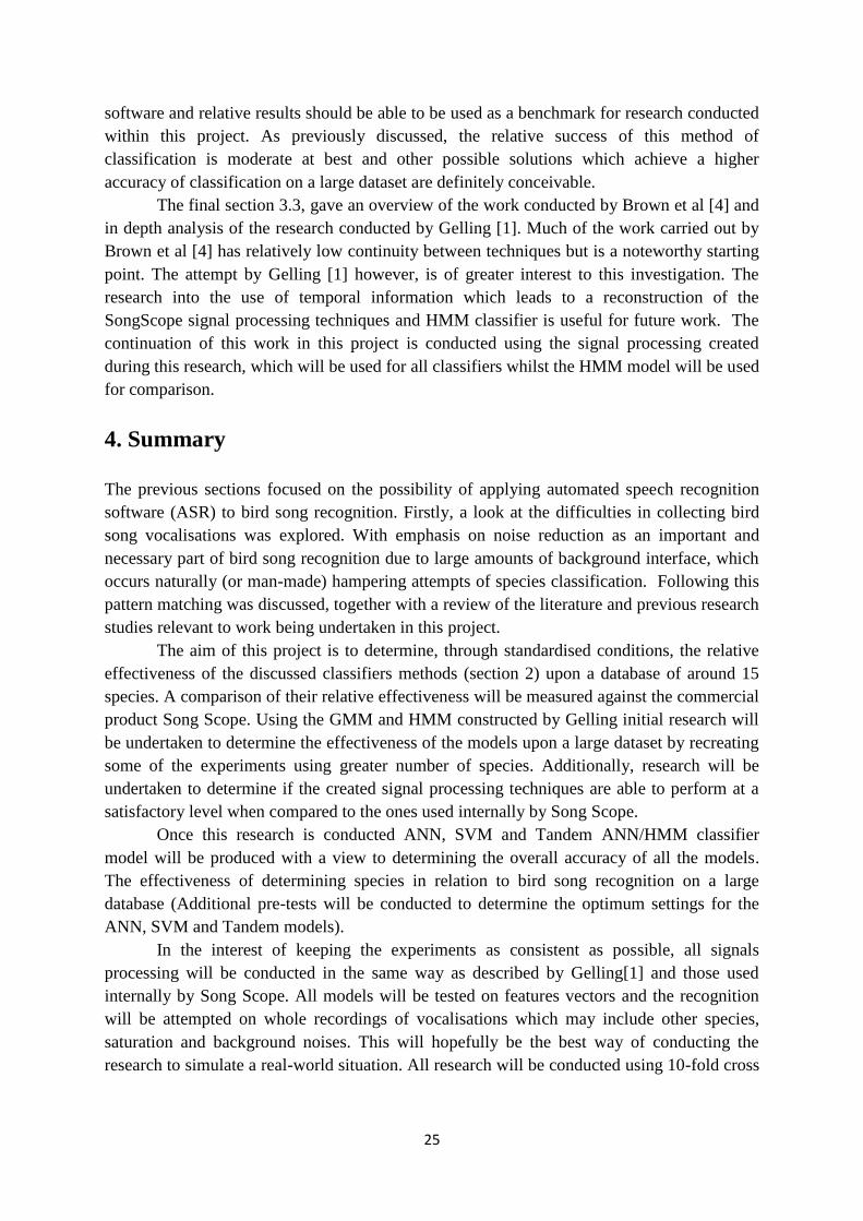
25
software and relative results should be able to be used as a benchmark for research conducted
within this project. As previously discussed, the relative success of this method of
classification is moderate at best and other possible solutions which achieve a higher
accuracy of classification on a large dataset are definitely conceivable.
The final section 3.3, gave an overview of the work conducted by Brown et al [4] and
in depth analysis of the research conducted by Gelling [1]. Much of the work carried out by
Brown et al [4] has relatively low continuity between techniques but is a noteworthy starting
point. The attempt by Gelling [1] however, is of greater interest to this investigation. The
research into the use of temporal information which leads to a reconstruction of the
SongScope signal processing techniques and HMM classifier is useful for future work. The
continuation of this work in this project is conducted using the signal processing created
during this research, which will be used for all classifiers whilst the HMM model will be used
for comparison.
4. Summary
The previous sections focused on the possibility of applying automated speech recognition
software (ASR) to bird song recognition. Firstly, a look at the difficulties in collecting bird
song vocalisations was explored. With emphasis on noise reduction as an important and
necessary part of bird song recognition due to large amounts of background interface, which
occurs naturally (or man-made) hampering attempts of species classification. Following this
pattern matching was discussed, together with a review of the literature and previous research
studies relevant to work being undertaken in this project.
The aim of this project is to determine, through standardised conditions, the relative
effectiveness of the discussed classifiers methods (section 2) upon a database of around 15
species. A comparison of their relative effectiveness will be measured against the commercial
product Song Scope. Using the GMM and HMM constructed by Gelling initial research will
be undertaken to determine the effectiveness of the models upon a large dataset by recreating
some of the experiments using greater number of species. Additionally, research will be
undertaken to determine if the created signal processing techniques are able to perform at a
satisfactory level when compared to the ones used internally by Song Scope.
Once this research is conducted ANN, SVM and Tandem ANN/HMM classifier
model will be produced with a view to determining the overall accuracy of all the models.
The effectiveness of determining species in relation to bird song recognition on a large
database (Additional pre-tests will be conducted to determine the optimum settings for the
ANN, SVM and Tandem models).
In the interest of keeping the experiments as consistent as possible, all signals
processing will be conducted in the same way as described by Gelling[1] and those used
internally by Song Scope. All models will be tested on features vectors and the recognition
will be attempted on whole recordings of vocalisations which may include other species,
saturation and background noises. This will hopefully be the best way of conducting the
research to simulate a real-world situation. All research will be conducted using 10-fold cross
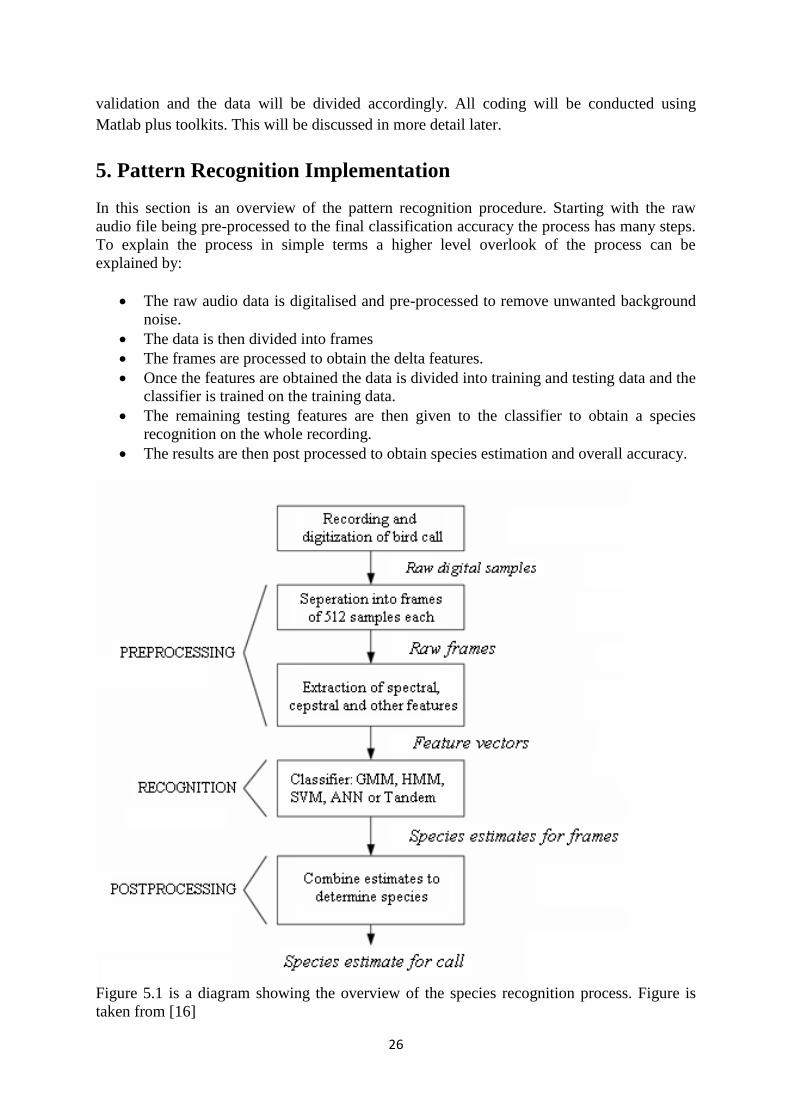
26
validation and the data will be divided accordingly. All coding will be conducted using
Matlab plus toolkits. This will be discussed in more detail later.
5. Pattern Recognition Implementation
In this section is an overview of the pattern recognition procedure. Starting with the raw
audio file being pre-processed to the final classification accuracy the process has many steps.
To explain the process in simple terms a higher level overlook of the process can be
explained by:
The raw audio data is digitalised and pre-processed to remove unwanted background
noise.
The data is then divided into frames
The frames are processed to obtain the delta features.
Once the features are obtained the data is divided into training and testing data and the
classifier is trained on the training data.
The remaining testing features are then given to the classifier to obtain a species
recognition on the whole recording.
The results are then post processed to obtain species estimation and overall accuracy.
Figure 5.1 is a diagram showing the overview of the species recognition process. Figure is
taken from [16]
27
5.1 Data and Bird Species
To begin with the raw data has to be sourced. Previous research undertaken by the
department has been carried out on a small data set that comprised of around 600 recording
samples containing 5 species which had been obtained freely from the internet. However
Gelling [1] concluded that this dataset was too small to obtain meaningful results. A larger
amount of data was therefore sourced via Mauro Nicolao who is a PHD student at The
University of Sheffield. The data has been collected from a region in Northern Italy by local
researchers in the area.
The data consists of recordings sampled at a rate of 48.1kHz and are recorded in
stereo. The database consisted of raw data recordings of around 6 minutes or longer
containing many different songs and calls. The data has had labels added to the recordings by
the research team using the program Praat. The data is labelled in three layers: protected
species, common species and noise and disturbing events. The protected species consists of
around 10 species and 80-170 audio files for each bird. Each file is around 2 to 60 seconds
duration, with the majority of the birds songs of a non-structured nature, many of these
species are larger birds of prey. The common species consists of about 22 different bird
species from the Northern-Italy area, with around 50 or more audio files per species (more
could be obtained through labelling of the data). There is a high variation of song duration
with some as long as 3 minutes, with most of these birds using a real structure vocalisation.
The noise and disturbance events consist of wind, microphone saturation, aeroplanes and
disturbance caused by overlapping birds. This data could be used to create a disturbance
classifier.
Due to research being conducted by the Italian research team on population density of
the protected species data containing the birds calls have already been extracted by the
researchers and a subset of shorter recordings has been made. This is the data that will be
used for the experiments conducted in this paper, this is due to the time consuming nature of
species song extraction and also the Italian researcher‟s abilities to identify different species.
Additionally to this, due to the data being obtained from Italy it has been an issue
transporting the data.
Due to the data set only containing 10 species the Brown et al [4] data, which contains
5 species, will be added to the data to created a dataset that contains 15 species. Below is a
list of the species that are contained within the dataset, the number of recordings per species
and average recording length.
Species Amount of Recordings Mean Recording Length
Bananaquit 115
1.88
Black Grouse 144
16.04
Black Woodpecker 125
5.75
Boreal Owl 88
14.97
Ferruginous Owl 61
6.98
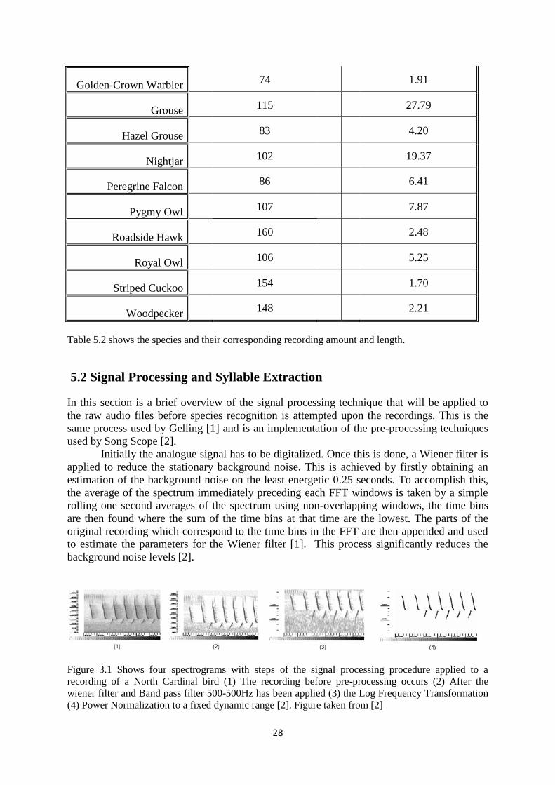
28
Golden-Crown Warbler 74
1.91
Grouse 115
27.79
Hazel Grouse 83
4.20
Nightjar 102
19.37
Peregrine Falcon 86
6.41
Pygmy Owl 107
7.87
Roadside Hawk 160
2.48
Royal Owl 106
5.25
Striped Cuckoo 154
1.70
Woodpecker 148
2.21
Table 5.2 shows the species and their corresponding recording amount and length.
5.2 Signal Processing and Syllable Extraction
In this section is a brief overview of the signal processing technique that will be applied to
the raw audio files before species recognition is attempted upon the recordings. This is the
same process used by Gelling [1] and is an implementation of the pre-processing techniques
used by Song Scope [2].
Initially the analogue signal has to be digitalized. Once this is done, a Wiener filter is
applied to reduce the stationary background noise. This is achieved by firstly obtaining an
estimation of the background noise on the least energetic 0.25 seconds. To accomplish this,
the average of the spectrum immediately preceding each FFT windows is taken by a simple
rolling one second averages of the spectrum using non-overlapping windows, the time bins
are then found where the sum of the time bins at that time are the lowest. The parts of the
original recording which correspond to the time bins in the FFT are then appended and used
to estimate the parameters for the Wiener filter [1]. This process significantly reduces the
background noise levels [2].
Figure 3.1 Shows four spectrograms with steps of the signal processing procedure applied to a
recording of a North Cardinal bird (1) The recording before pre-processing occurs (2) After the
wiener filter and Band pass filter 500-500Hz has been applied (3) the Log Frequency Transformation
(4) Power Normalization to a fixed dynamic range [2]. Figure taken from [2]
29
A FFT that consists of a window size of 16 milliseconds and step size of 8
milliseconds (which corresponds to a 256 frames and 50% overlap) is next applied to the
recordings, the window that is used is the hamming window. Once this is achieved the power
spectrum is obtained and band-pass filter is applied. [1]. This is done to reduce the
interference cause by other sounds that are contained within the recording in higher or lower
frequencies (above 10KHz and below 900Hz) than the range the bird vocalisations occur. The
frequencies were obtained manually by determining the highest and lowest frequency to
which the bird vocalisations lie. This helps to eliminate other sounds such as wind and rain.
After the band-pass filter has been applied, the signal is shifted from a linear spectrum
to a log frequency scale. This however is not directly linked to noise reduction but is similar
to Mel Frequency transforms which is used in speech recognition. The Mel scale is a
logarithmic frequency and is designed to imitate the sensitively of the human ear, assuming
that spectral features are likely to correspond to specific frequencies of the human ear [2].
However, to model the sensitivity of bird hearing the log frequency scale transformation is
used for spectral feature reduction and this is done by assuming that the higher frequency
components are redundant harmonics of the fundamental vocalisation frequencies [2]. To
achieve this a filter bank similar to Mel-frequency filter banks is applied but with rectangular
filters. The boundaries for the individual filters in the filterbank are described by the function:
[1]
The resulting spectrum is then normalised, the energies are converted to decibels by
setting the highest energy to 0dB. Any time bins that fall below -20dB are set to -20dB which
dramatically reduces the amount of background noise. This process is undertaken on a per
recording basis and therefore the maximum energy is recalculated separately for each
recording. Finally a Direct Cosine Transform (DCT) is applied to the features. The resulting
features contain 212 cepstral coefficients. This is achieved by applying the bandpass filter
mentioned earlier [1]. This process should drastically reduce the background noise, as seen in
Figure 3.1 example (4).
To obtain the syllables that are required to train the classifiers, a method similar to
that is used by Fagerlund et al [5] implemented. The normalised features are used as the base
data to extract the syllables before the Direct Cosine Transform (DCT) is applied. The data is
transformed back into the power spectrum and for every time bin the average frequency bins
are taken. The resulting vectors are smoothed by convoluting the vectors with vectors of
ones, which have a length of nine. Some extra points are created at the beginning and the end
of each vector due to the convoluting process, but these are omitted. The remaining vectors
have the first and last 4 values removed and replaced by 0.01. This is done to remove the
steep slope that the vectors would have at this point, which would have a detrimental effect
on the syllable extraction process. The front and end of the recording are generally noise and
the value 0.01 on the power spectrum converts back to the original -20dB [1].
Finally the vectors are increased so that the maximum equates to 0 and the noise is
estimated to be the minimum value. The threshold is determined by multiplying the noise by
a factor of 0.9, which was obtained experimentally. This should allow for the syllables to be
extracted successfully but still allow the syllables to be separated properly. The noise for all
bins is iteratively recalculated for the bins that fall below the threshold and are updated as a
result. This continues until the algorithm converges, the periods that are higher than the
threshold and are longer than 3 frames are counted as containing a syllable [1].

30
6. Classification
For this research 6 different classifiers are used. These include a Gaussian Mixture Model
(GMM), Hidden Markov Model (HMM), Artificial Neural Network (ANN), Support Vector
Machine (SVM) and a Tandem ANN/HMM system. In section 2 the different methods are
discussed in depth, however in the section a look at the construction of the different
classifiers and the methods that are used.
6.1 Implementation and Toolkits
To be able to accomplish the species recognition an acceptable application and implementing
techniques were need to be sourced. The application and programming languages Matlab
was therefore used with additional toolkits as required. The pre-processing, syllable
extraction (which were described in section 5.2) and data manipulation are all achieved via
Matlab. Additionally to this, several Toolkits are used to aid the construction of the
classification algorithms with a couple of these contained within Matlab itself.
In regards to the GMM and HMM which had both been previously hand coded by
Gelling [1] and are to be used during these experiments. For the GMM the Matlab toolkit
Netlab was used, which provides an implementation to creating several statistical models
including Gaussian Mixture Models (GMM). For the HMM the toolkit HTK was used, this
toolkit is used to manipulate and build HMMs. This application is generally used for speech
recognition but has been applied to other form of recognition, including bird songs, which
makes it ideal for this research.
The next two models that are constructed are the ANN and SVM. Due to previous the
work being conducted within Matlab the obvious choose was to continue to use the software
for the remainder of the experiments. An investigation to see if the ANN and SVM classifiers
could be constructed using Matlab found that the robust programming language had both a
Neural network (ANN) and support vector machine (SVM) toolkits available. However on
closer inspection the SVM toolkit is only available to support binary condition so alternative
was sourced.
Therefore for the Support Vector Machines an alternative method was found. There
are two alternatives available, the LIBSVM is capable of regression, classification, supports
multi-classifications and distributed estimation. Whereas the SVMTorch is generally used to
solve classifications problems and large scale regression. After the research it was found that
LIBSVM library by Chang and Lin (2001) would be more suited due to there being available
LIBSVM Matlab source code and is therefore fully implementable within Matlab.
The final classifier to be made is that of a tandem ANN/HMM system which
incorporates both ANN and HMM. To enable construction of this design aspects of both the
HTK and Neural network toolkit where used.
The methods are discussed in more details in the next section.
6.2 Classifiers
6.2.1 Gaussian Mixture Model
A GMM classifier that was developed by Gelling [1] is used to conduct the experiments. The
model is constructed using the Netlab toolkit as previously stated. Gelling [1] describes how
the model works as follows:
31
To begin with the training data is pooled used to initialise a 1-mixture model on the
means and covariances of the training data. The mixture with the largest prior weight is then
split into two to obtain GMMs with more than one mixture. Each mixture is altered by the
proportion of the original variation in different directions. The model is then trained by
performing Expectation-Maximization six times. The final two steps are then repeated as
many times as necessary until the number of mixtures required is achieved. To perform
recognition, frame-by-frame voting is used to determine the average log probabilities for each
sample. The mixture model that obtains the highest probability is the model that is recognised
[1].
6.2.2 Hidden Markov Model
For the HMM, the model that was created by Gelling [1] using the HTK toolkit was used.
The following technique was implemented.
To begin with the tool is initialised by using the Hint (which is a function of the HTK
toolkit), this is done so that the training data can be segmented uniformly into files where
each state has a n/m feature vector assigned to it. Where the number of features vectors
within a training file is n and the amount of states is m. Due to the fact that only left-to-right
models are used to model the syllables, the groups are assigned one state at a time from left to
right. Beginning with state one, the state is assigned n/m feature sets. Then state two the
second n/m feature set and so on.
Once this is completed the GMM that is assigned to each set is then initialised, this is
achieved by clustering the data using the k-means clustering algorithm. The centres that are
produced are then used as the centres to the mixtures. To determine the covariances of the
mixtures the covariance data associated with each centre is used. The prior probability of a
centre is then initialised by using the proportion of the feature vectors associated with a
mixture relative to the number of feature vectors associated with a state [1].
The Viterbi algorithm is then used to segment the training data to perform
Expectation-Maximization training, through this process the GMM models that are associated
with the HMM states are updated. The training process is replicated until 20 Expectation-
Maximization passes have been performed or if the model converges.
To perform recognition the HVite tool is used. HVite uses the token pass algorithm to
do the Viterbi recognition. Recognition is then performed. The HMM network that is used
depends upon the grammar file [1].
6.2.3 Artificial Neural Network
To produce the ANN the Matlab Neural Network toolkit was used.
The network consists of three layers, the input layer, hidden layer and output layer.
For the hidden layer logistic neurons are used and for the output layer linear neurons. A
context window is created by making features that contain 5 feature vectors. This is done by
combining the two “before” feature vectors with the current feature as well as two “after”
feature vectors. Doing this enables the classifier to be trained on feature that contains
temporal information from the frames surrounding vectors. This should give better results
due to during training the ANN should be able to create more clearly defined neuron decision
boundaries.
To train the classifier resilient back propagation is implemented. This was favoured
over other methods for its ability to give good results but having a much quicker training time
than other methods. To determine the amount of training, a validation set was made from the
32
training data set by taking around 10% of the data. The RPROP was then used to epoch until
the training data converges on the validation set or if the number of epochs reached 1000,
whichever comes first. Once the network has been trained it is then used for recognition, to
achieve this test data is passed to the network and the posterior probabilities are obtained for
each frame of the recording. Finally frame-by-frame analysis is performed on the recording to
determine the overall species recognition.
6.2.4 Support Vector Machine
To implement the SVM the LIBSVM library by Chang and Lin (2001) was used.
The following options for the svm-train were used. These setting are the same as those
described by Ross [16].
The SVM is of the type C-SVC, or C-support vector classification.
The kernel is the radial basis function, ;
The internal cross-validation was set to five-fold.
The training algorithm that was used is the sequential minimal optimization (SMO).
The SVM is essentially a binary classifier. LIBSVM uses a “one-against-one” approach to get
around this. For each pair of classes, k(k-1)/2 classifiers are trained.
For the SVM therefore are two parameters that have to be altered to obtain an optimal
setting, this is done to gain the most accurate results. for the kernel, which in a normal
distribution is analogous to 1/ and the cost parameter C is the “penalty” value for
misclassifies points [16].To obtain these two variables LIBSVM-train has a build in cross-
validation function which determines the results by cross referencing many different
parameters until it determines the optimum settings for the data that is presented to it.
The prediction is obtained by each binary classifier “voting” for a class, the winner is
then taken to be the result. The results are obtained by using “frame-by-frame” voting. The
overall result for the recording is determined from the results from each frame [16].
6.2.5 Tandem System
To construct the Tandem HMM/ANN the HTK and neural network toolkits are used which
are constructed in Matlab. Both methods are used in similar to the way discussed earlier with
the standard HMM and ANN approach.
Firstly the features are processed and syllables are located and selected. Once the
syllables are known, a context window is produced for all the syllables. A context window
contains features that have information from 5 features vectors which included the two
“before” features, the current feature and two “after” features.
A conventional hybrid connectionist-HMM system is then trained using these new
features. This equates to a standard Multi-layer perception neural network being trained using
back propagation which is of the same construction as the standard artificial neural network
used in this research with one hidden layer. The estimations of the posterior probabilities that
33
the RPROP produces are obtained once the training of the ANN is completed. Because the
posterior probabilities have a skewed distribution they are warped into a different domain by
taking their logs. By doing this, the new log distributed features have a very unusual property
of containing one large value and several smaller values. Therefore principal component
analysis (PCA) is used to apply a global decorrelated which improves system performance.
The new features that have the same length as the number of species are combined with the
original feature vector to create tandem features. The tandem features are then passed to a
GMM-HMM based ASR which is used in the conventional way (see Hidden Markov Model
6.2.2).
To undertake recognition, the recognition data is passed through the ANN and the
posterior probabilities are obtained. The logged feature vectors are then decorrelated using
the principal component analysis statistics in simpler way to the training data. The new
features are then combined with the original features to create the tandem testing features.
These features are then passed to the HMM for decoding and the system performance can
then be measured.
7. Post processing
After the frames have been processed using the relative model a final interpretation of the
results has to done to determine the species. There are three separate methods used to
decipher the results. These are; frame-by-frame voting (used for the HMM, ANN and SVM),
Vertibi algorthim (used for HMM and the Tandem ANN-HMM system) and a confusion
matrix will be used for all methods to represent the data in a way so that the success of the
relative species can be determined. If there is any coloration between the models in which
species are miss respected in classification.
7.1 Frame-by-Frame Voting
The simplest of these methods is to implement a voting algorithm. The probabilities (or the
single digit result from the SVM) for each frame are analysis to determine which species has
been detected. At the end of each recording the result that was detected are added up and the
species with the most correct votes is determined to be the winner. Due to recognition
recordings being full length recordings without the vocalisations being removed, there is a
good chance that the highest recorded species is the silent model. If this is the case this is
ignored and the second highest vote is taken.
7.2 Viterbi Algorithm
This algorithm is used by the HMM (and the tandem ANN/HMM system) and is a method
used to decode a sequence of Markov observations by constructing a most likely path of
recognition through a matrix of probabilities. Or more simply the likely sequence of hidden
states. This process allows the HMM to be able to temporally determine the most likely
syllable sequence. The HMM in this process is able to recognise syllable sequences. This is
done by determining a syllable-silence-syllable sequence and uses the grammar file which
contains a list of bird syllables to determine the overall species.
34
7.3 Confusion Matrix
This method is similar to the frame-by-frame voting in the sense that incrimination is made
every time a corresponding species is found. Once the “votes” have been counted from a
species recording its results will become a confusion row or single row within a confusion
matrix. Once all the calls have been collated a matrix is formed that can be used to analysis
the data for any consistency regarding miss classification within the data. The correctly
identified species will lie on the horizontal of the matrix and from the experiments it should
be relatively easy to see miss classifications. It should make it easy to see if there is an
coloration between the classifiers and similar issues in regard to miss identification due to
false positives occur.
8. Experiments
As previously stated the experiments conducted by Gelling [1] will be repeated with a larger
amount of data. Experiments using the GMM and HMM classifiers will be assessed along
with the relative success rate of the ANN, SVM, the tandem HMM/ANN system and the
commercial software Songscope being used a s a benchmark. The experiments will be
conducted separately to determine the classifiers optional settings and an overall comparison
between the classifiers is to be made.
The data which was collated will be initially processed to perform feature extraction.
The process results in 212 cepstral coefficients being created per frame. This number is much
higher than the MFCCs used for automate speech recognition (which is around 12) therefore
a reduction of features will probably be necessary. Previous work conducted by Gelling [1]
showed that a reduction actually increased the HMM and GMM accuracy. The number of
features being used also has an effect on the processing time, with preliminary tests having
shown that reducing the number of coefficients significantly reduces the amount of time
required to process a large amount of data. Therefore an investigation into the optimum
number of features per model will be undertaken.
Experiments to determining the optimum setting for each of the models will use the
classifiers internal variables; for the GMM the number of mixtures will be used as the variant,
for the HMM the number of mixtures and states are experimental assed to attempt to optimise
performance, for the ANN the number of hidden states, for the SVM the kernel and cost
parameter and finally the tandem ANN/HMM system which has three variants; the number of
hidden states for the ANN and the number of mixtures and the number of states within the
HMM.
The experiment will be conducted using 10-fold cross validation (apart from SVM,
see section 6.2.4). The data recordings for each species are divided up randomly into 10
nearly equalled sized sets, with any remaining data being placed into the final set. Using the
syllables, which were identified earlier, the classifiers are then trained on 9 out of 10 of the
sets. Once trained the remaining roughly 10% of the data is used as the test set and the
classifier is tested. Once this has occurred the results are recorded and the process is repeated
10 times until all the sets have been tested on. The overall accuracy is then calculated by
taking the average accuracy from all the 10 results. The confusion matrix is created by adding
together all 10 confusion matrix together which gives an overall species recognition median
matrix. This process was used due to high results being obtained when the data was trained
on 90% of the data rather than another data split method. Also with obtaining 10 different
sets of results, the overall accuracy is a fairer estimation of the classifiers success by taking
an average rather than one possible ambiguous result.
35
All experiments are conducted by training and testing the classifiers on whole
recording. This is achieved by training the classifiers on the syllable obtained by using the
Fagerlund [5] method of syllable identification plus additional data from between the
syllables which is taken as the background noise and used as the silent model. The testing is
then achieved by given the classifiers the full recording for testing. The silent results were
then ignored for the final results. This was done because it is the method which is most
similar to how the techniques might actually be applied due to generally the data has not been
split into individual syllables in real world situations.
Finally, an assumption has to be made that all the data is normally distributed. Due to
the data being randomly distributed between the 10 sets it is a reasonable assumption. The
value for each set is therefore an approximation of the true accuracy, from a randomly
distribution which should have a true accuracy mean. For all test that are completed the
significance level will be set to 0.05 [1].
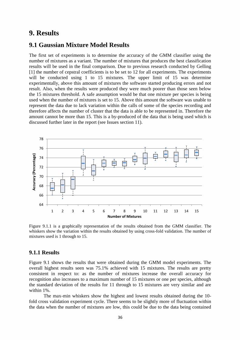
36
9. Results
9.1 Gaussian Mixture Model Results
The first set of experiments is to determine the accuracy of the GMM classifier using the
number of mixtures as a variant. The number of mixtures that produces the best classification
results will be used in the final comparison. Due to previous research conducted by Gelling
[1] the number of cepstral coefficients is to be set to 12 for all experiments. The experiments
will be conducted using 1 to 15 mixtures. The upper limit of 15 was determine
experimentally, above this amount of mixtures the software started producing errors and not
result. Also, when the results were produced they were much poorer than those seen below
the 15 mixtures threshold. A safe assumption would be that one mixture per species is being
used when the number of mixtures is set to 15. Above this amount the software was unable to
represent the data due to lack variation within the calls of some of the species recording and
therefore affects the number of cluster that the data is able to be represented in. Therefore the
amount cannot be more than 15. This is a by-produced of the data that is being used which is
discussed further later in the report (see Issues section 11).
Figure 9.1.1 is a graphically representation of the results obtained from the GMM classifier. The
whiskers show the variation within the results obtained by using cross-fold validation. The number of
mixtures used is 1 through to 15.
9.1.1 Results
Figure 9.1 shows the results that were obtained during the GMM model experiments. The
overall highest results seen was 75.1% achieved with 15 mixtures. The results are pretty
consistent in respect to: as the number of mixtures increase the overall accuracy for
recognition also increases to a maximum number of 15 mixtures or one per species, although
the standard deviation of the results for 11 through to 15 mixtures are very similar and are
within 1%.
The max-min whiskers show the highest and lowest results obtained during the 10-
fold cross validation experiment cycle. There seems to be slightly more of fluctuation within
the data when the number of mixtures are low, this could be due to the data being contained
64
66
68
70
72
74
76
78
1 2 3 4 5 6 7 8 9 10 11 12 13 14 15
Acc
ura
cy (
Pe
rce
nta
ge)
Number of Mixtures
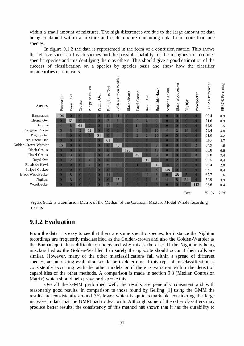
37
within a small amount of mixtures. The high differences are due to the large amount of data
being contained within a mixture and each mixture containing data from more than one
species.
In figure 9.1.2 the data is represented in the form of a confusion matrix. This shows
the relative success of each species and the possible inability for the recognizer determines
specific species and misidentifying them as others. This should give a good estimation of the
success of classification on a species by species basis and show how the classifier
misidentifies certain calls.
Species
Ban
anaq
uit
Bo
real
Ow
l
Gro
use
Per
egri
ne
Fal
con
Py
gm
y O
wl
Fer
rug
inou
s O
wl
Go
lden
-Cro
wn
War
ble
r
Bla
ck G
rou
se
Haz
el G
rou
se
Ro
yal
Ow
l
Ro
adsi
de
Haw
k
Str
iped
Cu
cko
o
Bla
ck W
ood
pec
ker
Nig
htj
ar
Wo
od
pec
ker
TO
TA
L P
erce
nta
ge
ER
RO
R P
erce
nta
ge
Bananaquit 104 0 0 0 0 0 11 0 0 0 0 0 0 0 0 90.4 0.9
Boreal Owl 0 63 0 0 0 2 6 0 9 6 2 0 0 0 0 71.6 0.9
Grouse 4 8 68 0 0 14 0 0 14 0 0 0 0 0 0 63.0 1.5
Peregrine Falcon 6 8 2 62 0 0 0 0 8 0 10 4 2 14 0 53.4 3.8
Pygmy Owl 4 0 0 8 64 0 4 0 2 2 16 0 5 0 0 61.0 8.2
Ferruginous Owl 0 0 0 0 0 61 0 0 0 0 0 0 0 0 0 100 4.7
Golden-Crown Warbler 16 0 0 0 0 0 48 0 0 0 8 0 0 0 2 64.9 1.6
Black Grouse 0 0 0 0 0 0 0 125 0 0 19 0 0 0 0 86.8 0.6
Hazel Grouse 0 3 0 5 0 4 0 0 49 0 6 8 0 0 8 59.0 3.4
Royal Owl 0 2 0 4 0 0 0 0 0 98 0 0 2 0 0 92.5 0.4
Roadside Hawk 0 0 0 4 0 6 12 0 1 0 112 14 2 8 0 70.4 2.8
Striped Cuckoo 0 0 0 0 0 0 0 0 0 0 6 148 0 0 0 96.1 0.4
Black WoodPecker 0 8 0 0 0 11 0 0 0 12 6 0 88 5 0 67.7 1.6
Nightjar 0 3 0 0 0 0 25 0 0 0 8 4 8 54 0 52.9 3.9
Woodpecker 0 0 0 0 0 2 3 0 0 0 0 0 0 0 143 96.6 0.4
Total 75.1% 2.3%
Figure 9.1.2 is a confusion Matrix of the Median of the Gaussian Mixture Model Whole recording
results
9.1.2 Evaluation
From the data it is easy to see that there are some specific species, for instance the Nightjar
recordings are frequently misclassified as the Golden-crown and also the Golden-Warbler as
the Bannanaquit. It is difficult to understand why this is the case. If the Nightjar is being
misclassified as the Golden-Warbler then surely the opposite should occur if their calls are
similar. However, many of the other misclassifications fall within a spread of different
species, an interesting evaluation would be to determine if this type of misclassification is
consistently occurring with the other models or if there is variation within the detection
capabilities of the other methods. A comparison is made in section 9.8 (Median Confusion
Matrix) which should help prove or disprove this.
Overall the GMM performed well, the results are generally consistent and with
reasonably good results. In comparison to those found by Gelling [1] using the GMM the
results are consistently around 3% lower which is quite remarkable considering the large
increase in data that the GMM had to deal with. Although some of the other classifiers may
produce better results, the consistency of this method has shown that it has the durability to
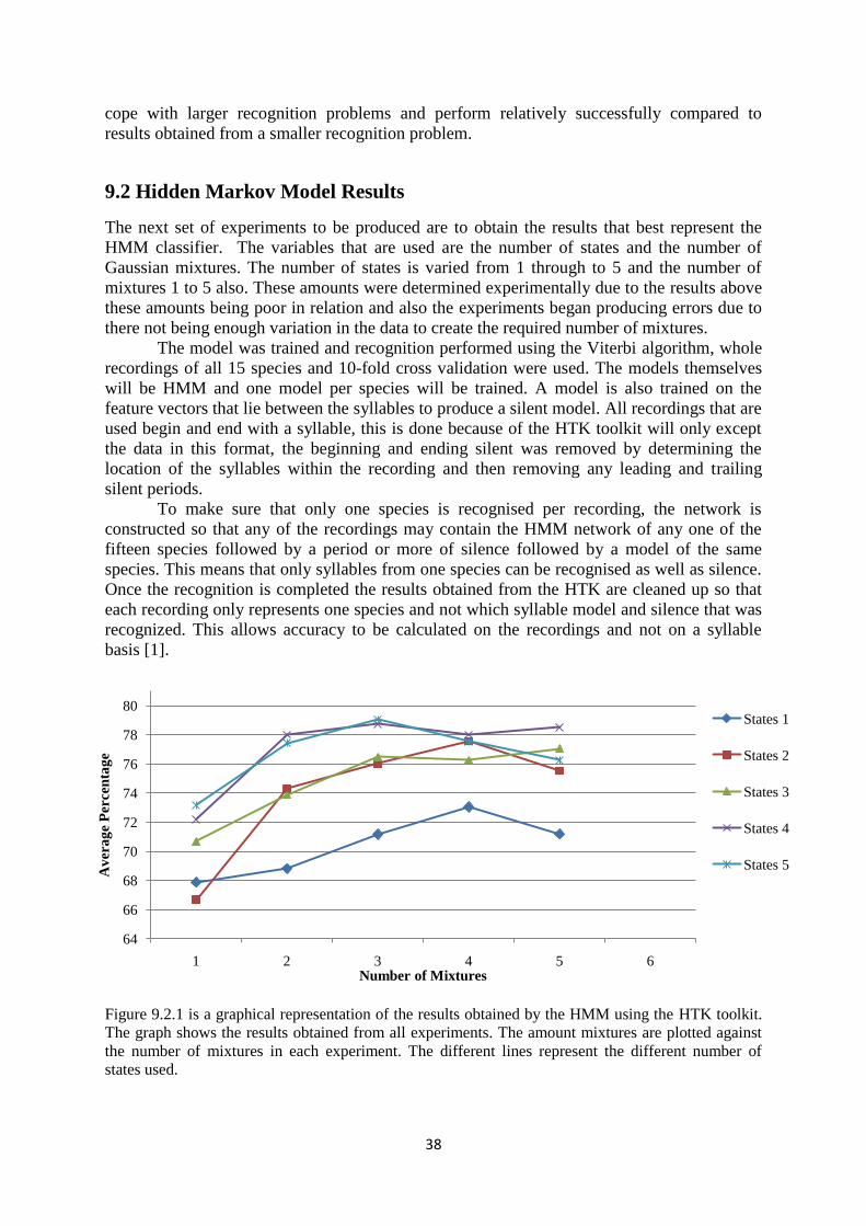
38
64
66
68
70
72
74
76
78
80
1 2 3 4 5 6
Av
era
ge
Per
cen
tag
e
Number of Mixtures
States 1
States 2
States 3
States 4
States 5
cope with larger recognition problems and perform relatively successfully compared to
results obtained from a smaller recognition problem.
9.2 Hidden Markov Model Results
The next set of experiments to be produced are to obtain the results that best represent the
HMM classifier. The variables that are used are the number of states and the number of
Gaussian mixtures. The number of states is varied from 1 through to 5 and the number of
mixtures 1 to 5 also. These amounts were determined experimentally due to the results above
these amounts being poor in relation and also the experiments began producing errors due to
there not being enough variation in the data to create the required number of mixtures.
The model was trained and recognition performed using the Viterbi algorithm, whole
recordings of all 15 species and 10-fold cross validation were used. The models themselves
will be HMM and one model per species will be trained. A model is also trained on the
feature vectors that lie between the syllables to produce a silent model. All recordings that are
used begin and end with a syllable, this is done because of the HTK toolkit will only except
the data in this format, the beginning and ending silent was removed by determining the
location of the syllables within the recording and then removing any leading and trailing
silent periods.
To make sure that only one species is recognised per recording, the network is
constructed so that any of the recordings may contain the HMM network of any one of the
fifteen species followed by a period or more of silence followed by a model of the same
species. This means that only syllables from one species can be recognised as well as silence.
Once the recognition is completed the results obtained from the HTK are cleaned up so that
each recording only represents one species and not which syllable model and silence that was
recognized. This allows accuracy to be calculated on the recordings and not on a syllable
basis [1].
Figure 9.2.1 is a graphical representation of the results obtained by the HMM using the HTK toolkit.
The graph shows the results obtained from all experiments. The amount mixtures are plotted against
the number of mixtures in each experiment. The different lines represent the different number of
states used.
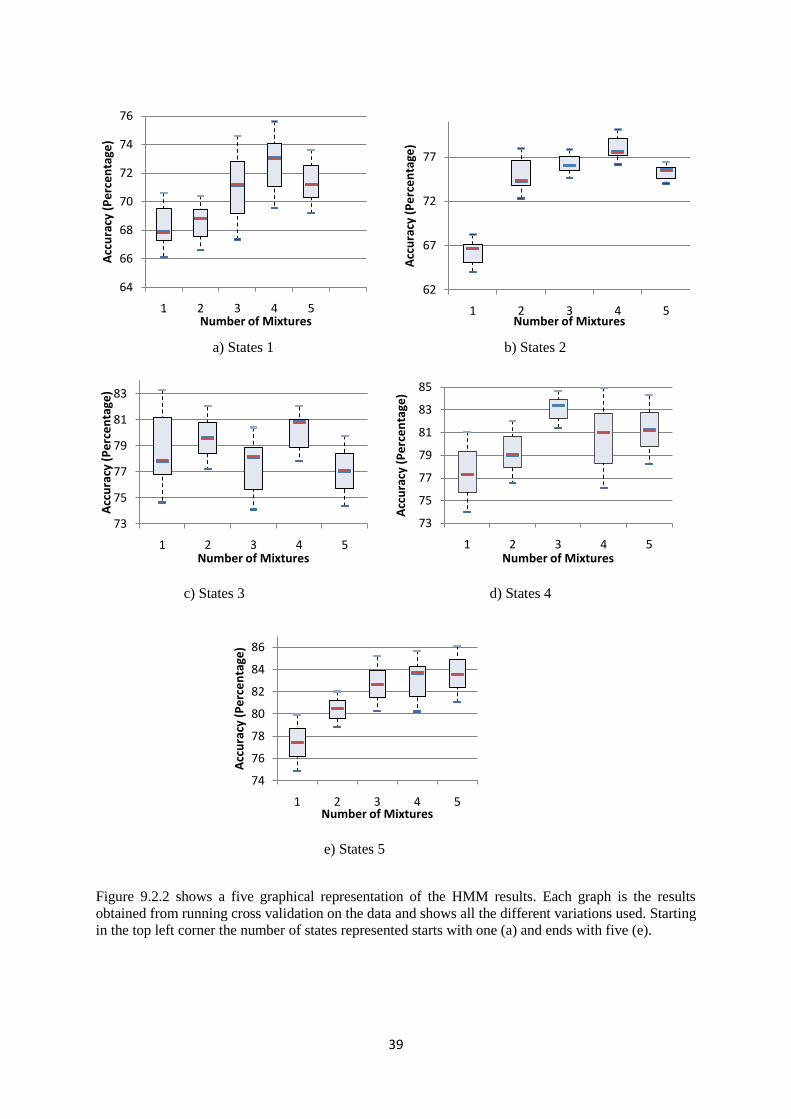
39
64
66
68
70
72
74
76
1 2 3 4 5
Acc
ura
cy (
Pe
rce
nta
ge)
Number of Mixtures
62
67
72
77
1 2 3 4 5
Acc
ura
cy (
Pe
rce
nta
ge)
Number of Mixtures
a) States 1 b) States 2
c) States 3 d) States 4
e) States 5
Figure 9.2.2 shows a five graphical representation of the HMM results. Each graph is the results
obtained from running cross validation on the data and shows all the different variations used. Starting
in the top left corner the number of states represented starts with one (a) and ends with five (e).
73
75
77
79
81
83
1 2 3 4 5
Acc
ura
cy (
Pe
rce
nta
ge)
Number of Mixtures
73
75
77
79
81
83
85
1 2 3 4 5
Acc
ura
cy (
Pe
rce
nta
ge)
Number of Mixtures
74
76
78
80
82
84
86
1 2 3 4 5
Acc
ura
cy (
Pe
rce
nta
ge)
Number of Mixtures
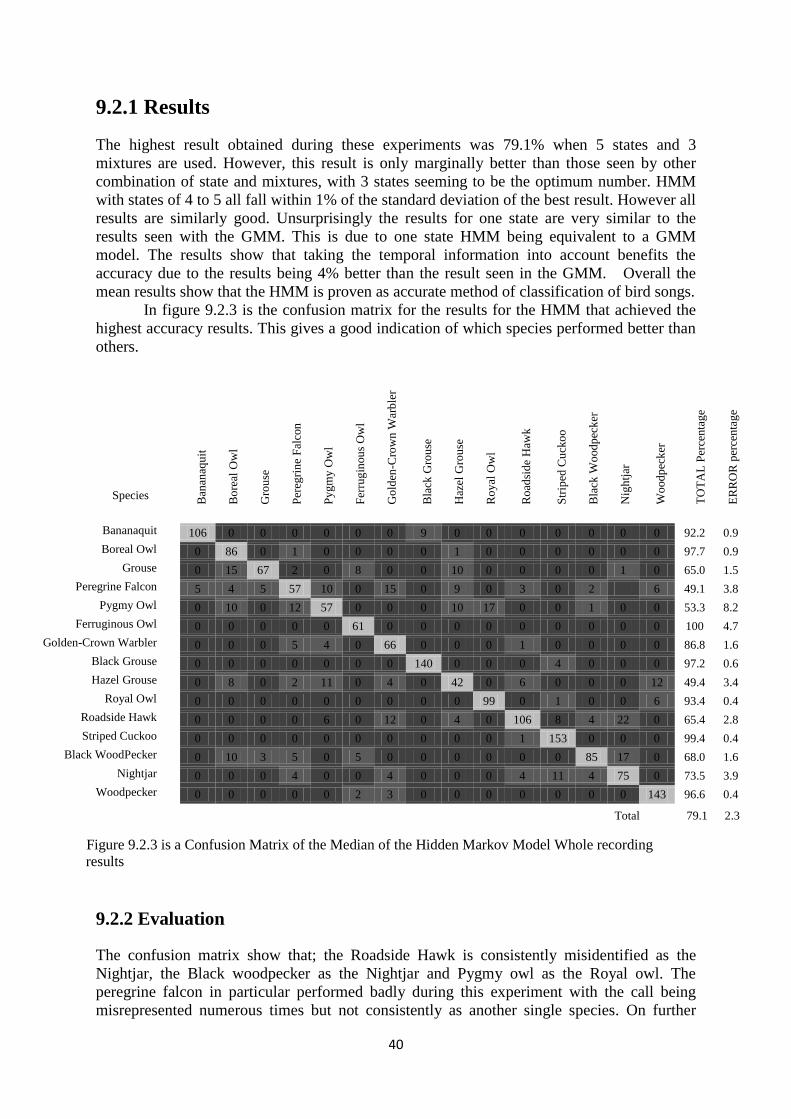
40
9.2.1 Results
The highest result obtained during these experiments was 79.1% when 5 states and 3
mixtures are used. However, this result is only marginally better than those seen by other
combination of state and mixtures, with 3 states seeming to be the optimum number. HMM
with states of 4 to 5 all fall within 1% of the standard deviation of the best result. However all
results are similarly good. Unsurprisingly the results for one state are very similar to the
results seen with the GMM. This is due to one state HMM being equivalent to a GMM
model. The results show that taking the temporal information into account benefits the
accuracy due to the results being 4% better than the result seen in the GMM. Overall the
mean results show that the HMM is proven as accurate method of classification of bird songs.
In figure 9.2.3 is the confusion matrix for the results for the HMM that achieved the
highest accuracy results. This gives a good indication of which species performed better than
others.
Species
Ban
anaq
uit
Bo
real
Ow
l
Gro
use
Per
egri
ne
Fal
con
Py
gm
y O
wl
Fer
rug
inou
s O
wl
Go
lden
-Cro
wn
War
ble
r
Bla
ck G
rou
se
Haz
el G
rou
se
Ro
yal
Ow
l
Ro
adsi
de
Haw
k
Str
iped
Cu
cko
o
Bla
ck W
ood
pec
ker
Nig
htj
ar
Wo
od
pec
ker
TO
TA
L P
erce
nta
ge
ER
RO
R p
erce
nta
ge
Bananaquit 106 0 0 0 0 0 0 9 0 0 0 0 0 0 0 92.2 0.9
Boreal Owl 0 86 0 1 0 0 0 0 1 0 0 0 0 0 0 97.7 0.9
Grouse 0 15 67 2 0 8 0 0 10 0 0 0 0 1 0 65.0 1.5
Peregrine Falcon 5 4 5 57 10 0 15 0 9 0 3 0 2 6 49.1 3.8
Pygmy Owl 0 10 0 12 57 0 0 0 10 17 0 0 1 0 0 53.3 8.2
Ferruginous Owl 0 0 0 0 0 61 0 0 0 0 0 0 0 0 0 100 4.7
Golden-Crown Warbler 0 0 0 5 4 0 66 0 0 0 1 0 0 0 0 86.8 1.6
Black Grouse 0 0 0 0 0 0 0 140 0 0 0 4 0 0 0 97.2 0.6
Hazel Grouse 0 8 0 2 11 0 4 0 42 0 6 0 0 0 12 49.4 3.4
Royal Owl 0 0 0 0 0 0 0 0 0 99 0 1 0 0 6 93.4 0.4
Roadside Hawk 0 0 0 0 6 0 12 0 4 0 106 8 4 22 0 65.4 2.8
Striped Cuckoo 0 0 0 0 0 0 0 0 0 0 1 153 0 0 0 99.4 0.4
Black WoodPecker 0 10 3 5 0 5 0 0 0 0 0 0 85 17 0 68.0 1.6
Nightjar 0 0 0 4 0 0 4 0 0 0 4 11 4 75 0 73.5 3.9
Woodpecker 0 0 0 0 0 2 3 0 0 0 0 0 0 0 143 96.6 0.4
Total 79.1 2.3
Figure 9.2.3 is a Confusion Matrix of the Median of the Hidden Markov Model Whole recording
results
9.2.2 Evaluation
The confusion matrix show that; the Roadside Hawk is consistently misidentified as the
Nightjar, the Black woodpecker as the Nightjar and Pygmy owl as the Royal owl. The
peregrine falcon in particular performed badly during this experiment with the call being
misrepresented numerous times but not consistently as another single species. On further
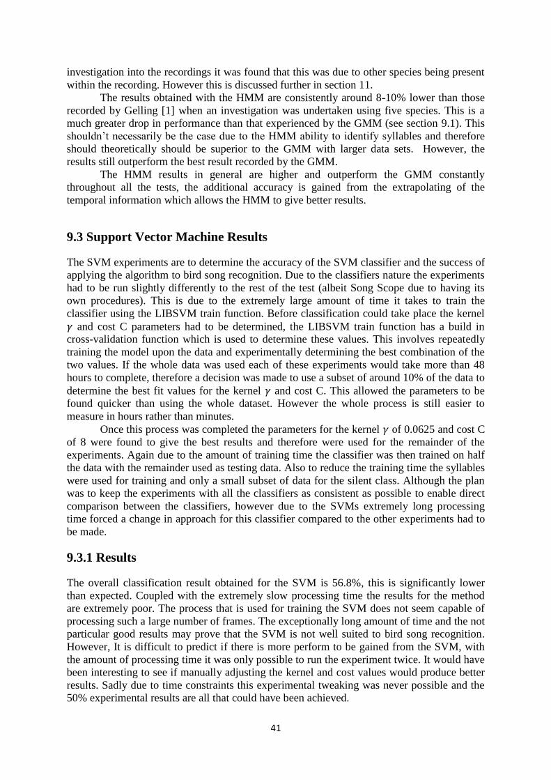
41
investigation into the recordings it was found that this was due to other species being present
within the recording. However this is discussed further in section 11.
The results obtained with the HMM are consistently around 8-10% lower than those
recorded by Gelling [1] when an investigation was undertaken using five species. This is a
much greater drop in performance than that experienced by the GMM (see section 9.1). This
shouldn‟t necessarily be the case due to the HMM ability to identify syllables and therefore
should theoretically should be superior to the GMM with larger data sets. However, the
results still outperform the best result recorded by the GMM.
The HMM results in general are higher and outperform the GMM constantly
throughout all the tests, the additional accuracy is gained from the extrapolating of the
temporal information which allows the HMM to give better results.
9.3 Support Vector Machine Results
The SVM experiments are to determine the accuracy of the SVM classifier and the success of
applying the algorithm to bird song recognition. Due to the classifiers nature the experiments
had to be run slightly differently to the rest of the test (albeit Song Scope due to having its
own procedures). This is due to the extremely large amount of time it takes to train the
classifier using the LIBSVM train function. Before classification could take place the kernel
and cost C parameters had to be determined, the LIBSVM train function has a build in
cross-validation function which is used to determine these values. This involves repeatedly
training the model upon the data and experimentally determining the best combination of the
two values. If the whole data was used each of these experiments would take more than 48
hours to complete, therefore a decision was made to use a subset of around 10% of the data to
determine the best fit values for the kernel and cost C. This allowed the parameters to be
found quicker than using the whole dataset. However the whole process is still easier to
measure in hours rather than minutes.
Once this process was completed the parameters for the kernel of 0.0625 and cost C
of 8 were found to give the best results and therefore were used for the remainder of the
experiments. Again due to the amount of training time the classifier was then trained on half
the data with the remainder used as testing data. Also to reduce the training time the syllables
were used for training and only a small subset of data for the silent class. Although the plan
was to keep the experiments with all the classifiers as consistent as possible to enable direct
comparison between the classifiers, however due to the SVMs extremely long processing
time forced a change in approach for this classifier compared to the other experiments had to
be made.
9.3.1 Results
The overall classification result obtained for the SVM is 56.8%, this is significantly lower
than expected. Coupled with the extremely slow processing time the results for the method
are extremely poor. The process that is used for training the SVM does not seem capable of
processing such a large number of frames. The exceptionally long amount of time and the not
particular good results may prove that the SVM is not well suited to bird song recognition.
However, It is difficult to predict if there is more perform to be gained from the SVM, with
the amount of processing time it was only possible to run the experiment twice. It would have
been interesting to see if manually adjusting the kernel and cost values would produce better
results. Sadly due to time constraints this experimental tweaking was never possible and the
50% experimental results are all that could have been achieved.
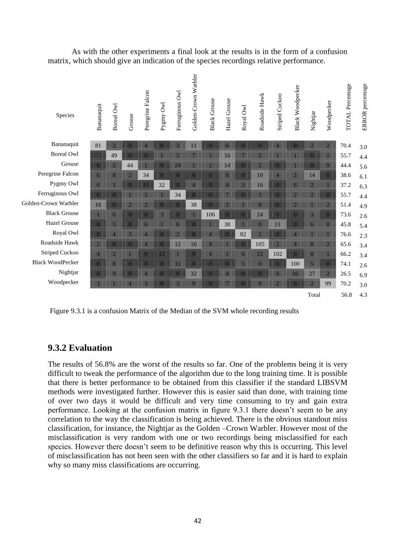
42
As with the other experiments a final look at the results is in the form of a confusion
matrix, which should give an indication of the species recordings relative performance.
Species
Ban
anaq
uit
Bo
real
Ow
l
Gro
use
Per
egri
ne
Fal
con
Py
gm
y O
wl
Fer
rug
inou
s O
wl
Go
lden
-Cro
wn
War
ble
r
Bla
ck G
rou
se
Haz
el G
rou
se
Ro
yal
Ow
l
Ro
adsi
de
Haw
k
Str
iped
Cu
cko
o
Bla
ck W
ood
pec
ker
Nig
htj
ar
Wo
od
pec
ker
TO
TA
L P
erce
nta
ge
ER
RO
R p
erce
nta
ge
Bananaquit 81 2 0 4 0 3 11 0 6 0 0 4 0 2 2 70.4 3.0
Boreal Owl 49 0 0 1 2 7 1 16 7 2 1 1 0 1 55.7 4.4
Grouse 0 2 44 1 0 24 1 1 14 0 2 0 1 0 9 44.4 5.6
Peregrine Falcon 6 8 2 34 0 0 0 0 8 0 10 4 2 14 0 38.6 6.1
Pygmy Owl 6 1 0 11 32 0 4 0 4 3 16 0 6 2 1 37.2 6.3
Ferruginous Owl 6 0 1 5 1 34 0 0 7 0 3 0 2 2 0 55.7 4.4
Golden-Crown Warbler 16 0 2 2 0 0 38 0 2 1 8 0 2 1 2 51.4 4.9
Black Grouse 1 6 0 0 3 0 1 106 0 0 24 0 0 3 0 73.6 2.6
Hazel Grouse 0 5 0 6 1 6 0 1 38 1 0 11 0 6 8 45.8 5.4
Royal Owl 0 4 3 4 0 2 0 4 0 82 2 0 4 1 1 76.6 2.3
Roadside Hawk 2 0 0 4 0 12 16 4 1 0 105 2 4 8 2 65.6 3.4
Striped Cuckoo 4 2 1 0 12 1 0 4 1 6 12 102 0 8 1 66.2 3.4
Black WoodPecker 0 8 0 0 0 11 0 0 0 5 6 0 100 5 0 74.1 2.6
Nightjar 0 9 0 4 0 0 32 0 4 0 0 8 16 27 2 26.5 6.9
Woodpecker 3 1 4 3 0 3 9 0 7 0 8 2 0 2 99 70.2 3.0
Total 56.8 4.3
Figure 9.3.1 is a confusion Matrix of the Median of the SVM whole recording results
9.3.2 Evaluation
The results of 56.8% are the worst of the results so far. One of the problems being it is very
difficult to tweak the performance of the algorithm due to the long training time. It is possible
that there is better performance to be obtained from this classifier if the standard LIBSVM
methods were investigated further. However this is easier said than done, with training time
of over two days it would be difficult and very time consuming to try and gain extra
performance. Looking at the confusion matrix in figure 9.3.1 there doesn‟t seem to be any
correlation to the way the classification is being achieved. There is the obvious standout miss
classification, for instance, the Nightjar as the Golden –Crown Warbler. However most of the
misclassification is very random with one or two recordings being misclassified for each
species. However there doesn‟t seem to be definitive reason why this is occurring. This level
of misclassification has not been seen with the other classifiers so far and it is hard to explain
why so many miss classifications are occurring.
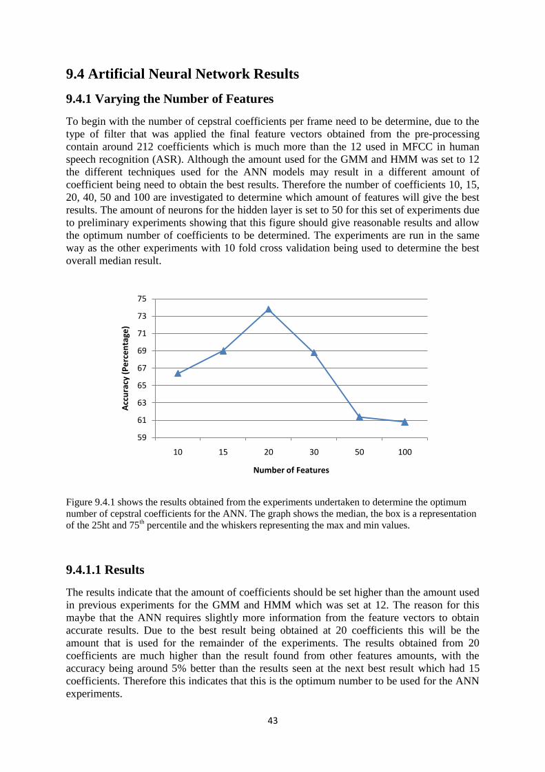
43
9.4 Artificial Neural Network Results
9.4.1 Varying the Number of Features
To begin with the number of cepstral coefficients per frame need to be determine, due to the
type of filter that was applied the final feature vectors obtained from the pre-processing
contain around 212 coefficients which is much more than the 12 used in MFCC in human
speech recognition (ASR). Although the amount used for the GMM and HMM was set to 12
the different techniques used for the ANN models may result in a different amount of
coefficient being need to obtain the best results. Therefore the number of coefficients 10, 15,
20, 40, 50 and 100 are investigated to determine which amount of features will give the best
results. The amount of neurons for the hidden layer is set to 50 for this set of experiments due
to preliminary experiments showing that this figure should give reasonable results and allow
the optimum number of coefficients to be determined. The experiments are run in the same
way as the other experiments with 10 fold cross validation being used to determine the best
overall median result.
Figure 9.4.1 shows the results obtained from the experiments undertaken to determine the optimum
number of cepstral coefficients for the ANN. The graph shows the median, the box is a representation
of the 25ht and 75th percentile and the whiskers representing the max and min values.
9.4.1.1 Results
The results indicate that the amount of coefficients should be set higher than the amount used
in previous experiments for the GMM and HMM which was set at 12. The reason for this
maybe that the ANN requires slightly more information from the feature vectors to obtain
accurate results. Due to the best result being obtained at 20 coefficients this will be the
amount that is used for the remainder of the experiments. The results obtained from 20
coefficients are much higher than the result found from other features amounts, with the
accuracy being around 5% better than the results seen at the next best result which had 15
coefficients. Therefore this indicates that this is the optimum number to be used for the ANN
experiments.
59
61
63
65
67
69
71
73
75
10 15 20 30 50 100
Acc
ura
cy (
Pe
rce
nta
ge)
Number of Features
44
9.4.2 Varying the Number of Hidden Neurons
For the final experiment with the ANN, the number of hidden neurons will be altered to
determine the most accurate results for the 15 species dataset. The parameters that are used
for this research is the number of neurons in the hidden layer and the experimental values are;
20, 40, 60, 80, 100, 150, and 200. The maximum parameter of 200 was found through
preliminary tests showing that the highest accuracy should fall below this amount. As with all
tests the 10-fold cross validation is used to determine the results. The classifier was trained on
the whole data rather than just the syllables. This was done so that recognition can be
determined on whole recordings. This should allow a direct comparison to the results
obtained from the GMM, HMM and tandem ANN/HMM system to be made. However not all
the data from between the syllables was used, this was due to the amount of time it takes for
the classifier to train. Preliminary tested showed that this had no detrimental effect on overall
performance. Once the posterior probabilities of the ANN were found the data was assessed
to determine the species.
Figure 9.4.2 shows the results obtained from the experiments undertaken to determine the optimum
number of neurons within the hidden layer. The graph shows the median, the box is a representation
of the 25ht and 75th percentile and the whiskers representing the max and min values.
9.4.2.1 Results
The results in general are very promising, the most accurate result of obtained was found
when using 150 neurons, the overall accuracy was found to be 77.25%. The results are very
similar to those obtained from the GMM and HMM with the results obtained falling between
the two methods results. The number of neurons (150) that was found to be the optimum
amount is higher than expected. With this number of neurons roughly 10 neurons are being
used per species. The number of hidden layers was capped at 200 because above this amount
the experiments showed clear signs of overfitting. Neural networks are prone to this
phenomenon which occurs when the neural network has been overtrained and begins acting
as a lookup table. Once this occurs the results drastically become worse.
64
66
68
70
72
74
76
78
80
20 40 60 80 100 150 200
Acc
ura
cy (
Pe
rce
nta
ge)
Number of Neurons
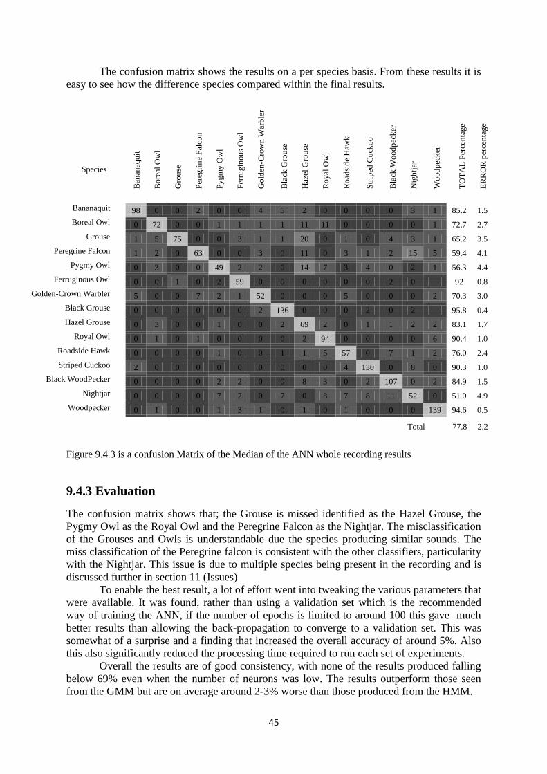
45
The confusion matrix shows the results on a per species basis. From these results it is
easy to see how the difference species compared within the final results.
Species
Ban
anaq
uit
Bo
real
Ow
l
Gro
use
Per
egri
ne
Fal
con
Py
gm
y O
wl
Fer
rug
inou
s O
wl
Go
lden
-Cro
wn
War
ble
r
Bla
ck G
rou
se
Haz
el G
rou
se
Ro
yal
Ow
l
Ro
adsi
de
Haw
k
Str
iped
Cu
cko
o
Bla
ck W
ood
pec
ker
Nig
htj
ar
Wo
od
pec
ker
TO
TA
L P
erce
nta
ge
ER
RO
R p
erce
nta
ge
Bananaquit 98 0 0 2 0 0 4 5 2 0 0 0 0 3 1 85.2 1.5
Boreal Owl 0 72 0 0 1 1 1 1 11 11 0 0 0 0 1 72.7 2.7
Grouse 1 5 75 0 0 3 1 1 20 0 1 0 4 3 1 65.2 3.5
Peregrine Falcon 1 2 0 63 0 0 3 0 11 0 3 1 2 15 5 59.4 4.1
Pygmy Owl 0 3 0 0 49 2 2 0 14 7 3 4 0 2 1 56.3 4.4
Ferruginous Owl 0 0 1 0 2 59 0 0 0 0 0 0 2 0 92 0.8
Golden-Crown Warbler 5 0 0 7 2 1 52 0 0 0 5 0 0 0 2 70.3 3.0
Black Grouse 0 0 0 0 0 0 2 136 0 0 0 2 0 2 95.8 0.4
Hazel Grouse 0 3 0 0 1 0 0 2 69 2 0 1 1 2 2 83.1 1.7
Royal Owl 0 1 0 1 0 0 0 0 2 94 0 0 0 0 6 90.4 1.0
Roadside Hawk 0 0 0 0 1 0 0 1 1 5 57 0 7 1 2 76.0 2.4
Striped Cuckoo 2 0 0 0 0 0 0 0 0 0 4 130 0 8 0 90.3 1.0
Black WoodPecker 0 0 0 0 2 2 0 0 8 3 0 2 107 0 2 84.9 1.5
Nightjar 0 0 0 0 7 2 0 7 0 8 7 8 11 52 0 51.0 4.9
Woodpecker 0 1 0 0 1 3 1 0 1 0 1 0 0 0 139 94.6 0.5
Total 77.8 2.2
Figure 9.4.3 is a confusion Matrix of the Median of the ANN whole recording results
9.4.3 Evaluation
The confusion matrix shows that; the Grouse is missed identified as the Hazel Grouse, the
Pygmy Owl as the Royal Owl and the Peregrine Falcon as the Nightjar. The misclassification
of the Grouses and Owls is understandable due the species producing similar sounds. The
miss classification of the Peregrine falcon is consistent with the other classifiers, particularity
with the Nightjar. This issue is due to multiple species being present in the recording and is
discussed further in section 11 (Issues)
To enable the best result, a lot of effort went into tweaking the various parameters that
were available. It was found, rather than using a validation set which is the recommended
way of training the ANN, if the number of epochs is limited to around 100 this gave much
better results than allowing the back-propagation to converge to a validation set. This was
somewhat of a surprise and a finding that increased the overall accuracy of around 5%. Also
this also significantly reduced the processing time required to run each set of experiments.
Overall the results are of good consistency, with none of the results produced falling
below 69% even when the number of neurons was low. The results outperform those seen
from the GMM but are on average around 2-3% worse than those produced from the HMM.
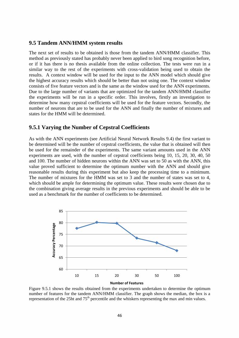
46
9.5 Tandem ANN/HMM system results
The next set of results to be obtained is those from the tandem ANN/HMM classifier. This
method as previously stated has probably never been applied to bird song recognition before,
or if it has there is no thesis available from the online collection. The tests were run in a
similar way to the rest of the experiments with cross-validation being used to obtain the
results. A context window will be used for the input to the ANN model which should give
the highest accuracy results which should be better than not using one. The context window
consists of five feature vectors and is the same as the window used for the ANN experiments.
Due to the large number of variants that are optimized for the tandem ANN/HMM classifier
the experiments will be run in a specific order. This involves, firstly an investigation to
determine how many cepstral coefficients will be used for the feature vectors. Secondly, the
number of neurons that are to be used for the ANN and finally the number of mixtures and
states for the HMM will be determined.
9.5.1 Varying the Number of Cepstral Coefficients
As with the ANN experiments (see Artificial Neural Network Results 9.4) the first variant to
be determined will be the number of cepstral coefficients, the value that is obtained will then
be used for the remainder of the experiments. The same variant amounts used in the ANN
experiments are used, with the number of cepstral coefficients being 10, 15, 20, 30, 40, 50
and 100. The number of hidden neurons within the ANN was set to 50 as with the ANN, this
value proved sufficient to determine the optimum number with the ANN and should give
reasonable results during this experiment but also keep the processing time to a minimum.
The number of mixtures for the HMM was set to 3 and the number of states was set to 4,
which should be ample for determining the optimum value. These results were chosen due to
the combination giving average results in the previous experiments and should be able to be
used as a benchmark for the number of coefficients to be determined.
Figure 9.5.1 shows the results obtained from the experiments undertaken to determine the optimum
number of features for the tandem ANN/HMM classifier. The graph shows the median, the box is a
representation of the 25ht and 75th percentile and the whiskers representing the max and min values.
60
65
70
75
80
85
10 15 20 30 50 100
Acc
ura
cy P
erc
en
tage
Number of Features
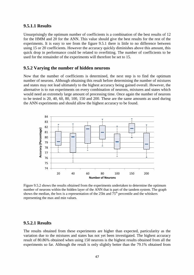
47
9.5.1.1 Results
Unsurprisingly the optimum number of coefficients is a combination of the best results of 12
for the HMM and 20 for the ANN. This value should give the best results for the rest of the
experiments. It is easy to see from the figure 9.5.1 there is little to no difference between
using 15 or 20 coefficients. However the accuracy quickly diminishes above this amount, this
quick drop in performance could be related to overfitting. The number of coefficients to be
used for the remainder of the experiments will therefore be set to 15.
9.5.2 Varying the number of hidden neurons
Now that the number of coefficients is determined, the next step is to find the optimum
number of neurons. Although obtaining this result before determining the number of mixtures
and states may not lead ultimately to the highest accuracy being gained overall. However, the
alternative is to run experiments on every combination of neurons, mixtures and states which
would need an extremely large amount of processing time. Once again the number of neurons
to be tested is 20, 40, 60, 80, 100, 150 and 200. These are the same amounts as used during
the ANN experiments and should allow the highest accuracy to be found.
Figure 9.5.2 shows the results obtained from the experiments undertaken to determine the optimum
number of neurons within the hidden layer of the ANN that is part of the tandem system. The graph
shows the median, the box is a representation of the 25ht and 75th percentile and the whiskers
representing the max and min values.
9.5.2.1 Results
The results obtained from these experiments are higher than expected, particularity as the
variation due to the mixtures and states has not yet been investigated. The highest accuracy
result of 80.86% obtained when using 150 neurons is the highest results obtained from all the
experiments so far. Although the result is only slightly better than the 79.1% obtained from
74
75
76
77
78
79
80
81
82
83
84
20 40 60 80 100 150 200
Acc
ura
cy (
Pe
rce
nta
ge)
Number of Neurons
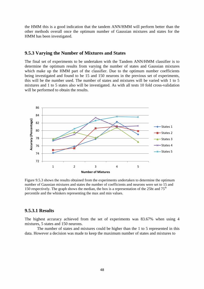
48
the HMM this is a good indication that the tandem ANN/HMM will perform better than the
other methods overall once the optimum number of Gaussian mixtures and states for the
HMM has been investigated.
9.5.3 Varying the Number of Mixtures and States
The final set of experiments to be undertaken with the Tandem ANN/HMM classifier is to
determine the optimum results from varying the number of states and Gaussian mixtures
which make up the HMM part of the classifier. Due to the optimum number coefficients
being investigated and found to be 15 and 150 neurons in the previous set of experiments,
this will be the number used. The number of states and mixtures will be varied with 1 to 5
mixtures and 1 to 5 states also will be investigated. As with all tests 10 fold cross-validation
will be performed to obtain the results.
Figure 9.5.3 shows the results obtained from the experiments undertaken to determine the optimum
number of Gaussian mixtures and states the number of coefficients and neurons were set to 15 and
150 respectively. The graph shows the median, the box is a representation of the 25ht and 75th
percentile and the whiskers representing the max and min values.
9.5.3.1 Results
The highest accuracy achieved from the set of experiments was 83.67% when using 4
mixtures, 5 states and 150 neurons.
The number of states and mixtures could be higher than the 1 to 5 represented in this
data. However a decision was made to keep the maximum number of states and mixtures to
72
74
76
78
80
82
84
86
1 2 3 4 5
Acc
ura
cy (
Pe
rce
nta
ge)
Number of Mixtures
States 1
States 2
States 3
States 4
States 5
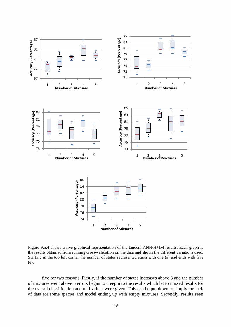
49
Figure 9.5.4 shows a five graphical representation of the tandem ANN/HMM results. Each graph is
the results obtained from running cross-validation on the data and shows the different variations used.
Starting in the top left corner the number of states represented starts with one (a) and ends with five
(e).
five for two reasons. Firstly, if the number of states increases above 3 and the number
of mixtures went above 5 errors began to creep into the results which let to missed results for
the overall classification and null values were given. This can be put down to simply the lack
of data for some species and model ending up with empty mixtures. Secondly, results seen
67
72
77
82
87
1 2 3 4 5
Acc
ura
cy (
Pe
rce
nta
ge)
Number of Mixtures
71
73
75
77
79
81
83
85
1 2 3 4 5
Acc
ura
cy (
Pe
rce
nta
ge)
Number of Mixtures
73
75
77
79
81
83
1 2 3 4 5
Acc
ura
cy (
Pe
rce
nta
ge)
Number of Mixtures
73
75
77
79
81
83
85
1 2 3 4 5
Acc
ura
cy (
Pe
rce
nta
ge)
Number of Mixtures
74
76
78
80
82
84
86
1 2 3 4 5
Acc
ura
cy (
Pe
rce
nta
ge)
Number of Mixtures
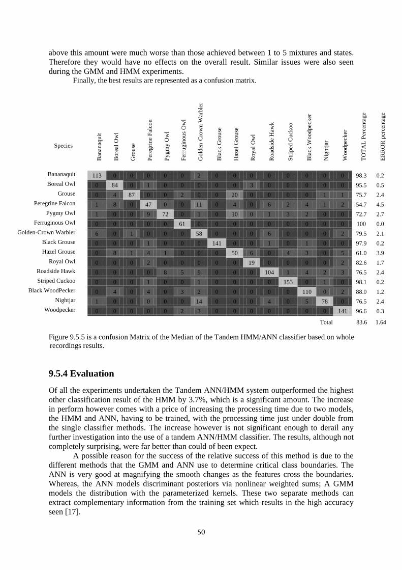
50
above this amount were much worse than those achieved between 1 to 5 mixtures and states.
Therefore they would have no effects on the overall result. Similar issues were also seen
during the GMM and HMM experiments. Finally, the best results are represented as a confusion matrix.
9.5.4 Evaluation
Of all the experiments undertaken the Tandem ANN/HMM system outperformed the highest
other classification result of the HMM by 3.7%, which is a significant amount. The increase
in perform however comes with a price of increasing the processing time due to two models,
the HMM and ANN, having to be trained, with the processing time just under double from
the single classifier methods. The increase however is not significant enough to derail any
further investigation into the use of a tandem ANN/HMM classifier. The results, although not
completely surprising, were far better than could of been expect.
A possible reason for the success of the relative success of this method is due to the
different methods that the GMM and ANN use to determine critical class boundaries. The
ANN is very good at magnifying the smooth changes as the features cross the boundaries.
Whereas, the ANN models discriminant posteriors via nonlinear weighted sums; A GMM
models the distribution with the parameterized kernels. These two separate methods can
extract complementary information from the training set which results in the high accuracy
seen [17].
Species
Ban
anaq
uit
Bo
real
Ow
l
Gro
use
Per
egri
ne
Fal
con
Py
gm
y O
wl
Fer
rug
inou
s O
wl
Go
lden
-Cro
wn
War
ble
r
Bla
ck G
rou
se
Haz
el G
rou
se
Ro
yal
Ow
l
Ro
adsi
de
Haw
k
Str
iped
Cu
cko
o
Bla
ck W
ood
pec
ker
Nig
htj
ar
Wo
od
pec
ker
TO
TA
L P
erce
nta
ge
ER
RO
R p
erce
nta
ge
Bananaquit 113 0 0 0 0 0 2 0 0 0 0 0 0 0 0 98.3 0.2
Boreal Owl 0 84 0 1 0 0 0 0 0 3 0 0 0 0 0 95.5 0.5
Grouse 0 4 87 0 0 2 0 0 20 0 0 0 0 1 1 75.7 2.4
Peregrine Falcon 1 8 0 47 0 0 11 0 4 0 6 2 4 1 2 54.7 4.5
Pygmy Owl 1 0 0 9 72 0 1 0 10 0 1 3 2 0 0 72.7 2.7
Ferruginous Owl 0 0 0 0 0 61 0 0 0 0 0 0 0 0 0 100 0.0
Golden-Crown Warbler 6 0 1 0 0 0 58 0 0 0 6 0 0 0 2 79.5 2.1
Black Grouse 0 0 0 1 0 0 0 141 0 0 1 0 1 0 0 97.9 0.2
Hazel Grouse 0 8 1 4 1 0 0 0 50 6 0 4 3 0 5 61.0 3.9
Royal Owl 0 0 0 2 0 0 0 0 0 19 0 0 0 0 2 82.6 1.7
Roadside Hawk 0 0 0 0 8 5 9 0 0 0 104 1 4 2 3 76.5 2.4
Striped Cuckoo 0 0 0 1 0 0 1 0 0 0 0 153 0 1 0 98.1 0.2
Black WoodPecker 0 4 0 4 0 3 2 0 0 0 0 0 110 0 2 88.0 1.2
Nightjar 1 0 0 0 0 0 14 0 0 0 4 0 5 78 0 76.5 2.4
Woodpecker 0 0 0 0 0 2 3 0 0 0 0 0 0 0 141 96.6 0.3
Total 83.6 1.64
Figure 9.5.5 is a confusion Matrix of the Median of the Tandem HMM/ANN classifier based on whole
recordings results.
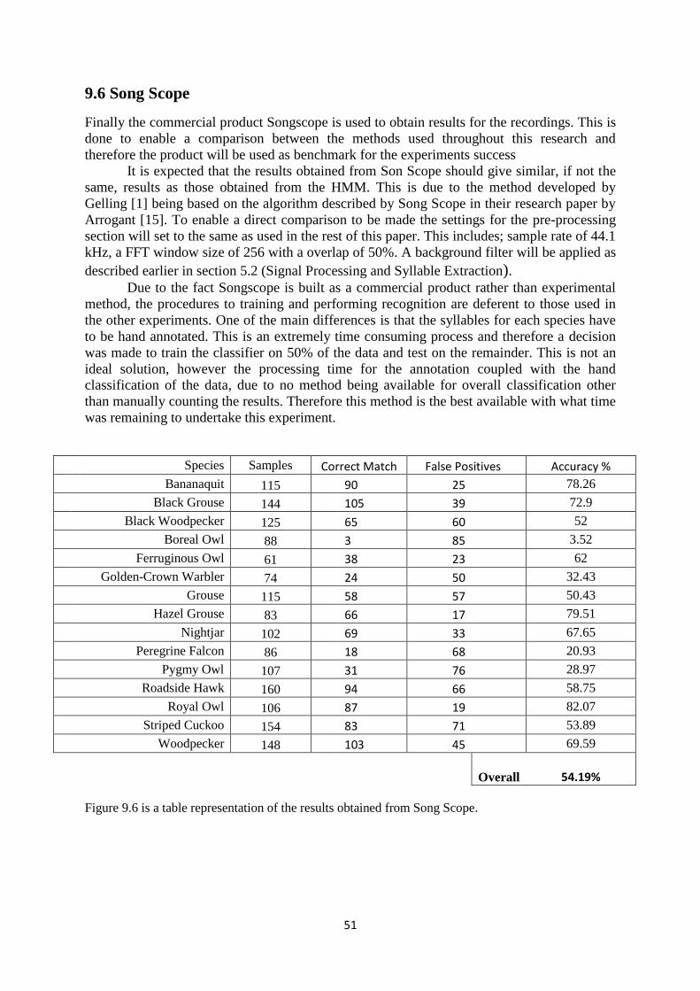
51
9.6 Song Scope
Finally the commercial product Songscope is used to obtain results for the recordings. This is
done to enable a comparison between the methods used throughout this research and
therefore the product will be used as benchmark for the experiments success
It is expected that the results obtained from Son Scope should give similar, if not the
same, results as those obtained from the HMM. This is due to the method developed by
Gelling [1] being based on the algorithm described by Song Scope in their research paper by
Arrogant [15]. To enable a direct comparison to be made the settings for the pre-processing
section will set to the same as used in the rest of this paper. This includes; sample rate of 44.1
kHz, a FFT window size of 256 with a overlap of 50%. A background filter will be applied as
described earlier in section 5.2 (Signal Processing and Syllable Extraction).
Due to the fact Songscope is built as a commercial product rather than experimental
method, the procedures to training and performing recognition are deferent to those used in
the other experiments. One of the main differences is that the syllables for each species have
to be hand annotated. This is an extremely time consuming process and therefore a decision
was made to train the classifier on 50% of the data and test on the remainder. This is not an
ideal solution, however the processing time for the annotation coupled with the hand
classification of the data, due to no method being available for overall classification other
than manually counting the results. Therefore this method is the best available with what time
was remaining to undertake this experiment.
Species Samples Correct Match False Positives Accuracy %
Bananaquit 115 90 25 78.26
Black Grouse 144 105 39 72.9
Black Woodpecker 125 65 60 52
Boreal Owl 88 3 85 3.52
Ferruginous Owl 61 38 23 62
Golden-Crown Warbler 74 24 50 32.43
Grouse 115 58 57 50.43
Hazel Grouse 83 66 17 79.51
Nightjar 102 69 33 67.65
Peregrine Falcon 86 18 68 20.93
Pygmy Owl 107 31 76 28.97
Roadside Hawk 160 94 66 58.75
Royal Owl 106 87 19 82.07
Striped Cuckoo 154 83 71 53.89
Woodpecker 148 103 45 69.59
Overall 54.19%
Figure 9.6 is a table representation of the results obtained from Song Scope.
52
9.6.1 Results
The results for the Songscope experiments overall was 54.2%, which is much lower than
expected. The results are significantly lower than the 79.1% produced by the HMM which
was constructed by Gelling [1], which is quite surprising. This result were expected to be
within at least 5-10% of that seen from the HMM results. The results, however, are consistent
with those obtained from the software by Brown et al [4] of 52.4%.
To understand why the software produced such a low accuracy score, a couple of
reasons are queried. Firstly, the recognizer was only trained on 50% of the data. Early
experiments with the HMM method showed that there is quite a considerable gain to be
achieved by training the model on 90% of the data rather than the 50% used, however the
drop in perform for the HMM was never as low as the result seen by Song Scope.
Secondly, although the HMM classifier produced by Gelling [1] was based on the
algorithm discussed in the Song Scope paper, the methods might of varied slightly. For
instance, the method used by Gelling to locate the syllables is automated and uses the power
spectrum energy to determine the location of the syllable. However, Song Scope uses hand
labelling. Maybe this leads to the HMM method only selecting the best syllables. Also, the
variation in the toolkit being used may lead to different in results. However this seems
unlikely.
Undertaking the research into using Song Scope had to limited due to time
constraints, this was due to the software differing from all the other techniques and the other
experiments taking longer than expected. Although saying this, several days were allocated to
the work with Song Scope. However as previously stated the results that are obtained are
geared towards bird recognitions rather than overall recording accuracy results and a great
deal of effort had to be undertaken to obtain the results so that an overall recogniser average
could be gained.
Although the reasons given here go some way to explaining the result obtained, it is
still hard to understand why the result obtained was so much lower than those obtained by the
hand coded HMM. With the pre-processing section of the algorithms being similar, if not the
same, it is difficult to understand how the software could perform relatively so poorly. It is
however very difficult to draw a conclusion from this result, with one of the results being as
low as 3% it is difficult to justify.
10. Overall Results Review
A final look at the results shows a comparison between the most accurate results that were
obtained from each classifier results. The highest accuracy recorded from each of the results
is depicted in the result chart in figure 10. The chart gives a good representation of the
relevant accuracy for the different ASR methods and applying them to bird song recognition.
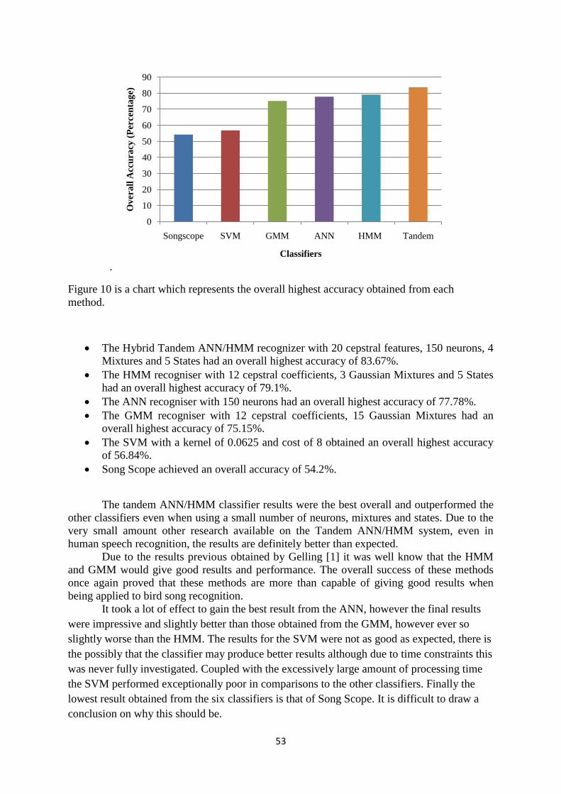
53
.
Figure 10 is a chart which represents the overall highest accuracy obtained from each
method.
The Hybrid Tandem ANN/HMM recognizer with 20 cepstral features, 150 neurons, 4
Mixtures and 5 States had an overall highest accuracy of 83.67%.
The HMM recogniser with 12 cepstral coefficients, 3 Gaussian Mixtures and 5 States
had an overall highest accuracy of 79.1%.
The ANN recogniser with 150 neurons had an overall highest accuracy of 77.78%.
The GMM recogniser with 12 cepstral coefficients, 15 Gaussian Mixtures had an
overall highest accuracy of 75.15%.
The SVM with a kernel of 0.0625 and cost of 8 obtained an overall highest accuracy
of 56.84%.
Song Scope achieved an overall accuracy of 54.2%.
The tandem ANN/HMM classifier results were the best overall and outperformed the
other classifiers even when using a small number of neurons, mixtures and states. Due to the
very small amount other research available on the Tandem ANN/HMM system, even in
human speech recognition, the results are definitely better than expected.
Due to the results previous obtained by Gelling [1] it was well know that the HMM
and GMM would give good results and performance. The overall success of these methods
once again proved that these methods are more than capable of giving good results when
being applied to bird song recognition.
It took a lot of effect to gain the best result from the ANN, however the final results
were impressive and slightly better than those obtained from the GMM, however ever so
slightly worse than the HMM. The results for the SVM were not as good as expected, there is
the possibly that the classifier may produce better results although due to time constraints this
was never fully investigated. Coupled with the excessively large amount of processing time
the SVM performed exceptionally poor in comparisons to the other classifiers. Finally the
lowest result obtained from the six classifiers is that of Song Scope. It is difficult to draw a
conclusion on why this should be.
0
10
20
30
40
50
60
70
80
90
Songscope SVM GMM ANN HMM Tandem
Ov
era
ll A
ccu
racy
(P
erce
nta
ge)
Classifiers
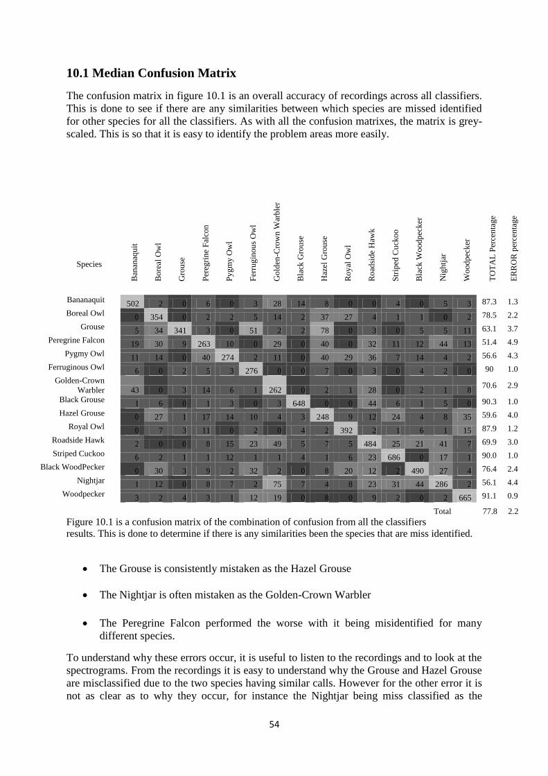
54
10.1 Median Confusion Matrix
The confusion matrix in figure 10.1 is an overall accuracy of recordings across all classifiers.
This is done to see if there are any similarities between which species are missed identified
for other species for all the classifiers. As with all the confusion matrixes, the matrix is grey-
scaled. This is so that it is easy to identify the problem areas more easily.
Figure 10.1 is a confusion matrix of the combination of confusion from all the classifiers
results. This is done to determine if there is any similarities been the species that are miss identified.
The Grouse is consistently mistaken as the Hazel Grouse
The Nightjar is often mistaken as the Golden-Crown Warbler
The Peregrine Falcon performed the worse with it being misidentified for many
different species.
To understand why these errors occur, it is useful to listen to the recordings and to look at the
spectrograms. From the recordings it is easy to understand why the Grouse and Hazel Grouse
are misclassified due to the two species having similar calls. However for the other error it is
not as clear as to why they occur, for instance the Nightjar being miss classified as the
Species
Ban
anaq
uit
Bo
real
Ow
l
Gro
use
Per
egri
ne
Fal
con
Py
gm
y O
wl
Fer
rug
inou
s O
wl
Go
lden
-Cro
wn
War
ble
r
Bla
ck G
rou
se
Haz
el G
rou
se
Ro
yal
Ow
l
Ro
adsi
de
Haw
k
Str
iped
Cu
cko
o
Bla
ck W
ood
pec
ker
Nig
htj
ar
Wo
od
pec
ker
TO
TA
L P
erce
nta
ge
ER
RO
R p
erce
nta
ge
Bananaquit
502 2 0 6 0 3 28 14 8 0 0 4 0 5 3 87.3 1.3
Boreal Owl
0 354 0 2 2 5 14 2 37 27 4 1 1 0 2 78.5 2.2
Grouse
5 34 341 3 0 51 2 2 78 0 3 0 5 5 11 63.1 3.7
Peregrine Falcon
19 30 9 263 10 0 29 0 40 0 32 11 12 44 13 51.4 4.9
Pygmy Owl
11 14 0 40 274 2 11 0 40 29 36 7 14 4 2 56.6 4.3
Ferruginous Owl
6 0 2 5 3 276 0 0 7 0 3 0 4 2 0 90 1.0
Golden-Crown
Warbler
43 0 3 14 6 1 262 0 2 1 28 0 2 1 8 70.6 2.9
Black Grouse
1 6 0 1 3 0 3 648 0 0 44 6 1 5 0 90.3 1.0
Hazel Grouse
0 27 1 17 14 10 4 3 248 9 12 24 4 8 35 59.6 4.0
Royal Owl
0 7 3 11 0 2 0 4 2 392 2 1 6 1 15 87.9 1.2
Roadside Hawk
2 0 0 8 15 23 49 5 7 5 484 25 21 41 7 69.9 3.0
Striped Cuckoo
6 2 1 1 12 1 1 4 1 6 23 686 0 17 1 90.0 1.0
Black WoodPecker
0 30 3 9 2 32 2 0 8 20 12 2 490 27 4 76.4 2.4
Nightjar
1 12 0 8 7 2 75 7 4 8 23 31 44 286 2 56.1 4.4
Woodpecker
3 2 4 3 1 12 19 0 8 0 9 2 0 2 665 91.1 0.9
Total 77.8 2.2
55
Golden-Crown Warbler due to their calls not being similar. This could be due to the two calls
having similar frequency ranges or the overall phasing being similar, although it is still clear
for a human listener that they are different. The problem may lie, also that of the peregrine
falcon, with the amount of background noise within these recordings. These two species in
particular had a very high number of other species present and this maybe the cause of much
of the problems. The Grouse and Nightjar have particularity long recordings compared to
some of the other species that performed better. Also, the calls in general for these two birds
are generally a long distance away from the recording device and maybe difficult for the
recognisers to detect due to the volume of the vocalisation within the recording.
11. Objectives
The purpose of this paper was to determine the relative success of 5 different methods of
automated speech recognition and applying them to bird song vocalisation detection and
compare them to the commercial produce Songscope.
The first objective was to construct the different classifiers. Although this was
relatively straightforward due to the toolkits, the different methods implemented by the
toolkits in regards to data handling did present somewhat of a problem. With the pre-
processing already been constructed by Gelling [1] the data, once the pre-processing was
complete, had to be manipulated into different data structures to be used by the different
methods. This manipulation could be time consuming and could result in large amounts of
processing time, however, a solution to this problem which eradicated much of this overhead.
Once this was overcome the methods were relatively easy to implement, although the tandem
HMM/ANN classifier was by far the most difficult of the three constructed methods (with the
GMM and HMM previously being constructed by Gelling)
To enable a fair comparison, although not in all cases possible, the test situations,
other than the classifiers internal variations, remained constant. This involved selecting 15
species from a large corpus of data and constantly using the same data throughout the
experiments. The features extraction method was consistent and was similar to the methods
used internally by Songscope, which resulted in cepstral coefficients similar to MFCCs being
produced. To enable the selection of the syllables for all methods the iterative algorithm
based on the one employed by Fagerlund [5] was implemented. Although this option of
automatic syllable selection is not available as part of the Songscope therefore the syllables
had to be hand selected for the software which was extremely time consuming.
All experiments were conducted by using the syllables obtained during the
syllable selection process and training the classifiers on these features. A further set of data
was obtained from between the syllable and was used as background noise and which the
classifiers were also trained on. By doing this it allowed recognition to be attempted on whole
recording, which should have produced results that are similar to those that the classifiers
would produce in a real world situation. Once the recognition had taken place the “silent”
frames were negated and recognition was determined on the remaining frames. All
experiments were conducted using 10 fold cross-validation apart from the SVM and
Songscope due to emigrating circumstances as discussed earlier. Finally for species
recognition, either the Viterbi algorithm or frame-by-by analysis was used depending on
whether the temporal information was taken into account by the classifier, with all classifiers
results being represented in confusion matrix form.
Overall the objective to enable comparison between the different classifiers seems to
have been met. With the obvious exception being Son Scope due to the results being worse
than the results obtained from the HMM produced by Gelling [1]. This maybe can be put
56
down to the time consuming nature of the hand annotating of the data and only 50% of the
data being used for training. This seems to had a detrimental effect on the overall accuracy of
the software, however as previously stated when this method is used with Gelling‟s [1] HMM
algorithm the results are still much higher than the results produced by Song Scope.
Other than this the objectives for all experiments seems to have been met and the best
results for each classifier for the data should of been found, possibly with the exception of the
SVM.
12. Issues
The main issues that were experience during the research was relating to the data and also the
amount of processing time required to conduct the experiments. The main issues with the
data was that most of the Italian recording were hand selected and consisted of very long
recordings which spanned a birds repetitive call cycle. The problem being that there may
have been 5-10 calls from the bird under investigation but more calls from other species.
Which made it extremely difficult to decipher the different birds calls within the recording,
even my a human listener.. It was particular difficult to determine the species considering the
birds description where all in Italian. Once the information of the species was gained it
became apparent that most of the recording were of birds of prey or other species that are
endangered. This in itself produces problems, due to the nature of such species they are not
numerous in number, therefore the number of recordings available of the birds is low which
lows the quality of the recordings in respect the number of vocalisations available of the
species. This had an effect in respect to many of the recordings prominently contained
common song birds in the foreground with the research birds call being faintly heard in the
background. The effect of this was during training of the classifiers the more prominent
foreground multitude of species (including calls from species that were being used during this
research) were being trained. This resulted in some species with a large amount of other bird
interference resulting in a large amount of the borderline discussions being returned as false
positives and the overall results being poor. A decision was therefore made to reduce the
recording length to minimize the amount of interference from other species at the beginning
and end of the period of vocalisation. Although interference from other species was still
present, the orientation of the recordings was more focused on the expected species. This
seemed to have the desired effect and the large amount of false positive that were being
obtained was significantly reduced. The consequence of this was many pain staking hours
removing large amounts of effective background noise from the recordings and large periods
of saturation from before and after the vocalisations. However the efforts produced
noteworthy results.
Another issue was to do with the amount of processing time to train the classifiers on
a large amount of data, which lead to large amount of data having to be processed each
experiment. The issue was not so vast when working with the GMM and HMM. The ANN
and SVM in particular the training time could well exceed several hours. To run the SVM
with such a large amount of data took around a week to complete two runs and the results
after this immense amount of time were still poor. Great effect was made to attempt to reduce
the processing time relating to the ANN which was achieved by tweaking code until good
results were seen and low processing times. The Tandem HMM/ANN also suffered due to the
need to train two different methods in each of the experiments. However, once a successful
method of reducing the training for ANN this also had an effect on the tandem classifier.
57
13. Discussion
To determine the relative success of the research the results achieved during the experiments
need to compared and analysed to previous work undertaken and which was reviewed in the
literature review (see section 3). To begin with, there is an easy comparison to be made
between the results obtained in this research and the results obtained by Gelling [1]. This is
due to the same GMM and HMM methods being used in both research. The results from the
experiments conducted in this research have shown a reduction in accuracy by around 3%
and 5% respectively. The reduction, although expected, can be put down to two facts. Firstly
the amount of data increasing from 5 to 15 species increased the probability of miss
classification which resulted in more false positive results. Secondly, the Italian data was
much rawer data than the handpicked Brown et al [4] data in the sense that the data contained
multiple calls (not always of the expected species) and were on average of a longer length.
However this said, both classifiers performed comparatively well and the results from both
methods were still promising.
Compared to the other departmental work carried out by Brown et al [4], the results
obtained for the GMM and SVM of 65.5% and 40.6% are lower than the results found in this
research. The results for the GMM are lower than even the mean average results obtained
from using one mixture, but only slightly by 2%. A possible explanation for the results
obtained during this research being higher is due to the different methods used to create the
feature. In the research carried out by Brown et al [4] there seems to be no attempt to remove
the background noise from the recordings. The data was processed by taking a FFT of the
windowed data, once this has been done a DCT is taken straight after the FFT, Also, there is
no attempt made to transform the data into a log-frequency domain or normalise it.
Additionally to this, the full frequency range is used instead of limiting the frequency to that
which contained the bird‟s vocalisation. This is probably why the performance in the research
by Brown et al [4] is seemingly worse than the results obtained here.
The research conducted by McIlraith et al [18] produced higher results than those
seen during this research for the ANN classifier, which were slightly higher at 80 to 85%.
However the number of samples and species used in their experiments was much lower than
the amount used in this research. A hint of the duration between each syllable was also given
to the classifier and therefore aided the overall classification results. Due to the low number
of samples being used it is difficult to draw a comparison from the two separate results.
The next paper that was reviewed was the research conducted by Cia et al [12]. This
research is similar to the methods used in this paper in respect to the use of a five frame
context window, RPROP for the training algorithm, a multi-layer perception neural network
was used for classification and 14 species were used. The papers difference due to the
methods used to extract the features (MFCCs) and the use a time delay input to the MLP. The
results obtained by Cia et al were much better than the results seen in all experiments in this
research, the results 86.6% is even better than the results seen by the Tandem HMM/ANN
system. A possibly reason for this could be the use of a delay on the input to the neural
network, however preliminary research that was carried out concluded that applying such a
method only very marginally, if at all, increased the results. It did however increase process
time massively and lead to many of the experiments returning an out of memory error, even
with 8GB ram installed. However more importantly the fifteen species used during the Cia et
al [12] experiments were all taken from a CD, this high quality recording is probably the
difference that is seen between the two experiments results. Also the paper doesn‟t confirm
how many features are used during the experiments.
In another paper written by Ross [16] the comparative success of an ANN, SVM and
KDE are explored. Similar methods used to produce the ANN and SVM using Matlab, neural
58
network toolkit and LIBSVM were used. The results for the ANN of 83% and 76% for the
SVM are higher than the results seen in the experiments conducted here. This can again
possibly be put down to the audio being taken from a CD, with will have little to no inference
from other species or saturation. Also, any recordings with high level of background noise
were omitted from the study. Therefore no attempt was made during pre-process to remove
the background noise. The recordings were simply converted to the cepstral domain and the
first twenty features were extracted. The results found in this research and found by Ross
both imply that the ANN is better at matching vocalisations than the SVM.
The work undertaken by Fagerlund [6] was to investigate the use of the SVM
algorithm and applying to bird recording recognition. During Fagerlund‟s [6] research two
different sets of species were investigated and the different effect of MFCC, MFCC delta,
MFCC delta-delta and a mixture model (delta and delta-delta coefficients) were investigated.
The results obtained in the experiments were near perfect results of 96-98%. These results are
far higher than the results obtained during this research. A reason for this is that the syllable
were manually segmented, all background noise was removed and other species interference.
Also a much smaller number of species, six, were used compared to experiments conducted
during this research. Also the aim of the paper was not to determine the best results for
classification but the best combination of coefficients.
The final paper is produced by Songscope and which reviewed the performance of
their own software. The application was tested on 52 species with around 54 different
vocalisations per species. The training was done on syllables and the recognition performed
on the full recording, similar to the methods used in this paper. The performance of the
classification was 67% on the training data which fell to 37% on the testing data. These
results are lower than the 54.2% obtained from the Songscope experiment that were detailed
here, also the results are much lower than the results from the other classifiers which all
performed better than these results. There are two contributing factors to this. Firstly, the
number of species is much higher that the amount used in this research, therefore the baseline
accuracy estimation is much lower, also the possibility of two species having similar
vocalisations increases.
Secondly, the Songscope research was focusing on how well the product was able to
perform in a real world situation. With many of the recordings containing multiple species
and the overall goal was to keep the false positive rate to a minimum, which effectively
reduces the true positive rate also. This therefore makes it difficult to make a direct
comparison between the two experiments [1].
14. Conclusion
Overall the results obtained seem to be a true representation of the classifiers relative
perform and should be noteworthy result in regards to future research that is conducted within
the field. Possibly for the first time an investigation into five different methods of
classification was performed with their comparable ability to undertake birdsong recognition
compared. The automated speech recognition (ASR) techniques GMM, HMM, ANN, SVM
and a Tandem ANN/HMM system were compared with the commercial software Songscope
being used as final benchmark.
The results showed that by far the worst of the classifiers was the SVM. The results
obtained from this classifier were much lower than the other classifiers and was by far the
longest to train. The results obtained from the GMM, ANN and HMM show that all three
techniques are of similar capability in comparison with the HMM slightly outperforming both
the GMM and ANN. The Tandem HMM/ANN outperformed all the other classifiers by some
59
margin, although had a slight down side in respect to having to train two classifiers resulted
in the training time being slightly longer than the other methods, however this was still within
a manageable time frame. Also, it is quite interesting how the HMM produced in this
research by Gelling [1], on the guidelines of Songscope, was able to outperform Songscope in
the experiments. This could be put down to simple the lack of data that was given to the Song
Scope compared to the handmade HMM or the different toolkits that are used to produce the
two similar methods.
During the investigation into other research undertaken in the field of bird song
recognition it became apparent that it was difficult to compare the relative success of
different classifiers. This was due to the different methods used in each of the papers plus the
ranging quality of the recordings used. The aim of this paper was to produce a standardised
set of results that can be used to identify the relative success of the different methods in
comparisons to each other and to remove the external variations previously mentioned. In this
sense the project has been a success, in regards to producing results with standardised tasks
and a standardised dataset. The obvious success of the tandem ANN/HMM classifier during
this research has shown a method that it seems has never been used previously and shows
potential for any future application use. The research into different methods of automated
speech recognition and applying it to bird song recognition is still a under researched area,
hopefully this work has gone some way as to proving the relative success of different
automated speech recognition methods.
15. Future Directions
Due to much of the data that was used in these experiments being larger birds of prey, many
of the species had one or two distinct calls and not much variation within them. The results
obtained from the research in regard to these species were good, but if more research is to be
undertaken there is a need to obtain recording of species that have a magnitude of calls. This
is so that, an investigation can be made into varying the number of cluster per species and the
possible advantages this may have. This is obviously easier said than done, although much of
the data has been marked with specific species within the Italian data by the Italian
researchers. Much of the data has been divided so that a minute or longer has been identified
as a species. However, these periods usually contain large quantities of different species
vocalisation and it is difficult to detect the species required unless there is previous
experience identifying bird‟s calls. There is also the amount of time it would take to identify
and separate the data into individual calls. Although identifying these issues, there is valuable
research to found in this area.
Additionally to this, research could be undertaken to determine the possibility of
detecting multiple species within a recording. An algorithm could be made that is able to
identify vocalisation by taking a running estimation of the background noise levels, once a
vocalisation is heard the recording is able to recognise the species. This is an algorithm that is
used in Songscope and is able to determine not only if a bird is present but also how many
times a vocalisation is heard. This could be an interesting expansion on the research
conducted in this paper. However, this would require hand selecting good quality recordings
of the species from within the recording that could be used as the training data. Now that the
classifiers are produced and ready to be used, it would be interesting to see how well the
different techniques handle the data and their respective accuracy in a real world situation.
60
5. Bibliography
[1] Douwe Gelling, Bird Song Recognition using GMMs and HMMs.
Unpublished 2010.
[2] Ian Douglas Agranat. Automatically identifying animal species from their vocalisations.
online, 2009. http://www.wildlifeacoustics.com/songscope/aiasftv/aiasftv.pdf.
[3] Ian Douglas Agranat. Automatic detection of cerulean warblers using autonomous
recording units and song scope bioacoustics software. online, 2007.Http://www.wildl-
ifeacoustics.com/songscope/cerulean/AutomaticDetectionOfCeruleanWarblers.pdf.
[4] Mike Brown, Dave Chaston, Adam Cooney, Dharanidhar Maddali, and Thomas Price.
Recognising birds songs - comparative study. unpublished, 2009.
[5] Seppo Fagerlund. Automatic recognition of bird species by their sounds. Master's thesis,
Helsinki University of Technology, 2004.
[6] Seppo Fagerlund. Bird species recognition using support vector machines.
EURASIP J. Appl. Signal Process., 2007(1):64-64, 2007.
[7] Joseph A. Kogan and Daniel Margoliash. Automated recognition of bird song elements
from continuous recordings using dynamic time warping and hidden markov models: A
comparative study. The Journal of the Acoustical Society of America, 103(4):2185-
2196,1998.
[8] Daniel Wolff. Detecting Bird Sounds via Periodic Structures: A Robust Pattern
Recognition Approach to Unsupervised Animal Monitoring. Online. 2008. http://www-
mmdb.iai.uni-bonn.de/download/Diplomarbeiten/Diplomarbeit_Daniel_Wolff.pdf
[9] Allison J. Doupe and Patricia K Kuhl. Birdsong and Human Speech. Annu. Rev.-
Neurosci. 1999. 22:567–631
[10] Chang-Hsing Lee, Yeuan Kuen Lee and Ren-Zhuang Huang. Automated Recognition of
Bird Songs Using Cepstral Coeffients. Journal of Inofrmation Technology and
Applications 2006 (1, 1) 17-23.
[12] Jinhai Cia, Dominic Ee, Paul Roe and Jinglan Zhang. Sensor Network for the monitoring
of Ecosystem: Bird Species Recogntion. 2006 Online http://eprints.qut.edu.au –
/11227/1/11227a.pdf
[13] Prof Leslie Smith. An Introduction to Neural Networks http://www.cs.stir.ac.uk/~lss/-
61
NNIntro/ InvSlides.html. Online 2003. Date accessed 01/12/2011 at 14:15
[14] Christos Stergiou and Dimitrios Siganos http://www.doc.ic.ac.uk/~nd/surprise_96/-
journal/vol4/cs11/report.html/Appendix C - References used throughout the review. Online
Date accessed 01/12/2001 at 14:32
[15] Song Scope, Bioaustics Software Documentation 2007. Online http://www.wildlife –
acoustics.com/scope/SongScope.pdf
[16] Derek J. Ross. Bird Call Recognition With Artificial Neural Networks, Support Vector
Machines and Kernel Density Estimation. University of Manitoba 2006. Online
http://www. antiquark.com/thesis/msc-thesis-derek-ross-v5c.pdf
[17] Hynek Hermansky, Daniel P.W Ellis and Sangita Sharma. Tandem Connectionist feature
extraction for conventional HMM systems. http://troylee.posterous.com/tandem -approach-for-nnhmm.
[18] Alex L. McIlraith and H.C Card. Birdsong recognition with DSP and Neural Networks.
Obtained from Mauro Nicola, PHD student at the University of Sheffield
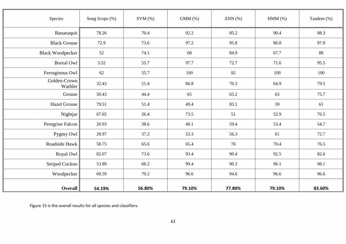
62
Figure 15 is the overall results for all species and classifiers.
Species Song Scope (%) SVM (%) GMM (%) ANN (%) HMM (%) Tandem (%)
Bananaquit 78.26 70.4 92.2 85.2 90.4 98.3
Black Grouse 72.9 73.6 97.2 95.8 86.8 97.9
Black Woodpecker 52 74.1 68 84.9 67.7 88
Boreal Owl 3.52 55.7 97.7 72.7 71.6 95.5
Ferruginous Owl 62 55.7 100 92 100 100
Golden-Crown
Warbler 32.43 51.4 86.8 70.3 64.9 79.5
Grouse 50.43 44.4 65 65.2 63 75.7
Hazel Grouse 79.51 51.4 49.4 83.1 59 61
Nightjar 67.65 26.4 73.5 51 52.9 76.5
Peregrine Falcon 20.93 38.6 49.1 59.4 53.4 54.7
Pygmy Owl 28.97 37.2 53.3 56.3 61 72.7
Roadside Hawk 58.75 65.6 65.4 76 70.4 76.5
Royal Owl 82.07 73.6 93.4 90.4 92.5 82.6
Striped Cuckoo 53.89 66.2 99.4 90.3 96.1 98.1
Woodpecker 69.59 70.2 96.6 94.6 96.6 96.6
Overall 54.19% 56.80% 79.10% 77.80% 79.10% 83.60%
![Chapter 3 Fingerprint Recognition Techniques - …shodhganga.inflibnet.ac.in/bitstream/10603/63746/9/09_chapter 3.pdfChapter 3 Fingerprint Recognition Techniques ... [Wegstein, 1982]](https://img.pdfslide.us/doc/110x75/5ade42a87f8b9a213e8ddfe5/chapter-3-fingerprint-recognition-techniques-3pdfchapter-3-fingerprint-recognition.jpg)