Information Fusion 32 (2016) 80–92

Contents lists available at ScienceDirect

Information Fusion

journal homepage: www.elsevier.com/locate/inffus

An ensemble of patch-based subspaces for makeup-robust

face recognition

Cunjian Chen

a , Antitza Dantcheva

b , Arun Ross c , ∗

a Department of Computer Science and Electrical Engineering, West Virginia University, Morgantown, WV 26506, USA b INRIA, Team STARS, France c Department of Computer Science and Engineering, Michigan State University, East Lansing, MI 48824, USA

a r t i c l e i n f o

Article history:

Available online 10 November 2015

Keywords:

Face recognition

Makeup

Cosmetics

Ensemble learning

Random subspace

a b s t r a c t

Recent research has demonstrated the negative impact of makeup on automated face recognition. In this

work, we introduce a patch-based ensemble learning method, which uses multiple subspaces generated by

sampling patches from before-makeup and after-makeup face images, to address this problem. In the pro-

posed scheme, each face image is tessellated into patches and each patch is represented by a set of feature

descriptors, viz., Local Gradient Gabor Pattern (LGGP), Histogram of Gabor Ordinal Ratio Measures (HGORM)

and Densely Sampled Local Binary Pattern (DS-LBP). Then, an improved Random Subspace Linear Discrimi-

nant Analysis (SRS-LDA) method is used to perform ensemble learning by sampling patches and constructing

multiple common subspaces between before-makeup and after-makeup facial images. Finally, Collaborative-

based and Sparse-based Representation Classifiers are used to compare feature vectors in this subspace and

the resulting scores are combined via the sum-rule. The proposed face matching algorithm is evaluated on

the YMU makeup dataset and is shown to achieve very good results. It outperforms other methods designed

specifically for the makeup problem.

© 2015 Elsevier B.V. All rights reserved.

e

p

m

c

o

1

d

e

a

a

S

w

m

a

t

a

c

1. Introduction

Automated face recognition has been adopted in a broad range of

applications such as personal authentication, video surveillance, im-

age tagging, and human–computer interaction [1] . Automated face

recognition systems recognize an individual by extracting a discrim-

inative set of features from an input face image and comparing this

feature set with a template stored in a database [1] . The recognition

accuracy of these systems has rapidly improved over the past decade

primarily due to the development of robust feature representations

and matching techniques [2–5] , as evidenced by significant reduc-

tion in error rates on several public benchmark databases (e.g., FRGC

[6] , LFW [7] , YTF [8] ). However, a number of challenges still remain

particularly in Heterogeneous Face Recognition where the images to

be matched are fundamentally different, e.g., visible versus thermal

face images or face sketches versus photographs.

More recent research has investigated the problem of matching

faces that have been altered either by plastic surgery [9] or by

the application of facial cosmetics (i.e., makeup). In this work, we

focus on the problem of matching face images before and after the

application of makeup. These images are not acquired in a controlled

∗ Corresponding author.

E-mail address: rossarun@cse.msu.edu , cunjian@msu.edu (A. Ross).

s

http://dx.doi.org/10.1016/j.inffus.2015.09.005

1566-2535/© 2015 Elsevier B.V. All rights reserved.

nvironment, and hence considered as makeup in the wild. This

roblem is especially significant since makeup is a commonly used

odifier of facial appearance. Thus, researchers in biometrics and

ognitive psychology [10] are interested in understanding the effect

f this modifier on face recognition.

.1. Makeup challenge

Recent studies have demonstrated that makeup can significantly

egrade face matching accuracy [11–13] . Makeup is typically used to

nhance or alter the appearance of an individual’s face. It has become

daily necessity for many, as reported in a recent British survey, 1 and

s evidenced by a sale volume of 3.6 Billion in 2011 in the United

tates. 2 The cosmetic industry has developed a number of products,

hich can be broadly categorized as skin, eye or lip makeup. Skin

akeup is utilized to alter skin color and texture, suppress wrinkles,

nd cover blemishes and aging spots. Lip makeup is commonly used

o accentuate the lips (by altering contrast and the perceived shape)

nd to restore moisture. Eye makeup is widely used to increase the

ontrast in the periocular region, change the shape of the eyes, and

1 http://www.superdrug.com/content/ebiz/superdrug/stry/cgq1300799243/

urveyrelease-jp.pdf . 2 https://www.npd.com/wps/portal/npd/us/news/press-releases/pr _ 120301/ .

C. Chen et al. / Information Fusion 32 (2016) 80–92 81

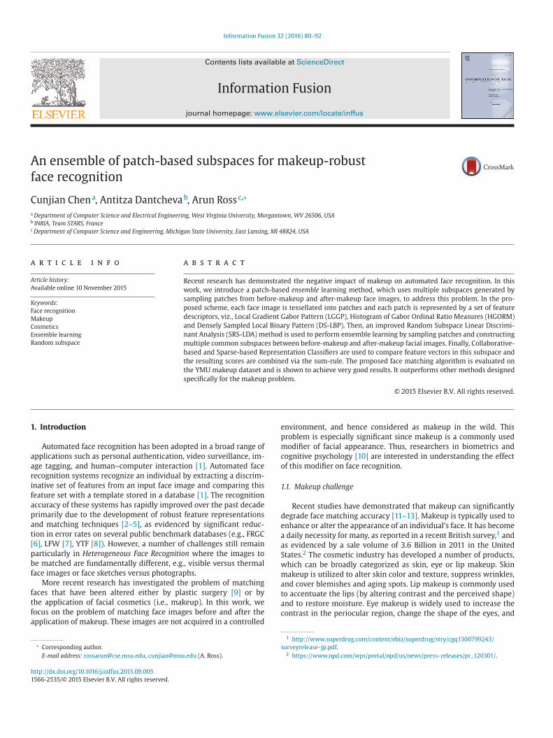
Fig. 1. An example showing how makeup can easily change the overall facial appear-

ance, resulting in possible false non-match errors. Images are obtained from Youtube.

a

o

p

i

t

F

s

r

r

t

o

c

b

r

a

a

c

v

a

c

s

1

c

a

t

[

v

m

p

a

i

(

m

t

a

n

o

a

t

o

b

s

s

l

t

t

s

L

d

t

R

i

s

b

b

e

d

t

t

t

i

a

a

2

r

a

p

b

b

n

a

i

r

m

s

i

b

t

a

b

t

p

s

a

r

s

p

k

s

f

t

m

d

q

o

[

r

f

p

ccentuate the eye-brows [14] . An example demonstrating the impact

f applying makeup can be seen in Fig. 1 .

Makeup poses a challenge to automated face recognition due to its

otential to substantially alter the facial appearance. For example,

t changes the perceived facial shape and appearance, modifies con-

rast levels in the mouth and eye region, and alters skin texture (see

ig. 1 ). Such modifications can lead to large intraclass variations, re-

ulting in false non-matches, where a subject’s face is not successfully

ecognized. Recent work by Dantcheva et al. [11] suggested that the

ecognition accuracy of both commercial and academic face recogni-

ion methods can be reduced by upto 76.21% due to the application

f makeup. 3 It was concluded that non-permanent facial cosmetics

an dramatically change facial appearance, both locally and globally,

y altering color, contrast and texture. Existing face matchers, which

ely on the cues of contrast and texture information for establishing

match, can be impacted by the application of facial makeup. It was

lso observed that the impact due to the application of eye makeup is

onsidered to be more pronounced than lipstick makeup in our pre-

ious work [11] . The combination of eye and lipstick makeups poses

greater challenge than individual ones. Solutions to address this

hallenge are important towards developing robust face recognition

ystems.

.2. Motivation and related work

To date, there is limited scientific literature on addressing the

hallenge of make-up induced changes. Chen et al. [15] presented

n automated makeup detection approach, that was used to adap-

ively modify images prior to performing face recognition. Hu et al.

16] used canonical correlation analysis (CCA) along with a support

ector machine (SVM) classifier to facilitate the matching of before-

akeup and after-makeup images. Guo et al. [12] learned the map-

ing between features extracted from patches in the before- and

fter-makeup images in order to minimize the disparity between the

mages to be matched. The mapping was learned using CCA, rCCA

regularized CCA) and Partial Least Squares (PLS) methods. While

apping-based methods have been shown to be effective, they have

wo main limitations. First, the mapping between before-makeup

nd after-makeup facial images can be complex, spatially variant and

onlinear. Therefore, it is insufficient to learn a single mapping in

rder to describe the complex relationship between before-makeup

nd after-makeup samples [17] . Second, CCA and PLS methods have a

endency to overfit the training data and thus do not generalize well

n unseen subjects [18] .

In order to overcome these problems, we propose to use an ensem-

le learning scheme [19 , 20] to generate multiple common semi-random

ubspaces for before-makeup and after-makeup samples , instead of two

3 http://www.antitza.com/makeup-datasets-benchmark.html .

eparate subspaces. In random subspace methods, a set of multiple

ow-dimensional subspaces are generated by randomly sampling fea-

ure vectors in the original high-dimensional space [21] . It has proven

o be effective in various tasks of face recognition [21–24] . For in-

tance, Wang and Tang [21] proposed the use of Random Subspace

inear Discriminant Analysis (RS-LDA) for face recognition by ran-

omly sampling eigenfaces. Zhu et al. [22] randomly sampled fea-

ures on local image regions to construct a set of base classifiers.

S-LDA method [23,24] was also adapted for matching near-infrared

mages against visible images. The motivation for using a random

ubspace method are as follows [25] : (a) a learning algorithm can

e viewed as searching for the best classifier in a space populated

y different weak classifiers; (b) many weak classifiers are consid-

red to be equally favorable when given a finite amount of training

ata; (c) averaging these individual classifiers can better approximate

he true classifier. Therefore, a random subspace method can be used

o generate multiple common subspaces, where each subspace con-

ains a small portion of discriminative information pertaining to the

dentity. At the same time, by randomly selecting different patches

s the input to each subspace-based classifier, the overfitting issue is

voided [21] .

. Proposed method

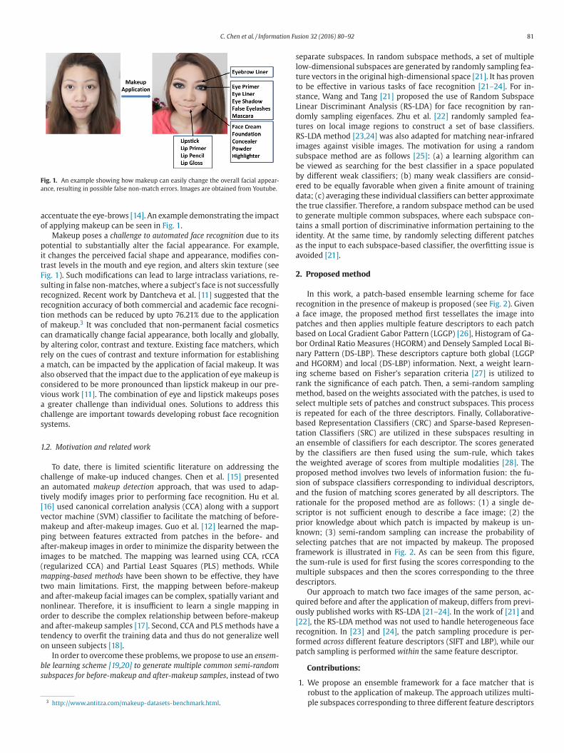
In this work, a patch-based ensemble learning scheme for face

ecognition in the presence of makeup is proposed (see Fig. 2 ). Given

face image, the proposed method first tessellates the image into

atches and then applies multiple feature descriptors to each patch

ased on Local Gradient Gabor Pattern (LGGP) [26] , Histogram of Ga-

or Ordinal Ratio Measures (HGORM) and Densely Sampled Local Bi-

ary Pattern (DS-LBP). These descriptors capture both global (LGGP

nd HGORM) and local (DS-LBP) information. Next, a weight learn-

ng scheme based on Fisher’s separation criteria [27] is utilized to

ank the significance of each patch. Then, a semi-random sampling

ethod, based on the weights associated with the patches, is used to

elect multiple sets of patches and construct subspaces. This process

s repeated for each of the three descriptors. Finally, Collaborative-

ased Representation Classifiers (CRC) and Sparse-based Represen-

ation Classifiers (SRC) are utilized in these subspaces resulting in

n ensemble of classifiers for each descriptor. The scores generated

y the classifiers are then fused using the sum-rule, which takes

he weighted average of scores from multiple modalities [28] . The

roposed method involves two levels of information fusion: the fu-

ion of subspace classifiers corresponding to individual descriptors,

nd the fusion of matching scores generated by all descriptors. The

ationale for the proposed method are as follows: (1) a single de-

criptor is not sufficient enough to describe a face image; (2) the

rior knowledge about which patch is impacted by makeup is un-

nown; (3) semi-random sampling can increase the probability of

electing patches that are not impacted by makeup. The proposed

ramework is illustrated in Fig. 2 . As can be seen from this figure,

he sum-rule is used for first fusing the scores corresponding to the

ultiple subspaces and then the scores corresponding to the three

escriptors.

Our approach to match two face images of the same person, ac-

uired before and after the application of makeup, differs from previ-

usly published works with RS-LDA [21–24] . In the work of [21] and

22] , the RS-LDA method was not used to handle heterogeneous face

ecognition. In [23] and [24] , the patch sampling procedure is per-

ormed across different feature descriptors (SIFT and LBP), while our

atch sampling is performed within the same feature descriptor.

Contributions:

1. We propose an ensemble framework for a face matcher that is

robust to the application of makeup. The approach utilizes multi-

ple subspaces corresponding to three different f eature descriptors

82 C. Chen et al. / Information Fusion 32 (2016) 80–92

Fig. 2. Proposed framework for matching after-makeup images with before-makeup images. During the training phase, for each feature descriptor, a pool of patches is extracted,

followed by weight learning, patch sampling and random subspace construction. In the testing phase, patches from an input image are projected onto the learned random subspace.

A combination of SRC and CRC classifiers are used to compare feature vectors in these subspaces and generate a match score. This process is repeated for each descriptor and the

matching scores corresponding to individual feature descriptors are fused to generate the final similarity score.

r

t

c

i

a

A

a

θ

b

h

e

f

i

t

s

t

t

m

m

G

u

b

s

f

v

t

a

a

d

and multiple image patches. A combination of sparse and collab-

orative classifiers is used in these subspaces.

2. We propose a sampling scheme, which utilizes weight informa-

tion from each patch to guide patch selection, instead of pure ran-

dom sampling.

3. Feature descriptors

The design of effective face image descriptors is considered to

be crucial in face recognition. In this work, the patches in each face

image are represented using LGGP, HGORM and DS-LBP descriptors.

Compared to Dense HOG and Dense LBP used in [23] , LGGP and

HGORM are derived from Gabor-filtered images and have demon-

strated to be more discriminative based on empirical investigation

[26] . Let I ∈ R

128 ×128 denote a face image that is either a before-

makeup sample or an after-makeup sample, and let f denote a fea-

ture extractor. Moreover, z is a generic pixel position, x c is the center

of the rectangle used for coding, which is shifted both horizontally

and vertically along the image. γ c represents the intensity value in

x c . We now describe the three basic feature descriptors used in the

framework.

Gabor filters : A Gabor filter can be mathematically defined as fol-

lows [27] :

ϕ μ,υ(z) =

|| k μ,υ || 2 σ 2

e −|| k μ,υ || 2 || z|| 2

2 σ2 [ e ik μ,υ z − e −σ2

2 ] , (1)

where μ and υ denote the orientation and scale of the Gabor filters,

respectively. z denotes the pixel position and ‖ · ‖ denotes the norm

operator [27] . σ is a constant, which has a default value of 2 π . The

wave vector k μ,υ is given by k μ,υ = k υe iφμ, where k υ = k max /s υ

and φμ = πμ/ 8 . Here, k max is the maximum frequency and s is the

spacing factor between kernels in the frequency domain. The Gabor

esponse of an image is obtained by performing the convolution of

he input image with Gabor kernels: G μ,υ(z) = I(z) ∗ ϕ μ,υ(z). The

omplex Gabor response has two parts: the real part � μ,υ(z) and the

maginary part � μ,υ(z). Accordingly, the Gabor magnitude A μ,υ(z)nd phase θμ,υ(z) can be computed as:

μ, v (z) =

√

� μ,υ(z)2 + � μ,υ(z)2 , (2)

nd

μ,υ(z) = arctan (� μ,υ(z)/ � μ,υ(z)). (3)

Both Gabor magnitude and phase responses have been proven to

e useful in face recognition [27,29] . Since Gabor responses contain

ighly correlated and redundant information, it is essential to further

ncode such responses. It has been suggested that there are four dif-

erent types of measurements from coarse to fine: nominal, ordinal,

nterval, and ratio measures [30] . A nominal measure uses numerals

o denote objects for the purpose of identification. An ordinal mea-

ure uses rank-ordering to sort objects. An interval measure denotes

he degree of difference between objects. A ratio measure estimates

he ratio between two numerical values [31] . The ordinal and ratio

easures were chosen, since they have been successfully used in bio-

etrics. For instance, ordinal measure has been used for comparing

abor features in iris recognition [30] and ratio measure has been

sed as a local image descriptor [32] . Therefore, these measures can

e used to capture local variations in a face image. To code Gabor re-

ponses, we utilize both ordinal and ratio measures to develop robust

eature descriptors. The process of encoding Gabor-filtered images in-

olves the following steps: (1) apply multi-orientation (eight orienta-

ions) and multi-scale (five scales) Gabor filters on the input face im-

ge; (2) derive either ratio or ordinal measures from the magnitude

nd phase components of the resulting images; (3) extract statistical

istributions of these measures based on local histograms.

C. Chen et al. / Information Fusion 32 (2016) 80–92 83

3

d

ξ

w

t

a

w

i

c

f

n

N

N

H

t

a

G

i

e

h

{3

[

h

v

a

f

r

i

t

e

p

t

d

a

m

M

w

t

b

a

i

I

a

s

t

p

F

w

O

Fig. 3. Illustration of ordinal filters at different distances and orientations (horizontal,

vertical). Positive and negative lobes are arranged in various configurations in terms of

number of lobes and orientations between lobes.

w

t

l

s

[

o

r

b

N

t

i

n

i

i

6

1

w

3

i

i

e

p

I

a

t

t

a

n

a

p

n

×

.1. Local Gabor Gradient Pattern (LGGP)

To code Gabor magnitude responses, we use a gradient descriptor

efined as [26] :

(x c ) = arctan

(β · N v

N h + λ

), (4)

here N v and N h are the image gradients to be computed along ver-

ical and horizontal directions, respectively. Here, the two directions

re orthogonal to each other. The arctangent function ( arctan ), along

ith parameters β and λ, is used to prevent the output from increas-

ng or decreasing too quickly [26] . Let γ c define the intensity value of

enter pixel in a rectangle surrounded by neighbors equally sampled

rom x 0 to x R −1 , where R is the neighborhood size. The gradients can

ow be computed as:

v = γmod(i +4 ,R) − γi , (5)

h = γmod(i +6 ,R) − γmod(i +2 ,R). (6)

ere, the modulo operator is denoted by mod and i is the index for

he neighborhood pixel. In our implementation, we use R = 8 , β = 3

nd λ = 1 × 10 −7 . To generate LGGP features, each gradient-encoded

abor image is divided into non-overlapping patches, and histogram

nformation is extracted from each patch. The number of patches in

ach image is 64, where each patch size is 16 × 16. The number of

istogram bins is 16. LGGP feature extraction is denoted as f G (I) = g 1 , g 2 , . . . , g P } , where P is the number of total patches and g p ∈ R

16 .

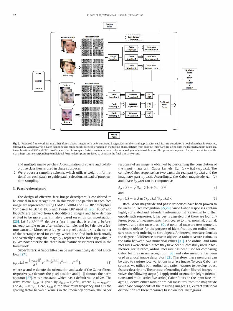
.2. Histogram of Gabor Ordinal Ratio Measures (HGORM)

To code Gabor phase responses, we use the Ordinal Measure (OM)

30,33] . OM compares two different regions to determine which one

as a larger value (e.g., mean). For instance, if region A has a larger

alue than region B, then the resulting code is 1, otherwise it is 0. Such

measure is used to encode the qualitative relationship between dif-

erent regions. The advantages of using ordinal measures for image

epresentation have been established in palmprint recognition [33] ,

ris recognition [30] and face recognition [4] . To perform ordinal fea-

ure extraction, one simple approach is to compute the weighted av-

rage of dissociated image regions. This can be accomplished by the

rocess of ordinal filtering. An ordinal filter consists of multiple posi-

ive and negative lobes, as illustrated in Fig. 3 . Here, we use multi-lobe

ifferential filters (MLDF) [4] to extract ordinal features. The positive

nd negative lobes are represented by Gaussian filters. MLDF can be

athematically expressed as,

LDF = C p

N p ∑

i =1

1 √

2 πδpi

exp

[−(z − μpi )

2

2 δ2 pi

]

−C n

N n ∑

j=1

1 √

2 πδn j

exp

[−(z − μn j )

2

2 δ2 n j

], (7)

here z denotes the pixel position, μ and δ denote the central posi-

ion and the scale of a 2D Gaussian filter, respectively. N p is the num-

er of positive lobes and N n is the number of negative lobes. C p and C n re the constant coefficients, used to ensure that the output of MLDF

s zero, i.e., C p N p = C n N n . MLDF is a type of differential bandpass filter.

t is flexible in terms of types of lobes, spatial configuration of lobes,

nd number of lobes. An example of MLDF filters is shown in Fig. 3 .

Unlike the work of Chai et al. [4] , we also consider the ratio mea-

ure in addition to the ordinal measure. First, we construct a horizon-

al di-lobe ordinal filter and a vertical di-lobe ordinal filter. Then, we

erform the ordinal filtering on the output of Gabor phase responses.

inally, a ratio measure is used to compute the final representation,

hich is denoted as OF:

F = arctan

(β · O v

O + λ

), (8)

h i

here O h is the convolution of horizontal di-lobe ordinal filter with

he Gabor phase response and O v is the convolution of vertical di-

obe ordinal filter with the Gabor phase response. β and λ are con-

tant values used to stabilize the function. The domain of Eq. (8) is

−∞ , + ∞ ]. The proposed feature representation is called Histogram

f Gabor Ordinal Ratio Measures (HGORM). We use the following pa-

ameters in our work: the size of the ordinal filter is 21, the distance

etween positive and negative lobes is 3 pixels, δpi = δn j = π/ 2 , N p = n = 1 , β = 3 and λ = 1 × 10 −7 .

HGORM can be considered as an extension of the LGGP descriptor

hat we previously developed [26] . The ratio measure used in HGORM

s weighted by a Gaussian kernel, thereby making it more robust to

oise. To generate HGORM features, each OM-encoded Gabor image

s divided into non-overlapping patches, where histogram information

s extracted from each patch. The number of patches in each image is

4, where each patch size is 16 × 16. The number of histogram bins is

6. HGORM feature extraction is denoted as f O (I) = { o 1 , o 2 , . . . , o P } ,here P is the number of total patches and o p ∈ R

16 .

.3. Densely Sampled Local Binary Pattern (DS-LBP)

The LBP texture descriptor [27] has been proven to be effective

n capturing micro-patterns or micro-structures in the face image. It

s calculated by binarizing local neighborhoods, based on the differ-

nces in pixel intensity between the center pixel and neighborhood

ixels, and converting the resulting binary string into a decimal value.

n this work, uniform LBP patterns are extracted from the original im-

ge, resulting in a 59-bin histogram feature vector. Uniform LBP pat-

erns refer to those binary patterns that have at most two bitwise

ransitions from 0 to 1 or 1 to 0. Uniformity is an important char-

cteristic, as it reflects micro-features such as lines, edges and cor-

ers, which are enhanced by the application of makeup. To gener-

te DS-LBP features, each LBP coded image is divided into overlapping

atches, and histogram information is extracted from each patch. The

umber of patches in each image is 256, where each patch size is 16

16. The number of histogram bins is 59. DS-LBP feature extraction

s denoted as f (I) = { s , s , . . . , s } , where P is the number of total

S 1 2 P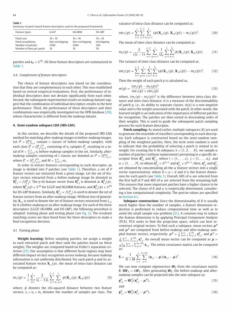

84 C. Chen et al. / Information Fusion 32 (2016) 80–92

Table 1

Summary of patch-based feature descriptors used in the proposed framework.

Feature types LGGP HGORM DS-LBP

Patch size 16 ∗ 16 16 ∗ 16 16 ∗ 16

Patch tessellation Non-overlapping Non-overlapping Overlapping

Number of patches 2560 2560 256

Number of bins per patch 16 16 59

v

v

T

m

T

v

T

w

w

t

o

v

l

f

t

p

t

t

p

t

w

n

s

α

a

v

s

t

T

s

i

i

m

d

a

t

(

c

a

p

a

S

W

S

m

y

a

y

patches and s p ∈ R

59 . All three feature descriptors are summarized in

Table 1 .

3.4. Complement of feature descriptors

The choice of feature descriptors was based on the considera-

tion that they are complementary to each other. This was established

based on several empirical evaluations. First, the performance of in-

dividual descriptors does not deviate significantly from each other.

Second, the subsequent experimental results on makeup dataset sug-

gest that the combination of individual descriptors results in the best

performance. Third, the performance of these descriptors and their

combinations was empirically investigated on the HFB database [26] ,

whose characteristic is different from the makeup dataset.

4. Semi-random subspace LDA (SRS-LDA)

In this section, we describe the details of the proposed SRS-LDA

method for matching after-makeup images to before-makeup images.

Let I B = { I B i } c

i =1 contain c classes of before-makeup samples, with

each class I B i

= { I B i, j

} n i j=1

consisting of n i samples I B i, j

resulting in a to-

tal of N =

∑ c i =1 n i before-makeup samples in the set. Similarly, after-

makeup samples consisting of c classes are denoted as I A = { I A i } c

i =1 ,

where I A i

= { I A i, j

} m i j=1

and M =

∑ c i =1 m i .

In order to extract features corresponding to each descriptor, an

image is divided into P patches (see Table 1 ). Therefore, a set of P

feature vectors are extracted from a given image. Let the set of fea-

ture vectors extracted from a before-makeup image be denoted as

X

B i, j = f (I B

i, j ). The p -th feature vector from X

B i, j is denoted as X

B i, j (p),

where X

B i, j (p) ∈ R

16 for LGGP and HGORM features, and X

B i, j (p) ∈ R

59

for DS-LBP features. Similarly, X

A i, j = f (I A

i, j ) is used to denote the set of

feature vectors from an after-makeup image. Without loss of general-

ity, X i, j is used to denote the set of feature vectors extracted from I i, j ,

be it a before-makeup or an after-makeup image. For each of the three

descriptors (LGGP, HGORM, and DS-LBP), the following procedure is

adopted: training phase and testing phase (see Fig. 2 ). The resultant

matching scores are then fused from the three descriptors to make a

final recognition decision.

4.1. Training phase

Weight learning: Before sampling patches, we assign a weight

to each extracted patch and then rank the patches based on these

weights. The weights are computed based on Fisher’s separation cri-

terion [27] . Our assumption is that different facial regions may have

different im pact on face recognition across makeup, because makeup

information is not uniformly distributed. For each patch p and its as-

sociated feature vector X i, j (p), the mean of intra-class distance can

be computed as:

m 1 (p) =

1

c

c ∑

i =1

2

(l i − 1 )l i

l i −1 ∑

j=1

l i ∑

k = j+1

φ(X i, j (p), X i,k (p)) (9)

where, φ denotes the chi-squared distance between two feature

vectors, l = n + m denotes the number of samples per class. The

i i i

ariance of intra-class distance can be computed as:

ar 1 (p) =

c ∑

i =1

l i −1 ∑

j=1

l i ∑

k = j+1

(φ(X i, j (p), X i,k (p)) − m 1 (p))2 . (10)

he mean of inter-class distance can be computed as:

2 (p) =

2

c(c − 1 )

c−1 ∑

i =1

c ∑

q = i +1

1

l i l q

l i ∑

j=1

l q ∑

k =1

φ(X i, j (p), X i,k (p)). (11)

he variance of inter-class distance can be computed as:

ar 2 (p) =

c−1 ∑

i =1

c ∑

q = i +1

l i ∑

j=1

l q ∑

k =1

(φ(X i, j (p), X i,k (p)) − m 2 (p))2 . (12)

hen the weight of each patch p is calculated as,

(p) =

(m 1 (p) − m 2 (p))2

v ar 1 (p) + v ar 2 (p)(13)

here, (m 1 (p) − m 2 (p))2 is the difference between intra-class dis-

ance and inter-class distance. It is a measure of the discriminability

f patch p , i.e., its ability to separate classes. w ( p ) is a non-negative

alue and is the weight associated with the patch. In other words, the

earned weight is an indication of the importance of different patches

or recognition. The patches are then sorted in descending order of

heir weights. This is used to guide the subsequent patch sampling

rocess for each feature descriptor.

Patch sampling: As stated earlier, multiple subspaces ( K ) are used

o generate the ensemble of classifiers corresponding to each descrip-

or. Each subspace is constructed based on the semi-random sam-

ling of the weighted patches. Here, the term semi-random is used

o indicate that the probability of selecting a patch is related to its

eight. For creating the k -th subspace, k = { 1 , 2 , . . . K} , we sample αumber of patches (without replacement) pertaining to a specific de-

criptor from X

B i, j and X

A i, j , where i = { 1 , . . . , c} , j = { 1 , . . . , n i } , and

∈ { 1 , . . . , P } , to obtain x B i, j

∈ R

D ×1 and x A i, j

∈ R

D ×1 . Here, x B i, j

and x A i, j

re obtained by concatenating all the α feature vectors into a single

ector representation, where D = α × d and d is the feature dimen-

ion for each patch (see Table 1 ). Overall, 60% of α are selected from

he first half of P and 40% of α are selected from the remaining half.

his ensures that more important patches have a higher chance to be

elected. The choice of K and α is empirically determined, consider-

ng a low computational complexity. The precise values are specified

n Section 6.1 .

Subspace construction: Since the dimensionality of D is usually

uch higher than the number of samples, a feature dimension re-

uction is performed to reduce computational time as well as to

void the small sample size problem [21] . A common way to reduce

he feature dimension is by applying Principal Component Analysis

PCA). PCA seeks to find the projection space, which can best re-

onstruct original vectors. To find such a subspace, mean vectors μB

nd μA are computed from before-makeup and after-makeup sam-

led feature vectors, respectively: μB =

1 N

∑ c i =1

∑ n i j=1

x B i, j

, and μA =1 M

∑ c i =1

∑ m i j=1

x A i, j

. An overall mean vector can be computed as μ =1

N+ M

∑ c i =1

∑ n i + m i j=1

x i, j . The entire covariance matrix can be computed

s:

=

1

N + M

c ∑

i =1

n i + m i ∑

j=1

(x i, j − μ)(x i, j − μ)T . (14)

e can now compute eigenvectors W E from the covariance matrix

: S W E = λW E . After generating W E , the before-makeup and after-

akeup samples can be projected into the new subspace as:

B i, j = W

T E (x

B i, j − μB ), (15)

nd

A i, j = W

T E (x

A i, j − μA ). (16)

C. Chen et al. / Information Fusion 32 (2016) 80–92 85

y

m

e

c

T

t

s

b

μ

T

S

w

p

S

T

m

t

o

W

T

S

t

T

b

i

b

t

s

p

4

s

m

d

a

p

X

o

t

t

m

y

a

y

w

m

m

c

c

i

b

a

{

g

n

t

t

a

m

t

e

b

m

Z

s

l

f

b

c

d

t

t

t

ρ

a

ρ

T

r

m

T

c

(

ρ

ρ

a

(

e

t

s

u

s

s

s

v

t

t

w

r

E

c

e

B i, j

and y A i, j

are the projected feature vectors after PCA for before-

akeup and after-makeup samples, respectively. The number of

igenvectors used is min (N − c, M − c).

We use both before-makeup and after-makeup feature vectors to

ompute the between-class scatter and within-class scatter matrices.

his ensures that the learned feature representation is less sensitive

o makeup changes. The mean class vector for i -th subject when con-

tructing the k -th subspace for a feature descriptor is calculated using

oth before-makeup ( y B i, j

) and after-makeup ( y A i, j

) projected vectors:

(k)i

=

1

n i + m i

(

n i ∑

j=1

y B i, j +

m i ∑

j=1

y A i, j

)

. (17)

hen the between-class scatter matrix can be computed as,

(k)B

=

c ∑

i =1

(μ(k)i

− μ(k))(μ(k)i

− μ(k))T . (18)

here μ(k) =

1 c

c ∑

i =1

μ(k)i

. The within-class scatter matrix can be com-

uted as,

(k)W

=

c ∑

i =1

n i ∑

j=1

(y B i, j − μ(k)

i

)(y B i, j − μ(k)

i

)T

+

c ∑

i =1

m i ∑

j=1

(y A i, j − μ(k)

i )(y A i, j − μ(k)

i

)T . (19)

he objective of LDA is to seek the optimal projection W F , which can

aximize the ratio between determinant of the between-class scat-

er matrix and determinant of the within-class scatter matrix. The

ptimization problem is defined as,

(k)F

= arg max W F

W

T F S

(k)B

W F

W

T F S

(k)W

W F

. (20)

his is equivalent to solving the generalized eigenvalue problem of

(k)B

ψ

(k) = λ(k)S (k)W

ψ

(k), where k = { 1 , 2 , . . . , K} . The output of the

raining phase is μB , μA , W

(k)F

and W E for each k (i.e., subspace).

he potential importance of this proposed method lies in (a) using

oth before- and after-makeup patches together in the weight learn-

ng process and (b) generating the corresponding subspaces, where

oth before- and after-makeup feature vectors are used for learning

he within- and between-class scatter matrices of LDA. These con-

tructed subspaces, also referred to as common subspaces, are re-

eated for each descriptor.

.2. Testing phase

In the testing phase, the after-makeup images of a subject in a

equestered test set are treated as probes and compared with before-

akeup images that are treated as gallery images. Let X i, j = f (I i, j )enote the set of feature vectors extracted from I i, j , where I i, j is either

before-makeup image or an after-makeup image from test sam-

les. The same set of α patches are selected from { X i, j (p) : X i, j (p) ∈ i, j , 1 < p < P } , and concatenated to form a single feature vector x B

i, j

r x A i, j

. The location and order of patches in the training set and the

est set are the same.

Subspace projection: For each derived subspace k = { 1 , 2 , . . . , K} ,he representation for test samples of before-makeup and after-

akeup are obtained as follows:

B i, j = W

T F W

T E

(x

B i, j − μB

), (21)

nd

A i, j = W

T F W

T E

(x

A i, j − μA

), (22)

here y B i, j

and y A i, j

are the final projected feature vectors for before-

akeup and after-makeup test samples, respectively. In case the

akeup information is unknown, a makeup detection scheme [15]

an be employed to make the distinction. An overall mean vector μan also be used for projection, resulting in a slight decrease in match-

ng accuracy ( < 1% verfication rate).

SRC and CRC classification: As stated earlier, the

efore-makeup samples are used as gallery, and the

fter-makeup samples are used as probe. Let Y

B = y B 1 , 1 , . . . , y

B 1 ,n ′

1

, . . . , y B i, 1

, . . . , y B i,n ′

i

, . . . , y B c ′ , 1 , . . . , y

B c ′ ,n ′ c

} denote the

allery feature vectors of before-makeup samples, where c ′ is the

umber of subjects in the gallery and n ′ i

is the number of samples for

he i -th subject. Let y A i, j

denote an after-makeup probe sample. Dis-

ance scores can be computed by matching a probe sample against

gallery, thereby obtaining a similarity score between before-

akeup and after-makeup samples. This is accomplished by using

he principles of sparse and collaborative representation. Wright

t al. [42] demonstrated the robustness of sparse representation

ased classification (SRC) to occlusions and noise. The application of

akeup can be viewed as the addition of noise, i.e., pixel corruption.

hang et al. [34] demonstrated that it is the collaborative repre-

entation based classification (CRC), rather than just sparsity, that

ends robustness to face recognition. Thus, the collaborative role of

ace images from other subjects in the classification process cannot

e undermined. SRC and CRC have their own merits and can provide

omplementary information in classification [34] . Therefore, we

evelop two classifiers for each subspace – one based on SRC and

he other on CRC – and combine their outputs. In this way, we exploit

he complementary information provided by both of them.

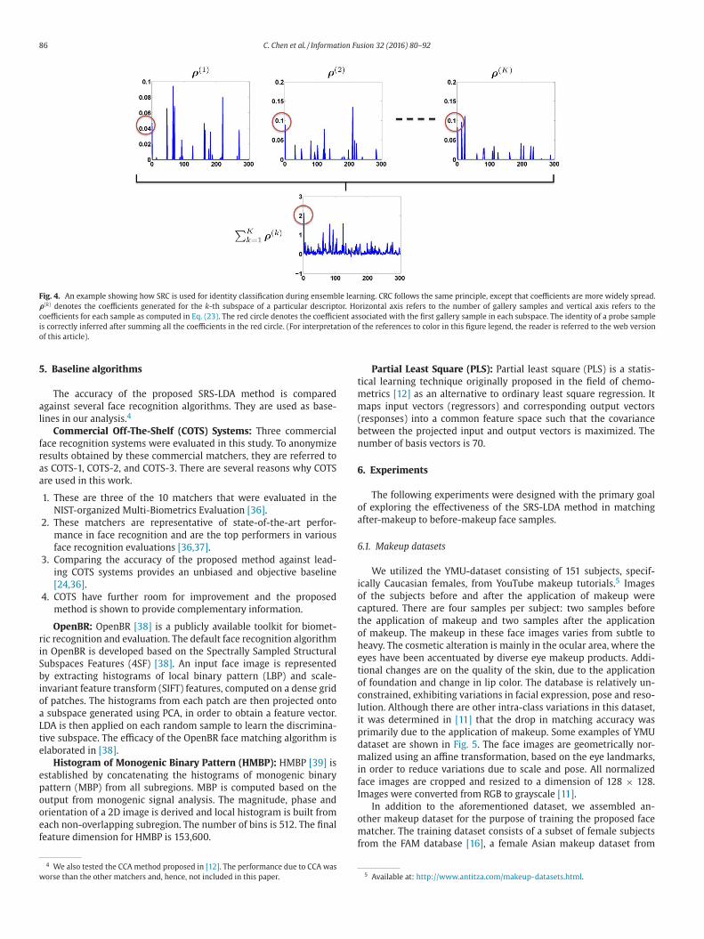
The coefficient of projection of an after-makeup sample can be ob-

ained using both � 1 (SRC) and � 2 (CRC) solutions:

(k)1

= arg min

ρ|| Y

B ρ − y A i, j || 2 2 + λ1 || ρ|| 1 , (23)

nd

(k)2

= ((Y

B )T Y

B + λ2 I )−1 (Y

B )T (y A i, j

). (24)

he � 1 solution is obtained using Least Angle Regression (LARS) algo-

ithm [35] . LARS algorithm is a variant for solving the Lasso based on

odel selection. The dimension of both ρ(k)1

and ρ(k)2

is N

′ =

∑ c ′ i =1 n

′ i .

he coefficient vector for the k -th subspace is ρ(k) = ρ(k)1

+ ρ(k)2

. The

oefficient vectors pertaining to all subspaces are summed together

see Fig. 4 ):

=

K ∑

k =1

ρ(k). (25)

is the final coefficient (score) vector generated when matching an

fter-makeup feature vector y A i, j

(probe) to a set of feature vectors Y

B

gallery). The proposed framework fuses the output of three differ-

nt feature descriptors, i.e., LGGP, HGORM, and DS-LBP. So there are

hree coefficient vectors: ρG , ρO and ρS . These are combined to get a

ingle coefficient vector ρF = (ρG + ρO + ρS )/ 3 . Here, same weight is

sed for different modalities during the sum-rule fusion. The match

core between the r -th entry in the gallery and the probe image corre-

ponds to the r -th element in ρF . Fig. 4 illustrates this. Given a probe

ample, the red circle denotes the computed coefficient (similarity

alue) associated with the first gallery sample in each subspace. In

his example, the first gallery sample corresponds to the same iden-

ity as the probe sample. The rest of the coefficients are associated

ith other gallery samples. The identity of the probe sample is cor-

ectly inferred after summing all the coefficients in the red circle.

ven though the first gallery sample is not associated with the largest

oefficient value in individual subspaces, the sum of each of these co-

fficients results in the maximum value among all samples.

86 C. Chen et al. / Information Fusion 32 (2016) 80–92

Fig. 4. An example showing how SRC is used for identity classification during ensemble learning. CRC follows the same principle, except that coefficients are more widely spread.

ρ( k ) denotes the coefficients generated for the k -th subspace of a particular descriptor. Horizontal axis refers to the number of gallery samples and vertical axis refers to the

coefficients for each sample as computed in Eq. (23) . The red circle denotes the coefficient associated with the first gallery sample in each subspace. The identity of a probe sample

is correctly inferred after summing all the coefficients in the red circle. (For interpretation of the references to color in this figure legend, the reader is referred to the web version

of this article).

t

m

m

(

b

n

6

o

a

6

i

o

c

t

o

h

e

t

o

c

l

i

p

d

m

i

f

I

o

m

5. Baseline algorithms

The accuracy of the proposed SRS-LDA method is compared

against several face recognition algorithms. They are used as base-

lines in our analysis. 4

Commercial Off-The-Shelf (COTS) Systems: Three commercial

face recognition systems were evaluated in this study. To anonymize

results obtained by these commercial matchers, they are referred to

as COTS-1, COTS-2, and COTS-3. There are several reasons why COTS

are used in this work.

1. These are three of the 10 matchers that were evaluated in the

NIST-organized Multi-Biometrics Evaluation [36] .

2. These matchers are representative of state-of-the-art perfor-

mance in face recognition and are the top performers in various

face recognition evaluations [36,37] .

3. Comparing the accuracy of the proposed method against lead-

ing COTS systems provides an unbiased and objective baseline

[24,36] .

4. COTS have further room for improvement and the proposed

method is shown to provide complementary information.

OpenBR: OpenBR [38] is a publicly available toolkit for biomet-

ric recognition and evaluation. The default face recognition algorithm

in OpenBR is developed based on the Spectrally Sampled Structural

Subspaces Features (4SF) [38] . An input face image is represented

by extracting histograms of local binary pattern (LBP) and scale-

invariant feature transform (SIFT) features, computed on a dense grid

of patches. The histograms from each patch are then projected onto

a subspace generated using PCA, in order to obtain a feature vector.

LDA is then applied on each random sample to learn the discrimina-

tive subspace. The efficacy of the OpenBR face matching algorithm is

elaborated in [38] .

Histogram of Monogenic Binary Pattern (HMBP): HMBP [39] is

established by concatenating the histograms of monogenic binary

pattern (MBP) from all subregions. MBP is computed based on the

output from monogenic signal analysis. The magnitude, phase and

orientation of a 2D image is derived and local histogram is built from

each non-overlapping subregion. The number of bins is 512. The final

feature dimension for HMBP is 153,600.

4 We also tested the CCA method proposed in [12] . The performance due to CCA was

worse than the other matchers and, hence, not included in this paper.

f

Partial Least Square (PLS): Partial least square (PLS) is a statis-

ical learning technique originally proposed in the field of chemo-

etrics [12] as an alternative to ordinary least square regression. It

aps input vectors (regressors) and corresponding output vectors

responses) into a common feature space such that the covariance

etween the projected input and output vectors is maximized. The

umber of basis vectors is 70.

. Experiments

The following experiments were designed with the primary goal

f exploring the effectiveness of the SRS-LDA method in matching

fter-makeup to before-makeup face samples.

.1. Makeup datasets

We utilized the YMU-dataset consisting of 151 subjects, specif-

cally Caucasian females, from YouTube makeup tutorials. 5 Images

f the subjects before and after the application of makeup were

aptured. There are four samples per subject: two samples before

he application of makeup and two samples after the application

f makeup. The makeup in these face images varies from subtle to

eavy. The cosmetic alteration is mainly in the ocular area, where the

yes have been accentuated by diverse eye makeup products. Addi-

ional changes are on the quality of the skin, due to the application

f foundation and change in lip color. The database is relatively un-

onstrained, exhibiting variations in facial expression, pose and reso-

ution. Although there are other intra-class variations in this dataset,

t was determined in [11] that the drop in matching accuracy was

rimarily due to the application of makeup. Some examples of YMU

ataset are shown in Fig. 5 . The face images are geometrically nor-

alized using an affine transformation, based on the eye landmarks,

n order to reduce variations due to scale and pose. All normalized

ace images are cropped and resized to a dimension of 128 × 128.

mages were converted from RGB to grayscale [11] .

In addition to the aforementioned dataset, we assembled an-

ther makeup dataset for the purpose of training the proposed face

atcher. The training dataset consists of a subset of female subjects

rom the FAM database [16] , a female Asian makeup dataset from

5 Available at: http://www.antitza.com/makeup-datasets.html .

C. Chen et al. / Information Fusion 32 (2016) 80–92 87

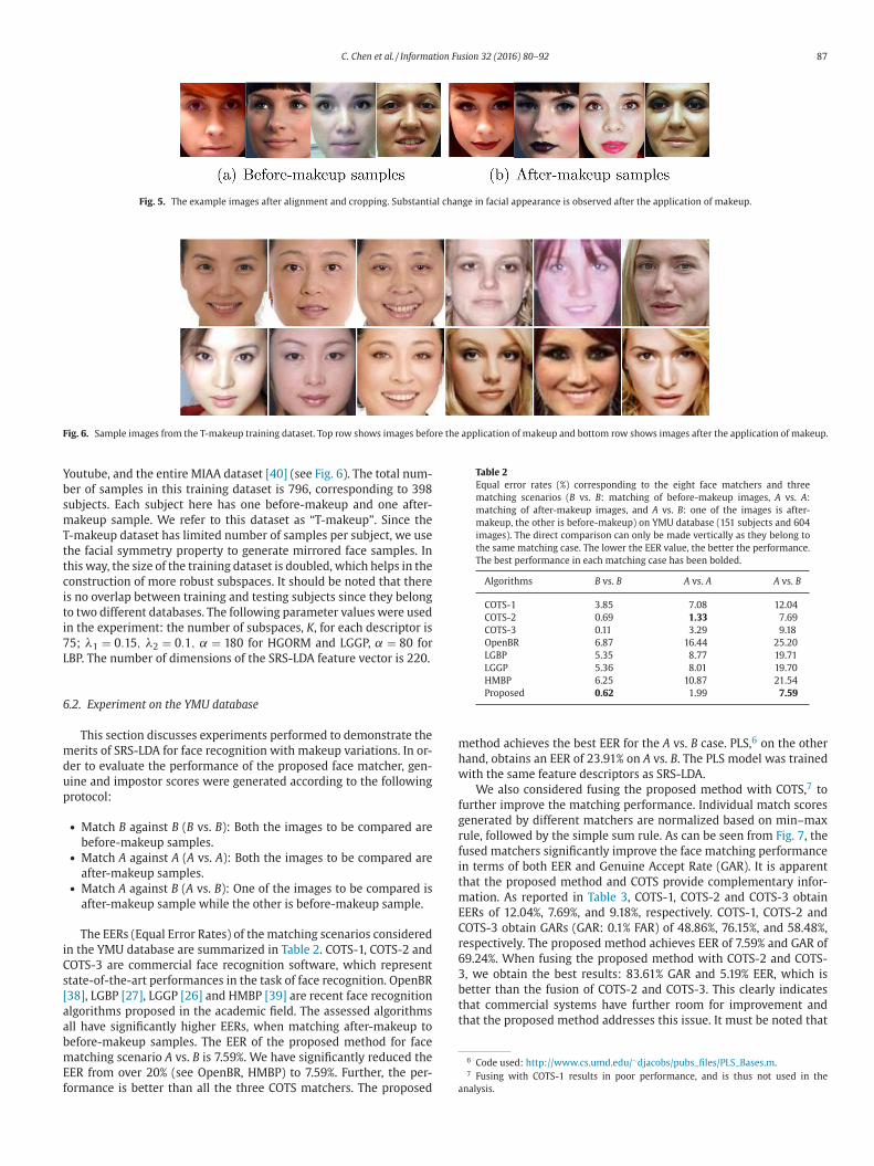
Fig. 5. The example images after alignment and cropping. Substantial change in facial appearance is observed after the application of makeup.

Fig. 6. Sample images from the T-makeup training dataset. Top row shows images before the application of makeup and bottom row shows images after the application of makeup.

Y

b

s

m

T

t

t

c

i

t

i

7

L

6

m

d

u

p

i

C

s

[

a

a

b

m

E

f

Table 2

Equal error rates (%) corresponding to the eight face matchers and three

matching scenarios ( B vs. B : matching of before-makeup images, A vs. A :

matching of after-makeup images, and A vs. B : one of the images is after-

makeup, the other is before-makeup) on YMU database (151 subjects and 604

images). The direct comparison can only be made vertically as they belong to

the same matching case. The lower the EER value, the better the performance.

The best performance in each matching case has been bolded.

Algorithms B vs. B A vs. A A vs. B

COTS-1 3.85 7 .08 12 .04

COTS-2 0.69 1 .33 7 .69

COTS-3 0.11 3 .29 9 .18

OpenBR 6.87 16 .44 25 .20

LGBP 5.35 8 .77 19 .71

LGGP 5.36 8 .01 19 .70

HMBP 6.25 10 .87 21 .54

Proposed 0.62 1 .99 7 .59

m

h

w

f

g

r

f

i

t

m

E

C

r

6

3

b

t

t

6 Code used: http://www.cs.umd.edu/ ∼djacobs/pubs _ files/PLS _ Bases.m . 7 Fusing with COTS-1 results in poor performance, and is thus not used in the

analysis.

outube, and the entire MIAA dataset [40] (see Fig. 6 ). The total num-

er of samples in this training dataset is 796, corresponding to 398

ubjects. Each subject here has one before-makeup and one after-

akeup sample. We refer to this dataset as “T-makeup”. Since the

-makeup dataset has limited number of samples per subject, we use

he facial symmetry property to generate mirrored face samples. In

his way, the size of the training dataset is doubled, which helps in the

onstruction of more robust subspaces. It should be noted that there

s no overlap between training and testing subjects since they belong

o two different databases. The following parameter values were used

n the experiment: the number of subspaces, K , for each descriptor is

5; λ1 = 0 . 15 , λ2 = 0 . 1 , α = 180 for HGORM and LGGP, α = 80 for

BP. The number of dimensions of the SRS-LDA feature vector is 220.

.2. Experiment on the YMU database

This section discusses experiments performed to demonstrate the

erits of SRS-LDA for face recognition with makeup variations. In or-

er to evaluate the performance of the proposed face matcher, gen-

ine and impostor scores were generated according to the following

rotocol:

• Match B against B ( B vs. B ): Both the images to be compared are

before-makeup samples. • Match A against A ( A vs. A ): Both the images to be compared are

after-makeup samples. • Match A against B ( A vs. B ): One of the images to be compared is

after-makeup sample while the other is before-makeup sample.

The EERs (Equal Error Rates) of the matching scenarios considered

n the YMU database are summarized in Table 2 . COTS-1, COTS-2 and

OTS-3 are commercial face recognition software, which represent

tate-of-the-art performances in the task of face recognition. OpenBR

38] , LGBP [27] , LGGP [26] and HMBP [39] are recent face recognition

lgorithms proposed in the academic field. The assessed algorithms

ll have significantly higher EERs, when matching after-makeup to

efore-makeup samples. The EER of the proposed method for face

atching scenario A vs. B is 7.59%. We have significantly reduced the

ER from over 20% (see OpenBR, HMBP) to 7.59%. Further, the per-

ormance is better than all the three COTS matchers. The proposed

ethod achieves the best EER for the A vs. B case. PLS, 6 on the other

and, obtains an EER of 23.91% on A vs. B . The PLS model was trained

ith the same feature descriptors as SRS-LDA.

We also considered fusing the proposed method with COTS, 7 to

urther improve the matching performance. Individual match scores

enerated by different matchers are normalized based on min–max

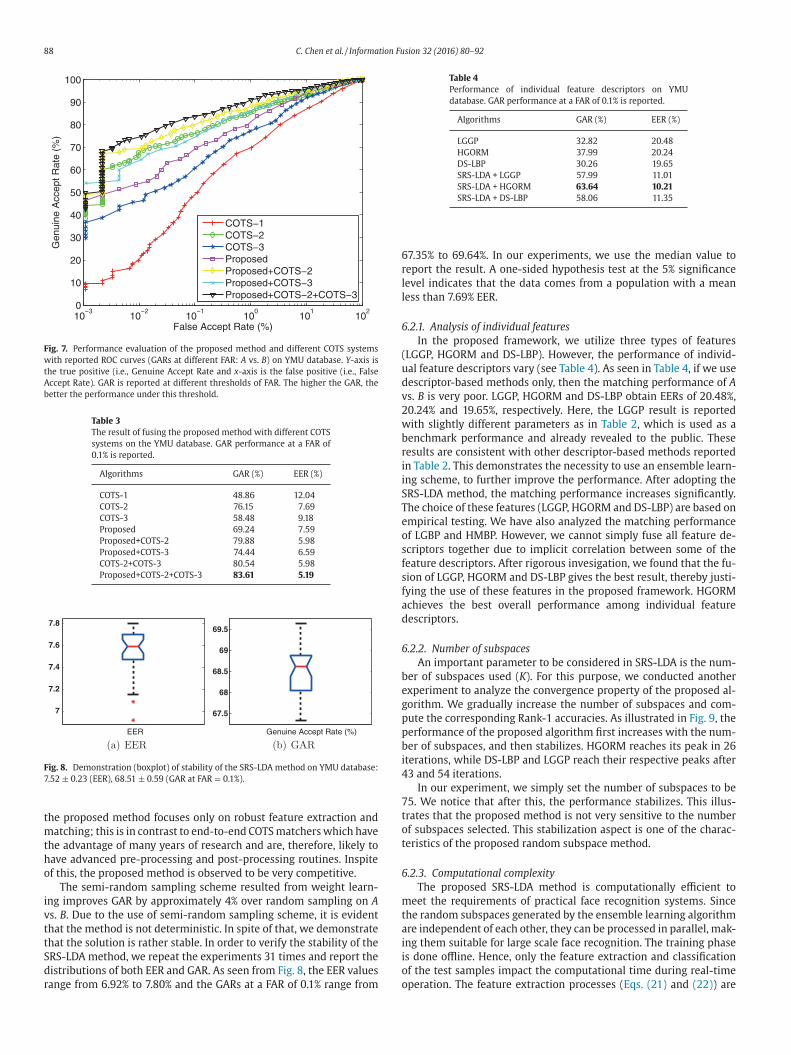
ule, followed by the simple sum rule. As can be seen from Fig. 7 , the

used matchers significantly improve the face matching performance

n terms of both EER and Genuine Accept Rate (GAR). It is apparent

hat the proposed method and COTS provide complementary infor-

ation. As reported in Table 3 , COTS-1, COTS-2 and COTS-3 obtain

ERs of 12.04%, 7.69%, and 9.18%, respectively. COTS-1, COTS-2 and

OTS-3 obtain GARs (GAR: 0.1% FAR) of 48.86%, 76.15%, and 58.48%,

espectively. The proposed method achieves EER of 7.59% and GAR of

9.24%. When fusing the proposed method with COTS-2 and COTS-

, we obtain the best results: 83.61% GAR and 5.19% EER, which is

etter than the fusion of COTS-2 and COTS-3. This clearly indicates

hat commercial systems have further room for improvement and

hat the proposed method addresses this issue. It must be noted that

88 C. Chen et al. / Information Fusion 32 (2016) 80–92

10−3

10−2

10−1

100

101

102

0

10

20

30

40

50

60

70

80

90

100

False Accept Rate (%)

Gen

uine

Acc

ept R

ate

(%)

COTS−1COTS−2COTS−3ProposedProposed+COTS−2Proposed+COTS−3Proposed+COTS−2+COTS−3

Fig. 7. Performance evaluation of the proposed method and different COTS systems

with reported ROC curves (GARs at different FAR: A vs. B ) on YMU database. Y -axis is

the true positive (i.e., Genuine Accept Rate and x -axis is the false positive (i.e., False

Accept Rate). GAR is reported at different thresholds of FAR. The higher the GAR, the

better the performance under this threshold.

Table 3

The result of fusing the proposed method with different COTS

systems on the YMU database. GAR performance at a FAR of

0.1% is reported.

Algorithms GAR (%) EER (%)

COTS-1 48 .86 12 .04

COTS-2 76 .15 7 .69

COTS-3 58 .48 9 .18

Proposed 69 .24 7 .59

Proposed+COTS-2 79 .88 5 .98

Proposed+COTS-3 74 .44 6 .59

COTS-2+COTS-3 80 .54 5 .98

Proposed+COTS-2+COTS-3 83 .61 5 .19

7

7.2

7.4

7.6

7.8

EER

(a) EER

67.5

68

68.5

69

69.5

Genuine Accept Rate (%)

(b) GAR

Fig. 8. Demonstration (boxplot) of stability of the SRS-LDA method on YMU database:

7.52 ± 0.23 (EER), 68.51 ± 0.59 (GAR at FAR = 0.1%).

Table 4

Performance of individual feature descriptors on YMU

database. GAR performance at a FAR of 0.1% is reported.

Algorithms GAR (%) EER (%)

LGGP 32 .82 20 .48

HGORM 37 .99 20 .24

DS-LBP 30 .26 19 .65

SRS-LDA + LGGP 57 .99 11 .01

SRS-LDA + HGORM 63 .64 10 .21

SRS-LDA + DS-LBP 58 .06 11 .35

6

r

l

l

6

(

u

d

v

2

w

b

r

i

i

S

T

e

o

s

f

s

f

a

d

6

b

e

g

p

p

b

i

4

7

t

o

t

6

m

t

a

i

i

o

o

the proposed method focuses only on robust feature extraction and

matching; this is in contrast to end-to-end COTS matchers which have

the advantage of many years of research and are, therefore, likely to

have advanced pre-processing and post-processing routines. Inspite

of this, the proposed method is observed to be very competitive.

The semi-random sampling scheme resulted from weight learn-

ing improves GAR by approximately 4% over random sampling on A

vs. B . Due to the use of semi-random sampling scheme, it is evident

that the method is not deterministic. In spite of that, we demonstrate

that the solution is rather stable. In order to verify the stability of the

SRS-LDA method, we repeat the experiments 31 times and report the

distributions of both EER and GAR. As seen from Fig. 8 , the EER values

range from 6.92% to 7.80% and the GARs at a FAR of 0.1% range from

7.35% to 69.64%. In our experiments, we use the median value to

eport the result. A one-sided hypothesis test at the 5% significance

evel indicates that the data comes from a population with a mean

ess than 7.69% EER.

.2.1. Analysis of individual features

In the proposed framework, we utilize three types of features

LGGP, HGORM and DS-LBP). However, the performance of individ-

al feature descriptors vary (see Table 4 ). As seen in Table 4 , if we use

escriptor-based methods only, then the matching performance of A

s. B is very poor. LGGP, HGORM and DS-LBP obtain EERs of 20.48%,

0.24% and 19.65%, respectively. Here, the LGGP result is reported

ith slightly different parameters as in Table 2 , which is used as a

enchmark performance and already revealed to the public. These

esults are consistent with other descriptor-based methods reported

n Table 2 . This demonstrates the necessity to use an ensemble learn-

ng scheme, to further improve the performance. After adopting the

RS-LDA method, the matching performance increases significantly.

he choice of these features (LGGP, HGORM and DS-LBP) are based on

mpirical testing. We have also analyzed the matching performance

f LGBP and HMBP. However, we cannot simply fuse all feature de-

criptors together due to implicit correlation between some of the

eature descriptors. After rigorous invesigation, we found that the fu-

ion of LGGP, HGORM and DS-LBP gives the best result, thereby justi-

ying the use of these features in the proposed framework. HGORM

chieves the best overall performance among individual feature

escriptors.

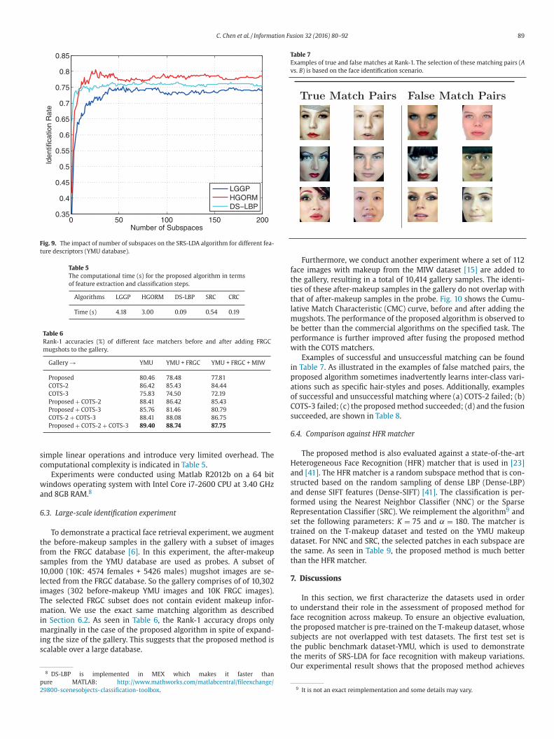
.2.2. Number of subspaces

An important parameter to be considered in SRS-LDA is the num-

er of subspaces used ( K ). For this purpose, we conducted another

xperiment to analyze the convergence property of the proposed al-

orithm. We gradually increase the number of subspaces and com-

ute the corresponding Rank-1 accuracies. As illustrated in Fig. 9 , the

erformance of the proposed algorithm first increases with the num-

er of subspaces, and then stabilizes. HGORM reaches its peak in 26

terations, while DS-LBP and LGGP reach their respective peaks after

3 and 54 iterations.

In our experiment, we simply set the number of subspaces to be

5. We notice that after this, the performance stabilizes. This illus-

rates that the proposed method is not very sensitive to the number

f subspaces selected. This stabilization aspect is one of the charac-

eristics of the proposed random subspace method.

.2.3. Computational complexity

The proposed SRS-LDA method is computationally efficient to

eet the requirements of practical face recognition systems. Since

he random subspaces generated by the ensemble learning algorithm

re independent of each other, they can be processed in parallel, mak-

ng them suitable for large scale face recognition. The training phase

s done offline. Hence, only the feature extraction and classification

f the test samples impact the computational time during real-time

peration. The feature extraction processes ( Eqs. (21) and (22) ) are

C. Chen et al. / Information Fusion 32 (2016) 80–92 89

0 50 100 150 2000.35

0.4

0.45

0.5

0.55

0.6

0.65

0.7

0.75

0.8

0.85

Number of Subspaces

Iden

tific

atio

n R

ate

LGGPHGORMDS−LBP

Fig. 9. The impact of number of subspaces on the SRS-LDA algorithm for different fea-

ture descriptors (YMU database).

Table 5

The computational time (s) for the proposed algorithm in terms

of feature extraction and classification steps.

Algorithms LGGP HGORM DS-LBP SRC CRC

Time (s) 4.18 3.00 0.09 0.54 0.19

Table 6

Rank-1 accuracies (%) of different face matchers before and after adding FRGC

mugshots to the gallery.

Gallery → YMU YMU + FRGC YMU + FRGC + MIW

Proposed 80.46 78.48 77.81

COTS-2 86.42 85.43 84.44

COTS-3 75.83 74.50 72.19

Proposed + COTS- 2 88.41 86.42 85.43

Propose d + COTS- 3 85.76 81.46 80.79

COTS-2 + COTS-3 88.41 88.08 86.75

Proposed + COTS-2 + COTS-3 89.40 88.74 87.75

s

c

w

a

6

t

f

s

1

l

i

T

m

i

m

i

s

p

2

Table 7

Examples of true and false matches at Rank-1. The selection of these matching pairs ( A

vs. B ) is based on the face identification scenario.

True Match Pairs False Match Pairs

f

t

t

t

l

m

b

p

w

i

p

a

o

C

s

6

H

a

s

a

f

R

s

t

d

t

t

7

t

f

t

s

t

imple linear operations and introduce very limited overhead. The

omputational complexity is indicated in Table 5 .

Experiments were conducted using Matlab R2012b on a 64 bit

indows operating system with Intel Core i7-2600 CPU at 3.40 GHz

nd 8GB RAM. 8

.3. Large-scale identification experiment

To demonstrate a practical face retrieval experiment, we augment

he before-makeup samples in the gallery with a subset of images

rom the FRGC database [6] . In this experiment, the after-makeup

amples from the YMU database are used as probes. A subset of

0,0 0 0 (10K: 4574 females + 5426 males) mugshot images are se-

ected from the FRGC database. So the gallery comprises of of 10,302

mages (302 before-makeup YMU images and 10K FRGC images).

he selected FRGC subset does not contain evident makeup infor-

ation. We use the exact same matching algorithm as described

n Section 6.2 . As seen in Table 6 , the Rank-1 accuracy drops only

arginally in the case of the proposed algorithm in spite of expand-

ng the size of the gallery. This suggests that the proposed method is

calable over a large database.

8 DS-LBP is implemented in MEX which makes it faster than

ure MATLAB: http://www.mathworks.com/matlabcentral/fileexchange/

9800- scenesobjects- classification- toolbox .

t

O

Furthermore, we conduct another experiment where a set of 112

ace images with makeup from the MIW dataset [15] are added to

he gallery, resulting in a total of 10,414 gallery samples. The identi-

ies of these after-makeup samples in the gallery do not overlap with

hat of after-makeup samples in the probe. Fig. 10 shows the Cumu-

ative Match Characteristic (CMC) curve, before and after adding the

ugshots. The performance of the proposed algorithm is observed to

e better than the commercial algorithms on the specified task. The

erformance is further improved after fusing the proposed method

ith the COTS matchers.

Examples of successful and unsuccessful matching can be found

n Table 7 . As illustrated in the examples of false matched pairs, the

roposed algorithm sometimes inadvertently learns inter-class vari-

tions such as specific hair-styles and poses. Additionally, examples

f successful and unsuccessful matching where (a) COTS-2 failed; (b)

OTS-3 failed; (c) the proposed method succeeded; (d) and the fusion

ucceeded, are shown in Table 8 .

.4. Comparison against HFR matcher

The proposed method is also evaluated against a state-of-the-art

eterogeneous Face Recognition (HFR) matcher that is used in [23]

nd [41] . The HFR matcher is a random subspace method that is con-

tructed based on the random sampling of dense LBP (Dense-LBP)

nd dense SIFT features (Dense-SIFT) [41] . The classification is per-

ormed using the Nearest Neighbor Classifier (NNC) or the Sparse

epresentation Classifier (SRC). We reimplement the algorithm

9 and

et the following parameters: K = 75 and α = 180 . The matcher is

rained on the T-makeup dataset and tested on the YMU makeup

ataset. For NNC and SRC, the selected patches in each subspace are

he same. As seen in Table 9 , the proposed method is much better

han the HFR matcher.

. Discussions

In this section, we first characterize the datasets used in order

o understand their role in the assessment of proposed method for

ace recognition across makeup. To ensure an objective evaluation,

he proposed matcher is pre-trained on the T-makeup dataset, whose

ubjects are not overlapped with test datasets. The first test set is

he public benchmark dataset-YMU, which is used to demonstrate

he merits of SRS-LDA for face recognition with makeup variations.

ur experimental result shows that the proposed method achieves

9 It is not an exact reimplementation and some details may vary.

90 C. Chen et al. / Information Fusion 32 (2016) 80–92

0 20 40 60 80 1000.7

0.75

0.8

0.85

0.9

0.95

1

Rank

Ide

ntifica

tio

n R

ate

Gallery: YMU only

Gallery: YMU+FRGC Mugshots

Gallery: YMU+FRGC Mugshots+MIW

(a) Proposed (SRS-LDA)

0 20 40 60 80 1000.7

0.75

0.8

0.85

0.9

0.95

1

Rank

Ide

ntifica

tio

n R

ate

Gallery: YMU only

Gallery: YMU+FRGC Mugshots

Gallery: YMU+FRGC Mugshots+MIW

(b) COTS-2

0 20 40 60 80 1000.7

0.75

0.8

0.85

0.9

0.95

1

Rank

Ide

ntifica

tio

n R

ate

Gallery: YMU only

Gallery: YMU+FRGC Mugshots

Gallery: YMU+FRGC Mugshots+MIW

(c) COTS-3

0 20 40 60 80 1000.7

0.75

0.8

0.85

0.9

0.95

1

Rank

Ide

ntifica

tio

n R

ate

Gallery: YMU only

Gallery: YMU+FRGC Mugshots

Gallery: YMU+FRGC Mugshots+MIW

(d) Proposed+COTS-2

0 20 40 60 80 1000.7

0.75

0.8

0.85

0.9

0.95

1

Rank

Ide

ntifica

tio

n R

ate

Gallery: YMU only

Gallery: YMU+FRGC Mugshots

Gallery: YMU+FRGC Mugshots+MIW

(e) Proposed+COTS-3

0 20 40 60 80 1000.7

0.75

0.8

0.85

0.9

0.95

1

Rank

Ide

ntifica

tio

n R

ate

Gallery: YMU only

Gallery: YMU+FRGC Mugshots

Gallery: YMU+FRGC Mugshots+MIW

(f) Proposed+COTS-2+COTS-3

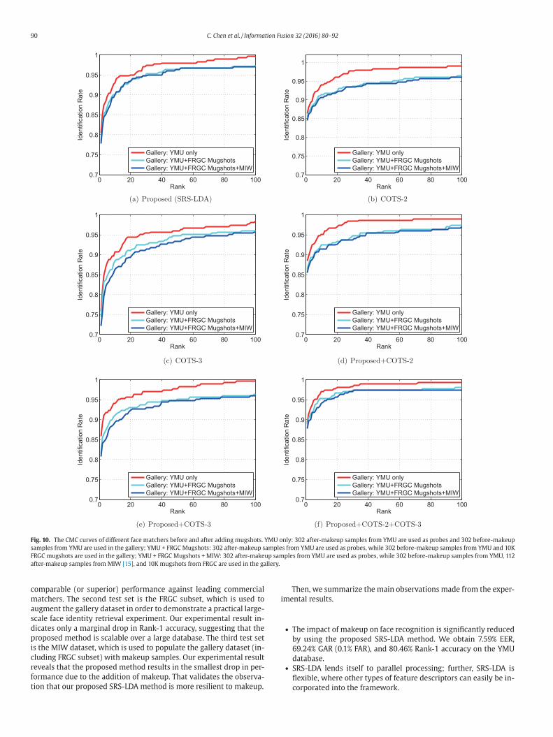
Fig. 10. The CMC curves of different face matchers before and after adding mugshots. YMU only: 302 after-makeup samples from YMU are used as probes and 302 before-makeup

samples from YMU are used in the gallery; YMU + FRGC Mugshots: 302 after-makeup samples from YMU are used as probes, while 302 before-makeup samples from YMU and 10K

FRGC mugshots are used in the gallery; YMU + FRGC Mugshots + MIW: 302 after-makeup samples from YMU are used as probes, while 302 before-makeup samples from YMU, 112

after-makeup samples from MIW [15] , and 10K mugshots from FRGC are used in the gallery.

i

comparable (or superior) performance against leading commercial

matchers. The second test set is the FRGC subset, which is used to

augment the gallery dataset in order to demonstrate a practical large-

scale face identity retrieval experiment. Our experimental result in-

dicates only a marginal drop in Rank-1 accuracy, suggesting that the

proposed method is scalable over a large database. The third test set

is the MIW dataset, which is used to populate the gallery dataset (in-

cluding FRGC subset) with makeup samples. Our experimental result

reveals that the proposed method results in the smallest drop in per-

formance due to the addition of makeup. That validates the observa-

tion that our proposed SRS-LDA method is more resilient to makeup.

Then, we summarize the main observations made from the exper-

mental results.

• The impact of makeup on face recognition is significantly reduced

by using the proposed SRS-LDA method. We obtain 7.59% EER,

69.24% GAR (0.1% FAR), and 80.46% Rank-1 accuracy on the YMU

database. • SRS-LDA lends itself to parallel processing; further, SRS-LDA is

flexible, where other types of feature descriptors can easily be in-

corporated into the framework.

C. Chen et al. / Information Fusion 32 (2016) 80–92 91

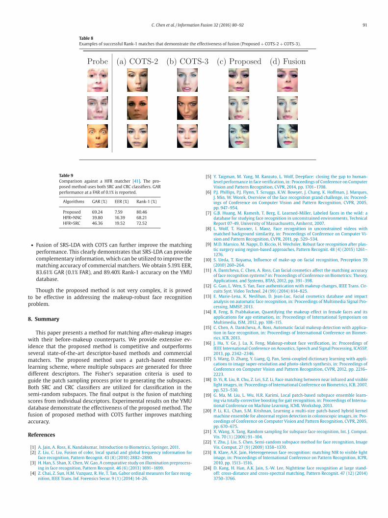
Table 8

Examples of successful Rank-1 matches that demonstrate the effectiveness of fusion ( Proposed + COTS-2 + COTS-3 ).

Probe (a) COTS-2 (b) COTS-3 (c) Proposed (d) Fusion

Table 9

Comparison against a HFR matcher [41] . The pro-

posed method uses both SRC and CRC classifiers. GAR

performance at a FAR of 0.1% is reported.

Algorithms GAR (%) EER (%) Rank-1 (%)

Proposed 69 .24 7.59 80.46

HFR+NNC 39 .80 16.39 68.21

HFR+SRC 46 .36 19.52 72.52

t

p

8

w

i

s

m

l

d

g

B

s

s

d

f

a

R

[

[

[

[

• Fusion of SRS-LDA with COTS can further improve the matching

performance. This clearly demonstrates that SRS-LDA can provide

complementary information, which can be utilized to improve the

matching accuracy of commercial matchers. We obtain 5.19% EER,

83.61% GAR (0.1% FAR), and 89.40% Rank-1 accuracy on the YMU

database.

Though the proposed method is not very complex, it is proved

o be effective in addressing the makeup-robust face recognition

roblem.

. Summary

This paper presents a method for matching after-makeup images

ith their before-makeup counterparts. We provide extensive ev-

dence that the proposed method is competitive and outperforms

everal state-of-the-art descriptor-based methods and commercial

atchers. The proposed method uses a patch-based ensemble

earning scheme, where multiple subspaces are generated for three

ifferent descriptors. The Fisher’s separation criteria is used to

uide the patch sampling process prior to generating the subspaces.

oth SRC and CRC classifiers are utilized for classification in the

emi-random subspaces. The final output is the fusion of matching

cores from individual descriptors. Experimental results on the YMU

atabase demonstrate the effectiveness of the proposed method. The

usion of proposed method with COTS further improves matching

ccuracy.

eferences

[1] A. Jain , A. Ross , K. Nandakumar , Introduction to Biometrics, Springer, 2011 . [2] Z. Liu , C. Liu , Fusion of color, local spatial and global frequency information for

face recognition, Pattern Recognit. 43 (8) (2010) 2882–2890 .

[3] H. Han , S. Shan , X. Chen , W. Gao , A comparative study on illumination preprocess-ing in face recognition, Pattern Recognit. 46 (6) (2013) 1691–1699 .

[4] Z. Chai , Z. Sun , H.M. Vazquez , R. He , T. Tan , Gabor ordinal measures for face recog-nition, IEEE Trans. Inf. Forensics Secur. 9 (1) (2014) 14–26 .

[5] Y. Taigman , M. Yang , M. Ranzato , L. Wolf , Deepface: closing the gap to human-

level performance in face verification, in: Proceedings of Conference on ComputerVision and Pattern Recognition, CVPR, 2014, pp. 1701–1708 .

[6] P.J. Phillips , P.J. Flynn , T. Scruggs , K.W. Bowyer , J. Chang , K. Hoffman , J. Marques ,

J. Min , W. Worek , Overview of the face recognition grand challenge, in: Proceed-ings of Conference on Computer Vision and Pattern Recognition, CVPR, 2005,

pp. 947–954 . [7] G.B. Huang , M. Ramesh , T. Berg , E. Learned-Miller , Labeled faces in the wild: a

database for studying face recognition in unconstrained environments, TechnicalReport 07-49, University of Massachusetts, Amherst, 2007 .

[8] L. Wolf , T. Hassner , I. Maoz , Face recognition in unconstrained videos with

matched background similarity, in: Proceedings of Conference on Computer Vi-sion and Pattern Recognition, CVPR, 2011, pp. 529–534 .

[9] M.D. Marsico , M. Nappi , D. Riccio , H. Wechsler , Robust face recognition after plas-tic surgery using region-based approaches, Pattern Recognit. 48 (4) (2015) 1261–

1276 . [10] S. Ueda , T. Koyama , Influence of make-up on facial recognition, Perception 39

(2010) 260–264 .

[11] A. Dantcheva , C. Chen , A. Ross , Can facial cosmetics affect the matching accuracyof face recognition systems? in: Proceedings of Conference on Biometrics: Theory,

Applications, and Systems, BTAS, 2012, pp. 391–398 . [12] G. Guo , L. Wen , S. Yan , Face authentication with makeup changes, IEEE Trans. Cir-

cuits Syst. Video Technol. 24 (99) (2014) 814–825 . [13] E. Marie-Lena , K. Neslihan , D. Jean-Luc , Facial cosmetics database and impact

analysis on automatic face recognition, in: Proceedings of Multimedia Signal Pro-

cessing, MMSP, 2013 . [14] R. Feng , B. Prabhakaran , Quantifying the makeup effect in female faces and its

applications for age estimation, in: Proceedings of International Symposium onMultimedia, ISM, 2012, pp. 108–115 .

[15] C. Chen , A. Dantcheva , A. Ross , Automatic facial makeup detection with applica-tion in face recognition, in: Proceedings of International Conference on Biomet-

rics, ICB, 2013 .

[16] J. Hu , Y. Ge , J. Lu , X. Feng , Makeup-robust face verification, in: Proceedings ofIEEE International Conference on Acoustics, Speech and Signal Processing, ICASSP,

2013, pp. 2342–2346 . [17] S. Wang , D. Zhang , Y. Liang , Q. Pan , Semi-coupled dictionary learning with appli-

cations to image super-resolution and photo-sketch synthesis, in: Proceedings ofConference on Computer Vision and Pattern Recognition, CVPR, 2012, pp. 2216–

2223 . [18] D. Yi , R. Liu , R. Chu , Z. Lei , S.Z. Li , Face matching between near infrared and visible

light images, in: Proceedings of International Conference on Biometrics, ICB, 2007,

pp. 523–530 . [19] G. Ma , M. Liu , L. Wu , H.R. Karimi , Local patch-based subspace ensemble learn-

ing via totally-corrective boosting for gait recognition, in: Proceedings of Interna-tional Conference on Machine Learning, ICML Workshop, 2013 .

20] P. Li , K.L. Chan , S.M. Krishnan , Learning a multi-size patch-based hybrid kernelmachine ensemble for abnormal region detection in colonoscopic images, in: Pro-

ceedings of Conference on Computer Vision and Pattern Recognition, CVPR, 2005,

pp. 670–675 . [21] X. Wang , X. Tang , Random sampling for subspace face recognition, Int. J. Comput.

Vis. 70 (1) (2006) 91–104 . 22] Y. Zhu , J. Liu , S. Chen , Semi-random subspace method for face recognition, Image

Vis. Comput. 27 (9) (2009) 1358–1370 . 23] B. Klare , A.K. Jain , Heterogeneous face recognition: matching NIR to visible light

image, in: Proceedings of International Conference on Pattern Recognition, ICPR,

2010, pp. 1513–1516 . 24] D. Kang , H. Han , A.K. Jain , S.-W. Lee , Nighttime face recognition at large stand-

off: cross-distance and cross-spectral matching, Pattern Recognit. 47 (12) (2014)3750–3766 .

92 C. Chen et al. / Information Fusion 32 (2016) 80–92

[

[

[

[

[25] T. Dietterich , Ensemble methods in machine learning, in: Proceedings of the FirstInternational Workshop on Multiple Classifier Systems, vol. 1857, 20 0 0, pp. 1–15 .

[26] C. Chen , A. Ross , Local gradient gabor pattern (LGGP) with applications in facerecognition, cross-spectral matching and soft biometrics, in: Proceedings of SPIE

Biometric and Surveillance Technology for Human and Activity Identification,2013 .

[27] W. Zhang , S. Shan , W. Gao , X. Chen , H. Zhang , Local gabor binary pattern his-togram sequence (LGBPHS): a novel non-statistical model for face representation

and recognition, in: Proceedings of International Conference on Computer Vision,

ICCV, 2005, pp. 786–791 . [28] A . Ross , A . Jain , Information fusion in biometrics, Pattern Recognit. Lett 24 (13)

(2003) 2115–2125 . [29] B. Zhang , S. Shan , X. Chen , W. Gao , Histogram of Gabor Phase Patterns (HGPP):

a novel object representation approach for face recognition, IEEE Trans. ImageProcess. 16 (1) (2007) 57–68 .

[30] Z. Sun , T. Tan , Ordinal measures for iris recognition, IEEE Trans. Pattern Anal.

Mach. Intell. 31 (12) (2009) 2211–2226 . [31] S.S. Stevens , On the theory of scales of measurement, Science 103 (2684) (1946)

677–680 . [32] J. Chen , S. Shan , C. He , G. Zhao , P. Matti , X. Chen , W. Gao , WLD: a robust local image

descriptor, IEEE Trans. Pattern Anal. Mach. Intell. 32 (9) (2010) 1705–1720 . [33] Z. Sun , T. Tan , Y. Wang , S. Li , Ordinal palmprint representation for personal iden-

tification, in: Proceedings of Conference on Computer Vision and Pattern Recog-

nition, CVPR, vol. 1, 2005, pp. 279–284 .

[34] L. Zhang , M. Yang , X. Feng , Sparse representation or collaborative representa-tion: which helps face recognition? in: Proceedings of International Conference

on Computer Vision (ICCV), IEEE, 2011, pp. 471–478 . [35] J. Mairal , F. Bach , J. Ponce , G. Sapiro , Online learning for matrix factorization and

sparse coding, J. Mach. Learn. Res. 11 (2010) 19–60 . 36] B. Klare , M.J. Burge , J.C. Klontz , R. Bruegge , A.K. Jain , Face recognition perfor-

mance: role of demographic information, IEEE Trans. Inf. Forensics Secur. 7 (6)(2012) 1789–1801 .

[37] P.J. Grother , G.W. Quinn , P.J. Phillips , MBE 2010: Report on the Evaluation of 2D

Still-image Face Recognition Algorithms, 7709, National Institute of Standardsand Technology, 2010, pp. 1–61 .

38] J. Klontz , B. Klare , S. Klum , E. Taborsky , M. Burge , A. Jain , Open source biometricrecognition, in: Proceedings of Conference on Biometrics: Theory, Applications

and Systems, BTAS, 2013 . 39] M. Yang , L. Zhang , L. Zhang , D. Zhang , Monogenic binary pattern (MBP): a novel

feature extraction and representation model for face recognition, in: Proceedings

of International Conference on Pattern Recognition, ICPR, 2010, pp. 26 80–26 83 . [40] C. Chen , A . Dantcheva , A . Ross , Impact of facial cosmetics on automatic gender and

age estimation algorithms, in: Proceedings of Conference on Computer Vision,Imaging and Computer Graphics Theory and Applications, VISAPP, 2014, pp. 182–

190 . [41] B. Klare , A. Jain , Heterogeneous face recognition using kernel prototype similari-

ties, IEEE Trans. Pattern Anal. Mach. Intell. 35 (6) (2013) 1410–1422 .

42] J. Wright , A. Yang , A. Ganesh , S. Sastry , Y. Ma , Robust face recognition via sparserepresentation, IEEE Trans. Pattern Anal. Mach. Intell. 31 (2) (2009) 210–227 .