An Ensemble Adjustment Kalman Filter for Data · PDF fileAn Ensemble Adjustment Kalman Filter for Data Assimilation JEFFREY L. ANDERSON ... ensem-bles, has been developed in an attempt

2884 VOLUME 129M O N T H L Y W E A T H E R R E V I E W

An Ensemble Adjustment Kalman Filter for Data Assimilation

JEFFREY L. ANDERSON

Geophysical Fluid Dynamics Laboratory, Princeton, New Jersey

(Manuscript received 29 September 2000, in final form 11 June 2001)

ABSTRACT

A theory for estimating the probability distribution of the state of a model given a set of observations exists.This nonlinear filtering theory unifies the data assimilation and ensemble generation problem that have beenkey foci of prediction and predictability research for numerical weather and ocean prediction applications. Anew algorithm, referred to as an ensemble adjustment Kalman filter, and the more traditional implementationof the ensemble Kalman filter in which ‘‘perturbed observations’’ are used, are derived as Monte Carlo ap-proximations to the nonlinear filter. Both ensemble Kalman filter methods produce assimilations with smallensemble mean errors while providing reasonable measures of uncertainty in the assimilated variables. Theensemble methods can assimilate observations with a nonlinear relation to model state variables and can alsouse observations to estimate the value of imprecisely known model parameters. These ensemble filter methodsare shown to have significant advantages over four-dimensional variational assimilation in low-order modelsand scale easily to much larger applications. Heuristic modifications to the filtering algorithms allow them tobe applied efficiently to very large models by sequentially processing observations and computing the impactof each observation on each state variable in an independent calculation. The ensemble adjustment Kalman filteris applied to a nondivergent barotropic model on the sphere to demonstrate the capabilities of the filters inmodels with state spaces that are much larger than the ensemble size.

When observations are assimilated in the traditional ensemble Kalman filter, the resulting updated ensemblehas a mean that is consistent with the value given by filtering theory, but only the expected value of the covarianceof the updated ensemble is consistent with the theory. The ensemble adjustment Kalman filter computes a linearoperator that is applied to the prior ensemble estimate of the state, resulting in an updated ensemble whosemean and also covariance are consistent with the theory. In the cases compared here, the ensemble adjustmentKalman filter performs significantly better than the traditional ensemble Kalman filter, apparently because noiseintroduced into the assimilated ensemble through perturbed observations in the traditional filter limits its relativeperformance. This superior performance may not occur for all problems and is expected to be most notable forsmall ensembles. Still, the results suggest that careful study of the capabilities of different varieties of ensembleKalman filters is appropriate when exploring new applications.

1. Introduction

Methods used to produce operational forecasts of theatmosphere have been undergoing a gradual evolutionover the past decades. Prior to the 1990s, operationalprediction centers attempted to produce a single ‘‘de-terministic’’ prediction of the atmosphere; initial con-ditions for the prediction were derived using an assim-ilation and initialization process that used, at best, in-formation from a single earlier prediction. Since thattime, the operational use of multiple forecasts, ensem-bles, has been developed in an attempt to produce in-formation about the probability distribution (van Leeu-wen and Evensen 1996) of the atmospheric forecast(Molteni et al. 1996; Tracton and Kalnay 1993; Tothand Kalnay 1993, 1997; Houtekamer et al. 1995).

Anderson and Anderson (1999, hereafter AA) devel-

Corresponding author address: Dr. Jeffrey L. Anderson, NOAA/GFDL, Princeton University, P. O. Box 308, Princeton, NJ 08542.E-mail: [email protected]

oped a Monte Carlo implementation of the nonlinearfiltering problem (Jazwinski 1970, chapter 6) for use inatmospheric data assimilation. The framework devel-oped in AA allowed a synthesis of the data assimilationand ensemble generation problem. The method workedwell in low-order systems, but it was not immediatelyclear how it could be applied to the vastly larger modelsthat are commonplace for atmospheric and oceanic pre-diction and simulation.

The fundamental problem facing the AA method anda variety of other ensemble assimilation techniques, inparticular the traditional ensemble Kalman filter (Ev-ensen 1994; Houtekamer and Mitchell 1998; Keppenne2000), that have been proposed for atmospheric andocean models is that the sample sizes of practical en-sembles are far too small to give meaningful statisticsabout the complete distribution of the model state con-ditional on the available observations (Burgers et al.1998; van Leeuwen 1999). This has led to a variety ofclever heuristic methods that try to overcome this prob-

DECEMBER 2001 2885A N D E R S O N

lem, for instance using ensembles to generate statisticsfor small subsets of the model variables (Evensen andvan Leeuwen 1996; Houtekamer and Mitchell 1998).

The AA method has a number of undesirable featureswhen applied sequentially to small subsets of modelstate variables that are assumed to be independent fromall other subsets for computational efficiency. The mostpathological is that prior covariances between modelstate variables in different subsets are destroyed when-ever observations are assimilated. A new method ofupdating the ensemble in a Kalman filter context, calledensemble adjustment, is described here. This methodretains many desirable features of the AA filter whileallowing application to subsets of state variables. Inaddition, modifications to the filter design allow assim-ilation of observations that are related to the state var-iables by arbitrary nonlinear operators as can be donewith traditional ensemble Kalman filters. The result isan ensemble assimilation method that can be appliedefficiently to arbitrarily large models given certain ca-veats. Low-order model results to be presented heresuggest that the quality of these assimilations is signif-icantly better than those obtained by current state-of-the-art methods like four-dimensional variational assim-ilation (Le Dimet and Talagrand 1986; Lorenc 1997;Rabier et al. 1998) or traditional ensemble Kalman fil-ters. Although the discussion that follows is presentedspecifically in the context of atmospheric models, it isalso applicable to other geophysical models like oceanor complete coupled climate system models.

2. An ensemble adjustment Kalman filter

a. Joint state–observation space nonlinear filter

The state of the atmosphere, xt, at a time, t, has theconditional probability density function

p(x | Y ),t t (1)

where Yt is the set of all observations of the atmospherethat are taken at or before time t. Following Jazwinski(1970) and AA, let xt be a discrete approximation ofthe atmospheric state that can be advanced in time usingthe atmospheric model equations:

dx /dt 5 M(x , t) 1 G(x , t)w .t t t t (2)

Here, xt is an n-dimensional vector that represents thestate of the model system at time t, M is a deterministicforecast model, and w t is a white Gaussian process ofdimension r with mean 0 and covariance matrix S(t)while G is an n 3 r matrix. The second term on theright represents a stochastic component of the completeforecast model (2). In fact, all of the results that followapply as long as the time update (2) is a Markov process.As in AA, the stochastic term is neglected initially. Formost of this paper, the filter is applied in a perfect modelcontext where

dx /dt 5 M(x , t)t t (3)

exactly represents the evolution of the system of interest.Assume that a set of mt scalar observations, , isoyt

taken at time t (the superscript o stands for observa-tions). The observations are functions of the model statevariables and include some observational error (noise)that is assumed to be Gaussian (although the methodcan be extended to non-Gaussian observational errordistributions):

oy 5 h (x , t) 1 « (x , t).t t t t t (4)

Here, ht is an mt-vector function of the model state andtime that gives the expected value of the observationsgiven the model state and «t is an mt-vector observa-tional error selected from an observational error distri-bution with mean 0 and covariance Rt; mt is the size ofthe observations vector that can itself vary with time.It is assumed that the « t for different times are uncor-related. This may be a reasonable assumption for manytraditional ground-based observations although otherobservations, for instance satellite radiances, may havesignificant temporal correlations in observational error.

The set of observations, , available at time t can beoyt

partitioned into the largest number of subsets, , foroyt,k

which the observational error covariance between sub-sets is negligible; this is the equivalent of the obser-vation batches used in Houtekamer and Mitchell (2001).Then,

oy 5 h (x , t) 1 « (x , t), k 5 1, . . . , r,t,k t,k t t,k t (5)

where is the kth subset at time t, ht,k is an m-vectoroyt,k

function (m can vary with both time and subset), « t,k isan m-vector observational error selected from an ob-servational error distribution with mean 0 and m 3 mcovariance matrix Rt,k, and r is the number of subsetsat time t. Many types of atmospheric observations haveobservational error distributions with no significant cor-relation to the error distributions of other contempora-neous observations leading to subsets of size one ( oyt,k

is scalar). Note that no restrictions have been placed onht,k (and ht); in particular the observed variables are notrequired to be linear functions of the state variables.

A cumulative observation set, Yt, can be defined as thesuperset of all observations, , for times t # t. The con-oyt

ditional probability density of the model state at time t,

p(x | Y ),t t (6)

is the complete solution to the filtering problem whenadopting a Bayesian point of view (Jazwinski 1970).Following AA, the posterior probability distribution (6)is referred to as the analysis probability distribution orinitial condition probability distribution. The forecastmodel (3) allows the computation of the conditionalprobability density at any time after the most recentobservation time:

p(x | Y ) t . t.t t (7)


This predicted conditional probability density is a fore-cast of the state of the model, and also provides theprior distribution at the time of the next available ob-servations for the assimilation problem. The temporalevolution of this probability distribution is described bythe Liouville equation as discussed in Ehrendorfer(1994). The probability distribution (7) will be referredto as the first guess probability distribution or priorprobability distribution when used to assimilate addi-tional data, or the forecast probability distribution whena forecast is being made.

Here, Yt,k is defined as the superset of all observationsubsets with t # t and k # k (note that Y t,0 5 ,oy Yt,k tp

where tp is the previous time at which observations wereavailable). Assume that the conditional probability dis-tribution p(xt | Yt,k21) is given. The conditional distri-bution after making use of the next subset of obser-vations is

op(x | Y ) 5 p(x | y , Y ).t t,k t t,k t,k21 (8)

For k 5 1, the forecast model (3) must be used to com-pute p(xt | ) from p( | ).Y x Yt t tp p p

In preparation for applying the numerical methodsoutlined later in this section, define the joint state–ob-servation vector (referred to as joint state vector) for agiven t and k as z t,k 5 [xt, ht,k (xt, t)], a vector of lengthn 1 m where m is the size of the observational subset

. The idea of working in a joint state–observationoyt,k

space can be used in a very general description of thefiltering problem (Tarantola 1987, chapters 1 and 2).Working in the joint space allows arbitrary observa-tional operators, h, to be used in conjunction with theensemble methods developed below. Following thesame steps that led to (8) gives

op(z | Y ) 5 p(z | y , Y ).t,k t,k t,k t,k t,k21 (9)

Returning to the approach of Jazwinski, Bayes’s rulegives

p(z | Y )t,k t,k

o o5 p(y | z , Y )p(z | Y )/p(y | Y ). (10)t,k t,k t,k21 t,k t,k21 t,k t,k21

Since the observational noise «t,k is assumed uncorre-lated for different observation times and subsets,

o op(y | z , Y ) 5 p(y | z ).t,k t,k t,k21 t,k t,k (11)

Incorporating (11) into (10) gives

p(z | Y )t,k t,k

o o5 p(y | z )p(z | Y )/p(y | Y ), (12)t,k t,k t,k t,k21 t,k t,k21

which expresses how new sets of observations modifythe prior joint state conditional probability distributionavailable from predictions based on previous observa-tion sets. The denominator is a normalization that guar-antees that the total probability of all possible states is1. The numerator is a product of two terms, the firstrepresenting new information from observation subset

k at time t and the second representing the prior con-straints. The prior term gives the probability that a givenmodel joint state, z t,k, occurs at time t given informationfrom all observations at previous times and the firstk 2 1 observation subsets at time t. The first term inthe numerator of (12) evaluates how likely it is that theobservation subset would be taken given that theoyt,k

state was z t,k. This algorithm can be repeated recursivelyuntil the last subset from the time of the latest obser-vation, at which point (3) can be used to produce theforecast probability distribution at any time in the future.

b. Computing the filter product

Applying (12) to large atmospheric models leads toa number of practical constraints. The only known com-putationally feasible way to advance the prior state dis-tribution, xt, in time is to use Monte Carlo techniques(ensembles). Each element of a set of states sampledfrom (6) is advanced in time independently using themodel (3). The observational error distributions of mostclimate system observations are poorly known and aregenerally given as Gaussians with zero mean (i.e., astandard deviation or covariance).

Assuming that (12) must be computed given an en-semble sample of p(xt | Y t,k21), an ensemble of the jointstate prior distribution, p(z t,k | Yt,k21), can be computedby applying ht,k to each ensemble sample of xt. Theresult of (12) must be an ensemble sample ofp(z t,k | Yt,k). As noted in AA, there is generally no needto compute the denominator (the normalization term) of(12) in ensemble applications. Four methods for ap-proximating the product in the numerator of (12) arepresented, all using the fact that the product of twoGaussian distributions is itself Gaussian and can becomputed in a straightforward fashion; in this sense, allcan be viewed as members of a general class of ensem-ble Kalman filters.

1) GAUSSIAN ENSEMBLE FILTER

This is an extension of the first filtering method de-scribed in AA to the joint state space. Let p and Sp bezthe sample mean and covariance of the prior joint state,p(zt,k | Yt,k21), ensemble. The observation subset yo 5

has error covariance R 5 Rt,k (R and yo are functionsoyt,k

of the observational system). The expected value of theobservation subset given the state variables is ht,k(xt, t),as in (5), but in the joint state space this is equivalent tothe simple m 3 (n 1 m) linear operator H, whereHk,k 1 n 5 1.0 for k 5 1, . . . , m and all other elements ofH are 0, so that the estimated observation values calculatedfrom the joint state vector are yt,k 5 Hzt,k.

Assuming that the prior distribution can be repre-sented by a Gaussian with the sample mean and varianceresults in the numerator of (12) having covariance


u p 21 21 21TS 5 [(S ) 1 H R H] , (13)

meanu u p 21 p oT 21z 5 S [(S ) z 1 H R y ], (14)

and a relative weightp T p 21 p o T o21D 5 exp{2[(z ) (S ) z 1 (y ) R y

u T u 21 u2 (z ) (S ) z ]/2}. (15)

These are an extension of Eqs. (A1)–(A4) in AA to thejoint state space (S. Anderson 1999, personal commu-nication). In the Gaussian ensemble filter, the updatedensemble is computed using a random number generatorto produce a random sample from a Gaussian with thecovariance and mean from (13) and (14). The expectedvalues of the mean and covariance of the resulting en-semble are u and Su while the expected values of allzhigher-order moments should be 0. The weight, D, isonly relevant in the kernel filter method described inthe next subsection, since only a single Gaussian is usedin computing the product in the three other filteringmethods described here.

2) KERNEL FILTER

The kernel filter mechanism developed in AA can alsobe extended to the joint state space. In this case, the priordistribution is approximated as the sum of N Gaussianswith means and identical covariances Sp, where isp pz zi i

the ith ensemble sample of the prior and N is the ensemblesize. The product of each Gaussian with the observationaldistribution is computed by applying (13) once and (14)and (15) N times, with p replaced by in (14) and (15)pz zi

and u being replaced by in (15) where is the resultu uz z zi i

of the ith evaluation of (14). The result is N new distri-butions with the same covariance but different means andassociated weights, D [Eq. (15)], whose sum representsthe product. An updated ensemble is generated by ran-domly sampling from this set of distributions as in AA.In almost all cases, the values and expected values of themean and covariance and higher-order moments of theresulting ensemble are functions of higher-order momentsof the prior distribution. This makes the kernel filter po-tentially more general than the other three methods; how-ever, computational efficiency issues outlined later appearto make it impractical for application in large models.

3) ENSEMBLE KALMAN FILTER

The traditional ensemble Kalman filter (EnKF here-after) forms a random sample of the observational dis-tribution, p( | z t,k) in (12), sometimes referred to asoyt,k

perturbed observations (Houtekamer and Mitchell1998). The EnKF uses a random number generator tosample the observational error distribution and addsthese samples to the observation, yo, to form an ensem-ble sample of the observation distribution, yi, i 5 1,. . . , N. The mean of the perturbations is adjusted to be

0 so that the perturbed observations, yi, have mean equalto yo. Equation (13) is computed once to find the valueof Su. Equation (14) is evaluated N times to compute

, with p and yo replaced by the and yi, where theu pz z zi i

subscript refers to the value of the ith ensemble member.This method is described using more traditional Kalmanfilter terminology in Houtekamer and Mitchell (1998),but their method is identical to that described above.As shown in Burgers et al. (1998), computing a randomsample of the product as the product of random samplesis a valid Monte Carlo approximation to the nonlinearfiltering equation (12). Essentially, the EnKF can beregarded as an ensemble of Kalman filters, each usinga different sample estimate of the prior mean and ob-servations. The updated ensemble has mean u and sam-zple covariance with an expected value of Su, while theexpected values of higher-order moments are functionsof higher-order moments of the prior distribution.

Deriving the EnKF directly from the nonlinear fil-tering equation (12) may be more transparent than somederivations found in the EnKF literature where the der-ivation begins from the statistically linearized Kalmanfilter equations. This traditional derivation masks thestatistically nonlinear capabilities of the EnKF, for in-stance, the fact that both prior and updated ensemblescan have an arbitrary (non-Gaussian) structure. Addi-tional enhancements to the EnKF, for instance the useof two independent ensemble sets (Houtekamer andMitchell 1998), can also be developed in this context.

4) ENSEMBLE ADJUSTMENT KALMAN FILTER

In the new method that is the central focus of thispaper, equations (13) and (14) are used to compute themean and covariance of the updated ensemble. A newensemble that has exactly these sample characteristicswhile maintaining as much as possible the higher mo-ment structure of the prior distribution is generated di-rectly. The method, referred to as ensemble adjustment,for generating the new ensemble applies a linear op-erator, A, to the prior ensemble in order to get the up-dated ensemble

pu p uTz 5 A (z 2 z ) 1 z , i 5 1, . . . , N, (16)i i

where and are individual members of the prior andp uz zi i

updated ensemble. The (n 1 m) 3 (n 1 m) matrix Ais selected so that the sample covariance of the updatedensemble is identical to that computed by (13). Appen-dix A demonstrates that A exists (many A’s exist sincecorresponding indices of prior and updated ensemblemembers can be scrambled) and discusses a method forcomputing the appropriate A. As noted by M. K. Tippett(2000, personal communication), this method is actuallya variant of a square root filter methodology. An im-plementation of a related square root filter is describedin Bishop et al. (2001).


c. Applying ensemble filters in large systems

The size of atmospheric models and of computation-ally affordable ensembles necessitate additional simpli-fications when computing updated means and covari-ances in ensemble filters. The sample prior covariancecomputed from an N-member ensemble is nondegen-erate in only N 2 1 dimensions of the joint state space.If the global covariance structure of the assimilated jointstate cannot be represented accurately in a subspace ofsize N 2 1, filter methods are unlikely to work withoutmaking use of other information about the covariancestructure (Lermusiaux and Robinson 1999; Miller et al.1994a). When the perfect model assumption is relaxed,this can become an even more difficult problem sincemodel systematic error is not necessarily likely to pro-ject on the subspace spanned by small ensembles.

One approach to dealing with this degeneracy is toproject the model state onto some vastly reduced sub-space before computing products, leading to methodslike a variety of reduced space (ensemble) Kalman filters(Kaplan et al. 1997; Gordeau et al. 2000; Brasseur etal. 1999). A second approach, used here, is to updatesmall sets of ‘‘physically close’’ state variables inde-pendently.

Let C be a set containing the indices of all state var-iables in a particular independent subset of state variables,referred to as a compute domain, along with the indicesof all possibly related observations in the current jointstate vector. Let D be a set containing the indices of alladditional related state variables, referred to as the datadomain. Then and , where i, j ∈ C, are computedu uS zi,j i

using an approximation to in which all terms forpSi,j

which i ¸ C < D or j ¸ C < D are set to zero. In otherwords, the state variables in each compute domain areupdated making direct use only of prior covariances be-tween themselves, related observations, and also vari-ables in the corresponding data domain. These subsetscan be computed statically (as will be done in all appli-cations here) or dynamically using information availablein the prior covariance and possibly additional a prioriinformation. The data domain state variables in D maythemselves be related strongly to other state variablesoutside of C < D and so are more appropriately updatedin conjunction with some other compute set.

Additional computational savings can accrue by per-forming a singular value decomposition on the priorcovariance matrix (already done as part of the numericalmethod for updating the ensembles as outlined in ap-pendix A) and working in a subspace spanned by sin-gular vectors with nonnegligible singular values. Thissingular vector filtering is a prerequisite if the size ofthe set C < D exceeds N 2 1, leading to a degeneratesample prior covariance matrix (Houtekamer and Mitch-ell 1998; Evensen and van Leeuwen 1996).

All results in the following use particularly simpleand computationally efficient versions of the filteringalgorithms. First, all observation subsets contain a single

observation; in this perfect model case this is consistentwith the observations that have zero error covariancewith other observations (Houtekamer and Mitchell2001). Second, the compute domain set, C, also containsonly a single element and the data domain D is the nullset in all cases. The result is that each component ofthe mean and each prior covariance diagonal elementis updated independently (this does not imply that theprior or updated covariances are diagonal). The jointstate prior covariance matrix used in each update is 23 2 containing the covariance of a single state and thesingle observation in the current observational subset.In computing the products to get the new state estimate,the ensemble adjustment Kalman filter (EAKF) algo-rithm used here only makes use of singular value de-compositions and inverses of 2 3 2 matrices; similarly,the EnKF only requires 2 3 2 matrix computations.Allowing larger compute and data domains would gen-erally be expected to improve slightly the results dis-cussed in later sections while leading to significantlyincreased constant factors multiplying computationalcost.

d. Motivation for EAKF

This section discusses advantages of the EAKF andEnKF over the Gaussian and kernel filters, both referredto as resampling Monte Carlo (or just resampling) meth-ods since a random sample of the updated distributionmust be formed at each update step. Applying resam-pling filters locally to subsets of the model state vari-ables as discussed in the previous subsection, one mightexpect the structure of the assimilated probability dis-tributions to be simpler and more readily approximatedby Gaussians. Subsets of state variables of size smallerthan N can be used so that the problem of degeneratesample covariance matrices is avoided altogether. Thiscan solve problems of filter divergence that result fromglobal applications of resampling filters (AA). The statevariables can be partitioned into compute and data sub-sets as described above, motivated by the concept thatmost state variables are closely related only to a subsetof other state variables, usually those that are physicallynearby. Ignoring prior covariances with more remotevariables is expected to have a limited impact on thecomputation of the product. Similar approaches havebeen used routinely in EnKFs (Houtekamer and Mitchell1998).

Unfortunately, resampling ensemble filters are notwell suited for local application to subsets of state var-iables. Whenever an observation is incorporated, theupdated mean(s) and covariance(s) are computed usingEqs. (13) and (14) and a new ensemble is formed byrandomly sampling the result. Even when observationswith a very low relative information content (very largeerror covariance compared to the prior covariance) areassimilated, this resampling is done. However, resam-pling destroys all information about prior covariances


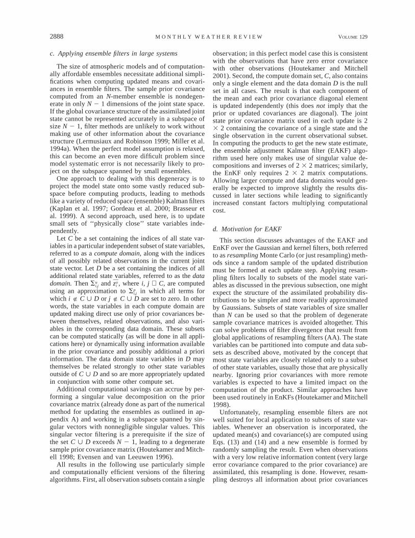
FIG. 1. Schematic showing results of applying different filters to two variables X1 and X2 in different computesubsets. (a) The prior distribution of an eight-member ensemble in the X1–X2 plane and the solid curve is an idealizeddistribution for an observation of X1. The results of applying (b) a kernel resampling filter, (c) a single Gaussianresampling filter, and (d) an ensemble adjustment Kalman filter are depicted in the same plane. The distribution foran ensemble Kalman filter would look similar to (d) with some amount of additional noise added to the ensemblepositions.

between state variables in different compute subsets.The assumption that the prior covariances between dif-ferent subsets are small is far from rigorous in appli-cations of interest, so it is inconvenient to lose all ofthis information every time observations become avail-able.

Figure 1a shows an idealized representation of a sys-tem with state variables X1 and X2 that are in differentcompute domains. An idealized observation of X1 withGaussian error distribution is indicated schematically bythe density plot along the X1 axis in Fig. 1a. Figure 1dshows the result of applying an EAKF in this case. Theadjustment pulls the value of X1 for all ensemble mem-bers toward the observed value. The covariance struc-ture between X1 and X2 is mostly preserved as the valuesof X2 are similarly pulled inward. The result is quali-tatively the same as applying a filter to X1 and X2 si-multaneously (no subsets). Figure 1c shows the resultsof applying a single Gaussian resampling filter and Fig.1b the result of a multiple kernel resampling filter as in

AA. The resampling filters destroy all prior informationabout the covariance of X1 and X2.

There are other related problems with resampling en-semble filters. First, it is impossible to meaningfullytrace individual assimilated ensemble trajectories intime. While the EAKF maintains the relative positionsof the prior samples, the letters in Figs. 1b and 1c arescrambled throughout the resulting distributions. Thiscan complicate diagnostic understanding of the assim-ilation. Trajectory tracing is easier in the EnKF than inthe resampling filters, but, especially with small ensem-bles, less straightforward than in the EAKF due to thenoise added in the perturbed observations.

Second, if only a single Gaussian kernel is being usedto compute the product, all information about higher-order moments of the prior distribution is destroyed eachtime data are assimilated (Fig. 1c). Anderson and An-derson (1999) introduced the sum of Gaussian kernelsapproximation to avoid this problem. In Fig. 1b, theprojection of higher-order structure on the individual


state variable axes is similar to that in Fig. 1d, but thedistribution itself winds up being qualitatively a quad-rupole because of the loss of covariance informationbetween X1 and X2.

These deficiencies of the resampling ensemble filtersoccur because a random sampling of the updated prob-ability distribution is used to generate the updated en-semble. In contrast, the EAKF and EnKF retain someinformation about prior covariances between state var-iables in separate compute subsets as shown schemat-ically in Fig. 1d for the EAKF (a figure for the EnKFwould be similar with some amount of additional noiseadded to the ensemble locations). For instance, obser-vations that have a relatively small information contentmake small changes to the prior distributions. Most ofthe covariance information between variables in differ-ent subsets survives the product step in this case. Thisis particularly relevant since the frequency of atmo-spheric and oceanic observations for problems of in-terest may lead to individual (subsets of ) observationsmaking relatively small adjustments to the prior distri-butions.

The EAKF and EnKF also preserve information abouthigher-order moments of prior probability distributionsas shown in Fig. 1d. Again, this information is partic-ularly valuable when observations make relatively smalladjustments to the prior distributions. For instance, ifthe dynamics of a model are generating distributionswith interesting higher moment structure, for instancea bimodality, this information can survive the updatestep using the EAKF or EnKF but is destroyed by re-sampling with a single Gaussian kernel.

Individual ensemble trajectories can be meaningfullytraced through time with the EAKF and the EnKF al-though the EnKF is noisier for small ensembles (seealso Figs. 3 and 9). If observations make small adjust-ments to the prior, individual ensemble members looksimilar to free runs of the model with periodic smalljumps where data are incorporated. Note that the EAKFis deterministic after initialization, requiring no gener-ation of random numbers once an initial ensemble iscreated.

The EAKF and EnKF are able to eliminate many ofthe shortcomings of the resampling filters. Unlike theresampling filters, they can be applied effectively whensubsets of state variables are used for computing up-dates. The EAKF and EnKF retain information abouthigher-order moments of prior distributions and indi-vidual ensemble trajectories are more physically rele-vant leading to easier diagnostic evaluation of assimi-lations. All of these advantages are particularly pro-nounced in instances where observations at any partic-ular time have a relatively small impact on the priordistribution, a situation that seems to be the case formost climate system model/data problems of interest.

e. Avoiding filter divergenceSince there are a number of approximations perme-

ating the EAKF and EnKF, there are naturally inaccu-

racies in the prior sample covariance and mean. As forother filter implementations, like the Kalman filter, sam-pling error or other approximations can cause the com-puted prior covariances to be too small at some times.The result is that less weight is given to new obser-vations when they become available resulting in in-creased error and further reduced covariance in the nextprior estimate. Eventually, the prior may no longer beimpacted significantly by the observations, and the as-similation will depart from the observations. A numberof sophisticated methods for dealing with this problemcan be developed. Here, only a simple remedy is used.The prior covariance matrix is multiplied by a constantfactor, usually slightly larger than one. If there are somelocal (in phase space) linear balances between the statevariables on the model’s attractor, then the applicationof small covariance inflation might be expected to main-tain these balances while still increasing uncertainty inthe state estimate. Clearly, even if there are locally linearbalanced aspects to the dynamics on the attractor, theapplication of sufficiently large covariance inflationswould lead to significantly unbalanced ensemble mem-bers.

The covariance inflation factor is selected empiricallyhere in order to give a filtering solution that does notdiverge from the observations while keeping the priorcovariances small. For all results shown, a search ofcovariance inflation values is made until a minimumvalue of ensemble mean rms error is found and resultsare only reported for these tuned cases. The impacts ofcovariance inflation in the EnKF are explored in Hamillet al. (2001). More sophisticated approaches to thisproblem are appropriate when dealing with models thathave significant systematic errors (i.e., when assimilat-ing real observations) and are currently being devel-oped.

f. ‘‘Distant’’ observations and maintaining priorcovariance

As pointed out in section 2d, one of the advantagesof the EAKF and EnKF is that they can maintain muchof the prior covariance structure even when applied in-dependently to small subsets of state variables. This isparticularly important in the applications reported herewhere each state variable is updated independently fromall others. If, however, two state variables that are close-ly related in the prior distribution are impacted by verydifferent subsets of observations, they may end up beingtoo weakly related in the updated distribution.

One possible (expensive) solution, would be to letevery state variable be impacted by all observations.This can, however, lead to another problem that has beennoted for the EnKF. Given a large number of obser-vations that are expected to be physically unrelated toa particular state variable, say because they are obser-vations of physically remote quantities, some of theseobservations will be highly correlated with the state


FIG. 2. Rms error as a function of forecast lead time (lead time 0is the error of the assimilation) for ensemble adjustment Kalman filterswith a 10-member ensemble (lowest dashed curve) and a 20-memberensemble (lowest solid curve) and for four-dimensional variationalassimilations that use the model as a strong constraint to fit obser-vations over a number of observing times. In generally descendingorder, the number of observation times used by the variational methodis two (dotted), 3 (dash–dotted), 4 (dashed), 5 (solid), 6 (dotted), 7(dash–dotted), 8 (dashed), 10 (solid), 12 (dotted), and 15 (dash–dot-ted).

variable by chance and will have an erroneous impacton the updated ensemble. The impact of spuriously cor-related remote observations can end up overwhelmingmore relevant observations (Hamill et al. 2001).

Following Houtekamer and Mitchell (2001), all low-order model results here multiply the covariances be-tween prior state variables and observation variables inthe joint state space by a correlation function with localsupport. The correlation function used is the same fifth-order piecewise rational function used by Gaspari andCohn [(1999), their equation (4.10)] and used in Hou-tekamer and Mitchell. This correlation function is char-acterized by a single parameter, c, that is the half-widthof the correlation function. The Schur product methodused in Houtekamer and Mitchell can be easily com-puted in the single state variable cases presented hereby simply multiplying the sample covariance betweenthe single observation and single state variable by thedistance dependent factor from the fifth-order rationalfunction.

3. Results from a low-order system

The EAKF and EnKF are applied to the 40-variablemodel of Lorenz [(1996), referred to hereafter as L96;see appendix B], which was used for simple tests oftargeted observation methodologies in Lorenz andEmanuel (1998). The number of state variables is greaterthan the smallest ensemble sizes (approximately 10) re-quired for usable sample statistics and the model has anumber of physical characteristics similar to those ofthe real atmosphere. All cases use synthetic observationsgenerated, as indicated in (4), over the course of a 1200time step segment of a very long control integration ofthe 40-variable model. Unless otherwise noted, resultsare presented from the 1000 step assimilation periodfrom step 200 to 1200 of this segment. Twenty-memberensembles are used unless otherwise noted.

For all L96 results reported, for both the EAKF andthe EnKF, a search is made through values of the co-variance inflation parameter and the correlation functionhalf-width, c. The covariance inflation parameter is in-dependently tuned for c’s of 0.05, 0.10, 0.15, 0.20, 0.25,0.30, and 0.35 in order to minimize the rms error overthe assimilation period. For the smallest c, state vari-ables are only impacted by observations at a distanceof less than 0.10 (total of 20% of the total domain widthof 1.0) while in the 0.35 case, the correlation functionactually wraps around in the cyclic domain allowingeven the most distant observations to have a nonnegli-gible impact on a state variable.

a. Identity observation operators

In the first case examined, the observational operator,h, is the identity (each state variable is observed di-rectly), the observational error covariance is diagonalwith all elements 4.0 (observations have independent

error variance of 4), and observations are available ev-ery time step. As discussed in detail in AA, the goal offiltering is to produce an ensemble with small ensemblemean error and with the true state being statisticallyindistinguishable from a randomly selected member ofthe ensemble. For the EAKF, the smallest time meanrms error of the ensemble mean for this assimilation is0.390 for a c of 0.3 and covariance inflation of 1.01.Figure 2 shows the rms error of the ensemble mean forthis assimilation and for forecasts started from the as-similation out to leads of 20 assimilation times for steps100–200 of the assimilation (101 forecasts; this periodis selected for comparison with four-dimensional vari-ational methods in section 5). Results for the EAKFwould be virtually indistinguishable if displayed forsteps 200–1200.

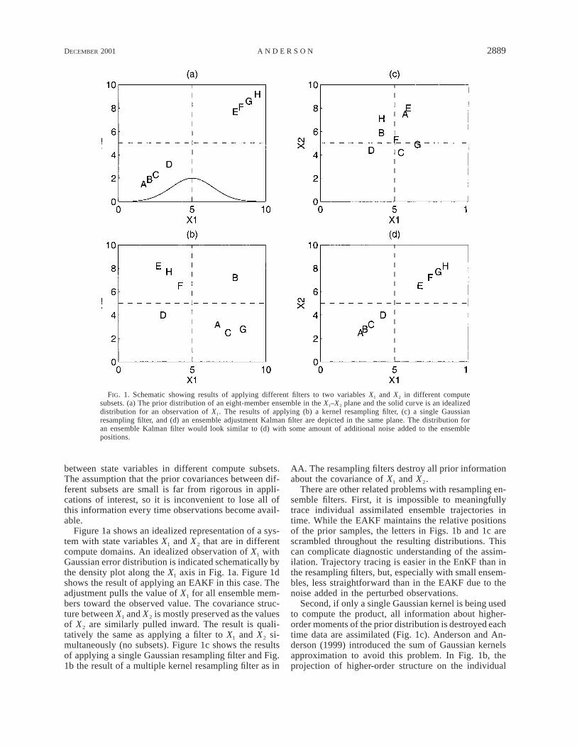
Figure 3a shows a time series of the ‘‘truth’’ fromthe control run and the corresponding ensemble mem-bers (the first 10 of the total of 20 are displayed to reduceclutter) and ensemble mean from the EAKF for variableX1. There is no evidence in this figure that the assimi-lation is inconsistent with the truth. The truth lies closeto the ensemble mean (compared to the range of thevariation in time) and generally is inside the 10 ensem-ble members plotted. The ensemble spread varies sig-nificantly in time; for instance, the ensemble is moreconfident about the state (less spread) when the wavetrough is approaching at assimilation time 885 than justafter the peak passes at time 875. The ability to traceindividual ensemble member trajectories in time is alsoclearly demonstrated; as noted in section 2 this could


FIG. 3. Time series of ‘‘truth’’ from long control run (solid gray),ensemble mean (thick dashed), and the first 10 of the 20 individualensemble members (thin dashed) for variable X1 of the L96 modelfrom assimilation times 850–900 using (a) an ensemble adjustmentKalman filter and (b) an ensemble Kalman filter.

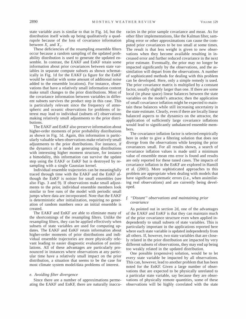
FIG. 4. Time series of rms error of ensemble mean from ensembleadjustment Kalman filter assimilation (dashed) and mean rms differ-ence between ensemble members and the ensemble mean (spread,solid) for variable X1 of the L96 model from assimilation times 850–900 of the same assimilation as in Fig. 3.

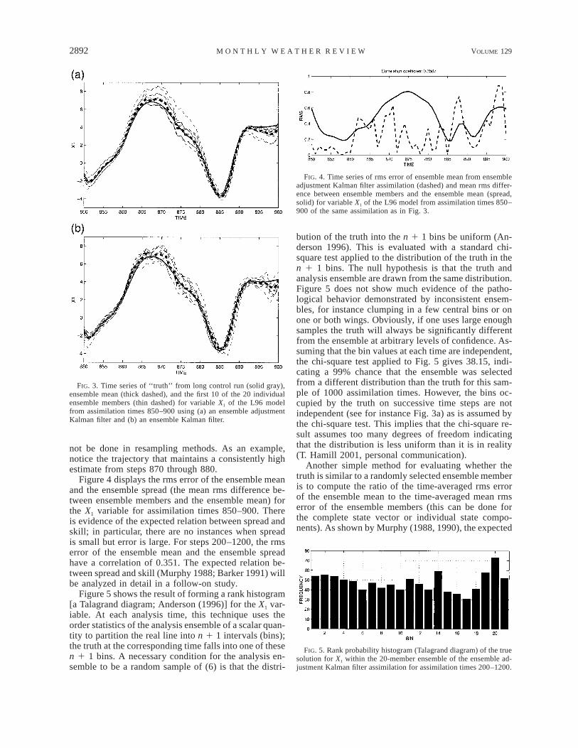
FIG. 5. Rank probability histogram (Talagrand diagram) of the truesolution for X1 within the 20-member ensemble of the ensemble ad-justment Kalman filter assimilation for assimilation times 200–1200.

not be done in resampling methods. As an example,notice the trajectory that maintains a consistently highestimate from steps 870 through 880.

Figure 4 displays the rms error of the ensemble meanand the ensemble spread (the mean rms difference be-tween ensemble members and the ensemble mean) forthe X1 variable for assimilation times 850–900. Thereis evidence of the expected relation between spread andskill; in particular, there are no instances when spreadis small but error is large. For steps 200–1200, the rmserror of the ensemble mean and the ensemble spreadhave a correlation of 0.351. The expected relation be-tween spread and skill (Murphy 1988; Barker 1991) willbe analyzed in detail in a follow-on study.

Figure 5 shows the result of forming a rank histogram[a Talagrand diagram; Anderson (1996)] for the X1 var-iable. At each analysis time, this technique uses theorder statistics of the analysis ensemble of a scalar quan-tity to partition the real line into n 1 1 intervals (bins);the truth at the corresponding time falls into one of thesen 1 1 bins. A necessary condition for the analysis en-semble to be a random sample of (6) is that the distri-

bution of the truth into the n 1 1 bins be uniform (An-derson 1996). This is evaluated with a standard chi-square test applied to the distribution of the truth in then 1 1 bins. The null hypothesis is that the truth andanalysis ensemble are drawn from the same distribution.Figure 5 does not show much evidence of the patho-logical behavior demonstrated by inconsistent ensem-bles, for instance clumping in a few central bins or onone or both wings. Obviously, if one uses large enoughsamples the truth will always be significantly differentfrom the ensemble at arbitrary levels of confidence. As-suming that the bin values at each time are independent,the chi-square test applied to Fig. 5 gives 38.15, indi-cating a 99% chance that the ensemble was selectedfrom a different distribution than the truth for this sam-ple of 1000 assimilation times. However, the bins oc-cupied by the truth on successive time steps are notindependent (see for instance Fig. 3a) as is assumed bythe chi-square test. This implies that the chi-square re-sult assumes too many degrees of freedom indicatingthat the distribution is less uniform than it is in reality(T. Hamill 2001, personal communication).

Another simple method for evaluating whether thetruth is similar to a randomly selected ensemble memberis to compute the ratio of the time-averaged rms errorof the ensemble mean to the time-averaged mean rmserror of the ensemble members (this can be done forthe complete state vector or individual state compo-nents). As shown by Murphy (1988, 1990), the expected


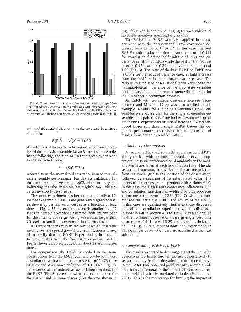
FIG. 6. Time mean of rms error of ensemble mean for steps 200–1200 for identity observation assimilations with observational errorvariances of 4.0 and 0.4 for 20-member EAKF and EnKF as a functionof correlation function half-width, c, for c ranging from 0.10 to 0.30.

value of this ratio (referred to as the rms ratio hereafter)should be

E(Ra) 5 Ï(N 1 1)/2N

if the truth is statistically indistinguishable from a mem-ber of the analysis ensemble for an N-member ensemble.In the following, the ratio of Ra for a given experimentto the expected value,

r 5 (Ra)/E(Ra),

referred to as the normalized rms ratio, is used to eval-uate ensemble performance. For this assimilation, r forthe complete state vector is 1.003, close to unity butindicating that the ensemble has slightly too little un-certainty (too little spread).

The same experiment has been run using only a 10-member ensemble. Results are generally slightly worse,as shown by the rms error curves as a function of leadtime in Fig. 2. Using ensembles much smaller than 10leads to sample covariance estimates that are too poorfor the filter to converge. Using ensembles larger than20 leads to small improvements in the rms errors.

It is important to examine the rate at which ensemblemean error and spread grow if the assimilation is turnedoff to verify that the EAKF is performing in a usefulfashion. In this case, the forecast error growth plot inFig. 2 shows that error doubles in about 12 assimilationtimes.

For comparison, the EnKF is applied to the sameobservations from the L96 model and produces its bestassimilation with a time mean rms error of 0.476 for cof 0.25 and covariance inflation of 1.12 (see Fig. 6).Time series of the individual assimilation members forthe EnKF (Fig. 3b) are somewhat noisier than those forthe EAKF and in some places (like the one shown in

Fig. 3b) it can become challenging to trace individualensemble members meaningfully in time.

The EAKF and EnKF were also applied in an ex-periment with the observational error covariance de-creased by a factor of 10 to 0.4. In this case, the bestEAKF result produced a time mean rms error of 0.144for correlation function half-width c of 0.30 and co-variance inflation of 1.015 while the best EnKF had rmserror of 0.171 for c of 0.20 and covariance inflation of1.06 (Fig. 6). The ratio of the best EAKF to EnKF rmsis 0.842 for the reduced variance case, a slight increasefrom the 0.819 ratio in the larger variance case. Theratio of this reduced observational error variance to the‘‘climatological’’ variance of the L96 state variablescould be argued to be more consistent with the ratio forthe atmospheric prediction problem.

An EnKF with two independent ensemble sets (Hou-tekamer and Mitchell 1998) was also applied to thisexample. Results for a pair of 10-member EnKF en-sembles were worse than for the single 20-member en-semble. This paired EnKF method was evaluated for allother EnKF experiments discussed here and always pro-duced larger rms than a single EnKF. Given this de-graded performance, there is no further discussion ofresults from paired ensemble EnKFs.

b. Nonlinear observations

A second test in the L96 model appraises the EAKF’sability to deal with nonlinear forward observation op-erators. Forty observations placed randomly in the mod-el domain are taken at each assimilation time. The ob-servational operator, h, involves a linear interpolationfrom the model grid to the location of the observation,followed by a squaring of the interpolated value. Theobservational errors are independent with variance 64.0.In this case, the EAKF with covariance inflation of 1.02and correlation function half-width c of 0.30 producesa time mean rms error of 0.338 (Fig. 7) while the nor-malized rms ratio r is 1.002. The results of the EAKFin this case are qualitatively similar to those discussedin a related assimilation experiment, which is discussedin more detail in section 4. The EnKF was also appliedin this nonlinear observations case giving a best timemean rms of 0.421 for c of 0.25 and covariance inflationof 1.12 (Fig. 7). A number of additional experiments inthis nonlinear observation case are examined in the nextsubsection.

c. Comparison of EAKF and EnKF

The results presented to date suggest that the inclusionof noise in the EnKF through the use of perturbed ob-servations may lead to degraded performance relativeto the EAKF. One potential problem with ensemble Kal-man filters in general is the impact of spurious corre-lations with physically unrelated variables (Hamill et al.2001). This is the motivation for limiting the impact of


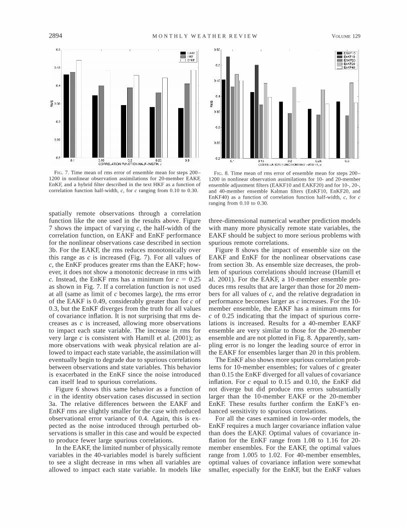
FIG. 7. Time mean of rms error of ensemble mean for steps 200–1200 in nonlinear observation assimilations for 20-member EAKF,EnKF, and a hybrid filter described in the text HKF as a function ofcorrelation function half-width, c, for c ranging from 0.10 to 0.30.

FIG. 8. Time mean of rms error of ensemble mean for steps 200–1200 in nonlinear observation assimilations for 10- and 20-memberensemble adjustment filters (EAKF10 and EAKF20) and for 10-, 20-,and 40-member ensemble Kalman filters (EnKF10, EnKF20, andEnKF40) as a function of correlation function half-width, c, for cranging from 0.10 to 0.30.

spatially remote observations through a correlationfunction like the one used in the results above. Figure7 shows the impact of varying c, the half-width of thecorrelation function, on EAKF and EnKF performancefor the nonlinear observations case described in section3b. For the EAKF, the rms reduces monotonically overthis range as c is increased (Fig. 7). For all values ofc, the EnKF produces greater rms than the EAKF; how-ever, it does not show a monotonic decrease in rms withc. Instead, the EnKF rms has a minimum for c 5 0.25as shown in Fig. 7. If a correlation function is not usedat all (same as limit of c becomes large), the rms errorof the EAKF is 0.49, considerably greater than for c of0.3, but the EnKF diverges from the truth for all valuesof covariance inflation. It is not surprising that rms de-creases as c is increased, allowing more observationsto impact each state variable. The increase in rms forvery large c is consistent with Hamill et al. (2001); asmore observations with weak physical relation are al-lowed to impact each state variable, the assimilation willeventually begin to degrade due to spurious correlationsbetween observations and state variables. This behavioris exacerbated in the EnKF since the noise introducedcan itself lead to spurious correlations.

Figure 6 shows this same behavior as a function ofc in the identity observation cases discussed in section3a. The relative differences between the EAKF andEnKF rms are slightly smaller for the case with reducedobservational error variance of 0.4. Again, this is ex-pected as the noise introduced through perturbed ob-servations is smaller in this case and would be expectedto produce fewer large spurious correlations.

In the EAKF, the limited number of physically remotevariables in the 40-variables model is barely sufficientto see a slight decrease in rms when all variables areallowed to impact each state variable. In models like

three-dimensional numerical weather prediction modelswith many more physically remote state variables, theEAKF should be subject to more serious problems withspurious remote correlations.

Figure 8 shows the impact of ensemble size on theEAKF and EnKF for the nonlinear observations casefrom section 3b. As ensemble size decreases, the prob-lem of spurious correlations should increase (Hamill etal. 2001). For the EAKF, a 10-member ensemble pro-duces rms results that are larger than those for 20 mem-bers for all values of c, and the relative degradation inperformance becomes larger as c increases. For the 10-member ensemble, the EAKF has a minimum rms forc of 0.25 indicating that the impact of spurious corre-lations is increased. Results for a 40-member EAKFensemble are very similar to those for the 20-memberensemble and are not plotted in Fig. 8. Apparently, sam-pling error is no longer the leading source of error inthe EAKF for ensembles larger than 20 in this problem.

The EnKF also shows more spurious correlation prob-lems for 10-member ensembles; for values of c greaterthan 0.15 the EnKF diverged for all values of covarianceinflation. For c equal to 0.15 and 0.10, the EnKF didnot diverge but did produce rms errors substantiallylarger than the 10-member EAKF or the 20-memberEnKF. These results further confirm the EnKF’s en-hanced sensitivity to spurious correlations.

For all the cases examined in low-order models, theEnKF requires a much larger covariance inflation valuethan does the EAKF. Optimal values of covariance in-flation for the EnKF range from 1.08 to 1.16 for 20-member ensembles. For the EAKF, the optimal valuesrange from 1.005 to 1.02. For 40-member ensembles,optimal values of covariance inflation were somewhatsmaller, especially for the EnKF, but the EnKF values


were still much larger than those for the EAKF. Thelarger values of covariance inflation are required be-cause the EnKF has an extra source of potential filterdivergence since only the expected value of the updatedsample covariance is equal to that given by (13). Bychance, there will be cases when the updated covarianceis smaller than the expected value. In general, this isexpected to lead to a prior estimate with reduced co-variance and increased error at the next assimilationtime, which in turn is expected to lead to an even morereduced estimate after the next assimilation. Turning upcovariance inflation to avoid filter divergence at suchtimes leads to the observational data being given toomuch weight at other times when the updated covarianceestimates are too large by chance. The net result is anexpected degradation of EnKF performance.

To further elucidate the differences between theEAKF and EnKF, a hybrid filter (referred to as HKFhereafter) was applied to the nonlinear observation case.The hybrid filter begins by applying the EnKF to a statevariable–observation pair. The resulting updated ensem-ble of the state variable has variance whose expectedvalue is given by (13), but whose actual sample variancediffers from this value due to the use of perturbed ob-servations. As a second step, the hybrid filter scales theensemble around its mean so that the resulting ensemblehas both the same mean and sample variance as theEAKF. However, the noise introduced by the perturbedobservations can still impact higher-order moments ofthe state variable distribution and its covariance withother state variables. Figure 7 shows results for theEAKF, HKF, and EnKF for a range of correlation func-tion c’s. In all cases, the rms of the HKF is between theEAKF and EnKF values, but the HKF rms is muchcloser to the EAKF for small values of c. As anticipated,the values of covariance inflation required for the bestrms for the HKF are smaller than for the EnKF, withvalues ranging from 1.01 for c of 0.10 to 1.04 for c of0.20, 0.25, and 0.30. The HKF experiment can beviewed as isolating the impacts of enhanced spuriouscorrelations from the impacts of the larger covarianceinflation required to avoid filter divergence in the EnKF.For small c, almost all the difference between the EnKFand EAKF is due to the enhanced covariance inflationwhile for larger c, most of the degraded performance isdue to enhanced impact of spurious correlations.

The EnKF’s addition of random noise through ‘‘per-turbed observations’’ at each assimilation step appearsto be sufficient to degrade the quality of the assimilationthrough these two mechanisms. The L96 system is quitetolerant of added noise with off-attractor perturbationsdecaying relatively quickly and nearly uniformly towardthe attractor; the noise added in the EnKF could be ofadditional concern in less tolerant systems.

4. Estimation of model parametersMost atmospheric models have many parameters (in

dynamics and subgrid-scale physical parameterizations)

for which appropriate values are not known precisely.One can recast these parameters as independent modelvariables (Derber 1989), and use assimilation to estimatevalues for the unknown parameters. Ensemble filters canproduce a sample of the probability distribution of suchparameters given available observations.

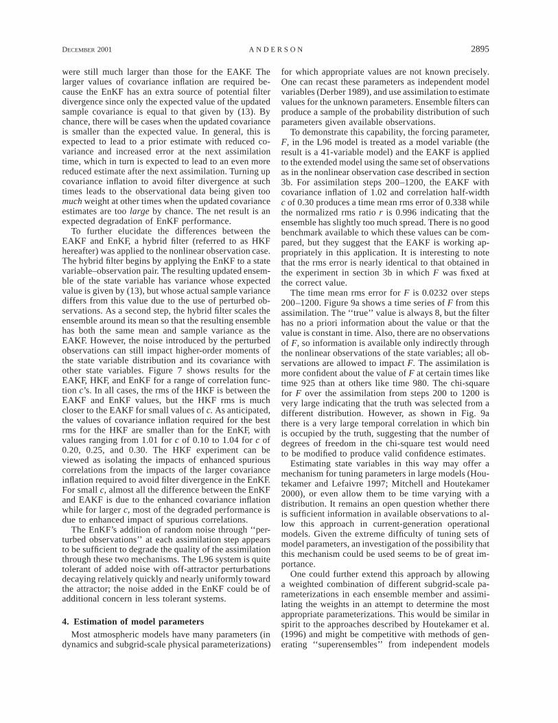
To demonstrate this capability, the forcing parameter,F, in the L96 model is treated as a model variable (theresult is a 41-variable model) and the EAKF is appliedto the extended model using the same set of observationsas in the nonlinear observation case described in section3b. For assimilation steps 200–1200, the EAKF withcovariance inflation of 1.02 and correlation half-widthc of 0.30 produces a time mean rms error of 0.338 whilethe normalized rms ratio r is 0.996 indicating that theensemble has slightly too much spread. There is no goodbenchmark available to which these values can be com-pared, but they suggest that the EAKF is working ap-propriately in this application. It is interesting to notethat the rms error is nearly identical to that obtained inthe experiment in section 3b in which F was fixed atthe correct value.

The time mean rms error for F is 0.0232 over steps200–1200. Figure 9a shows a time series of F from thisassimilation. The ‘‘true’’ value is always 8, but the filterhas no a priori information about the value or that thevalue is constant in time. Also, there are no observationsof F, so information is available only indirectly throughthe nonlinear observations of the state variables; all ob-servations are allowed to impact F. The assimilation ismore confident about the value of F at certain times liketime 925 than at others like time 980. The chi-squarefor F over the assimilation from steps 200 to 1200 isvery large indicating that the truth was selected from adifferent distribution. However, as shown in Fig. 9athere is a very large temporal correlation in which binis occupied by the truth, suggesting that the number ofdegrees of freedom in the chi-square test would needto be modified to produce valid confidence estimates.

Estimating state variables in this way may offer amechanism for tuning parameters in large models (Hou-tekamer and Lefaivre 1997; Mitchell and Houtekamer2000), or even allow them to be time varying with adistribution. It remains an open question whether thereis sufficient information in available observations to al-low this approach in current-generation operationalmodels. Given the extreme difficulty of tuning sets ofmodel parameters, an investigation of the possibility thatthis mechanism could be used seems to be of great im-portance.

One could further extend this approach by allowinga weighted combination of different subgrid-scale pa-rameterizations in each ensemble member and assimi-lating the weights in an attempt to determine the mostappropriate parameterizations. This would be similar inspirit to the approaches described by Houtekamer et al.(1996) and might be competitive with methods of gen-erating ‘‘superensembles’’ from independent models


FIG. 9. Time series of truth from long control run (solid gray),ensemble mean (thick dashed) and the first 10 of the 20 individualensemble members (thin dashed) for the model forcing variable, F,of the L96 model from assimilation times 900–1000 for an assimi-lation with nonlinear observations operator described in text; resultsfrom (a) an ensemble adjustment Kalman filter and (b) an ensembleKalman filter.

(Goerss 2000; Harrison et al. 1999; Evans et al. 2000;Krishnamurthi et al. 1999; Ziehmann 2000; Richardson2000).

The best EnKF result for this problem had an rmserror of 0.417 for c of 0.20 and covariance inflation1.08. However, the rms error in F is 0.108, about fourtimes as large as for the EAKF. Figure 9b shows a timeseries of the EnKF estimate of the forcing variable, F,for comparison with Fig. 9a. The spread and rms errorare much larger and the individual EnKF trajectoriesdisplay a much greater high-frequency time variationthan did those for the EAKF.

The introduction of noise in the EnKF is particularlyproblematic for the assimilation of F because, in gen-eral, all available observations are expected to be weak-ly, but equally, correlated with F. There is no naturalway to use a correlation function to allow only somesubset of observations to impact F as there was for statevariables. The result is that the EnKF’s tendency to beadversely impacted by spurious correlations with weak-ly related observations has a much greater impact than

for regular state variables. This result suggests that theEnKF will have particular difficulty in other cases wherea large number of weakly correlated observations areavailable for a given state variable, for instance certainkinds of wide field of view satellite observations.

5. Comparison to four-dimensional variationalassimilation

Four-dimensional variational assimilation methods(4DVAR) are generally regarded as the present state ofthe art for the atmosphere and ocean (Tziperman andSirkes 1997). A 4DVAR has been applied to the L96model and results compared to those for the EAKF. The4DVAR uses the L96 model as a strong constraint (Zu-panski 1997), perhaps not much of an issue in a perfectmodel assimilation. The 4DVAR optimization is per-formed with an explicit finite-difference computation ofthe derivative, with 128-bit floating point arithmetic,and uses as many iterations of a preconditioned, limited-memory quasi-Newton conjugate gradient algorithm(NAG subroutine E04DGF) as are required to convergeto machine precision (in practice the number of itera-tions is generally less than 200). The observations avail-able to the 4DVAR are identical to those used by theEAKF, and the number of observation times being fitby the 4DVAR is varied from 2 to 15 (cases above 15began to present problems for the optimization evenwith 128 bits).

Figure 2 compares the rms error of the 4DVAR as-similations and forecasts to those for the EAKF assim-ilations out to leads of 20 assimilation times for the firstcase presented in section 3. All results are the mean for101 separate assimilations and subsequent forecasts, be-tween assimilation steps 100–200. As the number ofobservation times used in the 4DVAR is increased, erroris reduced but always remains much greater than theEAKF error. The 4DVAR cases also show acceleratederror growth as a function of forecast lead compared tothe EAKF when the number of observation times forthe 4DVAR gets large, a symptom of increasing over-fitting of the observations (Swanson et al. 1998). AnEAKF with only 10 ensemble members is still able tooutperform all of the 4DVAR assimilations (Fig. 2).

The EAKF outperforms 4DVAR by using more com-plete information about the distribution of the prior. Inaddition to providing better estimates of the state, theEAKF also provides information about the uncertaintyin this estimate through the ensemble as discussed insection 3. Note that recent work by Hansen and Smith(2001) suggests that combining the capabilities of4DVAR and ensemble filters may lead to a hybrid thatis superior to either. Other enhancements to the 4DVARalgorithm could also greatly enhance its performance.Still, these results suggest that the EAKF should beseriously considered as an alternative to 4DVAR al-gorithms in a variety of applications.


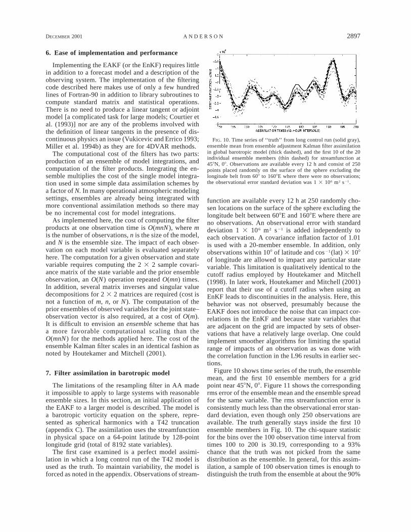
FIG. 10. Time series of ‘‘truth’’ from long control run (solid gray),ensemble mean from ensemble adjustment Kalman filter assimilationin global barotropic model (thick dashed), and the first 10 of the 20individual ensemble members (thin dashed) for streamfunction at458N, 08. Observations are available every 12 h and consist of 250points placed randomly on the surface of the sphere excluding thelongitude belt from 608 to 1608E where there were no observations;the observational error standard deviation was 1 3 106 m2 s21.

6. Ease of implementation and performance

Implementing the EAKF (or the EnKF) requires littlein addition to a forecast model and a description of theobserving system. The implementation of the filteringcode described here makes use of only a few hundredlines of Fortran-90 in addition to library subroutines tocompute standard matrix and statistical operations.There is no need to produce a linear tangent or adjointmodel [a complicated task for large models; Courtier etal. (1993)] nor are any of the problems involved withthe definition of linear tangents in the presence of dis-continuous physics an issue (Vukicevic and Errico 1993;Miller et al. 1994b) as they are for 4DVAR methods.

The computational cost of the filters has two parts:production of an ensemble of model integrations, andcomputation of the filter products. Integrating the en-semble multiplies the cost of the single model integra-tion used in some simple data assimilation schemes bya factor of N. In many operational atmospheric modelingsettings, ensembles are already being integrated withmore conventional assimilation methods so there maybe no incremental cost for model integrations.

As implemented here, the cost of computing the filterproducts at one observation time is O(mnN), where mis the number of observations, n is the size of the model,and N is the ensemble size. The impact of each obser-vation on each model variable is evaluated separatelyhere. The computation for a given observation and statevariable requires computing the 2 3 2 sample covari-ance matrix of the state variable and the prior ensembleobservation, an O(N) operation repeated O(mn) times.In addition, several matrix inverses and singular valuedecompositions for 2 3 2 matrices are required (cost isnot a function of m, n, or N). The computation of theprior ensembles of observed variables for the joint state–observation vector is also required, at a cost of O(m).It is difficult to envision an ensemble scheme that hasa more favorable computational scaling than theO(mnN) for the methods applied here. The cost of theensemble Kalman filter scales in an identical fashion asnoted by Houtekamer and Mitchell (2001).

7. Filter assimilation in barotropic model

The limitations of the resampling filter in AA madeit impossible to apply to large systems with reasonableensemble sizes. In this section, an initial application ofthe EAKF to a larger model is described. The model isa barotropic vorticity equation on the sphere, repre-sented as spherical harmonics with a T42 truncation(appendix C). The assimilation uses the streamfunctionin physical space on a 64-point latitude by 128-pointlongitude grid (total of 8192 state variables).

The first case examined is a perfect model assimi-lation in which a long control run of the T42 model isused as the truth. To maintain variability, the model isforced as noted in the appendix. Observations of stream-

function are available every 12 h at 250 randomly cho-sen locations on the surface of the sphere excluding thelongitude belt between 608E and 1608E where there areno observations. An observational error with standarddeviation 1 3 106 m2 s21 is added independently toeach observation. A covariance inflation factor of 1.01is used with a 20-member ensemble. In addition, onlyobservations within 108 of latitude and cos21(lat) 3 108of longitude are allowed to impact any particular statevariable. This limitation is qualitatively identical to thecutoff radius employed by Houtekamer and Mitchell(1998). In later work, Houtekamer and Mitchell (2001)report that their use of a cutoff radius when using anEnKF leads to discontinuities in the analysis. Here, thisbehavior was not observed, presumably because theEAKF does not introduce the noise that can impact cor-relations in the EnKF and because state variables thatare adjacent on the grid are impacted by sets of obser-vations that have a relatively large overlap. One couldimplement smoother algorithms for limiting the spatialrange of impacts of an observation as was done withthe correlation function in the L96 results in earlier sec-tions.

Figure 10 shows time series of the truth, the ensemblemean, and the first 10 ensemble members for a gridpoint near 458N, 08. Figure 11 shows the correspondingrms error of the ensemble mean and the ensemble spreadfor the same variable. The rms streamfunction error isconsistently much less than the observational error stan-dard deviation, even though only 250 observations areavailable. The truth generally stays inside the first 10ensemble members in Fig. 10. The chi-square statisticfor the bins over the 100 observation time interval fromtimes 100 to 200 is 30.19, corresponding to a 93%chance that the truth was not picked from the samedistribution as the ensemble. In general, for this assim-ilation, a sample of 100 observation times is enough todistinguish the truth from the ensemble at about the 90%


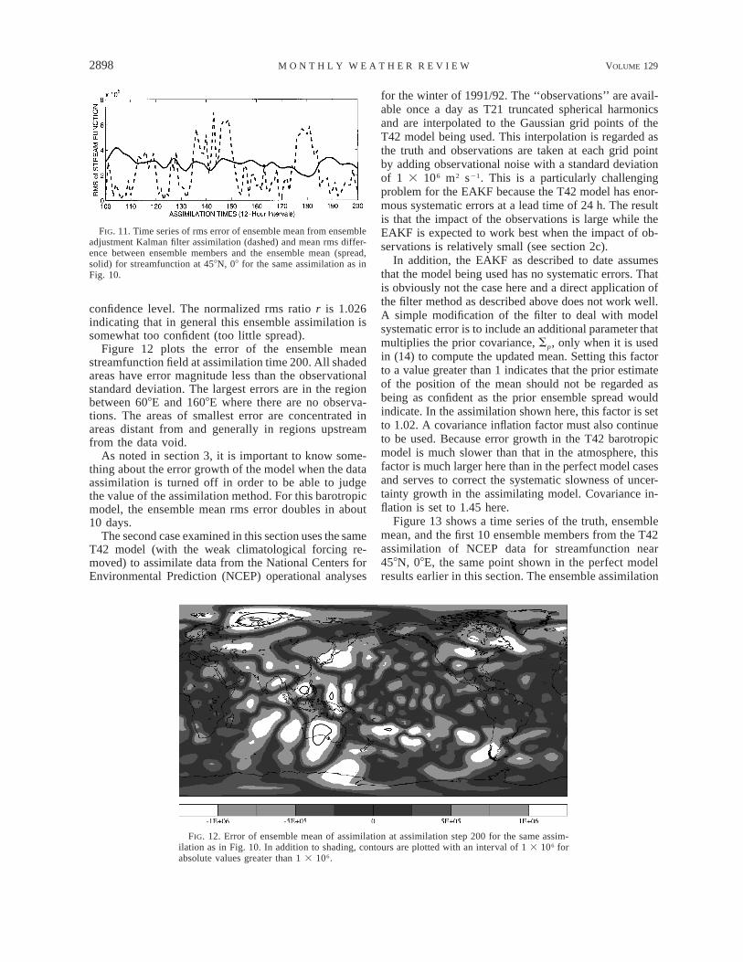
FIG. 11. Time series of rms error of ensemble mean from ensembleadjustment Kalman filter assimilation (dashed) and mean rms differ-ence between ensemble members and the ensemble mean (spread,solid) for streamfunction at 458N, 08 for the same assimilation as inFig. 10.

FIG. 12. Error of ensemble mean of assimilation at assimilation step 200 for the same assim-ilation as in Fig. 10. In addition to shading, contours are plotted with an interval of 1 3 106 forabsolute values greater than 1 3 106.

confidence level. The normalized rms ratio r is 1.026indicating that in general this ensemble assimilation issomewhat too confident (too little spread).

Figure 12 plots the error of the ensemble meanstreamfunction field at assimilation time 200. All shadedareas have error magnitude less than the observationalstandard deviation. The largest errors are in the regionbetween 608E and 1608E where there are no observa-tions. The areas of smallest error are concentrated inareas distant from and generally in regions upstreamfrom the data void.

As noted in section 3, it is important to know some-thing about the error growth of the model when the dataassimilation is turned off in order to be able to judgethe value of the assimilation method. For this barotropicmodel, the ensemble mean rms error doubles in about10 days.

The second case examined in this section uses the sameT42 model (with the weak climatological forcing re-moved) to assimilate data from the National Centers forEnvironmental Prediction (NCEP) operational analyses

for the winter of 1991/92. The ‘‘observations’’ are avail-able once a day as T21 truncated spherical harmonicsand are interpolated to the Gaussian grid points of theT42 model being used. This interpolation is regarded asthe truth and observations are taken at each grid pointby adding observational noise with a standard deviationof 1 3 106 m2 s21. This is a particularly challengingproblem for the EAKF because the T42 model has enor-mous systematic errors at a lead time of 24 h. The resultis that the impact of the observations is large while theEAKF is expected to work best when the impact of ob-servations is relatively small (see section 2c).

In addition, the EAKF as described to date assumesthat the model being used has no systematic errors. Thatis obviously not the case here and a direct application ofthe filter method as described above does not work well.A simple modification of the filter to deal with modelsystematic error is to include an additional parameter thatmultiplies the prior covariance, Sp, only when it is usedin (14) to compute the updated mean. Setting this factorto a value greater than 1 indicates that the prior estimateof the position of the mean should not be regarded asbeing as confident as the prior ensemble spread wouldindicate. In the assimilation shown here, this factor is setto 1.02. A covariance inflation factor must also continueto be used. Because error growth in the T42 barotropicmodel is much slower than that in the atmosphere, thisfactor is much larger here than in the perfect model casesand serves to correct the systematic slowness of uncer-tainty growth in the assimilating model. Covariance in-flation is set to 1.45 here.

Figure 13 shows a time series of the truth, ensemblemean, and the first 10 ensemble members from the T42assimilation of NCEP data for streamfunction near458N, 08E, the same point shown in the perfect modelresults earlier in this section. The ensemble assimilation


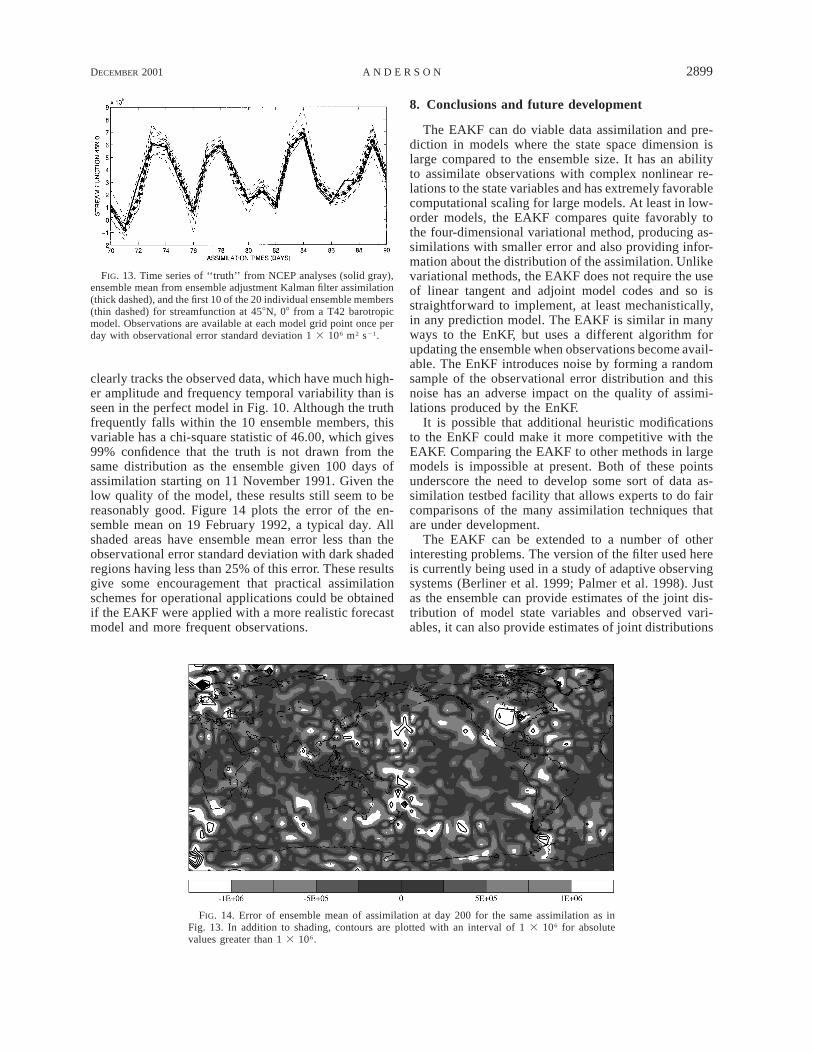
FIG. 13. Time series of ‘‘truth’’ from NCEP analyses (solid gray),ensemble mean from ensemble adjustment Kalman filter assimilation(thick dashed), and the first 10 of the 20 individual ensemble members(thin dashed) for streamfunction at 458N, 08 from a T42 barotropicmodel. Observations are available at each model grid point once perday with observational error standard deviation 1 3 106 m2 s21.

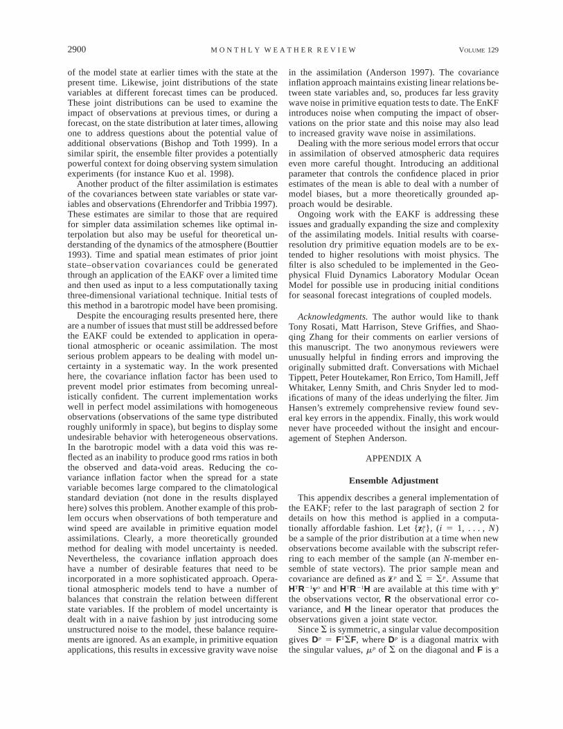
FIG. 14. Error of ensemble mean of assimilation at day 200 for the same assimilation as inFig. 13. In addition to shading, contours are plotted with an interval of 1 3 106 for absolutevalues greater than 1 3 106.

clearly tracks the observed data, which have much high-er amplitude and frequency temporal variability than isseen in the perfect model in Fig. 10. Although the truthfrequently falls within the 10 ensemble members, thisvariable has a chi-square statistic of 46.00, which gives99% confidence that the truth is not drawn from thesame distribution as the ensemble given 100 days ofassimilation starting on 11 November 1991. Given thelow quality of the model, these results still seem to bereasonably good. Figure 14 plots the error of the en-semble mean on 19 February 1992, a typical day. Allshaded areas have ensemble mean error less than theobservational error standard deviation with dark shadedregions having less than 25% of this error. These resultsgive some encouragement that practical assimilationschemes for operational applications could be obtainedif the EAKF were applied with a more realistic forecastmodel and more frequent observations.

8. Conclusions and future development

The EAKF can do viable data assimilation and pre-diction in models where the state space dimension islarge compared to the ensemble size. It has an abilityto assimilate observations with complex nonlinear re-lations to the state variables and has extremely favorablecomputational scaling for large models. At least in low-order models, the EAKF compares quite favorably tothe four-dimensional variational method, producing as-similations with smaller error and also providing infor-mation about the distribution of the assimilation. Unlikevariational methods, the EAKF does not require the useof linear tangent and adjoint model codes and so isstraightforward to implement, at least mechanistically,in any prediction model. The EAKF is similar in manyways to the EnKF, but uses a different algorithm forupdating the ensemble when observations become avail-able. The EnKF introduces noise by forming a randomsample of the observational error distribution and thisnoise has an adverse impact on the quality of assimi-lations produced by the EnKF.

It is possible that additional heuristic modificationsto the EnKF could make it more competitive with theEAKF. Comparing the EAKF to other methods in largemodels is impossible at present. Both of these pointsunderscore the need to develop some sort of data as-similation testbed facility that allows experts to do faircomparisons of the many assimilation techniques thatare under development.

The EAKF can be extended to a number of otherinteresting problems. The version of the filter used hereis currently being used in a study of adaptive observingsystems (Berliner et al. 1999; Palmer et al. 1998). Justas the ensemble can provide estimates of the joint dis-tribution of model state variables and observed vari-ables, it can also provide estimates of joint distributions


of the model state at earlier times with the state at thepresent time. Likewise, joint distributions of the statevariables at different forecast times can be produced.These joint distributions can be used to examine theimpact of observations at previous times, or during aforecast, on the state distribution at later times, allowingone to address questions about the potential value ofadditional observations (Bishop and Toth 1999). In asimilar spirit, the ensemble filter provides a potentiallypowerful context for doing observing system simulationexperiments (for instance Kuo et al. 1998).

Another product of the filter assimilation is estimatesof the covariances between state variables or state var-iables and observations (Ehrendorfer and Tribbia 1997).These estimates are similar to those that are requiredfor simpler data assimilation schemes like optimal in-terpolation but also may be useful for theoretical un-derstanding of the dynamics of the atmosphere (Bouttier1993). Time and spatial mean estimates of prior jointstate–observation covariances could be generatedthrough an application of the EAKF over a limited timeand then used as input to a less computationally taxingthree-dimensional variational technique. Initial tests ofthis method in a barotropic model have been promising.

Despite the encouraging results presented here, thereare a number of issues that must still be addressed beforethe EAKF could be extended to application in opera-tional atmospheric or oceanic assimilation. The mostserious problem appears to be dealing with model un-certainty in a systematic way. In the work presentedhere, the covariance inflation factor has been used toprevent model prior estimates from becoming unreal-istically confident. The current implementation workswell in perfect model assimilations with homogeneousobservations (observations of the same type distributedroughly uniformly in space), but begins to display someundesirable behavior with heterogeneous observations.In the barotropic model with a data void this was re-flected as an inability to produce good rms ratios in boththe observed and data-void areas. Reducing the co-variance inflation factor when the spread for a statevariable becomes large compared to the climatologicalstandard deviation (not done in the results displayedhere) solves this problem. Another example of this prob-lem occurs when observations of both temperature andwind speed are available in primitive equation modelassimilations. Clearly, a more theoretically groundedmethod for dealing with model uncertainty is needed.Nevertheless, the covariance inflation approach doeshave a number of desirable features that need to beincorporated in a more sophisticated approach. Opera-tional atmospheric models tend to have a number ofbalances that constrain the relation between differentstate variables. If the problem of model uncertainty isdealt with in a naive fashion by just introducing someunstructured noise to the model, these balance require-ments are ignored. As an example, in primitive equationapplications, this results in excessive gravity wave noise

in the assimilation (Anderson 1997). The covarianceinflation approach maintains existing linear relations be-tween state variables and, so, produces far less gravitywave noise in primitive equation tests to date. The EnKFintroduces noise when computing the impact of obser-vations on the prior state and this noise may also leadto increased gravity wave noise in assimilations.

Dealing with the more serious model errors that occurin assimilation of observed atmospheric data requireseven more careful thought. Introducing an additionalparameter that controls the confidence placed in priorestimates of the mean is able to deal with a number ofmodel biases, but a more theoretically grounded ap-proach would be desirable.

Ongoing work with the EAKF is addressing theseissues and gradually expanding the size and complexityof the assimilating models. Initial results with coarse-resolution dry primitive equation models are to be ex-tended to higher resolutions with moist physics. Thefilter is also scheduled to be implemented in the Geo-physical Fluid Dynamics Laboratory Modular OceanModel for possible use in producing initial conditionsfor seasonal forecast integrations of coupled models.

Acknowledgments. The author would like to thankTony Rosati, Matt Harrison, Steve Griffies, and Shao-qing Zhang for their comments on earlier versions ofthis manuscript. The two anonymous reviewers wereunusually helpful in finding errors and improving theoriginally submitted draft. Conversations with MichaelTippett, Peter Houtekamer, Ron Errico, Tom Hamill, JeffWhitaker, Lenny Smith, and Chris Snyder led to mod-ifications of many of the ideas underlying the filter. JimHansen’s extremely comprehensive review found sev-eral key errors in the appendix. Finally, this work wouldnever have proceeded without the insight and encour-agement of Stephen Anderson.

APPENDIX A

Ensemble Adjustment

This appendix describes a general implementation ofthe EAKF; refer to the last paragraph of section 2 fordetails on how this method is applied in a computa-tionally affordable fashion. Let { }, (i 5 1, . . . , N)pzi

be a sample of the prior distribution at a time when newobservations become available with the subscript refer-ring to each member of the sample (an N-member en-semble of state vectors). The prior sample mean andcovariance are defined as p and S 5 Sp. Assume thatzHTR21yo and HTR21H are available at this time with yo

the observations vector, R the observational error co-variance, and H the linear operator that produces theobservations given a joint state vector.

Since S is symmetric, a singular value decompositiongives Dp 5 FTSF, where Dp is a diagonal matrix withthe singular values, mp of S on the diagonal and F is a


unitary matrix (FTF 5 I, F21 5 FT, (FT)21 5 F). Ap-plying FT and F in this fashion is a rotation of S to areference frame in which the prior sample covarianceis diagonal.

Next, one can apply a scaling in this rotated framein order to make the prior sample covariance the iden-tity. The matrix (GT)21FTSFG21, where G is a diagonalmatrix with the square root of the singular values, mp,on the diagonal, is the identity matrix, I.

Next, a singular value decomposition can be per-formed on the matrix GTFTHTR21HFG; this is a rotationto a reference frame in which the scaled inverse obser-

vational ‘‘covariance’’ matrix, HTR21H, is a diagonalmatrix, D 5 UTGTFTHTR21HFGU, with the diagonal el-ements the singular values, m. The prior covariance canalso be moved to this reference frame, and it is still theidentity since U is unitary, I 5 UT(GT)21FTSFG21U.

The updated covariance can be computed easily inthis reference frame since the prior covariance inverseis just I and the observed covariance inverse is diagonal.The updated covariance can then be moved back to theoriginal reference frame by unrotating, unscaling, andunrotating. (Note that G is symmetric.)

More formally, the updated covariance can be eval-uated as

u 21 21 21 21 21 21 21T 21 T T T T T T T 21 21 21 21S 5 (S 1 H R H) 5 (F ) G (U ) [U (G ) F (S 1 H R H) FG U]U GF21 21 21 21 21 21T T T 21 21 T 21 T T T 21 215 (F ) G (U ) {[U GF (S 1 H R H)(F ) G (U ) ] }U GF21 21 21 21 21 21 21 21T T T 21 21 T T T 21 21 T 21 T T T 21 215 (F ) G (U ) {[U GF S (F ) G (U ) 1 U GF H R H(F ) G (U ) ] }U GF21 21 21 21 21T T T T T T 21 T T T T 21 21 215 (F ) G (U ) {[(U (G ) F SFG U) 1 U G F H R HFGU] }U GF .

The first term inside the square brackets is just I, andthe second is diag[m1, m2, . . .], so the term inside thecurly brackets is diag[1/(1 1 m1), 1/(1 1 m2), . . .]. Thiscan be rewritten as BT(GT)21FTSFG21B, where

21/2 21/2B 5 diag[(1 1 m ) , (1 1 m ) , . . . ].1 2

Then, Su 5 ASAT, where A 5 (FT)21GT(UT)21BT

(GT)21FT.The mean of the updated distribution needs to be

calculated to compute the . Once the updated sampleuzi

covariance has been computed as outlined above, themean is calculated easily as u 5 Su(S21 p 1 HTR21yo).z zFor computational efficiency, S21 can be computed bytransforming back from the rotated sample singular val-ue decomposition (SVD) space in which it is diagonal.

As noted above, being able to write Su 5 ASAT en-ables an update of the prior sample, { }, to get anpzi

updated sample, { } asuzi

u p p uTz 5 A (z 2 z ) 1 z .i i

An understanding of this update process follows fromthe discussion above. After applying the rotation, scal-ing, and rotation operators UT, (GT)21, and FT to theprior sample, it is in a space where the prior samplecovariance is I and the observational covariance is di-agonal. One can then just ‘‘shrink’’ the prior ensembleby the factor 1/(1 1 m i) independently in each directionto get a new sample with the updated covariance in thisframe. The rotations and scaling can then be invertedto get the final updated ensemble.

If the sample prior covariance matrix is degenerate(for instance if the ensemble size, N, is smaller than thesize of the state vectors), then there are directions inthe state space in which the ensemble has no variance.

Applying the SVD to such sample covariance matricesactually results in a set of m , N nonzero singular valuesand N 2 m zeros on the diagonal of Dp. All the com-putations can then be performed in the m-dimensionalsubspace spanned by the singular vectors correspondingto the m nonzero singular values. In addition, there maybe some set of singular values that are very small butnonzero. If care is used, these directions can also beneglected in the computation for further savings.

APPENDIX B

The Lorenz 1996 Model

The L96 model is a variable size low-order dynamicalsystem used by Lorenz (1996) and more recently byothers including Lorenz and Emanuel (1998). The mod-el has N state variables, X1, X2, . . . , XN, and is governedby the equation

dX /dt 5 (X 2 X )X 2 X 1 F,i i11 i22 i21 i

where i 5 1, . . . , N with cyclic indices. The resultsshown are for parameters with a sensitive dependenceon initial conditions: N 5 40, F 5 8.0, and a fourth-order Runge–Kutta time step with dt 5 0.05 is appliedas in Lorenz and Emanuel.

APPENDIX C

Nondivergent Barotropic Model

A spherical harmonic model of the nondivergent bar-otropic vorticity equation on the sphere is used with atransform method for nonlinear terms performed on anonaliasing physical space grid with 128 longitude


points and 64 Gaussian latitude points for a total of8192 grid points. A time step of 1800 s is used with athird-order Adams–Bashforth time step, which is ini-tialized with a single forward step followed by a singleleapfrog step. A ¹8 diffusion on the streamfunction isapplied with a constant factor so that the smallest re-solved wave is damped with an e-folding time of 2 days.When run in a perfect model setting, a forcing must beadded to the model to induce interesting long-term var-iability. In this case, the zonal flow spherical harmoniccomponents are relaxed toward the observed time meanzonal flow for the period November through March1991–92, with an e-folding time of approximately 20days.

REFERENCES

Anderson, J. L., 1996: A method for producing and evaluating prob-abilistic forecasts from ensemble model integrations. J. Climate,9, 1518–1530.

——, 1997: The impact of dynamical constraints on the selection ofinitial conditions for ensemble predictions: Low-order perfectmodel results. Mon. Wea. Rev., 125, 2969–2983.

——, and S. L. Anderson, 1999: A Monte Carlo implementation ofthe nonlinear filtering problem to produce ensemble assimila-tions and forecasts. Mon. Wea. Rev., 127, 2741–2758.

Barker, T. W., 1991: The relationship between spread and forecasterror in extended-range forecasts. J. Climate, 4, 733–742.

Berliner, L. M., Z.-Q. Lu, and C. Snyder, 1999: Statistical design foradaptive weather observations. J. Atmos. Sci., 56, 2536–2552.

Bishop, C. H., and Z. Toth, 1999: Ensemble transformation and adap-tive observations. J. Atmos. Sci., 56, 1748–1765.

——, B. J. Etherton, and S. J. Majumdar, 2001: Adaptive samplingwith the ensemble transform Kalman filter. Part I: Theoreticalaspects. Mon. Wea. Rev., 129, 420–436.

Bouttier, F., 1993: The dynamics of error covariances in a barotropicmodel. Tellus, 45A, 408–423.

Brasseur, P., J. Ballabrera-Poy, and J. Verron, 1999: Assimilation ofaltimetric data in the mid-latitude oceans using the singular ev-olutive extended Kalman filter with an eddy-resolving, primitiveequation model. J. Mar. Syst., 22, 269–294.

Burgers, G., P. J. van Leeuwen, and G. Evensen, 1998: Analysisscheme in the ensemble Kalman filter. Mon. Wea. Rev., 126,1719–1724.

Courtier, P., J. Derber, R. Errico, J.-F. Louis, and T. Vukicevic, 1993:Important literature on the use of adjoint, variational methodsand the Kalman filter in meteorology. Tellus, 45A, 342–357.

Derber, J. C., 1989: A variational continuous assimilation technique.Mon. Wea. Rev., 117, 2437–2446.

Ehrendorfer, M., 1994: The Liouville equation and its potential use-fulness for the prediction of forecast skill. Part I: Theory. Mon.Wea. Rev., 122, 703–713.

——, and J. J. Tribbia, 1997: Optimal prediction of forecast errorcovariances through singular vectors. J. Atmos. Sci., 54, 286–313.

Evans, R. E., M. S. J. Harrison, R. J. Graham, and K. R. Mylne,2000: Joint medium-range ensembles from The Met. Office andECMWF systems. Mon. Wea. Rev., 128, 3104–3127.

Evensen, G., 1994: Sequential data assimilation with a nonlinear qua-si-geostrophic model using Monte Carlo methods to forecasterror statistics. J. Geophys. Res., 99, 10 143–10 162.

——, and P. J. van Leeuwen, 1996: Assimilation of Geosat altimeterdata for the Agulhas current using the ensemble Kalman filterwith a quasigeostrophic model. Mon. Wea. Rev., 124, 85–96.

Gaspari, G., and S. E. Cohn, 1999: Construction of correlation func-tions in two and three dimensions. Quart. J. Roy. Meteor. Soc.,125, 723–757.

Goerss, J. S., 2000: Tropical cyclone track forecasts using an ensem-ble of dynamical models. Mon. Wea. Rev., 128, 1187–1193.

Gordeau, L., J. Verron, T. Delcroix, A. J. Busalacchi, and R. Mur-tugudde, 2000: Assimilation of TOPEX/POSEIDON altimetricdata in a primitive equation model of the tropical Pacific Oceanduring the 1992–1996 El Nino–Southern Oscillation period. J.Geophys. Res., 105, 8473–8488.

Hamill, T. M., J. S. Whitaker, and C. Snyder, 2001: Distance-depen-dent filtering of background error covariance estimates in anensemble Kalman filter. Mon. Wea. Rev., 129, 2776–2790.

Hansen, J. A., and L. A. Smith, 2001: Probabilistic noise reduction.Tellus, in press.

Harrison, M. S. J., T. N. Palmer, D. S. Richardson, and R. Buizza,1999: Analysis and model dependencies in medium-range en-sembles: Two transplant case-studies. Quart. J. Roy. Meteor.Soc., 125A, 2487–2515.

Houtekamer, P. L., and L. Lefaivre, 1997: Using ensemble forecastsfor model validation. Mon. Wea. Rev., 125, 2416–2426.

——, and H. L. Mitchell, 1998: Data assimilation using an ensembleKalman filter technique. Mon. Wea. Rev., 126, 796–811.

——, and ——, 2001: A sequential ensemble Kalman filter for at-mospheric data assimilation. Mon. Wea. Rev., 129, 123–137.

——, L. Lefaivre, and J. Derome, 1995: The RPN Ensemble Pre-diction System. Proc. ECMWF Seminar on Predictability, Vol.II, Reading, United Kingdom, ECMWF, 121–146.

——, ——, ——, H. Ritchie, and H. L. Mitchell, 1996: A systemsimulation approach to ensemble prediction. Mon. Wea. Rev.,124, 1225–1242.

Jazwinski, A. H., 1970: Stochastic Processes and Filtering Theory.Academic Press, 376 pp.

Kaplan, A., Y. Kushnir, M. A. Cane, and M. B. Blumenthal, 1997:Reduced space optimal analysis for historical data sets: 136years of Atlantic sea surface temperatures. J. Geophys. Res.,102, 27 835–27 860.

Keppenne, C. L., 2000: Data assimilation into a primitive-equationmodel with a parallel ensemble Kalman filter. Mon. Wea. Rev.,128, 1971–1981.

Krishnamurti, T. N., C. M. Kishtawal, T. E. Larow, D. R. Bachiochi,Z. Zhang, C. E. Williford, S. Gadgil, and S. Surendran, 1999:Improved weather and seasonal climate forecasts from multi-model superensemble. Science, 285, 1548–1550.

Kuo, Y.-H., X. Zou, and W. Huang, 1998: The impact of GlobalPositioning System data on the prediction of an extratropicalcyclone: An observing system simulation experiment. Dyn. At-mos. Oceans, 27, 439–470.

Le Dimet, F.-X., and O. Talagrand, 1986: Variational algorithms foranalysis and assimilation of meteorological observations: The-oretical aspects. Tellus, 38A, 97–110.

Lermusiaux, P. F., and A. R. Robinson, 1999: Data assimilation viaerror subspaces statistical estimation. Part I: Theory andschemes. Mon. Wea. Rev., 127, 1385–1407.

Lorenc, A. C., 1997: Development of an operational variational as-similation scheme. J. Meteor. Soc. Japan, 75, 229–236.

Lorenz, E. N., 1996: Predictability: A problem partly solved. Proc.ECMWF Seminar on Predictability, Vol. I, Reading, UnitedKingdom, ECMWF, 1–18.

——, and K. A. Emanuel, 1998: Optimal sites for supplementaryweather observations: Simulation with a small model. J. Atmos.Sci., 55, 399–414.

Miller, R. N., M. Ghil, and F. Gauthiez, 1994a: Advanced data as-similation in strongly nonlinear dynamical systems. J. Atmos.Sci., 51, 1037–1056.

——, E. D. Zaron, and A. F. Bennet, 1994b: Data assimilation inmodels with convective adjustment. Mon. Wea. Rev., 122, 2607–2613.

Mitchell, H. L., and P. L. Houtekamer, 2000: An adaptive ensembleKalman filter. Mon. Wea. Rev., 128, 416–433.

Molteni, F., R. Buizza, T. N. Palmer, and T. Petroliagis, 1996: TheECMWF ensemble prediction system: Methodology and vali-dation. Quart. J. Roy Meteor. Soc., 122, 73–120.


Murphy, J. M., 1988: The impact of ensemble forecasts on predict-ability. Quart. J. Roy. Meteor. Soc., 114, 463–493.

——, 1990: Assessment of the practical utility of extended rangeensemble forecasts. Quart. J. Roy. Meteor. Soc., 116, 89–125.

Palmer, T. N., R. Gelaro, J. Barkmeijer, and R. Buizza, 1998: Singularvectors, metrics, and adaptive observations. J. Atmos. Sci., 55,633–653.

Rabier, F., J.-N. Thepaut, and P. Courtier, 1998: Extended assimilationand forecast experiments with a four-dimensional variational as-similation system. Quart. J. Roy. Meteor. Soc., 124, 1–39.

Richardson, D. S., 2000: Skill and relative economic value of theECMWF ensemble prediction system. Quart. J. Roy. Meteor.Soc., 126, 649–667.

Swanson, K., R. Vautard, and C. Pires, 1998: Four-dimensional var-iational assimilation and predictability in a quasi-geostrophicmodel. Tellus, 50, 369–390.

Tarantola, A., 1987: Inverse Problem Theory. Elsevier Science, 613pp.

Toth, Z., and E. Kalnay, 1993: Ensemble forecasting at NMC: Thegeneration of perturbations. Bull. Amer. Meteor. Soc., 74, 2317–2330.

——, and ——, 1997: Ensemble forecasting at NCEP and the breed-ing method. Mon. Wea. Rev., 125, 3297–3319.

Tracton, M. S., and E. Kalnay, 1993: Operational ensemble predictionat the National Meteorological Center: Practical aspects. Wea.Forecasting, 8, 379–398.

Tziperman, E., and Z. Sirkes, 1997: Using the adjoint method withthe ocean component of coupled ocean–atmosphere models. J.Meteor. Soc. Japan, 75, 353–360.

van Leeuwen, P. J., 1999: Comments on ‘‘Data assimilation using anensemble Kalman filter technique.’’ Mon. Wea. Rev., 127, 1374–1377.

——, and G. Evensen, 1996: Data assimilation and inverse methodsin terms of a probabilistic formulation. Mon. Wea. Rev., 124,2898–2912.

Vukicevic, T., and R. M. Errico, 1993: Linearization and adjoint ofparameterized moist diabatic processes. Tellus, 45A, 493–510.

Ziehmann, C., 2000: Comparison of a single-model EPS with a multi-model ensemble consisting of a few operational models. Tellus,52A, 280–299.

Zupanski, D., 1997: A general weak constraint applicable to opera-tional 4DVAR data assimilation systems. Mon. Wea. Rev., 125,2274–2292.

Documents

An Ensemble Adjustment Kalman Filter for Data · PDF fileAn Ensemble Adjustment Kalman Filter for Data Assimilation JEFFREY L. ANDERSON ... ensem-bles, has been developed in an attempt