An Enhanced Received Signal Level Cellular Location Determination

Method via Maximum Likelihood and Kalman Filtering

Ioannis G. PapageorgiouCharalambos D. Charalambous

Christos Panayiotou

University of Cyprus

WCNC 2005, New Orleans, LA USA13-17 March 2005

Summary

• Problem statement– Drivers– Main obstacles

• Proposed solution– Advantages– Assumptions– Initial Estimate– Final Estimate

• Conclusions

Problem Statement I

• Accurately tracking a cell phone• Other key variables come into play

– Consistency– TTFF (Time To First Fix)– Cost (of course)– and more

• Main Drivers– Regulatory

• E-911, E-112 mandates

– Commercial

Problem Statement II

• Main Obstacles to Location Estimation– Non Line of Sight (NLoS) conditions– Multipath Propagation– Dynamicity of user and environment– Geometric Dilution of Precision

Proposed Solution I

• A two-step CLD method based on Maximum Likelihood and Kalman Filtering Estimation Techniques

• First step– RSL method in combination with MLE and

triangulation– RSL values from Network Measurement Reports

(NMR) are used– Time-invariant lognormal propagation model– Achieves a rough localization

Proposed Solution II

• Second and Final Step– Extended Kalman Filtering on instantaneous

field measurements is used– The 3D Aulin model used to account for

multipath propagation and NLoS conditions– The first-step estimate is incorporated to

initialize the filter– A high accuracy is achieved

Proposed Solution III

• Advantages– No hardware modifications are needed at the

network– Uses current standards and infrastructure

• Assumptions– Channel knowledge– Access to the instantaneous received signal

Initial Estimate I

• NMR values of RSL are used to estimate the location, through MLE

• Lognormal Propagation model

where

• Parameters ε,d0,and the variance of X should be estimated or selected with care

0 0( ) ( ) 10 log( / )n n

m mn n n n nPL d PL d d d X

1,2,.., , 1,2,..,m M n N

Initial Estimate II

• Sample m from all N BSs,

follows the N-variate Gaussian distribution, i.e., where

is the mean path loss for each BS.

• Assuming iid noise, the likelihood function is the product of the individual likelihood functions

1 1 2 2( ) ( ( ), ( ),.., ( ))m m m m TN NPL d PL d PL d PL d

( ) ( ( ); )m mN mPL d N PL d

1 1 2 2( ) ( ( ), ( ),.., ( ))m m m m TN NPL d PL d PL d PL d

Initial Estimate III

i.e.,

• Maximizing with respect to and solving for using the invariance property of the MLE, we get

which is the MLE for the distance of the n-th BS from the MS

1

/ 2/ 211

1( ( ) | ) log ( ( ) ( )) ( ( ) ( ))

2(2 )

MMm m mm T mmMMNm

mm

L PL d PL d PL d PL d PL d

( )mPL d

d̂

01

1 1ˆ 10 ^ ( ) ( ) , 1 n N10 n

Mm

n n nmn

d PL d PL dM

Initial Estimate IV

• Then, we perform triangulation using the least squares error method to estimate the location

where

Sc

2

,1

ˆarg min ( )S S

N

S n nx yn

c d d

2 2 2 ( ) ( )n nn s BS s BSd x x y y

Initial Estimate V

• Simulation Setup

• 19(!) cell cluster, BSs equipped with omnidirectional antenna and the number of arranged users in the central cell is 1000

• The simulated environment is designated by the values of d0,σn, εn and cell radius Rn.

Initial Estimate VI

• Number of NMR samples is 20, and the number of BSs is 3-7.

• Results for urban (R=500m) and suburban (R=2500m) environments

Initial Estimate VII

• The FCC mandate is satisfied for urban environments only. Inconsistency of the method

• Main error source is triangulation. The error increases as the cell radius increases

• Failure as a stand-alone method BUT

• Localizes the problem

Final Estimate I

• The well-known 3D multipath channel of Aulin is incorporated to better account for channel impairments

Final Estimate II

• The electric field at any receiving point consists of N plane waves, and is

given by

whereand n(t) is white Gaussian noise

• IMPORTANT: it depends parametrically on the location of the receiver, thus it can be utilized to estimate it

0 0 0( , , )x y z

0 0 01 1

( )= ( ) cos ( ) ( , , ) ( )N N

n n c n nn n

E t E t r t t x y z n t

022( ) cos( )cos , sinn n n n n nz

Final Estimate III

• Extended Kalman Filtering (EKF) is used to estimate the location. The Initial Estimate initializes the filter estimate

• The discretized state-space form is

where xk is the system state and wk,vk, are zero-mean independent Gaussian noise processes

1

( , ) cos ( ) ( )N

k k k n c n k n k kn

z h x v r k x k x v

1 1( , )k k kx f x w

Final Estimate IV

with covariance ,

• Clearly, h(.) is non-linear, thus EKF is used:

Ti k i ikE ww Q

Ti k i ikE v v R

1

1 1

Time Update Equations

ˆ ˆ ( ,0)

k k

T Tk k k k k k k

x f x

P A P A W Q W

1

Measurement Update Equations

ˆ ˆ ˆ ( ( ,0))

( )

T T Tk k k k k k k k k

k k k k k

k k k k

K P H H P H V R V

x x K z h x

P I K H P

Final Estimate V

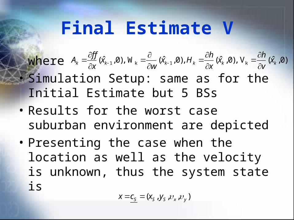
where

• Simulation Setup: same as for the Initial Estimate but 5 BSs

• Results for the worst case suburban environment are depicted

• Presenting the case when the location as well as the velocity is unknown, thus the system state is

1 k 1 kˆ ˆ ˆ ˆ( ,0), W ( ,0), ( ,0), V ( ,0)k k k k k k

f f h hA x x H x x

x w x v

( , , , )S S S x yx c x y

Final Estimate VI

• Assuming zero-mean Gaussian acceleration, the dynamics of the mobile are given by

where w1, w2 are white noise processes. In discrete time, the dynamics are given by

1 2 , , , s x s y x yx y w w

1 1 1 1 1

1 1 1 1 2

( ) ( ) ( )( ) ( ) ( ) ( )

( ) ( ) ( )( ) ( ) ( ) ( )

s k s k x k k k x k x k k k

s k s k y k k k y k y k k k

x t x t t t t t t t t w

y t y t t t t t t t t w

Final Estimate VII

in which f(.) is a linear and A is a 4x4 identity matrix

• For urban areas we take with Rayleigh distributed attenuation. In urban and suburban areas we take N between 2-6 with Nakagami distributed attenuation

6N

Final Estimate VIII

• Results for rural areas

Final Estimate IX

Conclusions

• Triangulation is an obstacle for location estimation

• Stand-alone methods are not consistent

• The algorithmic part of a method is important for TTFF

• A method should be robust against channel knowledge