Embed Size (px)
Citation preview

AN ENGINEERING STUDY OF A DIGITAL TACHOMETERAND ITS EFFECTS ON FEEDBACK CONTROL SYSTEMS
Georg W. Goeschel

Library
Naval Postgraduate S
Monterey, California 9
TGRADUATE SCHOOL
Monterey, California
5 rr
An Engineering Study of a Di
and its Effects on Feedbackgital Ta
ControlchometerSystems
by
Georg W Goescrlei
Th esis Advisor
:
Geor ge J. Thaler
Approved for public release; distribution unlimited.
T 164099


SECURITY CLASSIFICATION OF THIS PAGE (Whmn Data Entered}
REPORT DOCUMENTATION PAGE READ INSTRUCTIONSBEFORE complet::,g FORM
1. REPORT NUMBER 2. GOVT ACCESSION NO 3. RECIPIENT'S CAT ALOG NUMBER
*. TITLE (and Subtitle)
An Engineering Study of a Digital Tachometerand its Effects on Feedback Control Systems
S. TYPE OF REPORT a PERIOD COVEREOEngineer's Thesis; September
im6. PERFORMING ORG. REPORT NUMBER
7. AUTHOR)-
*;
Georg W. Goeschel
«. CONTRACT OR GRANT NUMBERft.)
9. PERFORMING ORGANIZATION NAME ANO ADDRESS
Naval Postgraduate SchoolMonterey, California 93940
10. PROGRAM ELEMENT. PROJECT. TASKAREA a WORK UNIT NUMBERS
II. CONTROLLING OFFICE NAME ANO ADDRESS
Naval Postgraduate SchoolMonterey, CAlifornia 93940
12. REPORT DATE
September 197413. NUMBER OF PAGES
96l«. MONITORING AGENCY NAME a ADORESSf// dllleranl trom Controlling Otllce)
Naval Postgraduate SchoolMonterey, California 93940
15. SECURITY CLASS, (ol Ihla report;
Unclassified15a. DECLASSIFICATION/ DOWNGRADING
SCHEDULE
16. DISTRIBUTION STATEMENT (ol thtt Raport)
Approved for public release; distribution unlimited
17. DISTRIBUTION STATEMENT (ol the abatracl entered In Block 30, II dlllarant from Report)
18. SUPPLEMENTARY NOTES
1». KEY WORDS (Contlnua on ravara* alda II nacaaaary and Identity by block number)
Digital Tachometer
20. ABSTRACT (Contlnua on ravarma mid* II nacaaaary and Identity by block number.)
High speed integrated circuitry can be used to realize a tachometer witha high sampling rate at slow speeds. This device would, under certainconditions, be useful in damping transients of fairly fast velocity- andposition control systems. After a treatment of the errors which are inherentin this device and other conventional tachometers, a comparative study ismade of the effects of digital tachometer on relatively simple feedbackcontrol systems. Methods to improve the response are studied.
DD l.jAN^S 1473 EDITION OF I NOV 68 IS OBSOLETE
(Pa^C 1) •/* 0102-014-6601I
SECURITY CLASSIFICATION OF THIS PAGE (IThan Data tntarad)


An Engineer ing Study of a Digital Tachometerand xts Effects on Feedback Control Systems
by
Georg V. ,GoeschelLieutenant Commander, Federal German Navy
M.S., Naval Postgraduate School, 1973
Submitted in partial fulfillment of therequirements for the degree of
ELECTRICAL ENGINEER
from theNAVAL POSTGRADUATE SCHOOL
September 1974

"75 v
5>f

Library
Naval Postgraduate SchoolMonterey, California 93940
ABSTRACT
High speed integrated circuitry can be used to realize a
tachometer with a high sampling rate at slow speeds. This
device would, under certain conditions, be useful in damping
transients of fairly fast velocity- and position control
systems. After a treatment of the errors which are inherent
in this device and other conventional tachometers, a
comparative study is made of the effects of digital
tachometer on relatively simple feedback control systems.
Methods to improve the response are studied.


TABLE OF CONTENTS
I. INTRODUCTION 12
A. OBJECTIVES OF THIS STUDY 13
B. METHODS USED IN THIS INVESTIGATION 14
II. THE DIGITAL TACHOMETER 16
A. PHYSICAL PROPERTIES 16
A. TRANSFER FUNCTION 18
1. Constant Period Sample and Hold Tachometer. 18
2. Digital Tachometer with Holding Device 20
C. COMPUTER SIMULATION OF TACHOMETER 21
III. ERROR ANALYSIS ....,.,.,. 23
A. SAMPLING PERIOD 23
B. ACCELERATION ERROR 25
1. Error for Constant Period Sampler 25
2. Error in Sampler counting Pulses 26
3. Error in Digital Tachometer 27
4. Truncation Error 28
5. Comparison of Acceleration Error andTruncation Error • 39
IV. USE OF THE TACHOMETER IN FEEDBACK SYSTEMS 32
A. GENERAL CONSIDERATIONS 32
3. VELOCITY CONTROL 33
1. First Order System 33


2. Second Order System 38
3. Third Order System 40
C. POSITION CONTROL 42
1. Second Order System 42
2. Third Order System •„ 44
V. CONCLUSION 46
TABLE 1 48
FIGURE 1 55
APPENDIX 87
COMPUTER PROGRAM 89
BIBLIOGRAPHY 95
INITIAL DISTRIBUTION LIST 96
FORM DD 1473 97

LIST OF TABLES
TABLE I. DAMPED SECOND ORDER SYSTEM 48
TAELE It. QUADRATIC SECOND ORDER SYSTEM 49
TABLE III. DAMPED THIRD ORDER SYSTEM 50
TABLE IV. UNDERDAMPED THIRD ORDER SYSTEM 51
TABLE V. THIRD ORDER POSITION CONTROL SYSTEM 53
TABLE VI. FREQUENCY RESPONSE OF THIRD ORDER SYSTEM 54


LIST OF FIGURES
Figure
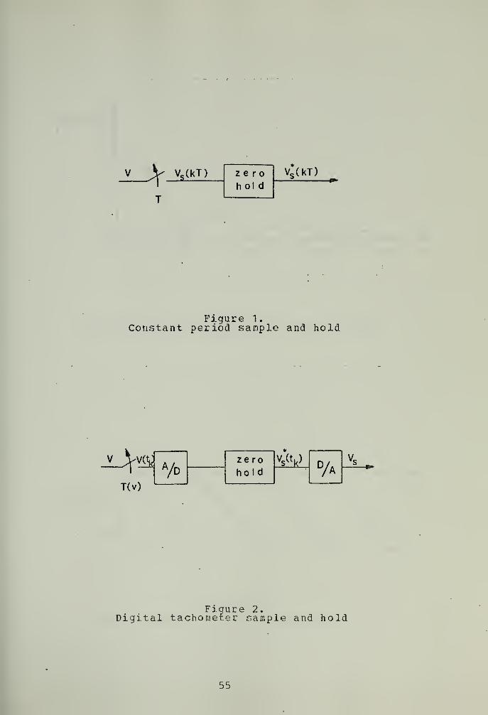
1. Constant period sample and hold 55
2. Digital tachometer sample and hold 55
3. Frequency response curve for sample and hold 56
4. Phase response curve for sample and hold 56
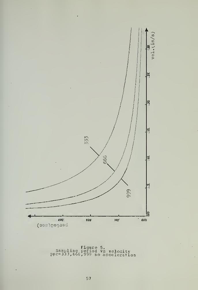
5. Sampling period vs velocity
ppr=333,666,999 no acceleration 57
6. Sampling period vs velocity
ppr=333 / 666 / 999 acceleration=100 in/s 58
7. Sampling period vs velocity
ppr=333,666,999 acceleration=1000 in/s 59
8. Sampling period vs time
velocity = 26 + 25sin (w*t) 6
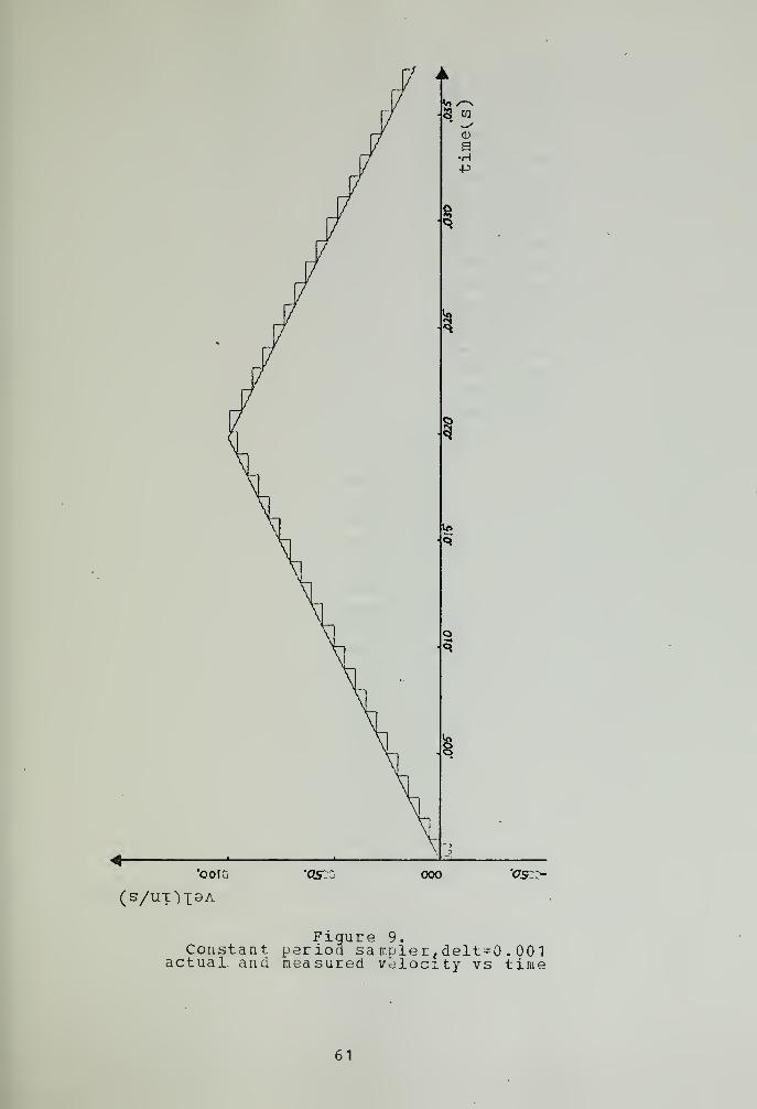
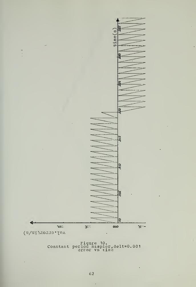
9. Constant period sampler, delt=0.001
actual and measured velocity vs time 61
10. Constant period sampler, delt = . 00
1
error vs time 62
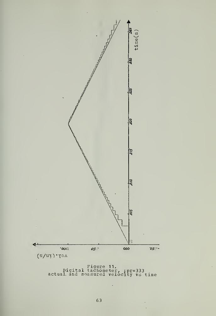
11. Digital tachometer, ppr=333
actual and measured velocity vs time 63
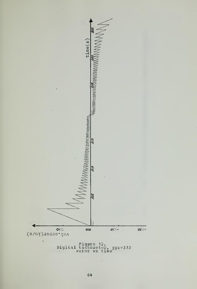
12. Digital tachometer, ppr=333
error vs time 64
13. Acceleration error vs velocity
ppr=333,666,999 acceleration^ 100 in/s 65
14. Acceleration error vs velocity
ppr=333 ,666,999 accelerat ion=1 000 in/s 66


15. Total error vs time, velocity=320 *t
acceleration error plus truncation error 67
16. Total error vs time, velocity=320*t
acceleration error only 68
17. Block diagram of first order velocity control 69
18. Block diagram for error analysis 69
19. 1st order system, ppr=167 input=25
analog=1, digital = 2, measured=3 70
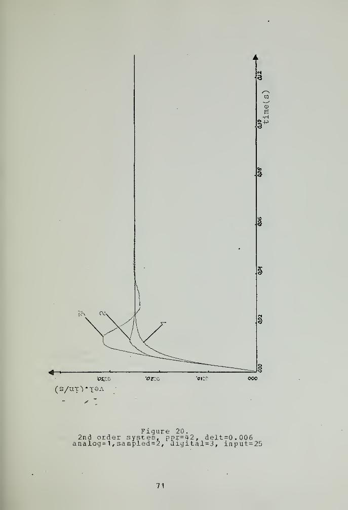
20. 2nd order system, ppr=42, delt=0.006
analog= 1 ,sampled=2, dicital=3, input=25 71
21. Quadratic 2nd order system, ppr=333, delt=0.001
analog=1, sarapled=2, digital=3, input=25 72
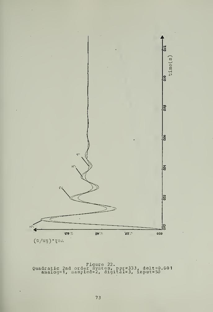
22. Quadratic 2nd order system, ppr=333, delt=0.001
analog=1, sampled = 2, digital = 3, input-50 73
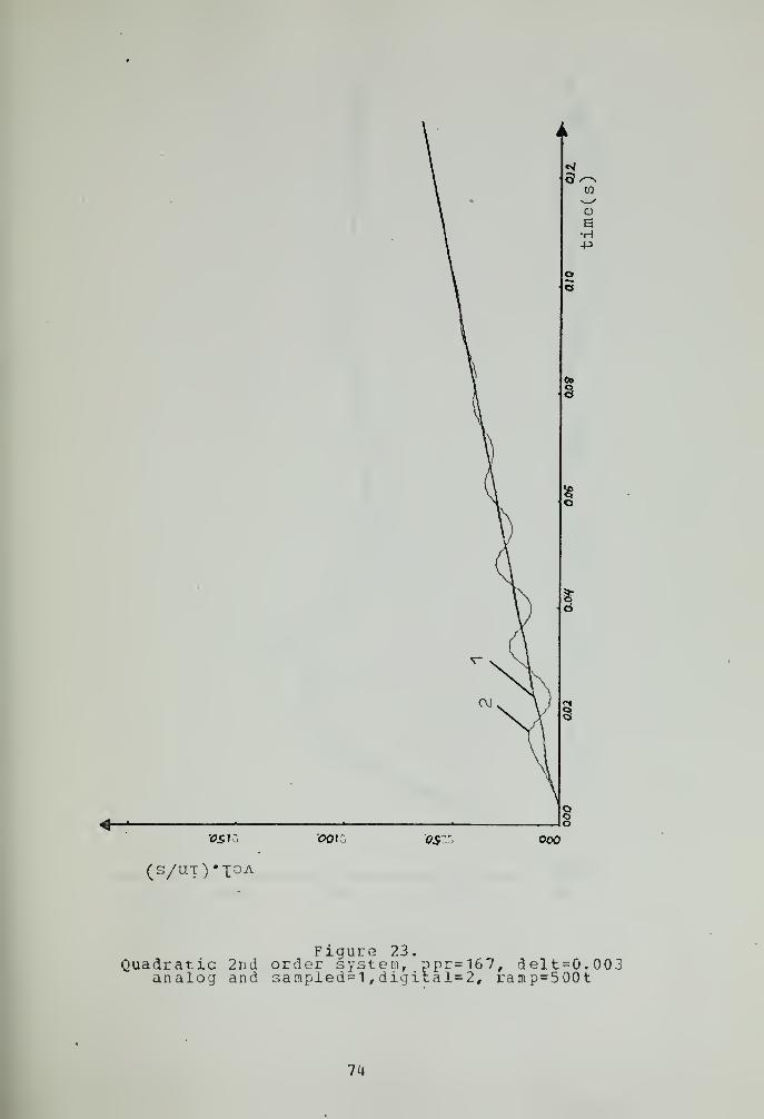
23. Quadratic 2nd order system, ppr=167, delt=0.003
analog and sampled= 1 ,digital=2, ramp=500t 74
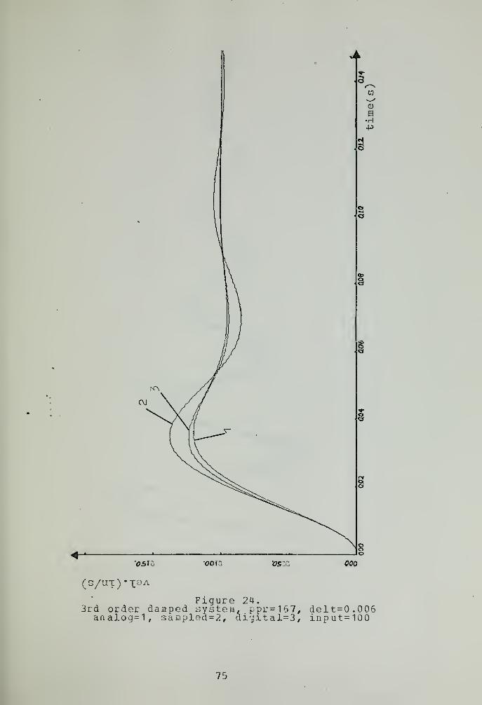
24. 3rd order damped system, ppr=167, delt=0.006
analog=1, sampled = 2, digital=3, input=100 75
25. 3rd order underdamped, ppr=167, delt=0.0005
analog = 1, sampled = 2, digital = 3, input=100 76
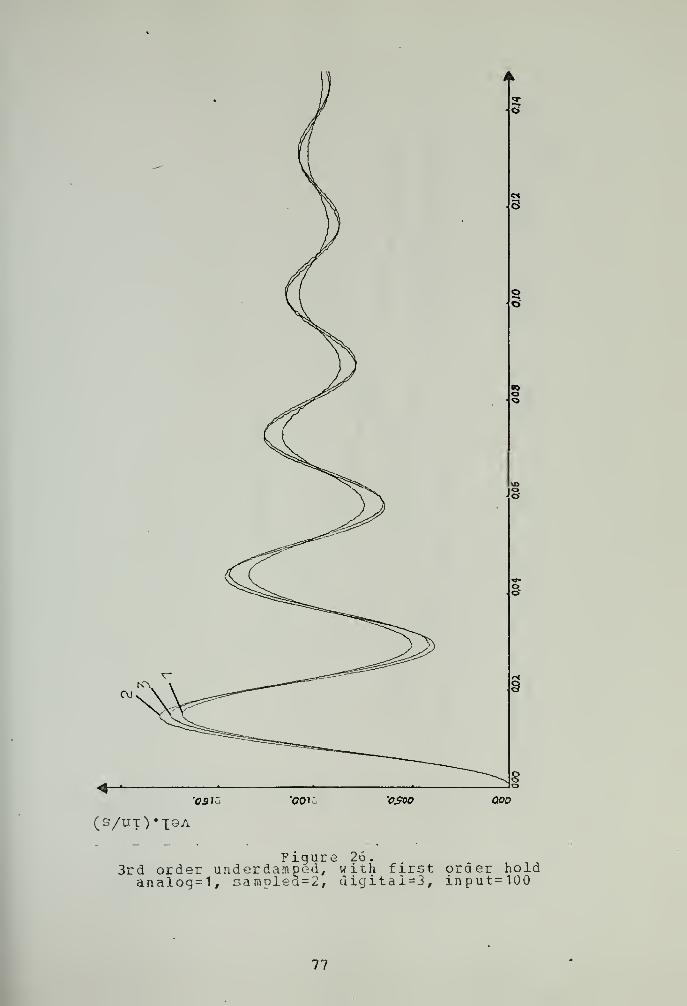
26. 3rd order underdamped, with first order hold
analog=1, sampled=2, digital=3, input=100 77
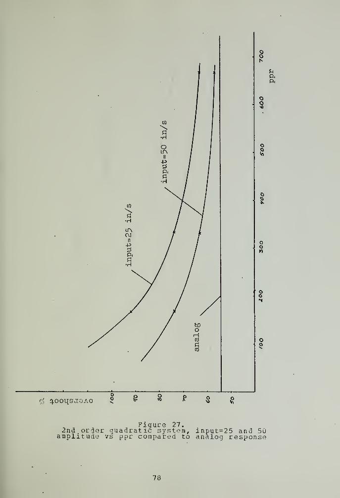
27. 2nd order guadratic system, input=25 and 50
amplitude vs ppr compared to analog response 78
28. 3rd order underdamped system, input=50 and 100
amplitude vs ppr compared to analog response 79
29. 2nd order position system, ppr=83, delt=0.01
analog=1, sampled = 2, digital = 3, input=0.5 80

30. 2nd order position system, velocity vs time
actual and measured velocity vs analog 81
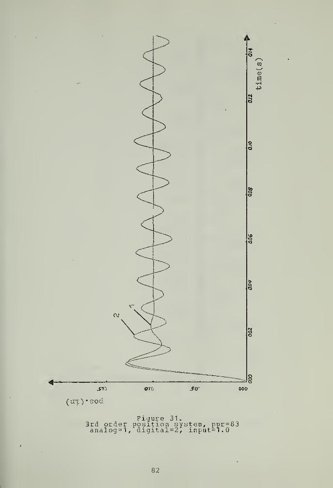
31. 3rd order position system, ppr=83
analog=1, digital=2, input = 1.0 82
32. 3rd order position system, velocity vs time
actual and measured velocity 83
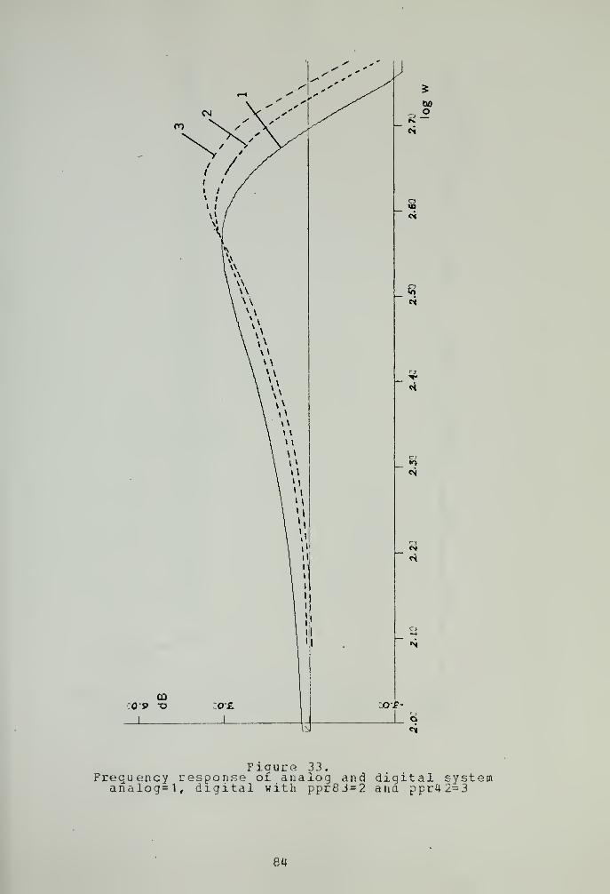
33. Freguency response of analog and digital system
analog=1, digital with ppr83 = 2 and ppr42 = 3 84
31. 3rd order position system, ppr=333, input=1.5
analog=1, digital = 2, zero order hold 85
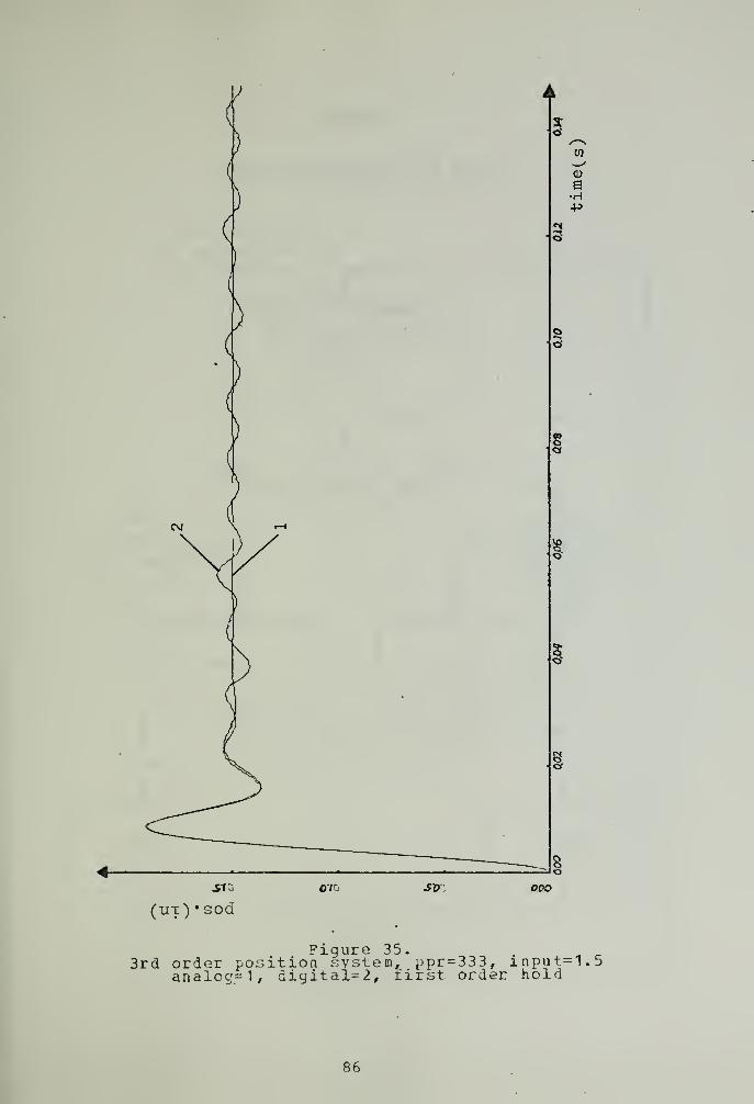
35. 3rd order position system, ppr=333, input=1.5
analog=1, digital = 2, first order hold 86
10

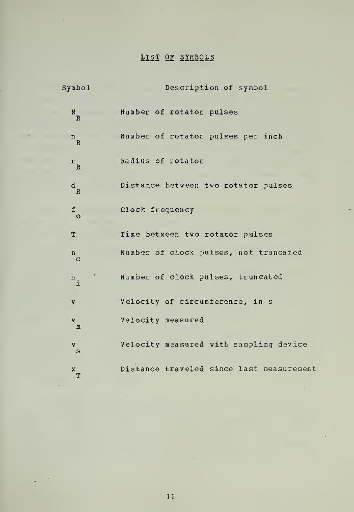
LIST OF SYMBOLS
Symbol Description of symbol
N Number of rotator pulsesR
n Number of rotator pulses per inchR
r Radius of rotatorR
d Distance between two rotator pulsesR
f Clock frequencyo
T Time between two rotator pulses
n Number of clock pulses, not truncatedc
n Number of clock pulses, truncatedi
v Velocity of circumference, in s
v Velocity measuredo
v Velocity measured with sampling devices
x Distance traveled since last measurementT
11


I • INTRO D UCT ION
Velocity feedback has been used for many years to
compensate control systems. It will make the transient
response of second and third order systems more desirable in
terms of peak overshoot and damping ratio. The steady state
performance for continuously varying inputs, however, will
in general be a little worse than without velocity feedback.
Fourth order systems will often require additional
compensation in the form of filters and will therefore not
be treated in this analysis.
Most tachometers used in such systems were either analog
measuring devices (Voltage generators) cr hybrid
digital-analog systems. In the digital-analog tachometer an
integration is used, based on counting the number of equally
spaced pulses on a transducer in a fixed, predetermined time
period, the so called sampling time. The number of counted
pulses is then directly proportional to speed. In order to
count a sufficient number of pulses, the sampling period has
to ne rather large ( in the order of 10-100 msec ), or the
number of pulses on the transducer disc has to be very
large, imposing difficult manufacturing procedures on the
manufacturer. Transducer discs with up to 20000 ppr are
available today. The slow sampling rates, however, do not
permit the use of these devices for transient analysis or
for measuring slow speeds.
Szabados,di Cenzo and Sinha (Ref.1) have introduced a
digital device, which is capable of measuring speeds
accurately enough from zero to high speeds and can easily be
made to measure negative velocities also. With simple
modifications it could also be used as an accelerometer.
12


This new device does not sample over equal time
intervals, however, but counts pulses of a fixed frequency
during equally spaced angular position intervals. The
number of frequency pulses is a direct measure of time.
Digital arithmetic devices then divide the known distance by
the time measured, and velocity results as output quantity.
This method has values of speed available after each
small distance interval, with only a small delay in the
arithmetic unit (20 microseconds ) . Therefore this device
is suitable for measurement of transients. To obtain
accurate measurements even at slow speeds, a constant rpra
"biasing motor" has to be used, which will complicate the
physical structure somewhat.
A. OBJECTIVES OF THIS STUDY
The proposed device seems to offer a rather cheap and
effective way to measure both transient and slow speeds. It
should therefore be possible to use it in control systems as
a compensating device, particularly in those applications,
where some digital computer is already available to do the
counting and the arithmetic.
Since this device samples at different time intervals,
depending on velocity, the well known z-transform method of
analysis and synthesis cannot be used here, and other
methods have to be found.
In order to get more insight into the particular
problems associated with the tachometer, an analysis of the
errors encountered was done first. These errors are
truncation error, due to integer counts, acceleration error,
occuring during acceleration between samples, and errors
related to the accuracy of the physical structure of the
13

device itself and the arithmetic unit.
The second objective was to study the effect of the
tachometer on feedback systems during dynamic phases. These
studies involved second order systems, and parameter changes
on the tachometer were used to outline their effects on the
system. All models were also studied with analog and
sampling feedback, so that excellent comparison was
possible. The primary objective was to find a relationship
between performance of the system and physical parameters of
the tachometer, how bandwidth affects the response and
whether the system would eventually become unstable. Later
it was attempted to limit or eliminate nonlinear effects by
using a first order hold feedback device.
B. METHODS DSED IN THIS INVESTIGATION
With the exception of a simple 4-bit arithmetic unit,
the total study was done in form of digital simulation on an
IBM 360 computer. The simulation of the tachometer proved to
be rather difficult, because an integration had to be done
in order to obtain the independent variable time, rather
than the dependent variable position, which was known in
advance in the form of the distance between tachometer
pulses. Although good results were obtained, a more
accurate and efficient integration would be necessary
whenever high speeds are involved.
For the design of appropriate systems, the
straightforward Root-locus and Bode plot procedures were
used. In order to study stability of a third order system,
it was deliberately designed to be unstable without
compensation and to have a fairly high natural frequency.
The tachometer was then used for compensation.
14


The following systems were simulated:
First order. Type 0, velocity control
Second order, Type 0, velocity control
Second order, quadratic, velocity control
Second order, Type I, position control
Third order , Type I, velocity control
Third order , Type I, velocity control
The following parameters were changed during simulation:
Number of pulses on tachometer disc ( Rotator )
Input amplitude
Poles of transfer function ( Bandwidth )
Delay time for sample and hold device
Clock frequency
The results were obtained both on graphs and as printed
output and are included, where appropriate, in tables and
figures
.
15


II. THE DIGITAL TACHOMETER
A. PHYSICAL PROPERTIES
The tachometer under consideration consists of a low
inertia, frictionless disc, called the rotator, which is
mounted tightly onto the shaft, the speed of which is to be
measured. Equally spaced openings around the circumference
of the rotator permit lignt to travel to a photodiode, which
will transmit pulses to a digital unit.
The digital unit consists mainly of a clock ( 2 MHz used
in this study) , a counter and an arithmetic unit. The
counter is initiated, stopped and reset by the incoming
pulses from the tacho disc. The count of clock pulses is
used in the arithmetic unit to derive the measured velocity.
The count is actually a measure of elapsed time between two
tacho pulses
n =£ (t -t )
c o k+ 1 k
and velocity is then
dR
v =ra (t -t )
k+1 k
Since the number of clock pulses depends on velocity, it
can be seen that this device will have small errors at slow
speed, although the actual resolution capability depends on
the number of pulses on the disc.
Most digital tachometers used so far did not use a clock
16


frequency as a basis to derive time, but counted the
tachometer pulses directly over one revolution or over a
specific sampling interval. If the sampling interval
remains constant, the velocity could be expressed in terms
of counted pulses
n 2TrrC R
V='N TR
and this equation could be used to calculate the number of
pulses per revolution required for a given resolution
capability at a given speed
n 2tttc R
N =-
R VT
From the equation it can be seen that these devices need
many pulses over one revolution for good resolution and
small error at slow speed. If the sampling is done at the
end of each revolution, the resolution is in the order of
one revolution per second, suitable for high speed devices,
but not useable as a measuring device for transient
analysis.
The activating pulses from the tacho disc have a varying
puisewidth, depending on the actual speed of the device. The
counter has therefore to utilize either the rising edge of
the pulse or a monostable vibrator must be used to get a
pulse with constant width. In the further treatment of the
tachometer the varying pulse width is therefore neglected.
The authors of reference 1 and 2 have used an additional
bias motor. The photodiodes were mounted on this motor
which was rotating with constant speed. In this way a
measurement of velocity was possible even at zero speed.
With bias speed high enough, negative speeds can also be
17


measured, however with decreasing accuracy. The velocity
equation has to be changed and becomes
dS
v = vm (t -t ) bias
k+1 k
Since the counter can only count integers, an error
results in deriving the velocity. This truncation error will
be treated in more detail in section III. 4 .
In order to use the result of the arithmetic unit, a
digital to analog (D/a ) converter has to be used, or the
result has to be further processed by a digital computer.
Errors involving those devices are neglected in this study.
In this study it was always assumed that the linear
velocity in inches per second was of interest, rather than
the angular velocity in revolutions per second. In most
cases the number of pulses per revolution was changed.
Since truncation error depends not only on velocity and ppr,
but also on the clock frequency, the latter had to be
changed occasionally in order to investigate effects of
truncation error on a system.
B. TRANSFER FUNCTION
1 . Constant Period Sample and Hold Tachometer
In order to point out the differences between the
two sampling devices, the derivation of the transfer
function for the sample and hold device is done in more
detail than actually necessary (Ref.3). For the block
diagrams see Fig. 1 and Fig. 2 .
18


The input to the holding device after sampling is
N
v (t)=Yv(kT) (t-t )
k =
The Laplace transform of this is
N
=1 -kTsv (s) = > v (kT) e
k=0
After the holding device, the output is a staircase like
function and can in time domain be written as
N
v (t) = ^v(kT) [u (t-kT) -u (t- (k+1) T)l
k=0
which laplace transformed becomesi
r— -kTs -Tsv (s) 2_v ( kT ) e ( 1_e )
s =
This can be further reduced, since the sampling time remains
constant. The final transfer function is therefore
v^- -kTs -Ts* > v(kT) e (1-e )V s) £o
v (s)
k=0
(kT) e•kTs
Or substituting jw for s, the freguency response can be
determinedT sin wT
~T~ -0.5jwTG (jw) = eHo wT
This is the well known function for the constant period
sampler.
19

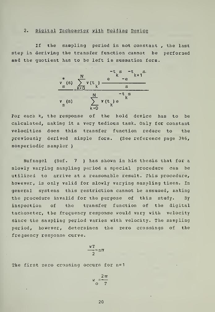
2« Digit al Tachometer with Holding Device
If the sampling period is not constant , the last
step in deriving the transfer function cannot be performed
and the guotient has to be left in summation form.
*V (s)s
N
_k--0
r(t )-
k
-t sk
e
-t s.k+1
-e
s
V (s)s
N
k--0
(t )ek
t sk
For eacc k, the response of the hold device has to be
calculated, making it a very tedious task. Only for constant
velocities does this transfer function reduce to the
previously derived simple form. (See reference page 346,
nonperiodic sampler)
Hufnagel (Ref. 7 ) has shown in his thesis that for a
slowly varying sampling period a special procedure can be
utilized to arrive at a reasonable result. This procedure,
however, is only valid for slowly varying sampling times. In
general systems this restriction cannot be assumed, making
the procedure invalid for the purpose of this study. 3y
inspection of the transfer function of the digital
tachometer, the frequency response would vary with velocity
since the sampling period varies with velocity. The sampling
period, however, determines the zero crossings of the
freguency response curve.
wT— = nn2
The first zero crossing occurs for n=1
_2tt
o T
20


It can be seen that for high velocities the sampling period
becomes short, effectively moving the freguency response
curve outward. For decreasing velocities the zero crossings
move inward, thus increasing or decreasing the bandwidth of
the tachometer, depending on speed. Associated with the
freguency response is of course the phase curve, which is
changing its steepness as the velocity varies. See also
Fig. 3 and Fig. 4 .
C. COMPUTER SIMULATION OF TACHOMETER
The computer simulation of the tachometer is based on
the only known quantity, the distance between two
tachopulses. The program calculates the linear distance
traveled by integrating the linear velocity, using discrete
steps of time. If the stepsize in time is kept too large,
the error in calculating the distance is not acceptable, a
large error in clock count would result. This in turn leads
to large truncation errors. In order to reduce calculation
time, a dynamic integration routine was used, which changes
the integration step size, depending on how close the
calculated distance traveled approaches the actual distance
between pulses. If the integration results in a larger
distance, the integration routine restores initial values,
reduces the step size and integrates again. This procedure
_ois done until the step size becomes less or egual 10
seconds. Then the velocity is finally derived and a large
step size restored. .
In the program, the variable CONCNT is the normalized
distance traveled, which truncated becomes actual tachopulse
count COUNT. The two variables RCOUUT and LCOUNT provide a
means of checking for the first arriving pulse after a start
or a reversal of velocity. Only if COUNT1 is egual to two,
21


does the program calculate the velocity, since the first
pulse cannot provide any correct velocity information.
In order to make the tachometer realistic, an initial
offset is added in the variable TACSH, taken to be 0.75 in
this study. This means, the distance to the first
tachopulse after the start of the simulation is 1-TACSH and
effectively shifts the velocity measurement in time.
The integration time is the period between two samples.
The number of clock pulses counted is then obtained and the
measured velocity derived by utilizing the previously
defined velocity equation. The program then returns,
simulates the system until a new tachopulse arrives and
calculates the new measured velocity.
A means of sensing direction is introduced by comparing
the last distance with the second last value. The sign of
this ccmparison determines the direction of rotation. In a
real tachometer, direction changes could be detected by
using a second marker string, displaced in phase with
respect to the first string. Depending on which pulse is
detected first, a change in direction can be sensed. The
program, the flow chart of the complete simulation and a
picture of actual versus measured velocity are shown in
appendix .
22


III. ERROR ANALYSIS
A. SAMPLING PERIOD
As previously mentioned, the sampling period for the
device under study is a nonlinear function of velocity. In
particular, for a constant velocity, the sampling period is
dR
t -t =—k+1 k v
This nonlinear dependence on velocity is plotted in Fig. 5 ,
where pulses per revolution (ppr) is a parameter. For low
velocities the difference in sampling period for small
velocity changes is very pronounced, whereas for high
velocities, the sampling period does not change
significantly with small velocity changes. However for the
same percentage of changes in velocity, the period will vary
the same percentage amount, regardless of the initial
velocity. This is shown in the example on the next page.
As will be discussed in a later section, the period will
also depend on acceleration during sampling intervals. This
can be seen in Fig. 6 and Fig. 7 , where the period is plotted
versus velocity, with acceleration as parameter. Fig. 8
snows clearly the drastic variations of sampling period as
the velocity changes sinusoidally v= 26+25sin (wt)
.
23


Example
Resolution = 333 ppr
Initial velocity = 10 and 50 in/s
Velocity variation^ t 1 in/sec
Velocity Period Percent
{in sec) (sec)
09 0.0020965 +11.1
10 0.001887 0.0
11 0.007715 - 9.09
49 0.000385 + 2. 04
50 0.000377 0.0
51 0.0003699 - 1.96
Velocity variation= -10 percent
Velocity Period Percent
(in sec) (sec)
09 0.0020965 +11.1
10 0.001887 0.0
11 0.007715 - 9.09
45 0.0004193 +11.1
50 0.000377 0.0
55 0.000343 - 9.09
24


B. ACCELERATION ERROR
In the previous section a constant velocity during a
sampling period had been assumed. Since the tachometer was
intended to measure transient behavior, this assumption
cannot be maintained. Accelerations between sampling
periods will occur and should be detected by the device. As
in all sampling devices, however, the velocity changes due
to accelerations cannot be measured instantaneously. Only
at the sampling time can a velocity measurement be made,
resulting effectively in a measurement of average velocity.
Very fast changes in velocity due to high accelerations
might not be detected at all. For the following error
analysis a constant acceleration during a sampling period is
therefore assumed and seems to be reasonable, at least for
high velocities, when sampling periods are short. Since an
investigation of truncation error will follow, truncation is
not included here for simplicity.
1 • Error for constant Per iod Sa mjaler
A device, which is essentially analog but measures
the actual velocity only at specific times, is a sampling
device with no error at the time of sampling. The error
during sampling intervals depends only on the behaviour of
the velocity during these periods (Fig. 9) . Any analog to
digital converter will have this error, if we neglect
guantization error due to digitizing the signal.
25


2. Error in Sampler counting Pulses
The velocity is now derived from counting marker
pulses on the tachometer disc during egual time intervals.
The number of pulses counted is a direct measure of distance
traveled. This number is dependent on the initial speed at
the start of the interval and the acceleration encountered
during that interval.
a 2x = v T+— TT o 2
The number of markers counted is
n =x Nc T R
The actual velocity is
v=v +aTo
whereas the measured velocity is
xT a
v =— =v+ T —m T 2
For this device there is an error during accelerated
regions, depending in magnitude on the amount of
acceleration and the sampling period.
ae=v-v =—
T
m 2
26

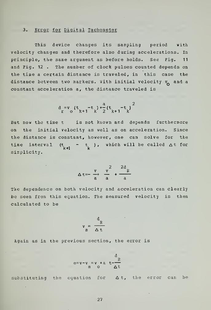
3« l££2I I2£ Digital Tachometer
This device changes its sampling period with
velocity changes and therefore also during accelerations. In
principle, the same argument as before holds. See Fig. 11
and Fig. 12 . The number of clock pulses counted depends on
the time a certain distance is traveled, in this case the
distance between two markers, with initial velocity v and a
constant acceleration a, the distance traveled is
a 2d =v (t -t ) +-(t -t )
r o k+1 k 2 k+1 k
But now the time t is not known and depends furthermore
on the initial velocity as well as on acceleration. Since
the distance is constant, however, one can solve for the
time interval
simplicity.
(t t ), which will be called At for
2 2dv v R
A t= + — +a a a
The dependence on both velocity and acceleration can clearly
be seen from this equation. The measured velocity is then
calculated to be
m At
Again as in the previous section, the error is
e=v-v =v +a tra o At
substituting the equation for A t, the error can be
27


expressed in terms of initial velocity at the start of the
sampling interval and the acceleration during the interval.
ad2 R
e= v +2adoR \(~2-v +\/v
o y o+ 2ad
R
A plot for acceleration error vs velocity with a given
acceleration and three different ppr is shown in Fig. 10 and
Fig. 11 . The error reduces significantly for high speeds.
Comparing this error with the error derived earlier, it can
be seen that the digital device will have less acceleration
error.
The acceleration error could also be viewed as a phase
shift, particularly in feedback systems. The measurement
follows a certain time later than changes may have taken
place, thus introducing a phase lag in feedback. This phase
lag, while known in a constant period sampler, cannot be
predicted for the digital tacho.
*• • Ji£liIl£stioiI l£E2£
In all digital devices, a certain amount of
information is always lost due to the guantizing nature of
the procedure. In the case of the tachometer, the counter
can only count integer numbers. Assuming a square wave clock
generator, the counter will be triggered either by the
leading or the falling edge. Fractions of cycles cannot be
counted. The sign of the truncation error will depend on
whether the count starts with the leading edge or the
falling edge of the pulse. In one case the count is higher,
in the ether case lower than the actual fraction would
indicate. The error will also depend on whether the clock
pulse generator starts with the arrival of the first tacho
28


pulse, or whether the generator is a continuously running
device. In the first case the count would only be truncated
at the end of the upcount, resulting in an error of at most
one count. In the second case the truncation could occur at
the beginning and the end of the upcount, leading to a loss
of two counts in the worst case.
The tachometer under study uses very small positional
increments for measuring speeds. At high speeds the sampling
times are very short. It can therefore be anticipated that a
truncation error might become rather pronounced at higher
velocities.
example
For a 2 MHz clock, a 333ppr tacho and a velocity of
50 inch per second, an error of one count (maximum)
results in a velocity measurement error of 0. 133 %
or 0.0663 13 in/s .
The truncation error is affected by all parameters given
in chapter II. It is inversely related to clock freguency
and radius of disc, and directly proportional to ppr and
velocity.
In the model used, the clock generator was assumed to
start with an incoming tachopulse with one count as maximum
error. The actual velocity is calculated with distance and
total count as
d fR o
v =nc
29


The measured velocity is
a fR O
n
Since the count starts with zero, the measured velocity will
therefore be slightly higher, assuming no acceleration
during the sampling period. As before, the error is
e=v-v =d f
(n.-n)1 c
m R o n ni c
For a count difference of one, a maximum error of
-1e =d fmax R o n (n +1)
i i
results. The percentage error is
e =(1 ) 100 %P n.
and the maximum percentage error
e = 100 %pmax n
i
The last equation indicates clearly the increasing
truncation error with increasing velocity (short count)
.
30


5. Compa rison of Acceleration Error and Truncation
Error
These two errors have different signs. While the
acceleration error is positive for positive acceleration and
negative for negative acceleration, the truncation error is
always negative. Moreover, the acceleration error decreases
with increasing velocity, whereas the truncation error
increases. Thus the total error resulting from these two
errors will vary with acceleration and velocity, the
truncation error becoming dominant as speeds increase. This
can be seen in Fig. 15 , where the error of slowly
increasing velocity ramp ( acceleration=320 in/s ) is shown.
A calculation of velocities in the vicinity of negative
errors clearly shows the effect of truncation.
Exat£lc
Velocity in in/s
actual : 60.424058 60.623579
measured without truncation : 60.374070 60.573776
measured with truncation : 60.378957 60.673374
Error=v-v in in/sm
without truncation : 0.049988 0.049816
with truncation : 0.045100 -0.049794
Number of cycles counted :625.05 622.988
In Fig. 16 , the same velocity was measured without
truncation, resulting in an even distribution of the error.
The decreasing width of the error curve indicates a decrease
in acceleration error since the sampling periods become
shorter. In preparing the last two curves, a bias motor with
50 in s was used.
31

IV. USE OF THE TACHOMETER IN FEEDBACK SYSTEMS
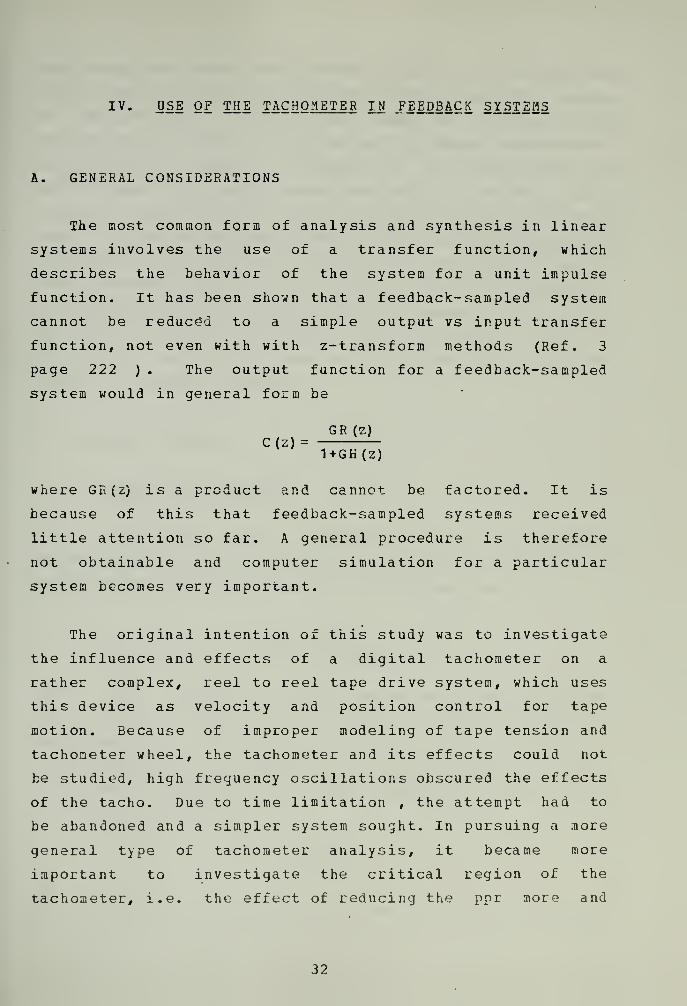
A. GENERAL CONSIDERATIONS
The most common form of analysis and synthesis in linear
systems involves the use of a transfer function, which
describes the behavior of the system for a unit impulse
function. It has been shown that a feedback-sampled system
cannot be reduced to a simple output vs input transfer
function, not even with with z-transform methods (Ref. 3
page 222 ) . The output function for a feedback-sampled
system would in general form be
GR (z)C(z) =
1+GH(Z)
where GE(z) is a product and cannot be factored. It is
because of this that feedback-sampled systems received
little attention so far. A general procedure is therefore
not obtainable and computer simulation for a particular
system becomes very important.
The original intention of this study was to investigate
the influence and effects of a digital tachometer on a
rather complex, reel to reel tape drive system, which uses
this device as velocity and position control for tape
motion. Because of improper modeling of tape tension and
tachometer wheel, the tachometer and its effects could not
be studied, high freguency oscillations obscured the effects
of the tacho. Due to time limitation , the attempt had to
be abandoned and a simpler system sought. In pursuing a more
general type of tachometer analysis, it became more
important to investigate the critical region of the
tachometer, i.e. the effect of reducing the ppr more and
32


more until the device would become useless. In the limiting
case, when only one pulse per revolution is used, the device
is the same as the one that measures the time of one
revolution in order to arrive at a speed measurement.
Increasing the number of pulses on the rotator makes the
device more and more compatible with a normal analog
feedback device and the usual methods of analysis could be
used. To get meaningful results for the simulation of
transients, the systems which were to be simulated had to
have reasonably high natural frequency and large bandwidth.
A frequency in the order of 50 Hz was thought to be typical
in electrical motors and servos. This assumption met with
the values which were used in the original paper from the
authors previously mentioned.
B. VELOCITY CONTROL
1 • ±.±E.§.±. 2I.Q~.IL System
From the block diagram of the originally
investigated tape drive, a linear version of one of the
drive motors provided a simple transfer function
23G(s) =
s(s + 0.25)
which was used in a first order velocity control system
(Fig. 17), calling for a 25 in/s nominal speed, or
eguivalent of 1.2 to 1.6 rev/s for a tape reel of 6 in
average diameter. This system is inherently stable without
overshoot. Modifying the block diagram as in Fig. 18 and
looking at the error
e = R-Cf
one can use the type zero error coefficients tc determine
33


the steady state error for an analog system and compare this
with results obtained from runs with a digital tacho.
Comparing the transient region first, however (Fig. 19),
it can fce seen that during the starting phase the velocities
in the system with digital feedback, are slightly higher,
since feedback lags behind actual velocity. The start is
even faster than in a system employing constant period
sampling with T=0.01 seconds. But since the digital tacho
decreases sampling time as velocity increases to 25 in/s,
the response of that system resembles more closely that of
the analog system as it approaches higher velocities. For a
ppr=167 and velocity=25 in/s the sampling period is 0.0015
against 0.01 for the sampler. A digital tacho with the same
sampling period at 25 in/s would only need 25 ppr. Such a
system would have a steep transient curve however. To
obtain fairly good resolution in a constant period sampler,
a ppr of about 2000 would be necessary, which would result
in a measurement of about 80 pulses per sample at the
nominal speed of 25 in/s. The truncation error is then
still larger than 1 %, and would further increase for slower
velocities.
Some comparative numbers
Time analog
0.01 5. 153
0.02 9.200
0.03 12.422
0.04 14.976
0.06 18.603
0.07 19.875
0. 10 22.313
0.20 24. 495
2.00 24.731
digital sampled
5.748 5.747
10.420 10.156
13.636 13.540
16.066 16.140
19.420 19.666
20.650 20.842
22.717 22.970
24.547 24.606
24.7 00 24.73 1
34


The shape of the transient depends also on the initial
offset of the tacho. If the first arriving pulse could
already be used for velocity measurement, then the response
would not be as steep as it is with a longer delay time at
the start. Until the first measurement, the system acts as
if there was no velocity feedback at all. Then the velocity
feedback sets in, however with smaller measured velocity
than the actual velocity. The difference between the
measured and true velocity is decreasing as the system
approaches nominal speed. This means the system acts as if
the feedback possesses a variable gain factor, starting with
zero and approaching one as velocity approaches nominal
velocity and accelerations go to zero.
The analog steady state error is calculated to be 0.2688
in/s for a step input of amplitude 25 and infinite for a
ramp input.
If a digital tachometer with the same gain constant
would be used, then the previously defined errors have to be
added. For a step input, only the truncation error adds to
the steady state error. For high velocities the truncation
error results in a velocity measurement higher than true
velocity and the error becomes even negative. This results
in an even larger steady state error than for an analog
system. To illustrate this effect, a large truncation error
was deliberately created by using a large number of pulses
(666) and a low clock frequency (0.2 MHz), the justification
for these numbers being shown below in the derivation.
The maximum truncation error was previously found to be
2rrr f (-1)R o
emax N n (n +1)
R i i
but we also know
35


2rrr fR o
= 25N (n +1)R i
and the error can be expressed as
-25
max ni
or with a given error
and then with f=0.2 MHz
-25n = = 93i e
max
2ttt fR o
= 534.7Re n (n +1)
max i i
The steady state error which now resulted was 0.494 in/s.
Count variations due to truncation might even result in
a limit cycle at the output. Final velocity as well as the
occurance of a limit cycle depends on the dynamics of the
system. In some of the velocity control systems and in all
position control systems a limit cycle was actually observed
and will be pointed out in the discussion of those systems.
The added error from the digital tachometer will become
more and more dominant for a ramp input, since in this case
the velocity increases and the truncation error will become
rather large. This can be shown easily using time domain
analysis.
36


For a ramp input of 1000*t, the function for velocity is
-23.25tC (t)=42.548(e +23925t-1) in/s
the error for an analog system after one second is
e=1000-946. 699=53. 3 in/s
For a digital tachometer with 666 ppr and 2 MHz clock
freguency, a maximum error of
e =1000-v =3.25 in/smax m
would result. It is assumed that acceleration error becomes
negligible at these speeds. After two seconds the maximum
error due to truncation would even be -129.6 in/s instead of
+106.6 in/s due to steady state error. This would result in
a lower velocity at the output and the error would increase
faster than in an analog system.
The last calculations and results show clearly three
facts. First, the feedback gain is variable during
transients, due to acceleration error, which depends on the
input amplitude. Second, truncation error may become rather
large and dominant, and third, it is better to use a small
number of tachopulses for high speeds, because this reduces
the truncation error. A steady state error analysis in the
conventional form as used in analog , unity feedback systems
cannot be used whenever high velocities are involved.
37

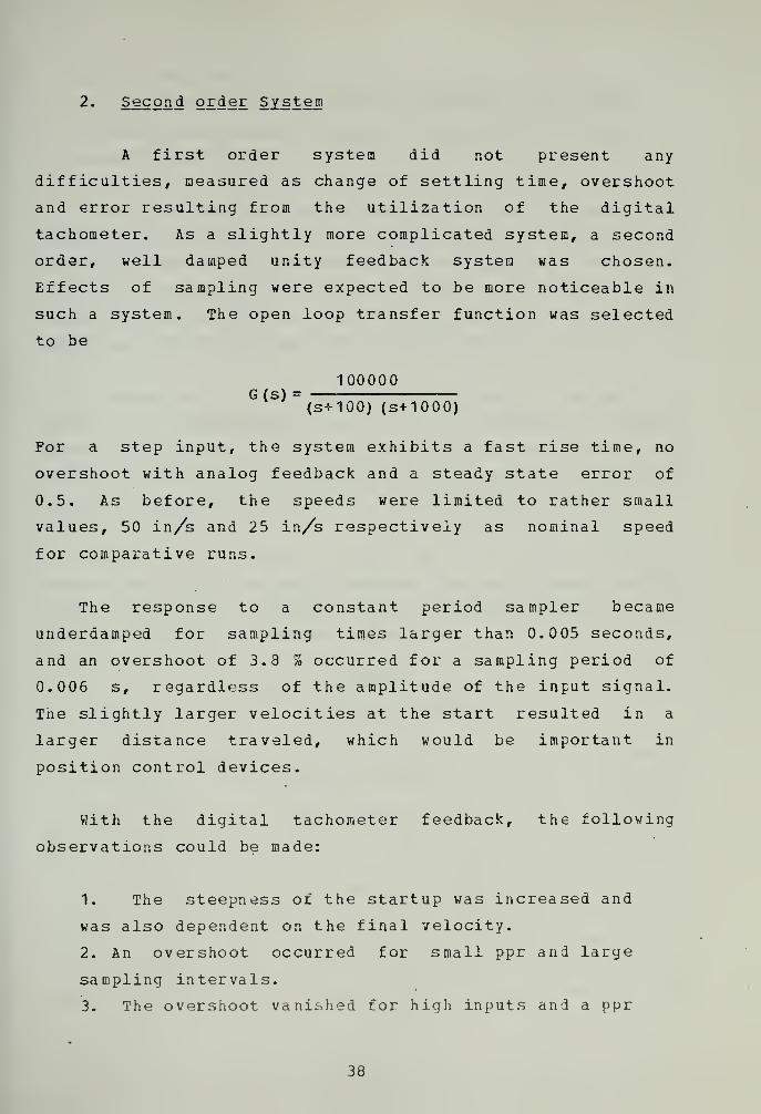
2« Second order System
A first order system did not present any
difficulties, measured as change of settling time, overshoot
and error resulting from the utilization of the digital
tachometer. As a slightly more complicated system, a second
order, well damped unity feedback system was chosen.
Effects of sampling were expected to be more noticeable in
such a system. The open loop transfer function was selected
to be
G(s) =100000
(S+100J (s+1000)
For a step input, the system exhibits a fast rise time, no
overshoot with analog feedback and a steady state error of
0.5. As before, the speeds were limited to rather small
values, 50 in/s and 25 in/s respectively as nominal speed
for comparative runs.
The response to a constant period sampler became
underdamped for sampling times larger than 0.005 seconds,
and an overshoot of 3.8 % occurred for a sampling period of
0.006 s, regardless of the amplitude of the input signal.
Tne slightly larger velocities at the start resulted in a
larger distance traveled, which would be important in
position control devices.
With the digital tachometer feedback, the following
observations could be made:
1. The steepness of the startup was increased and
was also dependent on the final velocity.
2. An overshoot occurred for small ppr and large
sampling intervals.
3. The overshoot vanished for high inputs and a ppr
38

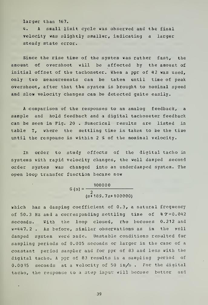
larger than 167.
4. A small limit cycle was observed and the final
velocity was slightly smaller, indicating a larger
steady state error.
Since the rise time of the system was rather fast, the
amount of overshoot will be affected by the amount of
initial offset of the tachometer. When a ppr of 42 was used,
only two measurements can be taken until time of peak
overshoot, after that the system is brought to nominal speed
and slow velocity changes can be detected guite easily.
A comparison of the responses to an analog feedback, a
sample and hold feedback and a digital tachometer feedback
can be seen in Fig. 20 . Numerical results are listed in
table I, where the settling time is taken to be the time
until the response is within 2 % of the nominal velocity.
In order to study effects of the digital tacho in
systems with rapid velocity changes, the well damped second
order system was changed into an underdamped system. The
open loop transfer function became now
100000G(s) =
2(s+189.7s+100000)
which has a damping coefficient of 0.3, a natural freguency
of 50.3 Hz and a corresponding settling time of 4T = 0.042
seconds. With the loop closed, rho becomes 0.212 and
w=447.2 . As before, similar observations as in the well
damped system were made. Unstable conditions resulted for
sampling periods of 0.005 seconds or larger in the case of a
constant period sampler and for ppr of 83 and less with the
digital tacho. A ppr of 83 results in a sampling period of
0.0015 seconds at a velocity of 50 in/s . For the digital
tacho, the response to a step input will become better and
39


better as the pulses on the disc increase, the specific
response depends on the amplitude of the input however. A
small limit cycle was observed, which was to be expected,
since the system is underdamped and truncation error does
not permit the system to stabilize itself. Initial offset at
the start does not affect the response in any noticeable
way.
For a ramp input, the response of the digital tacho
feedback system is not nearly as good as for the analog
system or even as for the constant period sampler. At the
start, the velocity is slow and only very few measurements
will be taken. This resulted in a rather oscillatory start
until at higher speed the sampling rate increases to
acceptable values and the system behaved like the other two
systems. A plot of tne response to a ramp input is provided
in Fig. 23 , where this effect can clearly be seen. In
Table II, the results of a second order guadratic system are
listed for step inputs.
3* ^hird order system
Adding a pole at zero resulted in a third order
system and the gain was first chosen to keep the system
slightly underdamped.
G(S)10000000
s (s+100) (s+1000)
The nominal speed was 100 in/s and 50 in/s , which permits
rather high sampling rates at full speed and a reasonably
good result could be expected. From Fig. 24 it can be seen
that for a ppr of 167 and larger, the response is close to
the analog response. Because the system was stable under
closed loop conditions, it was hard to reach large
overshoots, even with ppr as low as 42. For a constant
period sampling device, a sampling rate of 1000 samples per
40


second would be necessary to achieve the same response, and
for good accuracy a ppr of about 6000 would be needed.
With the gain increased to 5*10 , a very poorly damped
system resulted, requiring a faster sampling rate for good
response. With 42 or 83 ppr on the tacho disc, the response
was virtually unstable, although the oscillations did not
increase amplitude after they reached a final value. As can
be deduced from Fig. 25 , a reasonable response is only
achievable with a large number of pulses. A limit cycle
occurs and is larger than in other cases because the system
dynamics are much more unstable.
In order to reduce truncation error, a change in clock
freguency was also investigated. A freguency of 20 MHz did
affect the response only minimally. The peak overshoot
which resulted was 72.8 % compared with 72.5 % with larger
truncation error. But since the error is negative it reduces
the overshoot. A further reduction in clock freguency to 0.2
MHz produces even larger truncation error. With a ppr of
666 , the resulting count at full speed is only about
20, which means a 5 % error when one count is lost. In the
system, this large error caused only 69.15 % overshoot, a
considerable reduction compared to the previous runs. Again,
a listing is provided in Table IV .
As pointed out in an earlier chapter, a possible way to
improve the digital tachometer is to replace the holding
device by a first order hold, which would integrate between
samples according to the rate of change of measured quantity
between the two latest samples. The equation of measured
velocity is than
(v -v )
k-1 k-2v =v+ *(t-t )
m k (t -t ) k-1k-1 k-2
41

Table IV includes the results of a run with a first order
hold in the feedback path, and an improvement can be
observed when comparing the Fig. 26 with Fig. 25 . The
improvement did not change the settling time, however. This
can be attributed to the occurrence of the limit cycle. The
response to a ramp is very poor at the beginning as in the
second order system.
The amount of overshoot depends not only on the
characteristics of the plant, but also on the parameters of
the feedback device. A plot of peak amplitude vs ppr for
two particular systems is shown in Fig. 27 and Fig. 28 . A
definite relationship to the input amplitude can clearly be
seen. Although for each input a new curve would have to be
drawn, intermediate values are easy to interpolate from the
curves available. This was actually done and the result was
as predicted. Finally it can be said that all velocity
control systems had a slightly faster start when using the
digital tacho, and the peak time was slightly less than with
either analog or constant period sampling feedback.
C. POSITION CONTROL
1 . Second order System
In a position control system, the tachometer is used
for compensation in case the response would be too
underdamped or even unstable with unity feedback only. The
third order system chosen later was therefore designed to be
unstable without the tachometer compensation.
The same arguments concerning rise and settling time as
with velocity control systems apply and the first system was
a second order, type I, unity feedback system with transfer
function
42


G(S) =111100
s (s+100)
which then used tachometer feedback with a gain of 0.0009,
The total transfer function became then
G(s) =111100
s +200s+111100
with a natural frequency of 53 Hz and a rho of 0.3 r which
results in a peak overshoot of 37.2 % in an analog system.
In Fig. 29 , the response of various types cf velocity
feedback to a step input is shown. The velocity will
eventually go to zero, and a plot of velocity vs time for
this system is included in Fig. 30 , where the smooth curve
is the actual velocity and the staircase curve the measured
velocity. The following observations are possible on this
simple system:
1. The peak amplitude with digital feedback is
slightly smaller than in the analog system for all
values of ppr chosen, while for the constant period
sampler the amplitude increases.
2. The bandwidth increases as can be seen by the
increased natural frequency. This effect was
predicted in chapter II. The freguency changed to
59.5 Hz with ppr of 83 and to 53.7 with a ppr of
666, approaching the response of the purely analog
system without tachometer feedback as the position
reaches the final value.
3. The response exhibits long ringing (limit cycle)
,
since at steady state no velocity feedback exists,
as can be seen in Fig. 30 .
In analyzing the phenomena observed when digital
feedback is used, the tacho gain factor has to be considered
variable. It will vary from zero at the start to the chosen
t\3


value for analog velocity feedback and even to a value
larger than the chosen one when the acceleration is
negative, because of the phase lag in measurement. The
larger gain factor could account for the reduced peak
amplitude. The peak occurred when the velocity changes
direction, i. e. after the system went through a period of
negative acceleration. Since the acceleration error depends
on initial velocity at the instant of sampling and on the
ppr, its effect should be reduced whenever the systems
dynamics involve high velocities. In a positioning system,
velocities are a function of input amplitude. Therefore the
percentage overshoot should also be a function of input
amplitude for a digital feedback system. Only with high
velocities will the truncation error affect the response.
2« £hird 2£<|sr Position Control System
In order to study the observed effects more
thoroughly, an originally unstable third order system was
compensated with a tachometer which used a gain of 0.00215.
The transfer function became then
G(s)1.5 10
8oo 8s +1100s +U22500S+1.5 10
with open loop poles at zero, 100 and 1000, and a natural
freguency of 58 Hz. The previously mentioned dependency on
input amplitude was now confirmed by using several input
sizes. Table V contains a listing of peak amplitude and
limit cycle amplitude for various step inputs. It can be
seen that the response depends on input amplitude and, as
was the case in the second order system, the peak became
actually smaller than the analog systems overshoot for
inputs larger than one and virtually all ppr values
selected. For small inputs, the response must be considered
unstable, since violent oscillations occur with amplitudes
44


comparable to the input step size. It was interesting to
note almost the same amount of overshoot at 4 times the
input amplitude with 1/4 th oi"-t,v:« ppr, as seen with ppr of
83 and input 2.0 vs a ppr of 333 and input 0.5 inches. Since
the system was unstable without tachometer, a limit cycle
resulted, because at steady state the feedback gain reduces
to zero for a step input. This limit cycle is independent of
input amplitude and depends on ppr and the systems dynamics.
Its amplitude was about 0.04 in with a ppr of 333 and 0.15
in with a ppr of 83, not exactly a 4:1 relationship. The
frequency of the limit cycle is again slightly higher than
the natural frequency. Fig. 31 and Fig 32 show the position
and velocity response to an input of 1.0 inch.
In order to find the frequency response curve, a series
of runs was made with several frequencies and different
tachometer parameters. Numbers are presented in Table VI,
while a plot of two frequency curves is shown in Fig. 33
It can be seen that the frequency response curve is not only
shifted to the right (increased bandwidth ), but also
changes in gain. While the gain is lower for frequencies
less than the natural frequency, it increases for higher
frequencies until it falls off. It has to be indicated again
that during a particular transition the frequency response
is dynamically changing, depending on the form of the input,
i. e. differently for a step input, a ramp or other input
functions.
For a ramp input, this system behaves like a stable
velocity control system with a step input, and a treatment
of ramp input response is therefore omitted. An attempt to
improve the response by using a first order hold feedback
was also made. But while the transient resembles now more
closely the response of an analog system, the steady state
response is worse in that the the limit cycle becomes larger
in an irregular way, as can be seen in Fig. 34 and Fig. 35 .
45


v - CONCLUSION
The proposed tachometer has characteristics which are
superior to all velocity sampling devices previously used.
If carefully designed, it will be helpful in compensating
velocity and position systems. It is important, however, to
choose the parameters of the tacho according to the nominal
operating region of the system, since the output of the
tacho depends on input amplitude. As the authors of Ref. 1
point out, a bias motor will greatly improve the response
because it allows measurement even at zero velocity. Since
the sampling rate is very high, an analog system analysis
should in most cases be justified.
Under certain conditions and with careful design, it may
be possible to use the truncation error as an aid to
damping. This had been demonstrated in chapter IV. C 2 .
It is furthermore easy to use a second counter to count
the number of rachopulses since the start, which then
provides position information as well.
Whenever high velocities have to be measured, a very
high clock freguency would have to be used in order to
reduce the truncation error. If, however, a reasonable
number of tachopulses could be utilized, then one can divide
the full operating region into two portions, using the
proposed tachometer at startup and slow velocities, while
switching to a regular sampls and hold tachometer at high
speed. The sample and hold device would then still get
enough pulses to provide good resolution.
Another possible application of the tachometer uses
previous peasurements to obtain an estimate of acceleration.
U6


Since the digital tacho provides data at a fairly high rate,
the acceleration measurement should be rather accurate and
the obtainable resolution superior to the sampling and
counting routines used so far.
From the previous conclusions it can be seen that the
use of the digital tachometer leaves many areas to be
studied. The author believes that further study of the
mathematical analysis is necessary. Another suggested field
of investigation is the actual design of the arithmetic unit
with the newest integrated circuits available. An
interesting aspect of this would be the possible use of a
microprocessor as a control unit and, may be, even as the
arithmetic unit itself. It is felt that with the reduction
of prices for single units and the incorporation of memory
into the processor, a fairly cheap but accurate digital
tachometer could be built.
47


TABLE I
analog
DAMPED SECOND ORDER SYSTEM
time of peak % overshoot settling time
0.0175
sampled
delt=0.001
delt=0.003
delt=0.005 0.0131 3.96
0.0175
0.013
0.015
digital
ppr= 42
ppr= 83
ppr=167
ppr= 42
ppr= 83
ppr=167
input=25 in/s
0.0141 25.84
0.011
0.014
17.6
0.452
input=50 in/s
0.011 10.65
0.012 1.8
0.0036
0.0195
0.0098
0.0191
0.0085
0.015
48


TAriLE II
analog
QUADRATIC SECOND ORDER SYSTEM
time of peak % overshoot settling time
0.00718 54.2 0.042
sampled
delt=0.005 0.0071 101.2 long
delt=0.003 0.0071 83.0 0. 152
delt=0.001 0.0071 62.0 0.058
digital
ppr=167
ppr=333
ppr=666
input=25 in/s
0.00708 91.7
0.00704
0.00705
73.9
63.2
0. 166
0.072
0.052
ppr=167
ppr=333
ppr=666
input=50 in/s
0.00701 73.8
0.00709
0.00707
63.0
57.0
0.060
0.051
0.044
49


TABLE III
analog
DAMPED THIRD ORDER SYSTEM
time of peak % overshoot settling time
0.0361 20.38 0.085
sampled
delt=0.006
delt=0.003
0.0351
0.0351
28.80
38.35
0. 110
0. 143
digital
ppr= 42
ppr= 83
ppr=167
ppr=333
ppr=666
input=100 in/s
0.0330 36.03
0.0340
0.0351
0.0355
0.0360
28.9
24.4
.22.4
21.36
0. 177
0.086
0.086
0.085
0.085
50

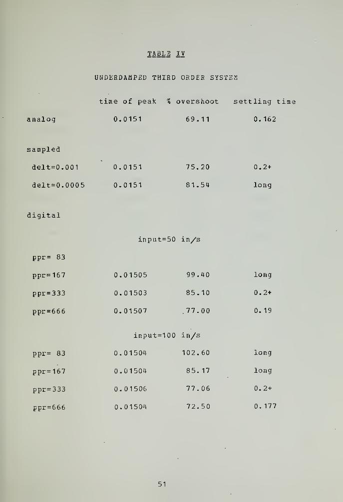
TABLE IV
analog
UHDERDAMPED THIRD ORDER SYSTEM
time of peak % overshoot settling time
0.0151 69.11 0.162
sampled
delt=0.001
delt=0.0005
0.0151
0.0151
75.20
1 .54
0.2 +
long
digital
input=50 in/s
ppr= 83
ppr=167
ppr=333
ppr=666
0.01505
0.01503
0.01507
99.40
85.10
77.00
long
0.2+
0. 19
ppr= 83
ppr=167
ppr=333
ppr=666
input=100 in/s
0.01504 102.60
0.01504
0.01506
0.01504
85. 17
77.06
72.50
long
long
0.2 +
0. 177
51

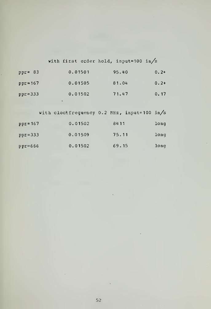
with first order hold, input=100 in/s
ppr = 83 0.01501 95.40 0.2+
ppr=167 0.01505 81.04 0.2+
ppr=333 0.01502 71.47 0.17
with clockf requency 0.2 MHz, input=100 in/s
ppr=167 0.01502 8411 long
ppr=333 0.01509 75.11 long
ppr=666 0.01502 69.15 long
52


TABLE V
THIRD ORDER POSITION CONTROL SYSTEM
input % overshoot % limit cycle
analog 27.34
digital ppr=333 ppr=83 ppr=333 ppr=83
0.25 28.98 46.34 13.77 65.956
0.50 27.76 34.10 6.40 29.800
1.0 27.39 29.51 3.84 15.57
1.5 27.16 28.39 2.8 9.325
2.0 26.85 27.90 1.8 8.18
53


TABLE VI
FREQUENCY RESPONSE OF THIRD ORDER SYSTEM
frequency amplitude in dB
analog ppr=333 ppr= 83 ppr= 42
20 0.445 0.366 0.121 -0.087
30 0.867 0.765
40 1.756 1.613
50 2.652 2.542
60 3.020 3.033
70 2.130 2.245
80 -0.028
90 -2.722 -2.270
100 -5.449 -5.036
110 -7.851 -7.535
0.473 0.374
1.356 0.668
2.280 2.007
3. 107 3.106
2.8G6 3.522
1.214 2.212
1.7170 -0.354
3.835 -2.854
6.410 -5.680
54

v \ W) zerohoi d
V-(kT)
Figure 1.Constant period sample and hold
SJf^T(v)
Vbzerohold
^_ D'A
Figure 2.Digital tachometer sample and hold
55


GHo
(jw)
Figure 3.Frequency response curve for sample and hold
Figure 4.Phase response curve for sample and hold
56

81
CO\c•H
r-1
CD
>
in
COO' roo 700'
o
O
000
Figure 5.Sampling period vs velocity
ppr=333,666,999 no acceleration
57


5W.'GGS^pOTaGCi
0T0- .SCO- OP*
Figure 6.Sampling period vs velocity
ppr=333, 666,999 acceleration=100 in/s
58


500'
(o9S)poxj:ad
-wo" z«r ooo
Figure 7.Sampling period vs velocity
ppr=333,666, 999 acceleration=1000 in/s
59


CD
E•H-P
Of
Of
eoo' 9oo" H>o' 700' 000
Figure 8.Sampling period vs timevelocity=26+25sin (w*t)
60

rV' ^
1 / <§ CO
CD
S•H-P
S^
rf
1
Qo
id — .. , . , 3
OOK
(S/UT")X8A
'Ost: ooo 'Os:>
Figure 9.Constant period sa rnpler , delt-0 . 00 1
actual, and measured velocity vs time
61

t
w'
a•H-P
k____"
^T^~~"r
^-——^"~~~_
___- "
__—^_—~
""""
l^-r^~^~__-— """
___-—-—"""
__^—~~
SI—-——"""""""
^__---—~^
_^—-—"""'"'
___^—-"""
__-—-—
~
o ^____~*
~~—~—-^"~~ -—___^ ^_ vn
^~~~~~ __~~~~ -—___"——-—__——-^^ -__ -1^^ __
~~" —-__~"~~ —
^_^~~~---—
___~~"
—__ uo^~-~^_
"""—__
~"-~—-^__-___
«— ."~~~^--— §
•oi:
( S/UT ") JOJJ8 * "[8
A
O00 "JBM-
Figure 10.Constant period sampler , delt=0. 00
1
error vs time
62

J / i k
* 1/?3
0>
s•H-P
J7
1In
3
3
In
o•**
Y^_i i i .
•OOTG
(s/ux") 'xoa
OS 000 osr-
Figure 11.Digital tachometer, ppr=333
actual, and measured velocity vs time
6 3

B•H-P
Vs
c*5
01:
(s/UT)joo:a:9 , xoAooo <nr ozs-
Figure 12.Digital tachoaeter, ppr=333
error vs time
64


S CO
N.Pi
•H
CD
>
o
o
ONK\ KD C^res kD C>
s
0*1: J'OO ooo
Figure 13.Acceleration error vs velocity
ppr=333, 666, 999 acceleration^ n;it y. /00 m/s
65


as. .
(s/ui'ijoaja
Figure 14.Acceleration error vs velocity .
ppr=333,666, 999 accelerat ion= 1000 in/s
66


(S/UI)J0JJ9
Figure 15.Total error vs tine, velocity=320*t
acceleration error plus truncation error
67


CQ
s•H-P
1st
I
o
—
*
In
(S/UX)JOJJ3
ro;, ro- OQO
Figure 16.Total error vs time , velocity=320 *t
acceleration error only
68


V(s)
I
1
1
di'g ital UI TachoI
Figure 17.Block diagram of first order velocity control
X(s)fr>
Figure 13.Block diagram for error analysis
69


Figure 19.1st order system- ppr=167 input=25analog=1, digital=2, measured=3
70

w
S3
•Ho is,3^
Figure 20.2nd order system, ppr=42, delt=0.006
analog=1 , sampled=2, diyital=3, input=25
71


(j/tttVISA
Figure 21.Quadratic 2nd ordsr system, ppr=333, delt=0.001
analog=1, sampled=2, digital=3, input=25
72

0* -r, 0*
(g/ut) *xsa
Figure 22.Quadratic 2nd order system, ppr=333, delt=0.001
analog=1, sampled=2, digital=3, mput = 50
73

3
(D
E•H-P
o-4o
09
!So
Q
OJ.
Qoo
(s/ut) *xoa
oor: <?.S~ ooo
Quadraticanalog
Figure 23.2nd order system, ppr=167, delt=0.003and sampled=1 , digital=2, ramp=500t
7a

est csx 000
(s/ui) 'x^a
Figure 24.3rd order damped system, ppr=167, delt=0.006analog=1, :5ampled = 2, digital=3, input=100
75


w
CD
e•H-P
(s/ut) *xsa'cot; <75~- 000
rigure 25.3rd order underdamped, ppr=167, delt=0.0005analog=1, sampled=2, digital=3 / input=100
76

5
8
'as re 'ooi: 'osoo QOO
(s/ut) 'xqa
Figure 26.3rd order under dam ped, with first order holdanalog=1, samoled=2, uigitai=3, input=100
77

uftft
Figure 27.2nd order quadratic system,
amplitude vs ppr compared toinput=25 and 50analog response
78


oo
ftft
oo
oO
oo
oo
o
'' q.OOl{SJ3AO
Figure 28.3rd order underdamped system, input=50 and 100amplitude vs ppr compared to analog response
79


w
E•H-P
so, 03 Mr 000
(ut ") -sod
Figure 29.2nd order position system, ppr=83, delt=0.01dnalog=1, satnpled = 2, digital=3, input=0.5
80


-00l •0S-^
(S/UT) *X3A
Figure 30.2nd order position system, velocity vs time
actual and measured velocity vs analog
81

6
CQ
e•H•P
inti
(ui) *sod
OTG SO' 000
3rd orderanalog= 1
,
Figure 31.position system, ppr=83digital=2, input=i.O
82


'ooZ'O
(S/UT) *"[9a
Figure 32.3rd order position system, velocity vs time
actual and measured velocity
83

Fiaure 33.Frequency response of analog and digital systemanalog=1, digital with ppr83=2 ana ppr42=3
84


Q
<D
a•H-P
(ui) •sodQIC soo ooo
Figure 34.3rd order position system, ppr=333, input=1.5
analog=1, digital=2, zero order hold
85

CO
_^<D
B•H-P
(ui) *sod
070 SV 00O
Figure 35.3rd order position system, ppr=333, input=1.5
analoc«=1 / digital=2, first order hold
86

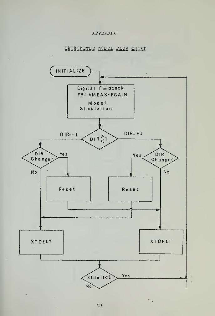
APPENDIX
TACHOMETER MODEL FLOW CHART
c INITIALIZE>iDigital Feedback
FB= VMEAS*FGAIN
ModelSimulation
87


Tach o Pulsea rr ived,
get PERIOD
Store
Write
Reset
IN CR
PLOT
END
Reduce INCRDo same Stepagain
No
Yes j
c a 1 c u late!
V M EASetc
No
88


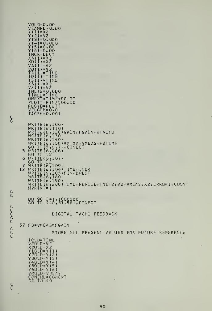
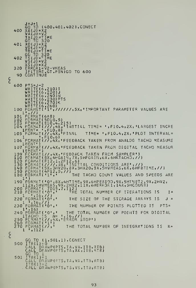
COMPUTER PROGRAM
CC FORTRAN SIMULATION OF DIGITAL TACHOMETERC ANALOG, DIGITAL AND SAMPLER FEEDBACKC SAMPLE PROGRAM INCLUDEDCCccC TACHO PARAMETERSC RT TACHOMETER DISC RADIUSC TACRES TACHOMETER RESOLUTIONC KTACHO NUM8ER OF TACHO PULSES PER INCHC DR DISTANCE BETWEEN TACHO PULSESC TACRV NUMBER OF TACHO PULSES PER RADIANSC TACSH ERROR IN INITIAL TACHO POSITIONC NCLCCK NUMBER OF CLOCKPULSES COUNTEDC COUNT ACTUAL COUNT OF TACHO MARKERSC LCOUNT LAST COUNTC RCOUNT SECOND LAST COUNTC DIR DIRECTION OF VELOCITY
Cc
IMPLICIT REAL*8( A-H,Q-Z)EQUIVALENCE (T I T L E , RT B ( 5 ) )
REAL*8 LCTIME, INCR, KTACHO, T ITLE ( 12
J
REAL *4 RTB<28)/28*0.0/,SINTEGERS IT3< 12 ) / 12*0/ , PTS , S WI TCH, COUNT , COUNT 1
INTEGER *4 RCOUNT , CONECTDIMENSION TA(600 ) , Tu( oOO ) , X A< 60 ) , XD ( 60 ) , V A( 600
)
DIMENSION ""5(600) ,XS(600) , VS ( 600 ) , VO ( 60 )
DIMENSION Y(10),F{10)DATA ITB(2),ITB(3),ITB(4),ITB(5)/0,9,4, 1/DATA ITB(6) , ITB(8)/1, 1/DATA TACSH,RT,LCTIME/0.75D0, l.D0,0.D0/DATA POLE1,POLE2/100. DO, 1000.00/
CcC INITIALIZE VARIABLES AND PARAMETERSCC
READ (5, 10 2) GAIN, FGAI N , VBI AS, OSCF , DELTREAD! 5, 101, END=999) TITLEREAD(5, 102) TACRES, DELAY, FIN, DPLOTREAD(5, 102) TIME,V2,X2,VMEASREAD(5, 103 ) RTB(1 i, CONECT, SWITCHJ = l
K = lN = l
NT =
TACRV=TACRES/6. 2831 85308KTACHO=TACRV/RTDR=1.D0/KTACH0W=6.28315D0*FREQXBIAS=VBIAS*TIMEDIR=1.D0CCNC\T= <50.D0+X2+XBIAS)*KTACH0+TACSHUCOUNT=O.D0CGUNT=IDINT(CONCNTILCOUNT=COUNTR COUNT- 10PERIOD=0.0D0LCTIME=0.000ERR0^1=O.ODOVDCT=0. DO
89

cc
cc
ccccc
ccc
VOLD=O.DOVSAMPL=O.DOY(1)=X2Y(2J=V2Y(3)=0. ODOY(4)=O.ODOY(5)=O.DOY(6)=0. DOINCR=DELTXA(1)=X2XD(1)=X2VA( 1)=V2VD( 1)=V2TA(1»=TIMETD(1)=TIMETS(1)=TIMEXS( 1)=X2VS( 1)=V2TNET2=0.0D0TIMED=TIMEDNEXT=TIME+OPLOTPLOTT=F INI/500.00PLOTD=PLCTTVELCCM=0.0TACSH=0.001
WRITE(6WRITE(6WRITE(6WRITE(6WRITEC6WPITE(6GO TO(WR1TE(GG 70WRITE
<
GO TOWRITEi
FGAIN,KTACHO
,100),110),120)GAIN,,130),140), 150)V2,X2,VMEAS,FBTIME,6,7) , CQNECT106)
o
6,
6,107)12
7 WRITE(6,109).2 WRITE(6,I04)TIME, IMCR
WPITE(6,105)FIN,DPLCTWRITE(6,li30)WRUE(6, 190)WRITE(6,200)NPRINT=1
I ME, PERI0D,TiMET2, V2 , VMEAS , X2 , E RROR 1 , CCUN T
Cc
DO 90 I =1,1000000GO TO ( 40,57,58) ,CONECT
DIGITAL TACHO FEEDBACK
>7 FB=VMEAS*FGAIN
STORE ALL PRESENT VALUES FOR FUTURE REFERENCE
TCLD=TIMEV20LD=V2X20LD=X2Y10L0=Y(1)Y20LD=Y(2)Y30LD=Y(3)Y40LD=Y<4)Y50LD=Y(5)Y60LD=Y (6)VMOLD= VMEASCONCNL=CGNCNTGO TO 40
90


ccc
ccccc
SAMPLE AND HOLD FEEDBACK
Cc
ccccccccccccc
cccc
ccc
ccc
58 I F( (TIME-TIMED) .
VSAMPL=V2TIMED=TIME
59 FB=VSAMPL*FGA1N
LT.OELAYIGO TO 59
SECOND ORDER VELOCITY CONTROL , QUADRATIC
40 VELCOM=100.D0PCLE1=189.7D0IF(C0NECT.EQ.1)FB=Y(2)*FGAINTNET2=( VELC0M-FB-YC2) )*GAINF(1)=Y( 2)F(2)=Y( 3)F(3}=TNET2-P0LE1*Y<3)S=RKLDEQ(3,Y,F,TIME,INCR,NT)X2=Y(1)V2=Y(2)IF(S-l.OO) 70,40,300ERROR STOP
70 WRITE(6,250)STOP
300 IFUCONECT.EQ.l ) .0R.<C0NECT.EQ.3) )G0 TO 301
DIGITAL COUNT SIMULATION
CONCMT IS INTEGRATED UMTIL IT INDICATES THATA TACHO PULSE HAS ARR I V ED .COUNT IS THEN IN-CREASED AND THE NUMBER OF COUNTED OSCILLATIONSDETERMINED. CCNCN T IS INITIALLY SET TO A LARGENUMBER TO PREVENT I
NEGATIVE REGION DURINGOM COUNTING Ii\TONEGATIVE VELOCITIES
XBIAS=VBIAS*TIMEC0NCNT= (5O.D0+X2+XBIAS)*KTACH0+TACSHIF(DIR)32,32,31
HECK FOR CHANGE IN DIRECTION, BY COMPARINGHE CALCULATED DISTANCE WITH THE LAST VALUi
31 IF(CCNCNT-C0NCNL)33,33,3432 IF(CCNCNL-C0NCNT)35,35,36
CHANGE OF DIRECTION OCCURRED FROM + TO -
33 UC0UNT=1.D0CCUNT=I DINT(CONCNT+UCCUNT)RCOUNT=LCOUNTLCOUNT=CCUNTVMEAS=O.DODIP =-1. DOGO TO 3 6
CHANGE OF DIRECTION OCCURRED FROM - TO +
35 UCCUNT=O.DOCOUNT=IDINT(CONCNT]RCOUNT=LCOUNTLCOUNT=CGUNTVMEAS=O.DODIR=1.D0
34 XTDLLT-CONCNT-CO'JNTGO TO 37
91


ccccccccccccc
cccc
cccc
ccccc
ccccc
38
307
308
301
302310
TO SEARCH FOP THE CORRECT PULSE TIME, THEDISTANCE TRAVELED IS DETERMINED BY INTEGRATINGIN DECREASING STEPS OF TIME. IF THE CALCULATEDDISTANCE IS LARGER THAN THE DISTANCE BETWEENTACHO PULSES, THE STEP SIZE IS REDUCED, THEPPEVIOUS VALUES ARE RESTORED AND THE INTEGRATION DONE AGAIN. WHEN THE STEP SIZE REACHES10D-8,THE RESULT IS TAKEN AS AN INDICATIONOF A TACHOMETER PULSE, AND THE TIME IT TOOKFOR THE INTEGRATION IS THE PERIOD BETWEEN TWOTACHOMETER PULSES, THE SAMPLING PERIOD.
36 XTDELT=COUNT-CONCNT37 IFCXTDELT.LT. 1. DO) GO TO 301
IFt INCR.LE.10.D-09) GO TO 38
INTEGRATED TOO FAR , RESET VALUES, GET NEWSTEPSIZE AND INTEGRATE AGAIN
TIME=TOLDX2=X20LDV2=V20LDY(1)=Y10LDY(2)=Y20LDY(3)=Y30LDY(4)=Y40LDY(5)=Y50LDY(6)=Y60LDVMEAS=VMOLDCGNCNT=CONCNLINCR=INCR#0.5D0K = K+1GO TO 40
NEXT PULSE HASACCURACY. NOW SPEED
COUNT = I DI NT CCONCNT + UC OUNT
)
C0UNT1= lABS(CCUNT-RCOUNT)RCOUNT=LCOUNTLCOUNT=COUNTPERIOD=TIME-LCTIMELCTIME=TIMENCLOCK=IDINTCPERIOD*OSCF)
THIS CHECK IS ONLYTHE FIRST ARRIVINGSPEED MEASUREMENT.
WITH REASONABLEIS DETERMINED
IMPORTANT ATPULSE CANNOT
STARTUP,BE USED FOR
IFCCCUNT1.NF.2)G0 to 308VM E AS = DR*OSCF/NCLOCK*DIR-XB I AS/TIMEVDOT=(VMEAS-VOLD) /PERIODVCLD=VMEASERR0R1=V2-VMEASN = N+1NPTS=N-2INCRsDELT
END OF TACHO ROUTINE
IFCTIME.LE.DNEXTJGO TO 310DNEXT=DPLOT+DNEXTWRITE(o,200)TIME,PERI0D,TNET2, V2, VMEAS, X2
,
ERROR 1 , COUNTIF(NPRINT.NE.75)GO TO 302WPITl(6,260)NPRINT=0NPRINT=NPRINT+1IFCTIME.LE.PLOTOJGG TO 320 .
PLOTD=PLOTD+PLOTT
92

cc
400
401
402
320
90
600
J=J + 1
GO TO (400,401,402),C0NECTXA( J)=X2VA(J)=V2TA(J)=T IMEGC TC 320XD( J)=X2VD<J)=V2TO(J)=TIMEGO TO 320TS( J)= T IMEVS(J)=V2XS( J)=X2ERR0R1=V2-VMEASIF(TIME.GT.FIN)GQ TO 600CONTINUE
Cc
1
100
101102103104
]
105
106:
107:
109110120130140150130
190'i
200'210
220;
230'i
2401
250'260270
1
1
1
PTS=J-2WRITE16WRITE(6WRITE(6WRITE(6WRITE(6WPIT£(6FORMAT
(
FORMAT
(
FORMAT
(
FCRMAT(FORMAT
(
MENT= •
FORMaT(',
FORMAT
(
MENT«
)
FORMAT(EMENT' )
FCRMAT(FORMAT I
FORMAT(FORMAT
(
FORMAT(FORMAT
(
FORMAT(• )
FORMAT(12X,5HVFORMAT!FORMAT
(
',16,FORMAT
(
',16,/FORMAT
(
•, 16)
FORMAT
(
tach:' i
FORMAT
(
FORMAT
(
FORMAT
(
• ,112)
,210)
I
,220)J,240)N,230)PTS,270)K,260)•1' ,//////,5X,
'
IMPORTANT PARAMETER VALUES ARE
6A8)5D10.5)E10.4,2I5)///,4X,' INITIAL TIME= ',F10.4,2X,,F10.8)//,4X, 'FINAL TIME= «,F10.4,2X,'F10.6)//,4X,« FEEDBACK TAKEN FROM ANALOG
'LARGEST INCRE
PLOT INTERVAL =
TACHO MEASURE
//,4X, 'FEEDBACK TAKEN FROM DIGITAL TACHO MEASUR
//,4X,'FEDBACK TAKEN FROM SAMPLER5X,4HGAIN, 7X,5HFGAIN,6X, 6HKTACH0,F12. 1,2F12.6)////,5X,
'
INITIAL CONDITIONS ARE',5X,3HV20,8X,3HX20,3X,5HVMEAS,6X,64F12.5,//)
« )
//)
//)HFBTIME,//)
THE TACH3 COUNT VALUES AND SPEEDS ARE
•0' ,8X,4HTIME,9X,6HPERI0D,9X,5HTNMEAS,9X,2HX2,llX,t>HERR3Rl, 14X,5HC7D15.7, I 12 )
•0',' the TOTAL NUMBER OF ITER//)•0«,' THE SIZE OF THE STCRAGE/)'0',' THE NUMBER OF POINTS PLC
•0',' THE TOTAL NUMBER OF POINTS N= ',16,//)//,4X, 'ERROR STOP'
)
'1')
//,' THE TOTAL NUMBER OF INTEGRATIONS IS K=
ET2,9X,2HV2,OUNT)
AT IONS IS 1 =
ARRAYS IS J =
TTED IS PTS=
S FOR DIGITAL
GO TO (1,501,1) ,CCNECT500 ITB(1)=0
CALL DRAWP(PTS,TA,VA, ITB,RTB)CALL DPAWP(PTS,TA,XA,ITB,R T B)GC TO 1
501 ITB(1)-1CALL DRAWP(-TS,TA, VA,IT3,RTB)ITBU ) = 2CALL DRAkP(PTS,T3,VS,ITB,RTB)
93


ITB(1)=3CALL DRAWP(PTS, TO , VD , I TB, RT 6
)
REAO(5, 10DTITLEITB(1)=1CALL DRAWP(PTS,TA,XA,ITB t RTB)ITB<1>=2CALL DRAWP(PTS,TS,XS,ITB,RTS)ITB(1)=3CALL DPAWP(PTS,TD,XD, TTB.RTB)GO TO 1
502 ITB(1)=0CALL DRAWP(PTS,TS,XSiITB f RTB)CALL DRAWP(PTS,TS,VS,ITS,RTB)6C TO 1
999 STGPEND
94


BIBLIOGRAPHY
1. Szabados. B. , diCenzo, C. D. and Sinha, N. K. , "HighResolution Precision Digital Tachometer," IEEETrans. Instr. and i'leas. '
. Vol. IM-21, No. 2,p-TTPT=1ire7-may"~79727
1. Szabados, B. , diCenzo, C. D. and Sinha, N. K. ,
"Diqital Measurement of Angular Velocity," Journalof Physics E: Scientific Instruments, Vol. T> , TTo. 6,p~5IT?-55"27 June~T^7T7
3. Tou, J. T. , Digital and Sampled- Data Control Systems,Mac Graw-Hill BooU Company, Inc. , T9~5"9~.
H. Thaler, G. , Design of feedback Systems, Dowden,Hutchinson ana Ross, Inc. ,T573.
5. Monroe, A. J. , Digital Process for Sampled DataSystems, p 5B-75, tfiley, 79"62.~
6. Eagaazini, J. R. and Franklin, G. I. , Sampled data"Control Systems, Mac Graw-Hill Book Company, 7958.
7. Hufnagel- Rp— j
EJune 1959
8. Kuo, B. , Analysis and Synthesis of Sampled^Data ControlSystems, Prenlice Hall, 7953.
95

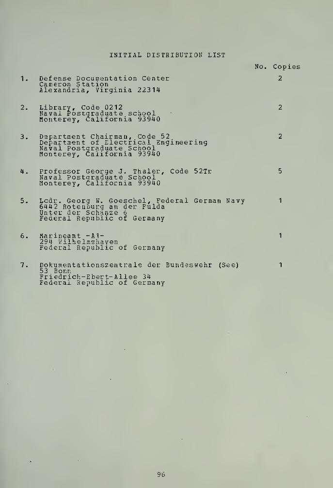
INITIAL DISTRIBUTION LIST
No. Copies
1. Defense Documentation Center 2Cameron StationAlexandria, Virginia 22314
jarv,Naval Postgraduate schoolMonterey, California 93940
3. Department Chairman, Code 52Department of Electrical EngineeringNaval Postgraduate SchoolMonterey, California 93940
4. Professor George J. Thaler, Code 52TrNaval Postgraduate SchoolMonterey, California 93940
5. Lcdr. Georg W. Goeschel, Federal German Navy6442 Rotenourg an der FuldaUnter der Schanze 6Federal Republic of Germany
6. Marineamt -A1-294 WilheimshavenFederal Republic of Germany
7. Dokumentationszentrale der Bundeswehr (See)53 BonnFriedrich-Ebert-Allee 34Federal Republic of Germany
96

6 MAY7S 2282U
Thesis 1556G2G528 Goeschelc.l An engineering study
of a digital tachometerand i ts effects on feed-back control systems.
' - 6 MAY75 2282U
ThesisG528c.l
Goesche
1
An enqineerinq study
of a digital tachometerand its effects on feed
back control systems.
r ro do- L

DUDLEY KNOX LIBRARY
3 2768 00033033 6