Embed Size (px)
Citation preview

NREL is a national laboratory of the US Department of Energy Office of Energy Efficiency amp Renewable Energy Operated by the Alliance for Sustainable Energy LLC This report is available at no cost from the National Renewable Energy Laboratory (NREL) at wwwnrelgovpublications
Contract No DE-AC36-08GO28308
An Energy Signal Tool for Decision Support in Building Energy Systems Gregor P Henze Gregory S Pavlak Anthony R Florita Robert H Dodier and Adam I Hirsch
Technical Report NRELTP-5500-63130 December 2014
NREL is a national laboratory of the US Department of Energy Office of Energy Efficiency amp Renewable Energy Operated by the Alliance for Sustainable Energy LLC This report is available at no cost from the National Renewable Energy Laboratory (NREL) at wwwnrelgovpublications
Contract No DE-AC36-08GO28308
National Renewable Energy Laboratory 15013 Denver West Parkway Golden CO 80401 303-275-3000 bull wwwnrelgov
An Energy Signal Tool for Decision Support in Building Energy Systems Gregor P Henze Gregory S Pavlak Anthony R Florita Robert H Dodier and Adam I Hirsch
Prepared under Task No ARCB1102
Technical Report NRELTP-5500-63130 December 2014
NOTICE
This report was prepared as an account of work sponsored by an agency of the United States government Neither the United States government nor any agency thereof nor any of their employees makes any warranty express or implied or assumes any legal liability or responsibility for the accuracy completeness or usefulness of any information apparatus product or process disclosed or represents that its use would not infringe privately owned rights Reference herein to any specific commercial product process or service by trade name trademark manufacturer or otherwise does not necessarily constitute or imply its endorsement recommendation or favoring by the United States government or any agency thereof The views and opinions of authors expressed herein do not necessarily state or reflect those of the United States government or any agency thereof
This report is available at no cost from the National Renewable Energy Laboratory (NREL) at wwwnrelgovpublications
Available electronically at httpwwwostigovscitech
Available for a processing fee to US Department of Energy and its contractors in paper from
US Department of Energy Office of Scientific and Technical Information PO Box 62 Oak Ridge TN 37831-0062 phone 8655768401 fax 8655765728 email mailtoreportsadonisostigov
Available for sale to the public in paper from
US Department of Commerce National Technical Information Service 5285 Port Royal Road Springfield VA 22161 phone 8005536847 fax 7036056900 email ordersntisfedworldgov online ordering httpwwwntisgovhelpordermethodsaspx
Cover Photos (left to right) photo by Pat Corkery NREL 16416 photo from SunEdison NREL 17423 photo by Pat Corkery NREL 16560 photo by Dennis Schroeder NREL 17613 photo by Dean Armstrong NREL 17436 photo by Pat Corkery NREL 17721
NREL prints on paper that contains recycled content
Executive Summary
This project demonstrates a prototype energy signal tool for operational whole-building and system-level energy use evaluation The purpose of the tool is to provide a summary of building energy use that allows a building operator to quickly distinguish normal and abnormal energy use Toward that end energy use status is displayed as a traffic light which is a visual metaphor for energy use that is either substantially different from expected (red and yellow lights) or approximately the same as expected (green light) Which light to display for a given energy end use is determined by comparing expected to actual energy use As expected energy use is necessarily uncertain we cannot choose the appropriate light with certainty Instead the energy signal tool chooses the light by minimizing the expected cost of displaying the wrong light The expected energy use is represented by a probability distribution Energy use is modeled by a low-order lumped parameter model Uncertainty in energy use is quantified by a Monte Carlo exploration of the influence of model parameters on energy use Distributions over model parameters are updated over time via Bayesrsquo theorem The simulation study was devised to assess whole-building energy signal accuracy in the presence of uncertainty and faults at the submetered level which may lead to tradeoffs at the whole-building level that are not detectable without submetering
iii
Table of Contents
1 Introduction and Motivation 1
2 Literature Review 4
3 Methodology 6 31 Modeling Environment 6
311 Retail Building Simulation Models 6 312 Inverse Gray-Box Building Model for Operational Applications 8 313 Envelope Model Calibration 14 314 HVAC System Modeling 15 315 Overall Retail Building Model Validation 18
32 Uncertainty Quantification 20 321 Model Input Parameter Uncertainty 20 322 Operational and Equipment Faults 21
33 Decision Analysis 24 34 Bayesian Updating 27
4 Results 32 41 Decision Support Case Studies 32
411 Fault-Free Scenario 33 4111 High Energy Consumption Case 33 4112 Medium Energy Consumption Case 33 4113 Low Energy Consumption Case 34
412 Faulted Scenarios 35 4121 High Energy Consumption Case 35 4122 Medium Energy Consumption Case 36 4123 Low Energy Consumption Case 37
42 Bayesian Parameter Updating Case Studies 39 421 High Energy Consumption Case 41 422 Medium Energy Consumption Case 42 423 Low Energy Consumption Case 44
5 Summary and Conclusions 47
Bibliography 48
iv
List of Figures
Figure 1 Energy signal tool flowchart 2
Figure 2 Isometric view of five-zone retail building model 6
Figure 3 Zone plan of five-zone retail building model 7
Figure 4 Twenty-one-parameter thermal RC network 9
Figure 5 Eighteen-parameter thermal RC network 10
Figure 6 Thirteen-parameter thermal RC network 10
Figure 7 Eleven-parameter thermal RC network 10
Figure 8 Eight-parameter thermal RC network 10
Figure 9 Five-parameter thermal RC network 11
Figure 10 Packaged RTU 16
Figure 11 Validation of packaged RTU SA dry bulb temperature 17
Figure 12 Validation of packaged RTU SA humidity ratio 17
Figure 13 Validation of packaged RTU RA dry bulb temperature 17
Figure 14 Validation of packaged RTU RA humidity ratio 17
Figure 15 Validation of packaged RTU electricity demand 18
Figure 16 Validation of packaged RTU gas demand 18
Figure 17 Retail sensible zone load comparison for NSU scenario 19
Figure 18 Retail zone mean air temperature comparison for NSU scenario 19
Figure 19 Retail sensible zone load comparison for precooling scenario 19
Figure 20 Retail zone mean air temperature comparison for precooling scenario 19
Figure 21 Retail HVAC electricity consumption comparison for NSU scenario 20
Figure 22 Retail HVAC electricity consumption comparison for precooling scenario 20
Figure 23 Distributions of whole-building HVAC lighting and plug electricity conshysumption 23
Figure 24 Relationship between deviation thresholds Xlow and Xhigh and state probabilshyity vector PP 25
v
Figure 25 Fault-free high consumption case beginning August 30 (measured consumpshytion data are indicated by diamonds in each figure) 33
Figure 26 Fault-free medium consumption case beginning August 30 (measured conshysumption data are indicated by diamonds in each figure) 34
Figure 27 Fault-free low consumption case beginning August 30 (measured consumpshytion data are indicated by diamonds in each figure) 35
Figure 28 Faulted high consumption case beginning August 30 (measured consumption data are indicated by diamonds in each figure) 36
Figure 29 Faulted medium consumption case beginning August 30 (measured consumpshytion data are indicated by diamonds in each figure) 37
Figure 30 Faulted low consumption case beginning August 30 (measured consumption data are indicated by diamonds in each figure) 38
Figure 31 Example of four buildings managed by a building operator 39
Figure 32 Lighting power density prior (blue) and posterior (red) distributions on September 21 based on past 30 days of high energy consumption Truth value is shown as a green vertical line 41
Figure 33 Equipment power density prior (blue) and posterior (red) distributions on September 21 based on past 30 days of high energy consumption Truth value is shown as a green vertical line 41
Figure 34 Occupant density prior (blue) and posterior (red) distributions on September 21 based on past 30 days of high energy consumption Truth value is shown as a green vertical line 42
Figure 35 DX Coil Rated COP prior (blue) and posterior (red) distributions on September 21 based on past 30 days of high energy consumption Truth value is shown as a green vertical line 42
Figure 36 Gas heating coil efficiency prior (blue) and posterior (red) distributions on September 21 based on past 30 days of high energy consumption Truth value is shown as a green vertical line 42
Figure 37 Lighting power density prior (blue) and posterior (red) distributions on September 21 based on past 30 days of medium energy consumption Truth value is shown as a green vertical line 43
Figure 38 Equipment power density prior (blue) and posterior (red) distributions on September 21 based on past 30 days of medium energy consumption Truth value is shown as a green vertical line 43
Figure 39 Occupant density prior (blue) and posterior (red) distributions on September 21 based on past 30 days of medium energy consumption Truth value is shown as a green vertical line 43
vi
Figure 40 DX Coil Rated COP prior (blue) and posterior (red) distributions on September 21 based on past 30 days of medium energy consumption Truth value is shown as a green vertical line 43
Figure 41 Gas heating coil efficiency prior (blue) and posterior (red) distributions on September 21 based on past 30 days of medium energy consumption Truth value is shown as a green vertical line 44
Figure 42 Lighting power density prior (blue) and posterior (red) distributions on September 21 based on past 30 days of low energy consumption Truth value is shown as a green vertical line 45
Figure 43 Equipment power density prior (blue) and posterior (red) distributions on September 21 based on past 30 days of low energy consumption Truth value is shown as a green vertical line 45
Figure 44 Occupant density prior (blue) and posterior (red) distributions on September 21 based on past 30 days of low energy consumption Truth value is shown as a green vertical line 45
Figure 45 DX Coil Rated COP prior (blue) and posterior (red) distributions on September 21 based on past 30 days of low energy consumption Truth value is shown as a green vertical line 45
Figure 46 Gas heating coil efficiency prior (blue) and posterior (red) distributions on September 21 based on past 30 days of low energy consumption Truth value is shown as a green vertical line 46
List of Tables
Table 1 Selected EnergyPlus Model Details 7
Table 2 Model complexity results 12
Table 3 Calibrated Five-Parameter Network RC Parameters 15
Table 4 Retail Building Use Parameters 21
Table 5 Retail Building HVAC Parameters 21
Table 6 Fault Ranges 22
Table 7 Summary Statistics of Conditional Distributions of Whole-Building HVAC Lighting and Plug Electricity Consumption in [] in [MWha] 23
Table 8 Decision Analysis State and Action 26
Table 9 Building Model Truth Parameters 41
vii
Nomenclature
Pa action vector aopt optimal action
ABCD state space model matrices C opaque building shell thermal capacitance
Cc roof thermal capacitance Cc1 external node roof thermal capacitance Cc2 internal node roof thermal capacitance
Ce exterior wall thermal capacitance Ce1 external node exterior wall thermal capacitance Ce2 internal node exterior wall thermal capacitance Cf floor thermal capacitance
Cf 1 external node floor thermal capacitance Cf 2 internal node floor thermal capacitance
Ci internal thermal capacitance Ci1 node 1 internal thermal capacitance Ci2 node 2 internal thermal capacitance Cp air thermal capacitance Cz zone thermal capacitance
CM zone air capacitance multiplier COP coefficient of performance
D measured data DX direct expansion
ek transfer function heat gain history coefficient E(x) expected value of x
Emeas measured predicted energy consumption Emod model-predicted energy consumption
E0low lower threshold of low deviation E1low upper threshold of low deviation E0high lower threshold of high deviation E1high upper threshold of high deviation
EQP equipment G central green light action
GM internal gain multiplier h f g heat of vaporization of water
HVAC heating ventilation and air conditioning i action index j state index
K cost matrix (decision analysis) or knowledge (inference) LTG lighting mair mass of air in the zone
viii
m M
min f mSA ML MH
NSU n PP p
qocclat QepQgc
Qgrc Qgre
Qgr+solw Qin f
Qsolc Qsole Qsolw
Qsh Qzs
Qrom r
R1 R2 R3 Rc
Rc1 Rc2 Rc3
Re Re1 Re2 Re3 R f
R f 1 R f 2 R f 3
Ri Ri1 Ri2
transfer function heat gain history order model output infiltration mass flow rate supply air mass flow rate much lower state much higher state nighttime setup number of past inputs state probability vector probability occupant latent gains surrogate or measured sensible zone load convective portion of internal gains (lighting occupants and equipment) radiative fraction of internal gains applied to ceiling surface radiative fraction of internal gains applied to vertical wall surface radiative portion of internal gains and solar radiation through glazing infiltration heat gain solar radiation transmitted through opaque ceilingroof surfaces solar radiation transmitted through opaque vertical exterior surfaces solar radiation transmitted through glazing sensible convective heat gain to zone air sensible zone load reduced-order model predicted sensible zone load number of elements in the input vector u combined heat transfer coefficient to opaque shell mass node conduction coefficient between mass and internal surface node convectionradiation coefficient bw surface and zone air temperature nodes roof thermal resistance roof combined external convection and radiation coefficient roof conduction resistance roof internal combined convection and radiation coefficient exterior wall thermal resistance combined external convection and radiation coefficient exterior wall conduction resistance exterior wall internal combined convection and radiation coefficient floor thermal resistance ground conduction coefficient floor conduction resistance floor internal combined convection and radiation coefficient internal partition thermal resistance internal partition combined convection and radiation coefficient internal partition conduction resistance
ix
Ri3 internal partition combined convection and radiation coefficient Rw glazing thermal resistance RA return air RH upper red light action RL lower red light action
ROM reduced-order model RTU rooftop unit
S similar state SA supply air SH somewhat higher state
SHGC solar heat gain coefficient SL somewhat lower state
S transfer function input coefficient matrix t time or time index
Ta outdoor air temperature Tc ceiling node temperature
Tc1 external roof node temperature Tc2 internal roof node temperature
Te exterior wall node temperature Te1 external exterior wall node temperature Te2 internal exterior wall node temperature Tf floor node temperature
Tf 1 external floor node temperature Tf 2 internal floor node temperature
Tg ground temperature Ti internal partition temperature
Tm opaque building shell thermal temperature Ts (pseudo) internal surface temperature Tz zone air temperature Tz average zone air temperature over timestep u input variable vector
WBE whole building electricity consumption Wz zone air humidity ratio
WOA outdoor air air humidity ratio WSA supply air humidity ratio
x state variable vector x state variable first derivative vector
Xhigh definition of high level of deviation threshold Xlow definition of low level of deviation threshold
y output variable vector YH upper yellow light action YL lower yellow light action σε measurement noise Δτ time step
x
1 Introduction and Motivation
Stakeholders of assorted interests are increasingly concerned with the energy performance of the built environment Increasing commitment to energy efficiency cost-minimal retrofits and renewable energy integration has coincided with the availability of commercial and open-source building energy simulation engines Model-based approaches have become the norm with enshygineering design accelerating its reliance on software It is hypothesized that beyond building design applications model-based engineering of buildings can be extended to encompass a buildshyingrsquos multi-decade life cycle Of particular interest is the operational energy performance where tradeoffs in comfort and energy consumption can be hidden and the establishment of normal behavior as distinguished from faulted behavior is nontrivial Research interests lie in data-driven models for decision-making processes that are flexible adaptable and can evolve with the engineered system
A balance must be struck between model sophistication and available data One may have scores of utility bill data available but little understanding of an appropriate physically relevant model Or one might have an exceedingly detailed physical model available but its real-world validity is still questionable because calibration has been performed against sparse utility data Pattern recognition or classification can be used to ascertain the validity of a model and the value of data however building applications are in their infancy At the building systems level monitoring-based heating ventilation and air conditioning (HVAC) commissioning (Wang et al 2013) and chiller fault detection (Zhao et al 2013) have shown promise
The interpretation of patterns might be further aided by providing real-time appliance-level power management and occupant feedback for sociotechnical energy conservation (Gulbinas et al 2014) At the whole-building level participation in the smart grid via approaches such as energy storage may entail value-cognizant electricity demand shifting and shaping (Florita et al 2013) the value to the building owner is likely different than that to the electricity grid Data mining and knowledge discovery tasks have the ultimate goal of predictive diagnostics for buildings and their systems and have shown acceptable levels of misclassification in the face of the evolving nonstationary behavior common to buildings (Kiluk 2014) Sector-wide studies include modeling the evolution and refurbishment of the German heating market (for 2050 goals) and its impact on carbon emissions (Bauermann et al 2014)
The goal of the energy signal tool research is to enable owners and operators of commercial buildings to quickly (in a matter of seconds) attain insight into how their buildingsrsquo energy use compares against the likely range of expected energy consumption over a given time period (days weeks months or years) The output of the energy signal tool is a simple traffic light indicator that summarizes energy consumption relative to model-based expectations To find the appropriate value of the indicator the energy signal tool carries out an analysis of building energy use taking uncertainty and misclassification costs into account As illustrated in Figure 1 the energy signal tool process begins with an operational energy model of a building to provide expected energy performance but recognizes that any model only approximates reality
1
Previous research explored how gray-box models are obtained and calibrated from noisy data (Pavlak et al 2014) and results are extended here to include HVAC systems The term operashytional derives from the desire to consider only a few influential variables within the model and to use them in real-time applications while learning from data as they are gathered We believe that simplified operational models are sufficient when coupled to uncertainty analysis and misclassifishycation costs of relatively simple building types such as big box retail Work is currently underway to develop an open-source tool based on the OpenStudio development effort that would allow the decision analysis to be applied to arbitrarily complex multi-zone buildings
Figure 1 Energy signal tool flowchart
2
A Bayesian probabilistic approach was adopted here to update beliefs about uncertainties in light of new data Over time the energy signal tool learns improved assumptions for input parameter uncertainties by incorporating measured building data into a Bayesian inference process Unobshyserved variables are inferred from data and physical modeling The range of all possible values is divided into five exhaustive and mutually exclusive intervals labeled 1ndash5 in the figure which represent predicted energy use that is substantially lower somewhat lower more or less the same somewhat higher and substantially higher than observed The probability that energy use (at either the whole-building or the end-use level) falls into a given range of values is computed as the integral of the energy use probability distribution over that interval User-defined thresholds determine the toolrsquos sensitivity and are driven by the operatorrsquos risk appetite We then applied utility theory to find the most appropriate action given an assumed cost of misclassification of each action (ie each traffic light color) in each state (ie each energy use interval probability) The expected cost of misclassification is the cost matrix multiplied by the probability vector We chose the element of the expected cost that has the lowest value
To illustrate the operation of the energy signal tool we give examples of its output in various energy use scenarios and review Bayesian updates to model parameters
3
2 Literature Review
Most uncertainties in building energy performance are addressed during the design phase The evolution of a given design involves a sequence of decisions by various domain experts and has implications in thermal visual and acoustical performance (De Wit and Augenbroe 2002) Competing objectives such as energy consumption environmental performance and financial costs warrant multi-objective optimization for decision-making (Diakaki et al 2010 2013) Although engineering tradeoffs lead to numerous optimal and near-optimal solutions eg Pareto fronts (Rafiq 2000) early design choices lead to the buildingrsquos ultimate sustainability (Balcomb and Curtner 2000) Confounding the problem is information sharing with conflicting objectives in the collaborative design process (Ugwu et al 2000) However the primary uncertain drivers in the design process include (1) (micro)climate variables (Sun et al 2014) which may not be appropriately captured by typical meteorological data (2) occupancy patterns and dynamics which may be hard to capture with traditional diversity factor approaches (Li et al 2009) and (3) consideration for the existing infrastructure where the building will be constructed which may be far from ideal (Takizawa et al 2000) Judkoff et al (20081983) described the sources of difference between simulation and reality Recent interest lies in sustainable designs with renewable energy systems (Piotr et al 2012) net zero energy buildings (Attia et al 2012) and overall healthy and productive buildings (Choi et al 2009 Zeiler et al 2012)
Energy management or measurement and verification within existing building energy systems must face a plethora of uncertainties including (but not limited to) noisy sensors point measures of distributed phenomena (eg air temperature) and unobserved variables To capture complex nonlinear and multivariable interactions mathematical approaches such as Gaussian processes (Burkhart et al 2014 Heo and Zavala 2012) multi-agent decision-making control strategies (Zhao et al 2010) and Bayesian-calibrated energy models (Heo et al 2011 Neumann et al 2011) have been used Furthermore with the proliferation of wireless sensor networks in smart buildings (De Farias et al 2014) interest in assessing performance has extended beyond energy into mold growth and remediation (Moon and Augenbroe 2008) as well as disaster preparedness and management (Filippoupolitis and Gelenbe 2009 Vinh 2009) for events such as fires (Sanctis et al 2011) earthquakes (Basso et al 2013) and bioterrorist attacks (Thompson and Bank 2010) The literature shows that the need for decision support within operational building settings is vast yet a balance between risk and situational usefulness needs to be attained
Many authors have devised frameworks for decision support in various building energy perforshymance settings Augenbroe et al (2009) described a tool with an investment strategy for energy performance decision-making for existing buildings with viable refurbishments via optimizashytion Kolokotsa et al (2009) analyzed and categorized buildings for specific actions or groups of plans in a methodology for decision support of building energy efficiency and environmental quality including real-time operation and offline decision-making Das et al (2010) considered building maintainability using an analytical hierarchy process to balance budget requirements with performance standards for nine building systems including input from 37 facilities manshyagement experts Gultekin et al (2013) developed a decision support system for guidance in
4
green retrofits to identify key criteria and feasible alternatives Mohseni et al (2013) offered a comprehensive decision-making methodology for condition monitoring to guide building asset managers aiding capital investments and expenditures In a series of papers Lee et al (2013ab 2012) detailed process models for decision support in energy-efficient building projects and campus-scale infrastructures and summarized a workbench for uncertainty quantification respectively Collectively ie taking this series of three papers together a decision support framework was provided
5
3 Methodology
31 Modeling Environment
For prototyping the energy signal tool the simulation study required the validation of the opershyational building energy model as detailed in the following sections In practice a measurement campaign combined with system identification techniques would be required before the energy signal tool is implemented Because of its Bayesian learning approach the process could be automated with a basic knowledge of the modelrsquos structure
311 Retail Building Simulation Models
The US Department of Energyrsquos EnergyPlus standalone retail reference building (Crawley et al 2001 Deru et al 2010) post-1980 construction was used as a relatively simple first application for prototyping and testing the energy signal tool An isometric view of the original five-zone retail building is shown in Figure 2 along with a plan view of model zoning shown in Figure 3 One zone is dedicated to the entry vestibule two slender zones to the left and right of the vestibule have glazing and are assumed to be affected by solar gains a very large core retail zone occupies about 90 of the floor area Finally a loading and storage zone covers the back of the store Selected model details are highlighted in Table 1 This five-zone EnergyPlus model was used to generate simulated operational data for use in developing the reduced-order building energy models described in the following subsections Surrogate data were preferred here over real measurements so that latent variables could be controlled in the experimental study
Figure 2 Isometric view of five-zone retail building model
6
Figure 3 Zone plan of five-zone retail building model
Table 1 Selected EnergyPlus Model Details
Property Value Units Vintage 1980 year Volume 13984 m3
Conditioned floor area 2294 m2
Bldg avg U-value (no film excluding floor) 0418 W mminus2 Kminus1
Ext wall U-value (no film) 0621 W mminus2 Kminus1
Roof U-value (no film) 0314 W mminus2 Kminus1
Floor U-value (no film) 12904 W mminus2 Kminus1
Internal thermal capacitance 450 MJ Kminus1
Internal thermal capacitance per floor area 1962 kJ Kminus1 mminus2
Infiltration 101 ACH Glazing fraction 7 Glazing U-factor 3354 W mminus2 Kminus1
Glazing solar heat gain coefficient 0385 fraction Lighting power density 323 W mminus2
Equipment power density 523 W mminus2
Occupant density 711 m2person HVAC system CV-DX -
7
312 Inverse Gray-Box Building Model for Operational Applications
The inverse gray-box modeling approach developed for this work is largely based on methods described by Braun and Chaturvedi (Braun and Chaturvedi 2002 Chaturvedi et al 2000) For the application presented in this work it is important to be able to predict transient cooling and heating requirements for the building using inverse models that are trained using on-site data Inverse models for transient building loads range from purely empirical or black-box models to purely physical or white-box models Generally black-box (eg neural network) models require a significant amount of training data and may not always reflect the actual physical beshyhavior whereas white-box (eg finite difference) models require specification of many physical parameters Braun and Chaturvedi introduced a hybrid or gray-box modeling approach that uses a transfer function with parameters that are constrained to satisfy a simple physical repshyresentation for energy flows in the building structure A robust method was also presented for training parameters of the constrained model wherein (1) initial values of bounds on physical parameters are estimated from a rough building description (2) better estimates are obtained using a global direct search algorithm and (3) optimal parameters are identified using a nonlinear regression algorithm They found that 1 to 2 weeks of data are sufficient to train a model so that it can accurately predict transient cooling or heating requirements
Previous to the work by (Braun and Chaturvedi 2002 Chaturvedi et al 2000) (Judkoff et al 2000 Subbarao 1988ab Subbarao et al 1988 1985) developed a modeling scheme consisting of several lumped parameters with direct correspondence to reality and correspondence to a detailed model The model used in combination with field data enabled empirical determination of the input parameters thereby reducing model uncertainty
Inverse gray-box models may be based on the approximation of heat transfer mechanisms by an analogous electrical lumped resistance-capacitance network This approximation creates a flexible structure that allows the modeler to choose the appropriate level of abstraction Model complexity can range from representing entire systems with a few parameters to modeling each heat transfer surface with numerous parameters Depending on the model structure and complexshyity parameters can approximate the physical characteristics of the system Model parameters are then identified through a training period with measured data
Figure 4 shows the 21-parameter thermal network representations that by Braun and Chaturvedi (2002) Chaturvedi et al (2000) found to work well Other forms have been considered in this work and are described below A separate 3R2C network is used to represent external wall ceilshying ground and internal wall heat transfer Looking at the 3R2C network for exterior walls for example Re1 could be thought to represent a combined external convection and radiation coshyefficient Re2 wall conduction resistance and Re3 internal combined convection and radiation coefficient to the zone air node Solar gains from opaque elements are represented by Qsole apshyplied to the external surface nodes (eg Te1 and Tc1) Storage is neglected for glazing elements that are represented by a single resistance Rw Solar gains directly entering the zone through glazshying are distributed among internal partition nodes Ti1 and Ti2 as Qsolw Internal gains are split into convective and radiant fractions Convective fractions are applied directly to the zone air
8
node Tz as Qgc Radiant portions are applied to interior surface nodes Te2 and Tc2 as Qgre and Qgrc respectively (Split is proportional by surface area)
Rc1
Rc2
Rc3
Rf3
Rf2
Rf1
Re1 Re2 Re3 Ri1 Ri2 Ri3
Rw
Ce1 Ce2 Ci1 Ci2
Cf1
Cf2
Cc2
Cc1
Ta Te1 Te2 Tz Ti1 Ti2 Tz
Tg
Tf1
Tf2
Tc2
Tc1
Ta
TaQgc
Qsole Qgre12 Qsolw
12 Qsolw
Qsolc
Qgrc
1
Figure 4 Twenty-one-parameter thermal RC network
When using the inverse gray-box modeling approach described in this work questions naturally arise about the RC network structure that is most appropriate for the modeling task Selecting a very complex model structure results in a difficult parameter estimation task but too simple a model may not appropriately capture the desired dynamics In this research the reduced-order modeling (ROM) environment was developed to allow for model structure flexibility so this question may be investigated As previously mentioned various RC network forms have been considered in this work ranging from five to 21 parameters Because the 21-parameter model was previously introduced discussion will begin with the 18-parameter model (see Figure 5) This model can be considered a subset of the 21-parameter model with the internal surface heat transfer elements simplified to 1R1C This reduced the parameter estimation procedure three parameters and kept most of the structure of the 21-parameter model The 13-parameter model shown in Figure 6 is also a subset of the 21-parameter model with a simplified internal surface node and no ground heat transfer The initial thought for this model is that for small footprint high-rise buildings the ground heat transfer may not be a significant contributor to the overall thermal load Also a subset of the initial 21-parameter network the 11-parameter model (Figure 7) contains the simplified internal surface network as well as a simplified ground heat transfer network and lumped ceiling and exterior wall networks The eight-parameter model shown
9
in Figure 8 further simplifies the 11-parameter model by neglecting ground heat transfer This model contains a 3R2C network for exterior surfaces a glazing resistance and a simplified internal surfacemass network
Rc1
Rc2
Rc3
Rf3
Rf2
Rf1
Re1 Re2 Re3 Ri
Rw
Ce1 Ce2 Ci
Cf1
Cf2
Cc2
Cc1
Ta Te1 Te2 Tz Ti
Tg
Tf1
Tf2
Tc2
Tc1
Ta
TaQgc
Qsole Qgre Qsolw
Qsolc
Qgrc
1
Rc1
Rc2
Rc3
Re1 Re2 Re3 Ri
Rw
Ce1 Ce2 Ci
Cc2
Cc1
Ta Te1 Te2 Tz Ti
Tc2
Tc1
Ta
Ta
Qgc
Qsole Qgre Qsolw
Qsolc
Qgrc
1
Figure 6 Thirteen-parameter thermal RC network
Figure 5 Eighteen-parameter thermal RC network
Re1 Re2 Re3 Ri
Rw
Rf2
Rf1
Ce1 Ce2 Ci
Cf
Ta Te1 Te2 Tz
Tg
Ti
Ta
Tf
Qgc
Qsol Qgr Qsolw
1
Re1 Re2 Re3 Ri
Rw
Ce1 Ce2 Ci
Ta Te1 Te2 Tz Ti
Ta
Qgc
Qsol Qgr Qsolw
A(1 1) =1
Re1Ce1+
1
Re2Ce1
A(1 2) =1
Re2Ce1
A(2 1) =1
Re2Ce2
A(2 2) =1
Re2Ce2+
1
Re3Ce2
A(3 3) =1
RiCi
B(1 2) =1
Re1Ce1
B(1 4) =1
Ce1
B(1 5) =1
Ce1
B(2 1) =1
Re3Ce2
B(2 6) =1
Ce2
B(2 7) =1
Ce2
B(3 1) =1
RiCi
B(3 8) =1
Ci
C(2) =1
Re3
C(3) =1
Ri
D(1) =1
Re3+
1
Ri+
1
Rw
D(2) =1
Rw
D(9) = 1
1
Figure 8 Eight-parameter thermal RC network
Figure 7 Eleven-parameter thermal RC network
10
R1 R2 R3
Rw
C
Ta
Ta
Tm TsTz
Qgr+solw Qgc
A(1 1) =1
C
1
R1+
1
R2+
RwR3
R2R3 + RwR2 + RwR3
B(1 1) =1
C
Rw
R2R3 + RwR2 + RwR3
B(1 2) =1
C
R3
R2R3 + RwR2 + RwR3
B(1 3) =1
R1C
B(1 6) =1
C
RwR3
R2R3 + RwR2 + RwR3
B(1 7) =1
C
R2R3
R2R3 + RwR2 + RwR3
B(1 8) =1
C
R2R3
R2R3 + RwR2 + RwR3
C(1) =Rw
R2R3 + RwR2 + RwR3
D(1) =1
R3+
RwR2
R3 (R2R3 + RwR2 + RwR3)
D(2) =R2
R2R3 + RwR2 + RwR3
D(6) =RwR2
R2R3 + RwR2 + RwR3)
D(7) =RwR2
R2R3 + RwR2 + RwR3)
D(8) =RwR2
R2R3 + RwR2 + RwR3)
D(9) = 1
x = Ax + Bu
y = cx + du
xT = [Tm]
uT = [Tz Ta Tg Qsolc Qsole Qgrc Qgre Qsolw Qgc]
1
Figure 9 Five-parameter thermal RC network
In this work we adopt a five-parameter single-zone model shown in Figure 9 its structure was adapted from the thermal RC network used in the CEN-ISO 13790 Simple Hourly Method load calculations (ISO 2007) Heat transfer and storage of opaque building shell materials are represhysented by R1 R2 and C These elements link the ambient temperature node to a pseudo interior surface temperature node Ts accounting for potential heat storage of the mass materials Glazing heat transfer is represented by a single resistance Rw connecting the ambient temperature node to the surface temperature node because thermal storage of glazing is typically neglected R3 represents a lumped convectionradiation coefficient between the surface temperature node and the zone air temperature node Tz The convective portions of internal gains (lighting occupants and equipment) are applied as a direct heat source to the zone temperature node shown as Qgc and the radiant fraction along with glazing transmitted solar gains Qgr+solw are applied to the surface node
We decided to adopt the five-parameter thermal model after performing a model complexity analysis including all six thermal RC model structures previously presented Each of the six RC networks (five-parameter eight-parameter 11-parameter 13-parameter 18-parameter and 21-parameter) was trained using surrogate data from the five-zone US Department of Energy Stand-alone Retail Reference EnergyPlus model Table 2 summarizes the model performance in terms of root mean square error (RMSE) with respect to a validation dataset and in terms of an objective generalized cross-validation score (GCV) GCV is defined in Equation 31 and essentially weights the mean-squared error based on model complexity (Bracken et al 2010)
Obviously the 11-parameter model is superior to the five-parameter model in terms of RMSE and GCV Visual inspection however proved that the model responses in terms of zone temperature and sensible zone load are virtually identical therefore we chose to adopt the simpler five-parameter model to reduce sample size in the Monte Carlo analyses
N sum (Qromi minus Qepi)
2
GCV = i=1 (31)N-1 minus p 2
N
11
In Equation 31 N represents the total number of data points Qromi is the model predicted zone sensible load Qepi is the surrogate zone load and p is the number of parameters in the model The number of parameters p is equal to the number of RC parameters plus two to account for the internal gain and zone capacitance multipliers that may also be used in model calibration
For the retail building the 18-parameter model produced the lowest RMSE however the 21shyparameter results were inadequate because they should have achieved at least the same score as the lower order model The 11-parameter model produced the lowest GCV which suggests that the additional improvement made by the 18-parameter model was not worth the additional comshyplexity Overall the RMSE values for the retail building are all relatively low further suggesting that all model forms performed well Because satisfactory performance was observed from all models the 5-parameter model was adopted to keep the problem dimensionality low
Table 2 Model complexity results
Retail
Model p N k RMSE GCV
5p 7 504 128 6411 423 times 106
8p 10 504 1024 5338 297 times 106
11p 13 504 8192 3087 100 times 106
13p 15 504 32768 5234 291 times 106
18p 20 504 1048576 3076 103 times 106
21p 23 504 8388608 3192 112 times 106
Slightly suboptimal Should have at least reached 3076 as the 18-parameter retail model
A thermal RC network may be represented by a system of linear first-order differential equations with constant coefficients by performing an energy balance at each node with a storage element This system can be represented in traditional state-space form as
x = Ax + Bu y = Cx + Du
For the five-parameter model adopted in the retail building modeling effort state and input vectors are represented as
xT = [Tm Ts]
uT = [Tz Ta Qgr+solw Qgc]
where Tm is the opaque building shell thermal temperature Ts is the (pseudo) internal surshyface temperature Tz is the zone temperature set point Ta is the ambient external temperature
12
Qgr+solw is the sum of the radiative portion of internal gains and the solar radiation transmitted through glazing and Qgc is the total convective internal gains
The state space equations are then converted to the following heat transfer function form
n m ˙ ST ˙Qsht = sum k utminuskΔτ minus sum ekQshtminuskΔτ (32)
k=0 k=1
where S is a matrix containing input coefficients ek is a vector containing heat gain history coefficients n is the number of past inputs in the calculation and m is the number of past heat gain values in the calculation
The transfer function method is an efficient calculation routine as it relates the sensible heat gains to the space ( Qsh) at time t to the inputs (ut ) of n and heat gains ( Qsht ) of m previous time steps The input weighting coefficients (ST
k ) and zone load coefficients (ek) are the results of the state space to transfer function conversion process described by Seem (Seem 1987)
Performing an energy balance on the zone air node in Equation 33 provides a basis for sensible zone load calculations where Cz is the zone air (or node) capacitance Tz is the zone air tempershyature node Qsht is the zone-sensible heat gain Qin f represents infiltration heat gain and Qzst is the required sensible zone load In effect the RC network model describes the transient heat transfer through opaque and transparent envelope components as well as internal gains from occupants lighting and equipment This network is used to compute the heat gains from these sources to the air node The complete energy balance is provided in Equation 33 including infiltration zone air mass and HVAC heat addition and extraction rates
dTzCz = Qsht + Qzst + Qin f (33)dt
If the differential in Equation 33 is approximated by
dTz Tzt minus TztminusΔasympdt Δτ
it can be rearranged to develop an algebraic inverse transfer function for computing zone temperature predictions from a known zone load shown in Equation 34
r n m sum S0(l)ut (l)+ sum S jutminus jΔτ minus sum e jQshtminus jΔτ + 2
Δ
Cτ z TztminusΔτ + min f Cput (2)+ Qzst
l=2 j=1 j=1Tz = (34)
2 Cz Δτ minus S0(1)+ min f Cp
where r is the number of inputs in input vector u here r = 4 An assumption of this formulashytion is that the heat gains are computed using the average value over the time step so the actual temperature at a given time step can be determined from
Tzt = 2Tzt minus TztminusΔτ
13
An ideal load calculation scheme for a dual set point with a dead band scenario can be described by using the previous equations according to the following procedure
for t = simstart simend do Calculate Qsht using Equation 32 Calculate Qzst to maintain Tz = Tcoolset using Equation 33 (assume cooling first) if Qzst lt 0 (heating required to maintain cooling set point) then
Set Qzst = 0 Compute floating temperature using Equation 34 if Tz lt Theatset then
Recompute Qzst to maintain Tz = Theatset using Equation 33 end
end end
To compute zone humidity the simulation also includes a moisture balance as described in Equation 35
dWZ qocclat mair = min f (WOA minusWZ)+ mSA(WSA minusWz)+ (35)dt h f g
where mair is the mass of air in the zone min f is the mass flow rate of air from infiltration mSA is the supply air (SA) mass flow rate qocclat is the occupant latent gain and h f g is the heat of vaporization of water Wz WOA and WSA are the humidity ratios of the zone outdoor air and SA respectively
313 Envelope Model Calibration
When using the inverse gray-box thermal modeling approach it was necessary to determine the values of R and C parameters that bring the simple model into the closest agreement with the more detailed EnergyPlus model Sum of squares minimization was used to identify model parameters that minimize the RMSE defined by Equation 36 between the ROM predicted (Qrom) and the surrogate or measured ( Qep) sensible zone load
N sum (Qromi minus Qepi)2
i=1J =
(36)N
In this work the two-stage optimization presented by Braun and Chaturvedi (2002) was impleshymented that first performs a direct search over the parameter space to identify a starting point for local refinement The direct search is performed on k uniformly random points located within the bounds of the parameter space The local refinement subject to the same parameter constraints is performed via nonlinear least squares minimization implemented using the MATLAB optimizer
14
lsqnonlin based on trust-region Newton methods The implementation in this environment also allows local refinement to be performed around several good starting points from the direct search For higher complexity models the local optimization can be sensitive to the initial starting point Good results have been found when the 12 best direct search points are given to separately executed least squares algorithms to simultaneously explore several attractive regions Table 3 presents the calibrated parameters for the five-parameter model used throughout this work The zone air capacitance multiplier CM represents furnishing and other mass associated with the air node the internal gain multiplier scales the assumed internal gains from lights and equipment These were considered the nominal parameter values to which uncertainty was applied later in the work
Table 3 Calibrated Five-Parameter Network RC Parameters
Parameter Value Units
R1 R2 R3 Rw C CM
4989 0164 0183 3000 2796 35
(m2K)W (m2K)W (m2K)W (m2K)W kJ(m2K)
-GM 0788 -
314 HVAC System Modeling
For the standalone retail building a typical constant volume packaged rooftop unit (RTU) was modeled Figure 10 provides an overview of the system configuration The RTU model features a temperature- or enthalpy-based outdoor air economizer constant-volume fan single-speed direct expansion (DX) cooling coil and gas heating coil Component models were based on the quasi-steady-state physical formulations used by several mainstream whole-building simulation programs (Brandemuehl et al 1993 DOE 2010) Component models were programmed such that a full air loop can be simulated allowing system air states to be included in a zone moisture balance for computing zone humidity levels
Next we assessed the fidelity of the new HVAC models against the EnergyPlus model Energy-Plus outputs were used as inputs to the new HVAC models to compare with the HVAC system performance only Comparing the EnergyPlus with the HVAC model implementations used in this work Figures 11 and 12 show annual SA temperature and humidity ratio respectively for an annual simulation In Figure 11 the top panel shows the SA temperature for occupied and unoccupied periods To better visualize the information weekly comparison plots are offered for a winter week and a summer week Overall performance is very good during summer conditions Mostly slight temperature deviations were noted during winter periods however early morning startup periods are visible where the ROM shows SA temperature values that are 10 K higher
15
ZONE
SA
Economizer DXCoolingCoil
GasHea9ngCoil
CVFan
RA
OA
Exhaust
Figure 10 Packaged RTU
than the values found by EnergyPlus After further review we discovered that this is an artifact of using average hourly rather than subhourly EnergyPlus outputs as validation data and the fact that the ROM was simulated at hourly time steps
During unoccupied periods the fan and heating coil cycle ran in unison to meet the required heating loads During this operating mode the RTU model reports the SA temperature as the air temperature leaving the heating coil which is near 50Cwhen the coil is operating In the case of the ROM this temperature is reported for the entire hour even though the RTU does not run constantly for the hour Because the EnergyPlus model was simulated at subhourly time steps time intervals existed where they were not necessary for the heating coil and fan to run and thus much lower supply temperatures were reported for some time steps Thus the hourly average SA temperature reported by EnergyPlus was 10 K lower Had detailed (ie subhourly) EnergyPlus outputs been plotted for validation several higher spikes near 50Cwould have been observed along with lower values near 20Cduring the hour
Figures 13 and 14 highlight the calculated return air (RA) temperature and humidity ratio Slight differences in the RA humidity can be observed in the results of the simplified zone moisture balshyance As with SA temperatures this is likely an artifact of using average hourly rather than sub-hourly EnergyPlus outputs as validation data Simple first-order methods were used to implement the moisture balance and may also contribute to numerical differences between the two models However overall the model is a good approximation Figures 15 and 16 show the predicted RTU energy consumption for an annual simulation good results are observed for electricity and gas demand
16
0 1000 2000 3000 4000 5000 6000 7000 8000 9000
20
25
30
35
Time (hours)
Te
mp
era
ture
(C
)
RTU Model ValidationSupply Air Temperature
EnergyPlusSimplified
660 680 700 720 740 76010
20
30
40
50Winter
Time (hours)
Te
mp
era
ture
(C
)
4760 4780 4800 4820 4840 486016
18
20
22
24
26Summer
Time (hours)
0 1000 2000 3000 4000 5000 6000 7000 8000 90000
05
1
15
2x 10
5 Cumulative Temperature (C)
Time (hours)
Te
mp
era
ture
(C
)
RMSE = 143MBE = 012Ann Err = 055
EnergyPlusSimplified
0 1000 2000 3000 4000 5000 6000 7000 8000 9000
5
10
15
x 103
Time (hours)
Hu
mid
ity R
atio
(kg
kg
)
RTU Model ValidationSupply Air Humidity Ratio
EnergyPlusSimplified
660 680 700 720 740 76005
1
15
2
25
3x 10
3 Winter
Time (hours)
Hu
mid
ity R
atio
(kg
kg
)
4760 4780 4800 4820 4840 48600008
001
0012
0014
0016
0018
002Summer
Time (hours)
0 1000 2000 3000 4000 5000 6000 7000 8000 90000
10
20
30
40
50
60
Cumulative Humidity Ratio (kgkg)
Time (hours)
Hu
mid
ity R
atio
(kg
kg
)
RMSE = 000MBE = 000Ann Err = 013
EnergyPlusSimplified
Figure 11 Validation of packaged Figure 12 Validation of pack-RTU SA dry bulb temperature aged RTU SA humidity ratio
0 1000 2000 3000 4000 5000 6000 7000 8000 9000
16
18
20
22
24
Time (hours)
Te
mp
era
ture
(C
)
RTU Model ValidationReturn Air Temperature
660 680 700 720 740 76014
16
18
20
22Winter
Time (hours)
Te
mp
era
ture
(C
)
4760 4780 4800 4820 4840 4860225
23
235
24
245
25
255Summer
Time (hours)
0 1000 2000 3000 4000 5000 6000 7000 8000 90000
05
1
15
2x 10
5 Cumulative Temperature (C)
Time (hours)
Te
mp
era
ture
(C
)
RMSE = 006MBE = 001Ann Err = 004
EnergyPlusSimplified
EnergyPlusSimplified
0 1000 2000 3000 4000 5000 6000 7000 8000 9000
5
10
15
x 103
Time (hours)
Hu
mid
ity R
atio
(kg
kg
)
RTU Model ValidationReturn Air Humidity Ratio
EnergyPlusSimplified
660 680 700 720 740 7600
1
2
3
4x 10
3 Winter
Time (hours)
Hu
mid
ity R
atio
(kg
kg
)
4760 4780 4800 4820 4840 48600008
001
0012
0014
0016
0018
002Summer
Time (hours)
0 1000 2000 3000 4000 5000 6000 7000 8000 90000
10
20
30
40
50
60
Cumulative Humidity Ratio (kgkg)
Time (hours)
Hu
mid
ity R
atio
(kg
kg
)
RMSE = 000MBE = 000Ann Err = 090
EnergyPlusSimplified
Figure 13 Validation of packaged Figure 14 Validation of pack-RTU RA dry bulb temperature aged RTU RA humidity ratio
17
0 1000 2000 3000 4000 5000 6000 7000 8000 90000
1
2
3
4
x 104
Time (hours)
Po
we
r (W
)
RTU Model ValidationHVAC Electric Demand
EnergyPlusSimplified
660 680 700 720 740 7600
2000
4000
6000
8000
10000Winter
Time (hours)
Po
we
r (W
)
4760 4780 4800 4820 4840 48600
1
2
3
4
5x 10
4 Summer
Time (hours)
0 1000 2000 3000 4000 5000 6000 7000 8000 90000
2
4
6
8x 10
7 Cumulative Power (W)
Time (hours)
Po
we
r (W
)
RMSE = 55630MBE = 7180Ann Err = 100
EnergyPlusSimplified
0 1000 2000 3000 4000 5000 6000 7000 8000 90000
05
1
15
2
x 105
Time (hours)
Ga
s D
em
an
d (
W)
RTU Model ValidationHVAC Gas Demand
660 680 700 720 740 7600
05
1
15
2
25x 10
5 Winter
Time (hours)
Ga
s D
em
an
d (
W)
4760 4780 4800 4820 4840 48601
05
0
05
1Summer
Time (hours)
0 1000 2000 3000 4000 5000 6000 7000 8000 90000
05
1
15
2x 10
8 Cumulative Gas Demand (W)
Time (hours)
Ga
s D
em
an
d (
W)
RMSE = 117292MBE = 11713Ann Err = 054
EnergyPlusSimplified
EnergyPlusSimplified
Figure 15 Validation of pack- Figure 16 Validation of aged RTU electricity demand packaged RTU gas demand
315 Overall Retail Building Model Validation
The following results provide a comparison of overall gray-box retail building model perforshymance compared to its five-zone EnergyPlus counterpart That is the RTU HVAC models deshyscribed and validated in Section 314 were coupled to the five-parameter thermal RC network that was developed in Section 312 and calibrated in Section 313 to evaluate the ROM in its entirety To provide better insight into the model performance under various conditions we simshyulated it using typical nighttime setup (NSU) operation during a mild week and a precooling heuristic for a hot week (These are validation time periods ie neither was included in model calibration) Sensible zone load temperature and HVAC electricity consumption are in fairly good agreement for NSU and the precooling scenarios in Figure 17 through 22
18
5760 5780 5800 5820 5840 5860 5880 5900 5920 594080
70
60
50
40
30
20
10
0
10
20
Therm
al L
oad (
kW)
Retail Model ValidationZone Sensible Load NSU
EnergyPlus Simplified
5760 5780 5800 5820 5840 5860 5880 5900 5920 5940
3000
2000
1000
0
Cumulative Thermal Load (kW)
Time (hours)
Therm
al L
oad (
kW)
RMSE = 549MBE = 127Cum Err = 620
EnergyPlus
Simplified
5760 5780 5800 5820 5840 5860 5880 5900 5920 594018
20
22
24
26
28
30
Tem
pera
ture
(C)
Retail Model ValidationZone Temperature minus NSU
setpoint EnergyPlus Simplified
5760 5780 5800 5820 5840 5860 5880 5900 5920 5940
1000
2000
3000
4000
Cumulative Temperature (C)
Time (hours)Te
mpe
ratu
re (C
)
RMSE = 035MBE = 010Cum Err = 046
EnergyPlusSimplified
Figure 17 Retail sensible zone Figure 18 Retail zone mean air temshyload comparison for NSU scenario perature comparison for NSU scenario
4760 4780 4800 4820 4840 4860 4880 4900 4920 4940160
140
120
100
80
60
40
20
0
20
40
Th
erm
al L
oa
d (
kW)
Retail Model ValidationZone Sensible Load Precool
EnergyPlus Simplified
4760 4780 4800 4820 4840 4860 4880 4900 4920 4940
6000
4000
2000
0
Cumulative Thermal Load (kW)
Time (hours)
Th
erm
al L
oa
d (
kW)
RMSE = 588MBE = 211Cum Err = 566
EnergyPlus
Simplified
4760 4780 4800 4820 4840 4860 4880 4900 4920 494016
18
20
22
24
26
28
30
Tem
pera
ture
(C)
Retail Model ValidationZone Temperature minus Precool
setpoint EnergyPlus Simplified
4760 4780 4800 4820 4840 4860 4880 4900 4920 4940
1000
2000
3000
4000
Cumulative Temperature (C)
Time (hours)
Tem
pera
ture
(C)
RMSE = 024MBE = minus004Cum Err = minus019
EnergyPlusSimplified
Figure 19 Retail sensible zone load Figure 20 Retail zone mean air temperature comparison for precooling scenario comparison for precooling scenario
19
5760 5780 5800 5820 5840 5860 5880 5900 5920 59400
10
20
30
40
50
60
70
Energ
y (k
Wh)
Retail Model ValidationHVAC Electric Consumption NSU
EnergyPlus Simplified
5760 5780 5800 5820 5840 5860 5880 5900 5920 59400
1000
2000
3000
4000
Cumulative Energy (kWh)
Time (hours)
Energ
y (k
Wh)
RMSE = 494MBE = 074Cum Err = 347
EnergyPlusSimplified
4760 4780 4800 4820 4840 4860 4880 4900 4920 49400
20
40
60
80
100
120
Energ
y (k
Wh)
Retail Model ValidationHVAC Electric Consumption Precool
EnergyPlus Simplified
4760 4780 4800 4820 4840 4860 4880 4900 4920 49400
2000
4000
6000
Cumulative Energy (kWh)
Time (hours)
Energ
y (k
Wh)
RMSE = 649MBE = 004Cum Err = 011
EnergyPlusSimplified
Figure 21 Retail HVAC electricity con- Figure 22 Retail HVAC electricity consumpshysumption comparison for NSU scenario tion comparison for precooling scenario
32 Uncertainty Quantification
To illustrate the capabilities of the energy signal tool we adopted the five-parameter envelope (single-zone) ROM its parameters were identified from hourly surrogate training data derived from an EnergyPlus simulation of a five-zone retail building near the Chicago Midway Airport This model has five parameters for the building shell however 20 parameters are required for the building its use and HVAC systems each parameter is considered to be uncertain
321 Model Input Parameter Uncertainty
Input parameter distributions are characterized in this work using Gaussian distributions faults are modeled with triangular distributions although any other probability distribution may be selected In this work uncertainties are known varieties that are correctly quantified by an energy analyst using input distributions of choice faults are effects of unobserved uncertainties that affect the measured building performance but not the modeled predictions
The chosen distributions represent the best available knowledge of each uncertain model paramshyeter Input parameters are distributed around a mean that equals the nominal parameter value found from the parameter estimation process that has resulted in the validated ROM presented above A standard deviation of 10 of the mean is adopted for the uncertain input parameters
Adopting the five-parameter ROM 11 parameters are associated with the building shell and use and an additional nine parameters are associated with the HVAC system The seven nominal
20
building envelope parameters are shown in Table 3 the four use parameters are shown in Table 4 and the nine nominal HVAC-related model parameters are shown in Table 5
Table 4 Retail Building Use Parameters
Parameter Value Units
Lighting power density 3230 Wm2
Equipment power density 523 Wm2
Occupant density 71 m2per Infiltration flow rate 39 m3s
Table 5 Retail Building HVAC Parameters
Parameter Value Units
Supply fan efficiency 57 Maximum supply fan airflow 135 m3s Supply fan pressure rise 883 Pa DX coil rated capacity 319 kW DX coil rated sensible heat ratio 70 DX coil rated coefficient of performance (COP) 32 shyDX coil rated air mass flow rate 160 kgs Gas heating coil-rated capacity 457 kW Gas heating coil efficiency 80
To demonstrate the tool five of the 20 input parameters are considered uncertain lighting power density equipment power density occupant density DX coil-rated COP and gas heating coil efficiency The remaining 15 input parameters are taken at their nominal values In reality most of these 20 parameters would be uncertain at different levels of uncertainty
322 Operational and Equipment Faults
In spite of an energy analystrsquos best intentions and a belief that the model accurately reflects the building with all uncertainties undetected faults may affect building performance In this work a fault differs from a parameter uncertainty in that it is present without the knowledge of the energy analyst or building operator ie it is unobserved yet still affects the measured conditional distributions of building energy end use
We chose an additional six model parameters to represent such a faulted state Tehse are modeled by triangular distributions which may be asymmetrical The outdoor air fractionrsquos nominal value is 245 but may vary from 0 to 100 The airside economizer high limit temperature is nominally 28C but can vary between 12 and 40C Essentially at very low values of the
21
high limit temperature the economizer is disabled at high values the economizer operation is not overridden Heating and cooling temperature set points may differ from their assumed values with a random offset from -15 to +15 K Moreover the internal gains schedules may be expanded by up to 3 hours or contracted by up to 3 hours from the nominal building operation schedule Finally the schedules for internal gains from lighting and equipment may be shifted by up to 4 hours in each direction ie to earlier and later onsets Because the environment uses hourly time steps the schedule contractionexpansion and shift are rounded to the nearest full hour For the fault-free scenario the six fault parameters are kept at their nominal values For the faulted case all six fault parameters are randomly perturbed concurrently ie a very wide range of fault combinations is explored
Table 6 Fault Ranges
Parameter Nominal Minimum Maximum Units
Outdoor air fraction 245 0 100 Airside economizer high limit Cooling temperature set point Heating temperature set point Internal gains contractionexpansion Internal gains shift
28 228 217 10
800 am to 600 pm
12 -15 -15 -3 -4
40 +15 +15 + 3 + 4
C C C h h
Random sampling of 10000 annual samples for each case is presented here Because parameter combinations randomly drawn from the input distributions described above may lead to infeashysible model configurations for which no solution can be computed only valid model results are retained The sample rejection was put in place to deal with parameter combinations that cause simulation errors such as non-convergence and subsequent crashes Crashes are most often obshyserved when randomly sampling a wide range of HVAC equipment-rated parameters because the random sampling may not always produce physically consistent rated conditions Thus we expect that the wider the input parameter distributions the more frequently invalid model results are generated In the fault-free scenario 9994 of all samples were valid (six of 10000 failed) in the faulted scenario 9988 of all samples were valid (12 of 10000 failed)
The resultant conditional distribution of whole-building HVAC lighting (LTG) and plug elecshytricity EQP consumption is shown in Figure 23 Table 7 shows pertinent statistics of the same in units of [MWha] In the figure and table whole-building electricity (WBE) please define and add to nomenclature is the sum of HVAC LTG and miscellaneous electric loads EQP For fault-free and faulted cases the table shows the mean 10th 50th (median) and 90th percentiles along with the deterministic mean without consideration of any parameter uncertainty
It is evident that the uncertainty associated with the five selected parameters only slightly affects the mean but strongly affects the variance in the whole-building and submetered end uses The central 80 of the WBE consumption can be found within -7 and +8 from the determinisshytic mean in the fault-free case and within -24 and +20 from the deterministic mean in the
22
faulted case The influence of faults is stronger in the HVAC and LTG end uses compared to the EQP end use Given the dominance of HVAC and LTG end uses on whole-building consumption WBE faults strongly affect WBE as well Above all faults widen the energy distributions
100 200 300 400 500 600 7000
0005
001
0015
002
Prob
abilit
y
Whole Building Electric (MWh)50 100 150 200 250
0
002
004
006
008
Prob
abilit
y
HVAC Electric (MWh)
50 100 150 200 250 300 350 400 4500
0005
001
0015
002
Prob
abilit
y
Light Electric (MWh)10 20 30 40 50 60 70 80
0
002
004
006
008
01
Prob
abilit
y
Plug Electric (MWh)
FaultminusFreeFaulted
Figure 23 Distributions of whole-building HVAC lighting and plug electricity consumption
Table 7 Summary Statistics of Conditional Distributions of Whole-Building HVAC Lighting and Plug Electricity Consumption in [] in [MWha]
Percentile End-Use Case Mean 10th 50th 90th
WBE Deterministic 4163 Fault-free 100 93 100 108 Faulted 99 76 99 120
HVAC deterministic 1565 Fault-free 100 96 100 105 Faulted 96 79 97 112
LTG deterministic 2158 Fault-free 100 87 100 113 Faulted 100 71 99 130
EQP deterministic 441 Fault-free 100 87 100 113 Faulted 100 78 100 123
23
33 Decision Analysis
Comparing monitored data against a probable range of expected energy use is more insightful than comparing against a single number because it allows a building owner to assess the urgency of corrective actions that need to be taken If the measured energy use lies at the edge of the probable range of expected values given all the uncertainties in the model inputs the owner can be very confident that an issue requires attention In this work a decision-making tool was developed based on the probability distribution of model predictions to determine the expected utility of a range of available decisions suggesting the one that maximizes the expected utility The tool takes on the form of a modified traffic light with red yellow and green lights We adopted the perspective that a red light is shown both for high levels of overconsumption and high levels of underconsumption because a building consuming significantly less energy than expected may indicate an operational problem as significant as a building consuming too much A yellow signal is similarly used for cases of mild overconsumption and mild underconsumption A green light is reserved for measured building energy consumption that is in line with model expectations
As a first step a distribution of the model-predicted energy consumption (called Emod) was generated using Monte Carlo simulation as described in Section 32
Second the cases falling on the 5th median and 95th percentiles of the modeled energy distrishybutions were selected to represent low medium and high estimates of actual measured energy consumption (called Emeas) for fault-free and faulted scenarios The decision analysis compared the distribution of model-predicted energy consumption with Emeas to determine appropriate actions thus to illustrate the decision tool these three values of Emeas were taken from the samshypled distributions When physically implemented the measured energy consumption would be determined directly from building metering data
Third boundaries were computed from the measured energy consumption to define meaningful ranges of low and high levels of deviation in energy consumption Beginning with a low level of deviation let us define E0low such that it is Xlow percent below Emeas and E1low such that it is Xlow percent above Emeas
E0low = Emeas(1 minus Xlow)
E1low = Emeas(1 + Xlow)
Similarly for a high level of deviation letrsquos define E0high such that it is Xhigh percent below Emeas and E1high such that it is Xhigh percent above Emeas
E0high = Emeas(1 minus Xhigh)
E1high = Emeas(1 + Xhigh)
Of course Xlow lt Xhigh and we arbitrarily define Xlow to be 5 and Xhigh to be 10 ie a small deviation around the metered end use is plusmn5 and a large deviation plusmn10 It would be easy to adopt different values for Xlow and Xhigh for each building energy end use depending on its
24
temporal variability Once we have a conditional probability distribution of expected energy consumptions in hand we can make various kinds of statements Here we desire to report that the actual energy use is much higher somewhat higher similar somewhat lower or much lower than anticipated We further want to assign costs to making correct and incorrect statements and report the statement that has lowest expected cost
Fourth the empirical cumulative distribution of expected energy consumption was used to find the cumulative probabilities for the anticipated energy consumption to be below E0high (called P1) between E0high and E0low (called P2) between E0low and E1low (called P3) between E1low and E1high (called P4) and above E1high (called P5) Together these probabilities form the state probability vector PP = (P1P2P3P4P5)
T as shown in Figure 24
Figure 24 Relationship between deviation threshshyolds Xlow and Xhigh and state probability vector PP
Fifth we define a cost function K where cost is a function of state and action with a finite numshyber of states and a finite number of actions Therefore this cost function can be represented as a matrix Let us agree that there is one row per action and one column per state K(i j) ie cost of action i in state j Let action i = 1 display the lower red light (RL) on the modified traffic signal action i = 2 the lower yellow (YL) signal i = 3 a green (G) signal action i = 4 the upper yellow (YH) signal and finally i = 5 be displaying the upper red (RH) light Let j = 1 be the state that the model predicts a much lower (ML) energy consumption j = 2 a somewhat lower (SL) energy consumption j = 3 about the same (S) j = 4 a somewhat higher (SH) energy consumption and j = 5 a much higher (MH) energy consumption than the actual building Action vector Pa has thus five elements
25
Table 8 Decision Analysis State and Action
State j Anticipated Model Energy
Action i Much Lower Somewhat Lower Similar Somewhat Higher Much higher
Lower red Lower yellow Central green Upper yellow Upper red
K(RLML) K(YLML) K(GML)
K(YHML) K(RHML)
K(RLSL) K(YLSL) K(GSL)
K(YHSL) K(RHSL)
K(RLS) K(YLS) K(GS)
K(YHS) K(RHS)
K(RLSH) K(YLSH) K(GSH)
K(YHSH) K(RHSH)
K(RLMH) K(YLMH) K(GMH)
K(YHMH) K(RHMH)
An advantage of the presented decision analysis tool lies in its ability to individually set the costs of actions given certain states Here we make reasonable but somewhat arbitrary assumptions on the values of the cost matrix elements Showing an RL light when the model predicts ML energy consumption is assumed to have a cost of 4 (strong false negative lost savings opportunity) when the model predicts an SL energy consumption a cost of 3 (false negative) when the model predicts a similar energy consumption a cost of 2 (weak false negative) when the model predicts an SH energy consumption a cost of 1 (weak false negative) and finally when the model predicts MH energy consumption a cost of 0 (correct identification) Showing an RH light when the model predicts ML energy consumption is assumed to have a cost of 0 (correct identification) when the model predicts an SL energy consumption a cost of 1 (weak false positive) when the model predicts a similar energy consumption a cost of 2 (weak false positive) when the model predicts an SH energy consumption a cost of 3 (false positive) and finally when the model predicts MH energy consumption a cost of 4 (strong false positive unnecessary alarm) Similar arguments can be made for the remaining signals of a lower yellow (YL) a green and an upper yellow (YH) light and we yield the following cost matrix
⎡ K(RLML) K(RLSL) K(RLS) K(RLSH) K(RLMH)
⎤
K =
⎢⎢⎢⎢⎣
K(Y LML) K(GML)
K(Y HML) K(RHML)
K(Y LSL) K(GSL)
K(Y HSL) K(RHSL)
K(Y LS) K(GS)
K(Y HS) K(RHS)
K(Y LSH) K(GSH)
K(Y HSH) K(RHSH)
K(Y LMH) K(GMH)
K(Y HMH) K(RHMH)
⎥⎥⎥⎥⎦
⎡4 3 2 1 0
⎤
=
⎢⎢⎢⎢⎣
3 2 1 0
2 1 0 1
1 0 1 2
0 1 2 3
1 2 3 4
⎥⎥⎥⎥⎦ (37)
The expected cost vector for each action is found by multiplying the cost matrix K with the probability vector PP
E(Pa) = K middot PP
26
⎡ E (RL)
⎤ ⎡ K(RLML) K(RLSL) K(RLS) K(RL SH) K(RLMH)
⎤⎡P1⎤
E (Y L) K(Y LML) K(Y LSL) K(Y LS) K(Y LSH) K(Y LMH) P2⎢ ⎥ ⎢ ⎥⎢ ⎥⎢E (G)
⎥= ⎢
K(G ML) K(GSL) K(GS) K(GSH) K(GMH) ⎥⎢
P3⎥⎢ ⎥ ⎢ ⎥⎢ ⎥⎢
E (Y H)⎥ ⎢
K(Y HML) K(Y H SL) K(Y HS) K(Y HSH) K(Y HMH)⎥⎢
P4⎥⎣ ⎦ ⎣ ⎦⎣ ⎦
E (RH) K(RHML) K(RH SL) K(RHS) K(RHSH) K(RHMH) P5 ⎡ K(RLML)P1 + K(RLSL)P2 + K(RLS)P3 + K(RLSH)P4 + K(RLMH)P5
⎤
K(Y LML)P1 + K(Y LSL)P2 + K(Y LS)P3 + K(Y LSH)P4 + K(Y L MH)P5⎢ ⎥
= K(GML)P1 + K(GSL)P2 + K(GS)P3 + K(GSH)P4 + K(GMH)P5 (38)⎢⎢ ⎥⎥⎢
K(Y HML)P1 + K(Y HSL)P2 + K(Y H S)P3 + K(Y HSH)P4 + K(Y HMH)P5⎥⎣ ⎦
K(RHML)P1 + K(RHSL)P2 + K(RH S)P3 + K(RHSH)P4 + K(RHMH)P5
As suggested by utility theory the last step is to select the best action aopt in the face of uncershytainty ie activate that light which minimizes the expected cost
aopt = argminE(Pa)i
34 Bayesian Updating
Thus far the distributions of the uncertain model parameters were assumed to be Gaussian with a standard deviation equal to a fixed fraction of the parameter mean here 10 The choice of these distributions was made somewhat arbitrarily before any operational data was available from the actual building performance and termed before data because of its consideration prior to observation We believe that building performance measurements collected over an extended time period (ie after data) can be used to infer improved input parameter distributions by applying probability theory in general and Bayesrsquo theorem in particular See Jaynes (Jaynes 2003) for full development of Bayesian probability A brief explanation is provided below for information pertinent to this research
High-dimensional integrals associated with problems in computational physics lead to the develshyopment of Markov Chain Monte Carlo algorithms which can efficiently sample from probability distributions by exploiting the Markov property This has led to the explosion of Bayesian techshyniques with the Metropolis Algorithm as the breakthrough approach (named as one of the top 10 algorithms of the 20th century) (Cipra 2000) A probabilistic perspective not only provides insight into the relationship between sets of model parameters revealing tradeoffs and compenshysating interactions but also lends itself to a continuous model uncertainty quantification and tuning where the posterior distribution of an initial parameter estimate can be used as the prior for a subsequent parameter estimation update once new building performance data have been collected
Dodier used Bayesian (belief) networks for whole-building energy diagnostics (Dodier and Kreishyder 1999 Dodier et al 1998) Lauret et al (2006) demonstrated improvements over traditional parameter estimation methods by applying Bayesrsquo theorem to determine better estimates of conshyvection coefficients for a radiant barrier roof system model More recently Booth et al (2012)
27
used London housing stock models for hierarchical modeling with considerations of internal heating set points fraction of space heating air leakage heating system COP window U-value and window-to-wall ratio
In this work the Bayesian inference of uncertain model parameters relies on the extension of a previously developed technique (Neumann et al 2011) It has benefits over traditional methods because prior knowledge of the system can be directly incorporated into the estimation task and methods for addressing sensor noise are inherent to the Bayesian approach The inference can essentially be thought of as fitting a joint probability distribution to a measured dataset Specifishycally conditional probabilities are related through the product rule to derive Bayesrsquo theorem and allow consideration of before data and after data states of knowledge The prior probability distribution is updated with any measured data to form the posterior probability distribution which represents the state of knowledge in any inference task We propose a periodic process where model input parameter distributions are updated daily weekly monthly or for a similar period of interest As new measurements become available data effectively shape the distribution of expected building energy use according to the information gleaned from a combination of prior knowledge and sensor data uncertainty is still present but should decrease with additional data and understanding of the relationships among variables
The probability of parameter set Θ given measured data D and knowledge of the system K can be written as posterior probability p(Θ|DK) Bayesrsquo theorem then allows the conditional probability p(Θ|DK) to be computed from p(Θ|K) p(D|ΘK) and p(D|K) as shown in Equation 39
p(D|ΘK)p(Θ|DK) = p(Θ|K) (39)
p(D|K)
where p(Θ|K) represents prior knowledge about parameter values p(D|ΘK) represents the likeshylihood of observing the measured dataset D given a particular parameter set Θ and knowledge of the system K and p(D|K) is the probability of observing the dataset Ignoring the reference to system knowledge K the relation can be written in alternate form where the numerator reshymains the product of likelihood and prior and the denominator is a normalization factor so that posterior probabilities sum to unity
p(Θ)p(D|Θ)p(Θ|D) = (310)
sum p(Θi)p(D|Θi) i
Assuming random Gaussian noise about a measured datum Di the likelihood of an observation can be determined from its location within the normal distribution with standard deviation σε this is not in nomenclature centered at micro equal to the measured datum
p(Di|Θ) = radic 1
exp(minus(Di minus Mi)
2 ) (311)
σε 2π 2σε2
where Mi is the model output given the parameter set Θ
28
Further assuming independent errors the likelihood is that the entire dataset is simply the prodshyuct of the likelihoods of all individual points The assumption is likely valid for common HVAC sensors (eg temperature probes) but correlated errors could be handled with a slightly different formulation that is indicative of a fault model Measurement errors are often correlated because of for example hysteresis error or linearity error If such correlated errors are of concern a Bayesian (or other probabilistic) method may be used that can accommodate correlated measureshyments This work nonetheless assumes uncorrelated energy consumption measurements thus it ignores autocorrelation of errors which is estimated to be small For the dynamics and time range considered in this problem model structure is considered more important with respect to data fit than noise correlation From this model assumption we derive the easily computable likelihood function given by Equation 312
The likelihood function is maximized when the exponential term is minimized which occurs as the modeled data approach the measured (or surrogate) data When uniform priors are used with Equation 312 in a Bayesian calibration context the most likely parameters are equivalent to those that would be found using a least squares approach because the exponential term in Equation 312 is essentially the sum of squared errors (Pavlak et al 2014)
minus1 n
1 2p(D|Θ) = radic n exp sum (Di minus Mi) (312)
2σ2-σε 2π ε i=1
Evaluating Equation 312 directly can pose numerical issues because a small range of σε values results in a large range of likelihoods Double precision computing environments are typically capable of evaluating floating point numbers on the order of 10minus308 to 10308 This means that when using 3 weeks of hourly data (ie n = 504) σε must approximately be in the range of [0115] Values outside this range will cause the likelihood (and consequently the posterior) to evaluate to Inf NaN or 0 regardless of the time series fit These numerical issues can be alleviated by computing the natural logarithm of the posterior rather than the posterior directly (Lauret et al 2006 Sivia and Skilling 2006)
To compute the natural log of the posterior first the log of both sides of Equation 310 is taken ⎛ ⎞
p(Θ)p(D|Θ)ln(p(Θ|D)) = ln (313)⎝
sum p(Θi)p(D|Θi)⎠
i
The right-hand side of Equation 313 can be separated using logarithm product and quotient rules
ln(p(Θ|D)) = ln(p(Θ)) + ln(p(D|Θ)) minus ln sum p(Θi)p(D|Θi) (314)
i
29
The log-likelihood term of Equation 314
n1 minus1 2ln(p(D|Θ)) = ln radic n exp sum (Di minus Mi) (315) -σε 2π 2σε
2i=1
can be further simplified by applying product and quotient rules as shown in Equations 316 and 317 respectively
n1 minus1 2ln (p(D|Θ)) = ln radic n + ln exp sum (Di minus Mi) (316) -σε 2π 2σε
2i=1
radic nminus1 2ln(p(D|Θ)) = ln(1) minus ln ((
σε 2π
)n)+ ln exp sum (Di minus Mi) (317)
2σ2ε i=1
With ln(1) = 0 and the power rule can be applied to the middle term of the right-hand side The last term of the right-hand side simplifies because of to logarithmic identity to produce Equation 318
radic nminus1ln(p(D|Θ)) = minusn ln
(σε 2π
)+ sum (Di minus Mi)
2 (318)2σ2
ε i=1
Recombining the simplified log-likelihood of Equation 318 with the log-posterior equation of Equation 314 yields
radic n1 2ln(p(Θ|D)) = ln(p(Θ)) minus n ln(
σε 2π
)minus sum (Di minus Mi) (319)
2σ2ε i=1
minus ln sum p(Θi)p(D|Θi) i
The last term of the right-hand side of Equation 319 is ultimately a constant number subtracted from each individual ln(p(Θi)p(D|Θi)) value Because the value of this constant term does not impact the shape or relative information of the posterior it could be thought of as an arbitrary constant C
radic n1 2ln(p(Θ|D)) = ln(p(Θ)) minus n ln(
σε 2π
)minus sum (Di minus Mi) +C (320)
2σ2ε i=1
The constant term can be moved to the left-hand side of the equation producing Equation 321
radic n1 2ln(p(Θ|D)) minusC = ln(p(Θ)) minus n ln(
σε 2π
)minus sum (Di minus Mi) (321)
2σ2ε i=1
30
Because the objective is to avoid numerical underflow or overflow prescribing
C = max radic
ln(p(Θ)) minus n ln(
σε 2π
) minus
1 n
sum 2(Di minus Mi) (322)2σε
2i=1
shifts all points so that the maximum is 0 A maximum value of 0 in the ln space ensures that all values will be mapped to the interval [01] when taking the exponential After taking exponenshytials the values can be scaled by a constant so that probabilities sum to unity
The σε value is a noise term with physical interpretation Here there are three energy signals of interest HVAC lighting and equipmentndashall electrical terms with the error associated with minor fluctuations not incorporated in the physical model As previously stated prescribing an appropriate σε is necessary to prevent underflow or overflow which causes the inference task to crash from numerical issues The most appropriate σε value can be found by maximum a posteriori (MAP) estimation MAP is used to obtain a point estimate of σε by placing a prior distribution over σε and finding the maximum posterior mode according to the empirical data Because the HVAC lighting and equipment energy signals are considered independent in this study the MAP estimate of σε HVAC σε LT G and σε EQP were performed separately with a uniform prior on each σε set between 0 and 15 of the magnitude of the full individual signals
With the appropriate and optimal σε set for each signal it was then possible to calculate the probability of observing various energy signals as a function of the uncertainty parameters Because the signals are considered independent the joint probability of the building state is a product of the individual probabilities
p =prodpi = pHVAC pLT G pEQP (323) i
With the joint posterior probability distribution available from the equation above it was then possible to sample from the posterior directly or marginalize over all parameters not of interest and form a new prior That is the updating process is prior rarr posterior rarr prior The optimal updating period is a function of the building energy dynamics and available data
31
4 Results
Results are presented that (1) exemplify the decision support aspect of the tool and (2) illustrate the updating of the uncertain model parameters based on measured data
41 Decision Support Case Studies
The decision analysis results presented here are separated into fault-free and faulted scenarios In the fault-free scenario the high medium and low consumption values (surrogates of measured building energy consumption) are drawn from the conditional energy consumption distributions without faults and the decision analysis is based on the same distribution In contrast in the faulted scenario the high medium and low consumption values are drawn from the conditional energy consumption distributions including faults and the decision analysis is based on the distribution excluding faults
The results are shown as a matrix of figures The first row shows the whole-building electricity WBE consumption results for the last year then last month then last week followed by the last day The second row shows the HVAC energy consumption results for the time periods the third row shows the lighting LTG results and lastly the fourth row shows the EQP results Each of the 16 figure panels reveals a box plot1 Larger and smaller values respectively are shown as outliers of the expected energy consumption value for the time period of interest a diamond marker superimposed on the box plot to indicate the surrogate actual consumption value Emeas and on the left margin the energy signal tool with the signal chosen for the resultant cumulative probabilities PP cost matrix C and deviation thresholds Xlow and Xhigh The central green light separates cases of mild (YH) and strong (RH) overconsumption above the green light from the cases of of mild (YL) and strong (RL) underconsumption below the green light The particular traffic signal-inspired design is one of many possible designs chosen for illustration here thus many other valid designs can be conceived Moreover the planned field implementation of this energy signal tool would likely not show the box plots but only the signals Finally if only whole-building energy WBE measurements are available the tool would reveal only the top row of WBE versus the four time periods In contrast when submetering of HVAC LTG and EQP is available the lower three rows would be shown and the top WBE row omitted because it would not offer additional insight
1Box plots shown in this report adopt the common notation that the box occupies the interquartile range (IQR) from the lower (25th percentile) to the upper (75th percentile) The whiskers extend to the minimum and maximum values if these are less than 15 times the IQR below the lower or 15 times the IQR above the upper quartile
32
411 Fault-Free Scenario
4111 High Energy Consumption Case
Beginning on August 30 with the high energy consumption case at the 95th percentile a mild overconsumption is shown for all time scales for WBE and HVAC LTG and EQP show strong overconsumption for all time scales
350
400
450
500
WBEYear
MWh
35
40
45
50
55
WBEMonth
MWh
8
9
10
11
12
WBEWeek
MWh
1100
1200
1300
1400
1500
1600
1700
WBEDay
kWh
140
150
160
170
180
HVACYear
MWh
18
20
22
24
26
28
HVACMonth
MWh
4
45
5
55
6
HVACWeek
MWh
500
550
600
650
700
750
HVACDay
kWh
150
200
250
300
LTGYear
MWh
12
14
16
18
20
22
24
LTGMonth
MWh
3
35
4
45
5
55
LTGWeek
MWh
500
600
700
800
900
LTGDay
kWh
30
35
40
45
50
55
60
EQPYear
MWh
25
3
35
4
45
5
EQPMonth
MWh
06
07
08
09
1
11
EQPWeek
MWh
80
100
120
140
160
EQPDay
kWh
Figure 25 Fault-free high consumption case beginning August 30 (meashysured consumption data are indicated by diamonds in each figure)
4112 Medium Energy Consumption Case
The medium consumption cases for August and February show consistency between WBE HVAC and LTG green lights are shown for all time scales and the EQP consumption is low Because the EQP contribution to the total is small the WBE signal is not swayed to show a low yellow light
33
350
400
450
500
WBEYear
MWh
35
40
45
50
55
WBEMonth
MWh
8
9
10
11
12
WBEWeek
MWh
1100
1200
1300
1400
1500
1600
1700
WBEDay
kWh
140
150
160
170
180
HVACYear
MWh
18
20
22
24
26
28
HVACMonth
MWh
4
45
5
55
6
HVACWeek
MWh
500
550
600
650
700
750
HVACDay
kWh
150
200
250
300
LTGYear
MWh
12
14
16
18
20
22
24
LTGMonth
MWh
3
35
4
45
5
55
LTGWeek
MWh
500
600
700
800
900
LTGDay
kWh
30
35
40
45
50
55
60
EQPYear
MWh
25
3
35
4
45
5
EQPMonth
MWh
06
07
08
09
1
11
EQPWeek
MWh
80
100
120
140
160
EQPDay
kWh
Figure 26 Fault-free medium consumption case beginning August 30 (measured consumption data are indicated by diamonds in each figure)
4113 Low Energy Consumption Case
In the low consumption case it is interesting to note that the WBE signal shows a strong unshyderconsumption (low red) driven by the corresponding LTG signal even though HVAC conshysumption is similar to the model expectation (green) and EQP is only a mild underconsumption This case reveals the importance of submetering Without it it would not have been possible to isolate that LTG causes the warning HVAC could be ignored and EQP could be given less consideration
34
350
400
450
500
WBEYear
MWh
35
40
45
50
55
WBEMonth
MWh
8
9
10
11
12
WBEWeek
MWh
1100
1200
1300
1400
1500
1600
1700
WBEDay
kWh
140
150
160
170
180
HVACYear
MWh
18
20
22
24
26
28
HVACMonth
MWh
4
45
5
55
6
HVACWeek
MWh
500
550
600
650
700
750
HVACDay
kWh
150
200
250
300
LTGYear
MWh
12
14
16
18
20
22
24
LTGMonth
MWh
3
35
4
45
5
55
LTGWeek
MWh
500
600
700
800
900
LTGDay
kWh
30
35
40
45
50
55
60
EQPYear
MWh
25
3
35
4
45
5
EQPMonth
MWh
06
07
08
09
1
11
EQPWeek
MWh
80
100
120
140
160
EQPDay
kWh
Figure 27 Fault-free low consumption case beginning August 30 (meashysured consumption data are indicated by diamonds in each figure)
412 Faulted Scenarios
In the faulted scenarios the three cases are drawn from much wider distributions as shown in Figure 23
4121 High Energy Consumption Case
The high consumption case for August 30 shows consistency between WBE HVAC and LTG RH lights are shown for all time scales and the EQP consumption is close to model expectation However because the EQP contribution to the total is small the WBE signal is not swayed to show a low green light
35
350
400
450
500
WBEYear
MWh
35
40
45
50
55
WBEMonth
MWh
8
9
10
11
12
WBEWeek
MWh
1100
1200
1300
1400
1500
1600
1700
WBEDay
kWh
140
150
160
170
180
HVACYear
MWh
18
20
22
24
26
28
HVACMonth
MWh
4
45
5
55
6
HVACWeek
MWh
500
550
600
650
700
750
HVACDay
kWh
150
200
250
300
LTGYear
MWh
12
14
16
18
20
22
24
LTGMonth
MWh
3
35
4
45
5
55
LTGWeek
MWh
500
600
700
800
900
LTGDay
kWh
30
35
40
45
50
55
60
EQPYear
MWh
25
3
35
4
45
5
EQPMonth
MWh
06
07
08
09
1
11
EQPWeek
MWh
80
100
120
140
160
EQPDay
kWh
Figure 28 Faulted high consumption case beginning August 30 (meashysured consumption data are indicated by diamonds in each figure)
4122 Medium Energy Consumption Case
On an annual basis the medium consumption case leads to the expected green lights On time scales of months and shorter we can observe HVAC mild and strong underconsumption
36
350
400
450
500
WBEYear
MWh
35
40
45
50
55
WBEMonth
MWh
8
9
10
11
12
WBEWeek
MWh
1100
1200
1300
1400
1500
1600
1700
WBEDay
kWh
140
150
160
170
180
HVACYear
MWh
18
20
22
24
26
28
HVACMonth
MWh
4
45
5
55
6
HVACWeek
MWh
500
550
600
650
700
750
HVACDay
kWh
150
200
250
300
LTGYear
MWh
12
14
16
18
20
22
24
LTGMonth
MWh
3
35
4
45
5
55
LTGWeek
MWh
500
600
700
800
900
LTGDay
kWh
30
35
40
45
50
55
60
EQPYear
MWh
25
3
35
4
45
5
EQPMonth
MWh
06
07
08
09
1
11
EQPWeek
MWh
80
100
120
140
160
EQPDay
kWh
Figure 29 Faulted medium consumption case beginning August 30 (measured consumption data are indicated by diamonds in each figure)
4123 Low Energy Consumption Case
The low consumption case at the 5th percentile of the faulted distribution shows a consistent RL light for all end uses and time scales independent of season
37
300
350
400
450
500
WBEYear
MWh
35
40
45
50
55
WBEMonth
MWh
7
8
9
10
11
12
WBEWeek
MWh
1000
1100
1200
1300
1400
1500
1600
1700
WBEDay
kWh
130
140
150
160
170
180
HVACYear
MWh
18
20
22
24
26
28
HVACMonth
MWh
4
45
5
55
6
HVACWeek
MWh
500
550
600
650
700
750
HVACDay
kWh
150
200
250
300
LTGYear
MWh
12
14
16
18
20
22
24
LTGMonth
MWh
3
35
4
45
5
55
LTGWeek
MWh
500
600
700
800
900
LTGDay
kWh
30
35
40
45
50
55
60
EQPYear
MWh
25
3
35
4
45
5
EQPMonth
MWh
06
07
08
09
1
11
EQPWeek
MWh
80
100
120
140
160
EQPDay
kWh
Figure 30 Faulted low consumption case beginning August 30 (meashysured consumption data are indicated by diamonds in each figure)
Finally we present a sample illustration of how such a decision analysis tool would be deployed in the management of distributed commercial buildings Imagine a building operator is responsishyble for the energy-efficient operation of four buildings in a city Building 1 appears to be healthy all end uses show green signals for all four time scales building 2 suffers from overconsumption problems in the HVAC system that manifest themselves in the last day week and month buildshying 3 exhibits underconsumption in LTG especially during the last week which could speak to failed light sources or delamping measures not yet accounted for in the model finally building 4 suffers from multiple symptoms overconsumption in HVAC and EQP and underconsumption in LTG
38
Figure 31 Example of four buildings managed by a building operator
42 Bayesian Parameter Updating Case Studies
Results related to the probabilistic inference and updating of the uncertain model parameters are presented for September 21 at which point measurements over the past 30 days are used to update the five input parameter distributions that are deemed uncertain The high consumption case representing the 95th percentile of the fault-free conditional distributions is used to compute the likelihood functions for HVAC LTG and EQP for each of the nearly 10000 parameter
39
combinations Based on the simplifying assumptions articulated above we can then find the marginal posterior distribution for each selected uncertain parameter Please note that white Gaussian noise with a signal-to-noise ratio of 25 was added to the time series data of the high consumption case to simulate common measurement noise affecting building measurements Recent work by the same authors has shown the Bayesian inference approach to be robust with respect to a wide range of signal-to-noise ratios and noise colors (Pavlak et al 2014)
Table 9 shows the nominal values used to generate the prior input parameter distributions as well as the parameter values associated with the low medium and high cases investigated in this section The latter represent the ground truth values that will be compared to the posterior distributions for each model parameter to determine whether the measured data are used to update our belief of the uncertain parameters in a way that is consistent with the ground truth data
The table shows that several individual parameters appear inconsistent with the case they beshylong to As one example in the low consumption case the DX coil-rated COP is 31 which is below the nominal value One would expect a higher COP to be associated with the low conshysumption case However given the tradeoffs between lighting and equipment power consumption and the efficiency of the cooling equipment the low consumption case at the 5th percentile of 10000 simulation runs was the result of a less efficient RTU with strongly reduced lighting and equipment power densities The median consumption case resulted from a slightly higher lighting power density lower equipment power density lower occupant density and higher RTU COP all relative to the nominal values The high consumption case at the 95th percentile of all cases is characterized by higher lighting equipment and occupancy densities and lower HVAC equipment efficiency In this case of higher consumption the individual parameter values are all consistent with the theme of the case
Later sections discuss that whatever tradeoffs were at play in leading to the low medium and high cases the Bayesian parameter updating process is changing the posterior parameter disshytributions toward the ground truth values that form the basis of the measured (here surrogate) consumption data To that effect each of the following figures 32 to 46 shows the sampled prior distribution of the uncertain parameter as blue bars the sampled posterior distribution as red bars and the ground truth value that formed the basis of the surrogate measured data as a green vertical line
Gas heating efficiency should have no impact on electricity consumption thus increased electricshyity consumption should be independent from gas heating coil efficiency All the figures showing gas heating efficiency distributions illustrate that the gas heating efficiency posterior distribution is being smeared out ie becoming less informative because the evidence used in the likelihood function does not offer any clear clues about how to shape the posterior Although we show the prior and posterior distributions for gas heating efficiency for all three cases the independence of electricity consumption from gas heating efficiency is seen in a widening posterior in each case
40
Table 9 Building Model Truth Parameters
Parameter Nominal Low Medium High Units
Lighting power density 3230 2699 3309 3615 Wm2
Equipment power density 523 492 496 594 Wm2
Occupant density 0141 0149 0137 0151 perm2
DX coil rated COP 320 310 339 294 -Gas heating coil efficiency 80 74 70 77
421 High Energy Consumption Case
Figures 32 through 36 clearly illustrate how the measured data would be harnessed to update our belief about the uncertain parameters Each figure shows the empirical prior distribution as blue bars the empirical posterior distribution is shown as red bars Where the two distributions overlap a darker purple hue appears As stated above in the high energy consumption case all individual building parameter truth values are consistent with the theme of high energy conshysumption Lighting and equipment power density posteriors move to higher values relative to the nominal values that served as the mean of the normal prior distributions and gravitate toward the truth values (green vertical lines) used to generate the surrogate measured data Similarly occupancy densities in people per square meter are also slightly higher and the DX coil-rated COP is significantly lower than the nominal value gravitating toward the truth values Thus the Bayesian inference learns the truth values that form the basis of the measured data
Figure 32 Lighting power density prior (blue) and posterior (red) distributions on
September 21 based on past 30 days of high energy consumption Truth
value is shown as a green vertical line
Figure 33 Equipment power density prior (blue) and posterior (red) distribushytions on September 21 based on past 30 days of high energy consumption Truth value is shown as a green vertical line
41
Figure 34 Occupant density prior (blue) and posterior (red) distributions on
September 21 based on past 30 days of high energy consumption Truth
value is shown as a green vertical line
Figure 35 DX Coil Rated COP prior (blue) and posterior (red) distributions on
September 21 based on past 30 days of high energy consumption Truth
value is shown as a green vertical line
Figure 36 Gas heating coil efficiency prior (blue) and posterior (red) distributions on September 21 based on past 30 days of high energy consumption Truth value is shown as a green vertical line
422 Medium Energy Consumption Case
Figures 37 through 41 show how in the medium consumption case the data reveal the tradeoffs that form the basis of the medium consumption case A slightly higher lighting power density is compensated for by a significantly lower equipment power density because these two have the identical effects of adding convective internal gains to the sensible energy balance paired with slightly higher COPs Occupant density distribution has not materially changed from prior
42
to posterior in the medium consumption case As in the high consumption case the posterior distributions (except for gas heating efficiency as explained above) have moved in the direction of the truth values that form the foundation of the surrogate measured data
Figure 37 Lighting power density prior (blue) and posterior (red) distributions
on September 21 based on past 30 days of medium energy consumption Truth value is shown as a green vertical line
Figure 38 Equipment power density prior (blue) and posterior (red) distributions
on September 21 based on past 30 days of medium energy consumption Truth value is shown as a green vertical line
Figure 39 Occupant density prior (blue) and posterior (red) distributions on
September 21 based on past 30 days of medium energy consumption Truth value is shown as a green vertical line
Figure 40 DX Coil Rated COP prior (blue) and posterior (red) distributions on
September 21 based on past 30 days of medium energy consumption Truth value is shown as a green vertical line
43
Figure 41 Gas heating coil efficiency prior (blue) and posterior (red) distributions on September 21 based on past 30 days of medium
energy consumption Truth value is shown as a green vertical line
423 Low Energy Consumption Case
Figures 42 through 46 again clearly illustrate how the measured data would be harnessed to update our belief about the uncertain parameters In the low consumption case the data suggest significantly lower lighting and equipment power densities although occupant density seems to materially impact the measured data which lead to a virtually unchanged posterior
As shown in Table 9 the truth value of the DX coil-rated COP is slightly lower than the nominal value which is opposite to the theme of lower energy consumption As explained above the slightly inferior COP is more than compensated for by significantly lower lighting and equipment power densities The posterior COP distribution is close2 to the prior but slightly less than it feels like something is missing here suggesting that the Bayesian inference has learned the truth value
As before electricity consumption should not and does not have informative power for gas heating efficiency leaving the posterior smeared out relative to the prior
2A very heuristic visual interpretation of close was used We simply encourage the reader to determine in which direction the posterior distribution mass has been moving to the left to the right or virtually unchanged relative to the prior distribution In particular the point of using such loose language is to avoid comparing the empirical prior and posterior distributions with a more rigorous metric such as the maximum distance of the two cumulative distribution functions as used in the two-sample Kolmogorov-Smirnof test Future work will look into more rigorous metrics to automate the update process The point we wanted to make in this work however is that evidence is collected and used to inform updates of the input parameter distributions
44
Figure 42 Lighting power density prior (blue) and posterior (red) distributions
on September 21 based on past 30 days of low energy consumption Truth value is shown as a green vertical line
Figure 44 Occupant density prior (blue) and posterior (red) distributions on
September 21 based on past 30 days of low energy consumption Truth
value is shown as a green vertical line
Figure 43 Equipment power density prior (blue) and posterior (red) distribushytions on September 21 based on past 30 days of low energy consumption Truth value is shown as a green vertical line
Figure 45 DX Coil Rated COP prior (blue) and posterior (red) distributions
on September 21 based on past 30 days of low energy consumption Truth value is shown as a green vertical line
45
Figure 46 Gas heating coil efficiency prior (blue) and posterior (red) distributions on September 21 based on past 30 days of low
energy consumption Truth value is shown as a green vertical line
46
5 Summary and Conclusions
A prototype energy signal tool was demonstrated for operational whole-building and system-level energy performance assessment The purpose of the tool is to give an assessment that a building operator or other user can quickly comprehend Toward this end the energy signal tool estimates energy use for various end uses from a low-order lumped-parameter model taking into account uncertainty (via a Monte Carlo method) in model parameters and inputs The result of the modelshying phase is a probability distribution over estimated energy use The range of estimated energy use is divided into intervals based on the observed energy use and the probability that energy use is in an interval is computed as the mass of the estimated energy use distribution in that interval An indicator (traffic light color) is chosen to minimize misclassification cost Model parameter distributions are adjusted over time via Bayesian updating
The experimental study investigated whole-building energy signal accuracy in the presence of uncertainty and faults at the submetered level which may lead to tradeoffs at the whole-building level that are not detectable without submetering Submetering of end uses is recommended to avoid confounding underconsumption and overconsumption among various end uses An examshyple of four building energy signal displays is offered to illustrate energy performance features that could be detected by the energy signal tool The Bayesian inference results presented show that observations can be used to periodically update model parameter distributions and that the posterior distributions indeed gravitate toward the ground truth parameter values that formed the basis of the surrogate measured data We presented results for a 30-day learning cycle
Future improvements in the inference process would eliminate the assumptions of temporal independence of subsequent observations of a particular variable and structural independence of multiple observed variables Accounting for covariance among observed variables will help to better attribute observations to individual model parameters
47
Bibliography
Attia S Gratia E Herde AD Hensen JL (2012) ldquoSimulation-based decision support tool for early stages of zero-energy building designrdquo Energy and Buildings 49(0) pp 2 ndash 15
Augenbroe G Castro D Ramkrishnan K (2009) ldquoDecision model for energy performance improvements in existing buildingsrdquo Journal of Engineering Design and Technology 7(1) pp 21 ndash 36
Balcomb J Curtner A (2000) ldquoMulti-criteria decision-making process for buildingsrdquo Energy Conversion Engineering Conference and Exhibit Vol 1 pp 528 ndash 535 Las Vegas NV USA IEEE
Basso N Garavaglia E Sgambi L Imagawa N (2013) Natural hazards vs Decision-making processes in buildings life cycle management New York NY USA CRC Press
Bauermann K Spiecker S Weber C (3 2014) ldquoIndividual decisions and system development Integrating modelling approaches for the heating marketrdquo Applied Energy 116 pp 149ndash158
Booth A Choudhary R Spiegelhalter D (Feb 2012) ldquoHandling uncertainty in housing stock modelsrdquo Building and Environment 48(0) pp 35ndash47
Bracken C Rajagopalan B Prairie J (Mar 2010) ldquoA multisite seasonal ensemble streamflow forecasting techniquerdquo Water Resources Research 46(3) pp 1ndash12 URL httpdoiwileycom1010292009WR007965
Brandemuehl M Shauna G Inger A (1993) ldquoHVAC2 Toolkit Algorithms and Subroutines for Secondary HVAC System Energy Calculationsrdquo ASHRAE Atlanta GA
Braun JE Chaturvedi N (2002) ldquoAn inverse gray-box model for transient building load predictionrdquo HVACampR Research 8(1) pp 73ndash100
Burkhart MC Heo Y Zavala VM (2014) ldquoMeasurement and verification of building systems under uncertain data A Gaussian process modeling approachrdquo Energy and Buildings 75 pp 189 ndash 198
Chaturvedi N Braun J Bernhard R (2000) Analytical Tools for Dynamic Building Conshytrol Implementation of Thermal Storage in Building Mass American Society of Heating Refrigerating and Air-Conditioning Engineers
Choi JH Aziz A Loftness V (2009) ldquoDecision support for improving occupant environmenshytal satisfaction in office buildings The relationship between sub-set of IEQ satisfaction and overall environmental satisfactionrdquo Ninth International Conference of Healthy Buildings p 747 Syracuse NY USA
48
Cipra BA (2000) ldquoThe best of the 20th century Editors name top 10 algorithmsrdquo SIAM news 33(4) pp 1ndash2
Crawley DB Lawrie LK Winkelmann FC Buhl WF Huang YJ Pedersen CO Strand RK Liesen RJ Fisher DE Witte MJ et al (2001) ldquoEnergyPlus creating a new-generation building energy simulation programrdquo Energy and Buildings 33(4) pp 319ndash331
Das S Chew M Poh KL (2010) ldquoMulti-criteria decision analysis in building maintainability using analytical hierarchy processrdquo Construction Management and Economics 28(10) pp 1043 ndash 1056
De Farias C Soares H Pirmez L Delicato F Santos I Carmo LF De Souza J Zomaya A Dohler M (2014) ldquoA control and decision system for smart buildings using wireless sensor and actuator networksrdquo European Transactions on Telecommunications 25(1) pp 120 ndash 135
De Wit S Augenbroe G (2002) ldquoAnalysis of uncertainty in building design evaluations and its implicationsrdquo Energy and Buildings 34(9) pp 951 ndash 958
Deru M Field K Studer D Benne K Griffith B Torcellini P Halverson M Winiarski D Liu B Rosenberg M Huang J Yazdanian M Crawley D (2010) US Department of Energy Commercial Reference Building Models of the National Building Stock Washington DC US Department of Energy Energy Efficiency and Renewable Energy Office of Building Technologies
Diakaki C Grigoroudis E Kabelis N Kolokotsa D Kalaitzakis K Stavrakakis G (2010) ldquoA multi-objective decision model for the improvement of energy efficiency in buildingsrdquo Energy 35(12) pp 5483 ndash 5496
Diakaki C Grigoroudis E Kolokotsa D (2013) ldquoPerformance study of a multi-objective mathematical programming modelling approach for energy decision-making in buildingsrdquo Energy 59 pp 534 ndash 542
Dodier R Kreider J (1999) ldquoWhole Building Energy Diagnosticsrdquo ASHRAE Trans 105(1) pp 579ndash589
Dodier RH Curtiss PS Kreider JF (1998) ldquoSmall-scale on-line diagnostics for an HVAC systemrdquo Transactions-American Society Of Heating Refrigerating And Air Conditioning Engineers 104 pp 530ndash539
DOE U (2010) ldquoEnergyPlus Engineering Referencerdquo The Reference to EnergyPlus Calculashytions URL httpapps1eereenergygovbuildingsenergypluspdfs engineeringreferencepdf
49
Filippoupolitis A Gelenbe E (2009) ldquoA decision support system for disaster management in buildingsrdquo Summer Computer Simulation Conference pp 141 ndash 147 Society for Modeling amp Simulation International
Florita AR Brackney LJ Otanicar TP Robertson J (2013) ldquoClassification of Commercial Building Electrical Demand Profiles for Energy Storage Applicationsrdquo Journal of Solar Energy Engineering 135(3) p 031020
Gulbinas R Jain RK Taylor JE (2014) ldquoBizWatts A modular socio-technical energy management system for empowering commercial building occupants to conserve energyrdquo Applied Energy In-Press
Gultekin P Anumba CJ Leicht RM (2013) ldquoTowards an integrated process model and decision support system for high performance green retrofitsrdquo Architectural Engineering Conference 2013 pp 912 ndash 923 State College PA United states
Heo Y Augenbroe G Choudhary R (2011) ldquoRisk analysis of energy-efficiency projects based on bayesian calibration of building energy modelsrdquo Twelth Conference of International Building Performance Simulation Association pp 2579 ndash 2586 Sydney AUS
Heo Y Zavala VM (2012) ldquoGaussian process modeling for measurement and verification of building energy savingsrdquo Energy and Buildings 53 pp 7 ndash 18
ISO E (2007) ldquo13790 2007rdquo Energy performance of buildings-Calculation of energy use for space heating and cooling
Jaynes ET (2003) Probability theory the logic of science Cambridge university press
Judkoff R Balcomb J Hancock C Barker G Subbarao K (2000) Side-By-Side Thermal Tests of Modular Offices A Validation Study of the STEM Method NREL Report TP-550shy23940 National Renewable Energy Laboratory
Judkoff R Wortman D OrsquoDoherty B Burch J (20081983) Methodology for Validating Building Energy Analysis Simulations NREL Report No TP-550-42059 National Renewable Energy Laboratory Golden CO
Kiluk S (11 2014) ldquoDynamic classification system in large-scale supervision of energy effishyciency in buildingsrdquo Applied Energy 132 pp 1ndash14
Kolokotsa D Diakaki C Grigoroudis E Stavrakakis G Kalaitzakis K (2009) ldquoDecishysion support methodologies on the energy efficiency and energy management in buildingsrdquo Advances in Building Energy Research 3(1) pp 121 ndash 146
Lauret P Miranville F Boyer H Garde F Adelard L (May 2006) ldquoBayesian parameter estimation of convective heat transfer coefficients of a roof-mounted radiant barrier systemrdquo Journal of Solar Energy Engineering 128 pp 213 ndash 225
50
Lee BD Sun Y Augenbroe G Paredis CJ (2013a) ldquoTowards better prediction of building performance A workbench to analyze uncertainty in building simulationrdquo Thirteenth Internashytional Conference of the International Building Performance Simulation Association pp 1231 ndash 1238 Chambery France
Lee SH Augenbroe G Lee JK Zhao F (2013b) ldquoA design methodology for energy infrastructures at the campus scalerdquo Computer-Aided Civil and Infrastructure Engineering 28(10) pp 753 ndash 768
Lee S Liu Y Chunduri S Solnosky RL Messner JI Leicht RM Anumba CJ (2012) ldquoDevelopment of a process model to support integrated design for energy efficient buildingsrdquo International Conference on Computing in Civil Engineering pp 261 ndash 268 Clearwater Beach FL USA
Li Z Heo Y Augenbroe G (2009) ldquoHVAC design informed by organizational simulationrdquo Eleventh International IBPSA Conference pp 2198 ndash 2203 Glasgow UK
Mohseni H Setunge S Zhang GM Wakefield R (2013) ldquoCondition monitoring and condition aggregation for optimised decision making in management of buildingsrdquo Applied Mechanics and Materials 438-439 pp 1719 ndash 1725
Moon HJ Augenbroe G (2008) ldquoEmpowerment of decision-makers in mould remediationrdquo Building Research and Information 36(5) pp 486 ndash 498
Neumann C Jacob D Burhenne S Florita A Burger E Schmidt F (2011) Model-Based Methods for Fault Detection and Optimization in Building Operations (Modellbasierte Methoden fuumlr die Fehlererkennung und Optimierung im Gebaumludebetrieb) Fraunhofer ISE
Pavlak G Florita A Henze G Rajagopalan B (2014) ldquoComparison of Traditional and Bayesian Calibration Techniques for Gray-Box Modelingrdquo Journal of Architectural Engineershying 20(2) p 04013011
Piotr R Laurence B Alison C Ahmed AS (2012) ldquoDecision making aid for selection of renewablesustainable energy systems for buildingsrdquo International Conference on Sustainable Design and Construction pp 306 ndash 313 Kansas City MO USA ASCE
Rafiq M (2000) ldquoImportance of Pareto optimum solutions in making informed decisions in engineering designrdquo Eighth International Conference on Computing in Civil and Building Engineering Vol 2 pp 1325 ndash 1333 Stanford CA USA ASCE
Sanctis GD Fischer K Kohler J Fontana M Faber M (2011) A probabilistic frameshywork for generic fire risk assessment and risk-based decision making in buildings Zurich Switzerland CRC Press
Seem J (1987) Modeling of heat transfer in buildings PhD Thesis University of Wisconsin-Madison
51
Sivia D Skilling J (2006) ldquoParameter estimation IIrdquo Data Analysis A Bayesian Tutorial Chap 3 pp 35 ndash 77 Oxford University Press
Subbarao K (1988a) PSTAR - Primary and Secondary Terms-Analysis and Renormalization A Unified Approach to Building and Energy Simulations and Short-Term Testing A Summary NREL Report TR-254-3347 National Renewable Energy Laboratory
mdashmdashmdash (1988b) PSTAR - Primary and Secondary Terms Analysis and Renormalization A Unified Approach to Building Energy Simulations and Short-Term Monitoring NREL Report TR-254-3175 National Renewable Energy Laboratory
Subbarao K Burch J Hancock C Lekov A Balcomb J (1988) Short-term Energy Monishytoring (STEM) Application of the PSTAR Method to a Residence in Fredericksburg Virginia NREL Report TR-254-3356 National Renewable Energy Laboratory
Subbarao K Mort D Burch J (1985) Short-Term Measurements for the Determination of Envelope Retrofit Performance NREL Report TP-253-2639 National Renewable Energy Laboratory
Sun Y Heo Y Tan M Xie H Jeff Wu C Augenbroe G (2014) ldquoUncertainty quantificashytion of microclimate variables in building energy modelsrdquo Journal of Building Performance Simulation 7(1) pp 17 ndash 32
Takizawa A Kawamura H Tani A (2000) ldquoSimulation of urban system ldquoas it could berdquo by multiagent modelrdquo Eighth International Conference on Computing in Civil and Building Engineering Vol 2 pp 1566 ndash 1573 Stanford CA USA ASCE
Thompson BP Bank LC (2010) ldquoUse of system dynamics as a decision-making tool in building design and operationrdquo Building and Environment 45(4) pp 1006 ndash 1015
Ugwu O Anumba C Newnham L Thorpe A (2000) ldquoAgent-oriented collaborative design of industrial buildingsrdquo Eighth International Conference on Computing in Civil and Building Engineering Vol 1 pp 333 ndash 340 Stanford CA USA ASCE
Vinh A (2009) ldquoComputer-based monitoring for decision support systems and disaster preshyparedness in buildingsrdquo Systemics Cybernetrics and Informatics 7 pp 51ndash56
Wang L Greenberg S Fiegel J Rubalcava A Earni S Pang X Yin R Woodworth S Hernandez-Maldonado J (2 2013) ldquoMonitoring-based HVAC commissioning of an existing office building for energy efficiencyrdquo Applied Energy 102 pp 1382ndash1390
Zeiler W Maaijen R Maassen W (2012) ldquoDecision support for sustainable healthier and more productive buildingsrdquo Tenth International Conference Healthy Buildings pp 1ndash6 Brisbane AUS
52
Zhao P Suryanarayanan S Simoes MG (2010) ldquoAn energy management system for building structures using a multi-agent decision-making control methodologyrdquo Industry Applications Society Annual Meeting pp 1ndash8 Houston TX USA IEEE
Zhao Y Wang S Xiao F (12 2013) ldquoPattern recognition-based chillers fault detection method using Support Vector Data Descriptionrdquo Applied Energy 112 pp 1041ndash1048
53
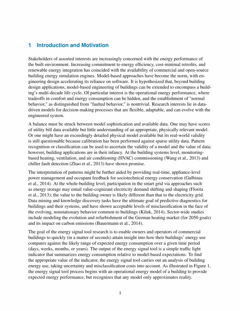
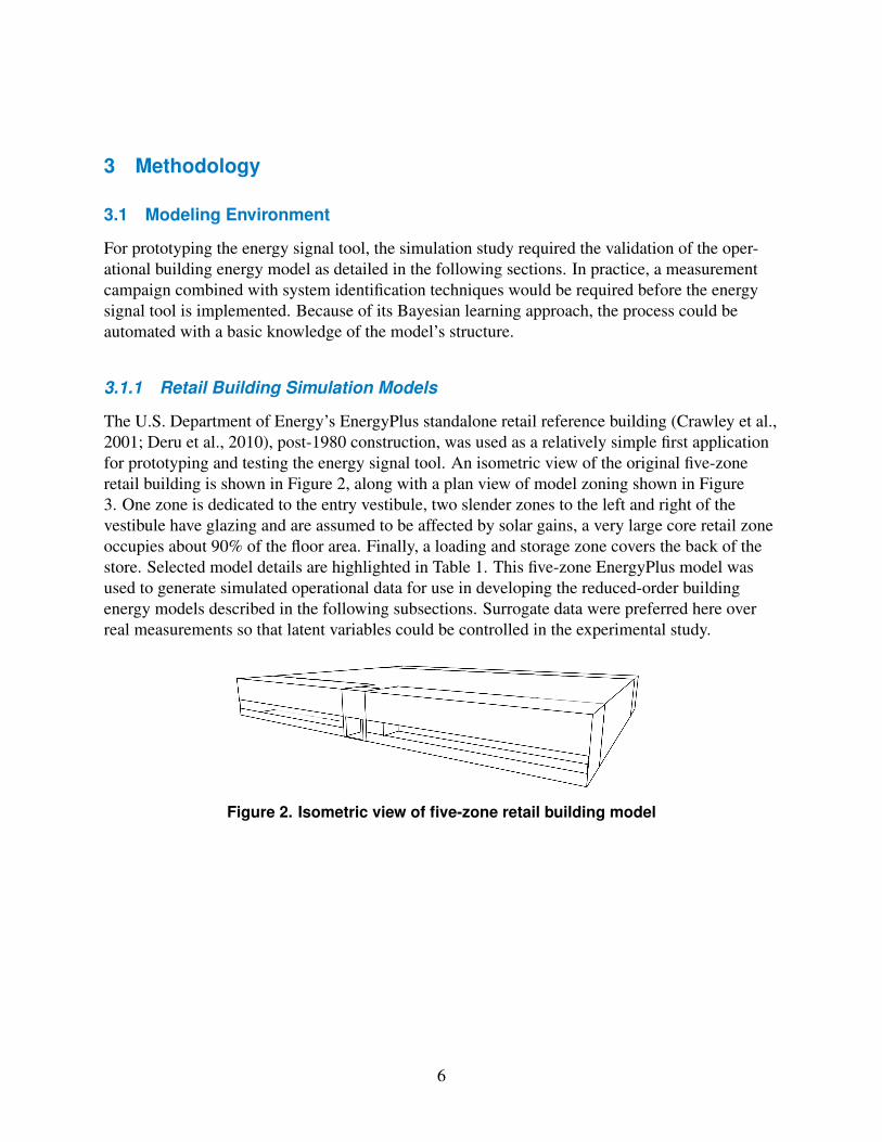
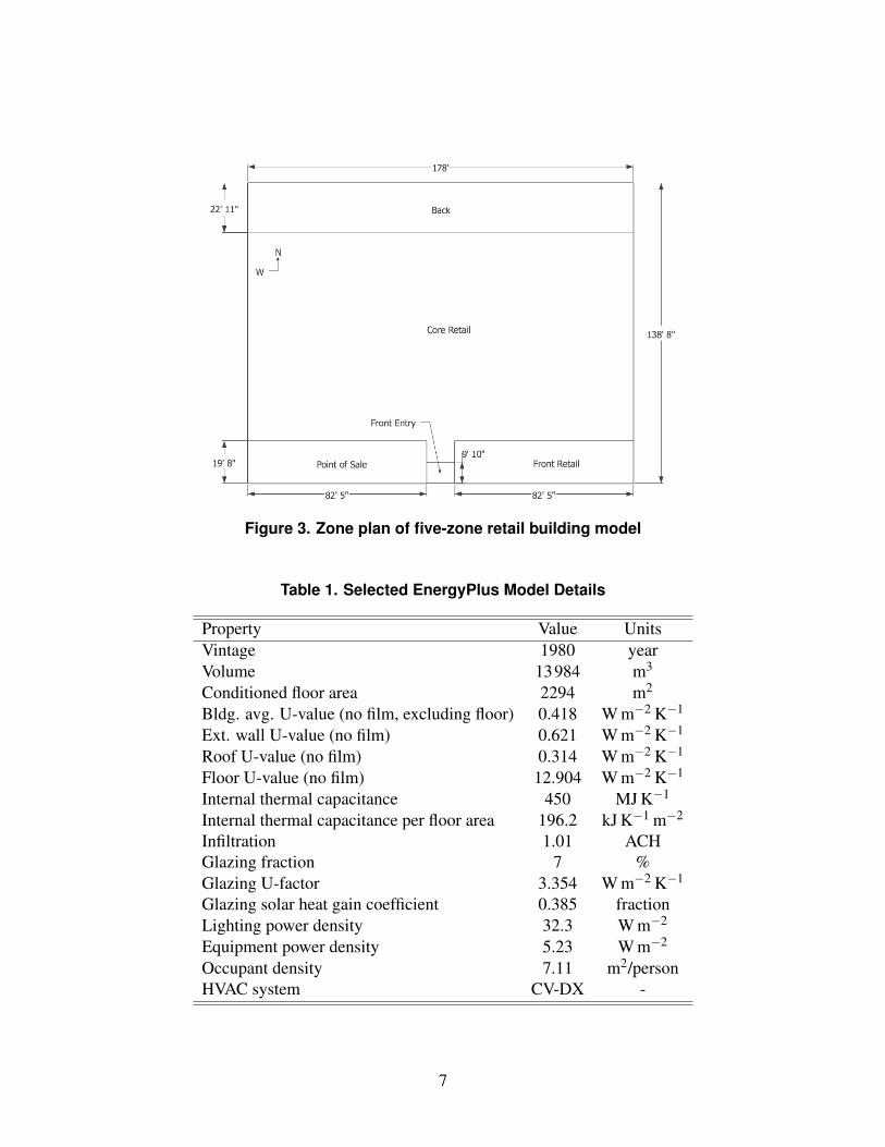
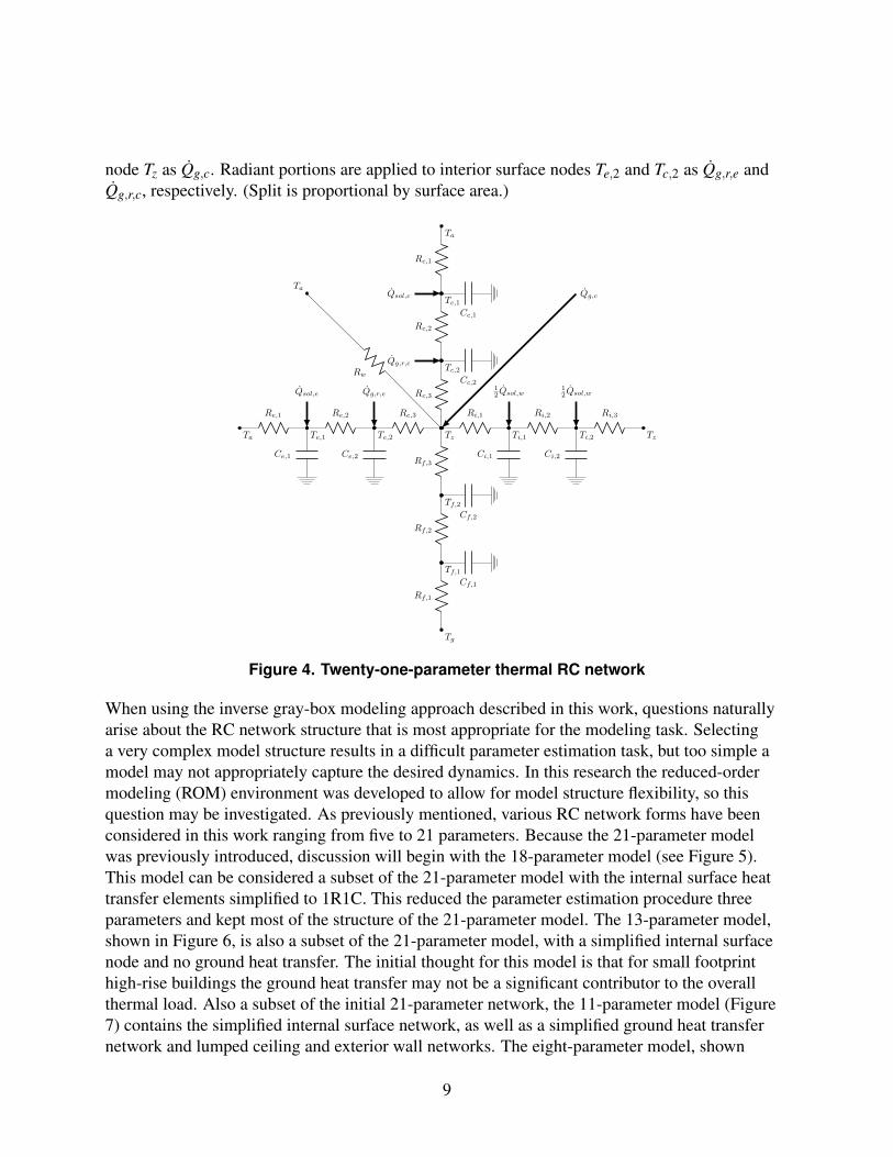
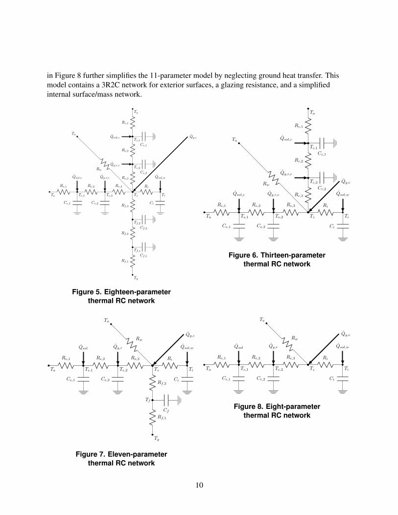
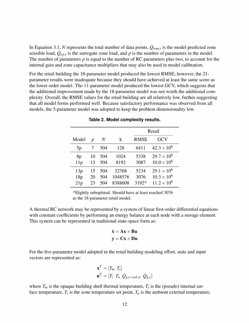
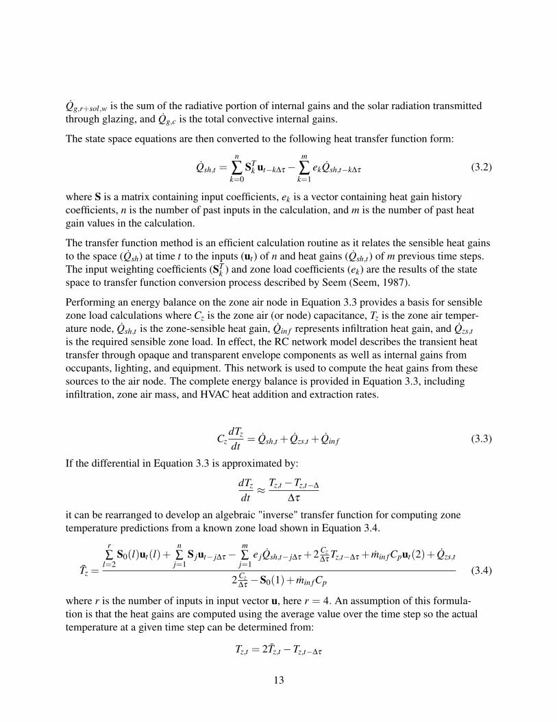
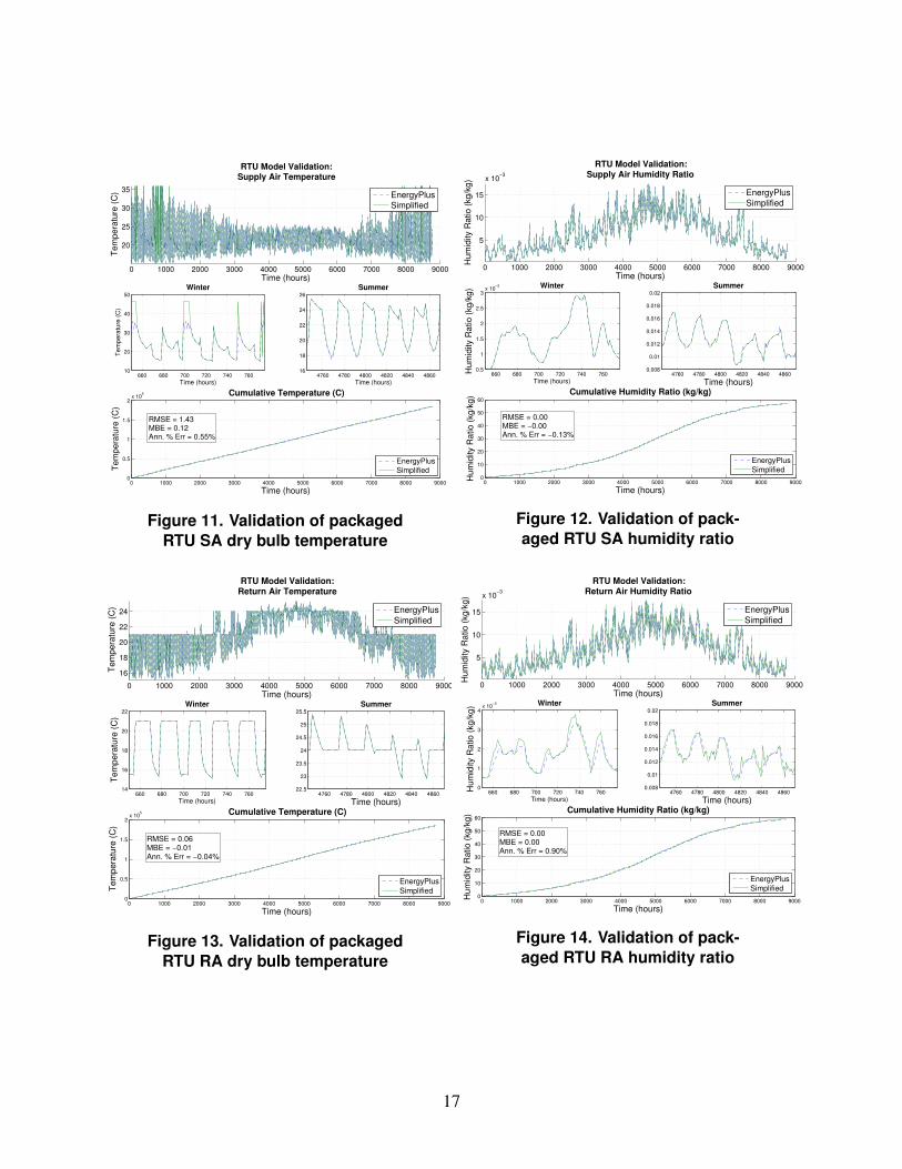
0 1000 2000 3000 4000 5000 6000 7000 8000 9000
20
25
30
35
Time (hours)
Te
mp
era
ture
(C
)
RTU Model ValidationSupply Air Temperature
EnergyPlusSimplified
660 680 700 720 740 76010
20
30
40
50Winter
Time (hours)
Te
mp
era
ture
(C
)
4760 4780 4800 4820 4840 486016
18
20
22
24
26Summer
Time (hours)
0 1000 2000 3000 4000 5000 6000 7000 8000 90000
05
1
15
2x 10
5 Cumulative Temperature (C)
Time (hours)
Te
mp
era
ture
(C
)
RMSE = 143MBE = 012Ann Err = 055
EnergyPlusSimplified
0 1000 2000 3000 4000 5000 6000 7000 8000 9000
5
10
15
x 103
Time (hours)
Hu
mid
ity R
atio
(kg
kg
)
RTU Model ValidationSupply Air Humidity Ratio
EnergyPlusSimplified
660 680 700 720 740 76005
1
15
2
25
3x 10
3 Winter
Time (hours)
Hu
mid
ity R
atio
(kg
kg
)
4760 4780 4800 4820 4840 48600008
001
0012
0014
0016
0018
002Summer
Time (hours)
0 1000 2000 3000 4000 5000 6000 7000 8000 90000
10
20
30
40
50
60
Cumulative Humidity Ratio (kgkg)
Time (hours)
Hu
mid
ity R
atio
(kg
kg
)
RMSE = 000MBE = 000Ann Err = 013
EnergyPlusSimplified
Figure 11 Validation of packaged Figure 12 Validation of pack-RTU SA dry bulb temperature aged RTU SA humidity ratio
0 1000 2000 3000 4000 5000 6000 7000 8000 9000
16
18
20
22
24
Time (hours)
Te
mp
era
ture
(C
)
RTU Model ValidationReturn Air Temperature
660 680 700 720 740 76014
16
18
20
22Winter
Time (hours)
Te
mp
era
ture
(C
)
4760 4780 4800 4820 4840 4860225
23
235
24
245
25
255Summer
Time (hours)
0 1000 2000 3000 4000 5000 6000 7000 8000 90000
05
1
15
2x 10
5 Cumulative Temperature (C)
Time (hours)
Te
mp
era
ture
(C
)
RMSE = 006MBE = 001Ann Err = 004
EnergyPlusSimplified
EnergyPlusSimplified
0 1000 2000 3000 4000 5000 6000 7000 8000 9000
5
10
15
x 103
Time (hours)
Hu
mid
ity R
atio
(kg
kg
)
RTU Model ValidationReturn Air Humidity Ratio
EnergyPlusSimplified
660 680 700 720 740 7600
1
2
3
4x 10
3 Winter
Time (hours)
Hu
mid
ity R
atio
(kg
kg
)
4760 4780 4800 4820 4840 48600008
001
0012
0014
0016
0018
002Summer
Time (hours)
0 1000 2000 3000 4000 5000 6000 7000 8000 90000
10
20
30
40
50
60
Cumulative Humidity Ratio (kgkg)
Time (hours)
Hu
mid
ity R
atio
(kg
kg
)
RMSE = 000MBE = 000Ann Err = 090
EnergyPlusSimplified
Figure 13 Validation of packaged Figure 14 Validation of pack-RTU RA dry bulb temperature aged RTU RA humidity ratio
17
0 1000 2000 3000 4000 5000 6000 7000 8000 90000
1
2
3
4
x 104
Time (hours)
Po
we
r (W
)
RTU Model ValidationHVAC Electric Demand
EnergyPlusSimplified
660 680 700 720 740 7600
2000
4000
6000
8000
10000Winter
Time (hours)
Po
we
r (W
)
4760 4780 4800 4820 4840 48600
1
2
3
4
5x 10
4 Summer
Time (hours)
0 1000 2000 3000 4000 5000 6000 7000 8000 90000
2
4
6
8x 10
7 Cumulative Power (W)
Time (hours)
Po
we
r (W
)
RMSE = 55630MBE = 7180Ann Err = 100
EnergyPlusSimplified
0 1000 2000 3000 4000 5000 6000 7000 8000 90000
05
1
15
2
x 105
Time (hours)
Ga
s D
em
an
d (
W)
RTU Model ValidationHVAC Gas Demand
660 680 700 720 740 7600
05
1
15
2
25x 10
5 Winter
Time (hours)
Ga
s D
em
an
d (
W)
4760 4780 4800 4820 4840 48601
05
0
05
1Summer
Time (hours)
0 1000 2000 3000 4000 5000 6000 7000 8000 90000
05
1
15
2x 10
8 Cumulative Gas Demand (W)
Time (hours)
Ga
s D
em
an
d (
W)
RMSE = 117292MBE = 11713Ann Err = 054
EnergyPlusSimplified
EnergyPlusSimplified
Figure 15 Validation of pack- Figure 16 Validation of aged RTU electricity demand packaged RTU gas demand
315 Overall Retail Building Model Validation
The following results provide a comparison of overall gray-box retail building model perforshymance compared to its five-zone EnergyPlus counterpart That is the RTU HVAC models deshyscribed and validated in Section 314 were coupled to the five-parameter thermal RC network that was developed in Section 312 and calibrated in Section 313 to evaluate the ROM in its entirety To provide better insight into the model performance under various conditions we simshyulated it using typical nighttime setup (NSU) operation during a mild week and a precooling heuristic for a hot week (These are validation time periods ie neither was included in model calibration) Sensible zone load temperature and HVAC electricity consumption are in fairly good agreement for NSU and the precooling scenarios in Figure 17 through 22
18
5760 5780 5800 5820 5840 5860 5880 5900 5920 594080
70
60
50
40
30
20
10
0
10
20
Therm
al L
oad (
kW)
Retail Model ValidationZone Sensible Load NSU
EnergyPlus Simplified
5760 5780 5800 5820 5840 5860 5880 5900 5920 5940
3000
2000
1000
0
Cumulative Thermal Load (kW)
Time (hours)
Therm
al L
oad (
kW)
RMSE = 549MBE = 127Cum Err = 620
EnergyPlus
Simplified
5760 5780 5800 5820 5840 5860 5880 5900 5920 594018
20
22
24
26
28
30
Tem
pera
ture
(C)
Retail Model ValidationZone Temperature minus NSU
setpoint EnergyPlus Simplified
5760 5780 5800 5820 5840 5860 5880 5900 5920 5940
1000
2000
3000
4000
Cumulative Temperature (C)
Time (hours)Te
mpe
ratu
re (C
)
RMSE = 035MBE = 010Cum Err = 046
EnergyPlusSimplified
Figure 17 Retail sensible zone Figure 18 Retail zone mean air temshyload comparison for NSU scenario perature comparison for NSU scenario
4760 4780 4800 4820 4840 4860 4880 4900 4920 4940160
140
120
100
80
60
40
20
0
20
40
Th
erm
al L
oa
d (
kW)
Retail Model ValidationZone Sensible Load Precool
EnergyPlus Simplified
4760 4780 4800 4820 4840 4860 4880 4900 4920 4940
6000
4000
2000
0
Cumulative Thermal Load (kW)
Time (hours)
Th
erm
al L
oa
d (
kW)
RMSE = 588MBE = 211Cum Err = 566
EnergyPlus
Simplified
4760 4780 4800 4820 4840 4860 4880 4900 4920 494016
18
20
22
24
26
28
30
Tem
pera
ture
(C)
Retail Model ValidationZone Temperature minus Precool
setpoint EnergyPlus Simplified
4760 4780 4800 4820 4840 4860 4880 4900 4920 4940
1000
2000
3000
4000
Cumulative Temperature (C)
Time (hours)
Tem
pera
ture
(C)
RMSE = 024MBE = minus004Cum Err = minus019
EnergyPlusSimplified
Figure 19 Retail sensible zone load Figure 20 Retail zone mean air temperature comparison for precooling scenario comparison for precooling scenario
19
5760 5780 5800 5820 5840 5860 5880 5900 5920 59400
10
20
30
40
50
60
70
Energ
y (k
Wh)
Retail Model ValidationHVAC Electric Consumption NSU
EnergyPlus Simplified
5760 5780 5800 5820 5840 5860 5880 5900 5920 59400
1000
2000
3000
4000
Cumulative Energy (kWh)
Time (hours)
Energ
y (k
Wh)
RMSE = 494MBE = 074Cum Err = 347
EnergyPlusSimplified
4760 4780 4800 4820 4840 4860 4880 4900 4920 49400
20
40
60
80
100
120
Energ
y (k
Wh)
Retail Model ValidationHVAC Electric Consumption Precool
EnergyPlus Simplified
4760 4780 4800 4820 4840 4860 4880 4900 4920 49400
2000
4000
6000
Cumulative Energy (kWh)
Time (hours)
Energ
y (k
Wh)
RMSE = 649MBE = 004Cum Err = 011
EnergyPlusSimplified
Figure 21 Retail HVAC electricity con- Figure 22 Retail HVAC electricity consumpshysumption comparison for NSU scenario tion comparison for precooling scenario
32 Uncertainty Quantification
To illustrate the capabilities of the energy signal tool we adopted the five-parameter envelope (single-zone) ROM its parameters were identified from hourly surrogate training data derived from an EnergyPlus simulation of a five-zone retail building near the Chicago Midway Airport This model has five parameters for the building shell however 20 parameters are required for the building its use and HVAC systems each parameter is considered to be uncertain
321 Model Input Parameter Uncertainty
Input parameter distributions are characterized in this work using Gaussian distributions faults are modeled with triangular distributions although any other probability distribution may be selected In this work uncertainties are known varieties that are correctly quantified by an energy analyst using input distributions of choice faults are effects of unobserved uncertainties that affect the measured building performance but not the modeled predictions
The chosen distributions represent the best available knowledge of each uncertain model paramshyeter Input parameters are distributed around a mean that equals the nominal parameter value found from the parameter estimation process that has resulted in the validated ROM presented above A standard deviation of 10 of the mean is adopted for the uncertain input parameters
Adopting the five-parameter ROM 11 parameters are associated with the building shell and use and an additional nine parameters are associated with the HVAC system The seven nominal
20
building envelope parameters are shown in Table 3 the four use parameters are shown in Table 4 and the nine nominal HVAC-related model parameters are shown in Table 5
Table 4 Retail Building Use Parameters
Parameter Value Units
Lighting power density 3230 Wm2
Equipment power density 523 Wm2
Occupant density 71 m2per Infiltration flow rate 39 m3s
Table 5 Retail Building HVAC Parameters
Parameter Value Units
Supply fan efficiency 57 Maximum supply fan airflow 135 m3s Supply fan pressure rise 883 Pa DX coil rated capacity 319 kW DX coil rated sensible heat ratio 70 DX coil rated coefficient of performance (COP) 32 shyDX coil rated air mass flow rate 160 kgs Gas heating coil-rated capacity 457 kW Gas heating coil efficiency 80
To demonstrate the tool five of the 20 input parameters are considered uncertain lighting power density equipment power density occupant density DX coil-rated COP and gas heating coil efficiency The remaining 15 input parameters are taken at their nominal values In reality most of these 20 parameters would be uncertain at different levels of uncertainty
322 Operational and Equipment Faults
In spite of an energy analystrsquos best intentions and a belief that the model accurately reflects the building with all uncertainties undetected faults may affect building performance In this work a fault differs from a parameter uncertainty in that it is present without the knowledge of the energy analyst or building operator ie it is unobserved yet still affects the measured conditional distributions of building energy end use
We chose an additional six model parameters to represent such a faulted state Tehse are modeled by triangular distributions which may be asymmetrical The outdoor air fractionrsquos nominal value is 245 but may vary from 0 to 100 The airside economizer high limit temperature is nominally 28C but can vary between 12 and 40C Essentially at very low values of the
21
high limit temperature the economizer is disabled at high values the economizer operation is not overridden Heating and cooling temperature set points may differ from their assumed values with a random offset from -15 to +15 K Moreover the internal gains schedules may be expanded by up to 3 hours or contracted by up to 3 hours from the nominal building operation schedule Finally the schedules for internal gains from lighting and equipment may be shifted by up to 4 hours in each direction ie to earlier and later onsets Because the environment uses hourly time steps the schedule contractionexpansion and shift are rounded to the nearest full hour For the fault-free scenario the six fault parameters are kept at their nominal values For the faulted case all six fault parameters are randomly perturbed concurrently ie a very wide range of fault combinations is explored
Table 6 Fault Ranges
Parameter Nominal Minimum Maximum Units
Outdoor air fraction 245 0 100 Airside economizer high limit Cooling temperature set point Heating temperature set point Internal gains contractionexpansion Internal gains shift
28 228 217 10
800 am to 600 pm
12 -15 -15 -3 -4
40 +15 +15 + 3 + 4
C C C h h
Random sampling of 10000 annual samples for each case is presented here Because parameter combinations randomly drawn from the input distributions described above may lead to infeashysible model configurations for which no solution can be computed only valid model results are retained The sample rejection was put in place to deal with parameter combinations that cause simulation errors such as non-convergence and subsequent crashes Crashes are most often obshyserved when randomly sampling a wide range of HVAC equipment-rated parameters because the random sampling may not always produce physically consistent rated conditions Thus we expect that the wider the input parameter distributions the more frequently invalid model results are generated In the fault-free scenario 9994 of all samples were valid (six of 10000 failed) in the faulted scenario 9988 of all samples were valid (12 of 10000 failed)
The resultant conditional distribution of whole-building HVAC lighting (LTG) and plug elecshytricity EQP consumption is shown in Figure 23 Table 7 shows pertinent statistics of the same in units of [MWha] In the figure and table whole-building electricity (WBE) please define and add to nomenclature is the sum of HVAC LTG and miscellaneous electric loads EQP For fault-free and faulted cases the table shows the mean 10th 50th (median) and 90th percentiles along with the deterministic mean without consideration of any parameter uncertainty
It is evident that the uncertainty associated with the five selected parameters only slightly affects the mean but strongly affects the variance in the whole-building and submetered end uses The central 80 of the WBE consumption can be found within -7 and +8 from the determinisshytic mean in the fault-free case and within -24 and +20 from the deterministic mean in the
22
faulted case The influence of faults is stronger in the HVAC and LTG end uses compared to the EQP end use Given the dominance of HVAC and LTG end uses on whole-building consumption WBE faults strongly affect WBE as well Above all faults widen the energy distributions
100 200 300 400 500 600 7000
0005
001
0015
002
Prob
abilit
y
Whole Building Electric (MWh)50 100 150 200 250
0
002
004
006
008
Prob
abilit
y
HVAC Electric (MWh)
50 100 150 200 250 300 350 400 4500
0005
001
0015
002
Prob
abilit
y
Light Electric (MWh)10 20 30 40 50 60 70 80
0
002
004
006
008
01
Prob
abilit
y
Plug Electric (MWh)
FaultminusFreeFaulted
Figure 23 Distributions of whole-building HVAC lighting and plug electricity consumption
Table 7 Summary Statistics of Conditional Distributions of Whole-Building HVAC Lighting and Plug Electricity Consumption in [] in [MWha]
Percentile End-Use Case Mean 10th 50th 90th
WBE Deterministic 4163 Fault-free 100 93 100 108 Faulted 99 76 99 120
HVAC deterministic 1565 Fault-free 100 96 100 105 Faulted 96 79 97 112
LTG deterministic 2158 Fault-free 100 87 100 113 Faulted 100 71 99 130
EQP deterministic 441 Fault-free 100 87 100 113 Faulted 100 78 100 123
23
33 Decision Analysis
Comparing monitored data against a probable range of expected energy use is more insightful than comparing against a single number because it allows a building owner to assess the urgency of corrective actions that need to be taken If the measured energy use lies at the edge of the probable range of expected values given all the uncertainties in the model inputs the owner can be very confident that an issue requires attention In this work a decision-making tool was developed based on the probability distribution of model predictions to determine the expected utility of a range of available decisions suggesting the one that maximizes the expected utility The tool takes on the form of a modified traffic light with red yellow and green lights We adopted the perspective that a red light is shown both for high levels of overconsumption and high levels of underconsumption because a building consuming significantly less energy than expected may indicate an operational problem as significant as a building consuming too much A yellow signal is similarly used for cases of mild overconsumption and mild underconsumption A green light is reserved for measured building energy consumption that is in line with model expectations
As a first step a distribution of the model-predicted energy consumption (called Emod) was generated using Monte Carlo simulation as described in Section 32
Second the cases falling on the 5th median and 95th percentiles of the modeled energy distrishybutions were selected to represent low medium and high estimates of actual measured energy consumption (called Emeas) for fault-free and faulted scenarios The decision analysis compared the distribution of model-predicted energy consumption with Emeas to determine appropriate actions thus to illustrate the decision tool these three values of Emeas were taken from the samshypled distributions When physically implemented the measured energy consumption would be determined directly from building metering data
Third boundaries were computed from the measured energy consumption to define meaningful ranges of low and high levels of deviation in energy consumption Beginning with a low level of deviation let us define E0low such that it is Xlow percent below Emeas and E1low such that it is Xlow percent above Emeas
E0low = Emeas(1 minus Xlow)
E1low = Emeas(1 + Xlow)
Similarly for a high level of deviation letrsquos define E0high such that it is Xhigh percent below Emeas and E1high such that it is Xhigh percent above Emeas
E0high = Emeas(1 minus Xhigh)
E1high = Emeas(1 + Xhigh)
Of course Xlow lt Xhigh and we arbitrarily define Xlow to be 5 and Xhigh to be 10 ie a small deviation around the metered end use is plusmn5 and a large deviation plusmn10 It would be easy to adopt different values for Xlow and Xhigh for each building energy end use depending on its
24
temporal variability Once we have a conditional probability distribution of expected energy consumptions in hand we can make various kinds of statements Here we desire to report that the actual energy use is much higher somewhat higher similar somewhat lower or much lower than anticipated We further want to assign costs to making correct and incorrect statements and report the statement that has lowest expected cost
Fourth the empirical cumulative distribution of expected energy consumption was used to find the cumulative probabilities for the anticipated energy consumption to be below E0high (called P1) between E0high and E0low (called P2) between E0low and E1low (called P3) between E1low and E1high (called P4) and above E1high (called P5) Together these probabilities form the state probability vector PP = (P1P2P3P4P5)
T as shown in Figure 24
Figure 24 Relationship between deviation threshshyolds Xlow and Xhigh and state probability vector PP
Fifth we define a cost function K where cost is a function of state and action with a finite numshyber of states and a finite number of actions Therefore this cost function can be represented as a matrix Let us agree that there is one row per action and one column per state K(i j) ie cost of action i in state j Let action i = 1 display the lower red light (RL) on the modified traffic signal action i = 2 the lower yellow (YL) signal i = 3 a green (G) signal action i = 4 the upper yellow (YH) signal and finally i = 5 be displaying the upper red (RH) light Let j = 1 be the state that the model predicts a much lower (ML) energy consumption j = 2 a somewhat lower (SL) energy consumption j = 3 about the same (S) j = 4 a somewhat higher (SH) energy consumption and j = 5 a much higher (MH) energy consumption than the actual building Action vector Pa has thus five elements
25
Table 8 Decision Analysis State and Action
State j Anticipated Model Energy
Action i Much Lower Somewhat Lower Similar Somewhat Higher Much higher
Lower red Lower yellow Central green Upper yellow Upper red
K(RLML) K(YLML) K(GML)
K(YHML) K(RHML)
K(RLSL) K(YLSL) K(GSL)
K(YHSL) K(RHSL)
K(RLS) K(YLS) K(GS)
K(YHS) K(RHS)
K(RLSH) K(YLSH) K(GSH)
K(YHSH) K(RHSH)
K(RLMH) K(YLMH) K(GMH)
K(YHMH) K(RHMH)
An advantage of the presented decision analysis tool lies in its ability to individually set the costs of actions given certain states Here we make reasonable but somewhat arbitrary assumptions on the values of the cost matrix elements Showing an RL light when the model predicts ML energy consumption is assumed to have a cost of 4 (strong false negative lost savings opportunity) when the model predicts an SL energy consumption a cost of 3 (false negative) when the model predicts a similar energy consumption a cost of 2 (weak false negative) when the model predicts an SH energy consumption a cost of 1 (weak false negative) and finally when the model predicts MH energy consumption a cost of 0 (correct identification) Showing an RH light when the model predicts ML energy consumption is assumed to have a cost of 0 (correct identification) when the model predicts an SL energy consumption a cost of 1 (weak false positive) when the model predicts a similar energy consumption a cost of 2 (weak false positive) when the model predicts an SH energy consumption a cost of 3 (false positive) and finally when the model predicts MH energy consumption a cost of 4 (strong false positive unnecessary alarm) Similar arguments can be made for the remaining signals of a lower yellow (YL) a green and an upper yellow (YH) light and we yield the following cost matrix
⎡ K(RLML) K(RLSL) K(RLS) K(RLSH) K(RLMH)
⎤
K =
⎢⎢⎢⎢⎣
K(Y LML) K(GML)
K(Y HML) K(RHML)
K(Y LSL) K(GSL)
K(Y HSL) K(RHSL)
K(Y LS) K(GS)
K(Y HS) K(RHS)
K(Y LSH) K(GSH)
K(Y HSH) K(RHSH)
K(Y LMH) K(GMH)
K(Y HMH) K(RHMH)
⎥⎥⎥⎥⎦
⎡4 3 2 1 0
⎤
=
⎢⎢⎢⎢⎣
3 2 1 0
2 1 0 1
1 0 1 2
0 1 2 3
1 2 3 4
⎥⎥⎥⎥⎦ (37)
The expected cost vector for each action is found by multiplying the cost matrix K with the probability vector PP
E(Pa) = K middot PP
26
⎡ E (RL)
⎤ ⎡ K(RLML) K(RLSL) K(RLS) K(RL SH) K(RLMH)
⎤⎡P1⎤
E (Y L) K(Y LML) K(Y LSL) K(Y LS) K(Y LSH) K(Y LMH) P2⎢ ⎥ ⎢ ⎥⎢ ⎥⎢E (G)
⎥= ⎢
K(G ML) K(GSL) K(GS) K(GSH) K(GMH) ⎥⎢
P3⎥⎢ ⎥ ⎢ ⎥⎢ ⎥⎢
E (Y H)⎥ ⎢
K(Y HML) K(Y H SL) K(Y HS) K(Y HSH) K(Y HMH)⎥⎢
P4⎥⎣ ⎦ ⎣ ⎦⎣ ⎦
E (RH) K(RHML) K(RH SL) K(RHS) K(RHSH) K(RHMH) P5 ⎡ K(RLML)P1 + K(RLSL)P2 + K(RLS)P3 + K(RLSH)P4 + K(RLMH)P5
⎤
K(Y LML)P1 + K(Y LSL)P2 + K(Y LS)P3 + K(Y LSH)P4 + K(Y L MH)P5⎢ ⎥
= K(GML)P1 + K(GSL)P2 + K(GS)P3 + K(GSH)P4 + K(GMH)P5 (38)⎢⎢ ⎥⎥⎢
K(Y HML)P1 + K(Y HSL)P2 + K(Y H S)P3 + K(Y HSH)P4 + K(Y HMH)P5⎥⎣ ⎦
K(RHML)P1 + K(RHSL)P2 + K(RH S)P3 + K(RHSH)P4 + K(RHMH)P5
As suggested by utility theory the last step is to select the best action aopt in the face of uncershytainty ie activate that light which minimizes the expected cost
aopt = argminE(Pa)i
34 Bayesian Updating
Thus far the distributions of the uncertain model parameters were assumed to be Gaussian with a standard deviation equal to a fixed fraction of the parameter mean here 10 The choice of these distributions was made somewhat arbitrarily before any operational data was available from the actual building performance and termed before data because of its consideration prior to observation We believe that building performance measurements collected over an extended time period (ie after data) can be used to infer improved input parameter distributions by applying probability theory in general and Bayesrsquo theorem in particular See Jaynes (Jaynes 2003) for full development of Bayesian probability A brief explanation is provided below for information pertinent to this research
High-dimensional integrals associated with problems in computational physics lead to the develshyopment of Markov Chain Monte Carlo algorithms which can efficiently sample from probability distributions by exploiting the Markov property This has led to the explosion of Bayesian techshyniques with the Metropolis Algorithm as the breakthrough approach (named as one of the top 10 algorithms of the 20th century) (Cipra 2000) A probabilistic perspective not only provides insight into the relationship between sets of model parameters revealing tradeoffs and compenshysating interactions but also lends itself to a continuous model uncertainty quantification and tuning where the posterior distribution of an initial parameter estimate can be used as the prior for a subsequent parameter estimation update once new building performance data have been collected
Dodier used Bayesian (belief) networks for whole-building energy diagnostics (Dodier and Kreishyder 1999 Dodier et al 1998) Lauret et al (2006) demonstrated improvements over traditional parameter estimation methods by applying Bayesrsquo theorem to determine better estimates of conshyvection coefficients for a radiant barrier roof system model More recently Booth et al (2012)
27
used London housing stock models for hierarchical modeling with considerations of internal heating set points fraction of space heating air leakage heating system COP window U-value and window-to-wall ratio
In this work the Bayesian inference of uncertain model parameters relies on the extension of a previously developed technique (Neumann et al 2011) It has benefits over traditional methods because prior knowledge of the system can be directly incorporated into the estimation task and methods for addressing sensor noise are inherent to the Bayesian approach The inference can essentially be thought of as fitting a joint probability distribution to a measured dataset Specifishycally conditional probabilities are related through the product rule to derive Bayesrsquo theorem and allow consideration of before data and after data states of knowledge The prior probability distribution is updated with any measured data to form the posterior probability distribution which represents the state of knowledge in any inference task We propose a periodic process where model input parameter distributions are updated daily weekly monthly or for a similar period of interest As new measurements become available data effectively shape the distribution of expected building energy use according to the information gleaned from a combination of prior knowledge and sensor data uncertainty is still present but should decrease with additional data and understanding of the relationships among variables
The probability of parameter set Θ given measured data D and knowledge of the system K can be written as posterior probability p(Θ|DK) Bayesrsquo theorem then allows the conditional probability p(Θ|DK) to be computed from p(Θ|K) p(D|ΘK) and p(D|K) as shown in Equation 39
p(D|ΘK)p(Θ|DK) = p(Θ|K) (39)
p(D|K)
where p(Θ|K) represents prior knowledge about parameter values p(D|ΘK) represents the likeshylihood of observing the measured dataset D given a particular parameter set Θ and knowledge of the system K and p(D|K) is the probability of observing the dataset Ignoring the reference to system knowledge K the relation can be written in alternate form where the numerator reshymains the product of likelihood and prior and the denominator is a normalization factor so that posterior probabilities sum to unity
p(Θ)p(D|Θ)p(Θ|D) = (310)
sum p(Θi)p(D|Θi) i
Assuming random Gaussian noise about a measured datum Di the likelihood of an observation can be determined from its location within the normal distribution with standard deviation σε this is not in nomenclature centered at micro equal to the measured datum
p(Di|Θ) = radic 1
exp(minus(Di minus Mi)
2 ) (311)
σε 2π 2σε2
where Mi is the model output given the parameter set Θ
28
Further assuming independent errors the likelihood is that the entire dataset is simply the prodshyuct of the likelihoods of all individual points The assumption is likely valid for common HVAC sensors (eg temperature probes) but correlated errors could be handled with a slightly different formulation that is indicative of a fault model Measurement errors are often correlated because of for example hysteresis error or linearity error If such correlated errors are of concern a Bayesian (or other probabilistic) method may be used that can accommodate correlated measureshyments This work nonetheless assumes uncorrelated energy consumption measurements thus it ignores autocorrelation of errors which is estimated to be small For the dynamics and time range considered in this problem model structure is considered more important with respect to data fit than noise correlation From this model assumption we derive the easily computable likelihood function given by Equation 312
The likelihood function is maximized when the exponential term is minimized which occurs as the modeled data approach the measured (or surrogate) data When uniform priors are used with Equation 312 in a Bayesian calibration context the most likely parameters are equivalent to those that would be found using a least squares approach because the exponential term in Equation 312 is essentially the sum of squared errors (Pavlak et al 2014)
minus1 n
1 2p(D|Θ) = radic n exp sum (Di minus Mi) (312)
2σ2-σε 2π ε i=1
Evaluating Equation 312 directly can pose numerical issues because a small range of σε values results in a large range of likelihoods Double precision computing environments are typically capable of evaluating floating point numbers on the order of 10minus308 to 10308 This means that when using 3 weeks of hourly data (ie n = 504) σε must approximately be in the range of [0115] Values outside this range will cause the likelihood (and consequently the posterior) to evaluate to Inf NaN or 0 regardless of the time series fit These numerical issues can be alleviated by computing the natural logarithm of the posterior rather than the posterior directly (Lauret et al 2006 Sivia and Skilling 2006)
To compute the natural log of the posterior first the log of both sides of Equation 310 is taken ⎛ ⎞
p(Θ)p(D|Θ)ln(p(Θ|D)) = ln (313)⎝
sum p(Θi)p(D|Θi)⎠
i
The right-hand side of Equation 313 can be separated using logarithm product and quotient rules
ln(p(Θ|D)) = ln(p(Θ)) + ln(p(D|Θ)) minus ln sum p(Θi)p(D|Θi) (314)
i
29
The log-likelihood term of Equation 314
n1 minus1 2ln(p(D|Θ)) = ln radic n exp sum (Di minus Mi) (315) -σε 2π 2σε
2i=1
can be further simplified by applying product and quotient rules as shown in Equations 316 and 317 respectively
n1 minus1 2ln (p(D|Θ)) = ln radic n + ln exp sum (Di minus Mi) (316) -σε 2π 2σε
2i=1
radic nminus1 2ln(p(D|Θ)) = ln(1) minus ln ((
σε 2π
)n)+ ln exp sum (Di minus Mi) (317)
2σ2ε i=1
With ln(1) = 0 and the power rule can be applied to the middle term of the right-hand side The last term of the right-hand side simplifies because of to logarithmic identity to produce Equation 318
radic nminus1ln(p(D|Θ)) = minusn ln
(σε 2π
)+ sum (Di minus Mi)
2 (318)2σ2
ε i=1
Recombining the simplified log-likelihood of Equation 318 with the log-posterior equation of Equation 314 yields
radic n1 2ln(p(Θ|D)) = ln(p(Θ)) minus n ln(
σε 2π
)minus sum (Di minus Mi) (319)
2σ2ε i=1
minus ln sum p(Θi)p(D|Θi) i
The last term of the right-hand side of Equation 319 is ultimately a constant number subtracted from each individual ln(p(Θi)p(D|Θi)) value Because the value of this constant term does not impact the shape or relative information of the posterior it could be thought of as an arbitrary constant C
radic n1 2ln(p(Θ|D)) = ln(p(Θ)) minus n ln(
σε 2π
)minus sum (Di minus Mi) +C (320)
2σ2ε i=1
The constant term can be moved to the left-hand side of the equation producing Equation 321
radic n1 2ln(p(Θ|D)) minusC = ln(p(Θ)) minus n ln(
σε 2π
)minus sum (Di minus Mi) (321)
2σ2ε i=1
30
Because the objective is to avoid numerical underflow or overflow prescribing
C = max radic
ln(p(Θ)) minus n ln(
σε 2π
) minus
1 n
sum 2(Di minus Mi) (322)2σε
2i=1
shifts all points so that the maximum is 0 A maximum value of 0 in the ln space ensures that all values will be mapped to the interval [01] when taking the exponential After taking exponenshytials the values can be scaled by a constant so that probabilities sum to unity
The σε value is a noise term with physical interpretation Here there are three energy signals of interest HVAC lighting and equipmentndashall electrical terms with the error associated with minor fluctuations not incorporated in the physical model As previously stated prescribing an appropriate σε is necessary to prevent underflow or overflow which causes the inference task to crash from numerical issues The most appropriate σε value can be found by maximum a posteriori (MAP) estimation MAP is used to obtain a point estimate of σε by placing a prior distribution over σε and finding the maximum posterior mode according to the empirical data Because the HVAC lighting and equipment energy signals are considered independent in this study the MAP estimate of σε HVAC σε LT G and σε EQP were performed separately with a uniform prior on each σε set between 0 and 15 of the magnitude of the full individual signals
With the appropriate and optimal σε set for each signal it was then possible to calculate the probability of observing various energy signals as a function of the uncertainty parameters Because the signals are considered independent the joint probability of the building state is a product of the individual probabilities
p =prodpi = pHVAC pLT G pEQP (323) i
With the joint posterior probability distribution available from the equation above it was then possible to sample from the posterior directly or marginalize over all parameters not of interest and form a new prior That is the updating process is prior rarr posterior rarr prior The optimal updating period is a function of the building energy dynamics and available data
31
4 Results
Results are presented that (1) exemplify the decision support aspect of the tool and (2) illustrate the updating of the uncertain model parameters based on measured data
41 Decision Support Case Studies
The decision analysis results presented here are separated into fault-free and faulted scenarios In the fault-free scenario the high medium and low consumption values (surrogates of measured building energy consumption) are drawn from the conditional energy consumption distributions without faults and the decision analysis is based on the same distribution In contrast in the faulted scenario the high medium and low consumption values are drawn from the conditional energy consumption distributions including faults and the decision analysis is based on the distribution excluding faults
The results are shown as a matrix of figures The first row shows the whole-building electricity WBE consumption results for the last year then last month then last week followed by the last day The second row shows the HVAC energy consumption results for the time periods the third row shows the lighting LTG results and lastly the fourth row shows the EQP results Each of the 16 figure panels reveals a box plot1 Larger and smaller values respectively are shown as outliers of the expected energy consumption value for the time period of interest a diamond marker superimposed on the box plot to indicate the surrogate actual consumption value Emeas and on the left margin the energy signal tool with the signal chosen for the resultant cumulative probabilities PP cost matrix C and deviation thresholds Xlow and Xhigh The central green light separates cases of mild (YH) and strong (RH) overconsumption above the green light from the cases of of mild (YL) and strong (RL) underconsumption below the green light The particular traffic signal-inspired design is one of many possible designs chosen for illustration here thus many other valid designs can be conceived Moreover the planned field implementation of this energy signal tool would likely not show the box plots but only the signals Finally if only whole-building energy WBE measurements are available the tool would reveal only the top row of WBE versus the four time periods In contrast when submetering of HVAC LTG and EQP is available the lower three rows would be shown and the top WBE row omitted because it would not offer additional insight
1Box plots shown in this report adopt the common notation that the box occupies the interquartile range (IQR) from the lower (25th percentile) to the upper (75th percentile) The whiskers extend to the minimum and maximum values if these are less than 15 times the IQR below the lower or 15 times the IQR above the upper quartile
32
411 Fault-Free Scenario
4111 High Energy Consumption Case
Beginning on August 30 with the high energy consumption case at the 95th percentile a mild overconsumption is shown for all time scales for WBE and HVAC LTG and EQP show strong overconsumption for all time scales
350
400
450
500
WBEYear
MWh
35
40
45
50
55
WBEMonth
MWh
8
9
10
11
12
WBEWeek
MWh
1100
1200
1300
1400
1500
1600
1700
WBEDay
kWh
140
150
160
170
180
HVACYear
MWh
18
20
22
24
26
28
HVACMonth
MWh
4
45
5
55
6
HVACWeek
MWh
500
550
600
650
700
750
HVACDay
kWh
150
200
250
300
LTGYear
MWh
12
14
16
18
20
22
24
LTGMonth
MWh
3
35
4
45
5
55
LTGWeek
MWh
500
600
700
800
900
LTGDay
kWh
30
35
40
45
50
55
60
EQPYear
MWh
25
3
35
4
45
5
EQPMonth
MWh
06
07
08
09
1
11
EQPWeek
MWh
80
100
120
140
160
EQPDay
kWh
Figure 25 Fault-free high consumption case beginning August 30 (meashysured consumption data are indicated by diamonds in each figure)
4112 Medium Energy Consumption Case
The medium consumption cases for August and February show consistency between WBE HVAC and LTG green lights are shown for all time scales and the EQP consumption is low Because the EQP contribution to the total is small the WBE signal is not swayed to show a low yellow light
33
350
400
450
500
WBEYear
MWh
35
40
45
50
55
WBEMonth
MWh
8
9
10
11
12
WBEWeek
MWh
1100
1200
1300
1400
1500
1600
1700
WBEDay
kWh
140
150
160
170
180
HVACYear
MWh
18
20
22
24
26
28
HVACMonth
MWh
4
45
5
55
6
HVACWeek
MWh
500
550
600
650
700
750
HVACDay
kWh
150
200
250
300
LTGYear
MWh
12
14
16
18
20
22
24
LTGMonth
MWh
3
35
4
45
5
55
LTGWeek
MWh
500
600
700
800
900
LTGDay
kWh
30
35
40
45
50
55
60
EQPYear
MWh
25
3
35
4
45
5
EQPMonth
MWh
06
07
08
09
1
11
EQPWeek
MWh
80
100
120
140
160
EQPDay
kWh
Figure 26 Fault-free medium consumption case beginning August 30 (measured consumption data are indicated by diamonds in each figure)
4113 Low Energy Consumption Case
In the low consumption case it is interesting to note that the WBE signal shows a strong unshyderconsumption (low red) driven by the corresponding LTG signal even though HVAC conshysumption is similar to the model expectation (green) and EQP is only a mild underconsumption This case reveals the importance of submetering Without it it would not have been possible to isolate that LTG causes the warning HVAC could be ignored and EQP could be given less consideration
34
350
400
450
500
WBEYear
MWh
35
40
45
50
55
WBEMonth
MWh
8
9
10
11
12
WBEWeek
MWh
1100
1200
1300
1400
1500
1600
1700
WBEDay
kWh
140
150
160
170
180
HVACYear
MWh
18
20
22
24
26
28
HVACMonth
MWh
4
45
5
55
6
HVACWeek
MWh
500
550
600
650
700
750
HVACDay
kWh
150
200
250
300
LTGYear
MWh
12
14
16
18
20
22
24
LTGMonth
MWh
3
35
4
45
5
55
LTGWeek
MWh
500
600
700
800
900
LTGDay
kWh
30
35
40
45
50
55
60
EQPYear
MWh
25
3
35
4
45
5
EQPMonth
MWh
06
07
08
09
1
11
EQPWeek
MWh
80
100
120
140
160
EQPDay
kWh
Figure 27 Fault-free low consumption case beginning August 30 (meashysured consumption data are indicated by diamonds in each figure)
412 Faulted Scenarios
In the faulted scenarios the three cases are drawn from much wider distributions as shown in Figure 23
4121 High Energy Consumption Case
The high consumption case for August 30 shows consistency between WBE HVAC and LTG RH lights are shown for all time scales and the EQP consumption is close to model expectation However because the EQP contribution to the total is small the WBE signal is not swayed to show a low green light
35
350
400
450
500
WBEYear
MWh
35
40
45
50
55
WBEMonth
MWh
8
9
10
11
12
WBEWeek
MWh
1100
1200
1300
1400
1500
1600
1700
WBEDay
kWh
140
150
160
170
180
HVACYear
MWh
18
20
22
24
26
28
HVACMonth
MWh
4
45
5
55
6
HVACWeek
MWh
500
550
600
650
700
750
HVACDay
kWh
150
200
250
300
LTGYear
MWh
12
14
16
18
20
22
24
LTGMonth
MWh
3
35
4
45
5
55
LTGWeek
MWh
500
600
700
800
900
LTGDay
kWh
30
35
40
45
50
55
60
EQPYear
MWh
25
3
35
4
45
5
EQPMonth
MWh
06
07
08
09
1
11
EQPWeek
MWh
80
100
120
140
160
EQPDay
kWh
Figure 28 Faulted high consumption case beginning August 30 (meashysured consumption data are indicated by diamonds in each figure)
4122 Medium Energy Consumption Case
On an annual basis the medium consumption case leads to the expected green lights On time scales of months and shorter we can observe HVAC mild and strong underconsumption
36
350
400
450
500
WBEYear
MWh
35
40
45
50
55
WBEMonth
MWh
8
9
10
11
12
WBEWeek
MWh
1100
1200
1300
1400
1500
1600
1700
WBEDay
kWh
140
150
160
170
180
HVACYear
MWh
18
20
22
24
26
28
HVACMonth
MWh
4
45
5
55
6
HVACWeek
MWh
500
550
600
650
700
750
HVACDay
kWh
150
200
250
300
LTGYear
MWh
12
14
16
18
20
22
24
LTGMonth
MWh
3
35
4
45
5
55
LTGWeek
MWh
500
600
700
800
900
LTGDay
kWh
30
35
40
45
50
55
60
EQPYear
MWh
25
3
35
4
45
5
EQPMonth
MWh
06
07
08
09
1
11
EQPWeek
MWh
80
100
120
140
160
EQPDay
kWh
Figure 29 Faulted medium consumption case beginning August 30 (measured consumption data are indicated by diamonds in each figure)
4123 Low Energy Consumption Case
The low consumption case at the 5th percentile of the faulted distribution shows a consistent RL light for all end uses and time scales independent of season
37
300
350
400
450
500
WBEYear
MWh
35
40
45
50
55
WBEMonth
MWh
7
8
9
10
11
12
WBEWeek
MWh
1000
1100
1200
1300
1400
1500
1600
1700
WBEDay
kWh
130
140
150
160
170
180
HVACYear
MWh
18
20
22
24
26
28
HVACMonth
MWh
4
45
5
55
6
HVACWeek
MWh
500
550
600
650
700
750
HVACDay
kWh
150
200
250
300
LTGYear
MWh
12
14
16
18
20
22
24
LTGMonth
MWh
3
35
4
45
5
55
LTGWeek
MWh
500
600
700
800
900
LTGDay
kWh
30
35
40
45
50
55
60
EQPYear
MWh
25
3
35
4
45
5
EQPMonth
MWh
06
07
08
09
1
11
EQPWeek
MWh
80
100
120
140
160
EQPDay
kWh
Figure 30 Faulted low consumption case beginning August 30 (meashysured consumption data are indicated by diamonds in each figure)
Finally we present a sample illustration of how such a decision analysis tool would be deployed in the management of distributed commercial buildings Imagine a building operator is responsishyble for the energy-efficient operation of four buildings in a city Building 1 appears to be healthy all end uses show green signals for all four time scales building 2 suffers from overconsumption problems in the HVAC system that manifest themselves in the last day week and month buildshying 3 exhibits underconsumption in LTG especially during the last week which could speak to failed light sources or delamping measures not yet accounted for in the model finally building 4 suffers from multiple symptoms overconsumption in HVAC and EQP and underconsumption in LTG
38
Figure 31 Example of four buildings managed by a building operator
42 Bayesian Parameter Updating Case Studies
Results related to the probabilistic inference and updating of the uncertain model parameters are presented for September 21 at which point measurements over the past 30 days are used to update the five input parameter distributions that are deemed uncertain The high consumption case representing the 95th percentile of the fault-free conditional distributions is used to compute the likelihood functions for HVAC LTG and EQP for each of the nearly 10000 parameter
39
combinations Based on the simplifying assumptions articulated above we can then find the marginal posterior distribution for each selected uncertain parameter Please note that white Gaussian noise with a signal-to-noise ratio of 25 was added to the time series data of the high consumption case to simulate common measurement noise affecting building measurements Recent work by the same authors has shown the Bayesian inference approach to be robust with respect to a wide range of signal-to-noise ratios and noise colors (Pavlak et al 2014)
Table 9 shows the nominal values used to generate the prior input parameter distributions as well as the parameter values associated with the low medium and high cases investigated in this section The latter represent the ground truth values that will be compared to the posterior distributions for each model parameter to determine whether the measured data are used to update our belief of the uncertain parameters in a way that is consistent with the ground truth data
The table shows that several individual parameters appear inconsistent with the case they beshylong to As one example in the low consumption case the DX coil-rated COP is 31 which is below the nominal value One would expect a higher COP to be associated with the low conshysumption case However given the tradeoffs between lighting and equipment power consumption and the efficiency of the cooling equipment the low consumption case at the 5th percentile of 10000 simulation runs was the result of a less efficient RTU with strongly reduced lighting and equipment power densities The median consumption case resulted from a slightly higher lighting power density lower equipment power density lower occupant density and higher RTU COP all relative to the nominal values The high consumption case at the 95th percentile of all cases is characterized by higher lighting equipment and occupancy densities and lower HVAC equipment efficiency In this case of higher consumption the individual parameter values are all consistent with the theme of the case
Later sections discuss that whatever tradeoffs were at play in leading to the low medium and high cases the Bayesian parameter updating process is changing the posterior parameter disshytributions toward the ground truth values that form the basis of the measured (here surrogate) consumption data To that effect each of the following figures 32 to 46 shows the sampled prior distribution of the uncertain parameter as blue bars the sampled posterior distribution as red bars and the ground truth value that formed the basis of the surrogate measured data as a green vertical line
Gas heating efficiency should have no impact on electricity consumption thus increased electricshyity consumption should be independent from gas heating coil efficiency All the figures showing gas heating efficiency distributions illustrate that the gas heating efficiency posterior distribution is being smeared out ie becoming less informative because the evidence used in the likelihood function does not offer any clear clues about how to shape the posterior Although we show the prior and posterior distributions for gas heating efficiency for all three cases the independence of electricity consumption from gas heating efficiency is seen in a widening posterior in each case
40
Table 9 Building Model Truth Parameters
Parameter Nominal Low Medium High Units
Lighting power density 3230 2699 3309 3615 Wm2
Equipment power density 523 492 496 594 Wm2
Occupant density 0141 0149 0137 0151 perm2
DX coil rated COP 320 310 339 294 -Gas heating coil efficiency 80 74 70 77
421 High Energy Consumption Case
Figures 32 through 36 clearly illustrate how the measured data would be harnessed to update our belief about the uncertain parameters Each figure shows the empirical prior distribution as blue bars the empirical posterior distribution is shown as red bars Where the two distributions overlap a darker purple hue appears As stated above in the high energy consumption case all individual building parameter truth values are consistent with the theme of high energy conshysumption Lighting and equipment power density posteriors move to higher values relative to the nominal values that served as the mean of the normal prior distributions and gravitate toward the truth values (green vertical lines) used to generate the surrogate measured data Similarly occupancy densities in people per square meter are also slightly higher and the DX coil-rated COP is significantly lower than the nominal value gravitating toward the truth values Thus the Bayesian inference learns the truth values that form the basis of the measured data
Figure 32 Lighting power density prior (blue) and posterior (red) distributions on
September 21 based on past 30 days of high energy consumption Truth
value is shown as a green vertical line
Figure 33 Equipment power density prior (blue) and posterior (red) distribushytions on September 21 based on past 30 days of high energy consumption Truth value is shown as a green vertical line
41
Figure 34 Occupant density prior (blue) and posterior (red) distributions on
September 21 based on past 30 days of high energy consumption Truth
value is shown as a green vertical line
Figure 35 DX Coil Rated COP prior (blue) and posterior (red) distributions on
September 21 based on past 30 days of high energy consumption Truth
value is shown as a green vertical line
Figure 36 Gas heating coil efficiency prior (blue) and posterior (red) distributions on September 21 based on past 30 days of high energy consumption Truth value is shown as a green vertical line
422 Medium Energy Consumption Case
Figures 37 through 41 show how in the medium consumption case the data reveal the tradeoffs that form the basis of the medium consumption case A slightly higher lighting power density is compensated for by a significantly lower equipment power density because these two have the identical effects of adding convective internal gains to the sensible energy balance paired with slightly higher COPs Occupant density distribution has not materially changed from prior
42
to posterior in the medium consumption case As in the high consumption case the posterior distributions (except for gas heating efficiency as explained above) have moved in the direction of the truth values that form the foundation of the surrogate measured data
Figure 37 Lighting power density prior (blue) and posterior (red) distributions
on September 21 based on past 30 days of medium energy consumption Truth value is shown as a green vertical line
Figure 38 Equipment power density prior (blue) and posterior (red) distributions
on September 21 based on past 30 days of medium energy consumption Truth value is shown as a green vertical line
Figure 39 Occupant density prior (blue) and posterior (red) distributions on
September 21 based on past 30 days of medium energy consumption Truth value is shown as a green vertical line
Figure 40 DX Coil Rated COP prior (blue) and posterior (red) distributions on
September 21 based on past 30 days of medium energy consumption Truth value is shown as a green vertical line
43
Figure 41 Gas heating coil efficiency prior (blue) and posterior (red) distributions on September 21 based on past 30 days of medium
energy consumption Truth value is shown as a green vertical line
423 Low Energy Consumption Case
Figures 42 through 46 again clearly illustrate how the measured data would be harnessed to update our belief about the uncertain parameters In the low consumption case the data suggest significantly lower lighting and equipment power densities although occupant density seems to materially impact the measured data which lead to a virtually unchanged posterior
As shown in Table 9 the truth value of the DX coil-rated COP is slightly lower than the nominal value which is opposite to the theme of lower energy consumption As explained above the slightly inferior COP is more than compensated for by significantly lower lighting and equipment power densities The posterior COP distribution is close2 to the prior but slightly less than it feels like something is missing here suggesting that the Bayesian inference has learned the truth value
As before electricity consumption should not and does not have informative power for gas heating efficiency leaving the posterior smeared out relative to the prior
2A very heuristic visual interpretation of close was used We simply encourage the reader to determine in which direction the posterior distribution mass has been moving to the left to the right or virtually unchanged relative to the prior distribution In particular the point of using such loose language is to avoid comparing the empirical prior and posterior distributions with a more rigorous metric such as the maximum distance of the two cumulative distribution functions as used in the two-sample Kolmogorov-Smirnof test Future work will look into more rigorous metrics to automate the update process The point we wanted to make in this work however is that evidence is collected and used to inform updates of the input parameter distributions
44
Figure 42 Lighting power density prior (blue) and posterior (red) distributions
on September 21 based on past 30 days of low energy consumption Truth value is shown as a green vertical line
Figure 44 Occupant density prior (blue) and posterior (red) distributions on
September 21 based on past 30 days of low energy consumption Truth
value is shown as a green vertical line
Figure 43 Equipment power density prior (blue) and posterior (red) distribushytions on September 21 based on past 30 days of low energy consumption Truth value is shown as a green vertical line
Figure 45 DX Coil Rated COP prior (blue) and posterior (red) distributions
on September 21 based on past 30 days of low energy consumption Truth value is shown as a green vertical line
45
Figure 46 Gas heating coil efficiency prior (blue) and posterior (red) distributions on September 21 based on past 30 days of low
energy consumption Truth value is shown as a green vertical line
46
5 Summary and Conclusions
A prototype energy signal tool was demonstrated for operational whole-building and system-level energy performance assessment The purpose of the tool is to give an assessment that a building operator or other user can quickly comprehend Toward this end the energy signal tool estimates energy use for various end uses from a low-order lumped-parameter model taking into account uncertainty (via a Monte Carlo method) in model parameters and inputs The result of the modelshying phase is a probability distribution over estimated energy use The range of estimated energy use is divided into intervals based on the observed energy use and the probability that energy use is in an interval is computed as the mass of the estimated energy use distribution in that interval An indicator (traffic light color) is chosen to minimize misclassification cost Model parameter distributions are adjusted over time via Bayesian updating
The experimental study investigated whole-building energy signal accuracy in the presence of uncertainty and faults at the submetered level which may lead to tradeoffs at the whole-building level that are not detectable without submetering Submetering of end uses is recommended to avoid confounding underconsumption and overconsumption among various end uses An examshyple of four building energy signal displays is offered to illustrate energy performance features that could be detected by the energy signal tool The Bayesian inference results presented show that observations can be used to periodically update model parameter distributions and that the posterior distributions indeed gravitate toward the ground truth parameter values that formed the basis of the surrogate measured data We presented results for a 30-day learning cycle
Future improvements in the inference process would eliminate the assumptions of temporal independence of subsequent observations of a particular variable and structural independence of multiple observed variables Accounting for covariance among observed variables will help to better attribute observations to individual model parameters
47
Bibliography
Attia S Gratia E Herde AD Hensen JL (2012) ldquoSimulation-based decision support tool for early stages of zero-energy building designrdquo Energy and Buildings 49(0) pp 2 ndash 15
Augenbroe G Castro D Ramkrishnan K (2009) ldquoDecision model for energy performance improvements in existing buildingsrdquo Journal of Engineering Design and Technology 7(1) pp 21 ndash 36
Balcomb J Curtner A (2000) ldquoMulti-criteria decision-making process for buildingsrdquo Energy Conversion Engineering Conference and Exhibit Vol 1 pp 528 ndash 535 Las Vegas NV USA IEEE
Basso N Garavaglia E Sgambi L Imagawa N (2013) Natural hazards vs Decision-making processes in buildings life cycle management New York NY USA CRC Press
Bauermann K Spiecker S Weber C (3 2014) ldquoIndividual decisions and system development Integrating modelling approaches for the heating marketrdquo Applied Energy 116 pp 149ndash158
Booth A Choudhary R Spiegelhalter D (Feb 2012) ldquoHandling uncertainty in housing stock modelsrdquo Building and Environment 48(0) pp 35ndash47
Bracken C Rajagopalan B Prairie J (Mar 2010) ldquoA multisite seasonal ensemble streamflow forecasting techniquerdquo Water Resources Research 46(3) pp 1ndash12 URL httpdoiwileycom1010292009WR007965
Brandemuehl M Shauna G Inger A (1993) ldquoHVAC2 Toolkit Algorithms and Subroutines for Secondary HVAC System Energy Calculationsrdquo ASHRAE Atlanta GA
Braun JE Chaturvedi N (2002) ldquoAn inverse gray-box model for transient building load predictionrdquo HVACampR Research 8(1) pp 73ndash100
Burkhart MC Heo Y Zavala VM (2014) ldquoMeasurement and verification of building systems under uncertain data A Gaussian process modeling approachrdquo Energy and Buildings 75 pp 189 ndash 198
Chaturvedi N Braun J Bernhard R (2000) Analytical Tools for Dynamic Building Conshytrol Implementation of Thermal Storage in Building Mass American Society of Heating Refrigerating and Air-Conditioning Engineers
Choi JH Aziz A Loftness V (2009) ldquoDecision support for improving occupant environmenshytal satisfaction in office buildings The relationship between sub-set of IEQ satisfaction and overall environmental satisfactionrdquo Ninth International Conference of Healthy Buildings p 747 Syracuse NY USA
48
Cipra BA (2000) ldquoThe best of the 20th century Editors name top 10 algorithmsrdquo SIAM news 33(4) pp 1ndash2
Crawley DB Lawrie LK Winkelmann FC Buhl WF Huang YJ Pedersen CO Strand RK Liesen RJ Fisher DE Witte MJ et al (2001) ldquoEnergyPlus creating a new-generation building energy simulation programrdquo Energy and Buildings 33(4) pp 319ndash331
Das S Chew M Poh KL (2010) ldquoMulti-criteria decision analysis in building maintainability using analytical hierarchy processrdquo Construction Management and Economics 28(10) pp 1043 ndash 1056
De Farias C Soares H Pirmez L Delicato F Santos I Carmo LF De Souza J Zomaya A Dohler M (2014) ldquoA control and decision system for smart buildings using wireless sensor and actuator networksrdquo European Transactions on Telecommunications 25(1) pp 120 ndash 135
De Wit S Augenbroe G (2002) ldquoAnalysis of uncertainty in building design evaluations and its implicationsrdquo Energy and Buildings 34(9) pp 951 ndash 958
Deru M Field K Studer D Benne K Griffith B Torcellini P Halverson M Winiarski D Liu B Rosenberg M Huang J Yazdanian M Crawley D (2010) US Department of Energy Commercial Reference Building Models of the National Building Stock Washington DC US Department of Energy Energy Efficiency and Renewable Energy Office of Building Technologies
Diakaki C Grigoroudis E Kabelis N Kolokotsa D Kalaitzakis K Stavrakakis G (2010) ldquoA multi-objective decision model for the improvement of energy efficiency in buildingsrdquo Energy 35(12) pp 5483 ndash 5496
Diakaki C Grigoroudis E Kolokotsa D (2013) ldquoPerformance study of a multi-objective mathematical programming modelling approach for energy decision-making in buildingsrdquo Energy 59 pp 534 ndash 542
Dodier R Kreider J (1999) ldquoWhole Building Energy Diagnosticsrdquo ASHRAE Trans 105(1) pp 579ndash589
Dodier RH Curtiss PS Kreider JF (1998) ldquoSmall-scale on-line diagnostics for an HVAC systemrdquo Transactions-American Society Of Heating Refrigerating And Air Conditioning Engineers 104 pp 530ndash539
DOE U (2010) ldquoEnergyPlus Engineering Referencerdquo The Reference to EnergyPlus Calculashytions URL httpapps1eereenergygovbuildingsenergypluspdfs engineeringreferencepdf
49
Filippoupolitis A Gelenbe E (2009) ldquoA decision support system for disaster management in buildingsrdquo Summer Computer Simulation Conference pp 141 ndash 147 Society for Modeling amp Simulation International
Florita AR Brackney LJ Otanicar TP Robertson J (2013) ldquoClassification of Commercial Building Electrical Demand Profiles for Energy Storage Applicationsrdquo Journal of Solar Energy Engineering 135(3) p 031020
Gulbinas R Jain RK Taylor JE (2014) ldquoBizWatts A modular socio-technical energy management system for empowering commercial building occupants to conserve energyrdquo Applied Energy In-Press
Gultekin P Anumba CJ Leicht RM (2013) ldquoTowards an integrated process model and decision support system for high performance green retrofitsrdquo Architectural Engineering Conference 2013 pp 912 ndash 923 State College PA United states
Heo Y Augenbroe G Choudhary R (2011) ldquoRisk analysis of energy-efficiency projects based on bayesian calibration of building energy modelsrdquo Twelth Conference of International Building Performance Simulation Association pp 2579 ndash 2586 Sydney AUS
Heo Y Zavala VM (2012) ldquoGaussian process modeling for measurement and verification of building energy savingsrdquo Energy and Buildings 53 pp 7 ndash 18
ISO E (2007) ldquo13790 2007rdquo Energy performance of buildings-Calculation of energy use for space heating and cooling
Jaynes ET (2003) Probability theory the logic of science Cambridge university press
Judkoff R Balcomb J Hancock C Barker G Subbarao K (2000) Side-By-Side Thermal Tests of Modular Offices A Validation Study of the STEM Method NREL Report TP-550shy23940 National Renewable Energy Laboratory
Judkoff R Wortman D OrsquoDoherty B Burch J (20081983) Methodology for Validating Building Energy Analysis Simulations NREL Report No TP-550-42059 National Renewable Energy Laboratory Golden CO
Kiluk S (11 2014) ldquoDynamic classification system in large-scale supervision of energy effishyciency in buildingsrdquo Applied Energy 132 pp 1ndash14
Kolokotsa D Diakaki C Grigoroudis E Stavrakakis G Kalaitzakis K (2009) ldquoDecishysion support methodologies on the energy efficiency and energy management in buildingsrdquo Advances in Building Energy Research 3(1) pp 121 ndash 146
Lauret P Miranville F Boyer H Garde F Adelard L (May 2006) ldquoBayesian parameter estimation of convective heat transfer coefficients of a roof-mounted radiant barrier systemrdquo Journal of Solar Energy Engineering 128 pp 213 ndash 225
50
Lee BD Sun Y Augenbroe G Paredis CJ (2013a) ldquoTowards better prediction of building performance A workbench to analyze uncertainty in building simulationrdquo Thirteenth Internashytional Conference of the International Building Performance Simulation Association pp 1231 ndash 1238 Chambery France
Lee SH Augenbroe G Lee JK Zhao F (2013b) ldquoA design methodology for energy infrastructures at the campus scalerdquo Computer-Aided Civil and Infrastructure Engineering 28(10) pp 753 ndash 768
Lee S Liu Y Chunduri S Solnosky RL Messner JI Leicht RM Anumba CJ (2012) ldquoDevelopment of a process model to support integrated design for energy efficient buildingsrdquo International Conference on Computing in Civil Engineering pp 261 ndash 268 Clearwater Beach FL USA
Li Z Heo Y Augenbroe G (2009) ldquoHVAC design informed by organizational simulationrdquo Eleventh International IBPSA Conference pp 2198 ndash 2203 Glasgow UK
Mohseni H Setunge S Zhang GM Wakefield R (2013) ldquoCondition monitoring and condition aggregation for optimised decision making in management of buildingsrdquo Applied Mechanics and Materials 438-439 pp 1719 ndash 1725
Moon HJ Augenbroe G (2008) ldquoEmpowerment of decision-makers in mould remediationrdquo Building Research and Information 36(5) pp 486 ndash 498
Neumann C Jacob D Burhenne S Florita A Burger E Schmidt F (2011) Model-Based Methods for Fault Detection and Optimization in Building Operations (Modellbasierte Methoden fuumlr die Fehlererkennung und Optimierung im Gebaumludebetrieb) Fraunhofer ISE
Pavlak G Florita A Henze G Rajagopalan B (2014) ldquoComparison of Traditional and Bayesian Calibration Techniques for Gray-Box Modelingrdquo Journal of Architectural Engineershying 20(2) p 04013011
Piotr R Laurence B Alison C Ahmed AS (2012) ldquoDecision making aid for selection of renewablesustainable energy systems for buildingsrdquo International Conference on Sustainable Design and Construction pp 306 ndash 313 Kansas City MO USA ASCE
Rafiq M (2000) ldquoImportance of Pareto optimum solutions in making informed decisions in engineering designrdquo Eighth International Conference on Computing in Civil and Building Engineering Vol 2 pp 1325 ndash 1333 Stanford CA USA ASCE
Sanctis GD Fischer K Kohler J Fontana M Faber M (2011) A probabilistic frameshywork for generic fire risk assessment and risk-based decision making in buildings Zurich Switzerland CRC Press
Seem J (1987) Modeling of heat transfer in buildings PhD Thesis University of Wisconsin-Madison
51
Sivia D Skilling J (2006) ldquoParameter estimation IIrdquo Data Analysis A Bayesian Tutorial Chap 3 pp 35 ndash 77 Oxford University Press
Subbarao K (1988a) PSTAR - Primary and Secondary Terms-Analysis and Renormalization A Unified Approach to Building and Energy Simulations and Short-Term Testing A Summary NREL Report TR-254-3347 National Renewable Energy Laboratory
mdashmdashmdash (1988b) PSTAR - Primary and Secondary Terms Analysis and Renormalization A Unified Approach to Building Energy Simulations and Short-Term Monitoring NREL Report TR-254-3175 National Renewable Energy Laboratory
Subbarao K Burch J Hancock C Lekov A Balcomb J (1988) Short-term Energy Monishytoring (STEM) Application of the PSTAR Method to a Residence in Fredericksburg Virginia NREL Report TR-254-3356 National Renewable Energy Laboratory
Subbarao K Mort D Burch J (1985) Short-Term Measurements for the Determination of Envelope Retrofit Performance NREL Report TP-253-2639 National Renewable Energy Laboratory
Sun Y Heo Y Tan M Xie H Jeff Wu C Augenbroe G (2014) ldquoUncertainty quantificashytion of microclimate variables in building energy modelsrdquo Journal of Building Performance Simulation 7(1) pp 17 ndash 32
Takizawa A Kawamura H Tani A (2000) ldquoSimulation of urban system ldquoas it could berdquo by multiagent modelrdquo Eighth International Conference on Computing in Civil and Building Engineering Vol 2 pp 1566 ndash 1573 Stanford CA USA ASCE
Thompson BP Bank LC (2010) ldquoUse of system dynamics as a decision-making tool in building design and operationrdquo Building and Environment 45(4) pp 1006 ndash 1015
Ugwu O Anumba C Newnham L Thorpe A (2000) ldquoAgent-oriented collaborative design of industrial buildingsrdquo Eighth International Conference on Computing in Civil and Building Engineering Vol 1 pp 333 ndash 340 Stanford CA USA ASCE
Vinh A (2009) ldquoComputer-based monitoring for decision support systems and disaster preshyparedness in buildingsrdquo Systemics Cybernetrics and Informatics 7 pp 51ndash56
Wang L Greenberg S Fiegel J Rubalcava A Earni S Pang X Yin R Woodworth S Hernandez-Maldonado J (2 2013) ldquoMonitoring-based HVAC commissioning of an existing office building for energy efficiencyrdquo Applied Energy 102 pp 1382ndash1390
Zeiler W Maaijen R Maassen W (2012) ldquoDecision support for sustainable healthier and more productive buildingsrdquo Tenth International Conference Healthy Buildings pp 1ndash6 Brisbane AUS
52
Zhao P Suryanarayanan S Simoes MG (2010) ldquoAn energy management system for building structures using a multi-agent decision-making control methodologyrdquo Industry Applications Society Annual Meeting pp 1ndash8 Houston TX USA IEEE
Zhao Y Wang S Xiao F (12 2013) ldquoPattern recognition-based chillers fault detection method using Support Vector Data Descriptionrdquo Applied Energy 112 pp 1041ndash1048
53
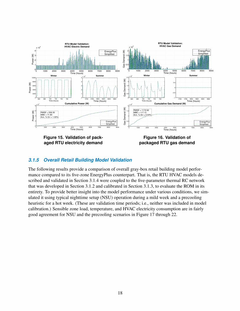
0 1000 2000 3000 4000 5000 6000 7000 8000 90000
1
2
3
4
x 104
Time (hours)
Po
we
r (W
)
RTU Model ValidationHVAC Electric Demand
EnergyPlusSimplified
660 680 700 720 740 7600
2000
4000
6000
8000
10000Winter
Time (hours)
Po
we
r (W
)
4760 4780 4800 4820 4840 48600
1
2
3
4
5x 10
4 Summer
Time (hours)
0 1000 2000 3000 4000 5000 6000 7000 8000 90000
2
4
6
8x 10
7 Cumulative Power (W)
Time (hours)
Po
we
r (W
)
RMSE = 55630MBE = 7180Ann Err = 100
EnergyPlusSimplified
0 1000 2000 3000 4000 5000 6000 7000 8000 90000
05
1
15
2
x 105
Time (hours)
Ga
s D
em
an
d (
W)
RTU Model ValidationHVAC Gas Demand
660 680 700 720 740 7600
05
1
15
2
25x 10
5 Winter
Time (hours)
Ga
s D
em
an
d (
W)
4760 4780 4800 4820 4840 48601
05
0
05
1Summer
Time (hours)
0 1000 2000 3000 4000 5000 6000 7000 8000 90000
05
1
15
2x 10
8 Cumulative Gas Demand (W)
Time (hours)
Ga
s D
em
an
d (
W)
RMSE = 117292MBE = 11713Ann Err = 054
EnergyPlusSimplified
EnergyPlusSimplified
Figure 15 Validation of pack- Figure 16 Validation of aged RTU electricity demand packaged RTU gas demand
315 Overall Retail Building Model Validation
The following results provide a comparison of overall gray-box retail building model perforshymance compared to its five-zone EnergyPlus counterpart That is the RTU HVAC models deshyscribed and validated in Section 314 were coupled to the five-parameter thermal RC network that was developed in Section 312 and calibrated in Section 313 to evaluate the ROM in its entirety To provide better insight into the model performance under various conditions we simshyulated it using typical nighttime setup (NSU) operation during a mild week and a precooling heuristic for a hot week (These are validation time periods ie neither was included in model calibration) Sensible zone load temperature and HVAC electricity consumption are in fairly good agreement for NSU and the precooling scenarios in Figure 17 through 22
18
5760 5780 5800 5820 5840 5860 5880 5900 5920 594080
70
60
50
40
30
20
10
0
10
20
Therm
al L
oad (
kW)
Retail Model ValidationZone Sensible Load NSU
EnergyPlus Simplified
5760 5780 5800 5820 5840 5860 5880 5900 5920 5940
3000
2000
1000
0
Cumulative Thermal Load (kW)
Time (hours)
Therm
al L
oad (
kW)
RMSE = 549MBE = 127Cum Err = 620
EnergyPlus
Simplified
5760 5780 5800 5820 5840 5860 5880 5900 5920 594018
20
22
24
26
28
30
Tem
pera
ture
(C)
Retail Model ValidationZone Temperature minus NSU
setpoint EnergyPlus Simplified
5760 5780 5800 5820 5840 5860 5880 5900 5920 5940
1000
2000
3000
4000
Cumulative Temperature (C)
Time (hours)Te
mpe
ratu
re (C
)
RMSE = 035MBE = 010Cum Err = 046
EnergyPlusSimplified
Figure 17 Retail sensible zone Figure 18 Retail zone mean air temshyload comparison for NSU scenario perature comparison for NSU scenario
4760 4780 4800 4820 4840 4860 4880 4900 4920 4940160
140
120
100
80
60
40
20
0
20
40
Th
erm
al L
oa
d (
kW)
Retail Model ValidationZone Sensible Load Precool
EnergyPlus Simplified
4760 4780 4800 4820 4840 4860 4880 4900 4920 4940
6000
4000
2000
0
Cumulative Thermal Load (kW)
Time (hours)
Th
erm
al L
oa
d (
kW)
RMSE = 588MBE = 211Cum Err = 566
EnergyPlus
Simplified
4760 4780 4800 4820 4840 4860 4880 4900 4920 494016
18
20
22
24
26
28
30
Tem
pera
ture
(C)
Retail Model ValidationZone Temperature minus Precool
setpoint EnergyPlus Simplified
4760 4780 4800 4820 4840 4860 4880 4900 4920 4940
1000
2000
3000
4000
Cumulative Temperature (C)
Time (hours)
Tem
pera
ture
(C)
RMSE = 024MBE = minus004Cum Err = minus019
EnergyPlusSimplified
Figure 19 Retail sensible zone load Figure 20 Retail zone mean air temperature comparison for precooling scenario comparison for precooling scenario
19
5760 5780 5800 5820 5840 5860 5880 5900 5920 59400
10
20
30
40
50
60
70
Energ
y (k
Wh)
Retail Model ValidationHVAC Electric Consumption NSU
EnergyPlus Simplified
5760 5780 5800 5820 5840 5860 5880 5900 5920 59400
1000
2000
3000
4000
Cumulative Energy (kWh)
Time (hours)
Energ
y (k
Wh)
RMSE = 494MBE = 074Cum Err = 347
EnergyPlusSimplified
4760 4780 4800 4820 4840 4860 4880 4900 4920 49400
20
40
60
80
100
120
Energ
y (k
Wh)
Retail Model ValidationHVAC Electric Consumption Precool
EnergyPlus Simplified
4760 4780 4800 4820 4840 4860 4880 4900 4920 49400
2000
4000
6000
Cumulative Energy (kWh)
Time (hours)
Energ
y (k
Wh)
RMSE = 649MBE = 004Cum Err = 011
EnergyPlusSimplified
Figure 21 Retail HVAC electricity con- Figure 22 Retail HVAC electricity consumpshysumption comparison for NSU scenario tion comparison for precooling scenario
32 Uncertainty Quantification
To illustrate the capabilities of the energy signal tool we adopted the five-parameter envelope (single-zone) ROM its parameters were identified from hourly surrogate training data derived from an EnergyPlus simulation of a five-zone retail building near the Chicago Midway Airport This model has five parameters for the building shell however 20 parameters are required for the building its use and HVAC systems each parameter is considered to be uncertain
321 Model Input Parameter Uncertainty
Input parameter distributions are characterized in this work using Gaussian distributions faults are modeled with triangular distributions although any other probability distribution may be selected In this work uncertainties are known varieties that are correctly quantified by an energy analyst using input distributions of choice faults are effects of unobserved uncertainties that affect the measured building performance but not the modeled predictions
The chosen distributions represent the best available knowledge of each uncertain model paramshyeter Input parameters are distributed around a mean that equals the nominal parameter value found from the parameter estimation process that has resulted in the validated ROM presented above A standard deviation of 10 of the mean is adopted for the uncertain input parameters
Adopting the five-parameter ROM 11 parameters are associated with the building shell and use and an additional nine parameters are associated with the HVAC system The seven nominal
20
building envelope parameters are shown in Table 3 the four use parameters are shown in Table 4 and the nine nominal HVAC-related model parameters are shown in Table 5
Table 4 Retail Building Use Parameters
Parameter Value Units
Lighting power density 3230 Wm2
Equipment power density 523 Wm2
Occupant density 71 m2per Infiltration flow rate 39 m3s
Table 5 Retail Building HVAC Parameters
Parameter Value Units
Supply fan efficiency 57 Maximum supply fan airflow 135 m3s Supply fan pressure rise 883 Pa DX coil rated capacity 319 kW DX coil rated sensible heat ratio 70 DX coil rated coefficient of performance (COP) 32 shyDX coil rated air mass flow rate 160 kgs Gas heating coil-rated capacity 457 kW Gas heating coil efficiency 80
To demonstrate the tool five of the 20 input parameters are considered uncertain lighting power density equipment power density occupant density DX coil-rated COP and gas heating coil efficiency The remaining 15 input parameters are taken at their nominal values In reality most of these 20 parameters would be uncertain at different levels of uncertainty
322 Operational and Equipment Faults
In spite of an energy analystrsquos best intentions and a belief that the model accurately reflects the building with all uncertainties undetected faults may affect building performance In this work a fault differs from a parameter uncertainty in that it is present without the knowledge of the energy analyst or building operator ie it is unobserved yet still affects the measured conditional distributions of building energy end use
We chose an additional six model parameters to represent such a faulted state Tehse are modeled by triangular distributions which may be asymmetrical The outdoor air fractionrsquos nominal value is 245 but may vary from 0 to 100 The airside economizer high limit temperature is nominally 28C but can vary between 12 and 40C Essentially at very low values of the
21
high limit temperature the economizer is disabled at high values the economizer operation is not overridden Heating and cooling temperature set points may differ from their assumed values with a random offset from -15 to +15 K Moreover the internal gains schedules may be expanded by up to 3 hours or contracted by up to 3 hours from the nominal building operation schedule Finally the schedules for internal gains from lighting and equipment may be shifted by up to 4 hours in each direction ie to earlier and later onsets Because the environment uses hourly time steps the schedule contractionexpansion and shift are rounded to the nearest full hour For the fault-free scenario the six fault parameters are kept at their nominal values For the faulted case all six fault parameters are randomly perturbed concurrently ie a very wide range of fault combinations is explored
Table 6 Fault Ranges
Parameter Nominal Minimum Maximum Units
Outdoor air fraction 245 0 100 Airside economizer high limit Cooling temperature set point Heating temperature set point Internal gains contractionexpansion Internal gains shift
28 228 217 10
800 am to 600 pm
12 -15 -15 -3 -4
40 +15 +15 + 3 + 4
C C C h h
Random sampling of 10000 annual samples for each case is presented here Because parameter combinations randomly drawn from the input distributions described above may lead to infeashysible model configurations for which no solution can be computed only valid model results are retained The sample rejection was put in place to deal with parameter combinations that cause simulation errors such as non-convergence and subsequent crashes Crashes are most often obshyserved when randomly sampling a wide range of HVAC equipment-rated parameters because the random sampling may not always produce physically consistent rated conditions Thus we expect that the wider the input parameter distributions the more frequently invalid model results are generated In the fault-free scenario 9994 of all samples were valid (six of 10000 failed) in the faulted scenario 9988 of all samples were valid (12 of 10000 failed)
The resultant conditional distribution of whole-building HVAC lighting (LTG) and plug elecshytricity EQP consumption is shown in Figure 23 Table 7 shows pertinent statistics of the same in units of [MWha] In the figure and table whole-building electricity (WBE) please define and add to nomenclature is the sum of HVAC LTG and miscellaneous electric loads EQP For fault-free and faulted cases the table shows the mean 10th 50th (median) and 90th percentiles along with the deterministic mean without consideration of any parameter uncertainty
It is evident that the uncertainty associated with the five selected parameters only slightly affects the mean but strongly affects the variance in the whole-building and submetered end uses The central 80 of the WBE consumption can be found within -7 and +8 from the determinisshytic mean in the fault-free case and within -24 and +20 from the deterministic mean in the
22
faulted case The influence of faults is stronger in the HVAC and LTG end uses compared to the EQP end use Given the dominance of HVAC and LTG end uses on whole-building consumption WBE faults strongly affect WBE as well Above all faults widen the energy distributions
100 200 300 400 500 600 7000
0005
001
0015
002
Prob
abilit
y
Whole Building Electric (MWh)50 100 150 200 250
0
002
004
006
008
Prob
abilit
y
HVAC Electric (MWh)
50 100 150 200 250 300 350 400 4500
0005
001
0015
002
Prob
abilit
y
Light Electric (MWh)10 20 30 40 50 60 70 80
0
002
004
006
008
01
Prob
abilit
y
Plug Electric (MWh)
FaultminusFreeFaulted
Figure 23 Distributions of whole-building HVAC lighting and plug electricity consumption
Table 7 Summary Statistics of Conditional Distributions of Whole-Building HVAC Lighting and Plug Electricity Consumption in [] in [MWha]
Percentile End-Use Case Mean 10th 50th 90th
WBE Deterministic 4163 Fault-free 100 93 100 108 Faulted 99 76 99 120
HVAC deterministic 1565 Fault-free 100 96 100 105 Faulted 96 79 97 112
LTG deterministic 2158 Fault-free 100 87 100 113 Faulted 100 71 99 130
EQP deterministic 441 Fault-free 100 87 100 113 Faulted 100 78 100 123
23
33 Decision Analysis
Comparing monitored data against a probable range of expected energy use is more insightful than comparing against a single number because it allows a building owner to assess the urgency of corrective actions that need to be taken If the measured energy use lies at the edge of the probable range of expected values given all the uncertainties in the model inputs the owner can be very confident that an issue requires attention In this work a decision-making tool was developed based on the probability distribution of model predictions to determine the expected utility of a range of available decisions suggesting the one that maximizes the expected utility The tool takes on the form of a modified traffic light with red yellow and green lights We adopted the perspective that a red light is shown both for high levels of overconsumption and high levels of underconsumption because a building consuming significantly less energy than expected may indicate an operational problem as significant as a building consuming too much A yellow signal is similarly used for cases of mild overconsumption and mild underconsumption A green light is reserved for measured building energy consumption that is in line with model expectations
As a first step a distribution of the model-predicted energy consumption (called Emod) was generated using Monte Carlo simulation as described in Section 32
Second the cases falling on the 5th median and 95th percentiles of the modeled energy distrishybutions were selected to represent low medium and high estimates of actual measured energy consumption (called Emeas) for fault-free and faulted scenarios The decision analysis compared the distribution of model-predicted energy consumption with Emeas to determine appropriate actions thus to illustrate the decision tool these three values of Emeas were taken from the samshypled distributions When physically implemented the measured energy consumption would be determined directly from building metering data
Third boundaries were computed from the measured energy consumption to define meaningful ranges of low and high levels of deviation in energy consumption Beginning with a low level of deviation let us define E0low such that it is Xlow percent below Emeas and E1low such that it is Xlow percent above Emeas
E0low = Emeas(1 minus Xlow)
E1low = Emeas(1 + Xlow)
Similarly for a high level of deviation letrsquos define E0high such that it is Xhigh percent below Emeas and E1high such that it is Xhigh percent above Emeas
E0high = Emeas(1 minus Xhigh)
E1high = Emeas(1 + Xhigh)
Of course Xlow lt Xhigh and we arbitrarily define Xlow to be 5 and Xhigh to be 10 ie a small deviation around the metered end use is plusmn5 and a large deviation plusmn10 It would be easy to adopt different values for Xlow and Xhigh for each building energy end use depending on its
24
temporal variability Once we have a conditional probability distribution of expected energy consumptions in hand we can make various kinds of statements Here we desire to report that the actual energy use is much higher somewhat higher similar somewhat lower or much lower than anticipated We further want to assign costs to making correct and incorrect statements and report the statement that has lowest expected cost
Fourth the empirical cumulative distribution of expected energy consumption was used to find the cumulative probabilities for the anticipated energy consumption to be below E0high (called P1) between E0high and E0low (called P2) between E0low and E1low (called P3) between E1low and E1high (called P4) and above E1high (called P5) Together these probabilities form the state probability vector PP = (P1P2P3P4P5)
T as shown in Figure 24
Figure 24 Relationship between deviation threshshyolds Xlow and Xhigh and state probability vector PP
Fifth we define a cost function K where cost is a function of state and action with a finite numshyber of states and a finite number of actions Therefore this cost function can be represented as a matrix Let us agree that there is one row per action and one column per state K(i j) ie cost of action i in state j Let action i = 1 display the lower red light (RL) on the modified traffic signal action i = 2 the lower yellow (YL) signal i = 3 a green (G) signal action i = 4 the upper yellow (YH) signal and finally i = 5 be displaying the upper red (RH) light Let j = 1 be the state that the model predicts a much lower (ML) energy consumption j = 2 a somewhat lower (SL) energy consumption j = 3 about the same (S) j = 4 a somewhat higher (SH) energy consumption and j = 5 a much higher (MH) energy consumption than the actual building Action vector Pa has thus five elements
25
Table 8 Decision Analysis State and Action
State j Anticipated Model Energy
Action i Much Lower Somewhat Lower Similar Somewhat Higher Much higher
Lower red Lower yellow Central green Upper yellow Upper red
K(RLML) K(YLML) K(GML)
K(YHML) K(RHML)
K(RLSL) K(YLSL) K(GSL)
K(YHSL) K(RHSL)
K(RLS) K(YLS) K(GS)
K(YHS) K(RHS)
K(RLSH) K(YLSH) K(GSH)
K(YHSH) K(RHSH)
K(RLMH) K(YLMH) K(GMH)
K(YHMH) K(RHMH)
An advantage of the presented decision analysis tool lies in its ability to individually set the costs of actions given certain states Here we make reasonable but somewhat arbitrary assumptions on the values of the cost matrix elements Showing an RL light when the model predicts ML energy consumption is assumed to have a cost of 4 (strong false negative lost savings opportunity) when the model predicts an SL energy consumption a cost of 3 (false negative) when the model predicts a similar energy consumption a cost of 2 (weak false negative) when the model predicts an SH energy consumption a cost of 1 (weak false negative) and finally when the model predicts MH energy consumption a cost of 0 (correct identification) Showing an RH light when the model predicts ML energy consumption is assumed to have a cost of 0 (correct identification) when the model predicts an SL energy consumption a cost of 1 (weak false positive) when the model predicts a similar energy consumption a cost of 2 (weak false positive) when the model predicts an SH energy consumption a cost of 3 (false positive) and finally when the model predicts MH energy consumption a cost of 4 (strong false positive unnecessary alarm) Similar arguments can be made for the remaining signals of a lower yellow (YL) a green and an upper yellow (YH) light and we yield the following cost matrix
⎡ K(RLML) K(RLSL) K(RLS) K(RLSH) K(RLMH)
⎤
K =
⎢⎢⎢⎢⎣
K(Y LML) K(GML)
K(Y HML) K(RHML)
K(Y LSL) K(GSL)
K(Y HSL) K(RHSL)
K(Y LS) K(GS)
K(Y HS) K(RHS)
K(Y LSH) K(GSH)
K(Y HSH) K(RHSH)
K(Y LMH) K(GMH)
K(Y HMH) K(RHMH)
⎥⎥⎥⎥⎦
⎡4 3 2 1 0
⎤
=
⎢⎢⎢⎢⎣
3 2 1 0
2 1 0 1
1 0 1 2
0 1 2 3
1 2 3 4
⎥⎥⎥⎥⎦ (37)
The expected cost vector for each action is found by multiplying the cost matrix K with the probability vector PP
E(Pa) = K middot PP
26
⎡ E (RL)
⎤ ⎡ K(RLML) K(RLSL) K(RLS) K(RL SH) K(RLMH)
⎤⎡P1⎤
E (Y L) K(Y LML) K(Y LSL) K(Y LS) K(Y LSH) K(Y LMH) P2⎢ ⎥ ⎢ ⎥⎢ ⎥⎢E (G)
⎥= ⎢
K(G ML) K(GSL) K(GS) K(GSH) K(GMH) ⎥⎢
P3⎥⎢ ⎥ ⎢ ⎥⎢ ⎥⎢
E (Y H)⎥ ⎢
K(Y HML) K(Y H SL) K(Y HS) K(Y HSH) K(Y HMH)⎥⎢
P4⎥⎣ ⎦ ⎣ ⎦⎣ ⎦
E (RH) K(RHML) K(RH SL) K(RHS) K(RHSH) K(RHMH) P5 ⎡ K(RLML)P1 + K(RLSL)P2 + K(RLS)P3 + K(RLSH)P4 + K(RLMH)P5
⎤
K(Y LML)P1 + K(Y LSL)P2 + K(Y LS)P3 + K(Y LSH)P4 + K(Y L MH)P5⎢ ⎥
= K(GML)P1 + K(GSL)P2 + K(GS)P3 + K(GSH)P4 + K(GMH)P5 (38)⎢⎢ ⎥⎥⎢
K(Y HML)P1 + K(Y HSL)P2 + K(Y H S)P3 + K(Y HSH)P4 + K(Y HMH)P5⎥⎣ ⎦
K(RHML)P1 + K(RHSL)P2 + K(RH S)P3 + K(RHSH)P4 + K(RHMH)P5
As suggested by utility theory the last step is to select the best action aopt in the face of uncershytainty ie activate that light which minimizes the expected cost
aopt = argminE(Pa)i
34 Bayesian Updating
Thus far the distributions of the uncertain model parameters were assumed to be Gaussian with a standard deviation equal to a fixed fraction of the parameter mean here 10 The choice of these distributions was made somewhat arbitrarily before any operational data was available from the actual building performance and termed before data because of its consideration prior to observation We believe that building performance measurements collected over an extended time period (ie after data) can be used to infer improved input parameter distributions by applying probability theory in general and Bayesrsquo theorem in particular See Jaynes (Jaynes 2003) for full development of Bayesian probability A brief explanation is provided below for information pertinent to this research
High-dimensional integrals associated with problems in computational physics lead to the develshyopment of Markov Chain Monte Carlo algorithms which can efficiently sample from probability distributions by exploiting the Markov property This has led to the explosion of Bayesian techshyniques with the Metropolis Algorithm as the breakthrough approach (named as one of the top 10 algorithms of the 20th century) (Cipra 2000) A probabilistic perspective not only provides insight into the relationship between sets of model parameters revealing tradeoffs and compenshysating interactions but also lends itself to a continuous model uncertainty quantification and tuning where the posterior distribution of an initial parameter estimate can be used as the prior for a subsequent parameter estimation update once new building performance data have been collected
Dodier used Bayesian (belief) networks for whole-building energy diagnostics (Dodier and Kreishyder 1999 Dodier et al 1998) Lauret et al (2006) demonstrated improvements over traditional parameter estimation methods by applying Bayesrsquo theorem to determine better estimates of conshyvection coefficients for a radiant barrier roof system model More recently Booth et al (2012)
27
used London housing stock models for hierarchical modeling with considerations of internal heating set points fraction of space heating air leakage heating system COP window U-value and window-to-wall ratio
In this work the Bayesian inference of uncertain model parameters relies on the extension of a previously developed technique (Neumann et al 2011) It has benefits over traditional methods because prior knowledge of the system can be directly incorporated into the estimation task and methods for addressing sensor noise are inherent to the Bayesian approach The inference can essentially be thought of as fitting a joint probability distribution to a measured dataset Specifishycally conditional probabilities are related through the product rule to derive Bayesrsquo theorem and allow consideration of before data and after data states of knowledge The prior probability distribution is updated with any measured data to form the posterior probability distribution which represents the state of knowledge in any inference task We propose a periodic process where model input parameter distributions are updated daily weekly monthly or for a similar period of interest As new measurements become available data effectively shape the distribution of expected building energy use according to the information gleaned from a combination of prior knowledge and sensor data uncertainty is still present but should decrease with additional data and understanding of the relationships among variables
The probability of parameter set Θ given measured data D and knowledge of the system K can be written as posterior probability p(Θ|DK) Bayesrsquo theorem then allows the conditional probability p(Θ|DK) to be computed from p(Θ|K) p(D|ΘK) and p(D|K) as shown in Equation 39
p(D|ΘK)p(Θ|DK) = p(Θ|K) (39)
p(D|K)
where p(Θ|K) represents prior knowledge about parameter values p(D|ΘK) represents the likeshylihood of observing the measured dataset D given a particular parameter set Θ and knowledge of the system K and p(D|K) is the probability of observing the dataset Ignoring the reference to system knowledge K the relation can be written in alternate form where the numerator reshymains the product of likelihood and prior and the denominator is a normalization factor so that posterior probabilities sum to unity
p(Θ)p(D|Θ)p(Θ|D) = (310)
sum p(Θi)p(D|Θi) i
Assuming random Gaussian noise about a measured datum Di the likelihood of an observation can be determined from its location within the normal distribution with standard deviation σε this is not in nomenclature centered at micro equal to the measured datum
p(Di|Θ) = radic 1
exp(minus(Di minus Mi)
2 ) (311)
σε 2π 2σε2
where Mi is the model output given the parameter set Θ
28
Further assuming independent errors the likelihood is that the entire dataset is simply the prodshyuct of the likelihoods of all individual points The assumption is likely valid for common HVAC sensors (eg temperature probes) but correlated errors could be handled with a slightly different formulation that is indicative of a fault model Measurement errors are often correlated because of for example hysteresis error or linearity error If such correlated errors are of concern a Bayesian (or other probabilistic) method may be used that can accommodate correlated measureshyments This work nonetheless assumes uncorrelated energy consumption measurements thus it ignores autocorrelation of errors which is estimated to be small For the dynamics and time range considered in this problem model structure is considered more important with respect to data fit than noise correlation From this model assumption we derive the easily computable likelihood function given by Equation 312
The likelihood function is maximized when the exponential term is minimized which occurs as the modeled data approach the measured (or surrogate) data When uniform priors are used with Equation 312 in a Bayesian calibration context the most likely parameters are equivalent to those that would be found using a least squares approach because the exponential term in Equation 312 is essentially the sum of squared errors (Pavlak et al 2014)
minus1 n
1 2p(D|Θ) = radic n exp sum (Di minus Mi) (312)
2σ2-σε 2π ε i=1
Evaluating Equation 312 directly can pose numerical issues because a small range of σε values results in a large range of likelihoods Double precision computing environments are typically capable of evaluating floating point numbers on the order of 10minus308 to 10308 This means that when using 3 weeks of hourly data (ie n = 504) σε must approximately be in the range of [0115] Values outside this range will cause the likelihood (and consequently the posterior) to evaluate to Inf NaN or 0 regardless of the time series fit These numerical issues can be alleviated by computing the natural logarithm of the posterior rather than the posterior directly (Lauret et al 2006 Sivia and Skilling 2006)
To compute the natural log of the posterior first the log of both sides of Equation 310 is taken ⎛ ⎞
p(Θ)p(D|Θ)ln(p(Θ|D)) = ln (313)⎝
sum p(Θi)p(D|Θi)⎠
i
The right-hand side of Equation 313 can be separated using logarithm product and quotient rules
ln(p(Θ|D)) = ln(p(Θ)) + ln(p(D|Θ)) minus ln sum p(Θi)p(D|Θi) (314)
i
29
The log-likelihood term of Equation 314
n1 minus1 2ln(p(D|Θ)) = ln radic n exp sum (Di minus Mi) (315) -σε 2π 2σε
2i=1
can be further simplified by applying product and quotient rules as shown in Equations 316 and 317 respectively
n1 minus1 2ln (p(D|Θ)) = ln radic n + ln exp sum (Di minus Mi) (316) -σε 2π 2σε
2i=1
radic nminus1 2ln(p(D|Θ)) = ln(1) minus ln ((
σε 2π
)n)+ ln exp sum (Di minus Mi) (317)
2σ2ε i=1
With ln(1) = 0 and the power rule can be applied to the middle term of the right-hand side The last term of the right-hand side simplifies because of to logarithmic identity to produce Equation 318
radic nminus1ln(p(D|Θ)) = minusn ln
(σε 2π
)+ sum (Di minus Mi)
2 (318)2σ2
ε i=1
Recombining the simplified log-likelihood of Equation 318 with the log-posterior equation of Equation 314 yields
radic n1 2ln(p(Θ|D)) = ln(p(Θ)) minus n ln(
σε 2π
)minus sum (Di minus Mi) (319)
2σ2ε i=1
minus ln sum p(Θi)p(D|Θi) i
The last term of the right-hand side of Equation 319 is ultimately a constant number subtracted from each individual ln(p(Θi)p(D|Θi)) value Because the value of this constant term does not impact the shape or relative information of the posterior it could be thought of as an arbitrary constant C
radic n1 2ln(p(Θ|D)) = ln(p(Θ)) minus n ln(
σε 2π
)minus sum (Di minus Mi) +C (320)
2σ2ε i=1
The constant term can be moved to the left-hand side of the equation producing Equation 321
radic n1 2ln(p(Θ|D)) minusC = ln(p(Θ)) minus n ln(
σε 2π
)minus sum (Di minus Mi) (321)
2σ2ε i=1
30
Because the objective is to avoid numerical underflow or overflow prescribing
C = max radic
ln(p(Θ)) minus n ln(
σε 2π
) minus
1 n
sum 2(Di minus Mi) (322)2σε
2i=1
shifts all points so that the maximum is 0 A maximum value of 0 in the ln space ensures that all values will be mapped to the interval [01] when taking the exponential After taking exponenshytials the values can be scaled by a constant so that probabilities sum to unity
The σε value is a noise term with physical interpretation Here there are three energy signals of interest HVAC lighting and equipmentndashall electrical terms with the error associated with minor fluctuations not incorporated in the physical model As previously stated prescribing an appropriate σε is necessary to prevent underflow or overflow which causes the inference task to crash from numerical issues The most appropriate σε value can be found by maximum a posteriori (MAP) estimation MAP is used to obtain a point estimate of σε by placing a prior distribution over σε and finding the maximum posterior mode according to the empirical data Because the HVAC lighting and equipment energy signals are considered independent in this study the MAP estimate of σε HVAC σε LT G and σε EQP were performed separately with a uniform prior on each σε set between 0 and 15 of the magnitude of the full individual signals
With the appropriate and optimal σε set for each signal it was then possible to calculate the probability of observing various energy signals as a function of the uncertainty parameters Because the signals are considered independent the joint probability of the building state is a product of the individual probabilities
p =prodpi = pHVAC pLT G pEQP (323) i
With the joint posterior probability distribution available from the equation above it was then possible to sample from the posterior directly or marginalize over all parameters not of interest and form a new prior That is the updating process is prior rarr posterior rarr prior The optimal updating period is a function of the building energy dynamics and available data
31
4 Results
Results are presented that (1) exemplify the decision support aspect of the tool and (2) illustrate the updating of the uncertain model parameters based on measured data
41 Decision Support Case Studies
The decision analysis results presented here are separated into fault-free and faulted scenarios In the fault-free scenario the high medium and low consumption values (surrogates of measured building energy consumption) are drawn from the conditional energy consumption distributions without faults and the decision analysis is based on the same distribution In contrast in the faulted scenario the high medium and low consumption values are drawn from the conditional energy consumption distributions including faults and the decision analysis is based on the distribution excluding faults
The results are shown as a matrix of figures The first row shows the whole-building electricity WBE consumption results for the last year then last month then last week followed by the last day The second row shows the HVAC energy consumption results for the time periods the third row shows the lighting LTG results and lastly the fourth row shows the EQP results Each of the 16 figure panels reveals a box plot1 Larger and smaller values respectively are shown as outliers of the expected energy consumption value for the time period of interest a diamond marker superimposed on the box plot to indicate the surrogate actual consumption value Emeas and on the left margin the energy signal tool with the signal chosen for the resultant cumulative probabilities PP cost matrix C and deviation thresholds Xlow and Xhigh The central green light separates cases of mild (YH) and strong (RH) overconsumption above the green light from the cases of of mild (YL) and strong (RL) underconsumption below the green light The particular traffic signal-inspired design is one of many possible designs chosen for illustration here thus many other valid designs can be conceived Moreover the planned field implementation of this energy signal tool would likely not show the box plots but only the signals Finally if only whole-building energy WBE measurements are available the tool would reveal only the top row of WBE versus the four time periods In contrast when submetering of HVAC LTG and EQP is available the lower three rows would be shown and the top WBE row omitted because it would not offer additional insight
1Box plots shown in this report adopt the common notation that the box occupies the interquartile range (IQR) from the lower (25th percentile) to the upper (75th percentile) The whiskers extend to the minimum and maximum values if these are less than 15 times the IQR below the lower or 15 times the IQR above the upper quartile
32
411 Fault-Free Scenario
4111 High Energy Consumption Case
Beginning on August 30 with the high energy consumption case at the 95th percentile a mild overconsumption is shown for all time scales for WBE and HVAC LTG and EQP show strong overconsumption for all time scales
350
400
450
500
WBEYear
MWh
35
40
45
50
55
WBEMonth
MWh
8
9
10
11
12
WBEWeek
MWh
1100
1200
1300
1400
1500
1600
1700
WBEDay
kWh
140
150
160
170
180
HVACYear
MWh
18
20
22
24
26
28
HVACMonth
MWh
4
45
5
55
6
HVACWeek
MWh
500
550
600
650
700
750
HVACDay
kWh
150
200
250
300
LTGYear
MWh
12
14
16
18
20
22
24
LTGMonth
MWh
3
35
4
45
5
55
LTGWeek
MWh
500
600
700
800
900
LTGDay
kWh
30
35
40
45
50
55
60
EQPYear
MWh
25
3
35
4
45
5
EQPMonth
MWh
06
07
08
09
1
11
EQPWeek
MWh
80
100
120
140
160
EQPDay
kWh
Figure 25 Fault-free high consumption case beginning August 30 (meashysured consumption data are indicated by diamonds in each figure)
4112 Medium Energy Consumption Case
The medium consumption cases for August and February show consistency between WBE HVAC and LTG green lights are shown for all time scales and the EQP consumption is low Because the EQP contribution to the total is small the WBE signal is not swayed to show a low yellow light
33
350
400
450
500
WBEYear
MWh
35
40
45
50
55
WBEMonth
MWh
8
9
10
11
12
WBEWeek
MWh
1100
1200
1300
1400
1500
1600
1700
WBEDay
kWh
140
150
160
170
180
HVACYear
MWh
18
20
22
24
26
28
HVACMonth
MWh
4
45
5
55
6
HVACWeek
MWh
500
550
600
650
700
750
HVACDay
kWh
150
200
250
300
LTGYear
MWh
12
14
16
18
20
22
24
LTGMonth
MWh
3
35
4
45
5
55
LTGWeek
MWh
500
600
700
800
900
LTGDay
kWh
30
35
40
45
50
55
60
EQPYear
MWh
25
3
35
4
45
5
EQPMonth
MWh
06
07
08
09
1
11
EQPWeek
MWh
80
100
120
140
160
EQPDay
kWh
Figure 26 Fault-free medium consumption case beginning August 30 (measured consumption data are indicated by diamonds in each figure)
4113 Low Energy Consumption Case
In the low consumption case it is interesting to note that the WBE signal shows a strong unshyderconsumption (low red) driven by the corresponding LTG signal even though HVAC conshysumption is similar to the model expectation (green) and EQP is only a mild underconsumption This case reveals the importance of submetering Without it it would not have been possible to isolate that LTG causes the warning HVAC could be ignored and EQP could be given less consideration
34
350
400
450
500
WBEYear
MWh
35
40
45
50
55
WBEMonth
MWh
8
9
10
11
12
WBEWeek
MWh
1100
1200
1300
1400
1500
1600
1700
WBEDay
kWh
140
150
160
170
180
HVACYear
MWh
18
20
22
24
26
28
HVACMonth
MWh
4
45
5
55
6
HVACWeek
MWh
500
550
600
650
700
750
HVACDay
kWh
150
200
250
300
LTGYear
MWh
12
14
16
18
20
22
24
LTGMonth
MWh
3
35
4
45
5
55
LTGWeek
MWh
500
600
700
800
900
LTGDay
kWh
30
35
40
45
50
55
60
EQPYear
MWh
25
3
35
4
45
5
EQPMonth
MWh
06
07
08
09
1
11
EQPWeek
MWh
80
100
120
140
160
EQPDay
kWh
Figure 27 Fault-free low consumption case beginning August 30 (meashysured consumption data are indicated by diamonds in each figure)
412 Faulted Scenarios
In the faulted scenarios the three cases are drawn from much wider distributions as shown in Figure 23
4121 High Energy Consumption Case
The high consumption case for August 30 shows consistency between WBE HVAC and LTG RH lights are shown for all time scales and the EQP consumption is close to model expectation However because the EQP contribution to the total is small the WBE signal is not swayed to show a low green light
35
350
400
450
500
WBEYear
MWh
35
40
45
50
55
WBEMonth
MWh
8
9
10
11
12
WBEWeek
MWh
1100
1200
1300
1400
1500
1600
1700
WBEDay
kWh
140
150
160
170
180
HVACYear
MWh
18
20
22
24
26
28
HVACMonth
MWh
4
45
5
55
6
HVACWeek
MWh
500
550
600
650
700
750
HVACDay
kWh
150
200
250
300
LTGYear
MWh
12
14
16
18
20
22
24
LTGMonth
MWh
3
35
4
45
5
55
LTGWeek
MWh
500
600
700
800
900
LTGDay
kWh
30
35
40
45
50
55
60
EQPYear
MWh
25
3
35
4
45
5
EQPMonth
MWh
06
07
08
09
1
11
EQPWeek
MWh
80
100
120
140
160
EQPDay
kWh
Figure 28 Faulted high consumption case beginning August 30 (meashysured consumption data are indicated by diamonds in each figure)
4122 Medium Energy Consumption Case
On an annual basis the medium consumption case leads to the expected green lights On time scales of months and shorter we can observe HVAC mild and strong underconsumption
36
350
400
450
500
WBEYear
MWh
35
40
45
50
55
WBEMonth
MWh
8
9
10
11
12
WBEWeek
MWh
1100
1200
1300
1400
1500
1600
1700
WBEDay
kWh
140
150
160
170
180
HVACYear
MWh
18
20
22
24
26
28
HVACMonth
MWh
4
45
5
55
6
HVACWeek
MWh
500
550
600
650
700
750
HVACDay
kWh
150
200
250
300
LTGYear
MWh
12
14
16
18
20
22
24
LTGMonth
MWh
3
35
4
45
5
55
LTGWeek
MWh
500
600
700
800
900
LTGDay
kWh
30
35
40
45
50
55
60
EQPYear
MWh
25
3
35
4
45
5
EQPMonth
MWh
06
07
08
09
1
11
EQPWeek
MWh
80
100
120
140
160
EQPDay
kWh
Figure 29 Faulted medium consumption case beginning August 30 (measured consumption data are indicated by diamonds in each figure)
4123 Low Energy Consumption Case
The low consumption case at the 5th percentile of the faulted distribution shows a consistent RL light for all end uses and time scales independent of season
37
300
350
400
450
500
WBEYear
MWh
35
40
45
50
55
WBEMonth
MWh
7
8
9
10
11
12
WBEWeek
MWh
1000
1100
1200
1300
1400
1500
1600
1700
WBEDay
kWh
130
140
150
160
170
180
HVACYear
MWh
18
20
22
24
26
28
HVACMonth
MWh
4
45
5
55
6
HVACWeek
MWh
500
550
600
650
700
750
HVACDay
kWh
150
200
250
300
LTGYear
MWh
12
14
16
18
20
22
24
LTGMonth
MWh
3
35
4
45
5
55
LTGWeek
MWh
500
600
700
800
900
LTGDay
kWh
30
35
40
45
50
55
60
EQPYear
MWh
25
3
35
4
45
5
EQPMonth
MWh
06
07
08
09
1
11
EQPWeek
MWh
80
100
120
140
160
EQPDay
kWh
Figure 30 Faulted low consumption case beginning August 30 (meashysured consumption data are indicated by diamonds in each figure)
Finally we present a sample illustration of how such a decision analysis tool would be deployed in the management of distributed commercial buildings Imagine a building operator is responsishyble for the energy-efficient operation of four buildings in a city Building 1 appears to be healthy all end uses show green signals for all four time scales building 2 suffers from overconsumption problems in the HVAC system that manifest themselves in the last day week and month buildshying 3 exhibits underconsumption in LTG especially during the last week which could speak to failed light sources or delamping measures not yet accounted for in the model finally building 4 suffers from multiple symptoms overconsumption in HVAC and EQP and underconsumption in LTG
38
Figure 31 Example of four buildings managed by a building operator
42 Bayesian Parameter Updating Case Studies
Results related to the probabilistic inference and updating of the uncertain model parameters are presented for September 21 at which point measurements over the past 30 days are used to update the five input parameter distributions that are deemed uncertain The high consumption case representing the 95th percentile of the fault-free conditional distributions is used to compute the likelihood functions for HVAC LTG and EQP for each of the nearly 10000 parameter
39
combinations Based on the simplifying assumptions articulated above we can then find the marginal posterior distribution for each selected uncertain parameter Please note that white Gaussian noise with a signal-to-noise ratio of 25 was added to the time series data of the high consumption case to simulate common measurement noise affecting building measurements Recent work by the same authors has shown the Bayesian inference approach to be robust with respect to a wide range of signal-to-noise ratios and noise colors (Pavlak et al 2014)
Table 9 shows the nominal values used to generate the prior input parameter distributions as well as the parameter values associated with the low medium and high cases investigated in this section The latter represent the ground truth values that will be compared to the posterior distributions for each model parameter to determine whether the measured data are used to update our belief of the uncertain parameters in a way that is consistent with the ground truth data
The table shows that several individual parameters appear inconsistent with the case they beshylong to As one example in the low consumption case the DX coil-rated COP is 31 which is below the nominal value One would expect a higher COP to be associated with the low conshysumption case However given the tradeoffs between lighting and equipment power consumption and the efficiency of the cooling equipment the low consumption case at the 5th percentile of 10000 simulation runs was the result of a less efficient RTU with strongly reduced lighting and equipment power densities The median consumption case resulted from a slightly higher lighting power density lower equipment power density lower occupant density and higher RTU COP all relative to the nominal values The high consumption case at the 95th percentile of all cases is characterized by higher lighting equipment and occupancy densities and lower HVAC equipment efficiency In this case of higher consumption the individual parameter values are all consistent with the theme of the case
Later sections discuss that whatever tradeoffs were at play in leading to the low medium and high cases the Bayesian parameter updating process is changing the posterior parameter disshytributions toward the ground truth values that form the basis of the measured (here surrogate) consumption data To that effect each of the following figures 32 to 46 shows the sampled prior distribution of the uncertain parameter as blue bars the sampled posterior distribution as red bars and the ground truth value that formed the basis of the surrogate measured data as a green vertical line
Gas heating efficiency should have no impact on electricity consumption thus increased electricshyity consumption should be independent from gas heating coil efficiency All the figures showing gas heating efficiency distributions illustrate that the gas heating efficiency posterior distribution is being smeared out ie becoming less informative because the evidence used in the likelihood function does not offer any clear clues about how to shape the posterior Although we show the prior and posterior distributions for gas heating efficiency for all three cases the independence of electricity consumption from gas heating efficiency is seen in a widening posterior in each case
40
Table 9 Building Model Truth Parameters
Parameter Nominal Low Medium High Units
Lighting power density 3230 2699 3309 3615 Wm2
Equipment power density 523 492 496 594 Wm2
Occupant density 0141 0149 0137 0151 perm2
DX coil rated COP 320 310 339 294 -Gas heating coil efficiency 80 74 70 77
421 High Energy Consumption Case
Figures 32 through 36 clearly illustrate how the measured data would be harnessed to update our belief about the uncertain parameters Each figure shows the empirical prior distribution as blue bars the empirical posterior distribution is shown as red bars Where the two distributions overlap a darker purple hue appears As stated above in the high energy consumption case all individual building parameter truth values are consistent with the theme of high energy conshysumption Lighting and equipment power density posteriors move to higher values relative to the nominal values that served as the mean of the normal prior distributions and gravitate toward the truth values (green vertical lines) used to generate the surrogate measured data Similarly occupancy densities in people per square meter are also slightly higher and the DX coil-rated COP is significantly lower than the nominal value gravitating toward the truth values Thus the Bayesian inference learns the truth values that form the basis of the measured data
Figure 32 Lighting power density prior (blue) and posterior (red) distributions on
September 21 based on past 30 days of high energy consumption Truth
value is shown as a green vertical line
Figure 33 Equipment power density prior (blue) and posterior (red) distribushytions on September 21 based on past 30 days of high energy consumption Truth value is shown as a green vertical line
41
Figure 34 Occupant density prior (blue) and posterior (red) distributions on
September 21 based on past 30 days of high energy consumption Truth
value is shown as a green vertical line
Figure 35 DX Coil Rated COP prior (blue) and posterior (red) distributions on
September 21 based on past 30 days of high energy consumption Truth
value is shown as a green vertical line
Figure 36 Gas heating coil efficiency prior (blue) and posterior (red) distributions on September 21 based on past 30 days of high energy consumption Truth value is shown as a green vertical line
422 Medium Energy Consumption Case
Figures 37 through 41 show how in the medium consumption case the data reveal the tradeoffs that form the basis of the medium consumption case A slightly higher lighting power density is compensated for by a significantly lower equipment power density because these two have the identical effects of adding convective internal gains to the sensible energy balance paired with slightly higher COPs Occupant density distribution has not materially changed from prior
42
to posterior in the medium consumption case As in the high consumption case the posterior distributions (except for gas heating efficiency as explained above) have moved in the direction of the truth values that form the foundation of the surrogate measured data
Figure 37 Lighting power density prior (blue) and posterior (red) distributions
on September 21 based on past 30 days of medium energy consumption Truth value is shown as a green vertical line
Figure 38 Equipment power density prior (blue) and posterior (red) distributions
on September 21 based on past 30 days of medium energy consumption Truth value is shown as a green vertical line
Figure 39 Occupant density prior (blue) and posterior (red) distributions on
September 21 based on past 30 days of medium energy consumption Truth value is shown as a green vertical line
Figure 40 DX Coil Rated COP prior (blue) and posterior (red) distributions on
September 21 based on past 30 days of medium energy consumption Truth value is shown as a green vertical line
43
Figure 41 Gas heating coil efficiency prior (blue) and posterior (red) distributions on September 21 based on past 30 days of medium
energy consumption Truth value is shown as a green vertical line
423 Low Energy Consumption Case
Figures 42 through 46 again clearly illustrate how the measured data would be harnessed to update our belief about the uncertain parameters In the low consumption case the data suggest significantly lower lighting and equipment power densities although occupant density seems to materially impact the measured data which lead to a virtually unchanged posterior
As shown in Table 9 the truth value of the DX coil-rated COP is slightly lower than the nominal value which is opposite to the theme of lower energy consumption As explained above the slightly inferior COP is more than compensated for by significantly lower lighting and equipment power densities The posterior COP distribution is close2 to the prior but slightly less than it feels like something is missing here suggesting that the Bayesian inference has learned the truth value
As before electricity consumption should not and does not have informative power for gas heating efficiency leaving the posterior smeared out relative to the prior
2A very heuristic visual interpretation of close was used We simply encourage the reader to determine in which direction the posterior distribution mass has been moving to the left to the right or virtually unchanged relative to the prior distribution In particular the point of using such loose language is to avoid comparing the empirical prior and posterior distributions with a more rigorous metric such as the maximum distance of the two cumulative distribution functions as used in the two-sample Kolmogorov-Smirnof test Future work will look into more rigorous metrics to automate the update process The point we wanted to make in this work however is that evidence is collected and used to inform updates of the input parameter distributions
44
Figure 42 Lighting power density prior (blue) and posterior (red) distributions
on September 21 based on past 30 days of low energy consumption Truth value is shown as a green vertical line
Figure 44 Occupant density prior (blue) and posterior (red) distributions on
September 21 based on past 30 days of low energy consumption Truth
value is shown as a green vertical line
Figure 43 Equipment power density prior (blue) and posterior (red) distribushytions on September 21 based on past 30 days of low energy consumption Truth value is shown as a green vertical line
Figure 45 DX Coil Rated COP prior (blue) and posterior (red) distributions
on September 21 based on past 30 days of low energy consumption Truth value is shown as a green vertical line
45
Figure 46 Gas heating coil efficiency prior (blue) and posterior (red) distributions on September 21 based on past 30 days of low
energy consumption Truth value is shown as a green vertical line
46
5 Summary and Conclusions
A prototype energy signal tool was demonstrated for operational whole-building and system-level energy performance assessment The purpose of the tool is to give an assessment that a building operator or other user can quickly comprehend Toward this end the energy signal tool estimates energy use for various end uses from a low-order lumped-parameter model taking into account uncertainty (via a Monte Carlo method) in model parameters and inputs The result of the modelshying phase is a probability distribution over estimated energy use The range of estimated energy use is divided into intervals based on the observed energy use and the probability that energy use is in an interval is computed as the mass of the estimated energy use distribution in that interval An indicator (traffic light color) is chosen to minimize misclassification cost Model parameter distributions are adjusted over time via Bayesian updating
The experimental study investigated whole-building energy signal accuracy in the presence of uncertainty and faults at the submetered level which may lead to tradeoffs at the whole-building level that are not detectable without submetering Submetering of end uses is recommended to avoid confounding underconsumption and overconsumption among various end uses An examshyple of four building energy signal displays is offered to illustrate energy performance features that could be detected by the energy signal tool The Bayesian inference results presented show that observations can be used to periodically update model parameter distributions and that the posterior distributions indeed gravitate toward the ground truth parameter values that formed the basis of the surrogate measured data We presented results for a 30-day learning cycle
Future improvements in the inference process would eliminate the assumptions of temporal independence of subsequent observations of a particular variable and structural independence of multiple observed variables Accounting for covariance among observed variables will help to better attribute observations to individual model parameters
47
Bibliography
Attia S Gratia E Herde AD Hensen JL (2012) ldquoSimulation-based decision support tool for early stages of zero-energy building designrdquo Energy and Buildings 49(0) pp 2 ndash 15
Augenbroe G Castro D Ramkrishnan K (2009) ldquoDecision model for energy performance improvements in existing buildingsrdquo Journal of Engineering Design and Technology 7(1) pp 21 ndash 36
Balcomb J Curtner A (2000) ldquoMulti-criteria decision-making process for buildingsrdquo Energy Conversion Engineering Conference and Exhibit Vol 1 pp 528 ndash 535 Las Vegas NV USA IEEE
Basso N Garavaglia E Sgambi L Imagawa N (2013) Natural hazards vs Decision-making processes in buildings life cycle management New York NY USA CRC Press
Bauermann K Spiecker S Weber C (3 2014) ldquoIndividual decisions and system development Integrating modelling approaches for the heating marketrdquo Applied Energy 116 pp 149ndash158
Booth A Choudhary R Spiegelhalter D (Feb 2012) ldquoHandling uncertainty in housing stock modelsrdquo Building and Environment 48(0) pp 35ndash47
Bracken C Rajagopalan B Prairie J (Mar 2010) ldquoA multisite seasonal ensemble streamflow forecasting techniquerdquo Water Resources Research 46(3) pp 1ndash12 URL httpdoiwileycom1010292009WR007965
Brandemuehl M Shauna G Inger A (1993) ldquoHVAC2 Toolkit Algorithms and Subroutines for Secondary HVAC System Energy Calculationsrdquo ASHRAE Atlanta GA
Braun JE Chaturvedi N (2002) ldquoAn inverse gray-box model for transient building load predictionrdquo HVACampR Research 8(1) pp 73ndash100
Burkhart MC Heo Y Zavala VM (2014) ldquoMeasurement and verification of building systems under uncertain data A Gaussian process modeling approachrdquo Energy and Buildings 75 pp 189 ndash 198
Chaturvedi N Braun J Bernhard R (2000) Analytical Tools for Dynamic Building Conshytrol Implementation of Thermal Storage in Building Mass American Society of Heating Refrigerating and Air-Conditioning Engineers
Choi JH Aziz A Loftness V (2009) ldquoDecision support for improving occupant environmenshytal satisfaction in office buildings The relationship between sub-set of IEQ satisfaction and overall environmental satisfactionrdquo Ninth International Conference of Healthy Buildings p 747 Syracuse NY USA
48
Cipra BA (2000) ldquoThe best of the 20th century Editors name top 10 algorithmsrdquo SIAM news 33(4) pp 1ndash2
Crawley DB Lawrie LK Winkelmann FC Buhl WF Huang YJ Pedersen CO Strand RK Liesen RJ Fisher DE Witte MJ et al (2001) ldquoEnergyPlus creating a new-generation building energy simulation programrdquo Energy and Buildings 33(4) pp 319ndash331
Das S Chew M Poh KL (2010) ldquoMulti-criteria decision analysis in building maintainability using analytical hierarchy processrdquo Construction Management and Economics 28(10) pp 1043 ndash 1056
De Farias C Soares H Pirmez L Delicato F Santos I Carmo LF De Souza J Zomaya A Dohler M (2014) ldquoA control and decision system for smart buildings using wireless sensor and actuator networksrdquo European Transactions on Telecommunications 25(1) pp 120 ndash 135
De Wit S Augenbroe G (2002) ldquoAnalysis of uncertainty in building design evaluations and its implicationsrdquo Energy and Buildings 34(9) pp 951 ndash 958
Deru M Field K Studer D Benne K Griffith B Torcellini P Halverson M Winiarski D Liu B Rosenberg M Huang J Yazdanian M Crawley D (2010) US Department of Energy Commercial Reference Building Models of the National Building Stock Washington DC US Department of Energy Energy Efficiency and Renewable Energy Office of Building Technologies
Diakaki C Grigoroudis E Kabelis N Kolokotsa D Kalaitzakis K Stavrakakis G (2010) ldquoA multi-objective decision model for the improvement of energy efficiency in buildingsrdquo Energy 35(12) pp 5483 ndash 5496
Diakaki C Grigoroudis E Kolokotsa D (2013) ldquoPerformance study of a multi-objective mathematical programming modelling approach for energy decision-making in buildingsrdquo Energy 59 pp 534 ndash 542
Dodier R Kreider J (1999) ldquoWhole Building Energy Diagnosticsrdquo ASHRAE Trans 105(1) pp 579ndash589
Dodier RH Curtiss PS Kreider JF (1998) ldquoSmall-scale on-line diagnostics for an HVAC systemrdquo Transactions-American Society Of Heating Refrigerating And Air Conditioning Engineers 104 pp 530ndash539
DOE U (2010) ldquoEnergyPlus Engineering Referencerdquo The Reference to EnergyPlus Calculashytions URL httpapps1eereenergygovbuildingsenergypluspdfs engineeringreferencepdf
49
Filippoupolitis A Gelenbe E (2009) ldquoA decision support system for disaster management in buildingsrdquo Summer Computer Simulation Conference pp 141 ndash 147 Society for Modeling amp Simulation International
Florita AR Brackney LJ Otanicar TP Robertson J (2013) ldquoClassification of Commercial Building Electrical Demand Profiles for Energy Storage Applicationsrdquo Journal of Solar Energy Engineering 135(3) p 031020
Gulbinas R Jain RK Taylor JE (2014) ldquoBizWatts A modular socio-technical energy management system for empowering commercial building occupants to conserve energyrdquo Applied Energy In-Press
Gultekin P Anumba CJ Leicht RM (2013) ldquoTowards an integrated process model and decision support system for high performance green retrofitsrdquo Architectural Engineering Conference 2013 pp 912 ndash 923 State College PA United states
Heo Y Augenbroe G Choudhary R (2011) ldquoRisk analysis of energy-efficiency projects based on bayesian calibration of building energy modelsrdquo Twelth Conference of International Building Performance Simulation Association pp 2579 ndash 2586 Sydney AUS
Heo Y Zavala VM (2012) ldquoGaussian process modeling for measurement and verification of building energy savingsrdquo Energy and Buildings 53 pp 7 ndash 18
ISO E (2007) ldquo13790 2007rdquo Energy performance of buildings-Calculation of energy use for space heating and cooling
Jaynes ET (2003) Probability theory the logic of science Cambridge university press
Judkoff R Balcomb J Hancock C Barker G Subbarao K (2000) Side-By-Side Thermal Tests of Modular Offices A Validation Study of the STEM Method NREL Report TP-550shy23940 National Renewable Energy Laboratory
Judkoff R Wortman D OrsquoDoherty B Burch J (20081983) Methodology for Validating Building Energy Analysis Simulations NREL Report No TP-550-42059 National Renewable Energy Laboratory Golden CO
Kiluk S (11 2014) ldquoDynamic classification system in large-scale supervision of energy effishyciency in buildingsrdquo Applied Energy 132 pp 1ndash14
Kolokotsa D Diakaki C Grigoroudis E Stavrakakis G Kalaitzakis K (2009) ldquoDecishysion support methodologies on the energy efficiency and energy management in buildingsrdquo Advances in Building Energy Research 3(1) pp 121 ndash 146
Lauret P Miranville F Boyer H Garde F Adelard L (May 2006) ldquoBayesian parameter estimation of convective heat transfer coefficients of a roof-mounted radiant barrier systemrdquo Journal of Solar Energy Engineering 128 pp 213 ndash 225
50
Lee BD Sun Y Augenbroe G Paredis CJ (2013a) ldquoTowards better prediction of building performance A workbench to analyze uncertainty in building simulationrdquo Thirteenth Internashytional Conference of the International Building Performance Simulation Association pp 1231 ndash 1238 Chambery France
Lee SH Augenbroe G Lee JK Zhao F (2013b) ldquoA design methodology for energy infrastructures at the campus scalerdquo Computer-Aided Civil and Infrastructure Engineering 28(10) pp 753 ndash 768
Lee S Liu Y Chunduri S Solnosky RL Messner JI Leicht RM Anumba CJ (2012) ldquoDevelopment of a process model to support integrated design for energy efficient buildingsrdquo International Conference on Computing in Civil Engineering pp 261 ndash 268 Clearwater Beach FL USA
Li Z Heo Y Augenbroe G (2009) ldquoHVAC design informed by organizational simulationrdquo Eleventh International IBPSA Conference pp 2198 ndash 2203 Glasgow UK
Mohseni H Setunge S Zhang GM Wakefield R (2013) ldquoCondition monitoring and condition aggregation for optimised decision making in management of buildingsrdquo Applied Mechanics and Materials 438-439 pp 1719 ndash 1725
Moon HJ Augenbroe G (2008) ldquoEmpowerment of decision-makers in mould remediationrdquo Building Research and Information 36(5) pp 486 ndash 498
Neumann C Jacob D Burhenne S Florita A Burger E Schmidt F (2011) Model-Based Methods for Fault Detection and Optimization in Building Operations (Modellbasierte Methoden fuumlr die Fehlererkennung und Optimierung im Gebaumludebetrieb) Fraunhofer ISE
Pavlak G Florita A Henze G Rajagopalan B (2014) ldquoComparison of Traditional and Bayesian Calibration Techniques for Gray-Box Modelingrdquo Journal of Architectural Engineershying 20(2) p 04013011
Piotr R Laurence B Alison C Ahmed AS (2012) ldquoDecision making aid for selection of renewablesustainable energy systems for buildingsrdquo International Conference on Sustainable Design and Construction pp 306 ndash 313 Kansas City MO USA ASCE
Rafiq M (2000) ldquoImportance of Pareto optimum solutions in making informed decisions in engineering designrdquo Eighth International Conference on Computing in Civil and Building Engineering Vol 2 pp 1325 ndash 1333 Stanford CA USA ASCE
Sanctis GD Fischer K Kohler J Fontana M Faber M (2011) A probabilistic frameshywork for generic fire risk assessment and risk-based decision making in buildings Zurich Switzerland CRC Press
Seem J (1987) Modeling of heat transfer in buildings PhD Thesis University of Wisconsin-Madison
51
Sivia D Skilling J (2006) ldquoParameter estimation IIrdquo Data Analysis A Bayesian Tutorial Chap 3 pp 35 ndash 77 Oxford University Press
Subbarao K (1988a) PSTAR - Primary and Secondary Terms-Analysis and Renormalization A Unified Approach to Building and Energy Simulations and Short-Term Testing A Summary NREL Report TR-254-3347 National Renewable Energy Laboratory
mdashmdashmdash (1988b) PSTAR - Primary and Secondary Terms Analysis and Renormalization A Unified Approach to Building Energy Simulations and Short-Term Monitoring NREL Report TR-254-3175 National Renewable Energy Laboratory
Subbarao K Burch J Hancock C Lekov A Balcomb J (1988) Short-term Energy Monishytoring (STEM) Application of the PSTAR Method to a Residence in Fredericksburg Virginia NREL Report TR-254-3356 National Renewable Energy Laboratory
Subbarao K Mort D Burch J (1985) Short-Term Measurements for the Determination of Envelope Retrofit Performance NREL Report TP-253-2639 National Renewable Energy Laboratory
Sun Y Heo Y Tan M Xie H Jeff Wu C Augenbroe G (2014) ldquoUncertainty quantificashytion of microclimate variables in building energy modelsrdquo Journal of Building Performance Simulation 7(1) pp 17 ndash 32
Takizawa A Kawamura H Tani A (2000) ldquoSimulation of urban system ldquoas it could berdquo by multiagent modelrdquo Eighth International Conference on Computing in Civil and Building Engineering Vol 2 pp 1566 ndash 1573 Stanford CA USA ASCE
Thompson BP Bank LC (2010) ldquoUse of system dynamics as a decision-making tool in building design and operationrdquo Building and Environment 45(4) pp 1006 ndash 1015
Ugwu O Anumba C Newnham L Thorpe A (2000) ldquoAgent-oriented collaborative design of industrial buildingsrdquo Eighth International Conference on Computing in Civil and Building Engineering Vol 1 pp 333 ndash 340 Stanford CA USA ASCE
Vinh A (2009) ldquoComputer-based monitoring for decision support systems and disaster preshyparedness in buildingsrdquo Systemics Cybernetrics and Informatics 7 pp 51ndash56
Wang L Greenberg S Fiegel J Rubalcava A Earni S Pang X Yin R Woodworth S Hernandez-Maldonado J (2 2013) ldquoMonitoring-based HVAC commissioning of an existing office building for energy efficiencyrdquo Applied Energy 102 pp 1382ndash1390
Zeiler W Maaijen R Maassen W (2012) ldquoDecision support for sustainable healthier and more productive buildingsrdquo Tenth International Conference Healthy Buildings pp 1ndash6 Brisbane AUS
52
Zhao P Suryanarayanan S Simoes MG (2010) ldquoAn energy management system for building structures using a multi-agent decision-making control methodologyrdquo Industry Applications Society Annual Meeting pp 1ndash8 Houston TX USA IEEE
Zhao Y Wang S Xiao F (12 2013) ldquoPattern recognition-based chillers fault detection method using Support Vector Data Descriptionrdquo Applied Energy 112 pp 1041ndash1048
53
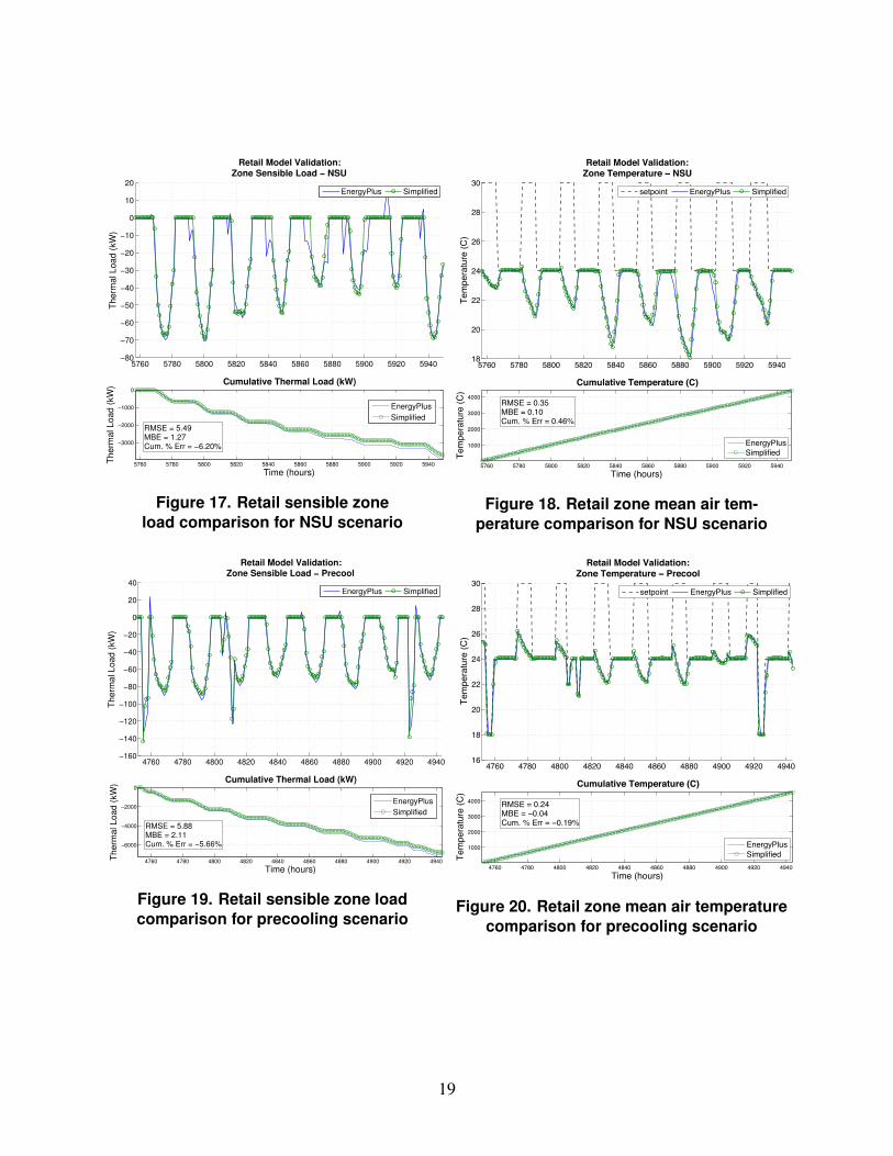
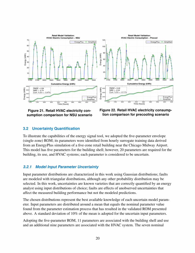
5760 5780 5800 5820 5840 5860 5880 5900 5920 59400
10
20
30
40
50
60
70
Energ
y (k
Wh)
Retail Model ValidationHVAC Electric Consumption NSU
EnergyPlus Simplified
5760 5780 5800 5820 5840 5860 5880 5900 5920 59400
1000
2000
3000
4000
Cumulative Energy (kWh)
Time (hours)
Energ
y (k
Wh)
RMSE = 494MBE = 074Cum Err = 347
EnergyPlusSimplified
4760 4780 4800 4820 4840 4860 4880 4900 4920 49400
20
40
60
80
100
120
Energ
y (k
Wh)
Retail Model ValidationHVAC Electric Consumption Precool
EnergyPlus Simplified
4760 4780 4800 4820 4840 4860 4880 4900 4920 49400
2000
4000
6000
Cumulative Energy (kWh)
Time (hours)
Energ
y (k
Wh)
RMSE = 649MBE = 004Cum Err = 011
EnergyPlusSimplified
Figure 21 Retail HVAC electricity con- Figure 22 Retail HVAC electricity consumpshysumption comparison for NSU scenario tion comparison for precooling scenario
32 Uncertainty Quantification
To illustrate the capabilities of the energy signal tool we adopted the five-parameter envelope (single-zone) ROM its parameters were identified from hourly surrogate training data derived from an EnergyPlus simulation of a five-zone retail building near the Chicago Midway Airport This model has five parameters for the building shell however 20 parameters are required for the building its use and HVAC systems each parameter is considered to be uncertain
321 Model Input Parameter Uncertainty
Input parameter distributions are characterized in this work using Gaussian distributions faults are modeled with triangular distributions although any other probability distribution may be selected In this work uncertainties are known varieties that are correctly quantified by an energy analyst using input distributions of choice faults are effects of unobserved uncertainties that affect the measured building performance but not the modeled predictions
The chosen distributions represent the best available knowledge of each uncertain model paramshyeter Input parameters are distributed around a mean that equals the nominal parameter value found from the parameter estimation process that has resulted in the validated ROM presented above A standard deviation of 10 of the mean is adopted for the uncertain input parameters
Adopting the five-parameter ROM 11 parameters are associated with the building shell and use and an additional nine parameters are associated with the HVAC system The seven nominal
20
building envelope parameters are shown in Table 3 the four use parameters are shown in Table 4 and the nine nominal HVAC-related model parameters are shown in Table 5
Table 4 Retail Building Use Parameters
Parameter Value Units
Lighting power density 3230 Wm2
Equipment power density 523 Wm2
Occupant density 71 m2per Infiltration flow rate 39 m3s
Table 5 Retail Building HVAC Parameters
Parameter Value Units
Supply fan efficiency 57 Maximum supply fan airflow 135 m3s Supply fan pressure rise 883 Pa DX coil rated capacity 319 kW DX coil rated sensible heat ratio 70 DX coil rated coefficient of performance (COP) 32 shyDX coil rated air mass flow rate 160 kgs Gas heating coil-rated capacity 457 kW Gas heating coil efficiency 80
To demonstrate the tool five of the 20 input parameters are considered uncertain lighting power density equipment power density occupant density DX coil-rated COP and gas heating coil efficiency The remaining 15 input parameters are taken at their nominal values In reality most of these 20 parameters would be uncertain at different levels of uncertainty
322 Operational and Equipment Faults
In spite of an energy analystrsquos best intentions and a belief that the model accurately reflects the building with all uncertainties undetected faults may affect building performance In this work a fault differs from a parameter uncertainty in that it is present without the knowledge of the energy analyst or building operator ie it is unobserved yet still affects the measured conditional distributions of building energy end use
We chose an additional six model parameters to represent such a faulted state Tehse are modeled by triangular distributions which may be asymmetrical The outdoor air fractionrsquos nominal value is 245 but may vary from 0 to 100 The airside economizer high limit temperature is nominally 28C but can vary between 12 and 40C Essentially at very low values of the
21
high limit temperature the economizer is disabled at high values the economizer operation is not overridden Heating and cooling temperature set points may differ from their assumed values with a random offset from -15 to +15 K Moreover the internal gains schedules may be expanded by up to 3 hours or contracted by up to 3 hours from the nominal building operation schedule Finally the schedules for internal gains from lighting and equipment may be shifted by up to 4 hours in each direction ie to earlier and later onsets Because the environment uses hourly time steps the schedule contractionexpansion and shift are rounded to the nearest full hour For the fault-free scenario the six fault parameters are kept at their nominal values For the faulted case all six fault parameters are randomly perturbed concurrently ie a very wide range of fault combinations is explored
Table 6 Fault Ranges
Parameter Nominal Minimum Maximum Units
Outdoor air fraction 245 0 100 Airside economizer high limit Cooling temperature set point Heating temperature set point Internal gains contractionexpansion Internal gains shift
28 228 217 10
800 am to 600 pm
12 -15 -15 -3 -4
40 +15 +15 + 3 + 4
C C C h h
Random sampling of 10000 annual samples for each case is presented here Because parameter combinations randomly drawn from the input distributions described above may lead to infeashysible model configurations for which no solution can be computed only valid model results are retained The sample rejection was put in place to deal with parameter combinations that cause simulation errors such as non-convergence and subsequent crashes Crashes are most often obshyserved when randomly sampling a wide range of HVAC equipment-rated parameters because the random sampling may not always produce physically consistent rated conditions Thus we expect that the wider the input parameter distributions the more frequently invalid model results are generated In the fault-free scenario 9994 of all samples were valid (six of 10000 failed) in the faulted scenario 9988 of all samples were valid (12 of 10000 failed)
The resultant conditional distribution of whole-building HVAC lighting (LTG) and plug elecshytricity EQP consumption is shown in Figure 23 Table 7 shows pertinent statistics of the same in units of [MWha] In the figure and table whole-building electricity (WBE) please define and add to nomenclature is the sum of HVAC LTG and miscellaneous electric loads EQP For fault-free and faulted cases the table shows the mean 10th 50th (median) and 90th percentiles along with the deterministic mean without consideration of any parameter uncertainty
It is evident that the uncertainty associated with the five selected parameters only slightly affects the mean but strongly affects the variance in the whole-building and submetered end uses The central 80 of the WBE consumption can be found within -7 and +8 from the determinisshytic mean in the fault-free case and within -24 and +20 from the deterministic mean in the
22
faulted case The influence of faults is stronger in the HVAC and LTG end uses compared to the EQP end use Given the dominance of HVAC and LTG end uses on whole-building consumption WBE faults strongly affect WBE as well Above all faults widen the energy distributions
100 200 300 400 500 600 7000
0005
001
0015
002
Prob
abilit
y
Whole Building Electric (MWh)50 100 150 200 250
0
002
004
006
008
Prob
abilit
y
HVAC Electric (MWh)
50 100 150 200 250 300 350 400 4500
0005
001
0015
002
Prob
abilit
y
Light Electric (MWh)10 20 30 40 50 60 70 80
0
002
004
006
008
01
Prob
abilit
y
Plug Electric (MWh)
FaultminusFreeFaulted
Figure 23 Distributions of whole-building HVAC lighting and plug electricity consumption
Table 7 Summary Statistics of Conditional Distributions of Whole-Building HVAC Lighting and Plug Electricity Consumption in [] in [MWha]
Percentile End-Use Case Mean 10th 50th 90th
WBE Deterministic 4163 Fault-free 100 93 100 108 Faulted 99 76 99 120
HVAC deterministic 1565 Fault-free 100 96 100 105 Faulted 96 79 97 112
LTG deterministic 2158 Fault-free 100 87 100 113 Faulted 100 71 99 130
EQP deterministic 441 Fault-free 100 87 100 113 Faulted 100 78 100 123
23
33 Decision Analysis
Comparing monitored data against a probable range of expected energy use is more insightful than comparing against a single number because it allows a building owner to assess the urgency of corrective actions that need to be taken If the measured energy use lies at the edge of the probable range of expected values given all the uncertainties in the model inputs the owner can be very confident that an issue requires attention In this work a decision-making tool was developed based on the probability distribution of model predictions to determine the expected utility of a range of available decisions suggesting the one that maximizes the expected utility The tool takes on the form of a modified traffic light with red yellow and green lights We adopted the perspective that a red light is shown both for high levels of overconsumption and high levels of underconsumption because a building consuming significantly less energy than expected may indicate an operational problem as significant as a building consuming too much A yellow signal is similarly used for cases of mild overconsumption and mild underconsumption A green light is reserved for measured building energy consumption that is in line with model expectations
As a first step a distribution of the model-predicted energy consumption (called Emod) was generated using Monte Carlo simulation as described in Section 32
Second the cases falling on the 5th median and 95th percentiles of the modeled energy distrishybutions were selected to represent low medium and high estimates of actual measured energy consumption (called Emeas) for fault-free and faulted scenarios The decision analysis compared the distribution of model-predicted energy consumption with Emeas to determine appropriate actions thus to illustrate the decision tool these three values of Emeas were taken from the samshypled distributions When physically implemented the measured energy consumption would be determined directly from building metering data
Third boundaries were computed from the measured energy consumption to define meaningful ranges of low and high levels of deviation in energy consumption Beginning with a low level of deviation let us define E0low such that it is Xlow percent below Emeas and E1low such that it is Xlow percent above Emeas
E0low = Emeas(1 minus Xlow)
E1low = Emeas(1 + Xlow)
Similarly for a high level of deviation letrsquos define E0high such that it is Xhigh percent below Emeas and E1high such that it is Xhigh percent above Emeas
E0high = Emeas(1 minus Xhigh)
E1high = Emeas(1 + Xhigh)
Of course Xlow lt Xhigh and we arbitrarily define Xlow to be 5 and Xhigh to be 10 ie a small deviation around the metered end use is plusmn5 and a large deviation plusmn10 It would be easy to adopt different values for Xlow and Xhigh for each building energy end use depending on its
24
temporal variability Once we have a conditional probability distribution of expected energy consumptions in hand we can make various kinds of statements Here we desire to report that the actual energy use is much higher somewhat higher similar somewhat lower or much lower than anticipated We further want to assign costs to making correct and incorrect statements and report the statement that has lowest expected cost
Fourth the empirical cumulative distribution of expected energy consumption was used to find the cumulative probabilities for the anticipated energy consumption to be below E0high (called P1) between E0high and E0low (called P2) between E0low and E1low (called P3) between E1low and E1high (called P4) and above E1high (called P5) Together these probabilities form the state probability vector PP = (P1P2P3P4P5)
T as shown in Figure 24
Figure 24 Relationship between deviation threshshyolds Xlow and Xhigh and state probability vector PP
Fifth we define a cost function K where cost is a function of state and action with a finite numshyber of states and a finite number of actions Therefore this cost function can be represented as a matrix Let us agree that there is one row per action and one column per state K(i j) ie cost of action i in state j Let action i = 1 display the lower red light (RL) on the modified traffic signal action i = 2 the lower yellow (YL) signal i = 3 a green (G) signal action i = 4 the upper yellow (YH) signal and finally i = 5 be displaying the upper red (RH) light Let j = 1 be the state that the model predicts a much lower (ML) energy consumption j = 2 a somewhat lower (SL) energy consumption j = 3 about the same (S) j = 4 a somewhat higher (SH) energy consumption and j = 5 a much higher (MH) energy consumption than the actual building Action vector Pa has thus five elements
25
Table 8 Decision Analysis State and Action
State j Anticipated Model Energy
Action i Much Lower Somewhat Lower Similar Somewhat Higher Much higher
Lower red Lower yellow Central green Upper yellow Upper red
K(RLML) K(YLML) K(GML)
K(YHML) K(RHML)
K(RLSL) K(YLSL) K(GSL)
K(YHSL) K(RHSL)
K(RLS) K(YLS) K(GS)
K(YHS) K(RHS)
K(RLSH) K(YLSH) K(GSH)
K(YHSH) K(RHSH)
K(RLMH) K(YLMH) K(GMH)
K(YHMH) K(RHMH)
An advantage of the presented decision analysis tool lies in its ability to individually set the costs of actions given certain states Here we make reasonable but somewhat arbitrary assumptions on the values of the cost matrix elements Showing an RL light when the model predicts ML energy consumption is assumed to have a cost of 4 (strong false negative lost savings opportunity) when the model predicts an SL energy consumption a cost of 3 (false negative) when the model predicts a similar energy consumption a cost of 2 (weak false negative) when the model predicts an SH energy consumption a cost of 1 (weak false negative) and finally when the model predicts MH energy consumption a cost of 0 (correct identification) Showing an RH light when the model predicts ML energy consumption is assumed to have a cost of 0 (correct identification) when the model predicts an SL energy consumption a cost of 1 (weak false positive) when the model predicts a similar energy consumption a cost of 2 (weak false positive) when the model predicts an SH energy consumption a cost of 3 (false positive) and finally when the model predicts MH energy consumption a cost of 4 (strong false positive unnecessary alarm) Similar arguments can be made for the remaining signals of a lower yellow (YL) a green and an upper yellow (YH) light and we yield the following cost matrix
⎡ K(RLML) K(RLSL) K(RLS) K(RLSH) K(RLMH)
⎤
K =
⎢⎢⎢⎢⎣
K(Y LML) K(GML)
K(Y HML) K(RHML)
K(Y LSL) K(GSL)
K(Y HSL) K(RHSL)
K(Y LS) K(GS)
K(Y HS) K(RHS)
K(Y LSH) K(GSH)
K(Y HSH) K(RHSH)
K(Y LMH) K(GMH)
K(Y HMH) K(RHMH)
⎥⎥⎥⎥⎦
⎡4 3 2 1 0
⎤
=
⎢⎢⎢⎢⎣
3 2 1 0
2 1 0 1
1 0 1 2
0 1 2 3
1 2 3 4
⎥⎥⎥⎥⎦ (37)
The expected cost vector for each action is found by multiplying the cost matrix K with the probability vector PP
E(Pa) = K middot PP
26
⎡ E (RL)
⎤ ⎡ K(RLML) K(RLSL) K(RLS) K(RL SH) K(RLMH)
⎤⎡P1⎤
E (Y L) K(Y LML) K(Y LSL) K(Y LS) K(Y LSH) K(Y LMH) P2⎢ ⎥ ⎢ ⎥⎢ ⎥⎢E (G)
⎥= ⎢
K(G ML) K(GSL) K(GS) K(GSH) K(GMH) ⎥⎢
P3⎥⎢ ⎥ ⎢ ⎥⎢ ⎥⎢
E (Y H)⎥ ⎢
K(Y HML) K(Y H SL) K(Y HS) K(Y HSH) K(Y HMH)⎥⎢
P4⎥⎣ ⎦ ⎣ ⎦⎣ ⎦
E (RH) K(RHML) K(RH SL) K(RHS) K(RHSH) K(RHMH) P5 ⎡ K(RLML)P1 + K(RLSL)P2 + K(RLS)P3 + K(RLSH)P4 + K(RLMH)P5
⎤
K(Y LML)P1 + K(Y LSL)P2 + K(Y LS)P3 + K(Y LSH)P4 + K(Y L MH)P5⎢ ⎥
= K(GML)P1 + K(GSL)P2 + K(GS)P3 + K(GSH)P4 + K(GMH)P5 (38)⎢⎢ ⎥⎥⎢
K(Y HML)P1 + K(Y HSL)P2 + K(Y H S)P3 + K(Y HSH)P4 + K(Y HMH)P5⎥⎣ ⎦
K(RHML)P1 + K(RHSL)P2 + K(RH S)P3 + K(RHSH)P4 + K(RHMH)P5
As suggested by utility theory the last step is to select the best action aopt in the face of uncershytainty ie activate that light which minimizes the expected cost
aopt = argminE(Pa)i
34 Bayesian Updating
Thus far the distributions of the uncertain model parameters were assumed to be Gaussian with a standard deviation equal to a fixed fraction of the parameter mean here 10 The choice of these distributions was made somewhat arbitrarily before any operational data was available from the actual building performance and termed before data because of its consideration prior to observation We believe that building performance measurements collected over an extended time period (ie after data) can be used to infer improved input parameter distributions by applying probability theory in general and Bayesrsquo theorem in particular See Jaynes (Jaynes 2003) for full development of Bayesian probability A brief explanation is provided below for information pertinent to this research
High-dimensional integrals associated with problems in computational physics lead to the develshyopment of Markov Chain Monte Carlo algorithms which can efficiently sample from probability distributions by exploiting the Markov property This has led to the explosion of Bayesian techshyniques with the Metropolis Algorithm as the breakthrough approach (named as one of the top 10 algorithms of the 20th century) (Cipra 2000) A probabilistic perspective not only provides insight into the relationship between sets of model parameters revealing tradeoffs and compenshysating interactions but also lends itself to a continuous model uncertainty quantification and tuning where the posterior distribution of an initial parameter estimate can be used as the prior for a subsequent parameter estimation update once new building performance data have been collected
Dodier used Bayesian (belief) networks for whole-building energy diagnostics (Dodier and Kreishyder 1999 Dodier et al 1998) Lauret et al (2006) demonstrated improvements over traditional parameter estimation methods by applying Bayesrsquo theorem to determine better estimates of conshyvection coefficients for a radiant barrier roof system model More recently Booth et al (2012)
27
used London housing stock models for hierarchical modeling with considerations of internal heating set points fraction of space heating air leakage heating system COP window U-value and window-to-wall ratio
In this work the Bayesian inference of uncertain model parameters relies on the extension of a previously developed technique (Neumann et al 2011) It has benefits over traditional methods because prior knowledge of the system can be directly incorporated into the estimation task and methods for addressing sensor noise are inherent to the Bayesian approach The inference can essentially be thought of as fitting a joint probability distribution to a measured dataset Specifishycally conditional probabilities are related through the product rule to derive Bayesrsquo theorem and allow consideration of before data and after data states of knowledge The prior probability distribution is updated with any measured data to form the posterior probability distribution which represents the state of knowledge in any inference task We propose a periodic process where model input parameter distributions are updated daily weekly monthly or for a similar period of interest As new measurements become available data effectively shape the distribution of expected building energy use according to the information gleaned from a combination of prior knowledge and sensor data uncertainty is still present but should decrease with additional data and understanding of the relationships among variables
The probability of parameter set Θ given measured data D and knowledge of the system K can be written as posterior probability p(Θ|DK) Bayesrsquo theorem then allows the conditional probability p(Θ|DK) to be computed from p(Θ|K) p(D|ΘK) and p(D|K) as shown in Equation 39
p(D|ΘK)p(Θ|DK) = p(Θ|K) (39)
p(D|K)
where p(Θ|K) represents prior knowledge about parameter values p(D|ΘK) represents the likeshylihood of observing the measured dataset D given a particular parameter set Θ and knowledge of the system K and p(D|K) is the probability of observing the dataset Ignoring the reference to system knowledge K the relation can be written in alternate form where the numerator reshymains the product of likelihood and prior and the denominator is a normalization factor so that posterior probabilities sum to unity
p(Θ)p(D|Θ)p(Θ|D) = (310)
sum p(Θi)p(D|Θi) i
Assuming random Gaussian noise about a measured datum Di the likelihood of an observation can be determined from its location within the normal distribution with standard deviation σε this is not in nomenclature centered at micro equal to the measured datum
p(Di|Θ) = radic 1
exp(minus(Di minus Mi)
2 ) (311)
σε 2π 2σε2
where Mi is the model output given the parameter set Θ
28
Further assuming independent errors the likelihood is that the entire dataset is simply the prodshyuct of the likelihoods of all individual points The assumption is likely valid for common HVAC sensors (eg temperature probes) but correlated errors could be handled with a slightly different formulation that is indicative of a fault model Measurement errors are often correlated because of for example hysteresis error or linearity error If such correlated errors are of concern a Bayesian (or other probabilistic) method may be used that can accommodate correlated measureshyments This work nonetheless assumes uncorrelated energy consumption measurements thus it ignores autocorrelation of errors which is estimated to be small For the dynamics and time range considered in this problem model structure is considered more important with respect to data fit than noise correlation From this model assumption we derive the easily computable likelihood function given by Equation 312
The likelihood function is maximized when the exponential term is minimized which occurs as the modeled data approach the measured (or surrogate) data When uniform priors are used with Equation 312 in a Bayesian calibration context the most likely parameters are equivalent to those that would be found using a least squares approach because the exponential term in Equation 312 is essentially the sum of squared errors (Pavlak et al 2014)
minus1 n
1 2p(D|Θ) = radic n exp sum (Di minus Mi) (312)
2σ2-σε 2π ε i=1
Evaluating Equation 312 directly can pose numerical issues because a small range of σε values results in a large range of likelihoods Double precision computing environments are typically capable of evaluating floating point numbers on the order of 10minus308 to 10308 This means that when using 3 weeks of hourly data (ie n = 504) σε must approximately be in the range of [0115] Values outside this range will cause the likelihood (and consequently the posterior) to evaluate to Inf NaN or 0 regardless of the time series fit These numerical issues can be alleviated by computing the natural logarithm of the posterior rather than the posterior directly (Lauret et al 2006 Sivia and Skilling 2006)
To compute the natural log of the posterior first the log of both sides of Equation 310 is taken ⎛ ⎞
p(Θ)p(D|Θ)ln(p(Θ|D)) = ln (313)⎝
sum p(Θi)p(D|Θi)⎠
i
The right-hand side of Equation 313 can be separated using logarithm product and quotient rules
ln(p(Θ|D)) = ln(p(Θ)) + ln(p(D|Θ)) minus ln sum p(Θi)p(D|Θi) (314)
i
29
The log-likelihood term of Equation 314
n1 minus1 2ln(p(D|Θ)) = ln radic n exp sum (Di minus Mi) (315) -σε 2π 2σε
2i=1
can be further simplified by applying product and quotient rules as shown in Equations 316 and 317 respectively
n1 minus1 2ln (p(D|Θ)) = ln radic n + ln exp sum (Di minus Mi) (316) -σε 2π 2σε
2i=1
radic nminus1 2ln(p(D|Θ)) = ln(1) minus ln ((
σε 2π
)n)+ ln exp sum (Di minus Mi) (317)
2σ2ε i=1
With ln(1) = 0 and the power rule can be applied to the middle term of the right-hand side The last term of the right-hand side simplifies because of to logarithmic identity to produce Equation 318
radic nminus1ln(p(D|Θ)) = minusn ln
(σε 2π
)+ sum (Di minus Mi)
2 (318)2σ2
ε i=1
Recombining the simplified log-likelihood of Equation 318 with the log-posterior equation of Equation 314 yields
radic n1 2ln(p(Θ|D)) = ln(p(Θ)) minus n ln(
σε 2π
)minus sum (Di minus Mi) (319)
2σ2ε i=1
minus ln sum p(Θi)p(D|Θi) i
The last term of the right-hand side of Equation 319 is ultimately a constant number subtracted from each individual ln(p(Θi)p(D|Θi)) value Because the value of this constant term does not impact the shape or relative information of the posterior it could be thought of as an arbitrary constant C
radic n1 2ln(p(Θ|D)) = ln(p(Θ)) minus n ln(
σε 2π
)minus sum (Di minus Mi) +C (320)
2σ2ε i=1
The constant term can be moved to the left-hand side of the equation producing Equation 321
radic n1 2ln(p(Θ|D)) minusC = ln(p(Θ)) minus n ln(
σε 2π
)minus sum (Di minus Mi) (321)
2σ2ε i=1
30
Because the objective is to avoid numerical underflow or overflow prescribing
C = max radic
ln(p(Θ)) minus n ln(
σε 2π
) minus
1 n
sum 2(Di minus Mi) (322)2σε
2i=1
shifts all points so that the maximum is 0 A maximum value of 0 in the ln space ensures that all values will be mapped to the interval [01] when taking the exponential After taking exponenshytials the values can be scaled by a constant so that probabilities sum to unity
The σε value is a noise term with physical interpretation Here there are three energy signals of interest HVAC lighting and equipmentndashall electrical terms with the error associated with minor fluctuations not incorporated in the physical model As previously stated prescribing an appropriate σε is necessary to prevent underflow or overflow which causes the inference task to crash from numerical issues The most appropriate σε value can be found by maximum a posteriori (MAP) estimation MAP is used to obtain a point estimate of σε by placing a prior distribution over σε and finding the maximum posterior mode according to the empirical data Because the HVAC lighting and equipment energy signals are considered independent in this study the MAP estimate of σε HVAC σε LT G and σε EQP were performed separately with a uniform prior on each σε set between 0 and 15 of the magnitude of the full individual signals
With the appropriate and optimal σε set for each signal it was then possible to calculate the probability of observing various energy signals as a function of the uncertainty parameters Because the signals are considered independent the joint probability of the building state is a product of the individual probabilities
p =prodpi = pHVAC pLT G pEQP (323) i
With the joint posterior probability distribution available from the equation above it was then possible to sample from the posterior directly or marginalize over all parameters not of interest and form a new prior That is the updating process is prior rarr posterior rarr prior The optimal updating period is a function of the building energy dynamics and available data
31
4 Results
Results are presented that (1) exemplify the decision support aspect of the tool and (2) illustrate the updating of the uncertain model parameters based on measured data
41 Decision Support Case Studies
The decision analysis results presented here are separated into fault-free and faulted scenarios In the fault-free scenario the high medium and low consumption values (surrogates of measured building energy consumption) are drawn from the conditional energy consumption distributions without faults and the decision analysis is based on the same distribution In contrast in the faulted scenario the high medium and low consumption values are drawn from the conditional energy consumption distributions including faults and the decision analysis is based on the distribution excluding faults
The results are shown as a matrix of figures The first row shows the whole-building electricity WBE consumption results for the last year then last month then last week followed by the last day The second row shows the HVAC energy consumption results for the time periods the third row shows the lighting LTG results and lastly the fourth row shows the EQP results Each of the 16 figure panels reveals a box plot1 Larger and smaller values respectively are shown as outliers of the expected energy consumption value for the time period of interest a diamond marker superimposed on the box plot to indicate the surrogate actual consumption value Emeas and on the left margin the energy signal tool with the signal chosen for the resultant cumulative probabilities PP cost matrix C and deviation thresholds Xlow and Xhigh The central green light separates cases of mild (YH) and strong (RH) overconsumption above the green light from the cases of of mild (YL) and strong (RL) underconsumption below the green light The particular traffic signal-inspired design is one of many possible designs chosen for illustration here thus many other valid designs can be conceived Moreover the planned field implementation of this energy signal tool would likely not show the box plots but only the signals Finally if only whole-building energy WBE measurements are available the tool would reveal only the top row of WBE versus the four time periods In contrast when submetering of HVAC LTG and EQP is available the lower three rows would be shown and the top WBE row omitted because it would not offer additional insight
1Box plots shown in this report adopt the common notation that the box occupies the interquartile range (IQR) from the lower (25th percentile) to the upper (75th percentile) The whiskers extend to the minimum and maximum values if these are less than 15 times the IQR below the lower or 15 times the IQR above the upper quartile
32
411 Fault-Free Scenario
4111 High Energy Consumption Case
Beginning on August 30 with the high energy consumption case at the 95th percentile a mild overconsumption is shown for all time scales for WBE and HVAC LTG and EQP show strong overconsumption for all time scales
350
400
450
500
WBEYear
MWh
35
40
45
50
55
WBEMonth
MWh
8
9
10
11
12
WBEWeek
MWh
1100
1200
1300
1400
1500
1600
1700
WBEDay
kWh
140
150
160
170
180
HVACYear
MWh
18
20
22
24
26
28
HVACMonth
MWh
4
45
5
55
6
HVACWeek
MWh
500
550
600
650
700
750
HVACDay
kWh
150
200
250
300
LTGYear
MWh
12
14
16
18
20
22
24
LTGMonth
MWh
3
35
4
45
5
55
LTGWeek
MWh
500
600
700
800
900
LTGDay
kWh
30
35
40
45
50
55
60
EQPYear
MWh
25
3
35
4
45
5
EQPMonth
MWh
06
07
08
09
1
11
EQPWeek
MWh
80
100
120
140
160
EQPDay
kWh
Figure 25 Fault-free high consumption case beginning August 30 (meashysured consumption data are indicated by diamonds in each figure)
4112 Medium Energy Consumption Case
The medium consumption cases for August and February show consistency between WBE HVAC and LTG green lights are shown for all time scales and the EQP consumption is low Because the EQP contribution to the total is small the WBE signal is not swayed to show a low yellow light
33
350
400
450
500
WBEYear
MWh
35
40
45
50
55
WBEMonth
MWh
8
9
10
11
12
WBEWeek
MWh
1100
1200
1300
1400
1500
1600
1700
WBEDay
kWh
140
150
160
170
180
HVACYear
MWh
18
20
22
24
26
28
HVACMonth
MWh
4
45
5
55
6
HVACWeek
MWh
500
550
600
650
700
750
HVACDay
kWh
150
200
250
300
LTGYear
MWh
12
14
16
18
20
22
24
LTGMonth
MWh
3
35
4
45
5
55
LTGWeek
MWh
500
600
700
800
900
LTGDay
kWh
30
35
40
45
50
55
60
EQPYear
MWh
25
3
35
4
45
5
EQPMonth
MWh
06
07
08
09
1
11
EQPWeek
MWh
80
100
120
140
160
EQPDay
kWh
Figure 26 Fault-free medium consumption case beginning August 30 (measured consumption data are indicated by diamonds in each figure)
4113 Low Energy Consumption Case
In the low consumption case it is interesting to note that the WBE signal shows a strong unshyderconsumption (low red) driven by the corresponding LTG signal even though HVAC conshysumption is similar to the model expectation (green) and EQP is only a mild underconsumption This case reveals the importance of submetering Without it it would not have been possible to isolate that LTG causes the warning HVAC could be ignored and EQP could be given less consideration
34
350
400
450
500
WBEYear
MWh
35
40
45
50
55
WBEMonth
MWh
8
9
10
11
12
WBEWeek
MWh
1100
1200
1300
1400
1500
1600
1700
WBEDay
kWh
140
150
160
170
180
HVACYear
MWh
18
20
22
24
26
28
HVACMonth
MWh
4
45
5
55
6
HVACWeek
MWh
500
550
600
650
700
750
HVACDay
kWh
150
200
250
300
LTGYear
MWh
12
14
16
18
20
22
24
LTGMonth
MWh
3
35
4
45
5
55
LTGWeek
MWh
500
600
700
800
900
LTGDay
kWh
30
35
40
45
50
55
60
EQPYear
MWh
25
3
35
4
45
5
EQPMonth
MWh
06
07
08
09
1
11
EQPWeek
MWh
80
100
120
140
160
EQPDay
kWh
Figure 27 Fault-free low consumption case beginning August 30 (meashysured consumption data are indicated by diamonds in each figure)
412 Faulted Scenarios
In the faulted scenarios the three cases are drawn from much wider distributions as shown in Figure 23
4121 High Energy Consumption Case
The high consumption case for August 30 shows consistency between WBE HVAC and LTG RH lights are shown for all time scales and the EQP consumption is close to model expectation However because the EQP contribution to the total is small the WBE signal is not swayed to show a low green light
35
350
400
450
500
WBEYear
MWh
35
40
45
50
55
WBEMonth
MWh
8
9
10
11
12
WBEWeek
MWh
1100
1200
1300
1400
1500
1600
1700
WBEDay
kWh
140
150
160
170
180
HVACYear
MWh
18
20
22
24
26
28
HVACMonth
MWh
4
45
5
55
6
HVACWeek
MWh
500
550
600
650
700
750
HVACDay
kWh
150
200
250
300
LTGYear
MWh
12
14
16
18
20
22
24
LTGMonth
MWh
3
35
4
45
5
55
LTGWeek
MWh
500
600
700
800
900
LTGDay
kWh
30
35
40
45
50
55
60
EQPYear
MWh
25
3
35
4
45
5
EQPMonth
MWh
06
07
08
09
1
11
EQPWeek
MWh
80
100
120
140
160
EQPDay
kWh
Figure 28 Faulted high consumption case beginning August 30 (meashysured consumption data are indicated by diamonds in each figure)
4122 Medium Energy Consumption Case
On an annual basis the medium consumption case leads to the expected green lights On time scales of months and shorter we can observe HVAC mild and strong underconsumption
36
350
400
450
500
WBEYear
MWh
35
40
45
50
55
WBEMonth
MWh
8
9
10
11
12
WBEWeek
MWh
1100
1200
1300
1400
1500
1600
1700
WBEDay
kWh
140
150
160
170
180
HVACYear
MWh
18
20
22
24
26
28
HVACMonth
MWh
4
45
5
55
6
HVACWeek
MWh
500
550
600
650
700
750
HVACDay
kWh
150
200
250
300
LTGYear
MWh
12
14
16
18
20
22
24
LTGMonth
MWh
3
35
4
45
5
55
LTGWeek
MWh
500
600
700
800
900
LTGDay
kWh
30
35
40
45
50
55
60
EQPYear
MWh
25
3
35
4
45
5
EQPMonth
MWh
06
07
08
09
1
11
EQPWeek
MWh
80
100
120
140
160
EQPDay
kWh
Figure 29 Faulted medium consumption case beginning August 30 (measured consumption data are indicated by diamonds in each figure)
4123 Low Energy Consumption Case
The low consumption case at the 5th percentile of the faulted distribution shows a consistent RL light for all end uses and time scales independent of season
37
300
350
400
450
500
WBEYear
MWh
35
40
45
50
55
WBEMonth
MWh
7
8
9
10
11
12
WBEWeek
MWh
1000
1100
1200
1300
1400
1500
1600
1700
WBEDay
kWh
130
140
150
160
170
180
HVACYear
MWh
18
20
22
24
26
28
HVACMonth
MWh
4
45
5
55
6
HVACWeek
MWh
500
550
600
650
700
750
HVACDay
kWh
150
200
250
300
LTGYear
MWh
12
14
16
18
20
22
24
LTGMonth
MWh
3
35
4
45
5
55
LTGWeek
MWh
500
600
700
800
900
LTGDay
kWh
30
35
40
45
50
55
60
EQPYear
MWh
25
3
35
4
45
5
EQPMonth
MWh
06
07
08
09
1
11
EQPWeek
MWh
80
100
120
140
160
EQPDay
kWh
Figure 30 Faulted low consumption case beginning August 30 (meashysured consumption data are indicated by diamonds in each figure)
Finally we present a sample illustration of how such a decision analysis tool would be deployed in the management of distributed commercial buildings Imagine a building operator is responsishyble for the energy-efficient operation of four buildings in a city Building 1 appears to be healthy all end uses show green signals for all four time scales building 2 suffers from overconsumption problems in the HVAC system that manifest themselves in the last day week and month buildshying 3 exhibits underconsumption in LTG especially during the last week which could speak to failed light sources or delamping measures not yet accounted for in the model finally building 4 suffers from multiple symptoms overconsumption in HVAC and EQP and underconsumption in LTG
38
Figure 31 Example of four buildings managed by a building operator
42 Bayesian Parameter Updating Case Studies
Results related to the probabilistic inference and updating of the uncertain model parameters are presented for September 21 at which point measurements over the past 30 days are used to update the five input parameter distributions that are deemed uncertain The high consumption case representing the 95th percentile of the fault-free conditional distributions is used to compute the likelihood functions for HVAC LTG and EQP for each of the nearly 10000 parameter
39
combinations Based on the simplifying assumptions articulated above we can then find the marginal posterior distribution for each selected uncertain parameter Please note that white Gaussian noise with a signal-to-noise ratio of 25 was added to the time series data of the high consumption case to simulate common measurement noise affecting building measurements Recent work by the same authors has shown the Bayesian inference approach to be robust with respect to a wide range of signal-to-noise ratios and noise colors (Pavlak et al 2014)
Table 9 shows the nominal values used to generate the prior input parameter distributions as well as the parameter values associated with the low medium and high cases investigated in this section The latter represent the ground truth values that will be compared to the posterior distributions for each model parameter to determine whether the measured data are used to update our belief of the uncertain parameters in a way that is consistent with the ground truth data
The table shows that several individual parameters appear inconsistent with the case they beshylong to As one example in the low consumption case the DX coil-rated COP is 31 which is below the nominal value One would expect a higher COP to be associated with the low conshysumption case However given the tradeoffs between lighting and equipment power consumption and the efficiency of the cooling equipment the low consumption case at the 5th percentile of 10000 simulation runs was the result of a less efficient RTU with strongly reduced lighting and equipment power densities The median consumption case resulted from a slightly higher lighting power density lower equipment power density lower occupant density and higher RTU COP all relative to the nominal values The high consumption case at the 95th percentile of all cases is characterized by higher lighting equipment and occupancy densities and lower HVAC equipment efficiency In this case of higher consumption the individual parameter values are all consistent with the theme of the case
Later sections discuss that whatever tradeoffs were at play in leading to the low medium and high cases the Bayesian parameter updating process is changing the posterior parameter disshytributions toward the ground truth values that form the basis of the measured (here surrogate) consumption data To that effect each of the following figures 32 to 46 shows the sampled prior distribution of the uncertain parameter as blue bars the sampled posterior distribution as red bars and the ground truth value that formed the basis of the surrogate measured data as a green vertical line
Gas heating efficiency should have no impact on electricity consumption thus increased electricshyity consumption should be independent from gas heating coil efficiency All the figures showing gas heating efficiency distributions illustrate that the gas heating efficiency posterior distribution is being smeared out ie becoming less informative because the evidence used in the likelihood function does not offer any clear clues about how to shape the posterior Although we show the prior and posterior distributions for gas heating efficiency for all three cases the independence of electricity consumption from gas heating efficiency is seen in a widening posterior in each case
40
Table 9 Building Model Truth Parameters
Parameter Nominal Low Medium High Units
Lighting power density 3230 2699 3309 3615 Wm2
Equipment power density 523 492 496 594 Wm2
Occupant density 0141 0149 0137 0151 perm2
DX coil rated COP 320 310 339 294 -Gas heating coil efficiency 80 74 70 77
421 High Energy Consumption Case
Figures 32 through 36 clearly illustrate how the measured data would be harnessed to update our belief about the uncertain parameters Each figure shows the empirical prior distribution as blue bars the empirical posterior distribution is shown as red bars Where the two distributions overlap a darker purple hue appears As stated above in the high energy consumption case all individual building parameter truth values are consistent with the theme of high energy conshysumption Lighting and equipment power density posteriors move to higher values relative to the nominal values that served as the mean of the normal prior distributions and gravitate toward the truth values (green vertical lines) used to generate the surrogate measured data Similarly occupancy densities in people per square meter are also slightly higher and the DX coil-rated COP is significantly lower than the nominal value gravitating toward the truth values Thus the Bayesian inference learns the truth values that form the basis of the measured data
Figure 32 Lighting power density prior (blue) and posterior (red) distributions on
September 21 based on past 30 days of high energy consumption Truth
value is shown as a green vertical line
Figure 33 Equipment power density prior (blue) and posterior (red) distribushytions on September 21 based on past 30 days of high energy consumption Truth value is shown as a green vertical line
41
Figure 34 Occupant density prior (blue) and posterior (red) distributions on
September 21 based on past 30 days of high energy consumption Truth
value is shown as a green vertical line
Figure 35 DX Coil Rated COP prior (blue) and posterior (red) distributions on
September 21 based on past 30 days of high energy consumption Truth
value is shown as a green vertical line
Figure 36 Gas heating coil efficiency prior (blue) and posterior (red) distributions on September 21 based on past 30 days of high energy consumption Truth value is shown as a green vertical line
422 Medium Energy Consumption Case
Figures 37 through 41 show how in the medium consumption case the data reveal the tradeoffs that form the basis of the medium consumption case A slightly higher lighting power density is compensated for by a significantly lower equipment power density because these two have the identical effects of adding convective internal gains to the sensible energy balance paired with slightly higher COPs Occupant density distribution has not materially changed from prior
42
to posterior in the medium consumption case As in the high consumption case the posterior distributions (except for gas heating efficiency as explained above) have moved in the direction of the truth values that form the foundation of the surrogate measured data
Figure 37 Lighting power density prior (blue) and posterior (red) distributions
on September 21 based on past 30 days of medium energy consumption Truth value is shown as a green vertical line
Figure 38 Equipment power density prior (blue) and posterior (red) distributions
on September 21 based on past 30 days of medium energy consumption Truth value is shown as a green vertical line
Figure 39 Occupant density prior (blue) and posterior (red) distributions on
September 21 based on past 30 days of medium energy consumption Truth value is shown as a green vertical line
Figure 40 DX Coil Rated COP prior (blue) and posterior (red) distributions on
September 21 based on past 30 days of medium energy consumption Truth value is shown as a green vertical line
43
Figure 41 Gas heating coil efficiency prior (blue) and posterior (red) distributions on September 21 based on past 30 days of medium
energy consumption Truth value is shown as a green vertical line
423 Low Energy Consumption Case
Figures 42 through 46 again clearly illustrate how the measured data would be harnessed to update our belief about the uncertain parameters In the low consumption case the data suggest significantly lower lighting and equipment power densities although occupant density seems to materially impact the measured data which lead to a virtually unchanged posterior
As shown in Table 9 the truth value of the DX coil-rated COP is slightly lower than the nominal value which is opposite to the theme of lower energy consumption As explained above the slightly inferior COP is more than compensated for by significantly lower lighting and equipment power densities The posterior COP distribution is close2 to the prior but slightly less than it feels like something is missing here suggesting that the Bayesian inference has learned the truth value
As before electricity consumption should not and does not have informative power for gas heating efficiency leaving the posterior smeared out relative to the prior
2A very heuristic visual interpretation of close was used We simply encourage the reader to determine in which direction the posterior distribution mass has been moving to the left to the right or virtually unchanged relative to the prior distribution In particular the point of using such loose language is to avoid comparing the empirical prior and posterior distributions with a more rigorous metric such as the maximum distance of the two cumulative distribution functions as used in the two-sample Kolmogorov-Smirnof test Future work will look into more rigorous metrics to automate the update process The point we wanted to make in this work however is that evidence is collected and used to inform updates of the input parameter distributions
44
Figure 42 Lighting power density prior (blue) and posterior (red) distributions
on September 21 based on past 30 days of low energy consumption Truth value is shown as a green vertical line
Figure 44 Occupant density prior (blue) and posterior (red) distributions on
September 21 based on past 30 days of low energy consumption Truth
value is shown as a green vertical line
Figure 43 Equipment power density prior (blue) and posterior (red) distribushytions on September 21 based on past 30 days of low energy consumption Truth value is shown as a green vertical line
Figure 45 DX Coil Rated COP prior (blue) and posterior (red) distributions
on September 21 based on past 30 days of low energy consumption Truth value is shown as a green vertical line
45
Figure 46 Gas heating coil efficiency prior (blue) and posterior (red) distributions on September 21 based on past 30 days of low
energy consumption Truth value is shown as a green vertical line
46
5 Summary and Conclusions
A prototype energy signal tool was demonstrated for operational whole-building and system-level energy performance assessment The purpose of the tool is to give an assessment that a building operator or other user can quickly comprehend Toward this end the energy signal tool estimates energy use for various end uses from a low-order lumped-parameter model taking into account uncertainty (via a Monte Carlo method) in model parameters and inputs The result of the modelshying phase is a probability distribution over estimated energy use The range of estimated energy use is divided into intervals based on the observed energy use and the probability that energy use is in an interval is computed as the mass of the estimated energy use distribution in that interval An indicator (traffic light color) is chosen to minimize misclassification cost Model parameter distributions are adjusted over time via Bayesian updating
The experimental study investigated whole-building energy signal accuracy in the presence of uncertainty and faults at the submetered level which may lead to tradeoffs at the whole-building level that are not detectable without submetering Submetering of end uses is recommended to avoid confounding underconsumption and overconsumption among various end uses An examshyple of four building energy signal displays is offered to illustrate energy performance features that could be detected by the energy signal tool The Bayesian inference results presented show that observations can be used to periodically update model parameter distributions and that the posterior distributions indeed gravitate toward the ground truth parameter values that formed the basis of the surrogate measured data We presented results for a 30-day learning cycle
Future improvements in the inference process would eliminate the assumptions of temporal independence of subsequent observations of a particular variable and structural independence of multiple observed variables Accounting for covariance among observed variables will help to better attribute observations to individual model parameters
47
Bibliography
Attia S Gratia E Herde AD Hensen JL (2012) ldquoSimulation-based decision support tool for early stages of zero-energy building designrdquo Energy and Buildings 49(0) pp 2 ndash 15
Augenbroe G Castro D Ramkrishnan K (2009) ldquoDecision model for energy performance improvements in existing buildingsrdquo Journal of Engineering Design and Technology 7(1) pp 21 ndash 36
Balcomb J Curtner A (2000) ldquoMulti-criteria decision-making process for buildingsrdquo Energy Conversion Engineering Conference and Exhibit Vol 1 pp 528 ndash 535 Las Vegas NV USA IEEE
Basso N Garavaglia E Sgambi L Imagawa N (2013) Natural hazards vs Decision-making processes in buildings life cycle management New York NY USA CRC Press
Bauermann K Spiecker S Weber C (3 2014) ldquoIndividual decisions and system development Integrating modelling approaches for the heating marketrdquo Applied Energy 116 pp 149ndash158
Booth A Choudhary R Spiegelhalter D (Feb 2012) ldquoHandling uncertainty in housing stock modelsrdquo Building and Environment 48(0) pp 35ndash47
Bracken C Rajagopalan B Prairie J (Mar 2010) ldquoA multisite seasonal ensemble streamflow forecasting techniquerdquo Water Resources Research 46(3) pp 1ndash12 URL httpdoiwileycom1010292009WR007965
Brandemuehl M Shauna G Inger A (1993) ldquoHVAC2 Toolkit Algorithms and Subroutines for Secondary HVAC System Energy Calculationsrdquo ASHRAE Atlanta GA
Braun JE Chaturvedi N (2002) ldquoAn inverse gray-box model for transient building load predictionrdquo HVACampR Research 8(1) pp 73ndash100
Burkhart MC Heo Y Zavala VM (2014) ldquoMeasurement and verification of building systems under uncertain data A Gaussian process modeling approachrdquo Energy and Buildings 75 pp 189 ndash 198
Chaturvedi N Braun J Bernhard R (2000) Analytical Tools for Dynamic Building Conshytrol Implementation of Thermal Storage in Building Mass American Society of Heating Refrigerating and Air-Conditioning Engineers
Choi JH Aziz A Loftness V (2009) ldquoDecision support for improving occupant environmenshytal satisfaction in office buildings The relationship between sub-set of IEQ satisfaction and overall environmental satisfactionrdquo Ninth International Conference of Healthy Buildings p 747 Syracuse NY USA
48
Cipra BA (2000) ldquoThe best of the 20th century Editors name top 10 algorithmsrdquo SIAM news 33(4) pp 1ndash2
Crawley DB Lawrie LK Winkelmann FC Buhl WF Huang YJ Pedersen CO Strand RK Liesen RJ Fisher DE Witte MJ et al (2001) ldquoEnergyPlus creating a new-generation building energy simulation programrdquo Energy and Buildings 33(4) pp 319ndash331
Das S Chew M Poh KL (2010) ldquoMulti-criteria decision analysis in building maintainability using analytical hierarchy processrdquo Construction Management and Economics 28(10) pp 1043 ndash 1056
De Farias C Soares H Pirmez L Delicato F Santos I Carmo LF De Souza J Zomaya A Dohler M (2014) ldquoA control and decision system for smart buildings using wireless sensor and actuator networksrdquo European Transactions on Telecommunications 25(1) pp 120 ndash 135
De Wit S Augenbroe G (2002) ldquoAnalysis of uncertainty in building design evaluations and its implicationsrdquo Energy and Buildings 34(9) pp 951 ndash 958
Deru M Field K Studer D Benne K Griffith B Torcellini P Halverson M Winiarski D Liu B Rosenberg M Huang J Yazdanian M Crawley D (2010) US Department of Energy Commercial Reference Building Models of the National Building Stock Washington DC US Department of Energy Energy Efficiency and Renewable Energy Office of Building Technologies
Diakaki C Grigoroudis E Kabelis N Kolokotsa D Kalaitzakis K Stavrakakis G (2010) ldquoA multi-objective decision model for the improvement of energy efficiency in buildingsrdquo Energy 35(12) pp 5483 ndash 5496
Diakaki C Grigoroudis E Kolokotsa D (2013) ldquoPerformance study of a multi-objective mathematical programming modelling approach for energy decision-making in buildingsrdquo Energy 59 pp 534 ndash 542
Dodier R Kreider J (1999) ldquoWhole Building Energy Diagnosticsrdquo ASHRAE Trans 105(1) pp 579ndash589
Dodier RH Curtiss PS Kreider JF (1998) ldquoSmall-scale on-line diagnostics for an HVAC systemrdquo Transactions-American Society Of Heating Refrigerating And Air Conditioning Engineers 104 pp 530ndash539
DOE U (2010) ldquoEnergyPlus Engineering Referencerdquo The Reference to EnergyPlus Calculashytions URL httpapps1eereenergygovbuildingsenergypluspdfs engineeringreferencepdf
49
Filippoupolitis A Gelenbe E (2009) ldquoA decision support system for disaster management in buildingsrdquo Summer Computer Simulation Conference pp 141 ndash 147 Society for Modeling amp Simulation International
Florita AR Brackney LJ Otanicar TP Robertson J (2013) ldquoClassification of Commercial Building Electrical Demand Profiles for Energy Storage Applicationsrdquo Journal of Solar Energy Engineering 135(3) p 031020
Gulbinas R Jain RK Taylor JE (2014) ldquoBizWatts A modular socio-technical energy management system for empowering commercial building occupants to conserve energyrdquo Applied Energy In-Press
Gultekin P Anumba CJ Leicht RM (2013) ldquoTowards an integrated process model and decision support system for high performance green retrofitsrdquo Architectural Engineering Conference 2013 pp 912 ndash 923 State College PA United states
Heo Y Augenbroe G Choudhary R (2011) ldquoRisk analysis of energy-efficiency projects based on bayesian calibration of building energy modelsrdquo Twelth Conference of International Building Performance Simulation Association pp 2579 ndash 2586 Sydney AUS
Heo Y Zavala VM (2012) ldquoGaussian process modeling for measurement and verification of building energy savingsrdquo Energy and Buildings 53 pp 7 ndash 18
ISO E (2007) ldquo13790 2007rdquo Energy performance of buildings-Calculation of energy use for space heating and cooling
Jaynes ET (2003) Probability theory the logic of science Cambridge university press
Judkoff R Balcomb J Hancock C Barker G Subbarao K (2000) Side-By-Side Thermal Tests of Modular Offices A Validation Study of the STEM Method NREL Report TP-550shy23940 National Renewable Energy Laboratory
Judkoff R Wortman D OrsquoDoherty B Burch J (20081983) Methodology for Validating Building Energy Analysis Simulations NREL Report No TP-550-42059 National Renewable Energy Laboratory Golden CO
Kiluk S (11 2014) ldquoDynamic classification system in large-scale supervision of energy effishyciency in buildingsrdquo Applied Energy 132 pp 1ndash14
Kolokotsa D Diakaki C Grigoroudis E Stavrakakis G Kalaitzakis K (2009) ldquoDecishysion support methodologies on the energy efficiency and energy management in buildingsrdquo Advances in Building Energy Research 3(1) pp 121 ndash 146
Lauret P Miranville F Boyer H Garde F Adelard L (May 2006) ldquoBayesian parameter estimation of convective heat transfer coefficients of a roof-mounted radiant barrier systemrdquo Journal of Solar Energy Engineering 128 pp 213 ndash 225
50
Lee BD Sun Y Augenbroe G Paredis CJ (2013a) ldquoTowards better prediction of building performance A workbench to analyze uncertainty in building simulationrdquo Thirteenth Internashytional Conference of the International Building Performance Simulation Association pp 1231 ndash 1238 Chambery France
Lee SH Augenbroe G Lee JK Zhao F (2013b) ldquoA design methodology for energy infrastructures at the campus scalerdquo Computer-Aided Civil and Infrastructure Engineering 28(10) pp 753 ndash 768
Lee S Liu Y Chunduri S Solnosky RL Messner JI Leicht RM Anumba CJ (2012) ldquoDevelopment of a process model to support integrated design for energy efficient buildingsrdquo International Conference on Computing in Civil Engineering pp 261 ndash 268 Clearwater Beach FL USA
Li Z Heo Y Augenbroe G (2009) ldquoHVAC design informed by organizational simulationrdquo Eleventh International IBPSA Conference pp 2198 ndash 2203 Glasgow UK
Mohseni H Setunge S Zhang GM Wakefield R (2013) ldquoCondition monitoring and condition aggregation for optimised decision making in management of buildingsrdquo Applied Mechanics and Materials 438-439 pp 1719 ndash 1725
Moon HJ Augenbroe G (2008) ldquoEmpowerment of decision-makers in mould remediationrdquo Building Research and Information 36(5) pp 486 ndash 498
Neumann C Jacob D Burhenne S Florita A Burger E Schmidt F (2011) Model-Based Methods for Fault Detection and Optimization in Building Operations (Modellbasierte Methoden fuumlr die Fehlererkennung und Optimierung im Gebaumludebetrieb) Fraunhofer ISE
Pavlak G Florita A Henze G Rajagopalan B (2014) ldquoComparison of Traditional and Bayesian Calibration Techniques for Gray-Box Modelingrdquo Journal of Architectural Engineershying 20(2) p 04013011
Piotr R Laurence B Alison C Ahmed AS (2012) ldquoDecision making aid for selection of renewablesustainable energy systems for buildingsrdquo International Conference on Sustainable Design and Construction pp 306 ndash 313 Kansas City MO USA ASCE
Rafiq M (2000) ldquoImportance of Pareto optimum solutions in making informed decisions in engineering designrdquo Eighth International Conference on Computing in Civil and Building Engineering Vol 2 pp 1325 ndash 1333 Stanford CA USA ASCE
Sanctis GD Fischer K Kohler J Fontana M Faber M (2011) A probabilistic frameshywork for generic fire risk assessment and risk-based decision making in buildings Zurich Switzerland CRC Press
Seem J (1987) Modeling of heat transfer in buildings PhD Thesis University of Wisconsin-Madison
51
Sivia D Skilling J (2006) ldquoParameter estimation IIrdquo Data Analysis A Bayesian Tutorial Chap 3 pp 35 ndash 77 Oxford University Press
Subbarao K (1988a) PSTAR - Primary and Secondary Terms-Analysis and Renormalization A Unified Approach to Building and Energy Simulations and Short-Term Testing A Summary NREL Report TR-254-3347 National Renewable Energy Laboratory
mdashmdashmdash (1988b) PSTAR - Primary and Secondary Terms Analysis and Renormalization A Unified Approach to Building Energy Simulations and Short-Term Monitoring NREL Report TR-254-3175 National Renewable Energy Laboratory
Subbarao K Burch J Hancock C Lekov A Balcomb J (1988) Short-term Energy Monishytoring (STEM) Application of the PSTAR Method to a Residence in Fredericksburg Virginia NREL Report TR-254-3356 National Renewable Energy Laboratory
Subbarao K Mort D Burch J (1985) Short-Term Measurements for the Determination of Envelope Retrofit Performance NREL Report TP-253-2639 National Renewable Energy Laboratory
Sun Y Heo Y Tan M Xie H Jeff Wu C Augenbroe G (2014) ldquoUncertainty quantificashytion of microclimate variables in building energy modelsrdquo Journal of Building Performance Simulation 7(1) pp 17 ndash 32
Takizawa A Kawamura H Tani A (2000) ldquoSimulation of urban system ldquoas it could berdquo by multiagent modelrdquo Eighth International Conference on Computing in Civil and Building Engineering Vol 2 pp 1566 ndash 1573 Stanford CA USA ASCE
Thompson BP Bank LC (2010) ldquoUse of system dynamics as a decision-making tool in building design and operationrdquo Building and Environment 45(4) pp 1006 ndash 1015
Ugwu O Anumba C Newnham L Thorpe A (2000) ldquoAgent-oriented collaborative design of industrial buildingsrdquo Eighth International Conference on Computing in Civil and Building Engineering Vol 1 pp 333 ndash 340 Stanford CA USA ASCE
Vinh A (2009) ldquoComputer-based monitoring for decision support systems and disaster preshyparedness in buildingsrdquo Systemics Cybernetrics and Informatics 7 pp 51ndash56
Wang L Greenberg S Fiegel J Rubalcava A Earni S Pang X Yin R Woodworth S Hernandez-Maldonado J (2 2013) ldquoMonitoring-based HVAC commissioning of an existing office building for energy efficiencyrdquo Applied Energy 102 pp 1382ndash1390
Zeiler W Maaijen R Maassen W (2012) ldquoDecision support for sustainable healthier and more productive buildingsrdquo Tenth International Conference Healthy Buildings pp 1ndash6 Brisbane AUS
52
Zhao P Suryanarayanan S Simoes MG (2010) ldquoAn energy management system for building structures using a multi-agent decision-making control methodologyrdquo Industry Applications Society Annual Meeting pp 1ndash8 Houston TX USA IEEE
Zhao Y Wang S Xiao F (12 2013) ldquoPattern recognition-based chillers fault detection method using Support Vector Data Descriptionrdquo Applied Energy 112 pp 1041ndash1048
53
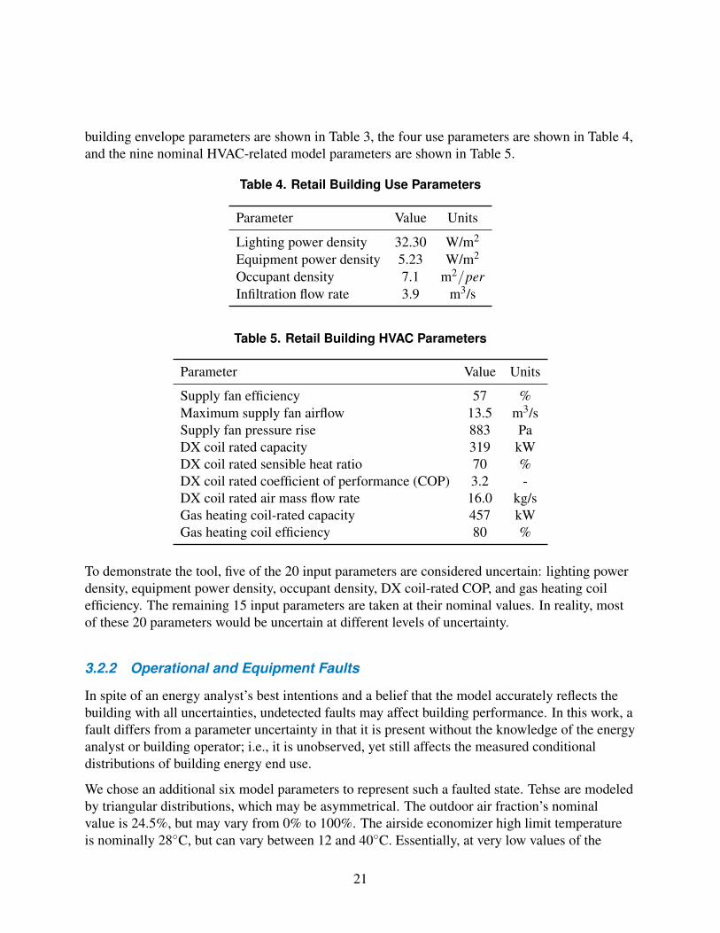
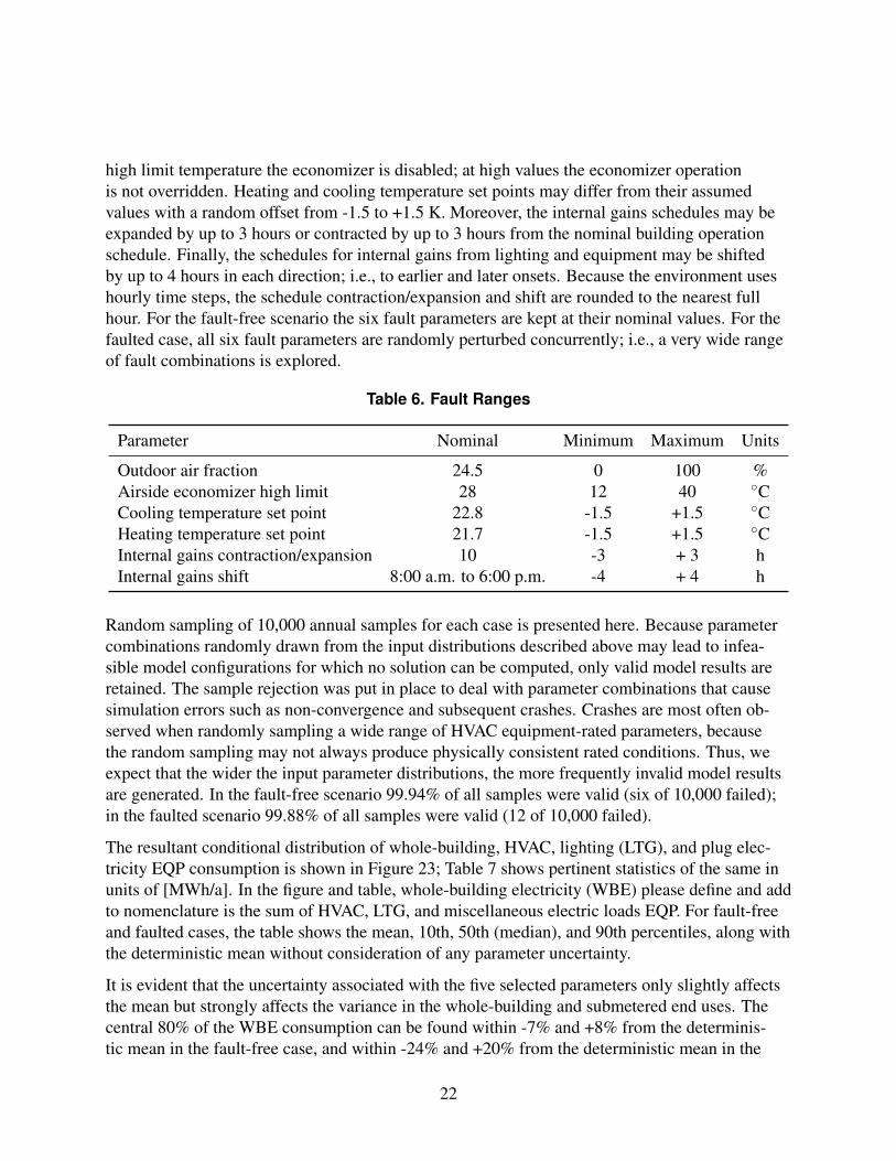
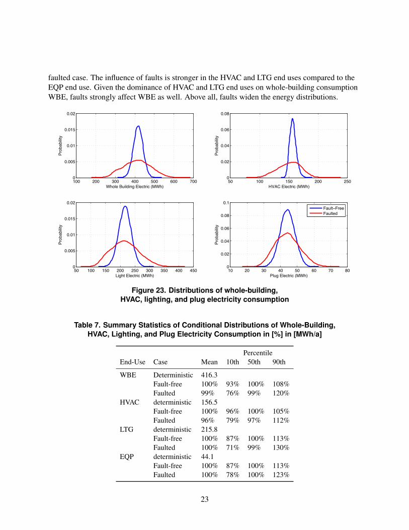
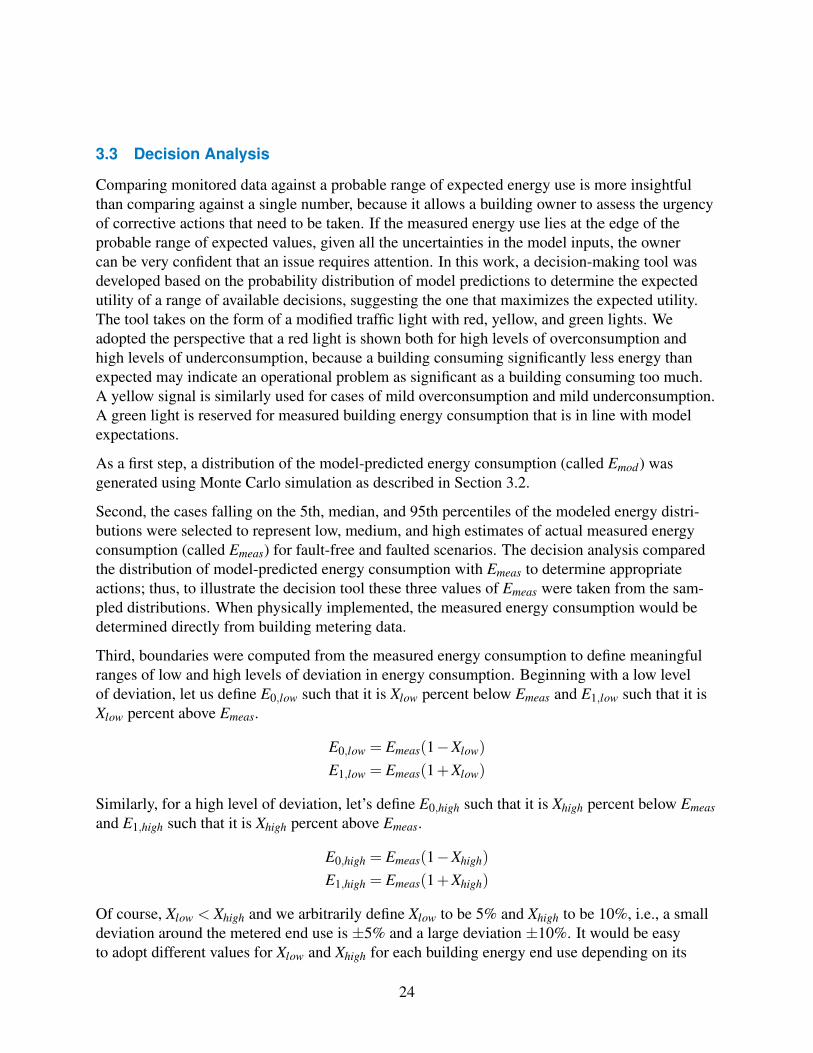
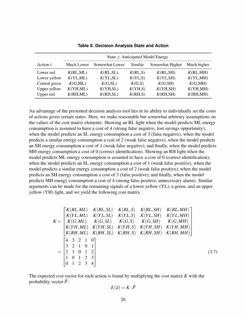
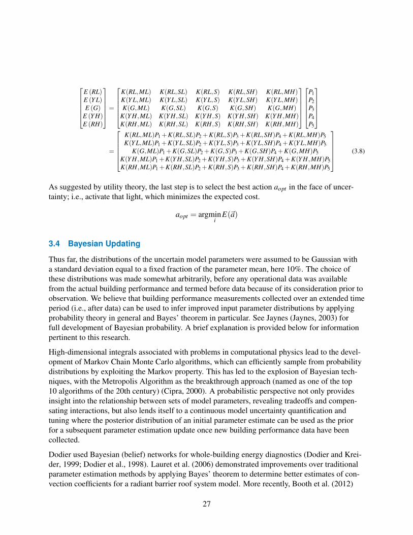
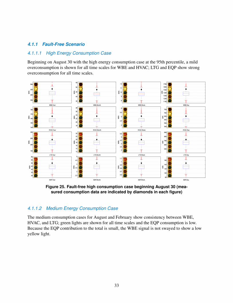
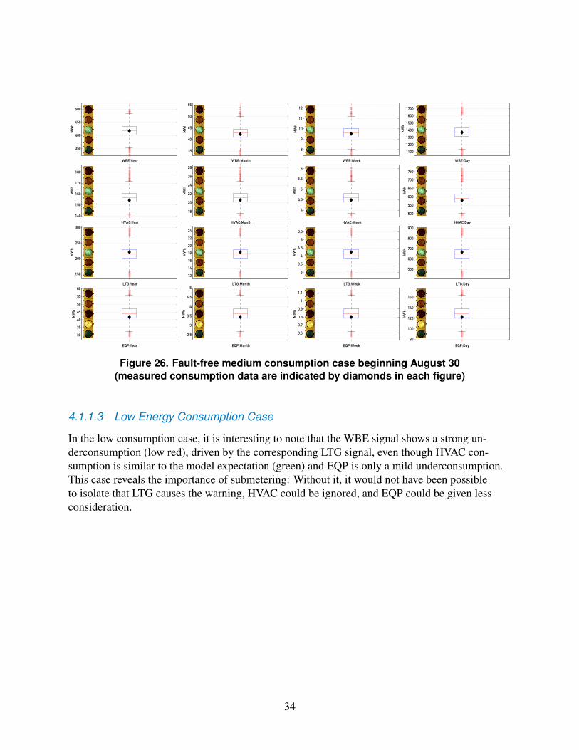
350
400
450
500
WBEYear
MWh
35
40
45
50
55
WBEMonth
MWh
8
9
10
11
12
WBEWeek
MWh
1100
1200
1300
1400
1500
1600
1700
WBEDay
kWh
140
150
160
170
180
HVACYear
MWh
18
20
22
24
26
28
HVACMonth
MWh
4
45
5
55
6
HVACWeek
MWh
500
550
600
650
700
750
HVACDay
kWh
150
200
250
300
LTGYear
MWh
12
14
16
18
20
22
24
LTGMonth
MWh
3
35
4
45
5
55
LTGWeek
MWh
500
600
700
800
900
LTGDay
kWh
30
35
40
45
50
55
60
EQPYear
MWh
25
3
35
4
45
5
EQPMonth
MWh
06
07
08
09
1
11
EQPWeek
MWh
80
100
120
140
160
EQPDay
kWh
Figure 26 Fault-free medium consumption case beginning August 30 (measured consumption data are indicated by diamonds in each figure)
4113 Low Energy Consumption Case
In the low consumption case it is interesting to note that the WBE signal shows a strong unshyderconsumption (low red) driven by the corresponding LTG signal even though HVAC conshysumption is similar to the model expectation (green) and EQP is only a mild underconsumption This case reveals the importance of submetering Without it it would not have been possible to isolate that LTG causes the warning HVAC could be ignored and EQP could be given less consideration
34
350
400
450
500
WBEYear
MWh
35
40
45
50
55
WBEMonth
MWh
8
9
10
11
12
WBEWeek
MWh
1100
1200
1300
1400
1500
1600
1700
WBEDay
kWh
140
150
160
170
180
HVACYear
MWh
18
20
22
24
26
28
HVACMonth
MWh
4
45
5
55
6
HVACWeek
MWh
500
550
600
650
700
750
HVACDay
kWh
150
200
250
300
LTGYear
MWh
12
14
16
18
20
22
24
LTGMonth
MWh
3
35
4
45
5
55
LTGWeek
MWh
500
600
700
800
900
LTGDay
kWh
30
35
40
45
50
55
60
EQPYear
MWh
25
3
35
4
45
5
EQPMonth
MWh
06
07
08
09
1
11
EQPWeek
MWh
80
100
120
140
160
EQPDay
kWh
Figure 27 Fault-free low consumption case beginning August 30 (meashysured consumption data are indicated by diamonds in each figure)
412 Faulted Scenarios
In the faulted scenarios the three cases are drawn from much wider distributions as shown in Figure 23
4121 High Energy Consumption Case
The high consumption case for August 30 shows consistency between WBE HVAC and LTG RH lights are shown for all time scales and the EQP consumption is close to model expectation However because the EQP contribution to the total is small the WBE signal is not swayed to show a low green light
35
350
400
450
500
WBEYear
MWh
35
40
45
50
55
WBEMonth
MWh
8
9
10
11
12
WBEWeek
MWh
1100
1200
1300
1400
1500
1600
1700
WBEDay
kWh
140
150
160
170
180
HVACYear
MWh
18
20
22
24
26
28
HVACMonth
MWh
4
45
5
55
6
HVACWeek
MWh
500
550
600
650
700
750
HVACDay
kWh
150
200
250
300
LTGYear
MWh
12
14
16
18
20
22
24
LTGMonth
MWh
3
35
4
45
5
55
LTGWeek
MWh
500
600
700
800
900
LTGDay
kWh
30
35
40
45
50
55
60
EQPYear
MWh
25
3
35
4
45
5
EQPMonth
MWh
06
07
08
09
1
11
EQPWeek
MWh
80
100
120
140
160
EQPDay
kWh
Figure 28 Faulted high consumption case beginning August 30 (meashysured consumption data are indicated by diamonds in each figure)
4122 Medium Energy Consumption Case
On an annual basis the medium consumption case leads to the expected green lights On time scales of months and shorter we can observe HVAC mild and strong underconsumption
36
350
400
450
500
WBEYear
MWh
35
40
45
50
55
WBEMonth
MWh
8
9
10
11
12
WBEWeek
MWh
1100
1200
1300
1400
1500
1600
1700
WBEDay
kWh
140
150
160
170
180
HVACYear
MWh
18
20
22
24
26
28
HVACMonth
MWh
4
45
5
55
6
HVACWeek
MWh
500
550
600
650
700
750
HVACDay
kWh
150
200
250
300
LTGYear
MWh
12
14
16
18
20
22
24
LTGMonth
MWh
3
35
4
45
5
55
LTGWeek
MWh
500
600
700
800
900
LTGDay
kWh
30
35
40
45
50
55
60
EQPYear
MWh
25
3
35
4
45
5
EQPMonth
MWh
06
07
08
09
1
11
EQPWeek
MWh
80
100
120
140
160
EQPDay
kWh
Figure 29 Faulted medium consumption case beginning August 30 (measured consumption data are indicated by diamonds in each figure)
4123 Low Energy Consumption Case
The low consumption case at the 5th percentile of the faulted distribution shows a consistent RL light for all end uses and time scales independent of season
37
300
350
400
450
500
WBEYear
MWh
35
40
45
50
55
WBEMonth
MWh
7
8
9
10
11
12
WBEWeek
MWh
1000
1100
1200
1300
1400
1500
1600
1700
WBEDay
kWh
130
140
150
160
170
180
HVACYear
MWh
18
20
22
24
26
28
HVACMonth
MWh
4
45
5
55
6
HVACWeek
MWh
500
550
600
650
700
750
HVACDay
kWh
150
200
250
300
LTGYear
MWh
12
14
16
18
20
22
24
LTGMonth
MWh
3
35
4
45
5
55
LTGWeek
MWh
500
600
700
800
900
LTGDay
kWh
30
35
40
45
50
55
60
EQPYear
MWh
25
3
35
4
45
5
EQPMonth
MWh
06
07
08
09
1
11
EQPWeek
MWh
80
100
120
140
160
EQPDay
kWh
Figure 30 Faulted low consumption case beginning August 30 (meashysured consumption data are indicated by diamonds in each figure)
Finally we present a sample illustration of how such a decision analysis tool would be deployed in the management of distributed commercial buildings Imagine a building operator is responsishyble for the energy-efficient operation of four buildings in a city Building 1 appears to be healthy all end uses show green signals for all four time scales building 2 suffers from overconsumption problems in the HVAC system that manifest themselves in the last day week and month buildshying 3 exhibits underconsumption in LTG especially during the last week which could speak to failed light sources or delamping measures not yet accounted for in the model finally building 4 suffers from multiple symptoms overconsumption in HVAC and EQP and underconsumption in LTG
38
Figure 31 Example of four buildings managed by a building operator
42 Bayesian Parameter Updating Case Studies
Results related to the probabilistic inference and updating of the uncertain model parameters are presented for September 21 at which point measurements over the past 30 days are used to update the five input parameter distributions that are deemed uncertain The high consumption case representing the 95th percentile of the fault-free conditional distributions is used to compute the likelihood functions for HVAC LTG and EQP for each of the nearly 10000 parameter
39
combinations Based on the simplifying assumptions articulated above we can then find the marginal posterior distribution for each selected uncertain parameter Please note that white Gaussian noise with a signal-to-noise ratio of 25 was added to the time series data of the high consumption case to simulate common measurement noise affecting building measurements Recent work by the same authors has shown the Bayesian inference approach to be robust with respect to a wide range of signal-to-noise ratios and noise colors (Pavlak et al 2014)
Table 9 shows the nominal values used to generate the prior input parameter distributions as well as the parameter values associated with the low medium and high cases investigated in this section The latter represent the ground truth values that will be compared to the posterior distributions for each model parameter to determine whether the measured data are used to update our belief of the uncertain parameters in a way that is consistent with the ground truth data
The table shows that several individual parameters appear inconsistent with the case they beshylong to As one example in the low consumption case the DX coil-rated COP is 31 which is below the nominal value One would expect a higher COP to be associated with the low conshysumption case However given the tradeoffs between lighting and equipment power consumption and the efficiency of the cooling equipment the low consumption case at the 5th percentile of 10000 simulation runs was the result of a less efficient RTU with strongly reduced lighting and equipment power densities The median consumption case resulted from a slightly higher lighting power density lower equipment power density lower occupant density and higher RTU COP all relative to the nominal values The high consumption case at the 95th percentile of all cases is characterized by higher lighting equipment and occupancy densities and lower HVAC equipment efficiency In this case of higher consumption the individual parameter values are all consistent with the theme of the case
Later sections discuss that whatever tradeoffs were at play in leading to the low medium and high cases the Bayesian parameter updating process is changing the posterior parameter disshytributions toward the ground truth values that form the basis of the measured (here surrogate) consumption data To that effect each of the following figures 32 to 46 shows the sampled prior distribution of the uncertain parameter as blue bars the sampled posterior distribution as red bars and the ground truth value that formed the basis of the surrogate measured data as a green vertical line
Gas heating efficiency should have no impact on electricity consumption thus increased electricshyity consumption should be independent from gas heating coil efficiency All the figures showing gas heating efficiency distributions illustrate that the gas heating efficiency posterior distribution is being smeared out ie becoming less informative because the evidence used in the likelihood function does not offer any clear clues about how to shape the posterior Although we show the prior and posterior distributions for gas heating efficiency for all three cases the independence of electricity consumption from gas heating efficiency is seen in a widening posterior in each case
40
Table 9 Building Model Truth Parameters
Parameter Nominal Low Medium High Units
Lighting power density 3230 2699 3309 3615 Wm2
Equipment power density 523 492 496 594 Wm2
Occupant density 0141 0149 0137 0151 perm2
DX coil rated COP 320 310 339 294 -Gas heating coil efficiency 80 74 70 77
421 High Energy Consumption Case
Figures 32 through 36 clearly illustrate how the measured data would be harnessed to update our belief about the uncertain parameters Each figure shows the empirical prior distribution as blue bars the empirical posterior distribution is shown as red bars Where the two distributions overlap a darker purple hue appears As stated above in the high energy consumption case all individual building parameter truth values are consistent with the theme of high energy conshysumption Lighting and equipment power density posteriors move to higher values relative to the nominal values that served as the mean of the normal prior distributions and gravitate toward the truth values (green vertical lines) used to generate the surrogate measured data Similarly occupancy densities in people per square meter are also slightly higher and the DX coil-rated COP is significantly lower than the nominal value gravitating toward the truth values Thus the Bayesian inference learns the truth values that form the basis of the measured data
Figure 32 Lighting power density prior (blue) and posterior (red) distributions on
September 21 based on past 30 days of high energy consumption Truth
value is shown as a green vertical line
Figure 33 Equipment power density prior (blue) and posterior (red) distribushytions on September 21 based on past 30 days of high energy consumption Truth value is shown as a green vertical line
41
Figure 34 Occupant density prior (blue) and posterior (red) distributions on
September 21 based on past 30 days of high energy consumption Truth
value is shown as a green vertical line
Figure 35 DX Coil Rated COP prior (blue) and posterior (red) distributions on
September 21 based on past 30 days of high energy consumption Truth
value is shown as a green vertical line
Figure 36 Gas heating coil efficiency prior (blue) and posterior (red) distributions on September 21 based on past 30 days of high energy consumption Truth value is shown as a green vertical line
422 Medium Energy Consumption Case
Figures 37 through 41 show how in the medium consumption case the data reveal the tradeoffs that form the basis of the medium consumption case A slightly higher lighting power density is compensated for by a significantly lower equipment power density because these two have the identical effects of adding convective internal gains to the sensible energy balance paired with slightly higher COPs Occupant density distribution has not materially changed from prior
42
to posterior in the medium consumption case As in the high consumption case the posterior distributions (except for gas heating efficiency as explained above) have moved in the direction of the truth values that form the foundation of the surrogate measured data
Figure 37 Lighting power density prior (blue) and posterior (red) distributions
on September 21 based on past 30 days of medium energy consumption Truth value is shown as a green vertical line
Figure 38 Equipment power density prior (blue) and posterior (red) distributions
on September 21 based on past 30 days of medium energy consumption Truth value is shown as a green vertical line
Figure 39 Occupant density prior (blue) and posterior (red) distributions on
September 21 based on past 30 days of medium energy consumption Truth value is shown as a green vertical line
Figure 40 DX Coil Rated COP prior (blue) and posterior (red) distributions on
September 21 based on past 30 days of medium energy consumption Truth value is shown as a green vertical line
43
Figure 41 Gas heating coil efficiency prior (blue) and posterior (red) distributions on September 21 based on past 30 days of medium
energy consumption Truth value is shown as a green vertical line
423 Low Energy Consumption Case
Figures 42 through 46 again clearly illustrate how the measured data would be harnessed to update our belief about the uncertain parameters In the low consumption case the data suggest significantly lower lighting and equipment power densities although occupant density seems to materially impact the measured data which lead to a virtually unchanged posterior
As shown in Table 9 the truth value of the DX coil-rated COP is slightly lower than the nominal value which is opposite to the theme of lower energy consumption As explained above the slightly inferior COP is more than compensated for by significantly lower lighting and equipment power densities The posterior COP distribution is close2 to the prior but slightly less than it feels like something is missing here suggesting that the Bayesian inference has learned the truth value
As before electricity consumption should not and does not have informative power for gas heating efficiency leaving the posterior smeared out relative to the prior
2A very heuristic visual interpretation of close was used We simply encourage the reader to determine in which direction the posterior distribution mass has been moving to the left to the right or virtually unchanged relative to the prior distribution In particular the point of using such loose language is to avoid comparing the empirical prior and posterior distributions with a more rigorous metric such as the maximum distance of the two cumulative distribution functions as used in the two-sample Kolmogorov-Smirnof test Future work will look into more rigorous metrics to automate the update process The point we wanted to make in this work however is that evidence is collected and used to inform updates of the input parameter distributions
44
Figure 42 Lighting power density prior (blue) and posterior (red) distributions
on September 21 based on past 30 days of low energy consumption Truth value is shown as a green vertical line
Figure 44 Occupant density prior (blue) and posterior (red) distributions on
September 21 based on past 30 days of low energy consumption Truth
value is shown as a green vertical line
Figure 43 Equipment power density prior (blue) and posterior (red) distribushytions on September 21 based on past 30 days of low energy consumption Truth value is shown as a green vertical line
Figure 45 DX Coil Rated COP prior (blue) and posterior (red) distributions
on September 21 based on past 30 days of low energy consumption Truth value is shown as a green vertical line
45
Figure 46 Gas heating coil efficiency prior (blue) and posterior (red) distributions on September 21 based on past 30 days of low
energy consumption Truth value is shown as a green vertical line
46
5 Summary and Conclusions
A prototype energy signal tool was demonstrated for operational whole-building and system-level energy performance assessment The purpose of the tool is to give an assessment that a building operator or other user can quickly comprehend Toward this end the energy signal tool estimates energy use for various end uses from a low-order lumped-parameter model taking into account uncertainty (via a Monte Carlo method) in model parameters and inputs The result of the modelshying phase is a probability distribution over estimated energy use The range of estimated energy use is divided into intervals based on the observed energy use and the probability that energy use is in an interval is computed as the mass of the estimated energy use distribution in that interval An indicator (traffic light color) is chosen to minimize misclassification cost Model parameter distributions are adjusted over time via Bayesian updating
The experimental study investigated whole-building energy signal accuracy in the presence of uncertainty and faults at the submetered level which may lead to tradeoffs at the whole-building level that are not detectable without submetering Submetering of end uses is recommended to avoid confounding underconsumption and overconsumption among various end uses An examshyple of four building energy signal displays is offered to illustrate energy performance features that could be detected by the energy signal tool The Bayesian inference results presented show that observations can be used to periodically update model parameter distributions and that the posterior distributions indeed gravitate toward the ground truth parameter values that formed the basis of the surrogate measured data We presented results for a 30-day learning cycle
Future improvements in the inference process would eliminate the assumptions of temporal independence of subsequent observations of a particular variable and structural independence of multiple observed variables Accounting for covariance among observed variables will help to better attribute observations to individual model parameters
47
Bibliography
Attia S Gratia E Herde AD Hensen JL (2012) ldquoSimulation-based decision support tool for early stages of zero-energy building designrdquo Energy and Buildings 49(0) pp 2 ndash 15
Augenbroe G Castro D Ramkrishnan K (2009) ldquoDecision model for energy performance improvements in existing buildingsrdquo Journal of Engineering Design and Technology 7(1) pp 21 ndash 36
Balcomb J Curtner A (2000) ldquoMulti-criteria decision-making process for buildingsrdquo Energy Conversion Engineering Conference and Exhibit Vol 1 pp 528 ndash 535 Las Vegas NV USA IEEE
Basso N Garavaglia E Sgambi L Imagawa N (2013) Natural hazards vs Decision-making processes in buildings life cycle management New York NY USA CRC Press
Bauermann K Spiecker S Weber C (3 2014) ldquoIndividual decisions and system development Integrating modelling approaches for the heating marketrdquo Applied Energy 116 pp 149ndash158
Booth A Choudhary R Spiegelhalter D (Feb 2012) ldquoHandling uncertainty in housing stock modelsrdquo Building and Environment 48(0) pp 35ndash47
Bracken C Rajagopalan B Prairie J (Mar 2010) ldquoA multisite seasonal ensemble streamflow forecasting techniquerdquo Water Resources Research 46(3) pp 1ndash12 URL httpdoiwileycom1010292009WR007965
Brandemuehl M Shauna G Inger A (1993) ldquoHVAC2 Toolkit Algorithms and Subroutines for Secondary HVAC System Energy Calculationsrdquo ASHRAE Atlanta GA
Braun JE Chaturvedi N (2002) ldquoAn inverse gray-box model for transient building load predictionrdquo HVACampR Research 8(1) pp 73ndash100
Burkhart MC Heo Y Zavala VM (2014) ldquoMeasurement and verification of building systems under uncertain data A Gaussian process modeling approachrdquo Energy and Buildings 75 pp 189 ndash 198
Chaturvedi N Braun J Bernhard R (2000) Analytical Tools for Dynamic Building Conshytrol Implementation of Thermal Storage in Building Mass American Society of Heating Refrigerating and Air-Conditioning Engineers
Choi JH Aziz A Loftness V (2009) ldquoDecision support for improving occupant environmenshytal satisfaction in office buildings The relationship between sub-set of IEQ satisfaction and overall environmental satisfactionrdquo Ninth International Conference of Healthy Buildings p 747 Syracuse NY USA
48
Cipra BA (2000) ldquoThe best of the 20th century Editors name top 10 algorithmsrdquo SIAM news 33(4) pp 1ndash2
Crawley DB Lawrie LK Winkelmann FC Buhl WF Huang YJ Pedersen CO Strand RK Liesen RJ Fisher DE Witte MJ et al (2001) ldquoEnergyPlus creating a new-generation building energy simulation programrdquo Energy and Buildings 33(4) pp 319ndash331
Das S Chew M Poh KL (2010) ldquoMulti-criteria decision analysis in building maintainability using analytical hierarchy processrdquo Construction Management and Economics 28(10) pp 1043 ndash 1056
De Farias C Soares H Pirmez L Delicato F Santos I Carmo LF De Souza J Zomaya A Dohler M (2014) ldquoA control and decision system for smart buildings using wireless sensor and actuator networksrdquo European Transactions on Telecommunications 25(1) pp 120 ndash 135
De Wit S Augenbroe G (2002) ldquoAnalysis of uncertainty in building design evaluations and its implicationsrdquo Energy and Buildings 34(9) pp 951 ndash 958
Deru M Field K Studer D Benne K Griffith B Torcellini P Halverson M Winiarski D Liu B Rosenberg M Huang J Yazdanian M Crawley D (2010) US Department of Energy Commercial Reference Building Models of the National Building Stock Washington DC US Department of Energy Energy Efficiency and Renewable Energy Office of Building Technologies
Diakaki C Grigoroudis E Kabelis N Kolokotsa D Kalaitzakis K Stavrakakis G (2010) ldquoA multi-objective decision model for the improvement of energy efficiency in buildingsrdquo Energy 35(12) pp 5483 ndash 5496
Diakaki C Grigoroudis E Kolokotsa D (2013) ldquoPerformance study of a multi-objective mathematical programming modelling approach for energy decision-making in buildingsrdquo Energy 59 pp 534 ndash 542
Dodier R Kreider J (1999) ldquoWhole Building Energy Diagnosticsrdquo ASHRAE Trans 105(1) pp 579ndash589
Dodier RH Curtiss PS Kreider JF (1998) ldquoSmall-scale on-line diagnostics for an HVAC systemrdquo Transactions-American Society Of Heating Refrigerating And Air Conditioning Engineers 104 pp 530ndash539
DOE U (2010) ldquoEnergyPlus Engineering Referencerdquo The Reference to EnergyPlus Calculashytions URL httpapps1eereenergygovbuildingsenergypluspdfs engineeringreferencepdf
49
Filippoupolitis A Gelenbe E (2009) ldquoA decision support system for disaster management in buildingsrdquo Summer Computer Simulation Conference pp 141 ndash 147 Society for Modeling amp Simulation International
Florita AR Brackney LJ Otanicar TP Robertson J (2013) ldquoClassification of Commercial Building Electrical Demand Profiles for Energy Storage Applicationsrdquo Journal of Solar Energy Engineering 135(3) p 031020
Gulbinas R Jain RK Taylor JE (2014) ldquoBizWatts A modular socio-technical energy management system for empowering commercial building occupants to conserve energyrdquo Applied Energy In-Press
Gultekin P Anumba CJ Leicht RM (2013) ldquoTowards an integrated process model and decision support system for high performance green retrofitsrdquo Architectural Engineering Conference 2013 pp 912 ndash 923 State College PA United states
Heo Y Augenbroe G Choudhary R (2011) ldquoRisk analysis of energy-efficiency projects based on bayesian calibration of building energy modelsrdquo Twelth Conference of International Building Performance Simulation Association pp 2579 ndash 2586 Sydney AUS
Heo Y Zavala VM (2012) ldquoGaussian process modeling for measurement and verification of building energy savingsrdquo Energy and Buildings 53 pp 7 ndash 18
ISO E (2007) ldquo13790 2007rdquo Energy performance of buildings-Calculation of energy use for space heating and cooling
Jaynes ET (2003) Probability theory the logic of science Cambridge university press
Judkoff R Balcomb J Hancock C Barker G Subbarao K (2000) Side-By-Side Thermal Tests of Modular Offices A Validation Study of the STEM Method NREL Report TP-550shy23940 National Renewable Energy Laboratory
Judkoff R Wortman D OrsquoDoherty B Burch J (20081983) Methodology for Validating Building Energy Analysis Simulations NREL Report No TP-550-42059 National Renewable Energy Laboratory Golden CO
Kiluk S (11 2014) ldquoDynamic classification system in large-scale supervision of energy effishyciency in buildingsrdquo Applied Energy 132 pp 1ndash14
Kolokotsa D Diakaki C Grigoroudis E Stavrakakis G Kalaitzakis K (2009) ldquoDecishysion support methodologies on the energy efficiency and energy management in buildingsrdquo Advances in Building Energy Research 3(1) pp 121 ndash 146
Lauret P Miranville F Boyer H Garde F Adelard L (May 2006) ldquoBayesian parameter estimation of convective heat transfer coefficients of a roof-mounted radiant barrier systemrdquo Journal of Solar Energy Engineering 128 pp 213 ndash 225
50
Lee BD Sun Y Augenbroe G Paredis CJ (2013a) ldquoTowards better prediction of building performance A workbench to analyze uncertainty in building simulationrdquo Thirteenth Internashytional Conference of the International Building Performance Simulation Association pp 1231 ndash 1238 Chambery France
Lee SH Augenbroe G Lee JK Zhao F (2013b) ldquoA design methodology for energy infrastructures at the campus scalerdquo Computer-Aided Civil and Infrastructure Engineering 28(10) pp 753 ndash 768
Lee S Liu Y Chunduri S Solnosky RL Messner JI Leicht RM Anumba CJ (2012) ldquoDevelopment of a process model to support integrated design for energy efficient buildingsrdquo International Conference on Computing in Civil Engineering pp 261 ndash 268 Clearwater Beach FL USA
Li Z Heo Y Augenbroe G (2009) ldquoHVAC design informed by organizational simulationrdquo Eleventh International IBPSA Conference pp 2198 ndash 2203 Glasgow UK
Mohseni H Setunge S Zhang GM Wakefield R (2013) ldquoCondition monitoring and condition aggregation for optimised decision making in management of buildingsrdquo Applied Mechanics and Materials 438-439 pp 1719 ndash 1725
Moon HJ Augenbroe G (2008) ldquoEmpowerment of decision-makers in mould remediationrdquo Building Research and Information 36(5) pp 486 ndash 498
Neumann C Jacob D Burhenne S Florita A Burger E Schmidt F (2011) Model-Based Methods for Fault Detection and Optimization in Building Operations (Modellbasierte Methoden fuumlr die Fehlererkennung und Optimierung im Gebaumludebetrieb) Fraunhofer ISE
Pavlak G Florita A Henze G Rajagopalan B (2014) ldquoComparison of Traditional and Bayesian Calibration Techniques for Gray-Box Modelingrdquo Journal of Architectural Engineershying 20(2) p 04013011
Piotr R Laurence B Alison C Ahmed AS (2012) ldquoDecision making aid for selection of renewablesustainable energy systems for buildingsrdquo International Conference on Sustainable Design and Construction pp 306 ndash 313 Kansas City MO USA ASCE
Rafiq M (2000) ldquoImportance of Pareto optimum solutions in making informed decisions in engineering designrdquo Eighth International Conference on Computing in Civil and Building Engineering Vol 2 pp 1325 ndash 1333 Stanford CA USA ASCE
Sanctis GD Fischer K Kohler J Fontana M Faber M (2011) A probabilistic frameshywork for generic fire risk assessment and risk-based decision making in buildings Zurich Switzerland CRC Press
Seem J (1987) Modeling of heat transfer in buildings PhD Thesis University of Wisconsin-Madison
51
Sivia D Skilling J (2006) ldquoParameter estimation IIrdquo Data Analysis A Bayesian Tutorial Chap 3 pp 35 ndash 77 Oxford University Press
Subbarao K (1988a) PSTAR - Primary and Secondary Terms-Analysis and Renormalization A Unified Approach to Building and Energy Simulations and Short-Term Testing A Summary NREL Report TR-254-3347 National Renewable Energy Laboratory
mdashmdashmdash (1988b) PSTAR - Primary and Secondary Terms Analysis and Renormalization A Unified Approach to Building Energy Simulations and Short-Term Monitoring NREL Report TR-254-3175 National Renewable Energy Laboratory
Subbarao K Burch J Hancock C Lekov A Balcomb J (1988) Short-term Energy Monishytoring (STEM) Application of the PSTAR Method to a Residence in Fredericksburg Virginia NREL Report TR-254-3356 National Renewable Energy Laboratory
Subbarao K Mort D Burch J (1985) Short-Term Measurements for the Determination of Envelope Retrofit Performance NREL Report TP-253-2639 National Renewable Energy Laboratory
Sun Y Heo Y Tan M Xie H Jeff Wu C Augenbroe G (2014) ldquoUncertainty quantificashytion of microclimate variables in building energy modelsrdquo Journal of Building Performance Simulation 7(1) pp 17 ndash 32
Takizawa A Kawamura H Tani A (2000) ldquoSimulation of urban system ldquoas it could berdquo by multiagent modelrdquo Eighth International Conference on Computing in Civil and Building Engineering Vol 2 pp 1566 ndash 1573 Stanford CA USA ASCE
Thompson BP Bank LC (2010) ldquoUse of system dynamics as a decision-making tool in building design and operationrdquo Building and Environment 45(4) pp 1006 ndash 1015
Ugwu O Anumba C Newnham L Thorpe A (2000) ldquoAgent-oriented collaborative design of industrial buildingsrdquo Eighth International Conference on Computing in Civil and Building Engineering Vol 1 pp 333 ndash 340 Stanford CA USA ASCE
Vinh A (2009) ldquoComputer-based monitoring for decision support systems and disaster preshyparedness in buildingsrdquo Systemics Cybernetrics and Informatics 7 pp 51ndash56
Wang L Greenberg S Fiegel J Rubalcava A Earni S Pang X Yin R Woodworth S Hernandez-Maldonado J (2 2013) ldquoMonitoring-based HVAC commissioning of an existing office building for energy efficiencyrdquo Applied Energy 102 pp 1382ndash1390
Zeiler W Maaijen R Maassen W (2012) ldquoDecision support for sustainable healthier and more productive buildingsrdquo Tenth International Conference Healthy Buildings pp 1ndash6 Brisbane AUS
52
Zhao P Suryanarayanan S Simoes MG (2010) ldquoAn energy management system for building structures using a multi-agent decision-making control methodologyrdquo Industry Applications Society Annual Meeting pp 1ndash8 Houston TX USA IEEE
Zhao Y Wang S Xiao F (12 2013) ldquoPattern recognition-based chillers fault detection method using Support Vector Data Descriptionrdquo Applied Energy 112 pp 1041ndash1048
53
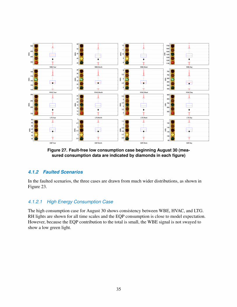
350
400
450
500
WBEYear
MWh
35
40
45
50
55
WBEMonth
MWh
8
9
10
11
12
WBEWeek
MWh
1100
1200
1300
1400
1500
1600
1700
WBEDay
kWh
140
150
160
170
180
HVACYear
MWh
18
20
22
24
26
28
HVACMonth
MWh
4
45
5
55
6
HVACWeek
MWh
500
550
600
650
700
750
HVACDay
kWh
150
200
250
300
LTGYear
MWh
12
14
16
18
20
22
24
LTGMonth
MWh
3
35
4
45
5
55
LTGWeek
MWh
500
600
700
800
900
LTGDay
kWh
30
35
40
45
50
55
60
EQPYear
MWh
25
3
35
4
45
5
EQPMonth
MWh
06
07
08
09
1
11
EQPWeek
MWh
80
100
120
140
160
EQPDay
kWh
Figure 27 Fault-free low consumption case beginning August 30 (meashysured consumption data are indicated by diamonds in each figure)
412 Faulted Scenarios
In the faulted scenarios the three cases are drawn from much wider distributions as shown in Figure 23
4121 High Energy Consumption Case
The high consumption case for August 30 shows consistency between WBE HVAC and LTG RH lights are shown for all time scales and the EQP consumption is close to model expectation However because the EQP contribution to the total is small the WBE signal is not swayed to show a low green light
35
350
400
450
500
WBEYear
MWh
35
40
45
50
55
WBEMonth
MWh
8
9
10
11
12
WBEWeek
MWh
1100
1200
1300
1400
1500
1600
1700
WBEDay
kWh
140
150
160
170
180
HVACYear
MWh
18
20
22
24
26
28
HVACMonth
MWh
4
45
5
55
6
HVACWeek
MWh
500
550
600
650
700
750
HVACDay
kWh
150
200
250
300
LTGYear
MWh
12
14
16
18
20
22
24
LTGMonth
MWh
3
35
4
45
5
55
LTGWeek
MWh
500
600
700
800
900
LTGDay
kWh
30
35
40
45
50
55
60
EQPYear
MWh
25
3
35
4
45
5
EQPMonth
MWh
06
07
08
09
1
11
EQPWeek
MWh
80
100
120
140
160
EQPDay
kWh
Figure 28 Faulted high consumption case beginning August 30 (meashysured consumption data are indicated by diamonds in each figure)
4122 Medium Energy Consumption Case
On an annual basis the medium consumption case leads to the expected green lights On time scales of months and shorter we can observe HVAC mild and strong underconsumption
36
350
400
450
500
WBEYear
MWh
35
40
45
50
55
WBEMonth
MWh
8
9
10
11
12
WBEWeek
MWh
1100
1200
1300
1400
1500
1600
1700
WBEDay
kWh
140
150
160
170
180
HVACYear
MWh
18
20
22
24
26
28
HVACMonth
MWh
4
45
5
55
6
HVACWeek
MWh
500
550
600
650
700
750
HVACDay
kWh
150
200
250
300
LTGYear
MWh
12
14
16
18
20
22
24
LTGMonth
MWh
3
35
4
45
5
55
LTGWeek
MWh
500
600
700
800
900
LTGDay
kWh
30
35
40
45
50
55
60
EQPYear
MWh
25
3
35
4
45
5
EQPMonth
MWh
06
07
08
09
1
11
EQPWeek
MWh
80
100
120
140
160
EQPDay
kWh
Figure 29 Faulted medium consumption case beginning August 30 (measured consumption data are indicated by diamonds in each figure)
4123 Low Energy Consumption Case
The low consumption case at the 5th percentile of the faulted distribution shows a consistent RL light for all end uses and time scales independent of season
37
300
350
400
450
500
WBEYear
MWh
35
40
45
50
55
WBEMonth
MWh
7
8
9
10
11
12
WBEWeek
MWh
1000
1100
1200
1300
1400
1500
1600
1700
WBEDay
kWh
130
140
150
160
170
180
HVACYear
MWh
18
20
22
24
26
28
HVACMonth
MWh
4
45
5
55
6
HVACWeek
MWh
500
550
600
650
700
750
HVACDay
kWh
150
200
250
300
LTGYear
MWh
12
14
16
18
20
22
24
LTGMonth
MWh
3
35
4
45
5
55
LTGWeek
MWh
500
600
700
800
900
LTGDay
kWh
30
35
40
45
50
55
60
EQPYear
MWh
25
3
35
4
45
5
EQPMonth
MWh
06
07
08
09
1
11
EQPWeek
MWh
80
100
120
140
160
EQPDay
kWh
Figure 30 Faulted low consumption case beginning August 30 (meashysured consumption data are indicated by diamonds in each figure)
Finally we present a sample illustration of how such a decision analysis tool would be deployed in the management of distributed commercial buildings Imagine a building operator is responsishyble for the energy-efficient operation of four buildings in a city Building 1 appears to be healthy all end uses show green signals for all four time scales building 2 suffers from overconsumption problems in the HVAC system that manifest themselves in the last day week and month buildshying 3 exhibits underconsumption in LTG especially during the last week which could speak to failed light sources or delamping measures not yet accounted for in the model finally building 4 suffers from multiple symptoms overconsumption in HVAC and EQP and underconsumption in LTG
38
Figure 31 Example of four buildings managed by a building operator
42 Bayesian Parameter Updating Case Studies
Results related to the probabilistic inference and updating of the uncertain model parameters are presented for September 21 at which point measurements over the past 30 days are used to update the five input parameter distributions that are deemed uncertain The high consumption case representing the 95th percentile of the fault-free conditional distributions is used to compute the likelihood functions for HVAC LTG and EQP for each of the nearly 10000 parameter
39
combinations Based on the simplifying assumptions articulated above we can then find the marginal posterior distribution for each selected uncertain parameter Please note that white Gaussian noise with a signal-to-noise ratio of 25 was added to the time series data of the high consumption case to simulate common measurement noise affecting building measurements Recent work by the same authors has shown the Bayesian inference approach to be robust with respect to a wide range of signal-to-noise ratios and noise colors (Pavlak et al 2014)
Table 9 shows the nominal values used to generate the prior input parameter distributions as well as the parameter values associated with the low medium and high cases investigated in this section The latter represent the ground truth values that will be compared to the posterior distributions for each model parameter to determine whether the measured data are used to update our belief of the uncertain parameters in a way that is consistent with the ground truth data
The table shows that several individual parameters appear inconsistent with the case they beshylong to As one example in the low consumption case the DX coil-rated COP is 31 which is below the nominal value One would expect a higher COP to be associated with the low conshysumption case However given the tradeoffs between lighting and equipment power consumption and the efficiency of the cooling equipment the low consumption case at the 5th percentile of 10000 simulation runs was the result of a less efficient RTU with strongly reduced lighting and equipment power densities The median consumption case resulted from a slightly higher lighting power density lower equipment power density lower occupant density and higher RTU COP all relative to the nominal values The high consumption case at the 95th percentile of all cases is characterized by higher lighting equipment and occupancy densities and lower HVAC equipment efficiency In this case of higher consumption the individual parameter values are all consistent with the theme of the case
Later sections discuss that whatever tradeoffs were at play in leading to the low medium and high cases the Bayesian parameter updating process is changing the posterior parameter disshytributions toward the ground truth values that form the basis of the measured (here surrogate) consumption data To that effect each of the following figures 32 to 46 shows the sampled prior distribution of the uncertain parameter as blue bars the sampled posterior distribution as red bars and the ground truth value that formed the basis of the surrogate measured data as a green vertical line
Gas heating efficiency should have no impact on electricity consumption thus increased electricshyity consumption should be independent from gas heating coil efficiency All the figures showing gas heating efficiency distributions illustrate that the gas heating efficiency posterior distribution is being smeared out ie becoming less informative because the evidence used in the likelihood function does not offer any clear clues about how to shape the posterior Although we show the prior and posterior distributions for gas heating efficiency for all three cases the independence of electricity consumption from gas heating efficiency is seen in a widening posterior in each case
40
Table 9 Building Model Truth Parameters
Parameter Nominal Low Medium High Units
Lighting power density 3230 2699 3309 3615 Wm2
Equipment power density 523 492 496 594 Wm2
Occupant density 0141 0149 0137 0151 perm2
DX coil rated COP 320 310 339 294 -Gas heating coil efficiency 80 74 70 77
421 High Energy Consumption Case
Figures 32 through 36 clearly illustrate how the measured data would be harnessed to update our belief about the uncertain parameters Each figure shows the empirical prior distribution as blue bars the empirical posterior distribution is shown as red bars Where the two distributions overlap a darker purple hue appears As stated above in the high energy consumption case all individual building parameter truth values are consistent with the theme of high energy conshysumption Lighting and equipment power density posteriors move to higher values relative to the nominal values that served as the mean of the normal prior distributions and gravitate toward the truth values (green vertical lines) used to generate the surrogate measured data Similarly occupancy densities in people per square meter are also slightly higher and the DX coil-rated COP is significantly lower than the nominal value gravitating toward the truth values Thus the Bayesian inference learns the truth values that form the basis of the measured data
Figure 32 Lighting power density prior (blue) and posterior (red) distributions on
September 21 based on past 30 days of high energy consumption Truth
value is shown as a green vertical line
Figure 33 Equipment power density prior (blue) and posterior (red) distribushytions on September 21 based on past 30 days of high energy consumption Truth value is shown as a green vertical line
41
Figure 34 Occupant density prior (blue) and posterior (red) distributions on
September 21 based on past 30 days of high energy consumption Truth
value is shown as a green vertical line
Figure 35 DX Coil Rated COP prior (blue) and posterior (red) distributions on
September 21 based on past 30 days of high energy consumption Truth
value is shown as a green vertical line
Figure 36 Gas heating coil efficiency prior (blue) and posterior (red) distributions on September 21 based on past 30 days of high energy consumption Truth value is shown as a green vertical line
422 Medium Energy Consumption Case
Figures 37 through 41 show how in the medium consumption case the data reveal the tradeoffs that form the basis of the medium consumption case A slightly higher lighting power density is compensated for by a significantly lower equipment power density because these two have the identical effects of adding convective internal gains to the sensible energy balance paired with slightly higher COPs Occupant density distribution has not materially changed from prior
42
to posterior in the medium consumption case As in the high consumption case the posterior distributions (except for gas heating efficiency as explained above) have moved in the direction of the truth values that form the foundation of the surrogate measured data
Figure 37 Lighting power density prior (blue) and posterior (red) distributions
on September 21 based on past 30 days of medium energy consumption Truth value is shown as a green vertical line
Figure 38 Equipment power density prior (blue) and posterior (red) distributions
on September 21 based on past 30 days of medium energy consumption Truth value is shown as a green vertical line
Figure 39 Occupant density prior (blue) and posterior (red) distributions on
September 21 based on past 30 days of medium energy consumption Truth value is shown as a green vertical line
Figure 40 DX Coil Rated COP prior (blue) and posterior (red) distributions on
September 21 based on past 30 days of medium energy consumption Truth value is shown as a green vertical line
43
Figure 41 Gas heating coil efficiency prior (blue) and posterior (red) distributions on September 21 based on past 30 days of medium
energy consumption Truth value is shown as a green vertical line
423 Low Energy Consumption Case
Figures 42 through 46 again clearly illustrate how the measured data would be harnessed to update our belief about the uncertain parameters In the low consumption case the data suggest significantly lower lighting and equipment power densities although occupant density seems to materially impact the measured data which lead to a virtually unchanged posterior
As shown in Table 9 the truth value of the DX coil-rated COP is slightly lower than the nominal value which is opposite to the theme of lower energy consumption As explained above the slightly inferior COP is more than compensated for by significantly lower lighting and equipment power densities The posterior COP distribution is close2 to the prior but slightly less than it feels like something is missing here suggesting that the Bayesian inference has learned the truth value
As before electricity consumption should not and does not have informative power for gas heating efficiency leaving the posterior smeared out relative to the prior
2A very heuristic visual interpretation of close was used We simply encourage the reader to determine in which direction the posterior distribution mass has been moving to the left to the right or virtually unchanged relative to the prior distribution In particular the point of using such loose language is to avoid comparing the empirical prior and posterior distributions with a more rigorous metric such as the maximum distance of the two cumulative distribution functions as used in the two-sample Kolmogorov-Smirnof test Future work will look into more rigorous metrics to automate the update process The point we wanted to make in this work however is that evidence is collected and used to inform updates of the input parameter distributions
44
Figure 42 Lighting power density prior (blue) and posterior (red) distributions
on September 21 based on past 30 days of low energy consumption Truth value is shown as a green vertical line
Figure 44 Occupant density prior (blue) and posterior (red) distributions on
September 21 based on past 30 days of low energy consumption Truth
value is shown as a green vertical line
Figure 43 Equipment power density prior (blue) and posterior (red) distribushytions on September 21 based on past 30 days of low energy consumption Truth value is shown as a green vertical line
Figure 45 DX Coil Rated COP prior (blue) and posterior (red) distributions
on September 21 based on past 30 days of low energy consumption Truth value is shown as a green vertical line
45
Figure 46 Gas heating coil efficiency prior (blue) and posterior (red) distributions on September 21 based on past 30 days of low
energy consumption Truth value is shown as a green vertical line
46
5 Summary and Conclusions
A prototype energy signal tool was demonstrated for operational whole-building and system-level energy performance assessment The purpose of the tool is to give an assessment that a building operator or other user can quickly comprehend Toward this end the energy signal tool estimates energy use for various end uses from a low-order lumped-parameter model taking into account uncertainty (via a Monte Carlo method) in model parameters and inputs The result of the modelshying phase is a probability distribution over estimated energy use The range of estimated energy use is divided into intervals based on the observed energy use and the probability that energy use is in an interval is computed as the mass of the estimated energy use distribution in that interval An indicator (traffic light color) is chosen to minimize misclassification cost Model parameter distributions are adjusted over time via Bayesian updating
The experimental study investigated whole-building energy signal accuracy in the presence of uncertainty and faults at the submetered level which may lead to tradeoffs at the whole-building level that are not detectable without submetering Submetering of end uses is recommended to avoid confounding underconsumption and overconsumption among various end uses An examshyple of four building energy signal displays is offered to illustrate energy performance features that could be detected by the energy signal tool The Bayesian inference results presented show that observations can be used to periodically update model parameter distributions and that the posterior distributions indeed gravitate toward the ground truth parameter values that formed the basis of the surrogate measured data We presented results for a 30-day learning cycle
Future improvements in the inference process would eliminate the assumptions of temporal independence of subsequent observations of a particular variable and structural independence of multiple observed variables Accounting for covariance among observed variables will help to better attribute observations to individual model parameters
47
Bibliography
Attia S Gratia E Herde AD Hensen JL (2012) ldquoSimulation-based decision support tool for early stages of zero-energy building designrdquo Energy and Buildings 49(0) pp 2 ndash 15
Augenbroe G Castro D Ramkrishnan K (2009) ldquoDecision model for energy performance improvements in existing buildingsrdquo Journal of Engineering Design and Technology 7(1) pp 21 ndash 36
Balcomb J Curtner A (2000) ldquoMulti-criteria decision-making process for buildingsrdquo Energy Conversion Engineering Conference and Exhibit Vol 1 pp 528 ndash 535 Las Vegas NV USA IEEE
Basso N Garavaglia E Sgambi L Imagawa N (2013) Natural hazards vs Decision-making processes in buildings life cycle management New York NY USA CRC Press
Bauermann K Spiecker S Weber C (3 2014) ldquoIndividual decisions and system development Integrating modelling approaches for the heating marketrdquo Applied Energy 116 pp 149ndash158
Booth A Choudhary R Spiegelhalter D (Feb 2012) ldquoHandling uncertainty in housing stock modelsrdquo Building and Environment 48(0) pp 35ndash47
Bracken C Rajagopalan B Prairie J (Mar 2010) ldquoA multisite seasonal ensemble streamflow forecasting techniquerdquo Water Resources Research 46(3) pp 1ndash12 URL httpdoiwileycom1010292009WR007965
Brandemuehl M Shauna G Inger A (1993) ldquoHVAC2 Toolkit Algorithms and Subroutines for Secondary HVAC System Energy Calculationsrdquo ASHRAE Atlanta GA
Braun JE Chaturvedi N (2002) ldquoAn inverse gray-box model for transient building load predictionrdquo HVACampR Research 8(1) pp 73ndash100
Burkhart MC Heo Y Zavala VM (2014) ldquoMeasurement and verification of building systems under uncertain data A Gaussian process modeling approachrdquo Energy and Buildings 75 pp 189 ndash 198
Chaturvedi N Braun J Bernhard R (2000) Analytical Tools for Dynamic Building Conshytrol Implementation of Thermal Storage in Building Mass American Society of Heating Refrigerating and Air-Conditioning Engineers
Choi JH Aziz A Loftness V (2009) ldquoDecision support for improving occupant environmenshytal satisfaction in office buildings The relationship between sub-set of IEQ satisfaction and overall environmental satisfactionrdquo Ninth International Conference of Healthy Buildings p 747 Syracuse NY USA
48
Cipra BA (2000) ldquoThe best of the 20th century Editors name top 10 algorithmsrdquo SIAM news 33(4) pp 1ndash2
Crawley DB Lawrie LK Winkelmann FC Buhl WF Huang YJ Pedersen CO Strand RK Liesen RJ Fisher DE Witte MJ et al (2001) ldquoEnergyPlus creating a new-generation building energy simulation programrdquo Energy and Buildings 33(4) pp 319ndash331
Das S Chew M Poh KL (2010) ldquoMulti-criteria decision analysis in building maintainability using analytical hierarchy processrdquo Construction Management and Economics 28(10) pp 1043 ndash 1056
De Farias C Soares H Pirmez L Delicato F Santos I Carmo LF De Souza J Zomaya A Dohler M (2014) ldquoA control and decision system for smart buildings using wireless sensor and actuator networksrdquo European Transactions on Telecommunications 25(1) pp 120 ndash 135
De Wit S Augenbroe G (2002) ldquoAnalysis of uncertainty in building design evaluations and its implicationsrdquo Energy and Buildings 34(9) pp 951 ndash 958
Deru M Field K Studer D Benne K Griffith B Torcellini P Halverson M Winiarski D Liu B Rosenberg M Huang J Yazdanian M Crawley D (2010) US Department of Energy Commercial Reference Building Models of the National Building Stock Washington DC US Department of Energy Energy Efficiency and Renewable Energy Office of Building Technologies
Diakaki C Grigoroudis E Kabelis N Kolokotsa D Kalaitzakis K Stavrakakis G (2010) ldquoA multi-objective decision model for the improvement of energy efficiency in buildingsrdquo Energy 35(12) pp 5483 ndash 5496
Diakaki C Grigoroudis E Kolokotsa D (2013) ldquoPerformance study of a multi-objective mathematical programming modelling approach for energy decision-making in buildingsrdquo Energy 59 pp 534 ndash 542
Dodier R Kreider J (1999) ldquoWhole Building Energy Diagnosticsrdquo ASHRAE Trans 105(1) pp 579ndash589
Dodier RH Curtiss PS Kreider JF (1998) ldquoSmall-scale on-line diagnostics for an HVAC systemrdquo Transactions-American Society Of Heating Refrigerating And Air Conditioning Engineers 104 pp 530ndash539
DOE U (2010) ldquoEnergyPlus Engineering Referencerdquo The Reference to EnergyPlus Calculashytions URL httpapps1eereenergygovbuildingsenergypluspdfs engineeringreferencepdf
49
Filippoupolitis A Gelenbe E (2009) ldquoA decision support system for disaster management in buildingsrdquo Summer Computer Simulation Conference pp 141 ndash 147 Society for Modeling amp Simulation International
Florita AR Brackney LJ Otanicar TP Robertson J (2013) ldquoClassification of Commercial Building Electrical Demand Profiles for Energy Storage Applicationsrdquo Journal of Solar Energy Engineering 135(3) p 031020
Gulbinas R Jain RK Taylor JE (2014) ldquoBizWatts A modular socio-technical energy management system for empowering commercial building occupants to conserve energyrdquo Applied Energy In-Press
Gultekin P Anumba CJ Leicht RM (2013) ldquoTowards an integrated process model and decision support system for high performance green retrofitsrdquo Architectural Engineering Conference 2013 pp 912 ndash 923 State College PA United states
Heo Y Augenbroe G Choudhary R (2011) ldquoRisk analysis of energy-efficiency projects based on bayesian calibration of building energy modelsrdquo Twelth Conference of International Building Performance Simulation Association pp 2579 ndash 2586 Sydney AUS
Heo Y Zavala VM (2012) ldquoGaussian process modeling for measurement and verification of building energy savingsrdquo Energy and Buildings 53 pp 7 ndash 18
ISO E (2007) ldquo13790 2007rdquo Energy performance of buildings-Calculation of energy use for space heating and cooling
Jaynes ET (2003) Probability theory the logic of science Cambridge university press
Judkoff R Balcomb J Hancock C Barker G Subbarao K (2000) Side-By-Side Thermal Tests of Modular Offices A Validation Study of the STEM Method NREL Report TP-550shy23940 National Renewable Energy Laboratory
Judkoff R Wortman D OrsquoDoherty B Burch J (20081983) Methodology for Validating Building Energy Analysis Simulations NREL Report No TP-550-42059 National Renewable Energy Laboratory Golden CO
Kiluk S (11 2014) ldquoDynamic classification system in large-scale supervision of energy effishyciency in buildingsrdquo Applied Energy 132 pp 1ndash14
Kolokotsa D Diakaki C Grigoroudis E Stavrakakis G Kalaitzakis K (2009) ldquoDecishysion support methodologies on the energy efficiency and energy management in buildingsrdquo Advances in Building Energy Research 3(1) pp 121 ndash 146
Lauret P Miranville F Boyer H Garde F Adelard L (May 2006) ldquoBayesian parameter estimation of convective heat transfer coefficients of a roof-mounted radiant barrier systemrdquo Journal of Solar Energy Engineering 128 pp 213 ndash 225
50
Lee BD Sun Y Augenbroe G Paredis CJ (2013a) ldquoTowards better prediction of building performance A workbench to analyze uncertainty in building simulationrdquo Thirteenth Internashytional Conference of the International Building Performance Simulation Association pp 1231 ndash 1238 Chambery France
Lee SH Augenbroe G Lee JK Zhao F (2013b) ldquoA design methodology for energy infrastructures at the campus scalerdquo Computer-Aided Civil and Infrastructure Engineering 28(10) pp 753 ndash 768
Lee S Liu Y Chunduri S Solnosky RL Messner JI Leicht RM Anumba CJ (2012) ldquoDevelopment of a process model to support integrated design for energy efficient buildingsrdquo International Conference on Computing in Civil Engineering pp 261 ndash 268 Clearwater Beach FL USA
Li Z Heo Y Augenbroe G (2009) ldquoHVAC design informed by organizational simulationrdquo Eleventh International IBPSA Conference pp 2198 ndash 2203 Glasgow UK
Mohseni H Setunge S Zhang GM Wakefield R (2013) ldquoCondition monitoring and condition aggregation for optimised decision making in management of buildingsrdquo Applied Mechanics and Materials 438-439 pp 1719 ndash 1725
Moon HJ Augenbroe G (2008) ldquoEmpowerment of decision-makers in mould remediationrdquo Building Research and Information 36(5) pp 486 ndash 498
Neumann C Jacob D Burhenne S Florita A Burger E Schmidt F (2011) Model-Based Methods for Fault Detection and Optimization in Building Operations (Modellbasierte Methoden fuumlr die Fehlererkennung und Optimierung im Gebaumludebetrieb) Fraunhofer ISE
Pavlak G Florita A Henze G Rajagopalan B (2014) ldquoComparison of Traditional and Bayesian Calibration Techniques for Gray-Box Modelingrdquo Journal of Architectural Engineershying 20(2) p 04013011
Piotr R Laurence B Alison C Ahmed AS (2012) ldquoDecision making aid for selection of renewablesustainable energy systems for buildingsrdquo International Conference on Sustainable Design and Construction pp 306 ndash 313 Kansas City MO USA ASCE
Rafiq M (2000) ldquoImportance of Pareto optimum solutions in making informed decisions in engineering designrdquo Eighth International Conference on Computing in Civil and Building Engineering Vol 2 pp 1325 ndash 1333 Stanford CA USA ASCE
Sanctis GD Fischer K Kohler J Fontana M Faber M (2011) A probabilistic frameshywork for generic fire risk assessment and risk-based decision making in buildings Zurich Switzerland CRC Press
Seem J (1987) Modeling of heat transfer in buildings PhD Thesis University of Wisconsin-Madison
51
Sivia D Skilling J (2006) ldquoParameter estimation IIrdquo Data Analysis A Bayesian Tutorial Chap 3 pp 35 ndash 77 Oxford University Press
Subbarao K (1988a) PSTAR - Primary and Secondary Terms-Analysis and Renormalization A Unified Approach to Building and Energy Simulations and Short-Term Testing A Summary NREL Report TR-254-3347 National Renewable Energy Laboratory
mdashmdashmdash (1988b) PSTAR - Primary and Secondary Terms Analysis and Renormalization A Unified Approach to Building Energy Simulations and Short-Term Monitoring NREL Report TR-254-3175 National Renewable Energy Laboratory
Subbarao K Burch J Hancock C Lekov A Balcomb J (1988) Short-term Energy Monishytoring (STEM) Application of the PSTAR Method to a Residence in Fredericksburg Virginia NREL Report TR-254-3356 National Renewable Energy Laboratory
Subbarao K Mort D Burch J (1985) Short-Term Measurements for the Determination of Envelope Retrofit Performance NREL Report TP-253-2639 National Renewable Energy Laboratory
Sun Y Heo Y Tan M Xie H Jeff Wu C Augenbroe G (2014) ldquoUncertainty quantificashytion of microclimate variables in building energy modelsrdquo Journal of Building Performance Simulation 7(1) pp 17 ndash 32
Takizawa A Kawamura H Tani A (2000) ldquoSimulation of urban system ldquoas it could berdquo by multiagent modelrdquo Eighth International Conference on Computing in Civil and Building Engineering Vol 2 pp 1566 ndash 1573 Stanford CA USA ASCE
Thompson BP Bank LC (2010) ldquoUse of system dynamics as a decision-making tool in building design and operationrdquo Building and Environment 45(4) pp 1006 ndash 1015
Ugwu O Anumba C Newnham L Thorpe A (2000) ldquoAgent-oriented collaborative design of industrial buildingsrdquo Eighth International Conference on Computing in Civil and Building Engineering Vol 1 pp 333 ndash 340 Stanford CA USA ASCE
Vinh A (2009) ldquoComputer-based monitoring for decision support systems and disaster preshyparedness in buildingsrdquo Systemics Cybernetrics and Informatics 7 pp 51ndash56
Wang L Greenberg S Fiegel J Rubalcava A Earni S Pang X Yin R Woodworth S Hernandez-Maldonado J (2 2013) ldquoMonitoring-based HVAC commissioning of an existing office building for energy efficiencyrdquo Applied Energy 102 pp 1382ndash1390
Zeiler W Maaijen R Maassen W (2012) ldquoDecision support for sustainable healthier and more productive buildingsrdquo Tenth International Conference Healthy Buildings pp 1ndash6 Brisbane AUS
52
Zhao P Suryanarayanan S Simoes MG (2010) ldquoAn energy management system for building structures using a multi-agent decision-making control methodologyrdquo Industry Applications Society Annual Meeting pp 1ndash8 Houston TX USA IEEE
Zhao Y Wang S Xiao F (12 2013) ldquoPattern recognition-based chillers fault detection method using Support Vector Data Descriptionrdquo Applied Energy 112 pp 1041ndash1048
53
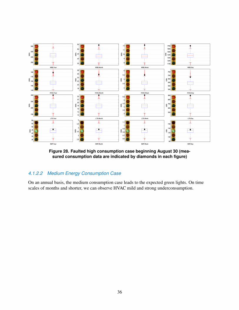
350
400
450
500
WBEYear
MWh
35
40
45
50
55
WBEMonth
MWh
8
9
10
11
12
WBEWeek
MWh
1100
1200
1300
1400
1500
1600
1700
WBEDay
kWh
140
150
160
170
180
HVACYear
MWh
18
20
22
24
26
28
HVACMonth
MWh
4
45
5
55
6
HVACWeek
MWh
500
550
600
650
700
750
HVACDay
kWh
150
200
250
300
LTGYear
MWh
12
14
16
18
20
22
24
LTGMonth
MWh
3
35
4
45
5
55
LTGWeek
MWh
500
600
700
800
900
LTGDay
kWh
30
35
40
45
50
55
60
EQPYear
MWh
25
3
35
4
45
5
EQPMonth
MWh
06
07
08
09
1
11
EQPWeek
MWh
80
100
120
140
160
EQPDay
kWh
Figure 28 Faulted high consumption case beginning August 30 (meashysured consumption data are indicated by diamonds in each figure)
4122 Medium Energy Consumption Case
On an annual basis the medium consumption case leads to the expected green lights On time scales of months and shorter we can observe HVAC mild and strong underconsumption
36
350
400
450
500
WBEYear
MWh
35
40
45
50
55
WBEMonth
MWh
8
9
10
11
12
WBEWeek
MWh
1100
1200
1300
1400
1500
1600
1700
WBEDay
kWh
140
150
160
170
180
HVACYear
MWh
18
20
22
24
26
28
HVACMonth
MWh
4
45
5
55
6
HVACWeek
MWh
500
550
600
650
700
750
HVACDay
kWh
150
200
250
300
LTGYear
MWh
12
14
16
18
20
22
24
LTGMonth
MWh
3
35
4
45
5
55
LTGWeek
MWh
500
600
700
800
900
LTGDay
kWh
30
35
40
45
50
55
60
EQPYear
MWh
25
3
35
4
45
5
EQPMonth
MWh
06
07
08
09
1
11
EQPWeek
MWh
80
100
120
140
160
EQPDay
kWh
Figure 29 Faulted medium consumption case beginning August 30 (measured consumption data are indicated by diamonds in each figure)
4123 Low Energy Consumption Case
The low consumption case at the 5th percentile of the faulted distribution shows a consistent RL light for all end uses and time scales independent of season
37
300
350
400
450
500
WBEYear
MWh
35
40
45
50
55
WBEMonth
MWh
7
8
9
10
11
12
WBEWeek
MWh
1000
1100
1200
1300
1400
1500
1600
1700
WBEDay
kWh
130
140
150
160
170
180
HVACYear
MWh
18
20
22
24
26
28
HVACMonth
MWh
4
45
5
55
6
HVACWeek
MWh
500
550
600
650
700
750
HVACDay
kWh
150
200
250
300
LTGYear
MWh
12
14
16
18
20
22
24
LTGMonth
MWh
3
35
4
45
5
55
LTGWeek
MWh
500
600
700
800
900
LTGDay
kWh
30
35
40
45
50
55
60
EQPYear
MWh
25
3
35
4
45
5
EQPMonth
MWh
06
07
08
09
1
11
EQPWeek
MWh
80
100
120
140
160
EQPDay
kWh
Figure 30 Faulted low consumption case beginning August 30 (meashysured consumption data are indicated by diamonds in each figure)
Finally we present a sample illustration of how such a decision analysis tool would be deployed in the management of distributed commercial buildings Imagine a building operator is responsishyble for the energy-efficient operation of four buildings in a city Building 1 appears to be healthy all end uses show green signals for all four time scales building 2 suffers from overconsumption problems in the HVAC system that manifest themselves in the last day week and month buildshying 3 exhibits underconsumption in LTG especially during the last week which could speak to failed light sources or delamping measures not yet accounted for in the model finally building 4 suffers from multiple symptoms overconsumption in HVAC and EQP and underconsumption in LTG
38
Figure 31 Example of four buildings managed by a building operator
42 Bayesian Parameter Updating Case Studies
Results related to the probabilistic inference and updating of the uncertain model parameters are presented for September 21 at which point measurements over the past 30 days are used to update the five input parameter distributions that are deemed uncertain The high consumption case representing the 95th percentile of the fault-free conditional distributions is used to compute the likelihood functions for HVAC LTG and EQP for each of the nearly 10000 parameter
39
combinations Based on the simplifying assumptions articulated above we can then find the marginal posterior distribution for each selected uncertain parameter Please note that white Gaussian noise with a signal-to-noise ratio of 25 was added to the time series data of the high consumption case to simulate common measurement noise affecting building measurements Recent work by the same authors has shown the Bayesian inference approach to be robust with respect to a wide range of signal-to-noise ratios and noise colors (Pavlak et al 2014)
Table 9 shows the nominal values used to generate the prior input parameter distributions as well as the parameter values associated with the low medium and high cases investigated in this section The latter represent the ground truth values that will be compared to the posterior distributions for each model parameter to determine whether the measured data are used to update our belief of the uncertain parameters in a way that is consistent with the ground truth data
The table shows that several individual parameters appear inconsistent with the case they beshylong to As one example in the low consumption case the DX coil-rated COP is 31 which is below the nominal value One would expect a higher COP to be associated with the low conshysumption case However given the tradeoffs between lighting and equipment power consumption and the efficiency of the cooling equipment the low consumption case at the 5th percentile of 10000 simulation runs was the result of a less efficient RTU with strongly reduced lighting and equipment power densities The median consumption case resulted from a slightly higher lighting power density lower equipment power density lower occupant density and higher RTU COP all relative to the nominal values The high consumption case at the 95th percentile of all cases is characterized by higher lighting equipment and occupancy densities and lower HVAC equipment efficiency In this case of higher consumption the individual parameter values are all consistent with the theme of the case
Later sections discuss that whatever tradeoffs were at play in leading to the low medium and high cases the Bayesian parameter updating process is changing the posterior parameter disshytributions toward the ground truth values that form the basis of the measured (here surrogate) consumption data To that effect each of the following figures 32 to 46 shows the sampled prior distribution of the uncertain parameter as blue bars the sampled posterior distribution as red bars and the ground truth value that formed the basis of the surrogate measured data as a green vertical line
Gas heating efficiency should have no impact on electricity consumption thus increased electricshyity consumption should be independent from gas heating coil efficiency All the figures showing gas heating efficiency distributions illustrate that the gas heating efficiency posterior distribution is being smeared out ie becoming less informative because the evidence used in the likelihood function does not offer any clear clues about how to shape the posterior Although we show the prior and posterior distributions for gas heating efficiency for all three cases the independence of electricity consumption from gas heating efficiency is seen in a widening posterior in each case
40
Table 9 Building Model Truth Parameters
Parameter Nominal Low Medium High Units
Lighting power density 3230 2699 3309 3615 Wm2
Equipment power density 523 492 496 594 Wm2
Occupant density 0141 0149 0137 0151 perm2
DX coil rated COP 320 310 339 294 -Gas heating coil efficiency 80 74 70 77
421 High Energy Consumption Case
Figures 32 through 36 clearly illustrate how the measured data would be harnessed to update our belief about the uncertain parameters Each figure shows the empirical prior distribution as blue bars the empirical posterior distribution is shown as red bars Where the two distributions overlap a darker purple hue appears As stated above in the high energy consumption case all individual building parameter truth values are consistent with the theme of high energy conshysumption Lighting and equipment power density posteriors move to higher values relative to the nominal values that served as the mean of the normal prior distributions and gravitate toward the truth values (green vertical lines) used to generate the surrogate measured data Similarly occupancy densities in people per square meter are also slightly higher and the DX coil-rated COP is significantly lower than the nominal value gravitating toward the truth values Thus the Bayesian inference learns the truth values that form the basis of the measured data
Figure 32 Lighting power density prior (blue) and posterior (red) distributions on
September 21 based on past 30 days of high energy consumption Truth
value is shown as a green vertical line
Figure 33 Equipment power density prior (blue) and posterior (red) distribushytions on September 21 based on past 30 days of high energy consumption Truth value is shown as a green vertical line
41
Figure 34 Occupant density prior (blue) and posterior (red) distributions on
September 21 based on past 30 days of high energy consumption Truth
value is shown as a green vertical line
Figure 35 DX Coil Rated COP prior (blue) and posterior (red) distributions on
September 21 based on past 30 days of high energy consumption Truth
value is shown as a green vertical line
Figure 36 Gas heating coil efficiency prior (blue) and posterior (red) distributions on September 21 based on past 30 days of high energy consumption Truth value is shown as a green vertical line
422 Medium Energy Consumption Case
Figures 37 through 41 show how in the medium consumption case the data reveal the tradeoffs that form the basis of the medium consumption case A slightly higher lighting power density is compensated for by a significantly lower equipment power density because these two have the identical effects of adding convective internal gains to the sensible energy balance paired with slightly higher COPs Occupant density distribution has not materially changed from prior
42
to posterior in the medium consumption case As in the high consumption case the posterior distributions (except for gas heating efficiency as explained above) have moved in the direction of the truth values that form the foundation of the surrogate measured data
Figure 37 Lighting power density prior (blue) and posterior (red) distributions
on September 21 based on past 30 days of medium energy consumption Truth value is shown as a green vertical line
Figure 38 Equipment power density prior (blue) and posterior (red) distributions
on September 21 based on past 30 days of medium energy consumption Truth value is shown as a green vertical line
Figure 39 Occupant density prior (blue) and posterior (red) distributions on
September 21 based on past 30 days of medium energy consumption Truth value is shown as a green vertical line
Figure 40 DX Coil Rated COP prior (blue) and posterior (red) distributions on
September 21 based on past 30 days of medium energy consumption Truth value is shown as a green vertical line
43
Figure 41 Gas heating coil efficiency prior (blue) and posterior (red) distributions on September 21 based on past 30 days of medium
energy consumption Truth value is shown as a green vertical line
423 Low Energy Consumption Case
Figures 42 through 46 again clearly illustrate how the measured data would be harnessed to update our belief about the uncertain parameters In the low consumption case the data suggest significantly lower lighting and equipment power densities although occupant density seems to materially impact the measured data which lead to a virtually unchanged posterior
As shown in Table 9 the truth value of the DX coil-rated COP is slightly lower than the nominal value which is opposite to the theme of lower energy consumption As explained above the slightly inferior COP is more than compensated for by significantly lower lighting and equipment power densities The posterior COP distribution is close2 to the prior but slightly less than it feels like something is missing here suggesting that the Bayesian inference has learned the truth value
As before electricity consumption should not and does not have informative power for gas heating efficiency leaving the posterior smeared out relative to the prior
2A very heuristic visual interpretation of close was used We simply encourage the reader to determine in which direction the posterior distribution mass has been moving to the left to the right or virtually unchanged relative to the prior distribution In particular the point of using such loose language is to avoid comparing the empirical prior and posterior distributions with a more rigorous metric such as the maximum distance of the two cumulative distribution functions as used in the two-sample Kolmogorov-Smirnof test Future work will look into more rigorous metrics to automate the update process The point we wanted to make in this work however is that evidence is collected and used to inform updates of the input parameter distributions
44
Figure 42 Lighting power density prior (blue) and posterior (red) distributions
on September 21 based on past 30 days of low energy consumption Truth value is shown as a green vertical line
Figure 44 Occupant density prior (blue) and posterior (red) distributions on
September 21 based on past 30 days of low energy consumption Truth
value is shown as a green vertical line
Figure 43 Equipment power density prior (blue) and posterior (red) distribushytions on September 21 based on past 30 days of low energy consumption Truth value is shown as a green vertical line
Figure 45 DX Coil Rated COP prior (blue) and posterior (red) distributions
on September 21 based on past 30 days of low energy consumption Truth value is shown as a green vertical line
45
Figure 46 Gas heating coil efficiency prior (blue) and posterior (red) distributions on September 21 based on past 30 days of low
energy consumption Truth value is shown as a green vertical line
46
5 Summary and Conclusions
A prototype energy signal tool was demonstrated for operational whole-building and system-level energy performance assessment The purpose of the tool is to give an assessment that a building operator or other user can quickly comprehend Toward this end the energy signal tool estimates energy use for various end uses from a low-order lumped-parameter model taking into account uncertainty (via a Monte Carlo method) in model parameters and inputs The result of the modelshying phase is a probability distribution over estimated energy use The range of estimated energy use is divided into intervals based on the observed energy use and the probability that energy use is in an interval is computed as the mass of the estimated energy use distribution in that interval An indicator (traffic light color) is chosen to minimize misclassification cost Model parameter distributions are adjusted over time via Bayesian updating
The experimental study investigated whole-building energy signal accuracy in the presence of uncertainty and faults at the submetered level which may lead to tradeoffs at the whole-building level that are not detectable without submetering Submetering of end uses is recommended to avoid confounding underconsumption and overconsumption among various end uses An examshyple of four building energy signal displays is offered to illustrate energy performance features that could be detected by the energy signal tool The Bayesian inference results presented show that observations can be used to periodically update model parameter distributions and that the posterior distributions indeed gravitate toward the ground truth parameter values that formed the basis of the surrogate measured data We presented results for a 30-day learning cycle
Future improvements in the inference process would eliminate the assumptions of temporal independence of subsequent observations of a particular variable and structural independence of multiple observed variables Accounting for covariance among observed variables will help to better attribute observations to individual model parameters
47
Bibliography
Attia S Gratia E Herde AD Hensen JL (2012) ldquoSimulation-based decision support tool for early stages of zero-energy building designrdquo Energy and Buildings 49(0) pp 2 ndash 15
Augenbroe G Castro D Ramkrishnan K (2009) ldquoDecision model for energy performance improvements in existing buildingsrdquo Journal of Engineering Design and Technology 7(1) pp 21 ndash 36
Balcomb J Curtner A (2000) ldquoMulti-criteria decision-making process for buildingsrdquo Energy Conversion Engineering Conference and Exhibit Vol 1 pp 528 ndash 535 Las Vegas NV USA IEEE
Basso N Garavaglia E Sgambi L Imagawa N (2013) Natural hazards vs Decision-making processes in buildings life cycle management New York NY USA CRC Press
Bauermann K Spiecker S Weber C (3 2014) ldquoIndividual decisions and system development Integrating modelling approaches for the heating marketrdquo Applied Energy 116 pp 149ndash158
Booth A Choudhary R Spiegelhalter D (Feb 2012) ldquoHandling uncertainty in housing stock modelsrdquo Building and Environment 48(0) pp 35ndash47
Bracken C Rajagopalan B Prairie J (Mar 2010) ldquoA multisite seasonal ensemble streamflow forecasting techniquerdquo Water Resources Research 46(3) pp 1ndash12 URL httpdoiwileycom1010292009WR007965
Brandemuehl M Shauna G Inger A (1993) ldquoHVAC2 Toolkit Algorithms and Subroutines for Secondary HVAC System Energy Calculationsrdquo ASHRAE Atlanta GA
Braun JE Chaturvedi N (2002) ldquoAn inverse gray-box model for transient building load predictionrdquo HVACampR Research 8(1) pp 73ndash100
Burkhart MC Heo Y Zavala VM (2014) ldquoMeasurement and verification of building systems under uncertain data A Gaussian process modeling approachrdquo Energy and Buildings 75 pp 189 ndash 198
Chaturvedi N Braun J Bernhard R (2000) Analytical Tools for Dynamic Building Conshytrol Implementation of Thermal Storage in Building Mass American Society of Heating Refrigerating and Air-Conditioning Engineers
Choi JH Aziz A Loftness V (2009) ldquoDecision support for improving occupant environmenshytal satisfaction in office buildings The relationship between sub-set of IEQ satisfaction and overall environmental satisfactionrdquo Ninth International Conference of Healthy Buildings p 747 Syracuse NY USA
48
Cipra BA (2000) ldquoThe best of the 20th century Editors name top 10 algorithmsrdquo SIAM news 33(4) pp 1ndash2
Crawley DB Lawrie LK Winkelmann FC Buhl WF Huang YJ Pedersen CO Strand RK Liesen RJ Fisher DE Witte MJ et al (2001) ldquoEnergyPlus creating a new-generation building energy simulation programrdquo Energy and Buildings 33(4) pp 319ndash331
Das S Chew M Poh KL (2010) ldquoMulti-criteria decision analysis in building maintainability using analytical hierarchy processrdquo Construction Management and Economics 28(10) pp 1043 ndash 1056
De Farias C Soares H Pirmez L Delicato F Santos I Carmo LF De Souza J Zomaya A Dohler M (2014) ldquoA control and decision system for smart buildings using wireless sensor and actuator networksrdquo European Transactions on Telecommunications 25(1) pp 120 ndash 135
De Wit S Augenbroe G (2002) ldquoAnalysis of uncertainty in building design evaluations and its implicationsrdquo Energy and Buildings 34(9) pp 951 ndash 958
Deru M Field K Studer D Benne K Griffith B Torcellini P Halverson M Winiarski D Liu B Rosenberg M Huang J Yazdanian M Crawley D (2010) US Department of Energy Commercial Reference Building Models of the National Building Stock Washington DC US Department of Energy Energy Efficiency and Renewable Energy Office of Building Technologies
Diakaki C Grigoroudis E Kabelis N Kolokotsa D Kalaitzakis K Stavrakakis G (2010) ldquoA multi-objective decision model for the improvement of energy efficiency in buildingsrdquo Energy 35(12) pp 5483 ndash 5496
Diakaki C Grigoroudis E Kolokotsa D (2013) ldquoPerformance study of a multi-objective mathematical programming modelling approach for energy decision-making in buildingsrdquo Energy 59 pp 534 ndash 542
Dodier R Kreider J (1999) ldquoWhole Building Energy Diagnosticsrdquo ASHRAE Trans 105(1) pp 579ndash589
Dodier RH Curtiss PS Kreider JF (1998) ldquoSmall-scale on-line diagnostics for an HVAC systemrdquo Transactions-American Society Of Heating Refrigerating And Air Conditioning Engineers 104 pp 530ndash539
DOE U (2010) ldquoEnergyPlus Engineering Referencerdquo The Reference to EnergyPlus Calculashytions URL httpapps1eereenergygovbuildingsenergypluspdfs engineeringreferencepdf
49
Filippoupolitis A Gelenbe E (2009) ldquoA decision support system for disaster management in buildingsrdquo Summer Computer Simulation Conference pp 141 ndash 147 Society for Modeling amp Simulation International
Florita AR Brackney LJ Otanicar TP Robertson J (2013) ldquoClassification of Commercial Building Electrical Demand Profiles for Energy Storage Applicationsrdquo Journal of Solar Energy Engineering 135(3) p 031020
Gulbinas R Jain RK Taylor JE (2014) ldquoBizWatts A modular socio-technical energy management system for empowering commercial building occupants to conserve energyrdquo Applied Energy In-Press
Gultekin P Anumba CJ Leicht RM (2013) ldquoTowards an integrated process model and decision support system for high performance green retrofitsrdquo Architectural Engineering Conference 2013 pp 912 ndash 923 State College PA United states
Heo Y Augenbroe G Choudhary R (2011) ldquoRisk analysis of energy-efficiency projects based on bayesian calibration of building energy modelsrdquo Twelth Conference of International Building Performance Simulation Association pp 2579 ndash 2586 Sydney AUS
Heo Y Zavala VM (2012) ldquoGaussian process modeling for measurement and verification of building energy savingsrdquo Energy and Buildings 53 pp 7 ndash 18
ISO E (2007) ldquo13790 2007rdquo Energy performance of buildings-Calculation of energy use for space heating and cooling
Jaynes ET (2003) Probability theory the logic of science Cambridge university press
Judkoff R Balcomb J Hancock C Barker G Subbarao K (2000) Side-By-Side Thermal Tests of Modular Offices A Validation Study of the STEM Method NREL Report TP-550shy23940 National Renewable Energy Laboratory
Judkoff R Wortman D OrsquoDoherty B Burch J (20081983) Methodology for Validating Building Energy Analysis Simulations NREL Report No TP-550-42059 National Renewable Energy Laboratory Golden CO
Kiluk S (11 2014) ldquoDynamic classification system in large-scale supervision of energy effishyciency in buildingsrdquo Applied Energy 132 pp 1ndash14
Kolokotsa D Diakaki C Grigoroudis E Stavrakakis G Kalaitzakis K (2009) ldquoDecishysion support methodologies on the energy efficiency and energy management in buildingsrdquo Advances in Building Energy Research 3(1) pp 121 ndash 146
Lauret P Miranville F Boyer H Garde F Adelard L (May 2006) ldquoBayesian parameter estimation of convective heat transfer coefficients of a roof-mounted radiant barrier systemrdquo Journal of Solar Energy Engineering 128 pp 213 ndash 225
50
Lee BD Sun Y Augenbroe G Paredis CJ (2013a) ldquoTowards better prediction of building performance A workbench to analyze uncertainty in building simulationrdquo Thirteenth Internashytional Conference of the International Building Performance Simulation Association pp 1231 ndash 1238 Chambery France
Lee SH Augenbroe G Lee JK Zhao F (2013b) ldquoA design methodology for energy infrastructures at the campus scalerdquo Computer-Aided Civil and Infrastructure Engineering 28(10) pp 753 ndash 768
Lee S Liu Y Chunduri S Solnosky RL Messner JI Leicht RM Anumba CJ (2012) ldquoDevelopment of a process model to support integrated design for energy efficient buildingsrdquo International Conference on Computing in Civil Engineering pp 261 ndash 268 Clearwater Beach FL USA
Li Z Heo Y Augenbroe G (2009) ldquoHVAC design informed by organizational simulationrdquo Eleventh International IBPSA Conference pp 2198 ndash 2203 Glasgow UK
Mohseni H Setunge S Zhang GM Wakefield R (2013) ldquoCondition monitoring and condition aggregation for optimised decision making in management of buildingsrdquo Applied Mechanics and Materials 438-439 pp 1719 ndash 1725
Moon HJ Augenbroe G (2008) ldquoEmpowerment of decision-makers in mould remediationrdquo Building Research and Information 36(5) pp 486 ndash 498
Neumann C Jacob D Burhenne S Florita A Burger E Schmidt F (2011) Model-Based Methods for Fault Detection and Optimization in Building Operations (Modellbasierte Methoden fuumlr die Fehlererkennung und Optimierung im Gebaumludebetrieb) Fraunhofer ISE
Pavlak G Florita A Henze G Rajagopalan B (2014) ldquoComparison of Traditional and Bayesian Calibration Techniques for Gray-Box Modelingrdquo Journal of Architectural Engineershying 20(2) p 04013011
Piotr R Laurence B Alison C Ahmed AS (2012) ldquoDecision making aid for selection of renewablesustainable energy systems for buildingsrdquo International Conference on Sustainable Design and Construction pp 306 ndash 313 Kansas City MO USA ASCE
Rafiq M (2000) ldquoImportance of Pareto optimum solutions in making informed decisions in engineering designrdquo Eighth International Conference on Computing in Civil and Building Engineering Vol 2 pp 1325 ndash 1333 Stanford CA USA ASCE
Sanctis GD Fischer K Kohler J Fontana M Faber M (2011) A probabilistic frameshywork for generic fire risk assessment and risk-based decision making in buildings Zurich Switzerland CRC Press
Seem J (1987) Modeling of heat transfer in buildings PhD Thesis University of Wisconsin-Madison
51
Sivia D Skilling J (2006) ldquoParameter estimation IIrdquo Data Analysis A Bayesian Tutorial Chap 3 pp 35 ndash 77 Oxford University Press
Subbarao K (1988a) PSTAR - Primary and Secondary Terms-Analysis and Renormalization A Unified Approach to Building and Energy Simulations and Short-Term Testing A Summary NREL Report TR-254-3347 National Renewable Energy Laboratory
mdashmdashmdash (1988b) PSTAR - Primary and Secondary Terms Analysis and Renormalization A Unified Approach to Building Energy Simulations and Short-Term Monitoring NREL Report TR-254-3175 National Renewable Energy Laboratory
Subbarao K Burch J Hancock C Lekov A Balcomb J (1988) Short-term Energy Monishytoring (STEM) Application of the PSTAR Method to a Residence in Fredericksburg Virginia NREL Report TR-254-3356 National Renewable Energy Laboratory
Subbarao K Mort D Burch J (1985) Short-Term Measurements for the Determination of Envelope Retrofit Performance NREL Report TP-253-2639 National Renewable Energy Laboratory
Sun Y Heo Y Tan M Xie H Jeff Wu C Augenbroe G (2014) ldquoUncertainty quantificashytion of microclimate variables in building energy modelsrdquo Journal of Building Performance Simulation 7(1) pp 17 ndash 32
Takizawa A Kawamura H Tani A (2000) ldquoSimulation of urban system ldquoas it could berdquo by multiagent modelrdquo Eighth International Conference on Computing in Civil and Building Engineering Vol 2 pp 1566 ndash 1573 Stanford CA USA ASCE
Thompson BP Bank LC (2010) ldquoUse of system dynamics as a decision-making tool in building design and operationrdquo Building and Environment 45(4) pp 1006 ndash 1015
Ugwu O Anumba C Newnham L Thorpe A (2000) ldquoAgent-oriented collaborative design of industrial buildingsrdquo Eighth International Conference on Computing in Civil and Building Engineering Vol 1 pp 333 ndash 340 Stanford CA USA ASCE
Vinh A (2009) ldquoComputer-based monitoring for decision support systems and disaster preshyparedness in buildingsrdquo Systemics Cybernetrics and Informatics 7 pp 51ndash56
Wang L Greenberg S Fiegel J Rubalcava A Earni S Pang X Yin R Woodworth S Hernandez-Maldonado J (2 2013) ldquoMonitoring-based HVAC commissioning of an existing office building for energy efficiencyrdquo Applied Energy 102 pp 1382ndash1390
Zeiler W Maaijen R Maassen W (2012) ldquoDecision support for sustainable healthier and more productive buildingsrdquo Tenth International Conference Healthy Buildings pp 1ndash6 Brisbane AUS
52
Zhao P Suryanarayanan S Simoes MG (2010) ldquoAn energy management system for building structures using a multi-agent decision-making control methodologyrdquo Industry Applications Society Annual Meeting pp 1ndash8 Houston TX USA IEEE
Zhao Y Wang S Xiao F (12 2013) ldquoPattern recognition-based chillers fault detection method using Support Vector Data Descriptionrdquo Applied Energy 112 pp 1041ndash1048
53
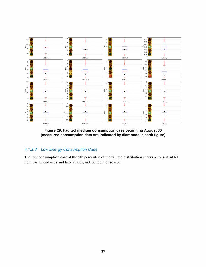
350
400
450
500
WBEYear
MWh
35
40
45
50
55
WBEMonth
MWh
8
9
10
11
12
WBEWeek
MWh
1100
1200
1300
1400
1500
1600
1700
WBEDay
kWh
140
150
160
170
180
HVACYear
MWh
18
20
22
24
26
28
HVACMonth
MWh
4
45
5
55
6
HVACWeek
MWh
500
550
600
650
700
750
HVACDay
kWh
150
200
250
300
LTGYear
MWh
12
14
16
18
20
22
24
LTGMonth
MWh
3
35
4
45
5
55
LTGWeek
MWh
500
600
700
800
900
LTGDay
kWh
30
35
40
45
50
55
60
EQPYear
MWh
25
3
35
4
45
5
EQPMonth
MWh
06
07
08
09
1
11
EQPWeek
MWh
80
100
120
140
160
EQPDay
kWh
Figure 29 Faulted medium consumption case beginning August 30 (measured consumption data are indicated by diamonds in each figure)
4123 Low Energy Consumption Case
The low consumption case at the 5th percentile of the faulted distribution shows a consistent RL light for all end uses and time scales independent of season
37
300
350
400
450
500
WBEYear
MWh
35
40
45
50
55
WBEMonth
MWh
7
8
9
10
11
12
WBEWeek
MWh
1000
1100
1200
1300
1400
1500
1600
1700
WBEDay
kWh
130
140
150
160
170
180
HVACYear
MWh
18
20
22
24
26
28
HVACMonth
MWh
4
45
5
55
6
HVACWeek
MWh
500
550
600
650
700
750
HVACDay
kWh
150
200
250
300
LTGYear
MWh
12
14
16
18
20
22
24
LTGMonth
MWh
3
35
4
45
5
55
LTGWeek
MWh
500
600
700
800
900
LTGDay
kWh
30
35
40
45
50
55
60
EQPYear
MWh
25
3
35
4
45
5
EQPMonth
MWh
06
07
08
09
1
11
EQPWeek
MWh
80
100
120
140
160
EQPDay
kWh
Figure 30 Faulted low consumption case beginning August 30 (meashysured consumption data are indicated by diamonds in each figure)
Finally we present a sample illustration of how such a decision analysis tool would be deployed in the management of distributed commercial buildings Imagine a building operator is responsishyble for the energy-efficient operation of four buildings in a city Building 1 appears to be healthy all end uses show green signals for all four time scales building 2 suffers from overconsumption problems in the HVAC system that manifest themselves in the last day week and month buildshying 3 exhibits underconsumption in LTG especially during the last week which could speak to failed light sources or delamping measures not yet accounted for in the model finally building 4 suffers from multiple symptoms overconsumption in HVAC and EQP and underconsumption in LTG
38
Figure 31 Example of four buildings managed by a building operator
42 Bayesian Parameter Updating Case Studies
Results related to the probabilistic inference and updating of the uncertain model parameters are presented for September 21 at which point measurements over the past 30 days are used to update the five input parameter distributions that are deemed uncertain The high consumption case representing the 95th percentile of the fault-free conditional distributions is used to compute the likelihood functions for HVAC LTG and EQP for each of the nearly 10000 parameter
39
combinations Based on the simplifying assumptions articulated above we can then find the marginal posterior distribution for each selected uncertain parameter Please note that white Gaussian noise with a signal-to-noise ratio of 25 was added to the time series data of the high consumption case to simulate common measurement noise affecting building measurements Recent work by the same authors has shown the Bayesian inference approach to be robust with respect to a wide range of signal-to-noise ratios and noise colors (Pavlak et al 2014)
Table 9 shows the nominal values used to generate the prior input parameter distributions as well as the parameter values associated with the low medium and high cases investigated in this section The latter represent the ground truth values that will be compared to the posterior distributions for each model parameter to determine whether the measured data are used to update our belief of the uncertain parameters in a way that is consistent with the ground truth data
The table shows that several individual parameters appear inconsistent with the case they beshylong to As one example in the low consumption case the DX coil-rated COP is 31 which is below the nominal value One would expect a higher COP to be associated with the low conshysumption case However given the tradeoffs between lighting and equipment power consumption and the efficiency of the cooling equipment the low consumption case at the 5th percentile of 10000 simulation runs was the result of a less efficient RTU with strongly reduced lighting and equipment power densities The median consumption case resulted from a slightly higher lighting power density lower equipment power density lower occupant density and higher RTU COP all relative to the nominal values The high consumption case at the 95th percentile of all cases is characterized by higher lighting equipment and occupancy densities and lower HVAC equipment efficiency In this case of higher consumption the individual parameter values are all consistent with the theme of the case
Later sections discuss that whatever tradeoffs were at play in leading to the low medium and high cases the Bayesian parameter updating process is changing the posterior parameter disshytributions toward the ground truth values that form the basis of the measured (here surrogate) consumption data To that effect each of the following figures 32 to 46 shows the sampled prior distribution of the uncertain parameter as blue bars the sampled posterior distribution as red bars and the ground truth value that formed the basis of the surrogate measured data as a green vertical line
Gas heating efficiency should have no impact on electricity consumption thus increased electricshyity consumption should be independent from gas heating coil efficiency All the figures showing gas heating efficiency distributions illustrate that the gas heating efficiency posterior distribution is being smeared out ie becoming less informative because the evidence used in the likelihood function does not offer any clear clues about how to shape the posterior Although we show the prior and posterior distributions for gas heating efficiency for all three cases the independence of electricity consumption from gas heating efficiency is seen in a widening posterior in each case
40
Table 9 Building Model Truth Parameters
Parameter Nominal Low Medium High Units
Lighting power density 3230 2699 3309 3615 Wm2
Equipment power density 523 492 496 594 Wm2
Occupant density 0141 0149 0137 0151 perm2
DX coil rated COP 320 310 339 294 -Gas heating coil efficiency 80 74 70 77
421 High Energy Consumption Case
Figures 32 through 36 clearly illustrate how the measured data would be harnessed to update our belief about the uncertain parameters Each figure shows the empirical prior distribution as blue bars the empirical posterior distribution is shown as red bars Where the two distributions overlap a darker purple hue appears As stated above in the high energy consumption case all individual building parameter truth values are consistent with the theme of high energy conshysumption Lighting and equipment power density posteriors move to higher values relative to the nominal values that served as the mean of the normal prior distributions and gravitate toward the truth values (green vertical lines) used to generate the surrogate measured data Similarly occupancy densities in people per square meter are also slightly higher and the DX coil-rated COP is significantly lower than the nominal value gravitating toward the truth values Thus the Bayesian inference learns the truth values that form the basis of the measured data
Figure 32 Lighting power density prior (blue) and posterior (red) distributions on
September 21 based on past 30 days of high energy consumption Truth
value is shown as a green vertical line
Figure 33 Equipment power density prior (blue) and posterior (red) distribushytions on September 21 based on past 30 days of high energy consumption Truth value is shown as a green vertical line
41
Figure 34 Occupant density prior (blue) and posterior (red) distributions on
September 21 based on past 30 days of high energy consumption Truth
value is shown as a green vertical line
Figure 35 DX Coil Rated COP prior (blue) and posterior (red) distributions on
September 21 based on past 30 days of high energy consumption Truth
value is shown as a green vertical line
Figure 36 Gas heating coil efficiency prior (blue) and posterior (red) distributions on September 21 based on past 30 days of high energy consumption Truth value is shown as a green vertical line
422 Medium Energy Consumption Case
Figures 37 through 41 show how in the medium consumption case the data reveal the tradeoffs that form the basis of the medium consumption case A slightly higher lighting power density is compensated for by a significantly lower equipment power density because these two have the identical effects of adding convective internal gains to the sensible energy balance paired with slightly higher COPs Occupant density distribution has not materially changed from prior
42
to posterior in the medium consumption case As in the high consumption case the posterior distributions (except for gas heating efficiency as explained above) have moved in the direction of the truth values that form the foundation of the surrogate measured data
Figure 37 Lighting power density prior (blue) and posterior (red) distributions
on September 21 based on past 30 days of medium energy consumption Truth value is shown as a green vertical line
Figure 38 Equipment power density prior (blue) and posterior (red) distributions
on September 21 based on past 30 days of medium energy consumption Truth value is shown as a green vertical line
Figure 39 Occupant density prior (blue) and posterior (red) distributions on
September 21 based on past 30 days of medium energy consumption Truth value is shown as a green vertical line
Figure 40 DX Coil Rated COP prior (blue) and posterior (red) distributions on
September 21 based on past 30 days of medium energy consumption Truth value is shown as a green vertical line
43
Figure 41 Gas heating coil efficiency prior (blue) and posterior (red) distributions on September 21 based on past 30 days of medium
energy consumption Truth value is shown as a green vertical line
423 Low Energy Consumption Case
Figures 42 through 46 again clearly illustrate how the measured data would be harnessed to update our belief about the uncertain parameters In the low consumption case the data suggest significantly lower lighting and equipment power densities although occupant density seems to materially impact the measured data which lead to a virtually unchanged posterior
As shown in Table 9 the truth value of the DX coil-rated COP is slightly lower than the nominal value which is opposite to the theme of lower energy consumption As explained above the slightly inferior COP is more than compensated for by significantly lower lighting and equipment power densities The posterior COP distribution is close2 to the prior but slightly less than it feels like something is missing here suggesting that the Bayesian inference has learned the truth value
As before electricity consumption should not and does not have informative power for gas heating efficiency leaving the posterior smeared out relative to the prior
2A very heuristic visual interpretation of close was used We simply encourage the reader to determine in which direction the posterior distribution mass has been moving to the left to the right or virtually unchanged relative to the prior distribution In particular the point of using such loose language is to avoid comparing the empirical prior and posterior distributions with a more rigorous metric such as the maximum distance of the two cumulative distribution functions as used in the two-sample Kolmogorov-Smirnof test Future work will look into more rigorous metrics to automate the update process The point we wanted to make in this work however is that evidence is collected and used to inform updates of the input parameter distributions
44
Figure 42 Lighting power density prior (blue) and posterior (red) distributions
on September 21 based on past 30 days of low energy consumption Truth value is shown as a green vertical line
Figure 44 Occupant density prior (blue) and posterior (red) distributions on
September 21 based on past 30 days of low energy consumption Truth
value is shown as a green vertical line
Figure 43 Equipment power density prior (blue) and posterior (red) distribushytions on September 21 based on past 30 days of low energy consumption Truth value is shown as a green vertical line
Figure 45 DX Coil Rated COP prior (blue) and posterior (red) distributions
on September 21 based on past 30 days of low energy consumption Truth value is shown as a green vertical line
45
Figure 46 Gas heating coil efficiency prior (blue) and posterior (red) distributions on September 21 based on past 30 days of low
energy consumption Truth value is shown as a green vertical line
46
5 Summary and Conclusions
A prototype energy signal tool was demonstrated for operational whole-building and system-level energy performance assessment The purpose of the tool is to give an assessment that a building operator or other user can quickly comprehend Toward this end the energy signal tool estimates energy use for various end uses from a low-order lumped-parameter model taking into account uncertainty (via a Monte Carlo method) in model parameters and inputs The result of the modelshying phase is a probability distribution over estimated energy use The range of estimated energy use is divided into intervals based on the observed energy use and the probability that energy use is in an interval is computed as the mass of the estimated energy use distribution in that interval An indicator (traffic light color) is chosen to minimize misclassification cost Model parameter distributions are adjusted over time via Bayesian updating
The experimental study investigated whole-building energy signal accuracy in the presence of uncertainty and faults at the submetered level which may lead to tradeoffs at the whole-building level that are not detectable without submetering Submetering of end uses is recommended to avoid confounding underconsumption and overconsumption among various end uses An examshyple of four building energy signal displays is offered to illustrate energy performance features that could be detected by the energy signal tool The Bayesian inference results presented show that observations can be used to periodically update model parameter distributions and that the posterior distributions indeed gravitate toward the ground truth parameter values that formed the basis of the surrogate measured data We presented results for a 30-day learning cycle
Future improvements in the inference process would eliminate the assumptions of temporal independence of subsequent observations of a particular variable and structural independence of multiple observed variables Accounting for covariance among observed variables will help to better attribute observations to individual model parameters
47
Bibliography
Attia S Gratia E Herde AD Hensen JL (2012) ldquoSimulation-based decision support tool for early stages of zero-energy building designrdquo Energy and Buildings 49(0) pp 2 ndash 15
Augenbroe G Castro D Ramkrishnan K (2009) ldquoDecision model for energy performance improvements in existing buildingsrdquo Journal of Engineering Design and Technology 7(1) pp 21 ndash 36
Balcomb J Curtner A (2000) ldquoMulti-criteria decision-making process for buildingsrdquo Energy Conversion Engineering Conference and Exhibit Vol 1 pp 528 ndash 535 Las Vegas NV USA IEEE
Basso N Garavaglia E Sgambi L Imagawa N (2013) Natural hazards vs Decision-making processes in buildings life cycle management New York NY USA CRC Press
Bauermann K Spiecker S Weber C (3 2014) ldquoIndividual decisions and system development Integrating modelling approaches for the heating marketrdquo Applied Energy 116 pp 149ndash158
Booth A Choudhary R Spiegelhalter D (Feb 2012) ldquoHandling uncertainty in housing stock modelsrdquo Building and Environment 48(0) pp 35ndash47
Bracken C Rajagopalan B Prairie J (Mar 2010) ldquoA multisite seasonal ensemble streamflow forecasting techniquerdquo Water Resources Research 46(3) pp 1ndash12 URL httpdoiwileycom1010292009WR007965
Brandemuehl M Shauna G Inger A (1993) ldquoHVAC2 Toolkit Algorithms and Subroutines for Secondary HVAC System Energy Calculationsrdquo ASHRAE Atlanta GA
Braun JE Chaturvedi N (2002) ldquoAn inverse gray-box model for transient building load predictionrdquo HVACampR Research 8(1) pp 73ndash100
Burkhart MC Heo Y Zavala VM (2014) ldquoMeasurement and verification of building systems under uncertain data A Gaussian process modeling approachrdquo Energy and Buildings 75 pp 189 ndash 198
Chaturvedi N Braun J Bernhard R (2000) Analytical Tools for Dynamic Building Conshytrol Implementation of Thermal Storage in Building Mass American Society of Heating Refrigerating and Air-Conditioning Engineers
Choi JH Aziz A Loftness V (2009) ldquoDecision support for improving occupant environmenshytal satisfaction in office buildings The relationship between sub-set of IEQ satisfaction and overall environmental satisfactionrdquo Ninth International Conference of Healthy Buildings p 747 Syracuse NY USA
48
Cipra BA (2000) ldquoThe best of the 20th century Editors name top 10 algorithmsrdquo SIAM news 33(4) pp 1ndash2
Crawley DB Lawrie LK Winkelmann FC Buhl WF Huang YJ Pedersen CO Strand RK Liesen RJ Fisher DE Witte MJ et al (2001) ldquoEnergyPlus creating a new-generation building energy simulation programrdquo Energy and Buildings 33(4) pp 319ndash331
Das S Chew M Poh KL (2010) ldquoMulti-criteria decision analysis in building maintainability using analytical hierarchy processrdquo Construction Management and Economics 28(10) pp 1043 ndash 1056
De Farias C Soares H Pirmez L Delicato F Santos I Carmo LF De Souza J Zomaya A Dohler M (2014) ldquoA control and decision system for smart buildings using wireless sensor and actuator networksrdquo European Transactions on Telecommunications 25(1) pp 120 ndash 135
De Wit S Augenbroe G (2002) ldquoAnalysis of uncertainty in building design evaluations and its implicationsrdquo Energy and Buildings 34(9) pp 951 ndash 958
Deru M Field K Studer D Benne K Griffith B Torcellini P Halverson M Winiarski D Liu B Rosenberg M Huang J Yazdanian M Crawley D (2010) US Department of Energy Commercial Reference Building Models of the National Building Stock Washington DC US Department of Energy Energy Efficiency and Renewable Energy Office of Building Technologies
Diakaki C Grigoroudis E Kabelis N Kolokotsa D Kalaitzakis K Stavrakakis G (2010) ldquoA multi-objective decision model for the improvement of energy efficiency in buildingsrdquo Energy 35(12) pp 5483 ndash 5496
Diakaki C Grigoroudis E Kolokotsa D (2013) ldquoPerformance study of a multi-objective mathematical programming modelling approach for energy decision-making in buildingsrdquo Energy 59 pp 534 ndash 542
Dodier R Kreider J (1999) ldquoWhole Building Energy Diagnosticsrdquo ASHRAE Trans 105(1) pp 579ndash589
Dodier RH Curtiss PS Kreider JF (1998) ldquoSmall-scale on-line diagnostics for an HVAC systemrdquo Transactions-American Society Of Heating Refrigerating And Air Conditioning Engineers 104 pp 530ndash539
DOE U (2010) ldquoEnergyPlus Engineering Referencerdquo The Reference to EnergyPlus Calculashytions URL httpapps1eereenergygovbuildingsenergypluspdfs engineeringreferencepdf
49
Filippoupolitis A Gelenbe E (2009) ldquoA decision support system for disaster management in buildingsrdquo Summer Computer Simulation Conference pp 141 ndash 147 Society for Modeling amp Simulation International
Florita AR Brackney LJ Otanicar TP Robertson J (2013) ldquoClassification of Commercial Building Electrical Demand Profiles for Energy Storage Applicationsrdquo Journal of Solar Energy Engineering 135(3) p 031020
Gulbinas R Jain RK Taylor JE (2014) ldquoBizWatts A modular socio-technical energy management system for empowering commercial building occupants to conserve energyrdquo Applied Energy In-Press
Gultekin P Anumba CJ Leicht RM (2013) ldquoTowards an integrated process model and decision support system for high performance green retrofitsrdquo Architectural Engineering Conference 2013 pp 912 ndash 923 State College PA United states
Heo Y Augenbroe G Choudhary R (2011) ldquoRisk analysis of energy-efficiency projects based on bayesian calibration of building energy modelsrdquo Twelth Conference of International Building Performance Simulation Association pp 2579 ndash 2586 Sydney AUS
Heo Y Zavala VM (2012) ldquoGaussian process modeling for measurement and verification of building energy savingsrdquo Energy and Buildings 53 pp 7 ndash 18
ISO E (2007) ldquo13790 2007rdquo Energy performance of buildings-Calculation of energy use for space heating and cooling
Jaynes ET (2003) Probability theory the logic of science Cambridge university press
Judkoff R Balcomb J Hancock C Barker G Subbarao K (2000) Side-By-Side Thermal Tests of Modular Offices A Validation Study of the STEM Method NREL Report TP-550shy23940 National Renewable Energy Laboratory
Judkoff R Wortman D OrsquoDoherty B Burch J (20081983) Methodology for Validating Building Energy Analysis Simulations NREL Report No TP-550-42059 National Renewable Energy Laboratory Golden CO
Kiluk S (11 2014) ldquoDynamic classification system in large-scale supervision of energy effishyciency in buildingsrdquo Applied Energy 132 pp 1ndash14
Kolokotsa D Diakaki C Grigoroudis E Stavrakakis G Kalaitzakis K (2009) ldquoDecishysion support methodologies on the energy efficiency and energy management in buildingsrdquo Advances in Building Energy Research 3(1) pp 121 ndash 146
Lauret P Miranville F Boyer H Garde F Adelard L (May 2006) ldquoBayesian parameter estimation of convective heat transfer coefficients of a roof-mounted radiant barrier systemrdquo Journal of Solar Energy Engineering 128 pp 213 ndash 225
50
Lee BD Sun Y Augenbroe G Paredis CJ (2013a) ldquoTowards better prediction of building performance A workbench to analyze uncertainty in building simulationrdquo Thirteenth Internashytional Conference of the International Building Performance Simulation Association pp 1231 ndash 1238 Chambery France
Lee SH Augenbroe G Lee JK Zhao F (2013b) ldquoA design methodology for energy infrastructures at the campus scalerdquo Computer-Aided Civil and Infrastructure Engineering 28(10) pp 753 ndash 768
Lee S Liu Y Chunduri S Solnosky RL Messner JI Leicht RM Anumba CJ (2012) ldquoDevelopment of a process model to support integrated design for energy efficient buildingsrdquo International Conference on Computing in Civil Engineering pp 261 ndash 268 Clearwater Beach FL USA
Li Z Heo Y Augenbroe G (2009) ldquoHVAC design informed by organizational simulationrdquo Eleventh International IBPSA Conference pp 2198 ndash 2203 Glasgow UK
Mohseni H Setunge S Zhang GM Wakefield R (2013) ldquoCondition monitoring and condition aggregation for optimised decision making in management of buildingsrdquo Applied Mechanics and Materials 438-439 pp 1719 ndash 1725
Moon HJ Augenbroe G (2008) ldquoEmpowerment of decision-makers in mould remediationrdquo Building Research and Information 36(5) pp 486 ndash 498
Neumann C Jacob D Burhenne S Florita A Burger E Schmidt F (2011) Model-Based Methods for Fault Detection and Optimization in Building Operations (Modellbasierte Methoden fuumlr die Fehlererkennung und Optimierung im Gebaumludebetrieb) Fraunhofer ISE
Pavlak G Florita A Henze G Rajagopalan B (2014) ldquoComparison of Traditional and Bayesian Calibration Techniques for Gray-Box Modelingrdquo Journal of Architectural Engineershying 20(2) p 04013011
Piotr R Laurence B Alison C Ahmed AS (2012) ldquoDecision making aid for selection of renewablesustainable energy systems for buildingsrdquo International Conference on Sustainable Design and Construction pp 306 ndash 313 Kansas City MO USA ASCE
Rafiq M (2000) ldquoImportance of Pareto optimum solutions in making informed decisions in engineering designrdquo Eighth International Conference on Computing in Civil and Building Engineering Vol 2 pp 1325 ndash 1333 Stanford CA USA ASCE
Sanctis GD Fischer K Kohler J Fontana M Faber M (2011) A probabilistic frameshywork for generic fire risk assessment and risk-based decision making in buildings Zurich Switzerland CRC Press
Seem J (1987) Modeling of heat transfer in buildings PhD Thesis University of Wisconsin-Madison
51
Sivia D Skilling J (2006) ldquoParameter estimation IIrdquo Data Analysis A Bayesian Tutorial Chap 3 pp 35 ndash 77 Oxford University Press
Subbarao K (1988a) PSTAR - Primary and Secondary Terms-Analysis and Renormalization A Unified Approach to Building and Energy Simulations and Short-Term Testing A Summary NREL Report TR-254-3347 National Renewable Energy Laboratory
mdashmdashmdash (1988b) PSTAR - Primary and Secondary Terms Analysis and Renormalization A Unified Approach to Building Energy Simulations and Short-Term Monitoring NREL Report TR-254-3175 National Renewable Energy Laboratory
Subbarao K Burch J Hancock C Lekov A Balcomb J (1988) Short-term Energy Monishytoring (STEM) Application of the PSTAR Method to a Residence in Fredericksburg Virginia NREL Report TR-254-3356 National Renewable Energy Laboratory
Subbarao K Mort D Burch J (1985) Short-Term Measurements for the Determination of Envelope Retrofit Performance NREL Report TP-253-2639 National Renewable Energy Laboratory
Sun Y Heo Y Tan M Xie H Jeff Wu C Augenbroe G (2014) ldquoUncertainty quantificashytion of microclimate variables in building energy modelsrdquo Journal of Building Performance Simulation 7(1) pp 17 ndash 32
Takizawa A Kawamura H Tani A (2000) ldquoSimulation of urban system ldquoas it could berdquo by multiagent modelrdquo Eighth International Conference on Computing in Civil and Building Engineering Vol 2 pp 1566 ndash 1573 Stanford CA USA ASCE
Thompson BP Bank LC (2010) ldquoUse of system dynamics as a decision-making tool in building design and operationrdquo Building and Environment 45(4) pp 1006 ndash 1015
Ugwu O Anumba C Newnham L Thorpe A (2000) ldquoAgent-oriented collaborative design of industrial buildingsrdquo Eighth International Conference on Computing in Civil and Building Engineering Vol 1 pp 333 ndash 340 Stanford CA USA ASCE
Vinh A (2009) ldquoComputer-based monitoring for decision support systems and disaster preshyparedness in buildingsrdquo Systemics Cybernetrics and Informatics 7 pp 51ndash56
Wang L Greenberg S Fiegel J Rubalcava A Earni S Pang X Yin R Woodworth S Hernandez-Maldonado J (2 2013) ldquoMonitoring-based HVAC commissioning of an existing office building for energy efficiencyrdquo Applied Energy 102 pp 1382ndash1390
Zeiler W Maaijen R Maassen W (2012) ldquoDecision support for sustainable healthier and more productive buildingsrdquo Tenth International Conference Healthy Buildings pp 1ndash6 Brisbane AUS
52
Zhao P Suryanarayanan S Simoes MG (2010) ldquoAn energy management system for building structures using a multi-agent decision-making control methodologyrdquo Industry Applications Society Annual Meeting pp 1ndash8 Houston TX USA IEEE
Zhao Y Wang S Xiao F (12 2013) ldquoPattern recognition-based chillers fault detection method using Support Vector Data Descriptionrdquo Applied Energy 112 pp 1041ndash1048
53
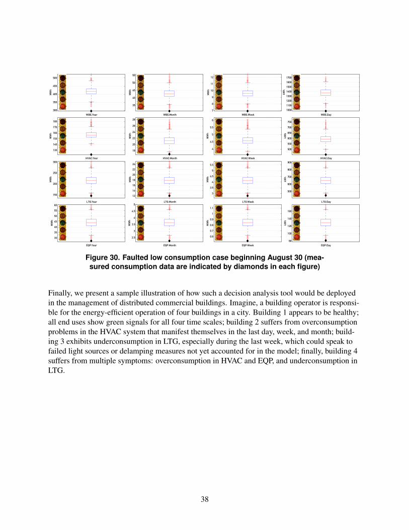
300
350
400
450
500
WBEYear
MWh
35
40
45
50
55
WBEMonth
MWh
7
8
9
10
11
12
WBEWeek
MWh
1000
1100
1200
1300
1400
1500
1600
1700
WBEDay
kWh
130
140
150
160
170
180
HVACYear
MWh
18
20
22
24
26
28
HVACMonth
MWh
4
45
5
55
6
HVACWeek
MWh
500
550
600
650
700
750
HVACDay
kWh
150
200
250
300
LTGYear
MWh
12
14
16
18
20
22
24
LTGMonth
MWh
3
35
4
45
5
55
LTGWeek
MWh
500
600
700
800
900
LTGDay
kWh
30
35
40
45
50
55
60
EQPYear
MWh
25
3
35
4
45
5
EQPMonth
MWh
06
07
08
09
1
11
EQPWeek
MWh
80
100
120
140
160
EQPDay
kWh
Figure 30 Faulted low consumption case beginning August 30 (meashysured consumption data are indicated by diamonds in each figure)
Finally we present a sample illustration of how such a decision analysis tool would be deployed in the management of distributed commercial buildings Imagine a building operator is responsishyble for the energy-efficient operation of four buildings in a city Building 1 appears to be healthy all end uses show green signals for all four time scales building 2 suffers from overconsumption problems in the HVAC system that manifest themselves in the last day week and month buildshying 3 exhibits underconsumption in LTG especially during the last week which could speak to failed light sources or delamping measures not yet accounted for in the model finally building 4 suffers from multiple symptoms overconsumption in HVAC and EQP and underconsumption in LTG
38
Figure 31 Example of four buildings managed by a building operator
42 Bayesian Parameter Updating Case Studies
Results related to the probabilistic inference and updating of the uncertain model parameters are presented for September 21 at which point measurements over the past 30 days are used to update the five input parameter distributions that are deemed uncertain The high consumption case representing the 95th percentile of the fault-free conditional distributions is used to compute the likelihood functions for HVAC LTG and EQP for each of the nearly 10000 parameter
39
combinations Based on the simplifying assumptions articulated above we can then find the marginal posterior distribution for each selected uncertain parameter Please note that white Gaussian noise with a signal-to-noise ratio of 25 was added to the time series data of the high consumption case to simulate common measurement noise affecting building measurements Recent work by the same authors has shown the Bayesian inference approach to be robust with respect to a wide range of signal-to-noise ratios and noise colors (Pavlak et al 2014)
Table 9 shows the nominal values used to generate the prior input parameter distributions as well as the parameter values associated with the low medium and high cases investigated in this section The latter represent the ground truth values that will be compared to the posterior distributions for each model parameter to determine whether the measured data are used to update our belief of the uncertain parameters in a way that is consistent with the ground truth data
The table shows that several individual parameters appear inconsistent with the case they beshylong to As one example in the low consumption case the DX coil-rated COP is 31 which is below the nominal value One would expect a higher COP to be associated with the low conshysumption case However given the tradeoffs between lighting and equipment power consumption and the efficiency of the cooling equipment the low consumption case at the 5th percentile of 10000 simulation runs was the result of a less efficient RTU with strongly reduced lighting and equipment power densities The median consumption case resulted from a slightly higher lighting power density lower equipment power density lower occupant density and higher RTU COP all relative to the nominal values The high consumption case at the 95th percentile of all cases is characterized by higher lighting equipment and occupancy densities and lower HVAC equipment efficiency In this case of higher consumption the individual parameter values are all consistent with the theme of the case
Later sections discuss that whatever tradeoffs were at play in leading to the low medium and high cases the Bayesian parameter updating process is changing the posterior parameter disshytributions toward the ground truth values that form the basis of the measured (here surrogate) consumption data To that effect each of the following figures 32 to 46 shows the sampled prior distribution of the uncertain parameter as blue bars the sampled posterior distribution as red bars and the ground truth value that formed the basis of the surrogate measured data as a green vertical line
Gas heating efficiency should have no impact on electricity consumption thus increased electricshyity consumption should be independent from gas heating coil efficiency All the figures showing gas heating efficiency distributions illustrate that the gas heating efficiency posterior distribution is being smeared out ie becoming less informative because the evidence used in the likelihood function does not offer any clear clues about how to shape the posterior Although we show the prior and posterior distributions for gas heating efficiency for all three cases the independence of electricity consumption from gas heating efficiency is seen in a widening posterior in each case
40
Table 9 Building Model Truth Parameters
Parameter Nominal Low Medium High Units
Lighting power density 3230 2699 3309 3615 Wm2
Equipment power density 523 492 496 594 Wm2
Occupant density 0141 0149 0137 0151 perm2
DX coil rated COP 320 310 339 294 -Gas heating coil efficiency 80 74 70 77
421 High Energy Consumption Case
Figures 32 through 36 clearly illustrate how the measured data would be harnessed to update our belief about the uncertain parameters Each figure shows the empirical prior distribution as blue bars the empirical posterior distribution is shown as red bars Where the two distributions overlap a darker purple hue appears As stated above in the high energy consumption case all individual building parameter truth values are consistent with the theme of high energy conshysumption Lighting and equipment power density posteriors move to higher values relative to the nominal values that served as the mean of the normal prior distributions and gravitate toward the truth values (green vertical lines) used to generate the surrogate measured data Similarly occupancy densities in people per square meter are also slightly higher and the DX coil-rated COP is significantly lower than the nominal value gravitating toward the truth values Thus the Bayesian inference learns the truth values that form the basis of the measured data
Figure 32 Lighting power density prior (blue) and posterior (red) distributions on
September 21 based on past 30 days of high energy consumption Truth
value is shown as a green vertical line
Figure 33 Equipment power density prior (blue) and posterior (red) distribushytions on September 21 based on past 30 days of high energy consumption Truth value is shown as a green vertical line
41
Figure 34 Occupant density prior (blue) and posterior (red) distributions on
September 21 based on past 30 days of high energy consumption Truth
value is shown as a green vertical line
Figure 35 DX Coil Rated COP prior (blue) and posterior (red) distributions on
September 21 based on past 30 days of high energy consumption Truth
value is shown as a green vertical line
Figure 36 Gas heating coil efficiency prior (blue) and posterior (red) distributions on September 21 based on past 30 days of high energy consumption Truth value is shown as a green vertical line
422 Medium Energy Consumption Case
Figures 37 through 41 show how in the medium consumption case the data reveal the tradeoffs that form the basis of the medium consumption case A slightly higher lighting power density is compensated for by a significantly lower equipment power density because these two have the identical effects of adding convective internal gains to the sensible energy balance paired with slightly higher COPs Occupant density distribution has not materially changed from prior
42
to posterior in the medium consumption case As in the high consumption case the posterior distributions (except for gas heating efficiency as explained above) have moved in the direction of the truth values that form the foundation of the surrogate measured data
Figure 37 Lighting power density prior (blue) and posterior (red) distributions
on September 21 based on past 30 days of medium energy consumption Truth value is shown as a green vertical line
Figure 38 Equipment power density prior (blue) and posterior (red) distributions
on September 21 based on past 30 days of medium energy consumption Truth value is shown as a green vertical line
Figure 39 Occupant density prior (blue) and posterior (red) distributions on
September 21 based on past 30 days of medium energy consumption Truth value is shown as a green vertical line
Figure 40 DX Coil Rated COP prior (blue) and posterior (red) distributions on
September 21 based on past 30 days of medium energy consumption Truth value is shown as a green vertical line
43
Figure 41 Gas heating coil efficiency prior (blue) and posterior (red) distributions on September 21 based on past 30 days of medium
energy consumption Truth value is shown as a green vertical line
423 Low Energy Consumption Case
Figures 42 through 46 again clearly illustrate how the measured data would be harnessed to update our belief about the uncertain parameters In the low consumption case the data suggest significantly lower lighting and equipment power densities although occupant density seems to materially impact the measured data which lead to a virtually unchanged posterior
As shown in Table 9 the truth value of the DX coil-rated COP is slightly lower than the nominal value which is opposite to the theme of lower energy consumption As explained above the slightly inferior COP is more than compensated for by significantly lower lighting and equipment power densities The posterior COP distribution is close2 to the prior but slightly less than it feels like something is missing here suggesting that the Bayesian inference has learned the truth value
As before electricity consumption should not and does not have informative power for gas heating efficiency leaving the posterior smeared out relative to the prior
2A very heuristic visual interpretation of close was used We simply encourage the reader to determine in which direction the posterior distribution mass has been moving to the left to the right or virtually unchanged relative to the prior distribution In particular the point of using such loose language is to avoid comparing the empirical prior and posterior distributions with a more rigorous metric such as the maximum distance of the two cumulative distribution functions as used in the two-sample Kolmogorov-Smirnof test Future work will look into more rigorous metrics to automate the update process The point we wanted to make in this work however is that evidence is collected and used to inform updates of the input parameter distributions
44
Figure 42 Lighting power density prior (blue) and posterior (red) distributions
on September 21 based on past 30 days of low energy consumption Truth value is shown as a green vertical line
Figure 44 Occupant density prior (blue) and posterior (red) distributions on
September 21 based on past 30 days of low energy consumption Truth
value is shown as a green vertical line
Figure 43 Equipment power density prior (blue) and posterior (red) distribushytions on September 21 based on past 30 days of low energy consumption Truth value is shown as a green vertical line
Figure 45 DX Coil Rated COP prior (blue) and posterior (red) distributions
on September 21 based on past 30 days of low energy consumption Truth value is shown as a green vertical line
45
Figure 46 Gas heating coil efficiency prior (blue) and posterior (red) distributions on September 21 based on past 30 days of low
energy consumption Truth value is shown as a green vertical line
46
5 Summary and Conclusions
A prototype energy signal tool was demonstrated for operational whole-building and system-level energy performance assessment The purpose of the tool is to give an assessment that a building operator or other user can quickly comprehend Toward this end the energy signal tool estimates energy use for various end uses from a low-order lumped-parameter model taking into account uncertainty (via a Monte Carlo method) in model parameters and inputs The result of the modelshying phase is a probability distribution over estimated energy use The range of estimated energy use is divided into intervals based on the observed energy use and the probability that energy use is in an interval is computed as the mass of the estimated energy use distribution in that interval An indicator (traffic light color) is chosen to minimize misclassification cost Model parameter distributions are adjusted over time via Bayesian updating
The experimental study investigated whole-building energy signal accuracy in the presence of uncertainty and faults at the submetered level which may lead to tradeoffs at the whole-building level that are not detectable without submetering Submetering of end uses is recommended to avoid confounding underconsumption and overconsumption among various end uses An examshyple of four building energy signal displays is offered to illustrate energy performance features that could be detected by the energy signal tool The Bayesian inference results presented show that observations can be used to periodically update model parameter distributions and that the posterior distributions indeed gravitate toward the ground truth parameter values that formed the basis of the surrogate measured data We presented results for a 30-day learning cycle
Future improvements in the inference process would eliminate the assumptions of temporal independence of subsequent observations of a particular variable and structural independence of multiple observed variables Accounting for covariance among observed variables will help to better attribute observations to individual model parameters
47
Bibliography
Attia S Gratia E Herde AD Hensen JL (2012) ldquoSimulation-based decision support tool for early stages of zero-energy building designrdquo Energy and Buildings 49(0) pp 2 ndash 15
Augenbroe G Castro D Ramkrishnan K (2009) ldquoDecision model for energy performance improvements in existing buildingsrdquo Journal of Engineering Design and Technology 7(1) pp 21 ndash 36
Balcomb J Curtner A (2000) ldquoMulti-criteria decision-making process for buildingsrdquo Energy Conversion Engineering Conference and Exhibit Vol 1 pp 528 ndash 535 Las Vegas NV USA IEEE
Basso N Garavaglia E Sgambi L Imagawa N (2013) Natural hazards vs Decision-making processes in buildings life cycle management New York NY USA CRC Press
Bauermann K Spiecker S Weber C (3 2014) ldquoIndividual decisions and system development Integrating modelling approaches for the heating marketrdquo Applied Energy 116 pp 149ndash158
Booth A Choudhary R Spiegelhalter D (Feb 2012) ldquoHandling uncertainty in housing stock modelsrdquo Building and Environment 48(0) pp 35ndash47
Bracken C Rajagopalan B Prairie J (Mar 2010) ldquoA multisite seasonal ensemble streamflow forecasting techniquerdquo Water Resources Research 46(3) pp 1ndash12 URL httpdoiwileycom1010292009WR007965
Brandemuehl M Shauna G Inger A (1993) ldquoHVAC2 Toolkit Algorithms and Subroutines for Secondary HVAC System Energy Calculationsrdquo ASHRAE Atlanta GA
Braun JE Chaturvedi N (2002) ldquoAn inverse gray-box model for transient building load predictionrdquo HVACampR Research 8(1) pp 73ndash100
Burkhart MC Heo Y Zavala VM (2014) ldquoMeasurement and verification of building systems under uncertain data A Gaussian process modeling approachrdquo Energy and Buildings 75 pp 189 ndash 198
Chaturvedi N Braun J Bernhard R (2000) Analytical Tools for Dynamic Building Conshytrol Implementation of Thermal Storage in Building Mass American Society of Heating Refrigerating and Air-Conditioning Engineers
Choi JH Aziz A Loftness V (2009) ldquoDecision support for improving occupant environmenshytal satisfaction in office buildings The relationship between sub-set of IEQ satisfaction and overall environmental satisfactionrdquo Ninth International Conference of Healthy Buildings p 747 Syracuse NY USA
48
Cipra BA (2000) ldquoThe best of the 20th century Editors name top 10 algorithmsrdquo SIAM news 33(4) pp 1ndash2
Crawley DB Lawrie LK Winkelmann FC Buhl WF Huang YJ Pedersen CO Strand RK Liesen RJ Fisher DE Witte MJ et al (2001) ldquoEnergyPlus creating a new-generation building energy simulation programrdquo Energy and Buildings 33(4) pp 319ndash331
Das S Chew M Poh KL (2010) ldquoMulti-criteria decision analysis in building maintainability using analytical hierarchy processrdquo Construction Management and Economics 28(10) pp 1043 ndash 1056
De Farias C Soares H Pirmez L Delicato F Santos I Carmo LF De Souza J Zomaya A Dohler M (2014) ldquoA control and decision system for smart buildings using wireless sensor and actuator networksrdquo European Transactions on Telecommunications 25(1) pp 120 ndash 135
De Wit S Augenbroe G (2002) ldquoAnalysis of uncertainty in building design evaluations and its implicationsrdquo Energy and Buildings 34(9) pp 951 ndash 958
Deru M Field K Studer D Benne K Griffith B Torcellini P Halverson M Winiarski D Liu B Rosenberg M Huang J Yazdanian M Crawley D (2010) US Department of Energy Commercial Reference Building Models of the National Building Stock Washington DC US Department of Energy Energy Efficiency and Renewable Energy Office of Building Technologies
Diakaki C Grigoroudis E Kabelis N Kolokotsa D Kalaitzakis K Stavrakakis G (2010) ldquoA multi-objective decision model for the improvement of energy efficiency in buildingsrdquo Energy 35(12) pp 5483 ndash 5496
Diakaki C Grigoroudis E Kolokotsa D (2013) ldquoPerformance study of a multi-objective mathematical programming modelling approach for energy decision-making in buildingsrdquo Energy 59 pp 534 ndash 542
Dodier R Kreider J (1999) ldquoWhole Building Energy Diagnosticsrdquo ASHRAE Trans 105(1) pp 579ndash589
Dodier RH Curtiss PS Kreider JF (1998) ldquoSmall-scale on-line diagnostics for an HVAC systemrdquo Transactions-American Society Of Heating Refrigerating And Air Conditioning Engineers 104 pp 530ndash539
DOE U (2010) ldquoEnergyPlus Engineering Referencerdquo The Reference to EnergyPlus Calculashytions URL httpapps1eereenergygovbuildingsenergypluspdfs engineeringreferencepdf
49
Filippoupolitis A Gelenbe E (2009) ldquoA decision support system for disaster management in buildingsrdquo Summer Computer Simulation Conference pp 141 ndash 147 Society for Modeling amp Simulation International
Florita AR Brackney LJ Otanicar TP Robertson J (2013) ldquoClassification of Commercial Building Electrical Demand Profiles for Energy Storage Applicationsrdquo Journal of Solar Energy Engineering 135(3) p 031020
Gulbinas R Jain RK Taylor JE (2014) ldquoBizWatts A modular socio-technical energy management system for empowering commercial building occupants to conserve energyrdquo Applied Energy In-Press
Gultekin P Anumba CJ Leicht RM (2013) ldquoTowards an integrated process model and decision support system for high performance green retrofitsrdquo Architectural Engineering Conference 2013 pp 912 ndash 923 State College PA United states
Heo Y Augenbroe G Choudhary R (2011) ldquoRisk analysis of energy-efficiency projects based on bayesian calibration of building energy modelsrdquo Twelth Conference of International Building Performance Simulation Association pp 2579 ndash 2586 Sydney AUS
Heo Y Zavala VM (2012) ldquoGaussian process modeling for measurement and verification of building energy savingsrdquo Energy and Buildings 53 pp 7 ndash 18
ISO E (2007) ldquo13790 2007rdquo Energy performance of buildings-Calculation of energy use for space heating and cooling
Jaynes ET (2003) Probability theory the logic of science Cambridge university press
Judkoff R Balcomb J Hancock C Barker G Subbarao K (2000) Side-By-Side Thermal Tests of Modular Offices A Validation Study of the STEM Method NREL Report TP-550shy23940 National Renewable Energy Laboratory
Judkoff R Wortman D OrsquoDoherty B Burch J (20081983) Methodology for Validating Building Energy Analysis Simulations NREL Report No TP-550-42059 National Renewable Energy Laboratory Golden CO
Kiluk S (11 2014) ldquoDynamic classification system in large-scale supervision of energy effishyciency in buildingsrdquo Applied Energy 132 pp 1ndash14
Kolokotsa D Diakaki C Grigoroudis E Stavrakakis G Kalaitzakis K (2009) ldquoDecishysion support methodologies on the energy efficiency and energy management in buildingsrdquo Advances in Building Energy Research 3(1) pp 121 ndash 146
Lauret P Miranville F Boyer H Garde F Adelard L (May 2006) ldquoBayesian parameter estimation of convective heat transfer coefficients of a roof-mounted radiant barrier systemrdquo Journal of Solar Energy Engineering 128 pp 213 ndash 225
50
Lee BD Sun Y Augenbroe G Paredis CJ (2013a) ldquoTowards better prediction of building performance A workbench to analyze uncertainty in building simulationrdquo Thirteenth Internashytional Conference of the International Building Performance Simulation Association pp 1231 ndash 1238 Chambery France
Lee SH Augenbroe G Lee JK Zhao F (2013b) ldquoA design methodology for energy infrastructures at the campus scalerdquo Computer-Aided Civil and Infrastructure Engineering 28(10) pp 753 ndash 768
Lee S Liu Y Chunduri S Solnosky RL Messner JI Leicht RM Anumba CJ (2012) ldquoDevelopment of a process model to support integrated design for energy efficient buildingsrdquo International Conference on Computing in Civil Engineering pp 261 ndash 268 Clearwater Beach FL USA
Li Z Heo Y Augenbroe G (2009) ldquoHVAC design informed by organizational simulationrdquo Eleventh International IBPSA Conference pp 2198 ndash 2203 Glasgow UK
Mohseni H Setunge S Zhang GM Wakefield R (2013) ldquoCondition monitoring and condition aggregation for optimised decision making in management of buildingsrdquo Applied Mechanics and Materials 438-439 pp 1719 ndash 1725
Moon HJ Augenbroe G (2008) ldquoEmpowerment of decision-makers in mould remediationrdquo Building Research and Information 36(5) pp 486 ndash 498
Neumann C Jacob D Burhenne S Florita A Burger E Schmidt F (2011) Model-Based Methods for Fault Detection and Optimization in Building Operations (Modellbasierte Methoden fuumlr die Fehlererkennung und Optimierung im Gebaumludebetrieb) Fraunhofer ISE
Pavlak G Florita A Henze G Rajagopalan B (2014) ldquoComparison of Traditional and Bayesian Calibration Techniques for Gray-Box Modelingrdquo Journal of Architectural Engineershying 20(2) p 04013011
Piotr R Laurence B Alison C Ahmed AS (2012) ldquoDecision making aid for selection of renewablesustainable energy systems for buildingsrdquo International Conference on Sustainable Design and Construction pp 306 ndash 313 Kansas City MO USA ASCE
Rafiq M (2000) ldquoImportance of Pareto optimum solutions in making informed decisions in engineering designrdquo Eighth International Conference on Computing in Civil and Building Engineering Vol 2 pp 1325 ndash 1333 Stanford CA USA ASCE
Sanctis GD Fischer K Kohler J Fontana M Faber M (2011) A probabilistic frameshywork for generic fire risk assessment and risk-based decision making in buildings Zurich Switzerland CRC Press
Seem J (1987) Modeling of heat transfer in buildings PhD Thesis University of Wisconsin-Madison
51
Sivia D Skilling J (2006) ldquoParameter estimation IIrdquo Data Analysis A Bayesian Tutorial Chap 3 pp 35 ndash 77 Oxford University Press
Subbarao K (1988a) PSTAR - Primary and Secondary Terms-Analysis and Renormalization A Unified Approach to Building and Energy Simulations and Short-Term Testing A Summary NREL Report TR-254-3347 National Renewable Energy Laboratory
mdashmdashmdash (1988b) PSTAR - Primary and Secondary Terms Analysis and Renormalization A Unified Approach to Building Energy Simulations and Short-Term Monitoring NREL Report TR-254-3175 National Renewable Energy Laboratory
Subbarao K Burch J Hancock C Lekov A Balcomb J (1988) Short-term Energy Monishytoring (STEM) Application of the PSTAR Method to a Residence in Fredericksburg Virginia NREL Report TR-254-3356 National Renewable Energy Laboratory
Subbarao K Mort D Burch J (1985) Short-Term Measurements for the Determination of Envelope Retrofit Performance NREL Report TP-253-2639 National Renewable Energy Laboratory
Sun Y Heo Y Tan M Xie H Jeff Wu C Augenbroe G (2014) ldquoUncertainty quantificashytion of microclimate variables in building energy modelsrdquo Journal of Building Performance Simulation 7(1) pp 17 ndash 32
Takizawa A Kawamura H Tani A (2000) ldquoSimulation of urban system ldquoas it could berdquo by multiagent modelrdquo Eighth International Conference on Computing in Civil and Building Engineering Vol 2 pp 1566 ndash 1573 Stanford CA USA ASCE
Thompson BP Bank LC (2010) ldquoUse of system dynamics as a decision-making tool in building design and operationrdquo Building and Environment 45(4) pp 1006 ndash 1015
Ugwu O Anumba C Newnham L Thorpe A (2000) ldquoAgent-oriented collaborative design of industrial buildingsrdquo Eighth International Conference on Computing in Civil and Building Engineering Vol 1 pp 333 ndash 340 Stanford CA USA ASCE
Vinh A (2009) ldquoComputer-based monitoring for decision support systems and disaster preshyparedness in buildingsrdquo Systemics Cybernetrics and Informatics 7 pp 51ndash56
Wang L Greenberg S Fiegel J Rubalcava A Earni S Pang X Yin R Woodworth S Hernandez-Maldonado J (2 2013) ldquoMonitoring-based HVAC commissioning of an existing office building for energy efficiencyrdquo Applied Energy 102 pp 1382ndash1390
Zeiler W Maaijen R Maassen W (2012) ldquoDecision support for sustainable healthier and more productive buildingsrdquo Tenth International Conference Healthy Buildings pp 1ndash6 Brisbane AUS
52
Zhao P Suryanarayanan S Simoes MG (2010) ldquoAn energy management system for building structures using a multi-agent decision-making control methodologyrdquo Industry Applications Society Annual Meeting pp 1ndash8 Houston TX USA IEEE
Zhao Y Wang S Xiao F (12 2013) ldquoPattern recognition-based chillers fault detection method using Support Vector Data Descriptionrdquo Applied Energy 112 pp 1041ndash1048
53
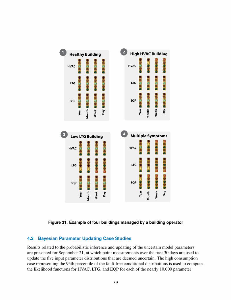
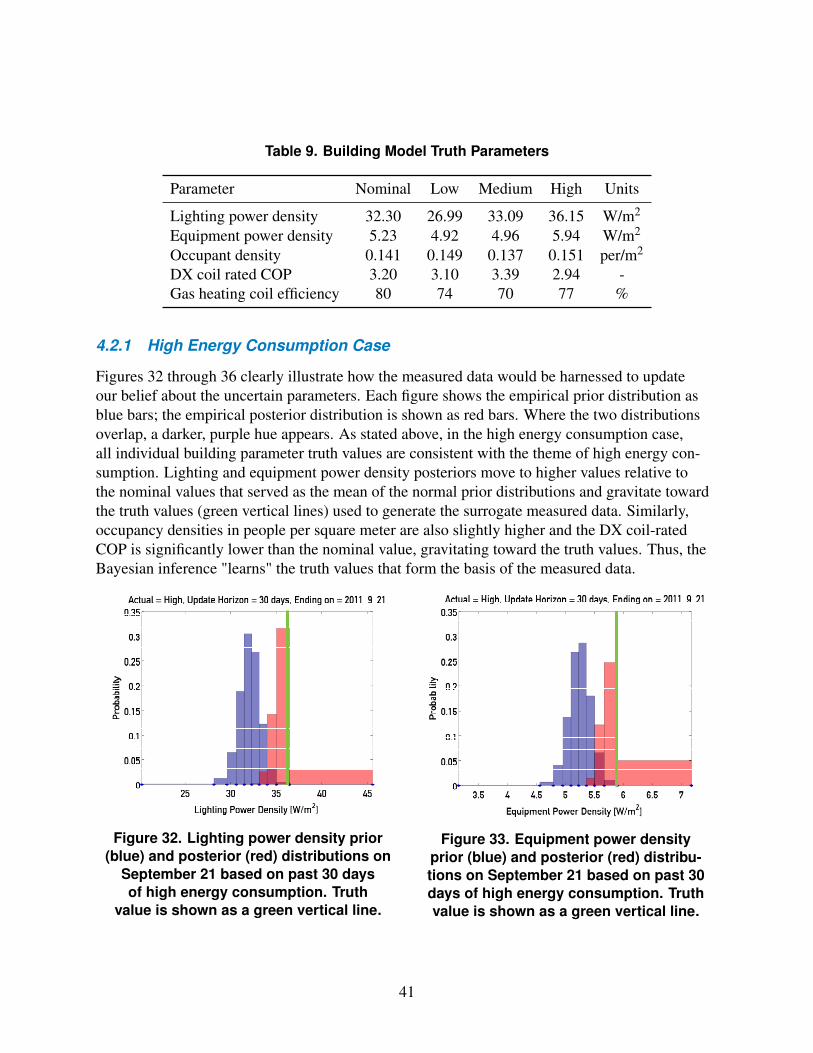
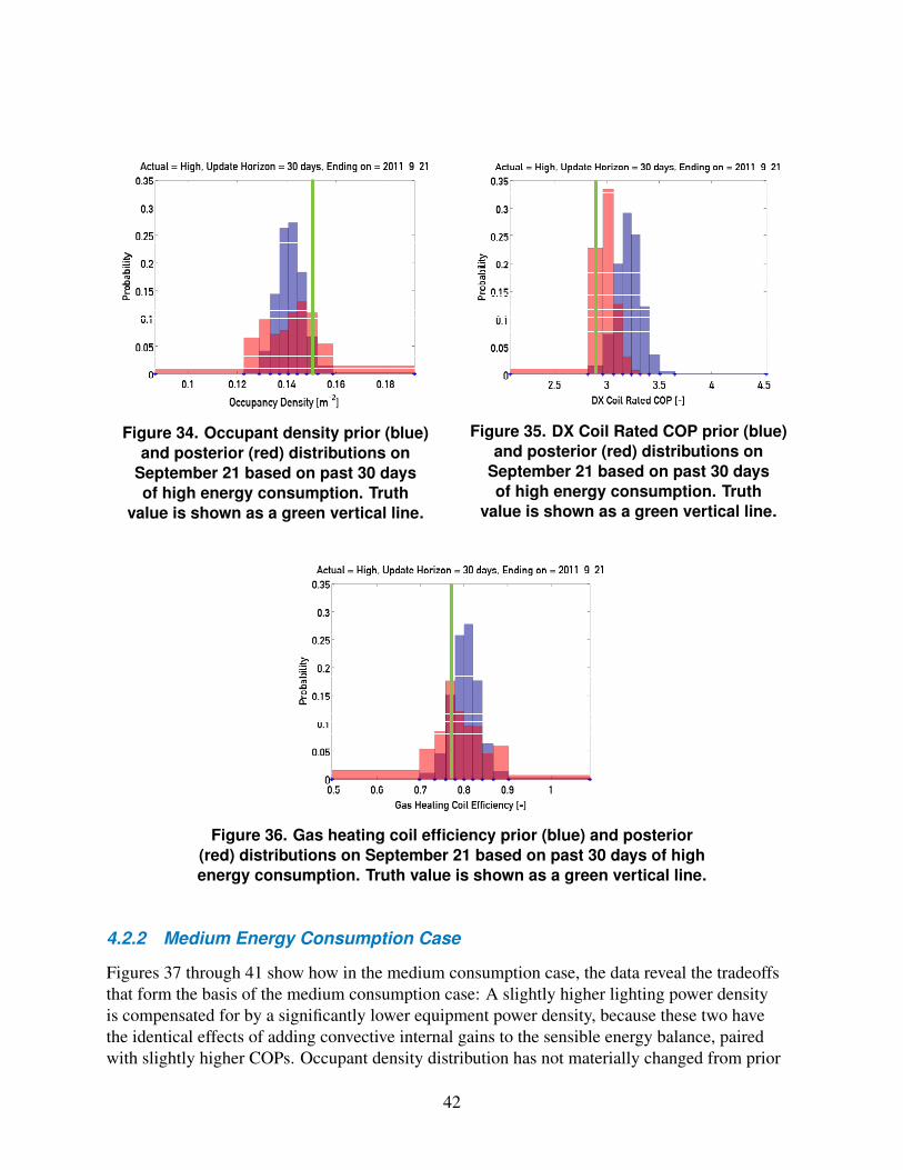
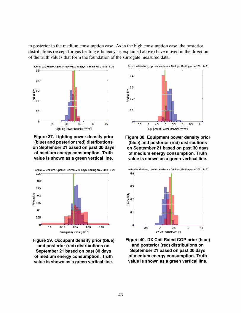
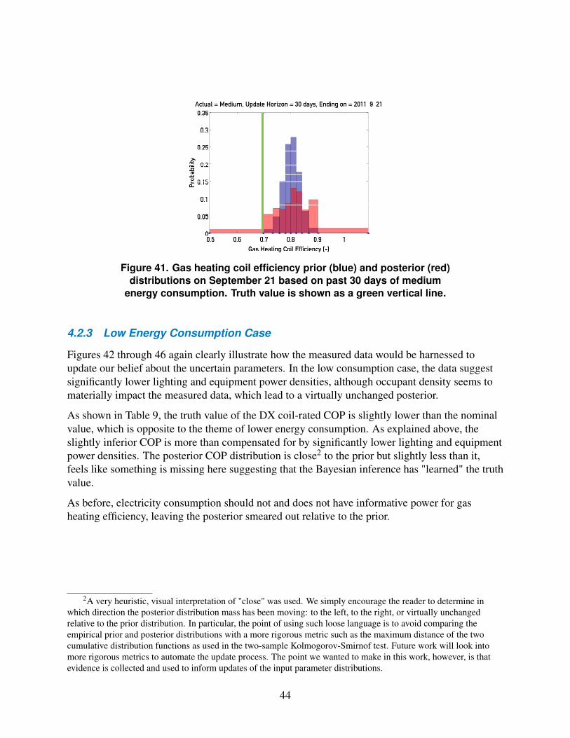
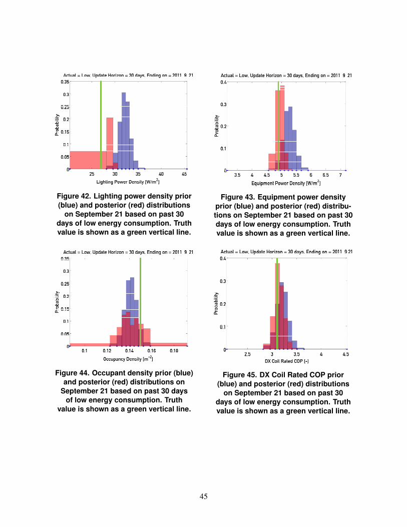
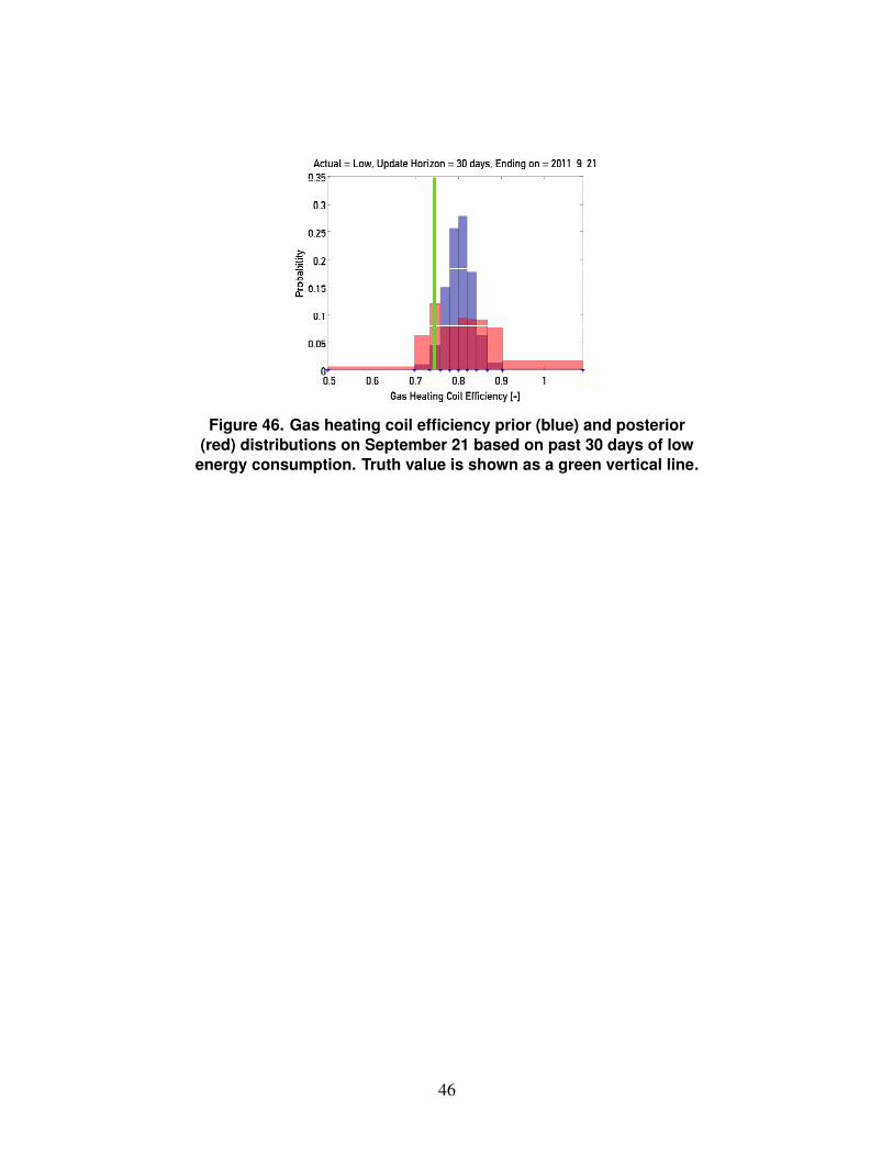