An End-to End Business Model for Retail Aggregation

of Responsive Load to Produce Wholesale Demand Side Resources

Shmuel S. Oren University of California, Berkeley

CERT Project Review Meeting Cornell University August, 6-7, 2013

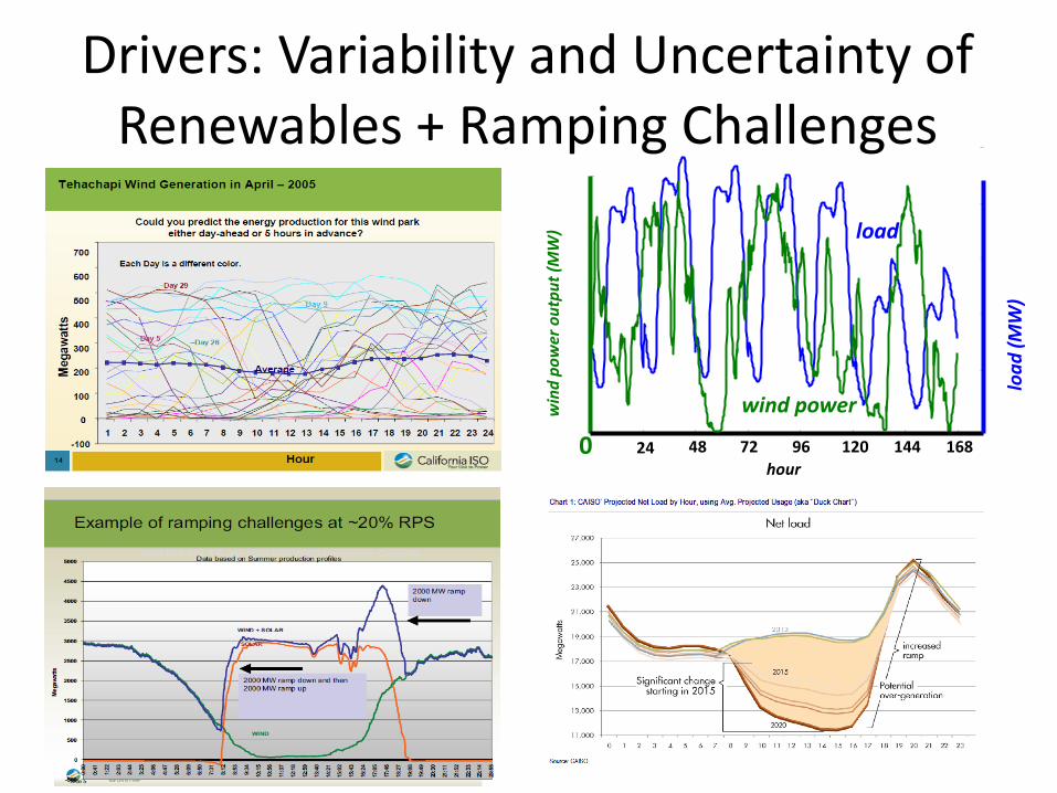
Drivers: Variability and Uncertainty of Renewables + Ramping Challenges

0

win

d po

wer

out

put (

MW

)

24 48 72 96 120 144 168

load

(MW

)

hour

wind power

load

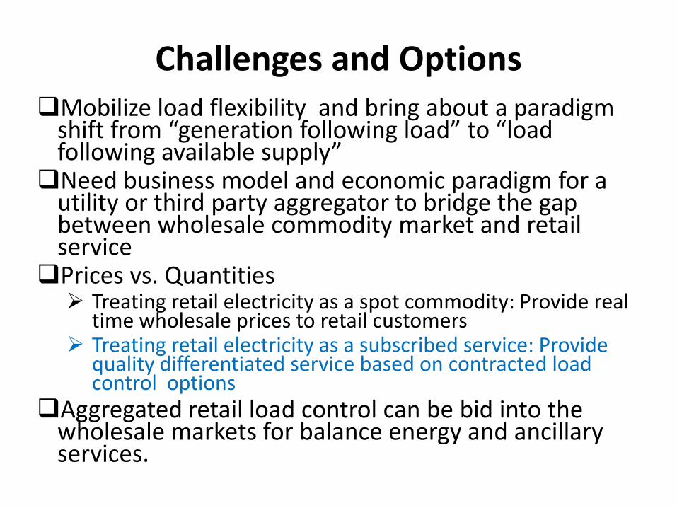
Challenges and Options Mobilize load flexibility and bring about a paradigm

shift from “generation following load” to “load following available supply” Need business model and economic paradigm for a

utility or third party aggregator to bridge the gap between wholesale commodity market and retail service Prices vs. Quantities Treating retail electricity as a spot commodity: Provide real

time wholesale prices to retail customers Treating retail electricity as a subscribed service: Provide

quality differentiated service based on contracted load control options

Aggregated retail load control can be bid into the wholesale markets for balance energy and ancillary services.

Rationale Treating electricity as a commodity works well at

wholesale level but retail customers would rather think of electricity as a service.

Quality differentiated service and optional price plans are common in other service industries (air transportation, cell phone, insurance) Customers have experience with choosing between

alternative service contracts Conjecture: Customers prefer uncertainty in service rather

than uncertain prices While RT price response can be automated it still puts

the burden on the customer

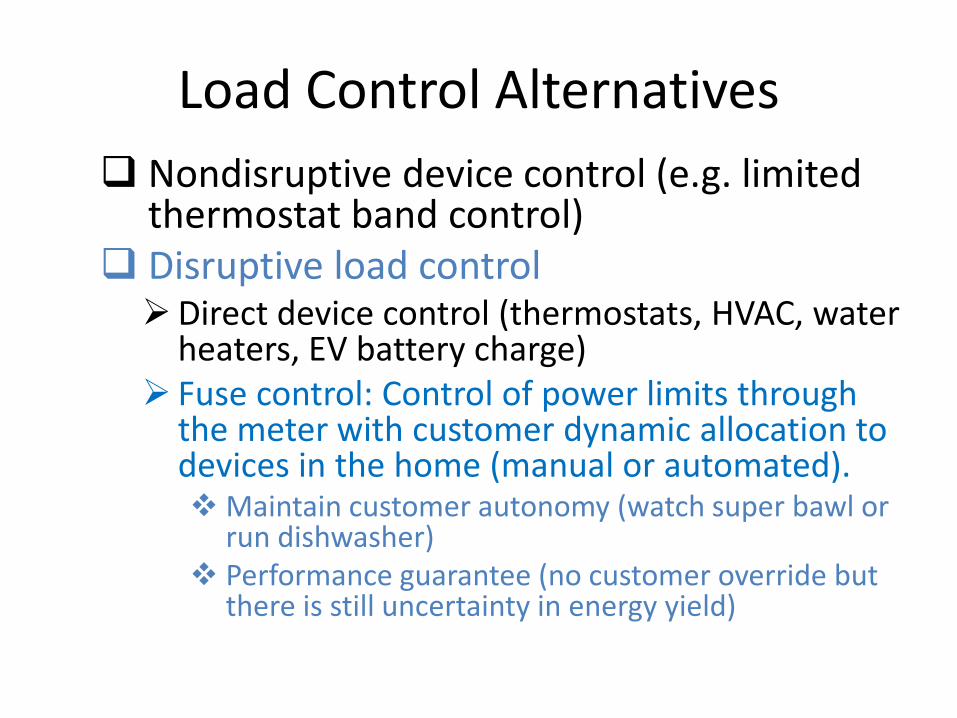
Load Control Alternatives Nondisruptive device control (e.g. limited

thermostat band control) Disruptive load control Direct device control (thermostats, HVAC, water

heaters, EV battery charge) Fuse control: Control of power limits through

the meter with customer dynamic allocation to devices in the home (manual or automated). Maintain customer autonomy (watch super bawl or

run dishwasher) Performance guarantee (no customer override but

there is still uncertainty in energy yield)

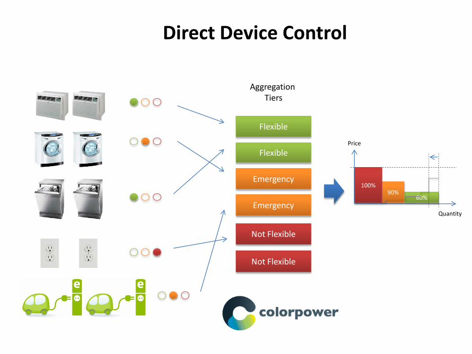
Flexible

Flexible

Emergency

Emergency

Not Flexible

Not Flexible

Aggregation Tiers

60% 90%

100%

Price

Quantity

Direct Device Control

Aggregator

Stratification of Demand into Service Priorities

Fuse KW

WTP

$/K

W

Aggregator

Prob. of Curtail.

Pay

$/K

W/Y

r.

Prob. of Curtail.

KWh

Curt

al.

Curtailment Controller

Yield Stats

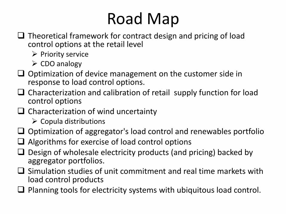
Road Map Theoretical framework for contract design and pricing of load

control options at the retail level Priority service CDO analogy

Optimization of device management on the customer side in response to load control options.

Characterization and calibration of retail supply function for load control options

Characterization of wind uncertainty Copula distributions

Optimization of aggregator's load control and renewables portfolio Algorithms for exercise of load control options Design of wholesale electricity products (and pricing) backed by

aggregator portfolios. Simulation studies of unit commitment and real time markets with

load control products Planning tools for electricity systems with ubiquitous load control.

FINANCIAL ANALOGY Bringing Financial Concepts to the Electricity Markets

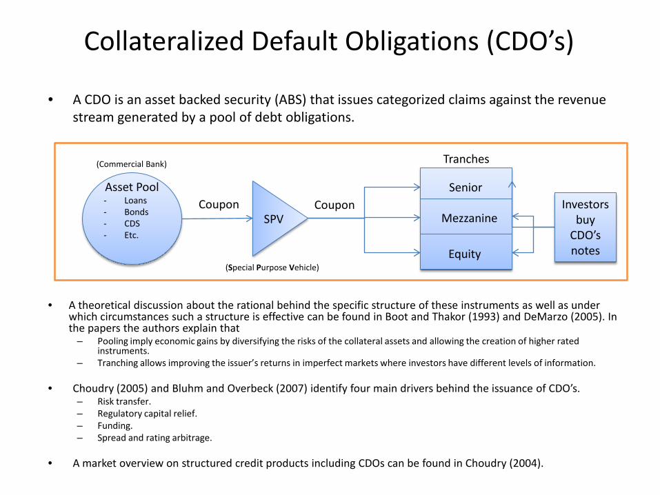
Collateralized Default Obligations (CDO’s)

• A theoretical discussion about the rational behind the specific structure of these instruments as well as under which circumstances such a structure is effective can be found in Boot and Thakor (1993) and DeMarzo (2005). In the papers the authors explain that

– Pooling imply economic gains by diversifying the risks of the collateral assets and allowing the creation of higher rated instruments.

– Tranching allows improving the issuer’s returns in imperfect markets where investors have different levels of information.

• Choudry (2005) and Bluhm and Overbeck (2007) identify four main drivers behind the issuance of CDO’s. – Risk transfer. – Regulatory capital relief. – Funding. – Spread and rating arbitrage.

• A market overview on structured credit products including CDOs can be found in Choudry (2004).

• A CDO is an asset backed security (ABS) that issues categorized claims against the revenue

stream generated by a pool of debt obligations.

Asset Pool - Loans - Bonds - CDS - Etc.

SPV

Senior

Mezzanine

Equity

Coupon Coupon

Tranches

Investors buy

CDO’s notes

(Commercial Bank)

(Special Purpose Vehicle)

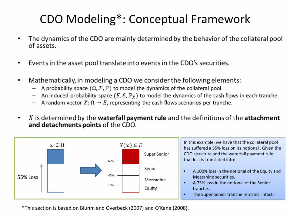
CDO Modeling*: Conceptual Framework

*This section is based on Bluhm and Overbeck (2007) and O'Kane (2008).

55% Loss 10%

40%

60%

Super Senior

Senior

Mezzanine

Equity

In this example, we have that the collateral pool has suffered a 55% loss on its notional . Given the CDO structure and the waterfall payment rule, that lost is translated into: • A 100% loss in the notional of the Equity and

Mezzanine securities. • A 75% loss in the notional of the Senior

tranche. • The Super Senior tranche remains intact.

The Analogy

Asset Pool - Loans - Bonds - CDS - Etc.

SPV

Senior

Mezzanine

Equity

Coupon Coupon

Tranches

Investors buy CDO’s

notes

• Parallel structural elements: – Pool of assets – pool of intermittent generation resources – the risk transfer from the originator to the investors – risk transfer from

generators to load – the segmentation of notes – load segmentation – the cash flow dynamics – service rules

Risk

Generation Pool

- Wind - Solar

Aggregator

100% Reliable

95% Reliable

90% Reliable

Power Power

Load Segments

Demand Side:

Houses & Buildings

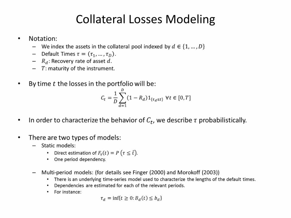
Collateral Losses Modeling

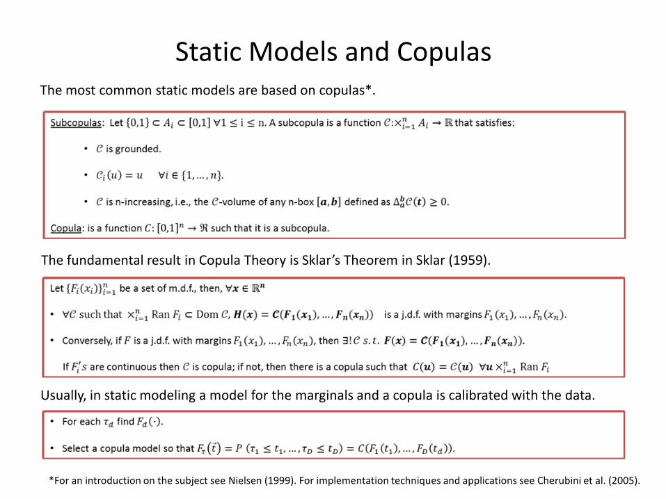
Static Models and Copulas The most common static models are based on copulas*.

The fundamental result in Copula Theory is Sklar’s Theorem in Sklar (1959).

*For an introduction on the subject see Nielsen (1999). For implementation techniques and applications see Cherubini et al. (2005).

Usually, in static modeling a model for the marginals and a copula is calibrated with the data.

CALIBRATION EXERCISE Applying Copula Models to Describe Wind Power Production

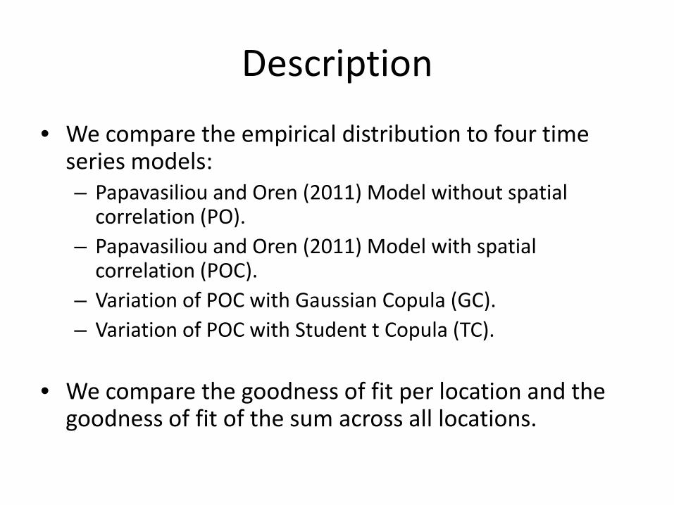
Description

• We compare the empirical distribution to four time series models: – Papavasiliou and Oren (2011) Model without spatial

correlation (PO). – Papavasiliou and Oren (2011) Model with spatial

correlation (POC). – Variation of POC with Gaussian Copula (GC). – Variation of POC with Student t Copula (TC).

• We compare the goodness of fit per location and the

goodness of fit of the sum across all locations.

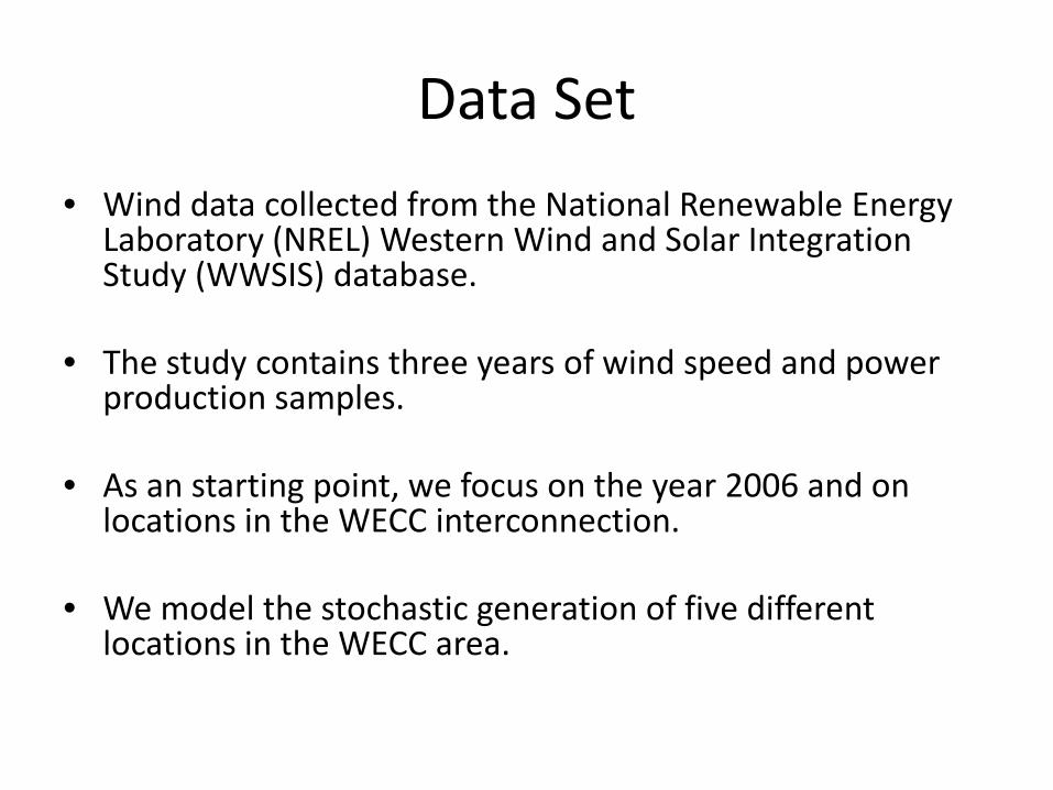
Data Set • Wind data collected from the National Renewable Energy

Laboratory (NREL) Western Wind and Solar Integration Study (WWSIS) database.

• The study contains three years of wind speed and power production samples.

• As an starting point, we focus on the year 2006 and on locations in the WECC interconnection.

• We model the stochastic generation of five different locations in the WECC area.

Schematic of WECC Interconnection

Source: Papavasiliou and Oren (2011).

Almont

Solano

Tehachapi

Clark County

Imperial

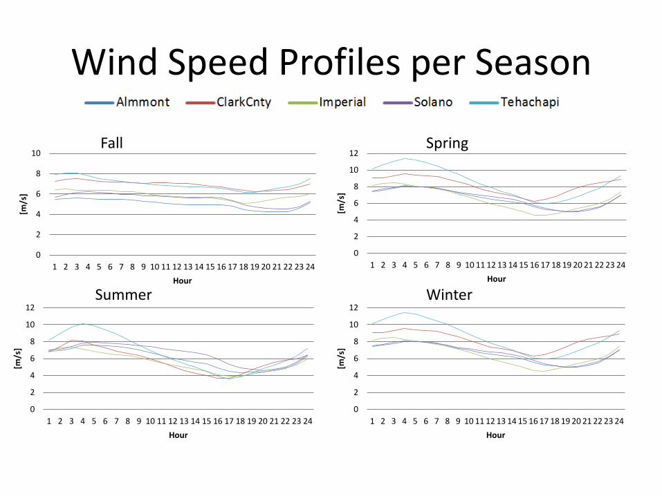
Wind Speed Profiles per Season

0

2

4

6

8

10

1 2 3 4 5 6 7 8 9 10 11 12 13 14 15 16 17 18 19 20 21 22 23 24

[m/s

]

Hour

0

2

4

6

8

10

12

1 2 3 4 5 6 7 8 9 10 11 12 13 14 15 16 17 18 19 20 21 22 23 24

[m/s

]

Hour

0

2

4

6

8

10

12

1 2 3 4 5 6 7 8 9 10 11 12 13 14 15 16 17 18 19 20 21 22 23 24

[m/s

]

Hour

0

2

4

6

8

10

12

1 2 3 4 5 6 7 8 9 10 11 12 13 14 15 16 17 18 19 20 21 22 23 24

[m/s

]

Hour

Fall Spring

Summer Winter

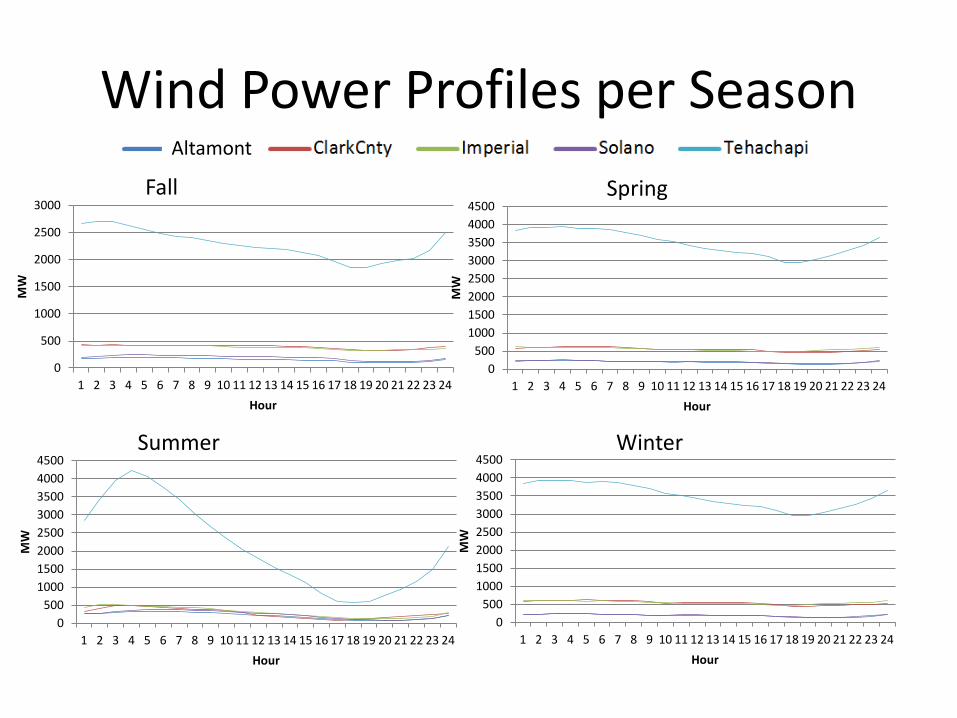
Wind Power Profiles per Season Fall Spring

Summer Winter

0

500

1000

1500

2000

2500

3000

1 2 3 4 5 6 7 8 9 10 11 12 13 14 15 16 17 18 19 20 21 22 23 24

MW

Hour

0 500

1000 1500 2000 2500 3000 3500 4000 4500

1 2 3 4 5 6 7 8 9 10 11 12 13 14 15 16 17 18 19 20 21 22 23 24

MW

Hour

0 500

1000 1500 2000 2500 3000 3500 4000 4500

1 2 3 4 5 6 7 8 9 10 11 12 13 14 15 16 17 18 19 20 21 22 23 24

MW

Hour

0 500

1000 1500 2000 2500 3000 3500 4000 4500

1 2 3 4 5 6 7 8 9 10 11 12 13 14 15 16 17 18 19 20 21 22 23 24

MW

Hour

Altamont

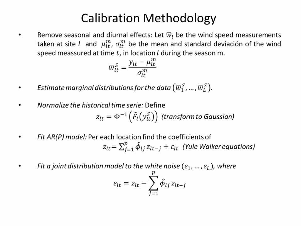
Calibration Methodology

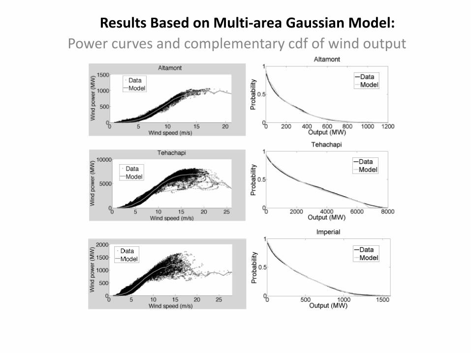
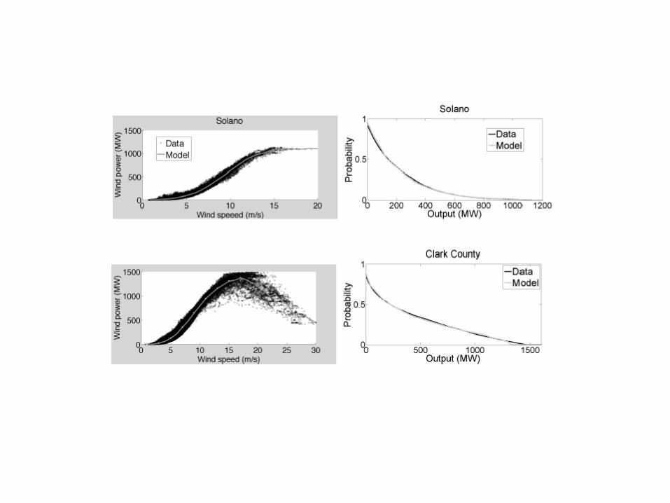
Results Based on Multi-area Gaussian Model: Power curves and complementary cdf of wind output

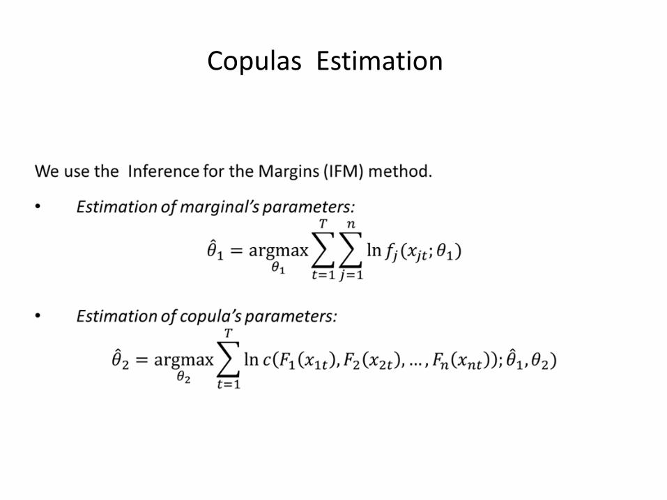
Copulas Estimation

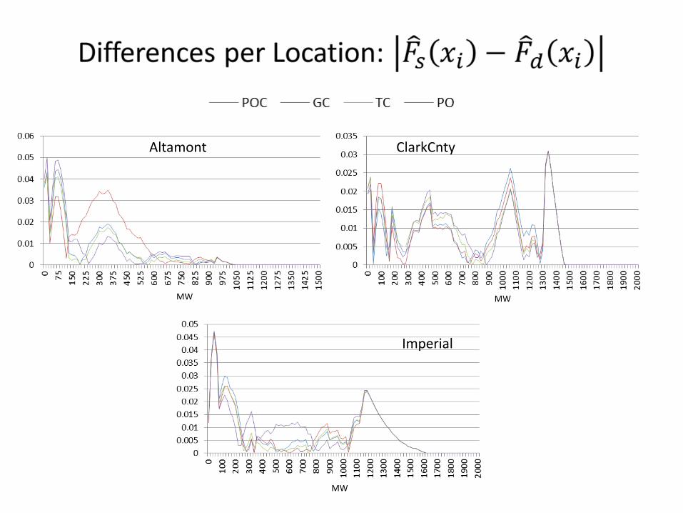
Altamont ClarkCnty

Imperial

MW MW

MW

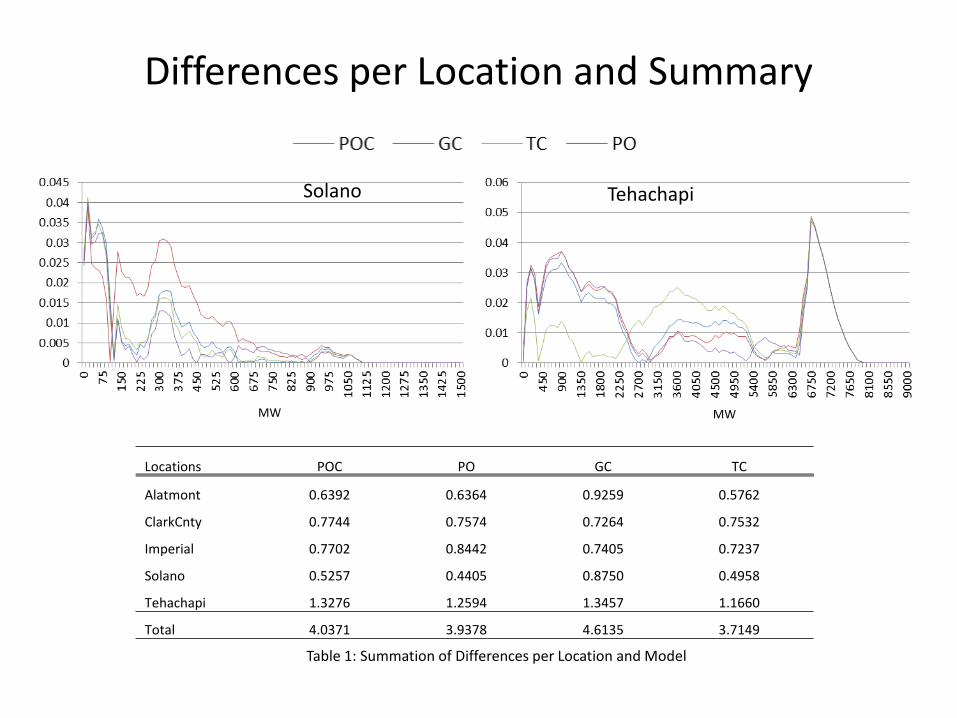
Differences per Location and Summary

Solano Tehachapi

Locations POC PO GC TC

Alatmont 0.6392 0.6364 0.9259 0.5762

ClarkCnty 0.7744 0.7574 0.7264 0.7532

Imperial 0.7702 0.8442 0.7405 0.7237

Solano 0.5257 0.4405 0.8750 0.4958

Tehachapi 1.3276 1.2594 1.3457 1.1660

Total 4.0371 3.9378 4.6135 3.7149

Table 1: Summation of Differences per Location and Model

MW MW

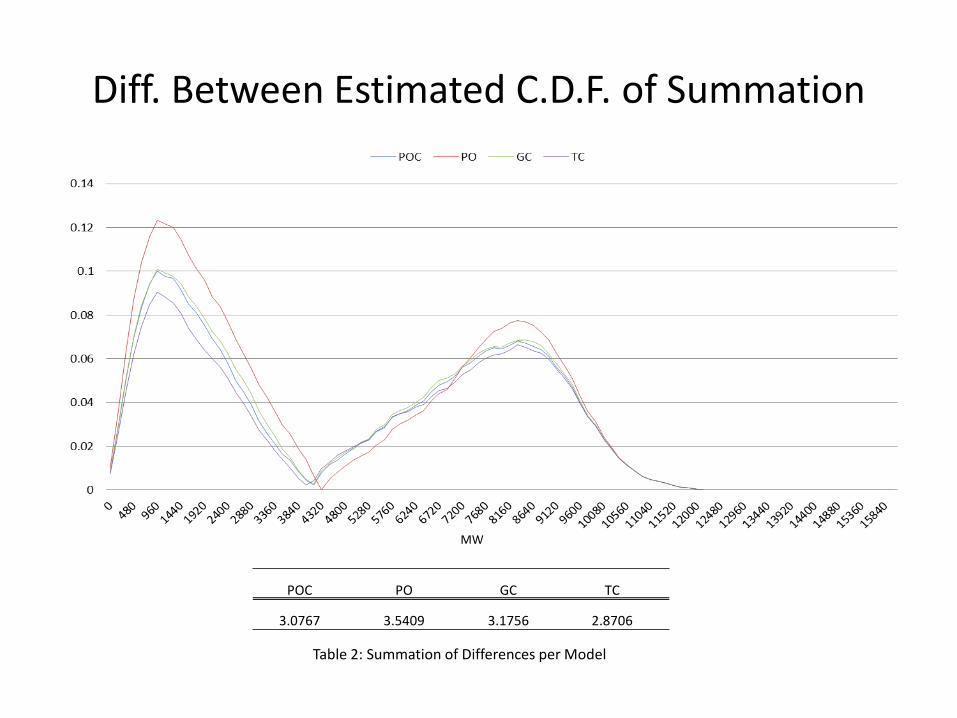
Diff. Between Estimated C.D.F. of Summation

Table 2: Summation of Differences per Model

POC PO GC TC

3.0767 3.5409 3.1756 2.8706

MW

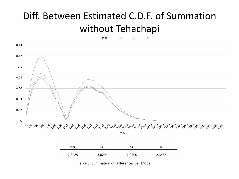
Diff. Between Estimated C.D.F. of Summation without Tehachapi

Table 3: Summation of Differences per Model

POC PO GC TC

2.3489 3.0291 2.2700 2.3486

MW

RETAIL CONTRACT DESIGN

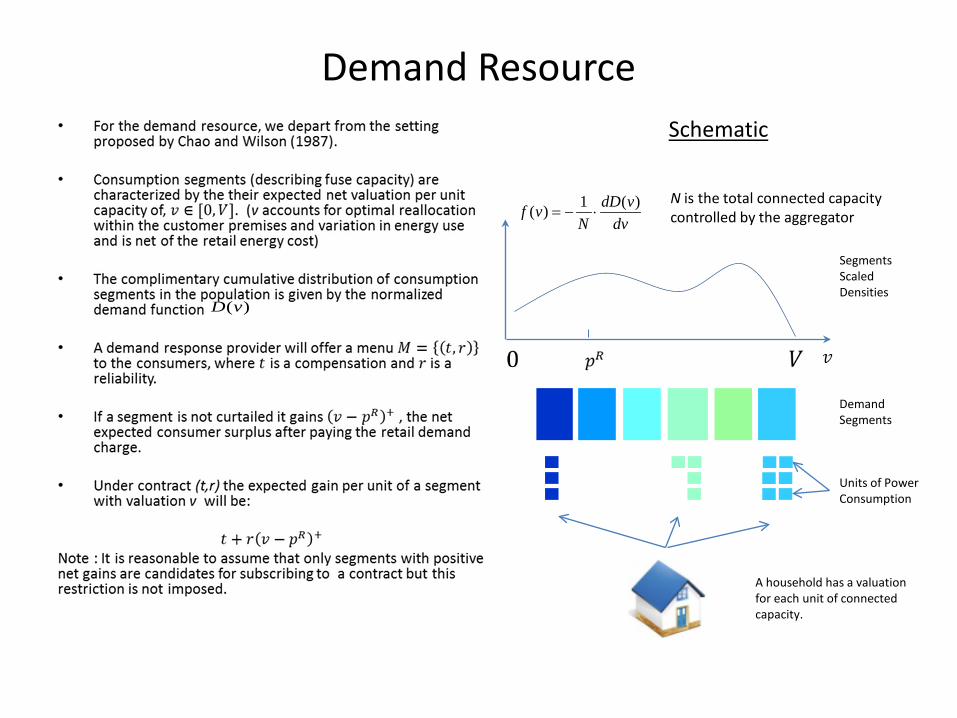
Demand Resource

Demand Segments

Units of Power Consumption

Segments Scaled Densities

A household has a valuation for each unit of connected capacity.

Schematic

( )D v

1 ( )( ) dD vf vN dv

= − ⋅N is the total connected capacity controlled by the aggregator

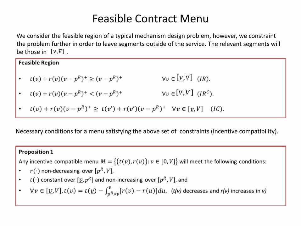
Feasible Contract Menu We consider the feasible region of a typical mechanism design problem, however, we constraint the problem further in order to leave segments outside of the service. The relevant segments will be those in .

Necessary conditions for a menu satisfying the above set of constraints (incentive compatibility).

[ , ]v v

[ , ]v v

[ , ]v V

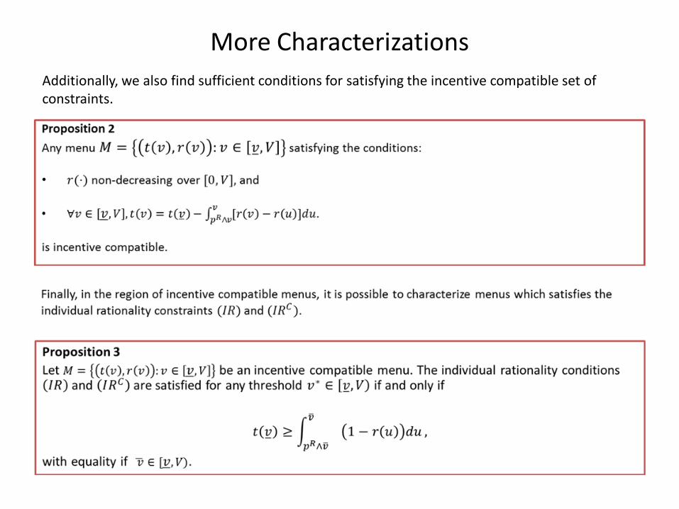
More Characterizations Additionally, we also find sufficient conditions for satisfying the incentive compatible set of constraints.

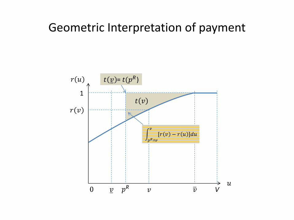
Geometric Interpretation of payment

V

1

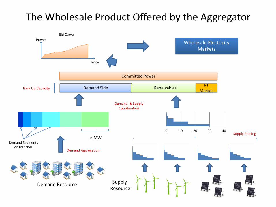
The Wholesale Product Offered by the Aggregator

0 10 20 30 40

Demand Resource Supply Resource

Demand Side

Committed Power

Demand Segments or Tranches

Demand Aggregation

Supply Pooling

Demand & Supply Coordination

Wholesale Electricity Markets

Power

Price

Bid Curve

Renewables Back Up Capacity RT

Market

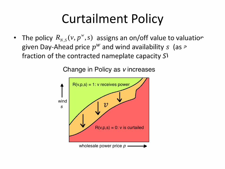
Curtailment Policy , ( , , )w

N SR v p s

Reliability r(v)

, ( , ( ), ( )) () )( WN SR v p s Pr dv ω ω ω= ∫

, ( , , ) ( ,( ) )N SR v p s h p s d sr v pd= ∫∫

, ( , , )wN SR v p s

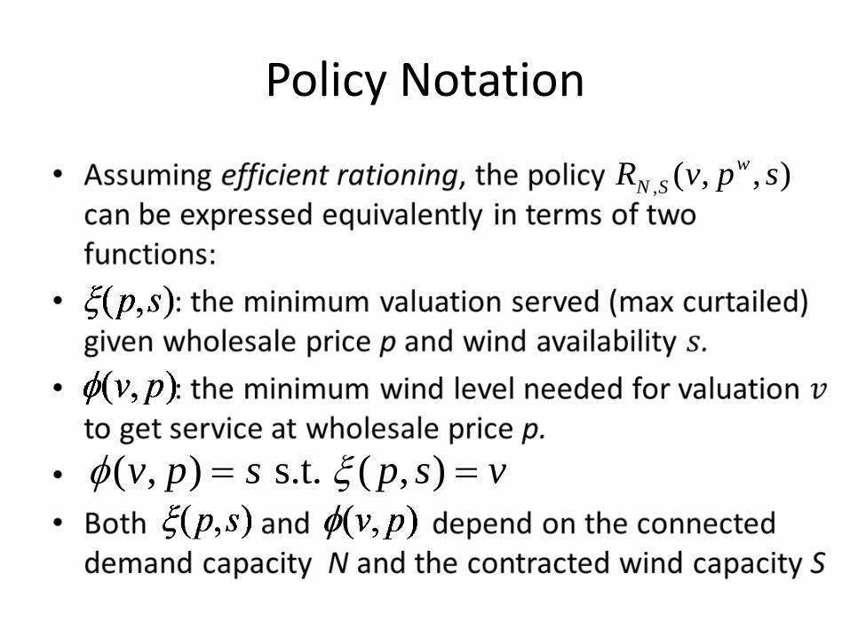
Policy Notation

( , ) s.t. ( , )v p s p s vφ ξ= =

, ( , , )wN SR v p s

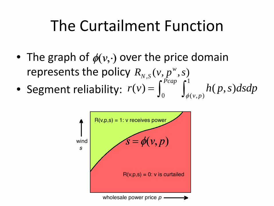
• The graph of over the price domain represents the policy

• Segment reliability:

1

0 ( , )) ( , )(

Pcap

v ph p s dsdr pv

φ= ∫ ∫

The Curtailment Function

, ( , , )wN SR v p s

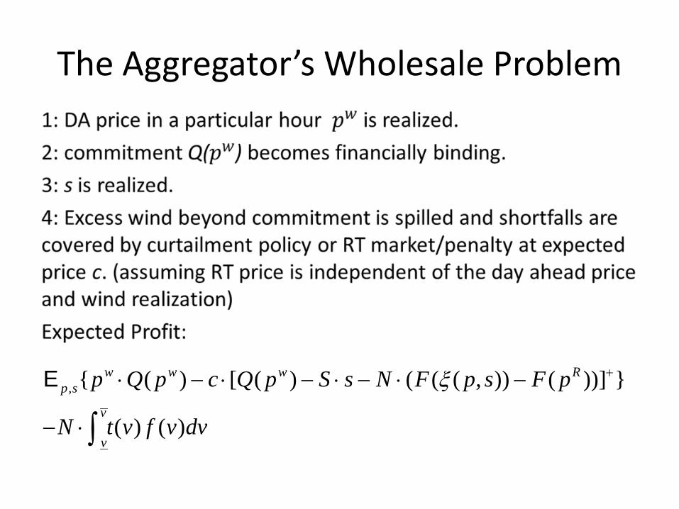
The Aggregator’s Wholesale Problem

, [{ ( ) ( , )( ) ( ( }

( ) ( )

) ( ))]w ww Rp s

v

v

p c Q p S s N F

t v f

Q p s

v d

p F p

vN

ξ +⋅ − ⋅ − ⋅⋅ − −

− ⋅ ∫

E

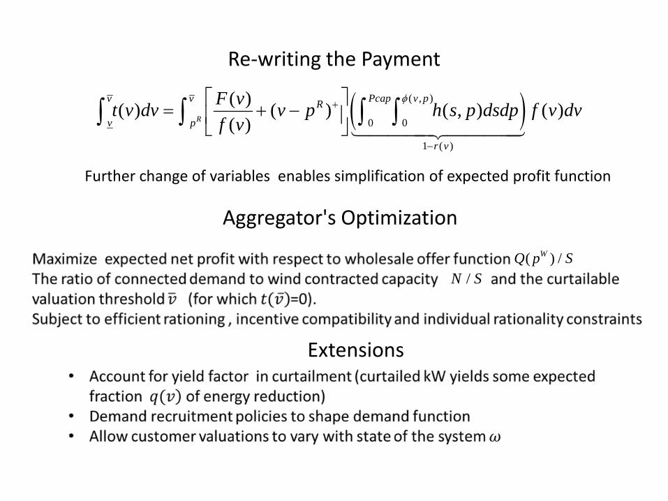
Re-writing the Payment

( )1 ( )

( , )

0 0) ( )( )( ) ( ( , )

( )R

v v Pcap v pR

p

v

v

r

fF vt v dv v p h s p dsdpf

vv

v dφ

−

+ = + −

∫ ∫ ∫ ∫

Aggregator's Optimization

( ) /WQ p S/N S

Further change of variables enables simplification of expected profit function

Extensions

References • T.R. Bielecki and M. Rutkowski. "Credit Risk: Modeling, Valuation and Hedging." Springer, 2004.

• E. Bitar, P. Khargonekar, K. Poolla, R. Rajagopal, P. Varaiya, and F. Wu, “Selling random wind,” 45th Hawaii

International Conference on System Science (HICSS), 2012.

• C. Bluhm and L. Overbeck. "Semi-Analytic Approaches to CDO Modeling." Economic Notes 33, No. 2, pp. 233-255, 2004.

• C. Bluhm and L. Overbeck. "Comonotonic Default Quote Paths for Basket Evaluation." Risk 18 (8), pp. 67-71, 2005.

• C. Bluhm and L. Overbeck. "Structured Credit Portfolio Analysis, Baskets and Cdos." Chapman & Hall/CRC, 2007.

• A. Boot and A. Thakor. “Security Design." The Journal of Finance, Vol. 48, No. 4 , pp. 1349-1378, 1993.

• H. Chao and R. Wilson. “Priority Service: Pricing, Investment, and Market Organization.” American Economic Review Vol. 77, No. 5, pp. 899–916, 1987.

• G. Cherubini, W. Vecchiato, E. Luciano. “Copula Models in Finance.” John Wiley & Sons, New-York, 2004.

• M. Choudry. "Structured Credit Products: Credit Derivatives and Synthetic Securitization." John Wiley & Sons, 2004.

• M. Choudry. "Fixed-Income Securities and Derivatives Handbook: Analysis and Valuation." Bloomberg Professional, 2005 .

• P. DeMarzo. "The Pooling and Tranching of Securities: A Model of Informed Intermediation." The Review of Financial Studies, Vol 18, pp. 1-35, 2005.

References • C. Donnelly and P. Embrechts. “The devil is in the tails: actuarial mathematics and the subprime mortgage

crisis.” ASTIN Bulletin Vol. 40, No. 1, 1-33, 2010.

• C. C. Finger. "A Comparison of Stochastic Default Rate Models." RiskMetrics Journal, Vol. 1, 2000.

• I. O. Filiz, X. Guo, J. Morton, B. Sturmfels. "Graphical Models for Correlated Defaults." Mathematical Finance, Vol. 22, Issue 4, pp. 621–644, 2012.

• M. F. Hellwig. “Systemic risk in the financial sector: an analysis of the subprime-mortgage financial crisis.” De Economist, Vol. 157 No. 2, pp. 129-207, 2009.

• W. J. Morokoff. "Simulation Methods for Risk Analysis of Collateralized Debt Obligations." Moody’s KMV, 2003.

• R. Nelsen, An Introduction to Copulas, Springer-Verlag NewYork, Inc., 1999.

• D. O'Kane. "Modeling Single-Name and Multi-Name Credit Derivatives." Wiley, 2008. • A. Papavasiliou, S. S. Oren, R. P. O'Neill. (2011) “Reserve Requirements for Wind Power Integration: A

Scenario-Based Stochastic Programming Framework”, IEEE Transactions on Power Systems, Vol. 26, No. 4.

• A. Papavasiliou, S. S. Oren, Multi-Area Stochastic Unit Commitment for High Wind Penetration in a Transmission Constrained Network, accepted for publication in Operations Research, 2011.

• M. Sklar, “Fonctions de répartition à n dimensions et leurs marges,” Publications de l’Institut de Statistique de L’ Université de Paris, vol. 8, pp. 229–231, 1959.

• O.A. Vasicek. “The loan loss distribution.” Technical report. KMV Corporation, 1997.