An empirical test for the identifying assumptions

of the Blanchard and Quah (1989) model

Hyeon-seung Huh

School of Economics Yonsei University

262 Seongsanno, Seodaemun-Gu Seoul 120-749

Korea Tel: +82-2-2123-5499

Email: hshuh@yonsei.ac.kr

Abstract

In their vector autoregression model, Blanchard and Quah (1989) employed as identifying assumptions uncorrelatedness between aggregate supply and aggregate demand shocks and the long-run output neutrality condition. This paper examines the empirical consistency of these assumptions with actual data. To derive a testable form, the Blanchard and Quah model is transformed into a cointegration representation that produces identical results. This alternative setup is extended to allow for a joint test of the uncorrelatedness and long-run output neutrality assumptions. Empirical results indicate that the joint assumptions when taken together are accepted by the data for Japan and the U.S. but rejected for Germany. Further analysis reveals that the imposition of the long-run output neutrality assumption is responsible for such rejection in Germany.

Key words: Blanchard and Quah; Cointegration; Shocks; Identifying assumptions

JEL classification: C32; C52; E32

Acknowledgement: The author thanks the Department of Economics at the University of Washington for its hospitality. This work was supported by the National Research Foundation of Korea Grant funded by the Korean Government (NRF-2010-013-B00007).

2

1. Introduction

In an influential study, Blanchard and Quah (BQ, 1989) developed a vector autoregression

(VAR) model that identifies the effects of aggregate supply (AS) and aggregate demand (AD)

shocks on real output and the unemployment rate. Two assumptions are employed for

identification of structural shocks. The first assumption is that AS and AD shocks are

mutually uncorrelated. The rationale for this is that structural shocks are primitive, exogenous

forces and hence have no common causes. The second assumption is that an AD shock has no

long-run effects on real output. This is based on the long-run output neutrality condition,

according to which the AS curve is vertical and independent of AD factors in the long run, so

that only AS shocks can have long-run effects on real output.1

Both assumptions are not without criticism, however. Cover et al. (2006) suggest

reasons why AS and AD shocks may be correlated with each other. Shiller (1986) and

Pesaran and Smith (1998) argue that assuming uncorrelatedness between shocks may not be

reasonable in many econometric applications of the structural VAR methodology.2 Cooley

and Dwyer (1998) and Giordani (2004) provide examples in which this assumption produces

specification errors and biased impulse response estimators. Campbell and Mankiw (1987)

and Keating (2005) summarize a variety of possible mechanisms through which aggregate

1 Uncorrelatedness between structural shocks is a common assumption that most structural VAR studies impose in the identification process. The absence of this assumption entails n(n–1)/2 additional restrictions for exact identification in an n-variable model. The long-run output neutrality assumption has also been extensively adopted for identifying AS and AD shocks individually. 2 The structural shocks are generally permitted to correlate with each other in the simultaneous equation macroeconometric model (e.g. the Cowles Commission approach). The dynamic structure is restricted, instead, for identification, typically by excluding contemporaneous and lagged regressors. See Pagan and Robertson

3

demand shocks may have long-run effects on the level of real output. In fact, BQ

acknowledged some of these effects, such as hysteresis (à la Blanchard and Summers, 1986)

and endogenous models of growth. The hysteresis hypothesis suggests that the natural

unemployment rate depends on the past levels of the unemployment rate, allowing aggregate

demand shocks to influence the natural rate and hence, the level of real output in the long

run.3 Within the context of an endogenous growth model, any aggregate demand shock can

have long-run effects on the level of real output as long as it produces temporary changes in

the amount of resources allocated to growth (Stadler, 1986; King et al., 1988).

The present paper examines the extent to which the uncorrelatedness and long-run

output neutrality assumptions of the BQ model are consistent with actual data. This issue is

important because the model implications are dependent on the adequacy of the assumptions

in use. Where the assumptions are inconsistent with data, their imposition may result in

misrepresentation of the true dynamic structure of the model. Nevertheless, the

uncorrelatedness and long-run output neutrality assumptions in the BQ model have rarely

been evaluated for their empirical relevance. The main reason is that the two assumptions are

exact-identifying restrictions, and hence they cannot be tested.

To derive a testable form, this paper presents the BQ model in a cointegration

framework. The starting point is that real output is difference-stationary and the

(1995) and Jacobs and Wallis (2005) for a comparison between this traditional approach and the VAR modeling. 3 For empirical applications, see Dolado and Jimeno (1997) and Astley and Yates (1999).

4

unemployment rate is stationary in levels. This implies that the two variables are cointegrated

where the unemployment rate itself is the cointegration relation. The corresponding vector

error correction model is structurally identified by using a procedure that decomposes the

shocks into those with permanent effects and those with transitory effects. The results are

exactly the same as those from the BQ model.4

The key feature is that this cointegration representation can be extended to allow for

relaxation of the two identifying assumptions underlying the BQ model. The correlation

between AS and AD shocks and the long-run response of real output to an AD shock are not

restricted but determined freely by the data. Thus, comparison of the results with those from

the BQ model can be used as a joint test for evaluating the empirical relevance of the two

identifying assumptions with respect to the data. This paper also introduces two companion

representations. One allows for correlation between AS and AD shocks under the long-run

output neutrality assumption. The other admits that an AD shock can have potentially long-

run effects on real output under the uncorrelatedness assumption between AS and AD shocks.

These models are utilized for examining the question of which assumption, i.e.

uncorrelatedness of the structural shocks or long-run output neutrality, has greater impact

when the joint assumptions taken together are rejected by the data.

The remainder of this paper is organized as follows. Section 2 presents a cointegration

4 Englund et al. (1994) and Fry and Pagan (2005) gave a general indication of this possibility, but they did not prove equivalence between the BQ model and its cointegration representation, due to a different focus.

5

representation of the BQ model and an extension is made to allow for relaxation of the

uncorrelatedness and long-run output neutrality assumptions. Empirical applications to the

U.S., Germany, and Japan are provided in Section 3. Section 4 presents the two companion

models together with their empirical results. Section 5 concludes the paper. The appendix

formally proves equivalence between the BQ model and its cointegration representation.

2. A joint testing procedure

2-1. The Blanchard and Quah model

The Blanchard and Quah (BQ) model begins with estimation of a reduced-form VAR model

given as:

p pt yy,i t i yu,i t i 1t

i 1 i 1y f y f u e− −

= =Δ = Δ + +∑ ∑ (1)

p pt uy,i t i uu,i t i 2t

i 1 i 1u f y f u e− −

= == Δ + +∑ ∑ (2)

where ty is real output, tu is the unemployment rate, Δ is the first difference operator,

t 1t 2te (e ,e ) '= is a vector of reduced-form shocks and is iid with a mean of zero and a

covariance matrix of 't tE(e e ) = Ω .5 Let tz be the vector t t( y ,u ) 'Δ . The vector moving

average (VMA) representation for (1) and (2) can be expressed in compact form as:

t tz C(L)e= (3)

where 20 1 2C(L) C C L C L = + + + , 0C I= , i

ii 0C(1) C L∞== ∑ , and L is the lag operator.

5 The constant term is suppressed for the sake of illustration.

6

Subject to identification, a structural VMA representation corresponding to (3) is

given as:

t tz (L)= Γ ε (4)

where 20 1 2(L) L L Γ = Γ + Γ + Γ + , i

ii 0(1) L∞=Γ = Γ∑ , and t 1t 2t( , ) 'ε = ε ε is a vector of

structural shocks. Following BQ, 1tε and 2tε are denoted as an aggregate supply (AS)

shock and an aggregate demand (AD) shock, respectively. These are assumed to have a mean

of zero and a covariance matrix of the form:

12't t

12

1E( )

1σ⎛ ⎞

ε ε = Σ = ⎜ ⎟σ⎝ ⎠ (5)

where each structural shock is normalized to have unit variance without loss of generality.

From (3) and (4), the relationships between the reduced-form and structural parameters are:

0(L) C(L)Γ = Γ (6)

and

1t 0 te−ε = Γ . (7)

For exact identification of the structural shocks, the four parameters in 0Γ or 10−Γ

must be uniquely determined. The two identifying assumptions now come into action.

Uncorrelatedness between AS and AD shocks leads to 12 0σ = in (5), and then '0 0Γ Γ = Ω

in (7) yields three restrictions on 0Γ . The long-run output neutrality assumption implies that

the element (1,2) of the long-run impact matrix (1)Γ in (4) is zero. (1)Γ then becomes

lower triangular. This provides one remaining restriction on 0Γ by setting the (1,2) element

7

of 0C(1)Γ in (6) to zero. Accordingly, solving '0 0Γ Γ = Ω under long-run output neutrality

gives the four parameters in 0Γ .6 Once 0Γ is estimated, the impulse responses and the

forecast-error variances of the series can be computed from (6).

2-2. A cointegration representation of the Blanchard and Quah model

The BQ model can be cast in a cointegated VAR framework. This is possible because the

model assumes that real output is difference-stationary and the unemployment rate is

stationary in levels. One implication is that the two variables are cointegrated where the

unemployment rate itself is the cointegration relation, i.e. [0, 1]'β = . The error correction

term is given as:

t t'z uβ = (8)

and a vector error correction (VEC) representation for (1) and (2) may be written as:

p p 1t yy,i t i yu,i t i 1 t p 1t

i 1 i 1y g y g u u e

−− − −

= =Δ = Δ + Δ + α +∑ ∑ (9)

p p 1t uy,i t i uu,i t i 2 t p 2t

i 1 i 1u g y g u u e

−− − −

= =Δ = Δ + Δ + α +∑ ∑ (10)

where 1 2[ , ]'α = α α is a vector of error correction coefficients.

Let ts be the vector t t( y , u ) 'Δ Δ . The Granger Representation Theorem shows that

the VEC model in (9) and (10) can be inverted to obtain the VMA representation (for details,

see Engle and Granger, 1987):

6 An equivalent but simpler solution is to combine (6) and (7) as ' 'C(1) C(1) (1) (1)Ω = Γ Γ . Taking the Choleski

8

t ts D(L)e= (11)

where 20 1 2D(L) D D L D L = + + + , 0D I= , and

i 'ii 0D(1) D L ∞

⊥ ⊥== = β ψα∑ (12)

where 1 2[ , ]'⊥ ⊥ ⊥α = α α and 1 2[ , ]'⊥ ⊥ ⊥β = β β are vectors orthogonal to α and β ,

respectively (i.e. ' 0⊥α α = and ' 0⊥β β = ), ' 1( G(1) )−⊥ ⊥ψ = α β , and G(1) is the short-run

impact matrix of reduced-form shocks from (9) and (10), given by:

p p 1yy,i yu,ii 1 i 1

p p 1uy,i uu,ii 1 i 1

1 g gG(1)

g 1 g

−= =

−= =

⎡ ⎤− −⎢ ⎥= ⎢ ⎥− −⎢ ⎥⎣ ⎦

∑ ∑∑ ∑

.

A detailed derivation is found in Johansen (1991).

The presence of one cointegrating relationship in the model implies that one shock

exhibits permanent effects, whereas the other shock demonstrates only transitory effects.7

The first ( 1tε ) is designated as an AS shock and the second ( 2tε ) as an AD shock. This

interpretation is plausible in that the AS shock has permanent effects on real output but the

AD shock has only transitory effects. To decompose the shocks into those with permanent

effects and those with transitory effects, we employ the Beveridge and Nelson (1981)

procedure of a type proposed for VEC models by Mellander et al. (1992), Englund et al.

(1994), Levtchenkova et al. (1996), and Fisher et al. (2000). The model posits for the

relationship between the reduced-form and structural shocks of (7) that:

decomposition of C(1) C(1) 'Ω provides all estimates in (1)Γ , and hence 0Γ , from (6). 7 See King et al. (1991), Mellander et al. (1992), and Levtchenkova et al. (1996) for the implications of cointegration in the structural identification of VEC models.

9

'1

0 1'⊥−−

⎡ ⎤α⎢ ⎥Γ =⎢ ⎥α Ω⎣ ⎦

. (13)

Equation (13) is modified for each structural shock to have unit variance, which is given as:

'11

0 1 ' 11

⊥−− −

⎡ ⎤Λ α⎢ ⎥Γ =⎢ ⎥Φ αΩ⎣ ⎦

(14)

where 1 T '1 1− −

⊥ ⊥Λ Λ = α Ωα and ' ' 11 1

−Φ Φ = αΩ α .

Combining (7) and (14) reveals that '1 te⊥Λ α and 1 ' 1

1 te− −Φ αΩ are permanent AS

( 1tε ) and transitory AD ( 2tε ) shocks, respectively. It is also straightforward to show that

'' '1 1' 1 T

t t 0 0 1 ' 1 1 ' 11 1

E( ) I⊥ ⊥− −− − − −

⎡ ⎤ ⎡ ⎤Λ α Λ α⎢ ⎥ ⎢ ⎥ε ε = Γ ΩΓ = Ω =⎢ ⎥ ⎢ ⎥Φ αΩ Φ αΩ⎣ ⎦ ⎣ ⎦

. (15)

The correlation between AS and AD shocks is zero. The inverse matrix of 10−Γ is calculated

as:

' T0 1 1 −

⊥⎡ ⎤Γ = Ωα Λ αΦ⎣ ⎦ . (16)

The application of (6), (12), and (16) demonstrates that

' ' T 10 1 1 1(1) D(1) [ ] [ 0]− −

⊥ ⊥ ⊥ ⊥Γ = Γ = β ψα Ωα Λ αΦ = β ψΛ . (17)

As the implied cointegrating vector of [0, 1]'β = gives [1, 0]'⊥β = , (1)Γ of

dimension (2x2) becomes:

11 0(1)

0 0

−⎡ ⎤ψΛΓ = ⎢ ⎥⎢ ⎥⎣ ⎦

. (18)

Equation (18) confirms that the AS shock has permanent effects on real output, while the AD

shock has only transitory effects. Both shocks have transitory effects on the unemployment

10

rate, which is consistent with the assumption that the rate is stationary in levels. This

cointegration representation matches the BQ model exactly, and they generate identical

results. A formal proof is provided in the Appendix.

2-3. Relaxation of the uncorrelatedness and long-run output neutrality assumptions

Now we present an extended model that can be used to jointly test the empirical relevance of

the uncorrelatedness and long-run output neutrality assumptions. This model, denoted as BQ-

E, shares the VEC representation in (9) and (10) but takes a different decomposition for the

identification of structural shocks. Specifically, it is assumed that

'21

0 1 ' 12

⊥−− −

⎡ ⎤Λ β⎢ ⎥Γ =⎢ ⎥Φ αΩ⎣ ⎦

, (19)

and its inverse is calculated as:

' 1 1 ' 1 10 2 2[ ( ) ( ) ]− − − −

⊥ ⊥ ⊥Γ = Ωα Λ β Ωα β Φ αΩ β (20)

where 1 T '2 2− −

⊥ ⊥Λ Λ = β Ωβ and ' ' 12 2

−Φ Φ = αΩ α . From (7), '2 te⊥Λ β and 1 ' 1

2 te− −Φ αΩ

correspond to AS and AD shocks, respectively.

The covariance matrix of the structural shocks is:

' T2 2' 1 T

t t 0 0 ' T2 2

1E( )

1

−⊥− −

−⊥

⎡ ⎤Λ β αΦ⎢ ⎥ε ε = Γ ΩΓ =⎢ ⎥Λ β αΦ⎣ ⎦

. (21)

The long-run impact matrix of the structural shocks is obtained from (12) and (20) as:

' ' 1 ' 1 ' 1 10 2 2(1) D(1) [ ( ) ( ) ]− − − −

⊥ ⊥ ⊥ ⊥ ⊥ ⊥ ⊥Γ = Γ = β ψα Ωα Λ β Ωα β ψα β Φ αΩ β . (22)

11

On using [1, 0]'⊥β = , (22) is summarized as:

' ' 1 ' 1 ' 1 12 2

0( ) ( )(1) D(1)

0 0

− − − −⊥ ⊥ ⊥ ⊥ ⊥⎡ ⎤ψα Ωα Λ β Ωα ψα β Φ αΩ βΓ = Γ = ⎢ ⎥

⎢ ⎥⎣ ⎦. (23)

Equations (21) and (23) show key differences from the BQ model. The correlation between

two structural shocks is not restricted to being zero, nor is the long-run effect of the AD shock

on real output. Instead, they are allowed to be determined freely by the data. This provides

one way of jointly testing their empirical relevance. If results from the BQ model are

different from those of the BQ-E model, this can be taken as evidence that the joint

assumptions of uncorrelatedness and long-run output neutrality, taken together, are not

consistent with the actual data. If the results do not differ, the two assumptions are

empirically supported, justifying their use in the BQ model. A more detailed discussion will

be provided in the section to follow.

If '⊥β α in (21) and '

⊥α β in (23) are zero, both the uncorrelatedness and the long-

run output neutrality become valid for the BQ-E model.8 This occurs when real output is

weakly exogenous to the cointegrating vector in the VEC model of (9) and (10), i.e.

2[0, ]'α = α and hence 1[ , 0]'⊥ ⊥α = α .9 In fact, the BQ and BQ-E models coincide exactly.

This can be easily demonstrated by noting that when 2[0, ]'α = α , ⊥α can be

reparameterized as [1, 0]'⊥α = .10 Because ⊥ ⊥α = β , all equations in the BQ-E model

8 Note that 2 2, Λ Φ , and ψ cannot be zero by definition. 9 See Johansen and Juselius (1990) for the implications of weak exogeneity in the cointegrated system. 10 Consider the error correction coefficient matrix α of dimension (nxr) in an n-variable model with r

12

become identical to their counterparts in the BQ model. This equivalence between the BQ-E

and BQ models offers stronger evidence in support of the joint assumptions of

uncorrelatedness and long-run output neutrality. Note that the weak exogeneity of real output

is a sufficient condition, but not a necessary one, for accepting the two assumptions jointly.

Even if real output is not weakly exogenous, it is possible for the uncorrelatedness and long-

run output neutrality assumptions to be empirically supported, as determined by the data.

3. Testing results of the identifying assumptions in Blanchard and Quah

The analysis outlined above is applied to quarterly observations of real GDP ( ty ) and the

unemployment rate ( tu ) in three major economies: Germany, Japan, and the U.S. Data were

taken from the IMF International Financial Statistics. The sample period is 1960:Q1 to

2006:Q4. The real GDP series was transformed using natural logarithms and differenced once

to achieve stationarity. For estimation of the VEC models in (9) and (10), the lag length p was

chosen on the basis of the Sims likelihood ratio test. The chosen lengths are p=8 and p=11 for

Germany and Japan, respectively. In the case of the U.S., p=8 is used to match the lag

structure in the original BQ model. All lag lengths are also consistent with the results of

Breusch-Godfrey Lagrange Multiplier tests, which indicate the absence of serial correlation

cointegration relationships present. Partition it as ' ' '

m r[ , ]α = α α , where mα and rα are, respectively, the first m (=n-r) and last r rows of α . Using Gaussian elimination with complete pivoting gives

1 'm m r[I , ]−

⊥α = − α α . Because m 0α = in our case, this becomes [1, 0]'⊥α = . For a full derivation, see Fisher and Huh (2007, p. 186).

13

in both real output growth and unemployment rate equations at the 5% significance level.

The estimated VEC models are expanded to models in the levels of the series. They

are then inverted numerically to generate estimates of the reduced-form shocks. After these

estimates have been obtained, the structural shocks are identified and their impacts on the

series are calculated utilizing the procedures outlined in Section 2. Figure 1 depicts the

responses of the levels of the series to a one-standard-deviation shock in each structural

disturbance. The BQ and BQ-E models produce responses that are consistent with standard

economic theory. A favorable AS shock causes real output to increase across the horizons.

This shock lowers the unemployment rate at short horizons. In response to a favorable AD

shock, real output increases and the unemployment rate declines. Real output in the BQ

model eventually returns to its pre-shock levels as a consequence of the long-run output

neutrality assumption. The BQ-E model exhibits a similar pattern in Japan and the U.S.,

although it allows the AD shock to have long-run effects on real output. Germany is an

exception in that the responses remain positive at long horizons. For the unemployment rate,

the long-run responses to AS and AD shocks are all zero in the three countries, reflecting the

assumption that it is a stationary process.

The issue is how significantly the responses in the BQ model differ from those of the

BQ-E model. To evaluate this, depicted together in Figure 1 are 95% confidence bands

generated by 500 bootstrap replications of the BQ model. The Japan and U.S. cases show that

14

all responses from the BQ-E model reside well within the 95% confidence bands of the

responses in the BQ model. In fact, the BQ and BQ-E models produce impulses of a quite

similar shape and magnitude. As they are statistically indistinguishable, this can be taken as

evidence that the uncorrelatedness and long-run output neutrality assumptions underlying the

BQ model are jointly accepted by the data.

The results for Germany differ considerably. The BQ-E model shows that AD shocks

have positive long-run effects on real output. The responses are large and above the 95%

upper bound of the responses from the BQ model at virtually all horizons. The AD shock also

leads to a larger fall in the unemployment rate than the BQ model implies. The effect is more

pronounced for short horizons at which the responses are significantly below the 95% lower

bound of the responses from the BQ model. The BQ model is statistically different from the

BQ-E model. This suggests that the joint assumptions of uncorrelatedness and long-run

output neutrality, when taken together, are not consistent with the data. It is thus likely that

the application of the BQ model to Germany produces misleading inferences on the dynamic

responses of the variables.

As a further check, Table 1 reports estimates for the error correction coefficients 1α

and 2α in (9) and (10). Based on the t-test, the coefficient 1α is not statistically different

from zero in Japan and the U.S., implying that real output is weakly exogenous to the

cointegration relationship. The null hypothesis of 2 0α = is rejected, as expected from the

15

Granger Representation Theorem. A consequence is that the BQ and BQ-E models produce

identical results for these countries (see Section 2).11 This offers strong evidence supporting

the use of the uncorrelatedness and long-run output neutrality assumptions in the BQ model.

For the case of Germany, the coefficient 1α is statistically different from zero, while the

coefficient 2α is not. The unemployment rate, not real output, is the variable that is weakly

exogenous to the cointegrating relationship. As a result, the BQ and BQ-E models do not

coincide. In fact, Figure 1 revealed that the two models were statistically different and the

joint assumptions of uncorrelatedness and long-run neutrality, when taken together, were

rejected by the data.

4. Uncorrelatedness of the shocks versus long-run output neutrality

This section examines the question of which assumption, uncorrelatedness of the structural

shocks or long-run output neutrality, has greater impact leading to rejection of the BQ model

in Germany. Two companion models are developed along the lines of the BQ-E model of

Section 2. One allows for correlation between AD and AS shocks under the long-run output

neutrality assumption. The other admits that an AD shock can have potentially long-run

effects on real output under the uncorrelatedness assumption between AD and AS shocks.

The two models, denoted as BQ-C and BQ-L, respectively, may be regarded as restricted

11 To save space, we have not reported the impulse responses of the model imposing weakly exogeneity of real output. They are available upon request.

16

cases of the BQ-E model.

The BQ-C model assumes, for the relationship between reduced-form and structural

shocks of (7), that

'31

0 1 ' 13

⊥−− −

⎡ ⎤Λ α⎢ ⎥Γ =⎢ ⎥Φ βΩ⎣ ⎦

(24)

and its inverse is calculated as:

' 1 1 ' 1 10 3 3[ ( ) ( ) ]− − − −

⊥ ⊥ ⊥Γ = Ωβ Λ α Ωβ α Φ βΩ α (25)

where 1 T '3 3− −

⊥ ⊥Λ Λ = α Ωα and ' ' 13 3

−Φ Φ = βΩ β . From (7) and (24), '3 te⊥Λ α and

1 ' 13 te− −Φ βΩ correspond to permanent AS ( 1tε ) and transitory AD ( 2tε ) shocks, respectively.

Gonzalo and Ng (2001) introduced a similar expression to (24) but adopted a different

normalization to render structural shocks uncorrelated with each other. In the BQ-C model,

the covariance matrix of structural shocks is given as:

' T3 3' 1 T

t t 0 0 ' T3 3

1E( )

1

−⊥− −

−⊥

⎡ ⎤Λ α βΦ⎢ ⎥ε ε = Γ ΩΓ =⎢ ⎥Λ α βΦ⎣ ⎦

. (26)

The correlation between AS and AD shocks is not restricted to being zero but is determined

freely by the data. The long-run impact matrix of structural shocks is obtained from (12) and

(25) as:

10 3(1) D(1) [ 0]−

⊥Γ = Γ = β ψΛ . (27)

Imposition of [1, 0]'⊥β = gives:

13

00(1) D(1)

0 0

−⎡ ⎤ψΛΓ = Γ = ⎢ ⎥⎢ ⎥⎣ ⎦

. (28)

17

The AD shock has no long-run effect on real output, just as for the BQ model. In fact, the

BQ-C and BQ models share the same long-run impact matrix (1)Γ as 1 3Λ = Λ from

1 T 1 T '1 1 3 3− − − −

⊥ ⊥Λ Λ = Λ Λ = α Ωα .

Proceeding to the BQ-L model, it is assumed that

'41

0 1 ' 14

⊥−− −

⎡ ⎤Λ β⎢ ⎥Γ =⎢ ⎥Φ βΩ⎣ ⎦

(29)

where 1 T '4 4− −

⊥ ⊥Λ Λ = β Ωβ and ' ' 14 4

−Φ Φ = βΩ β . Escribano and Pena (1994) proposed a

similar decomposition procedure but did not pursue the identification of structural shocks.

Here, '4 te⊥Λ β and 1 ' 1

4 te− −Φ βΩ correspond to AS and AD shocks, respectively. The

remaining formulae can be calculated similarly, as before, and are therefore listed without

detailed derivations. They are:

' T0 4 4[ ]−

⊥Γ = Ωβ Λ βΦ , (30)

' 1 Tt t 0 0E( ) I− −ε ε = Γ ΩΓ = , (31)

' ' ' T0 4 4(1) D(1) [ ]−

⊥ ⊥ ⊥ ⊥ ⊥Γ = Γ = β ψα Ωβ Λ β ψα βΦ , (32)

and, with imposition of [1, 0]'⊥β = ,

' ' ' T4 4

0 (1) D(1)

0 0

−⊥ ⊥ ⊥⎡ ⎤ψα Ωβ Λ ψα βΦΓ = Γ = ⎢ ⎥

⎢ ⎥⎣ ⎦. (33)

The BQ-L model in (31) admits uncorrelatedness between AD and AS shocks, as for the BQ

model. However, (32) and (33) show that long-run output neutrality is not imposed a priori

and the AD shock is allowed to have long-run effects on real output.

18

Figure 2 presents the responses of the levels of the series generated from the BQ-C

and BQ-L models for Germany. Those from the BQ model and their 95% confidence bands

are reproduced for comparison. The BQ-C model shows responses that are of a very similar

shape and magnitude to those in the BQ model. The only possible exceptions are the

responses of unemployment rate to the AS shock, but these are within the 95% confidence

bands of the responses in the BQ model across the horizons. By contrast, the BQ-L model

produces different implications. Again, AD shocks have positive long-run effects on real

output and the responses are larger than the 95% upper bound of those from the BQ model at

virtually all horizons. Both AS and AD shocks also show larger effects on the unemployment

rate than the BQ model suggests at short to medium horizons. On taking the results together,

the uncorrelatedness assumption is consistent with the data, but the long-run output neutrality

assumption is not. It appears that the imposition of long-run output neutrality was too

restrictive, and this seems to have contributed to the rejection of the BQ model in Germany.

To ascertain how the results change with the long-run output neutrality assumption,

Table 2 reports the forecast error variance of the series attributable to each structural shock in

the BQ and BQ-L models. Both models show that the AS shock is the major determinant of

the movement in real output across the horizons. One particular difference arises, however. In

the BQ model, the AD shock accounts for some fraction of the forecast error variance at short

horizons, but the contribution eventually converges to zero as a result of the long-run output

19

neutrality assumption. The BQ-L model indicates that this shock affects real output in the

long run. It accounts for around 36% of the forecast error variance at a horizon of 100

quarters. The results differ more considerably for the unemployment rate. The BQ model

demonstrates that the AS shock explains the vast majority of the variation in the rate at all

horizons. The contribution of the AD shock is limited to accounting for no more than 15% of

the forecast error variance. In the BQ-L model, the AD shock is more important for

explaining the variation in the unemployment rate. It accounts for more than 74% of the

forecast error variance across the horizons. In contrast, the AS shock plays only a small role

in influencing the rate.

The BQ-C and BQ-L models were not applied for Japan and the U.S. because the

uncorrelatedness and long-run neutrality assumptions were jointly accepted by the data in

Section 3. An obvious prediction is that both BQ-C and BQ-L would not be statistically

different from the BQ model. This can easily be checked by recalling that real output is

weakly exogenous to the cointegrating vector in Japan and the U.S. Since ' 0⊥α β = (see

Section 2), the BQ-C model in (26) has correlation between AD and AS shocks of zero. The

AD shock has no long-run effect on real output in the BQ-L model of (32) and (33). A

consequence is that the BQ-C and BQ-L models preserve both the uncorrelatedness and the

long-run output neutrality underlying the BQ model. In fact, the BQ, BQ-C, and BQ-L

models become identical. When ⊥ ⊥α = β and hence α = β , the BQ-C and BQ-L models

20

have exactly the same equations as the BQ model.12 The equivalence between these three

models confirms our earlier finding that the joint assumptions of uncorrelatedness and long-

run output neutrality are consistent with the actual data for Japan and the U.S.

5. Concluding remarks

One of the most well-known structural VAR models is Blanchard and Quah (BQ, 1989). They

developed a model that identifies the effects of aggregate supply and aggregate demand

shocks on real output and the unemployment rate. Since then, numerous applications and

extensions have followed. The BQ model employs as identifying assumptions

uncorrelatedness between aggregate supply and aggregate demand shocks and the long-run

output neutrality condition. Presumably, the model implications would be dependent on the

adequacy of these assumptions. Where the assumptions are inconsistent with data, their

imposition may result in misrepresentation of the true dynamic structure of the model.

Nevertheless, the uncorrelatedness and long-run output neutrality assumptions have rarely

been tested for their empirical relevance. Further, several studies have provided evidence

against these two assumptions.

The present paper examines the extent to which the uncorrelatedness and long-run

output neutrality assumptions of the BQ model are consistent with actual data in Germany,

12 See footnote 9 for the proof of ⊥ ⊥α = β .

21

Japan, and the U.S. To derive a testable form, the BQ model is transformed into a

cointegration representation that produces identical results. This alternative setup is extended

to allow for the possibility that the two types of structural shock are mutually correlated and

an aggregate demand shock has long-run effects on real output. Comparison of the results

with those from the BQ model has shown no significant difference in Japan and the U.S.

However, the two models produce different implications for Germany. In this case, the joint

assumptions of uncorrelatedness and long-run output neutrality are rejected by the data, thus

questioning the appropriateness of application of the BQ model to Germany. Further

examination reveals that the imposition of long-run output neutrality is responsible for such

rejection.

22

Appendix

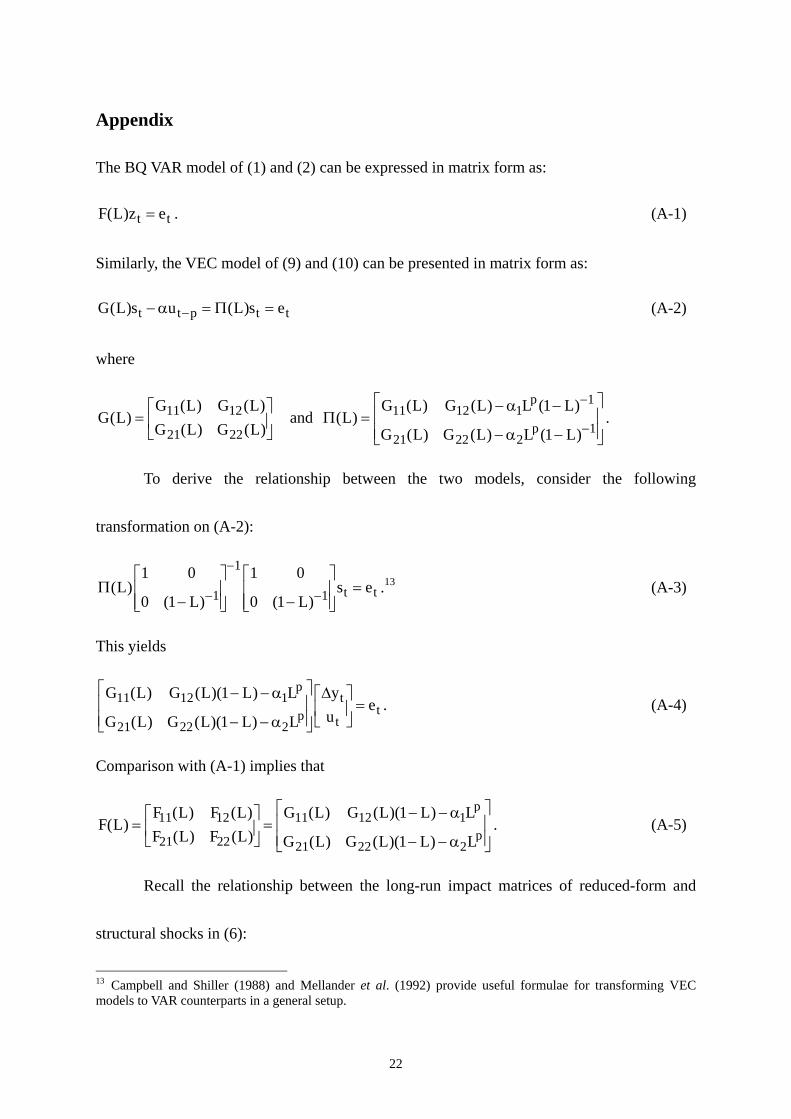
The BQ VAR model of (1) and (2) can be expressed in matrix form as:

t tF(L)z e= . (A-1)

Similarly, the VEC model of (9) and (10) can be presented in matrix form as:

t t p t tG(L)s u (L)s e−− α = Π = (A-2)

where

11 12

21 22

G (L) G (L)G(L)

G (L) G (L)⎡ ⎤

= ⎢ ⎥⎣ ⎦

and p 1

11 12 1p 1

21 22 2

G (L) G (L) L (1 L)(L)

G (L) G (L) L (1 L)

−

−

⎡ ⎤− α −⎢ ⎥Π =⎢ ⎥− α −⎣ ⎦

.

To derive the relationship between the two models, consider the following

transformation on (A-2):

1

t t1 1

1 0 1 0(L) s e

0 (1 L) 0 (1 L)

−

− −

⎡ ⎤ ⎡ ⎤Π =⎢ ⎥ ⎢ ⎥

− −⎢ ⎥ ⎢ ⎥⎣ ⎦ ⎣ ⎦.13 (A-3)

This yields

pt11 12 1

tp t21 22 2

yG (L) G (L)(1 L) Le

uG (L) G (L)(1 L) L

⎡ ⎤ Δ− − α ⎡ ⎤⎢ ⎥ =⎢ ⎥⎢ ⎥ ⎣ ⎦− − α⎣ ⎦

. (A-4)

Comparison with (A-1) implies that

p11 12 11 12 1

p21 22 21 22 2

F (L) F (L) G (L) G (L)(1 L) LF(L)

F (L) F (L) G (L) G (L)(1 L) L

⎡ ⎤− − α⎡ ⎤⎢ ⎥= =⎢ ⎥⎢ ⎥⎣ ⎦ − − α⎣ ⎦

. (A-5)

Recall the relationship between the long-run impact matrices of reduced-form and

structural shocks in (6):

13 Campbell and Shiller (1988) and Mellander et al. (1992) provide useful formulae for transforming VEC models to VAR counterparts in a general setup.

23

0(1) C(1)Γ = Γ , (6)

or, equivalently,

1 1 10(1) ( C(1) )− − −Γ = Γ . (A-6)

Equations (3), (A-1), and (A-5) imply that

11 11

21 2

G (1)C(1) F(1)

G (1)− −α⎡ ⎤

= = ⎢ ⎥−α⎣ ⎦. (A-7)

10−Γ is given in (14) as:

'11

0 1 ' 11

⊥−− −

⎡ ⎤Λ α⎢ ⎥Γ =⎢ ⎥Φ αΩ⎣ ⎦

. (14)

By using (A-7) and (14) with ' 0⊥α α = , it can be shown that

1 1 1 2 11 11 10

1 22 2 12 2 11 1 12 21 2

G (1) 0C(1)

( ) ( ) G (1)⊥ ⊥− − Λ α Λ α −α ∗⎡ ⎤ ⎡ ⎤ ⎡ ⎤

Γ = =⎢ ⎥ ⎢ ⎥ ⎢ ⎥Ξ α Ω −α Ω Ξ α Ω −α Ω −α ∗ ∗⎣ ⎦⎣ ⎦ ⎣ ⎦ (A-8)

where 11(1/ | |) −Ξ = Ω Φ , 11Ω , 22Ω , and 12Ω are the variances of 1te and 2te and their

covariance in Ω , respectively, and ∗ denotes a non-zero element. Because 1 10 C(1)− −Γ is

lower triangular, so is (1)Γ from (A-6). The long-run output neutrality condition is evident.

The lower triangularity of (1)Γ together with uncorrelatedness between AS and AD shocks

in (15) satisfy the assumptions of the BQ model. The BQ model and its cointegrated

representation become equivalent and they generate identical empirical results.

24

References

Astley, M. and T. Yates, 1999, Inflation and real disequilibria. Bank of England Working

Paper No. 103.

Beveridge, S. and C. Nelson, 1981, A new approach to decomposition of economic time

series into permanent and transitory components with particular attention to

measurement of the business cycle, Journal of Monetary Economics 7, 151−174.

Blanchard, O. and D. Quah, 1989, The dynamic effects of aggregate demand and supply

shocks, American Economic Review 79, 655−673.

Blanchard, O. and L. Summers, 1986, Hysteresis and the European unemployment problem,

NBER Macroeconomics Annual, 15−77.

Campbell, J. and G. Mankiw, 1987, Are output fluctuations transitory?, Quarterly Journal of

Economics 102, 857−880.

Campbell, J. and R. Shiller, 1988, Interpreting cointegrated models, Journal of Economic

Dynamics and Controls 12, 505−522.

Cooley, T. and M. Dwyer, 1998, Business cycle analysis without much theory: A look at

structural VARs, Journal of Econometrics 83, 57−88.

Cover, J., W. Enders, and J. Hueng, 2006, Using the aggregate demand-aggregate supply

model to identify structural demand-side and supply-side shocks: Results using a

bivariate VAR, Journal of Money, Credit, and Banking 38, 777−790.

Dolado, J. and J. Jimeno, 1997, The causes of Spanish unemployment: A structural VAR

approach, European Economic Review 41, 1281–1307.

Engle, R. and C. Granger, 1987, Cointegration and error correction: Representation,

estimation and testing, Econometrica 55, 251–276.

Englund, P., A. Vredin, and A. Warne, 1994, Macroeconomic shocks in an open economy: A

common trend representation of Swedish data 1871-1990, in V. Bergström and A.

25

Vredin (eds), Measuring and Interpreting Business Cycles, Clarendon Press, 125−223.

Escribano, A. and D. Pena , 1994, Cointegration and common factors, Journal of Time Series

Analysis 15, 577−586.

Fisher, L. and H-S. Huh, 2007, Permanent-transitory decompositions under weak exogeneity,

Econometric Theory 23, 183−189.

Fisher, L., H-S. Huh, and P. Summers, 2000, Structural identification of permanent shocks in

VEC models: A generalization, Journal of Macroeconomics 22, 53−68.

Fry, R. and A. Pagan, 2005, Some issues in using VARs for macroeconometric research,

Center for Applied Macroeconomic Analysis Working Paper No. 19, Australian

National University.

Giordani, P., 2004, An alternative explanation of the price puzzle, Journal of Monetary

Economics 51, 1271−1296.

Gonzalo, J. and S. Ng, 2001, A systematic framework for analyzing the dynamic effects of

permanent and transitory shocks, Journal of Economic Dynamics and Control 25,

1527−1546.

Jacobs, J. and K. Wallis, 2005, Comparing SVARs and SEMs: Two models of the UK

economy, Journal of Applied Econometrics 20, 209−228.

Johansen, S., 1991, Estimation and hypothesis testing of cointegrating vectors in Gaussian

vector autoregressive models, Econometrica 59, 1551−1580.

Johansen, S. and K. Juselius, 1990, Maximum likelihood estimation and inference on

cointegration: With application to the demand for money, Oxford Bulletin of

Economics and Statistics 52, 169−210.

Keating, J., 2005, Interpreting permanent and transitory shocks to output when aggregate

demand may not be neutral in the long-run, University of Kansas, manuscript,

downloadable from http://www.people.ku.edu/~jkeating.

King, R., C. Plosser, and S. Rebelo, 1988, Production, growth and business cycles: II. New

26

directions, Journal of Monetary Economics 21, 309−341.

King, R., C. Plosser, J. Stock, and M. Watson, 1991, Stochastic trends and economic

fluctuations, American Economic Review 81, 819−840.

Levtchenkova, S., A. Pagan, and J. Robertson, 1996, Shocking stories, Journal of Economic

Surveys 12, 507−532.

Mellander, E., A. Vredin, and A. Warne, 1992, Stochastic trends and economic fluctuations in

a small open economy, Journal of Applied Econometrics 7, 369−394.

Pagan, A. and J. Robertson, 1995, Resolving the liquidity effect, Federal Reserve Bank of St.

Louis Review 77, 33−54.

Pesaran, H. and R. Smith, 1998, Structural analysis of cointegrating VARs, Journal of

Economic Surveys 12, 471−505.

Shiller, R., 1986, Comment, in R. Gordon (ed.), The American Business Cycle: Continuity

and change, University of Chicago Press, 157−158.

Stadler, G., 1986, Real versus monetary business cycle theory and the statistical

characteristics of output fluctuations, Economics Letters 22, 51−54.

27

Table 1: Tests for error-correction coefficients Real output Unemployment

Country 1α t-test 2α t-test

Germany − 0.062 (0.03) 0.04 − 0.005 (0.01) 0.35

Japan − 0.050 (0.14) 0.72 − 0.021 (0.01) 0.03

U.S. 0.048 (0.05) 0.32 − 0.034 (0.01) 0.02 The second column reports the estimate for the error correction coefficient 1α in the output equation (9). Figures in parentheses are the standard errors. The third column reports the marginal significance level (p-value) of t-test statistic for the null hypothesis that 1α is equal to zero. The fourth and fifth columns do the same for the equation of the unemployment rate in (10).

28

Table 2: Forecast error variance decompositions for Germany BQ model BQ-L model

Real output Unemployment Real output Unemployment

Qtrs AS AD AS AD AS AD AS AD

1 54.2 45.8 87.0 13.0 100.0 0.0 19.6 80.4

2 62.0 38.0 87.5 12.5 98.4 1.6 20.2 79.8

4 70.4 29.6 89.8 10.2 95.8 4.2 23.5 76.5

8 78.4 21.6 91.4 8.6 91.5 8.5 25.8 74.2

10 82.2 17.8 90.5 9.5 87.7 12.3 24.5 75.5

20 90.5 9.5 86.5 13.5 76.8 23.2 19.7 80.3

30 93.3 6.7 86.0 14.0 73.4 26.6 18.9 81.1

40 94.8 5.2 85.6 14.4 71.1 28.9 18.5 81.5

50 95.8 4.2 85.5 14.5 69.2 30.8 18.3 81.7

60 96.5 3.5 85.4 14.6 67.7 32.3 18.2 81.8

70 97.1 2.9 85.3 14.7 66.5 33.5 18.1 81.9

80 97.4 2.6 85.3 14.7 65.4 34.6 18.0 82.0

90 97.7 2.3 85.2 14.8 64.5 35.5 18.0 82.0

100 98.0 2.0 85.2 14.8 63.7 36.3 18.0 82.0 The figures are the fractions of the forecast error variance of the series attributable to aggregate supply (AS) and aggregate demand (AD) shocks.

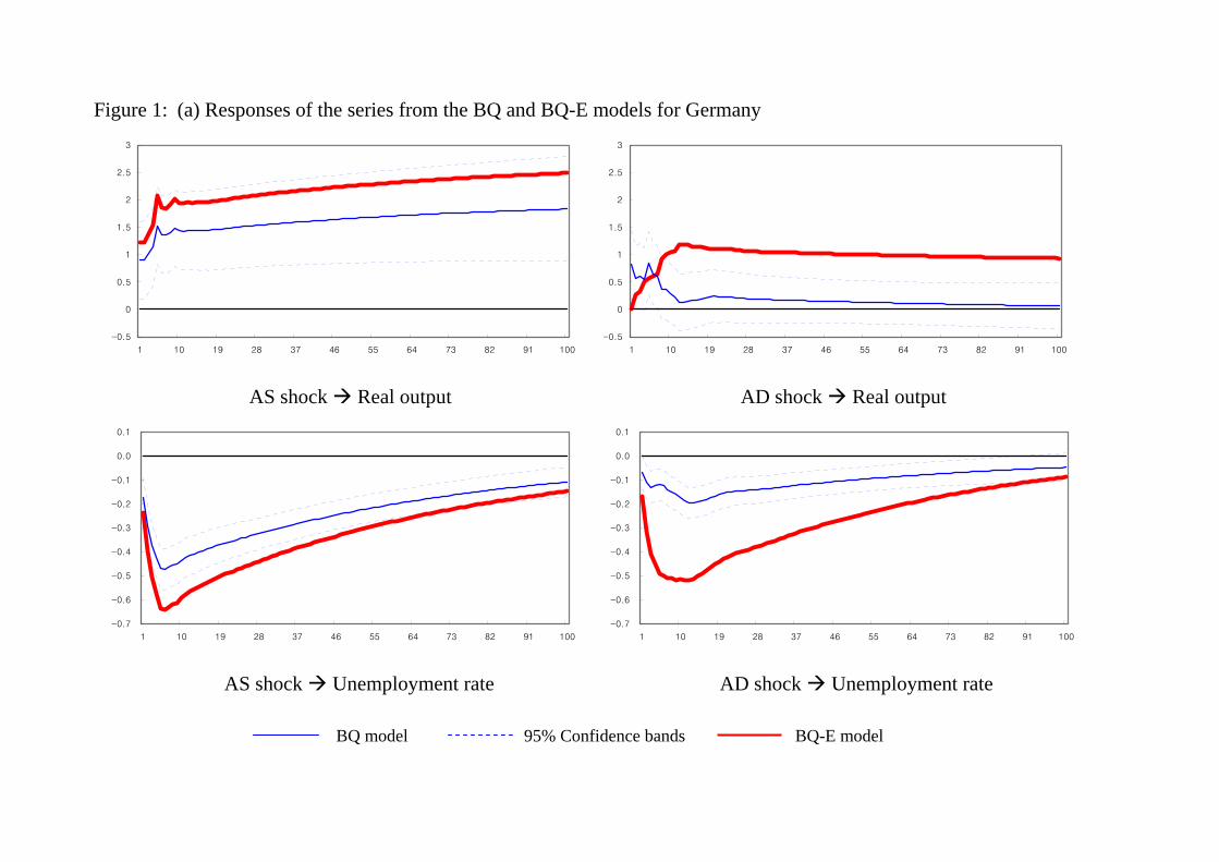
Figure 1: (a) Responses of the series from the BQ and BQ-E models for Germany

-0.5

0

0.5

1

1.5

2

2.5

3

1 10 19 28 37 46 55 64 73 82 91 100

-0.5

0

0.5

1

1.5

2

2.5

3

1 10 19 28 37 46 55 64 73 82 91 100

AS shock Real output AD shock Real output

-0.7

-0.6

-0.5

-0.4

-0.3

-0.2

-0.1

0.0

0.1

1 10 19 28 37 46 55 64 73 82 91 100

-0.7

-0.6

-0.5

-0.4

-0.3

-0.2

-0.1

0.0

0.1

1 10 19 28 37 46 55 64 73 82 91 100

AS shock Unemployment rate AD shock Unemployment rate

BQ model 95% Confidence bands BQ-E model

30

Figure 1: (b) Responses of the series from the BQ and BQ-E models for Japan

-2

-1

0

1

2

3

4

5

6

7

8

1 10 19 28 37 46 55 64 73 82 91 100

-2

-1

0

1

2

3

4

5

6

7

8

1 10 19 28 37 46 55 64 73 82 91 100

AS shock Real output AD shock Real output

-0.20

-0.15

-0.10

-0.05

0.00

0.05

1 10 19 28 37 46 55 64 73 82 91 100

-0.20

-0.15

-0.10

-0.05

0.00

0.05

1 10 19 28 37 46 55 64 73 82 91 100

AS shock Unemployment rate AD shock Unemployment rate

BQ model 95% Confidence bands BQ-E model

31

Figure 1: (c) Responses of the series from the BQ and BQ-E models for the U.S.

-0.3

0

0.3

0.6

0.9

1.2

1.5

1.8

1 10 19 28 37 46 55 64 73 82 91 100

-0.3

0

0.3

0.6

0.9

1.2

1.5

1.8

1 10 19 28 37 46 55 64 73 82 91 100

AS shock Real output AD shock Real output

-0.5

-0.4

-0.3

-0.2

-0.1

0

0.1

1 10 19 28 37 46 55 64 73 82 91 100

-0.5

-0.4

-0.3

-0.2

-0.1

0

0.1

1 10 19 28 37 46 55 64 73 82 91 100

AS shock Unemployment rate AD shock Unemployment rate

BQ model 95% Confidence bands BQ-E model

32

Figure 2: Responses of the series from the BQ, BQ-C, and BQ-L models for Germany

-0.5

0

0.5

1

1.5

2

2.5

3

1 10 19 28 37 46 55 64 73 82 91 100

-0.5

0

0.5

1

1.5

2

2.5

3

1 10 19 28 37 46 55 64 73 82 91 100

AS shock Real output AD shock Real output

-0.7

-0.6

-0.5

-0.4

-0.3

-0.2

-0.1

0.0

0.1

1 10 19 28 37 46 55 64 73 82 91 100

-0.7

-0.6

-0.5

-0.4

-0.3

-0.2

-0.1

0.0

0.1

1 10 19 28 37 46 55 64 73 82 91 100

AS shock Unemployment rate AD shock Unemployment rate

BQ model 95% Confidence bands BQ-C model BQ-L model