Embed Size (px)
Citation preview

1
An Empirical Study of Revenue Management Practices in the Airline Industry
Minho Cho · Ming Fan · Yong-Pin Zhou
Department of Information Systems and Operations Management
Michael G. Foster School of Business University of Washington Seattle, WA 98195-3200
[email protected] · [email protected] · [email protected]
November 15, 2007
Abstract
Revenue management has been successfully implemented in the airline industry since the deregulation in 1978. There have been very few comprehensive, rigorous studies of its practices and impact, however. In this paper we examine how revenue management practices affect airline performances such as load-factor and revenue, and how revenue management practices are implemented in different market structures. Specifically, we use data from the Bureau of Transportation Statistics to empirically examine the pattern of price dispersion in the U.S. airline industry. We also study how operational factors such as capacity, code-share and presence of the hub affect airline pricing, load factor, and revenue. Our results show that these operational factors have significant impacts on price dispersion, load factor and revenue. We use two commonly-used analytical revenue management models to gather insights, and find their predictions largely agree with our empirical findings. Key words: revenue management, airline industry, empirical study

2
1. Introduction
Since the deregulation of airline industry in 1978, revenue management (RM) has gained much
attention as a successful application in the airline industry (Talluri and van Ryzin 2004). Airlines
and other transportation companies view RM systems and related information technologies as
critical determinants of future success (McGill and van Ryzin 1999), and have invested heavily
in such systems. It is commonly believed that the use of RM systems has led to lower fares for
consumers and higher productivity, measured in passenger loads and revenue, for the airlines.
However, there have been few comprehensive, rigorous studies of the practices and impact of
revenue management.
The objective of RM is to sell the right inventory unit to the right consumer, at the right
time, and for the right price (Kimes 1989). The two commonly used techniques are inventory
allocation and dynamic pricing (McGill and van Ryzin 1999). Inventory allocation, or quantity-
based RM, refers to opening and closing predefined booking classes (Philips 2005). Dynamic
pricing, or price-based RM, refers to changing price over time for each fare class. Thus, both
techniques lead to price dispersion. There is an extensive body of research on RM in the
operations management (OM) literature. In order to maintain analytical tractability, OM models
typically focus on a few factors such as booking limit, dynamic pricing, or overbooking (Talluri
and van Ryzin 2004). As such, they do not provide a broad view on the relationships among
various operational factors. There are a number of empirical studies on airline pricing, mainly
from the economics literature (e.g. Borenstein and Rose 1994) that focus on market structure and
regulatory implications such as how competition and market structure affect airline pricing, but
they overlook the effects of some important operational factors such as capacity and code-share
on pricing.

3
Our study aims to link and extend these research streams by using data from the Bureau
of Transportation Statistics (BTS) to empirically examine the relations among markets structure,
airlines’ operational factors, and RM practices. To represent the extent of revenue management
use, we use price dispersion as the metric.
Specifically, our study has two components. First, we examine the effects of airline’s
operational factors and market characteristics on price dispersion. Second, we examine the
effects of price dispersion, along with the operational factors, on the performance of RM
practices. There are multiple metrics to measure the performance of RM. The most important is
revenue. We also use load factor as a performance measure, since it is commonly suggested that
the implementation of RM results in fuller planes (e.g. see Borenstein and Rose 1994).
Our results suggest that airlines’ deliberate RM practice is a major source of price
dispersion. Operational factors such as capacity, code-share and presence of the hub have
significant impacts on price dispersion, load factor, and revenue. One of the interesting results is
that price dispersion tends to increase route level revenue and decrease load factor. Moreover, we
find that capacity tends to increase load factor. To explain these findings, we also analyze two
commonly-used analytical models (quantity-based and price-based respectively). The insights
and predictions generated by these two models largely agree with our empirical findings. To our
knowledge, our paper is among the first to examine how RM practices affect airline
performances such as load-factor and revenue, and how RM practices are implemented in
different market structures.
The rest of the paper is organized as follows. In Section 2, we provide a review of related
literatures. Section 3 describes the datasets and variables. Econometric models and results are
presented in Sections 4 and 5, respectively. In Section 6, we discuss the results and implications.

4
Concluding remarks and future directions are provided in Section 7. Details of the two analytical
RM models can be found in the Appendix.
2. Literature Review
There are two important streams of research on RM: (i) empirical studies on airline price
dispersion in economics, and (ii) analytical RM models in the OM literature.
In the economics literatures, studies have empirically examined the relationship between
airline pricing and various market factors. Borenstein and Rose (1994) find a significant positive
effect of competition on price dispersion in the US domestic airline industry. Hayes and Ross
(1998) find airlines’ price discrimination policies lead to increased price dispersion.
Market power or airport dominance is considered another critical determinant of airline
pricing. Borenstein (1989, 1990) finds that airport dominance enhances a carrier’s ability to
attract passengers and charge higher fares. This may be attributed to biases due to computer
reservation systems, the dominant carrier’s local reputation, control of critical inputs such as
gates and slots, and marketing strategies such as frequent flier plans (Evans and Kessides 1993).
Peteraf and Reed (1994) find that a monopolist’s national market share has a positive effect on
fares and that prices tend to decrease in the number of passengers and route distance.
Ito and Lee (2007) provide a good summary of the US domestic airline alliances. They
find that characteristics of domestic code-share are different from those of international code-
share. Moreover, they find that the average code-share fare is lower than the average fare that is
not code-shared. Bamberger et al. (2004) also find that the price tends to decrease after alliances.
Their findings are similar to those of Park and Zhang (2000), Brueckner and Whalen (2000), and
Brueckner (2001, 2003) who examine international alliances.

5
Most of the OM literature on RM deals with specific policies of revenue maximization.
The quantity-based RM models start with Littlewood’s seminal work (Littlewood 1972,
henceforth referred to as the Littlewood model). The Littlewood model studies how the fixed
total capacity should be allocated between two classes of seats once fares are determined. The
model assumes a fixed number of seats and two independent classes of demand—demand for
full-fare tickets and demand for discount-fare tickets. Discount-fare demand occurs first, and it is
large enough to fill all the allocated seats. The demand for full-fare tickets occurs later and is
random. The model derives the optimal seat protection level for full-fare demand. The analysis
of the problem is similar to that of the classical newsvendor problem in the inventory theory
(Talluri and van Ryzin 2004). The Littlewood model has since been extended to multiple-class
models (Belobaba 1989, Wollmer 1989, Curry 1990, Brumelle and McGill 1993, Robinson
1995) and dynamic models (Lee and Hersh 1993, Feng and Xiao 2001).
For price-based RM models, the seminal work of Gallego and van Ryzin (1994,
henceforth referred to as the GVR model) analyzes the optimal dynamic pricing policy for one
type of product. Gallego and van Ryzin’s dynamic pricing model assumes that consumers arrive
randomly. The optimal price has the following important properties: (i) At any fixed point in
time, the optimal price decreases in the inventory level; conversely, for a given level of inventory
level, the optimal price increases with more time to sell. (ii) For a fixed time and inventory level,
the optimal price increases in the arrival rate. Zhao and Zheng (2000) extend this model to the
case where demand is non-homogeneous. Since consumers are time sensitive, their reservation
price distribution may change over time. For a good review of the current practices in dynamic
pricing, see Elmaghraby and Keskinocak (2003).

6
The Littlewood and GVR models offer important insights that will be used in our
discussion of the empirical findings. Interested readers can find details of the two models in the
Appendix.
OM research on code-share and airline alliance is limited. Shumsky (2006) finds that
low-cost competitors are driving the network airlines to rely on alliances for an increasing
proportion of their traffic. Netessine and Shumsky (2004) analyze a static alliance revenue-
sharing mechanism for a two-leg network based on the expected flow of passengers. Wright et al.
(2006) study a variety of static and dynamic mechanisms to manage RM decisions across
alliances.
3. Data and Variables
3.1. Data
The dataset for this study come from three sources: (i) Airline Origin and Destination Survey, (ii)
Air Carrier Statistics, and (iii) Census of Service Industry. Both (i) and (ii) are from the Bureau
of Transportation Statistics (BTS), and (iii) is from the U.S. Census Bureau. We use the first
quarter of 2005 BTS dataset, which is the latest dataset available at the time of our study.
The Airline Origin and Destination Survey is a 10% sample of airline tickets from the
reporting carriers operated in the US domestic market. All US air carriers which have at least one
percent of domestic market share are required to report the Airline Origin and Destination
Survey quarterly. The dataset contains information such as ticket price, origin, destination, and
other itinerary details.
Air Carrier Statistics contains domestic route level data such as aircraft type, service class
for passengers, number of passengers, available capacity, and number of departures reported by
both US and foreign air carriers.

7
We follow the procedures used in prior studies (e.g. Evans and Kessides 1993, Borenstein
and Rose 1994) to exclude the following data points: (i) non-direct flight tickets, (ii) bulk fares
and fares less than $20, (iii) fares higher than 3.5 times of Standard Industry Fare Level1 (SIFL)
for routes over 500 miles and fares higher than 4 times of SIFL for routes of 500 miles or less,
(iv) routes that have less than three observations, and (v) routes with total number of departures
less than 12 in the quarter, which is approximately less than one departure per week. The reason
to exclude non-direct flight tickets is that those tickets represent significantly different product
types and fares become difficult to compare. We also eliminate unusually high or low fares,
which could be the result of possible data input errors (Hayes and Ross 1998).
The dataset from Census of Service Industry is part of Economic Census managed by U.S.
Census Bureau. We use it to obtain the number of hotel rooms in metropolitan areas in the U.S.
in order to compute the tourism index.
3.2. Variables
We here describe the variables derived from the dataset. The descriptions and descriptive
statistics for all the variables are given in Table 1 and 2 respectively.
Variable GINI is the Gini index of the fares for carrier k with origin i and destination j. It
is a measure of price dispersion, or price inequality. Gini index is a scale invariant measure that
has been applied widely in economics literatures to measure income and price inequality
(Cutright 1967, Borenstein and Rose 1994, Hayes and Ross 1998). It is computed as:
21
2 1n
ll
nGini lXn X n=
+= −∑ (1)
1 The Civil Aeronautics Board established SIFL based upon fares in effect on July 1, 1979. The Department of Transportation provides the SIFL adjustment factor semiannually to aid in its evaluation of carrier pricing. For more details, visit http://www.dot.gov.

8
where lX ( 1,..., l n= ) are the prices in ascending order and X is the average price. Higher
GINI simply indicates higher price dispersion.
LDFACTOR is the load factor, a.k.a. fill rate, for a carrier on a specific route. It is
calculated as the total number of passengers divided by the total number of seats available for
carrier k with origin i and destination j. LDFACTOR measures an airline’s capacity utilization.
REVENUE is the revenue per available seat mile (RASM) for airline k with origin i and
destination j. It can measure the overall effectiveness of an airline RM practice (Philips 2005).
We obtain the values of LDFACTOR and REVENUE from Air Carrier Statistics.
HERFDHL is the Herfindahl index, which is commonly used to measure the degree of
competitiveness in the market. It is calculated as:
2
1HERFDHL=
m
kk
S=
∑ , (2)
where kS is the market share of airline k on a particular route ij, and m is the number of airlines
on that route. Thus, a lower HERFDHL indicates that the route is more competitive, while a
higher HERFDHL represents a less competitive route.
TOURIST is the average tourism index of origin and destination cities. It is computed as
the number of hotel rooms per city population. Higher TOURIST indicates the route is more
tourism oriented.
CAPACITY, CODESHAR, and HUB are airlines’ operation variables. CAPACITY is the
total number of seats provided by a carrier for a route. CODESHAR is the percentage of code-
share tickets out of total number of tickets sold. A ticket is defined as code-share if the operating
carrier is different from the ticketing carrier. Finally, HUB is a dummy variable. It equals one if
either the origin or the destination airport of a particular route is a hub for the airline.

9
Table 1: Definition of the Variables
Variables Definition
GINI Gini index of the fares, which is a measure of price dispersion. Higher GINI indicates a larger price inequality.
REVENUE Revenue per available seat mile (RASM) for an airline on a particular route.
LDFACTOR Load factor, a.k.a. fill rate, for an airline in a particular route. It is the total number of passengers per available seat.
HERFDHL Herfindahl index, which is sum of the square of each airline's market share in a particular route. It is a measure of market competitiveness. Smaller HERFDHL indicates a more competitive route.
HUB Dummy variable. It equals 1 if either origin or destination airport of a particular route is a hub for the airline, 0 otherwise.
TOURIST The average tourism index of origin and destination cities. Tourism index is computed as the number of hotel rooms per city population.
CAPACITY Total number of seats of a carrier for a route.
CODESHAR Percentage of code-share tickets of the total number of tickets sold.
DISTANCE Non-stop distance of a route. It serves as a control variable for the model.
Table 2: Descriptive Statistics
Variables Number of Observations Mean Standard
Dev. Min Max
GINI 3,880 0.24 0.06 0.06 0.46 REVENUE 3,880 0.18 0.12 0.03 1.09 LDFACTOR 3,880 0.69 0.13 0.18 0.97 HERFDHL 3,880 0.66 0.26 0.19 1.00 HUB 3,880 0.42 0.49 0.00 1.00 TOURIST 3,880 0.06 0.05 0.01 0.30 CAPACITY 3,880 37,694 37,524 600 316,915 CODESHAR 3,880 0.30 0.45 0.00 1.00 DISTANCE 3,880 884 660 64 4,962

10
DISTANCE is the non-stop distance for a specific route. It serves as a control variable in
the model.
4. Hypotheses and Models
Prior empirical studies have examined how market structures affect price dispersion. Our dataset
allows us to examine airlines’ RM practices from a broader perspective. We argue that factors
such as demand characteristics, airline alliances, and operation policies should also affect airline
price decisions, and subsequently airline performance. These relations are depicted in Figure 1.
Market Structure
Demand
OperationFactors
Load Factor
Revenue
Pricing
Figure 1: Relationships among Variables
Many RM metrics exist, but the two most important ones are load factor and revenue. We
develop hypotheses linking various factors and RM metrics and those relationships are
summarized in Table 3. We first discuss hypotheses regarding price dispersion in Section 4.1.
Then in Sections 4.2 and 4.3, we analyze how price dispersion and other factors affect load
factors and revenue.

11
Table 3: Summary of Hypotheses
Variables Price Dispersion Load factor Revenue
HERFDHL - + +
HUB + + +
TOURIST - + -
CAPACITY +/- + +
CODESHAR + + +/-
GINI N/A +/- +
LDFACTOR N/A N/A +
4.1. Price Dispersion
A number of factors lead to price dispersion. Prior studies identify two types of price dispersion:
competitive and non-competitive (Borenstein and Rose 1994). The competitive-type price
dispersion happens when airlines set their prices above marginal costs and adjust prices subject
to competitive pressure (Burdett and Judd 1983, Phillips 2005 pp. 58-59). Borenstein and Rose
(1994) find that price dispersion increases with more competition, which supports the
competitive-type price dispersion argument. On the other hand, price dispersion could happen in
non-competitive situations, in which airlines charge different prices for different types of
customers. This type of price dispersion is the direct result of airlines’ price discrimination or
RM practices. Therefore, we expect factors such as presence of hub, demand characters, and
airlines’ operation factors all to affect price dispersion.
We note that competitive and non-competitive price dispersions can co-exist. While an
airline can change price due to the competitive pressure, price dispersion can also be a part of the
airline’s intentional plan to maximize its revenue. Since airlines operate in many markets, price

12
dispersion could result from various strategies and these strategies may vary not only across
markets but also throughout different times (Hayes and Ross 1998).
Following the competitive-type price dispersion argument, we expect price dispersion to
be positively associated with the level of market competition. Since higher Herfindahl indicates
lower level of competition, we expect price dispersion to decrease in HERFDHL.
Prior studies have also found some evidences that airlines have competitive advantages in
attracting customers and increasing fare mark-up at their own hubs (Borenstein 1989). With
higher market power, an airline can implement RM practices more effectively. Thus, following
the non-competitive price dispersion argument, we expect price dispersion to be higher at an
airline’s own hubs.
Demand characters should also affect airlines’ pricing. It is commonly acknowledged in
the RM literature that business travelers have lower price sensitivity but higher valuation of time.
In comparison, leisure passengers are more price-sensitive. The key to RM success is to segment
customers based on their demand characteristics and develop differentiated products and services
(Talluri and van Ryzin 2004). Thus, in more tourism-oriented markets, it is harder for airlines to
achieve product differentiations; so we expect lower price dispersion.
From the operational point of view, capacity and pricing are the two key decision
variables, and they can be jointly optimized when airlines adjust both of them simultaneously.
While pricing adjustment can be made in a tactical way within a short time frame, airlines
usually set capacity ahead of time. For the three-month period we study, it is reasonable to
assume that airlines do not adjust capacity based on pricing decisions.2 How airlines change
2 As an example, in the case of American Airlines, the coefficient of variation of the total monthly capacity for the last 12 months since May 2006 is only 0.041 (from http://www.bts.gov), which indicates that the allocation of capacity is very stable.

13
capacity over a longer time horizon is a subject for future study. With a cross-sectional dataset,
our interest is to explore the effect of capacity on price dispersion.
The Littlewood and the GVR models suggest different effects of capacity on price
dispersion. We analyze both models assuming that capacity is correlated with market demand.
For example, an airline has higher capacity on a route mostly because of higher demand. In the
Littlewood model, price dispersion increases in capacity because with higher capacity and
proportionally higher demand, the risk pooling effect or statistical economy of scale allows an
airline to sell more tickets of both discount and full fares, which results in higher price dispersion
in some ranges. In contrast, in the GVR model, higher capacity brings about two opposite effects
that could affect price dispersion. First, everything else being equal, price dispersion decreases in
capacity. Second, high capacity is usually associated with high demand in practice. Everything
else being equal, high demand results in higher price dispersion. Thus, in the GVR model, the
overall effect of capacity on price dispersion depends on which of the two effects is more
dominant. Our simulation results show that the first, negative effect always dominates. We
provide more detailed analysis of these two models in Section A.3 of the Appendix.
Almost all large airlines in the U.S. have now entered into broad code-share partnerships
(Ito and Lee 2007). Despite its importance, there have been few studies in OM on code-share.
While vertical code-share, which involves inter-airline transfers, helps airlines to extend the
scope of their operation networks, and offer relatively seamless travel experience (Netessine and
Shumsky 2004), horizontal code-share is less understood. When an operating carrier allows other
airlines to market its seats, a possible result is product differentiation (Ito and Lee 2007), which
will result in higher price dispersion.

14
4.2. Load Factor
Load factor is a measure of capacity utilization, and it should be affected by market
characteristics. First, competition is likely to decrease load factor as more carriers compete for
customers in the market. Thus, we expect LDFACTOR to increase in HERFDHL as a higher
HERFDHL indicates lower competition. Second, the presence of hubs will allow an airline to
attract more customers. More direct flights, convenient schedules and terminal locations are
some of the benefits for a hub, which can drive up the demand and improve capacity utilization.
Further, we expect high-tourism markets will increase load factor because of relatively
higher demand in those markets. In addition, leisure travelers are more price-sensitive and tend
to book early. If the full-fare demand comprises a smaller proportion of the total demand, we
conjecture, following the Littlewood model, that fewer seats need to be protected for full fare
demand. This reduces the probability of unsold seats and improves load factor.
On a given route, we expect airlines with higher capacity to achieve higher load factor. It
may sound counter-intuitive at first glance. However, higher capacity usually correlates with
higher demand, and because of risk pooling, a system with higher demand and proportionally
higher capacity usually performs better. As a result, fewer seats go unsold and load factor rises.
An analogy is that in supply chains, various forms of risk pooling are used to reduce lost sale
ratio (Cachon and Terwiesch 2006). Numerical results from the Littlewood and GVR models in
Section A.4 in the Appendix clearly demonstrate the risk-pooling effect.
An airline will be able to expand its marketing and operation network through alliances
with other airlines. Thus we expect code-share to increase an airline’s capacity utilization, hence
the load factor.

15
The relationship between price dispersion and load factor is quite intriguing. Some
believe that RM should allow airlines to “fill the plane” as mush as possible (Borenstein and
Rose 1994, Eblen 1996). Thus, if we use price dispersion as an indicator of how extensively RM
is employed, load factor should be positively related with price dispersion. A competing view is
that the ultimate goal of RM is to maximize revenue, which sometimes can be achieved by
selling fewer tickets at higher prices. This may result in higher price dispersion, but lower load
factor. We will test these competing hypotheses in Section 5. The intuition we are able to gather
from both Littlewood and GVR models suggests that load factor should decrease in price
dispersion. In the Littlewood model, as the fare difference increases, the airline will optimally
protect more seats for the high-fare demand, thus increasing the expected number of unsold seats
and lowering the load factor. In the GVR model, the simulation results show that load factor is
decreasing in price dispersion which indicates that the maximum revenue can be achieved with
fewer seats sold. (For details, see Appendix A.6). It will be interesting to see whether empirical
data are consistent with the analytical model predictions.
4.3. Revenue
Revenue per available seat mile (REVENUE) is one of the most important metrics to measure
the overall effectiveness of RM. It can also be used to compare the performance of different
airlines (Phillips 2005). We assume REVENUE to be a function of market structure, demand
characters, and operation factors.
Market structure factors such as competition, presence of hubs, and tourism should have
significant impact on airlines’ performances. As competition tends to lower prices, we expect
that more competition leads to lower REVENUE. On the routes connected to the hubs, the airline
is likely to have higher revenue because it has stronger market power in attracting customers and

16
marking up prices. We also expect REVENUE to be lower in high tourism markets since tourists
are more price sensitive than business travelers, and allow for less price discrimination.
There are a few reasons that REVENUE (recall that it represents revenue per available
seat mile) should be positively correlated with capacity. First, higher capacity usually indicates
market power or airport dominance, which tends to increase fare mark-up (Borenstein 1989).
Second, as argued before, higher capacity usually correlates with higher demand in a market, and
the risk pooling effect allows the airline to improve the overall efficiency of the system. In the
Littlewood model it is obvious that the expected revenue increases in capacity since both
discount- and full-price are predetermined, so increasing sales of two classes due to risk-pooling
result in higher revenue. When we assume that the arrival rate is proportional to the capacity, the
GVR model also predicts that revenue per seat increases in capacity. More details can be found
in Appendix A.5.
The effect of code-share on revenue is somewhat mixed. Empirical studies find that code-
share lowers average fare (Ito and Lee 2007). On the other hand, code-share could increase load
factor as discussed earlier, which has a positive effect on revenue. It will be interesting to
examine which effect dominates the other.
We take the view that price dispersion in the airline industry is mainly due to RM
practices in order to increase revenue. Therefore, we expect price dispersion to have a positive
effect on the carrier’s revenue.
Finally, everything being equal, fuller plane means higher revenue per seat. Thus, we
expect REVENUE to increase in load factor.

17
4.4. Model Specifications
We first discuss the econometric model for price dispersion. The model is similar to those in
Borenstein and Rose (1994) and Hayes and Ross (1998). Each observation in our dataset
corresponds to a single airline k operating between origin i and destination airports j. The price
dispersion model is as follows:
0 1 2 3 4
5 6
ln( ) ln( ) ln( ) ln( )
ln( ) ln( ) ,ijk ij ijk ij ijk
ijk ij k k ij ijk
GINI HERFDHL HUB TOURIST CAPACITY
CODESHAR DISTANCE d
α α α α α
α α δ μ ε
= +
+ + + +
+ + +
+ (3)
where kd is the airline dummy and the error term ijμ captures the unobservable route effects
such as demand, cost, and weather pattern that are constant for all airlines for a specific route.
The term ijkε is the random error. All the definitions of the variables can be found in Table 2.
This log-log model provides estimations in constant elasticity (Greene 2003). Therefore, we can
interpret 1α , for example, as the estimated elasticity of price dispersion (GINI) with respect to
the Herfindahl index. It implies that a 1% change in route level Herfindahl index will cause 1α
percent change in GINI index. As discussed earlier, capacity within a three-month period is quite
stable and we do not expect pricing decisions directly affect capacity level.
Similarly, the load factor model is as follows:
0 1 2 3
4 5 6
7
ln( ) ln( ) ln( )
ln( ) ln( ) ln( )
ln( )
ijk ij ijk ij
ijk ijk ijk
ij k k ij ijk
LDFACTOR HERFDHL HUB TOURIST
CAPACITY CODESHAR GINI
DISTANCE d
β β β β
β β β
β η μ ε
=
+ + +
+ + +
+ + +
+
(4)
where kd is airline dummy. The error term has two components: the route level error ijμ and the
random error ijkε .
We specify the revenue model as follows:

18
0 1 2 3
4 5 6
7 8
ln( ) ln( ) ln( )
ln( ) ln( ) ln( )
ln( ) ln( )
ijk ij ijk ij
ijk ijk ijk
ijk ij k k ij ijk
REVENUE HERFDHL HUB TOURIST
CAPACITY CODESHAR GINI
LDFACTOR DISTANCE d
γ γ γ γ
γ γ γ
γ γ λ μ ε
=
+ + +
+ + + +
+ + +
+
(5)
where kd is airline dummy. The error term has two components: the route level error ijμ and the
random error ijkε .
The above models can be estimated using ordinary least square (OLS) or random effects
models. The OLS model, which does not account for the route effects, can result in biased
estimates because of omitted variables bias (Wooldridge 2002). The random effects model
assumes that there is no endogeneity of the independent variables. However, we recognize
potential endogeneities in both Equations (4) and (5). For example, price dispersion (GINI) and
load factor (LDFACTOR) could be correlated with the route level error term. Thus, we use the
Hausman-Taylor (HT) model (Hausman and Taylor 1981, Greene 2003), which uses a two step
instrument variable (IV) method to provide consistent estimation of the coefficients. This
specification assumes that GINI in Equation (4) and both GINI and LDFACTOR in Equation (5)
are endogenous and can be jointly determined.
5. Results
We test for multi-collinearity among the independent variables by calculating the variance
inflation factor (VIF) for all the independent variables. All of the VIF-values are below the
threshold of 10. Consequently, multi-collinearity should not be a problem in our specifications
(Besley et al. 1980).
We follow the procedure suggested by Baltagi et al. (2003) and Greene (2003) to test
model specifications. We first confirm that the route effects ( ijμ ) are significant. We use
Lagrange multiplier (LM) test for the random effects model based on the OLS residuals (Green
19
2003). The LM statistic are 351.37 for Equation (3), 99.91 for Equation (4), and 732.71 for
Equation (5), far exceeding 21,0.01 6.63χ = , which is the 99% critical value for chi-squared with
one degree of freedom. This indicates that route effects are significant and OLS models are not
appropriate. We next test whether there are endogeneities in the models. We use the Hasuman
test (Greene 2003) and the test statistic for (4) is 265.07, which exceeds 222;0.01χ =40.29. The test
statistic for Equation (5) is 1276.99, much higher than 223;0.01χ =41.64 as well. The test results
suggest that route error terms are correlated with other independent variables and, therefore, a
HT specification is appropriate for these three models.
5.1. Price Dispersion Model
Table 4 provides the estimated coefficients of the price dispersion model. Along with the HT
results, we also provide results from the OLS and random effects models. As we can see, the
results are quite robust to different specifications. The sign of HERFDHL is negative, indicating
that price dispersion increases in competition, consistent with prior studies (Borenstein and Rose,
1994) and our hypothesis. Note, however, that HERFDHL is only significant (p<0.1) in the HT
model. On the other hand, we find the effect of HUB is highly significant (p<0.01), indicating
that airlines have higher price dispersions at their own hubs, which supports the theory of non-
competitive price dispersion. Even though the level of tourism in a market has a positive impact
on price dispersion, the effect is not significant in the HT model.
We find that operation factors such as CAPACITY and CODESHAR are highly
significant in affecting price dispersion. First, a carrier’s capacity has a positive effect on price
dispersion (p<0.01), supporting the hypothesis of peak-load pricing. Second, code-share also has
a highly significant positive effect (p<0.01) on price dispersion. This confirms our observation in
Figure 2 and that in McAfee and te Velde (2007). Finally, the control variable of DISTANCE is

20
also positively associated with price dispersion, suggesting routes that have longer flight distance
tend to have higher price dispersion.
Table 4: Estimated Coefficients for the Price Dispersion Model
Dependent variable: ln(GINI) OLS Random Effects HT IV
Intercept -2.213*** -2.199*** -1.952*** (0.074) (0.069) (0.096) ln(HERFDHL) -0.011 -0.014 -0.025* (0.008) (0.010) (0.015) HUB 0.080*** 0.081*** 0.064*** (0.016) (0.014) (0.014) ln(TOURIST) -0.025*** -0.022*** -0.001 (0.006) (0.007) (0.009) ln(CAPACITY) 0.025*** 0.029*** 0.031*** (0.004) (0.004) (0.004) ln(CODESHAR) 0.008*** 0.009*** 0.010*** (0.002) (0.002) (0.002) ln(DISTANCE) 0.067*** 0.065*** 0.039*** (0.005) (0.006) (0.009) R2 0.432 0.426
Notes: N = 3,880. Regressions also include 18 airline dummies.
* p <0.1; ** p < 0.05; *** p < 0.01.
5.2. Load Factor Model
From results in Table 5, we see that the effect of market competition (HERFDHL) on load factor
is not significant. HUB has a significantly positive effect on load factor (p<0.01). It is consistent
with prior studies (Borenstein 1991) that a market dominant airline has a significant advantage in
attracting customers and marking up prices. The effect of TOURIST is positive and significant
(p<0.01), supporting our conjecture that high-tourism markets tend to increase sales, which helps
improve airlines capacity utilization.

21
Operational factors play important roles in affecting carriers’ capacity utilization as well.
Capacity has a significant positive effect on load factor (p<0.01), supporting the risk pooling
argument. A more detailed discussion using Littlwood’s model is given in Appendix. The sign of
code-share effect on load factor is positive, but it is not significant in the HT model.
Finally, the results show that GINI has a negative effect on LDFACTOR (p<0.05),
suggesting higher price dispersion tends to reduce capacity utilization. This contradicts the
popular belief that RM practices “fill the planes,” but is not surprising because the goal of RM is
to maximize revenue, not load factor (Talluri and van Ryzin 2004).
Table 5: Estimated Coefficients for the Load factor Model
Dependent variable: ln(LDFACTOR) OLS Random Effects HT IV
Intercept -1.431*** -1.492*** -1.815*** (0.068) (0.069) (0.103) ln(HERFDHL) 0.008 0.012 0.005 (0.007) (0.008) (0.013) HUB 0.039*** 0.028** 0.056*** (0.013) (0.013) (0.013) ln(TOURIST) 0.057*** 0.058*** 0.033*** (0.005) (0.005) (0.007) ln(CAPACITY) 0.036*** 0.039*** 0.037*** (0.003) (0.003) (0.004) ln(CODESHAR) 0.005** 0.004** 0.003 (0.002) (0.002) (0.002) ln(GINI) -0.083*** -0.081*** -0.055** (0.013) (0.014) (0.026) ln(DISTANCE) 0.113*** 0.119*** 0.155*** (0.004) (0.005) (0.008) R2 0.328 0.323
Notes: N = 3,880. Regressions also include 18 airline dummies.
* p <0.1; ** p < 0.05; *** p < 0.01.

22
5.3. Revenue Model
From results in Table 6, we see that the Herfindahl index has a positive effect on revenue
(p<0.01), suggesting that higher market competition leads to lower revenue. This result is
consistent with the effect of HUB, which also has a significant positive effect on revenue
(p<0.01). The effect of tourism, however, is not significant.
Table 6: Estimated Coefficients for the Revenue Model
Dependent variable: ln(REVENUE) OLS Random Effects HT IV
Intercept 3.758*** 3.515*** 3.754*** (0.088) (0.078) (0.102) ln(HERFDHL) 0.100*** 0.083*** 0.091*** (0.008) (0.010) (0.016) HUB 0.159*** 0.127*** 0.086*** (0.016) (0.012) (0.011) ln(TOURIST) -0.013** -0.016** 0.008 (0.006) (0.007) (0.009) ln(CAPACITY) -0.015*** 0.006* 0.0190*** (0.004) (0.003) (0.003) ln(CODESHAR) 0.005** 0.004** 0.004** (0.002) (0.002) (0.002) ln(GINI) 0.291*** 0.241*** 0.190** (0.016) (0.015) (0.019) ln(LDFACTOR) 0.861*** 0.955*** 1.026*** (0.020) (0.017) (0.017) ln(DISTANCE) -0.736*** -0.738*** -0.785*** (0.006) (0.006) (0.010) R2 0.884 0.875
Notes: N = 3,880. Regressions also include 18 airline dummies.
* p <0.1; ** p < 0.05; *** p < 0.01.
The effect of capacity on revenue is highly significant (p<0.01) and positive. Even
though the coefficient is negative in the OLS model, the HT is the more appropriate model. The

23
effect of code-share on revenue is also positive and significant (p<0.05). This is not surprising
and explains the prevalence of airline alliances.
The results show that price dispersion (GINI) has a significant positive effect on revenue
(p<0.05). Thus, we have empirical proof that RM practices do achieve its goal of increasing
airline revenue. Further, load factor is highly significant in affecting revenue (p<0.01).
Interestingly, we find REVENUE tends to be lower in routes with longer flight distance.
Note that, since REVENUE measures the revenue per available seat mile, it is already
normalized by flight distance.
6. Discussion and Alternative Explanation
6.1 Sources of Price Dispersion
As we have discussed earlier, the sources of price dispersion can be categorized as either
competitive or non-competitive. Consistent with prior literature (Borenstein and Rose 1994), our
empirical analysis reveals that higher market competition is associated with higher price
dispersion, suggesting that airlines adjust their prices subject to competitive pressure. However,
as shown in Table 4, the marginal effect of competition on price dispersion is relatively low
compared to other factors.
Operational factors such as the presence of hub, capacity and code-share belong to the
source of non-competitive price dispersion. First of all, we can see the presence of hub has a
significant effect on price dispersion, suggesting that airlines usually implement RM practices
more effectively at their hubs where they have dominant market power.
Second, we find capacity is positively associated with price dispersion. The Littlewood
and GVR models suggest contrasting relations between price dispersion and capacity. So our

24
result that capacity positively impact price dispersion is interesting and worth more in-depth
discussion. We do that in Section 6.2.
Further, the result that code-share has a positive impact on price dispersion is also worth
more in-depth discussion, which we will do in Section 6.3.
Overall, our empirical results provide strong evidence for the presence of non-
competitive price dispersion. It implies airlines’ deliberate RM practice is a major source of price
dispersion. Factors such as the presence of hub, capacity level, and code-share agreement affect
an airline’s ability to attract different types of customers. Price dispersion may increase as
airlines can effectively segment demand and charge diverse prices to its customers.
It is somewhat surprising that the characteristic of demand measured by tourism index
have positive effect on price dispersion. Since it is not significant in the HT model, we consider
this finding inconclusive.
6.2 Impact of Capacity
In Section 4.1, we argue that Littlewood model suggests a positive relation between
capacity and price dispersion, while the GVR model suggests the opposite. (For details, see
Appendix A.1.) These are not necessarily contradictory. In practice, airlines’ RM systems
incorporate elements of both models: airlines first define broad fare classes and allocate capacity
among them (as in the Littlewood model). Then, in real time, airlines fine tune the price of each
fare class (as in the GVR model). From this perspective, price dispersion in the Littlewood
model is the result of price disparity and fare allocation between different fare classes, while
price dispersion in the GVR model represents price variation within a single fare class. Our
empirical analysis finds a positive impact of capacity on price dispersion. One explanation is that

25
the effect of inter-class price difference (the Littlewood model) dominates that of intra-class
price changes (the GVR model).
An alternative explanation for the positive relationship between capacity and price
dispersion is peak-load pricing (Bergstrom and MacKie-Mason 1991). When an airline has a
large capacity, multiple flights could be distributed at different high- and low-demand times
during a day or a week. Airlines can achieve efficient capacity utilization by pricing differently
in peak and off-peak periods. Thus, a large capacity on a route could also lead to higher price
dispersion on that route. Although peak-load pricing receives little attention in OM literature, it
serves as an important RM tool (Talluri and van Ryzin 2004).
It is also interesting that our results are largely consistent with the predictions from both
Littlewood and GVR models on the relationship between capacity and load factor. A system of
high capacity usually provides better performance because of risk pooling effects. The critical
assumption of the result is that high capacity is due to high demand. If this assumption is violated
and there are extra capacities than demand, load factor may decrease as capacity increases. Thus,
our results imply that, during the time of study, the airlines operated without much extra capacity,
which is consistent with many airlines practices on capacity control (Carpenter 2007).
6.3 Code-Share and Airline Alliance
Our results show that code-share increases price dispersion, consistent with the view that the
effect of code-share is largely product differentiation (Ito and Lee 2007), which could lead to
different prices. We have collected fare data on code-share flights. An example is shown in
Figure 2. The two flights between Los Angeles and Chicago are offered by American and Alaska
Airlines respectively, but they are code-shared. Since the two flights in effect use the same
aircraft and offer the same schedule and service, they can be considered “identical” products.

26
Yet, prices on these two flights vary significantly. McAfee and te Velde (2007) notes the same
phenomenon. In our view, passengers view these two flights differently. For example, passengers
are more inclined to buy tickets from the airlines with which they have frequent flyer miles. In
addition, search costs could prohibit consumers from being fully aware of the availability of
perfectly substitutable products at a lower price.
R ound trip LA X-O R D -LA X
0
200
400
600
800
1000
1200
0 5 10 15 20 25 30
Tim e (D ay)
Price ($)
A m erican (O perating C arrier A laska
D eparture
Figure 2: Price Dispersion of Code-Shared Flights
Although airlines can do a better job coordinating their code-share agreements (Shumsky
2006, Wright et al. 2006), our empirical results show that existing code-share agreements already
tend to lead to higher revenue per available seat mile. Note that because we are unable to split
the total revenue between the operating and marketing airlines, our results only suggest that
code-share could lead to higher overall revenue. The issue to efficiently allocate the total surplus
to individual airline in the code-share alliance is indeed an important research problem.
6.4 Effects of Price Dispersion
One of the interesting results is that price dispersion has a negative effect on load factor, but a
positive effect on revenue. These results further demonstrate the goal of RM is to maximize
revenue, even if it comes at the expense of lower load factors. When situation calls for larger

27
price dispersion, airlines tend to allocate more seat capacity to future higher-fare passengers,
through more protected seats or high-priced tickets. Although this may lead to less full planes, it
is still worthwhile when those on board are paying higher prices for their seats and the overall
revenue is higher.
7. Conclusions
We use the data from BTS to empirically examine the RM practices in the airline
industry. Our study expands the existing empirical research on airline pricing by accounting for
important operational factors such as hub, code-share, and capacity. Results show that these
factors indeed have significant effects on price dispersion, load factor, and revenue. Because our
model includes important factors such as market structure and demand characteristics, our
empirical study also extends the analytical RM models. Moreover, we are able to use the
insights generated by the analytical models to get a deeper understanding of the empirical results.
Overall, our study confirms the belief that RM is an important contributor to airline
performances. Moreover, operational factors such as capacity, code-share, and hub presence
have significant impact on price dispersion, load factor, and revenue. These have strategic
implications for the airlines. For example, the positive effect of code-share on revenue suggests
that airlines should consider using code-share as a strategic tool to improve performances.
Another important observation is that price dispersion tends to increase the revenue while
it tends to decrease load factor. This is confirmed by the analytical insights generated by the
Littlewood and GVR models. It underlies the important concept that the ultimate goal of RM is
to maximize revenue, even if it comes at the expense of less full planes. This also helps to dispel
the misbelief that RM aims to fill as many seats as possible.

28
Although our model offers a comprehensive view of the airlines’ RM practices and their
impact on airline performances, many of its observations cannot be fully explained by the
existing analytical models. For example, code-share agreements tend to increase price dispersion
and revenue, but the mechanism through which these are achieved is unknown. It is an
interesting topic for future research.
References
Bamberger, G.E., D.W. Carlton and L.R. Neumann. 2004. An empirical investigation of the
competitive effects of domestic airline alliances. Journal of Law and Economics XLVII,
195-222.
Baltagi, B., G. Bresson and A. Pirotte. 2003. Fixed effects, random effects or Hausman-Taylor?
A pretest estimator. Economics Letters 79 (3) 361-369.
Belobaba, P. 1989. Application of a probabilistic decision model to airline seat inventory control.
Operations Research 37, 183-197.
Belsley, D.A., E. Kuh and R.E. Welsch. 1980. Regression Diagnostics: Identifying Influential
Data and Sources of Collinearity. John Wiley & Sons, New York, N.Y.
Bergstrom, T. and J. MacKie-Mason. 1991. Some simple analytics of peak-load pricing. Rand
Journal of Economics 22, 241-249.
Borenstein, S. 1989. Hubs and High Fares: Dominance and Market Power in the U.S. Rand
Journal of Economics 20 (3), 344-365.
Borenstein, S. 1991. The Dominant-firm advantage in Multiproduct Industries: Evidence from
the U.S. Airlines. The Quarterly Journal of Economics 106 (4), 1237-1266.

29
Borenstein, S. and N.L. Rose. 1994. Competition and Price Dispersion in the US Airline
Industry. The Journal of Political Economy 102 (4), 653-683.
Brueckner, J and T. Whalen. 2000. The price effects of international airline alliances. Journal of
Law and Economics 43, 503-545.
Brumelle, S.L. and J.I. McGill. 1993. Airline seat allocation with multiple nested classes.
Operations Research 41, 127-137.
Burdett, K. and K.L. Judd . 1983. Equilibrium price dispersion. Econometrica 51(4), 955-969.
Cachon, G. and C. Terwiesch. 2006. Matching supply with demand. McGraw-Hill/Irwin.
Carpenter, D. 2007. Fuller planes pay off for UAL bottom line. The Grand Rapids Press, July 25.
Curry, R.E. 1990. Optimum seat allocation with fare classes nested by origins and destinations.
Transportation Science 24, 193-203.
Dresner, M and R. Windle. 1992. Airport dominance and yields in the U.S. airline industry.
Logistics and Transportation Review 28 (4), 319-339.
Eblen, T. 1996. The grounding of Valuejet Airlines must try to fill all seats, charge the highest
possible fare. The Atlanta Journal-Constitution, June 23.
Elmaghraby, W. and P. Keskinocak. 2003. Dynamic pricing in the presence of inventory
considerations: research overview, current practices, and future directions. Management
Science 49 (10), 1287-1309.
Evans, W. and I. Kessides. 1993. Localized market power in the U.S. airline industry. The
Review of Economics and Statistics 75, 66-75.
Gallego, G. and G. van Ryzin. 1994. Optimal dynamic pricing of inventories with stochastic
demand over finite horizon. Management Science 40, 999-1020.
Greene, W.H. 2003. Econometric Analysis. Prentice Hall, Upper Saddle River, N.J.

30
Hayes, K. and L.B. Ross. 1998. Is price dispersion the result of careful planning or competitive
forces? Review of Industrial Organization 13, 523-541.
Ito, H. and D. Lee. 2007. Domestic codesharing, alliances and airfares in the US airline industry.
Forthcoming in Journal of Law and Economics.
Kimes, S.E. 1989. Yield management: a tool for capacity-constrained service firm. Journal of
Operations Management 8, 348-363.
Lee, T.C. and M. Hersh. 1993. A model for dynamic airline seat inventory control with multiple
seat bookings. Transportation Science 27, 252-265.
Littlewood, K. 1972. Forecasting and control of passengers. 12th AGIFORS Symposium
Proceedings. Nathanya, Israel, 95–128.
McAfee, R. and V. te Velde. 2007. Dynamic pricing within the airline industry. Working Paper,
California Institute of Technology. (Available at
http://vita.mcafee.cc/PDF/DynamicPriceDiscrimination.pdf.)
McGill, J. and G. van Ryzin. 1999. Revenue management: Research Overview and Prospects.
Transportation Science 33, 233-256.
Netessine, S. and R. Shumsky. 2004. Revenue Management Games: Horizontal and Vertical
Competition. Management Science. 51 (5) 813-831.
Peteraf, M.A. and R. Reed. 1994. Pricing and performance in monopoly airline markets. Journal
of Law and Economics 37 (1), 193-213.
Robinson, L.W. 1995. Optimal and approximate control policies for airline booking with
sequential non-monotonic fare classes. Operations Research, 43, 252-263.
Rothman, A. 2006 Sep. 1. Air France-KLM raises profit forecast for 2006 MARKETPLACE by
Bloomberg. International Herald Tribune, page 13.

31
Shumsky, R. 2006. The Southwest Effect, Airline Alliances, and Revenue Management. Journal
of Revenue and Pricing Management 5(1), 83-89.
Talluri, K. and G. van Ryzin. 2004. The theory and practice of revenue management. Kluwer
Academic Puslishers.
Windle, R. and M. Dresner. 1993. Competition at “Duopoly” Airline Hubs in the US.
Transportation Journal 33 (2), 22-30.
Wollmer, R.D. 1989. An airline seat management model for a single flight leg route when lower
fare classes book first. Operations Research 40, 26-37.
Wright, C.P., H. Groenevelt, and R. Shumsky. 2006. Dynamic Revenue Management in Airline
Alliances, working paper.
Zhao, W., and Y. Zheng. 2000. Optimal dynamic pricing for perishable assets with
nonhomogeneous demand. Management Science 46, 375-388.

32
Appendix: Quantity-Based and Price-Based Revenue Management Models
First, we briefly review two fundamental models of quantity-based and price-based RM: the
Littlewood model and the GVR model. These two models provide the framework of our
discussion on some interesting findings in our empirical study.
A.1. Littlewood Two-Class Seat Allocation Model The Littlewood model provides useful insights about how the fixed total capacity should be
allocated between two classes of seats once fares are determined. In this section, we review its
assumptions, notations, and basic results. The model assumes: (i) there are a fixed number of n
seats, (ii) α∈(0,1) is a discount factor such that the full fare is p, and the discount fare is αp, (iii)
there are two independent classes of demand: demand for full-fare tickets and demand for
discount-fare tickets, (iv) discount-fare demand occurs first, and it is large enough to fill all the
seats allocated, (v) demand for full-fare tickets is random but its distribution is known, and (vi)
there are no cancellations or overbooking. The results for general distribution functions can be
derived, but we assume the demand for full-fare tickets to be normally distributed with mean μ
and standard deviationσ . Therefore, we use the standard notation φ and Φ denote, respectively,
the probability distribution function and the cumulative distribution function.
Optimal Protection Level of q: The optimal protection level, at which the expected revenue is
maximized, can be derived as q zμ σ= + , where 1(1 )z α−= Φ − .
Price Dispersion of Gini: The standard definition of Gini is:
21
2 1n
ll
nGini lXn X n=
+= −∑ (A1)

33
where lX ( 1,..., l n= ) are the prices in ascending order and X is the average price. In the
context of the Littlewood model, let H be the (random) number of full-fare ticket sales, and L=n-
q the (fixed) number of discount-fare ticket sales, then (A1) can be simplified to
* (1 )( )( )( )
L HGini HH L L H
αα−
=+ +
. (A2)
Thus, we can find the expected Gini as:
1[ ] ( ) ( ) 1q H qE Gini Gini H dx Gini qμ μφ
σ σ σ−∞
− ⎡ − ⎤⎛ ⎞ ⎛ ⎞= + − Φ⎜ ⎟ ⎜ ⎟⎢ ⎥⎝ ⎠ ⎝ ⎠⎣ ⎦∫ . (A3)
Expected Sales and Load factor: When q seats are protected for the full-fare demand, the
expected loss sales of full-fare demand is ( )L zσ , where ( ) ( ) (1 ( ))L z z z zφ= − − Φ is the standard
normal loss function (Cachon and Terwiesch 2006). Therefore, the expected number of full-fare
tickets sold is ( )L zμ σ− . Because L= n q− , the expected total ticket sales is:
( )n q L zμ σ− + − . (A4)
Then, the expected load factor can be derived as:
( )( )( ) n z L zn q L zn n
σμ σ − +− + −= . (A5)
Numerical Results: Assuming that both the average ( )μ and the variance 2( )σ of full–fare
demand are linearly increasing in capacity, the numerical results of the Littlewood model show:
(i) price dispersion increases in capacity,
(ii) load factor increases in capacity, and
(iii) revenue increases in capacity.
When we fix the discount fare and vary the full fare, assuming that both the average ( )μ and the
variance 2( )σ of full–fare demand are linearly decreasing in the full fare, we find
34
(iv) load factor first decreases and then increases in price dispersion.
In other words, the relationship is U-shaped. We will discuss these results in more details in
Sections A.3 – A.6, correspondingly.
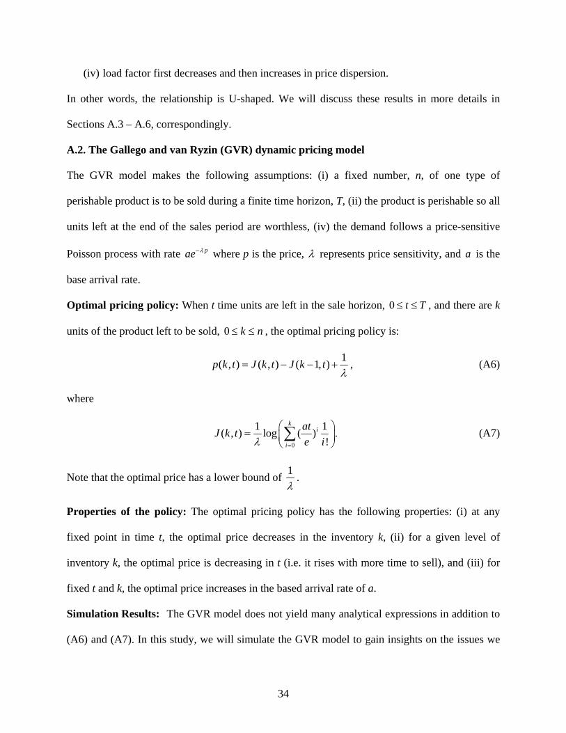
A.2. The Gallego and van Ryzin (GVR) dynamic pricing model
The GVR model makes the following assumptions: (i) a fixed number, n, of one type of
perishable product is to be sold during a finite time horizon, T, (ii) the product is perishable so all
units left at the end of the sales period are worthless, (iv) the demand follows a price-sensitive
Poisson process with rate pae λ− where p is the price, λ represents price sensitivity, and a is the
base arrival rate.
Optimal pricing policy: When t time units are left in the sale horizon, 0 t T≤ ≤ , and there are k
units of the product left to be sold, 0 k n≤ ≤ , the optimal pricing policy is:
1( , ) ( , ) ( 1, )p k t J k t J k tλ
= − − + , (A6)
where
0
1 1( , ) log ( ) .!
ki
i
atJ k te iλ =
⎛ ⎞= ⎜ ⎟⎝ ⎠∑ (A7)
Note that the optimal price has a lower bound of 1λ
.
Properties of the policy: The optimal pricing policy has the following properties: (i) at any
fixed point in time t, the optimal price decreases in the inventory k, (ii) for a given level of
inventory k, the optimal price is decreasing in t (i.e. it rises with more time to sell), and (iii) for
fixed t and k, the optimal price increases in the based arrival rate of a.
Simulation Results: The GVR model does not yield many analytical expressions in addition to
(A6) and (A7). In this study, we will simulate the GVR model to gain insights on the issues we

35
are interested in. Assuming that the base arrival rate ( a ) is linearly increasing in the capacity (n),
the simulation results suggest the following:
(i) price dispersion decreases in capacity,
(ii) load factor increases in capacity,
(iii) revenue per seat is increasing in capacity, and
(iv) load factor decreases in price dispersion.
These results will again be discussed in more details in Sections A.3-A.6. We must note that
both the Littlewood model and the GVR models are stylized, relying on many restrictive
assumptions. Therefore, results based on these two models cannot be used to explain the
empirical data directly. Nevertheless, these two models give very simple and useful insights that
can be used to guide our understanding of the empirical findings.
A.3. Capacity vs. GINI
In Section 5.1 we find that capacity tends to increase price dispersion. Here we study the
Littlewood and GVR models to understand this.
The Littlewood Model
We fix the number of seats on each plane to be n, and change capacity by varying the number of
flights on the same route, m (i.e. total capacity on the route is n*m). We assume full-fare
demands on these flights are i.i.d. with distribution 2( , )N μ σ and they can be fully pooled –
when one flight is sold out, all of the excessive demand overflows to the other flights. Thus, the
total full-fare demand on the route has distribution 2( , )N m mμ σ . Due to the risk pooling effect,
or statistical economy of scale, when m increases, the variability of total full-fare demand
decreases. There are two immediate consequences: 1) a smaller proportion of the seats need to be

36
protected for the full-fare demand, so the discount-fare sales increase, and 2) less full-fare
demand is lost due to lower variability in demand, so the full-fare sales also increase.
It is not immediately clear, however, how the increases in both discount-fare and full-fare
sales will impact price dispersion (GINI). We will examine a simple scenario. Suppose x tickets
are sold at full fare p and y tickets are sold at discount fare α p. Let r=x/y, then by (A.2),
(1 )(1 )( )
rGinir r
αα
−=
+ +.
Proposition 1. Gini is strictly increasing in r for r α< , and strictly decreasing in r for
r α> .
Proof Taking the first derivative with respect to r, we get
2
2 2 2 2
(1 )(1 )( ) (1 )(2 1) ( 1)( )'(1 ) ( ) (1 ) ( )
r r r r rGinir r r r
α α α α α αα α
− + + − − + + − −= =
+ + + +.
Since α<1, we conclude that Gini is strictly increasing in r for r α< , and strictly decreasing
in r for r α> . ▪
Proposition 1 provides much needed insight about how Gini changes when full fare and
discount fare sales (x and y) both increase: it depends on how the ratio of full to discount fare
sales changes, and where the ratio is initially. When most sales are to discount fare demand
(small r), as the ratio of full to discount sales (r=x/y) increases, the mix becomes more balanced
and price dispersion (Gini) goes up. But when most sales are already to full fare demand (big r),
as the ratio of full to discount sales (r=x/y) increases, the mix becomes even less balanced and
price dispersion (Gini) goes down. The largest Gini value then is achieved at a middle value of r.
Proposition 1 shows this point is r α= .
So the remaining question is, when m increases, whether the ratio of full to discount fare
sales increases or decreases. On a sample path basis, the ratio could be higher or lower because

37
the full fare demand is random. But the following proposition answers the questions in terms of
the expected sales.
Proposition 2. When ( ) ( )z n L zμ μ> − , E(H)/L decreases in m.
Proof From Section A.1, we already know that ( ) ( )E H m m L zμ σ= − and
L = mn − mμ − z mσ , where 1(1 )z α−= Φ − . Then
( )
( )( ) ( ) .
z L zE H m m L z n
L nmn m z m n m z
μμ σ μ μσ
μμ σ μ σ
−− −= = +
−− − − −
Because ( ) 0L n m zμ σ= − − > , ( )E HL
is an decreasing function of m if and only if
μn − μ
z − L(z) and n − μ are of the same signs, i.e.,
( ) ( )( ) ( ) 0.z L z n z L z nn
μ μ μ μμ
⎛ ⎞− − = − − >⎜ ⎟−⎝ ⎠
▪
For the condition in Proposition 2 to hold, it suffices to have relatively large difference
between the two fares and relatively large full fare demand (i.e., both z and μ relatively large).
To illustrate this, we conduct numerical tests and present the results in Table 7 and Figure 3.
In the numerical tests, we set the discount factor α=0.2, the capacity of each flight n=150,
and the average full fare demand μ=50. To mimic Poisson distribution, which is often used in the
literature to model discrete demand, we also set 2σ μ= . We vary m between 1 and 10.
Note that for these parameters, we have z = 0.84, E(z) = 0.11 and ( ) ( )z n L zμ μ> − .
Table 7 shows both discount-fare and full-fare increasing when m is increased, but the ratio of
E(H)/L is decreasing. This confirms Proposition 2. Moreover, since the initial ratio of
E(H)/L=0.5232 is high, the decrease in the ratio results in higher price dispersion (Gini). This

38
confirms the insight generated by Proposition 1. Therefore, in this case, an increase in capacity
leads to higher price dispersion.
Number of
Flights (m) q
Exp. High
(E(H))
Exp. Low
(L) E(H)/Capacity L/Capacity E(H)/L
Expected
Gini
1 56.0 49.2 94.0 0.328 0.627 0.5232 0.3788
2 108.4 98.9 191.6 0.330 0.639 0.5161 0.3798
3 160.3 148.6 289.7 0.330 0.644 0.5131 0.3801
4 211.9 198.4 388.1 0.331 0.647 0.5113 0.3802
5 263.3 248.2 486.7 0.331 0.649 0.5100 0.3804
6 314.6 298.1 585.4 0.331 0.650 0.5091 0.3804
7 365.7 347.9 684.3 0.331 0.652 0.5085 0.3805
8 416.8 397.8 783.2 0.331 0.653 0.5079 0.3805
9 467.9 447.6 882.1 0.332 0.653 0.5074 0.3805
10 518.8 497.5 981.2 0.332 0.654 0.5070 0.3806
Table 7: Numerical results of the Littlewood model
0.378
0.379
0.380
0.381
0 2 4 6 8 10 12
Number of Flights
GIN
I
Figure 3: Capacity vs. GINI (Littlewood)
Two points are worth emphasizing: First, Proposition 1 deals with sample path ticket
sales ratio, while Proposition 2 deals with expected ticket sales ratio. Even when expected ticket
sales ratio increases, it is still possible for the ratio to decrease on a sample path basis. Therefore,
these two propositions cannot be combined analytically. Nevertheless, the insights they offer can
be combined nicely to help us understand the impact of capacity on sales mix and then price
dispersion.
Two, we emphasize that the Littlewood results cannot be directly used to explain the
empirical data, because it has only two classes and makes other restrictive assumptions.

39
Nevertheless, the insights it generates should hold true in general – that due to risk pooling
effect, as capacity increases (and demand increases proportionally), more tickets of each fare
class are sold. The effect on the price dispersion (Gini), however, depends on the system
parameter values.
The GVR Model
The simulation results of the GVR model provide an opposite conclusion to that of the
Littlewood model.
From the properties of the optimal GVR pricing policy in Section A.2, we know that,
everything else being equal, price drops when capacity increases and increases when the arrival
rate increases. Since the GVR optimal price has a lower bound of 1λ
, a price drop reduces the
price dispersion, and vice versa. Therefore, all other parameters being fixed, price dispersion
goes down when capacity increases and up when the arrival rate increases. These effects can be
seen in Figure 4. In Figure 4A, we fix the arrival rate of a, and in Figure 4B we fix the capacity
and vary the capacity.
0.00
0.02
0.04
0.06
0.08
0 20 40 60 80 100 120
Capacity
GIN
I
0.00
0.02
0.04
0.06
40 60 80 100 120 140 160
Arrival Rate
GIN
I
Figure 4A: GINI vs. Capacity with fixed Arrival Rate Figure 4B: GINI vs. Arrival Rate with fixed Capacity
Due to the lack of demand arrival data, our empirical models do not have demand as a
control variable, so we cannot assume fixed demand when analyzing the effect of capacity on
GINI. It is more reasonable to assume that the base arrival rate (a) is linearly increasing in

40
capacity such: a=b*capacity where b is a positive constant. Thus, when the capacity increases,
there exist two opposite effects on the price dispersion: (i) the price dispersion drops due to the
increased capacity (Figure 4A), and (ii) price dispersion increases due to the increased arrival
rate (Figure 4B). To see the overall effect of capacity on GINI, which is a combination of both of
these effects, we fix b at various values and conduct simulation tests. The negative relation
between GINI and capacity in Figure 5 indicates that the effect of increased capacity on price
dispersion dominates that of increased arrival rate.
0.025
0.035
0.045
0.055
0.065
0 20 40 60 80 100 120
Capacity
GIN
I
b=3 b=6 b=9 Figure 5: Capacity vs. GINI
A.4. Capacity vs. Load factor
In Section 5.2, we find that capacity tends to increase load factor. At first, this seems counter-
intuitive because one would expect planes to get less full when capacity increases. That holds
only when we hold demand constant, however. In our empirical analysis, demand is not an
independent variable (demand is not directly observable and usually not measured by the
airlines). Hence, the result between capacity and load factor in our econometric model does not
assume a fixed demand. Usually, capacity on a route is high due to high demand. When demand
is taken into consideration, we realize that it is reasonable for load factor to increase in capacity:
it is due to risk pooling, or statistical economy of scale. Below, we will use the Littlewood and

41
the GVR models to illustrate this effect. Although these models are highly stylized, the insights
they generate are nonetheless valuable and can help us in understanding the empirical findings.
The Littlewood Model
We assume that an airline offers m flights on the same route and each flight contains n seats, and
the full-fare demand on each flight is normally distributed with mean μ and standard deviation σ,
and i.i.d. across the flights. Moreover, we assume that the demand on these flights can be fully
pooled – when one flight is sold out, all of the excessive demand overflows to the other flights.
From Equation (A5), we can derive the expected load factor as ( ( ))1 z L zn m
σ +− .
Proposition 3. Expected load factor is a strictly increasing and concave function of m.
Proof Clearly, ( ( ))1 z L zn m
σ +− is strictly increasing and concave in m because ( ) 0z L z+ > . ▪
The risk pooling argument is quite intuitive. When an airline has increased capacity on a
route in the form of more flights, it allows full-fare customers whose preferred flight is fully
booked to choose another flight instead. This pooling reduces the variability in the total full-fare
demand. There are two immediate consequences: 1) less lost full fare demand, and 2) the airline
needs to protect a smaller proportion of seats to achieve the optimal allocation, which increases
discount fare sales. Both increase load factor. When the increased capacity is a result of larger
airplanes, then one can also expect the full pooling effect. Note that even though we assume full
pooling, as long as some full-fare customers are willing to substitute for a different flight (i.e.
partial pooling), the same effect holds.
In Figure 6, we provide numerical results to illustrate Proposition 3. The discount factor,
α, is set at 0.2. We fix n=150 and vary m between 1 and 10. The average total demand mμ is set

42
at two thirds of the total capacity mn, and the variance is equal to the average (again, this is
designed to mimic the Poisson distribution very often used in the literature for discrete demand).
0.92
0.94
0.96
0.98
1
0 2 4 6 8 10 12
Number of Flights
Load-Facto
r
Figure 6: Capacity vs. Load factor
The GVR Model
The Littlewood model assumes prices are fixed and is concerned only about seat allocation. The
GVR model, on the other hand, assumes there is only one customer class (hence no need for seat
allocation), and is concerned only with dynamic price changes. So it offers a nice complementary
view to that of the Littlewood model. Since the GVR model is harder to work with analytically,
we provide simulation results of the GVR model in Figure 7. We again assume that total arrival
rate is a linear function of the total capacity, i.e. a=b*n, and the set b=3. We vary the total
capacity between 25 and 125.
0.85
0.90
0.95
1.00
0 50 100 150
Capacity
Load-Facto
r
Figure 7: Capacity vs. Load factor

43
So far, using both the Littlewood model and the GVR model we have shown that load
factor increases in capacity, as long as demand increases proportionally to the capacity. There is
an alternative explanation for the positive relation between load factor and capacity: airport
dominance effect. Borenstein (1991) predicts that a dominant air carrier at an airport has a huge
advantage in attracting customers.
A.5. Capacity vs. Revenue
Our empirical model predicts that capacity increases revenue per seat. Here again, both the
Littlewood and the GVR models are examined to provide more insights.
The Littlewood Model
We make the same assumptions as those in Section A.4. Since we assume that the demand on all
the m planes are i.i.d. and can be fully pooled, the full-fare demand per flight is normally
distributed with mean μ and standard deviation m
σ. Then, the optimal protection level over all
the flights are 1(1 )q m mμ α σ−= +Φ − , where α is the price discount factor. Then, the expected
total revenue is [ ]E H p L pα+ , which can be expressed as:
( ) ( ( ) )n mp L z z m pα μ μα α σ+ − − + (A8)
where L(·) is the standard loss function (Cachon and Terwiesch 2006) and z is 1(1 )α−Φ − .
Proposition 4. The expected revenue per flight is a strictly increasing and concave function of m.
Proof The expected revenue per flight is
( ) ( ( ) ) ( ) ( )n p L z z p n p z pm m
σ σα μ μα α α μ μα φ+ − − + = + − − ,
where ( ) ( ) (1 ( )) (1 ( )) ( )L z z z z z z z zα φ φ+ = − − Φ + − Φ = . This clearly is a strictly increasing and
concave function of m. ▪

44
The intuition here is again the important role played by risk pooling effect. Due to the
risk pooling effect, the optimal protection level per flight is decreasing as the number of flight
increases, which results in increasing of both discount-fare and full-fare sales (which are
illustrated in Table 7) as well as the revenue per flight. Figure 8 provides some numerical results.
The discount factor, α, is set at 0.2, and the average is set at one third of the capacity, and the
variance is equivalent to the average. We vary m between 1 and 10.
64
65
66
67
68
69
0 2 4 6 8 10 12
Number of Flights
Exp
Reve
nue/F
ligh
Figure 8: Capacity vs. Revenue per Flight
The GVR Model
We assume that the base arrival rate is the linear function of the capacity such as such as
a=b*capacity where b is a constant such as 3, 6, and 9. The simulation result (presented in
Figure 9) is consistent with those of the Littlewood model and the empirical model we proposed.
In Figure 9, b is set at 6.
1.70
1.72
1.74
1.76
1.78
0 20 40 60 80 100 120
Capacity
Avg
. R
eve
nue
Figure 9: Capacity vs. Revenue per Seat

45
A.6. GINI vs. Load factor
In Section 5.2 we find that there is a negative relation between price dispersion (GINI) and load
factor. If one views price dispersion as an indicator of RM practices, this may seem odd; but it is
entirely plausible because airlines use RM techniques not to fill planes but to maximize revenue.
Gourgeon, Air France’s chief operating officer, said that the airline will focus on efforts to raise
yield, rather than occupancy rates, and to do that, the airline will alter its RM computer programs
that control fares according to how many seats have been sold to focus on yield or average fares
(Rothman 2006). To gain deeper understanding of the relation, we again consider the Littlewood
model and the GVR model.
The Littlewood Model
To vary GINI, we fix the discount-fare and vary the full-fare. There are two effects for such a
price change: (i) the difference between full and discount fares changes, so the optimal seat
allocation also changes, and (ii) full-fare demand changes.
Both effects combine to determine the load factor, but in the following analysis, we will
first assume full-fare demand remains unchanged. As the full fare increases, and z increases, and
since ( )z L z+ is increasing in z, it follows from Equation (A5) that the load factor decreases.
The intuition here is that when the price difference between the two fares increases, the airline
will optimally protect more seats for the later-occurring full-fare demand, thus increasing the
possibility of having unsold seats at the end and lowering load factor.
Of course, in practical circumstances one would expect the full-fare demand to decrease
when the price is increased. This will cause the airline to reduce the number of tickets protected
for the full-fare demand. When we combine these two effects, it is not clear whether the airline
should protect more or fewer seats for full-fare demand. To examine which effect dominates, we

46
numerically test the Littlewood model. We fix discount fare at 100 and vary full fare between
200 and 500. We assume that the mean of the full-fare demand decreases linearly in the full fare
(specifically, μ=300-0.5p), and the variance is equal to the mean. The expected load factor and
the expected GINI are calculated using Equations (A5) and (A3).
Figure 10 clearly illustrates the tradeoff. When price dispersion goes up from the lower
range, the price-difference effect dominates the reduced-demand effect, and the airline protects
more seats for the full-fare demand. This results in reduced load factor. When price dispersion
goes up from the higher level, however, the reverse is true, and load factor starts to increase.
The simple Littlewood model and numerical test clearly illustrate the complex
relationship among price dispersion, demand, protection level, and load factor. No simple
conclusion can be drawn regarding how price dispersion affects load factor. It will have to
depend on the system parameters. In our empirical dataset, the GINI index has the average and
the standard deviation of 0.24 and 0.06 respectively. In Figure 10, the expected load factor is
decreasing when GINI is in the lower range (e.g. below 0.25), so it nicely agrees with the
empirical finding.
0.950
0.960
0.970
0.980
0 0.1 0.2 0.3 0.4
GINI
Load-Facto
r
Figure 10: GINI vs. Load factor
Another way to vary price dispersion in the Littlewood model is to fix the full fare and
vary the discount fare. Clearly when the price difference gets large, more seats will be protected

47
for the full fare demand, resulting in a lower load factor. The second effect, due to the demand
change caused by price change, does not exist in this scenario due to the assumption that the
discount fare demand is always enough to fill all the allocated seats. Therefore, it is
straightforward to conclude that the load factor will always decrease.
The GVR Model
Again we resort to simulations for the GVR model. We assume that the arrival rate is the linear
function of the capacity such as a=3*capacity, and vary the capacity between 25 and 125. Figure
11A shows load factor to be decreasing in GINI. Note, however, that the range of GINI in Figure
11A is not as wide as that in Figure 10. To have a reasonable comparison, we test the Littlewood
model again using smaller price difference: discount fare is fixed at 100, while full fare varies
between 120 and 200 (all other parameters remain unchanged). As a result, we get GINI to be in
the range between 0.05 and 0.15. Figure 11B shows that both models are very consistent in their
prediction of a decreasing load factor for GINI in this range.
0.85
0.90
0.95
1.00
0.025 0.030 0.035 0.040 0.045
GINI
Load-Facto
r
0.985
0.990
0.995
1.000
0 0.05 0.1 0.15
GINI
Load-Facto
r
Figure 11A: GINI vs. Load factor (GVR) Figure 11B: GINI vs. Load factor (Littlewood)