ELSEVIER Artificial Intelligence 81 ( 1996) 81-109

Artificial Intelligence

An empirical study of phase transitions in binary constraint satisfaction problems

Patrick Prosser * Department of Computer Science, University of Sirathclyde. Glasgow Gl IXH, Scotland, UK

Received April 1994; revised April 1995

Abstract

An empirical study of randomly generated binary constraint satisfaction problems reveals that for problems with a given number of variables, domain size, and connectivity there is a critical level of constraint tightness at which a phase transition occurs. At the phase transition, problems change from being soluble to insoluble, and the difficulty of problems increases dramatically. A theory developed by Williams and Hogg [44], and independently developed by Smith [37], predicts where the hardest problems should occur. It is shown that the theory is in close agreement with the empirical results, except when constraint graphs are sparse.

Keywords: Search phase transitions; Random binary constraint satisfaction problems; Empirical study of phase transition behavior in CSPs; Mushy region; Hard problems

1. Introduction

In the binary constraint satisfaction problem (CSP) we are given a set of variables, where each variable has a domain of values, and a set of constraints acting between pairs of variables. The problem is to find an assignment of values to variables, from their respective domains, such that the constraints are satisfied [ 5,24,26,27,40].

It has been shown that graph colouring problems exhibit a phase transition, where problems change from being easy to colour, to being hard to colour, and on to problems that obviously cannot be coloured [ 21. This easy-hard-easy phase transition occurs at a critical value of connectivity. This same phenomenon has been observed for Hamiltonian paths [ 21, satisfiability problems (SAT) [ 3,13,23,28], the travelling salesman problem [ 14,151, and has been anticipated for problems of search more generally [43,44]. The

* Fax: +44 141 552 5330. E-mail: pat@cs.strath.ac.uk.

0004-3702/96/$15.00 @ 1996 Elsevier Science B.V. All rights reserved SSDlOOO4-3702 (95)00048-8

82 l? Presser/Artificial Intelligence 81 (1996) N-109

graph colouring problem can be considered as a special case of the binary CSP. Variables correspond to nodes, a constraint between a pair of variables restricts those variables to different colours, there is a uniform domain size (i.e. k, the number of colours), and one colour can conflict with only one colour in the domain of an adjacent variable (the probability of a conflict across a constraint is l/k). For a given number of colours there is a critical value of a single control parameter, namely connectivity, that dictates where the phase transition occurs [ 421.

It has been known for some time that CSPs exhibit similar behaviour [ 11,351. Most notably, in Gaschnig’s thesis Ill], when studying randomly generated n-queen problems it was observed that

. . . the number of steps executed depends strongly on degree of constraints . . . a plot of the data suggests the existence of a single sharp peak . . . . I

More recent studies [ 6,8,9,36] have exploited this peak in problem complexity when investigating the performance of algorithms. Consequently, this paper is not answering the question “Is there a phase transition in binary CSPs?“, but rather it is providing extensive experimental evidence of its behaviour and compares that to a theory developed by Williams and Hogg [ 441 and independently by Smith [ 371

The body of the paper is organised as follows. Section 2 describes how the random problems were created, and Section 3 gives a brief description of the algorithms used in this study. The experiments are then reported in Section 4, and in Section 5 a comparison is made with the theory. Section 6 concludes this study, and Appendix A gives a breakdown of the computational effort associated with this study.

2. Problem generation

The randomly generated (binary) CSPs are character&d by the 4-tuple (n, m, ~1, pz), where IZ is the number of variables, m is the uniform domain size, pi is the portion of the n . (n - 1) /2 possible constraints in the graph, and p2 is the portion of the m* value pairs in each constraint that are disallowed by the constraint. That is, pi may be thought of as the density of the constraint graph, and p2 as the tightness of constraints.

In generating a CSP (n, m,pl ,p2) exactly pi . n . (n - 1)/2 constraints are randomly selected (rounded to the nearest integer), and for each constraint selected exactly p2 . m2 conflicting pairs of values are selected (again, rounded to the nearest integer). This is referred to as Model B by Palmer [ 291, Model 1 in BollobGs [ 11, and is the same technique as employed by Smith [ 37,391. 2 It should be noted that at low values of pt the constraint graph may be disconnected, and when p2 = 0 constraints will contain no conflicts. The CSP (n, m, 1, ~2) corresponds to the clique K,,; (n, m,pl , 1) corresponds to the problem where all constraints are unsatisfiable; (n, m, 0, ~2) is the null graph Nn; and (n,m,pl ,O) has no conflicts.

’ The quote is from page 180. As further work Gaschnig proposed ‘W-2: Study problem structure using parameterized random problems” and ‘W-7: Relation between efficiency and number of solutions”.

2 and is available electronically [ 341.

R Prosser/ArtiJicial Intelligence 81 (1996) N-109 83

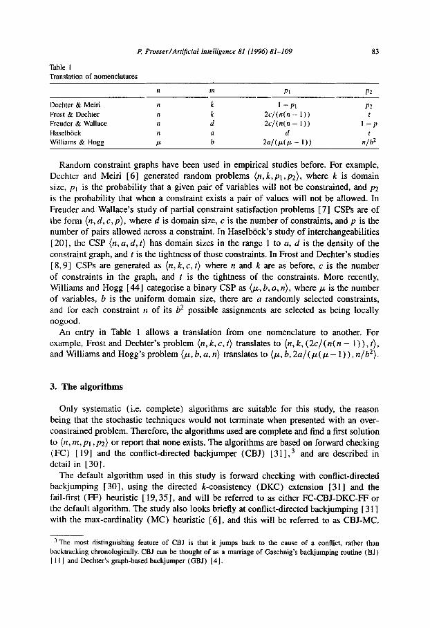
Table 1 Translation of nomenclatures

n m PI P2

Dechter & Meiri Frost & Dcchter Freuder & Wallace Haselbiick Williams & Hogg

1 -P1 2cl(n(n - 1)) Zc/(n(n - 1))

d

2alO-Q - 1))

P2 t

1-P t

n/b2

Random constraint graphs have been used in empirical studies before. For example, Dechter and Meiri [6] generated random problems (n, k,pt ,p*), where k is domain size, p1 is the probability that a given pair of variables will not be constrained, and p2 is the probability that when a constraint exists a pair of values will not be allowed. In Freuder and Wallace’s study of partial constraint satisfaction problems [7] CSPs are of the form (n, d, c, p), where d is domain size, c is the number of constraints, and p is the number of pairs allowed across a constraint. In Haselbock’s study of interchangeabilities [20], the CSP ( n, a, d, t) has domain sizes in the range 1 to a, d is the density of the constraint graph, and t is the tightness of those constraints. In Frost and Dechter’s studies [ 8,9] CSPs are generated as (n, k, c, t) where n and k are as before, c is the number of constraints in the graph, and t is the tightness of the constraints. More recently, Williams and Hogg [44] categorise a binary CSP as (p, b, a, n), where 1~ is the number of variables, b is the uniform domain size, there are a randomly selected constraints, and for each constraint n of its b2 possible assignments are selected as being locally nogood.

An entry in Table 1 allows a translation from one nomenclature to another. For example, Frost and Dechter’s problem (n, k, c, t) translates to (n, k, (2c/( n( n - 1) ) , t), and Williams and Hogg’s problem (,u, b, a, n) translates to (p, b, 2u/(,~( ,u- l)), n/b2).

3. The algorithms

Only systematic (i.e. complete) algorithms are suitable for this study, the reason being that the stochastic techniques would not terminate when presented with an over- constrained problem. Therefore, the algorithms used are complete and find a first solution to (n, m, PI , ~2) or report that none exists. The algorithms are based on forward checking (FC) [ 191 and the conflict-directed backjumper (CBJ) [ 311, 3 and are described in detail in [30].

The default algorithm used in this study is forward checking with conflict-directed backjumping [ 301, using the directed k-consistency (DKC) extension [ 311 and the fail-first (FF) heuristic [ 19,351, and will be referred to as either FC-CBJ-DKC-FP or the default algorithm. The study also looks briefly at conflict-directed backjumping [ 311 with the max-cardinality (MC) heuristic [6], and this will be referred to as CBJ-MC.

3 The most distinguishing feature of CBJ is that it jumps back to the cause of a conflict, rather than backtracking chronologically. CBJ can be thought of as a marriage of Gaschnig’s backjumping routine (BJ) I 1 I I and Dechter’s graph-based backjumper (GBJ) [4].

84 P Prosser/Art@cial Intelligence 81 (1996) 81-109

The selection of the default algorithm was based on previous computational experience [30-331.

The standard of comparison of constraint satisfaction algorithms has traditionally been the number of consistency checks performed, i.e. the number of times pairs of variable instantiations were tested for compatibility. The objective is then to reduce the number of consistency checks. Although it can be argued that this measure can be reduced by other means, such as constraint recording [9,10,16], this may lead to a trading of maintenance of that information against the cost of re-exploration. This has lead to an argument that run time should be taken as the standard of comparison [ 171. A previous study [ 301 showed that FC-CBJ performed less consistency checks and took less run time than other algorithms. The DKC extension and FF heuristic has lead to a further reduction in run time. Since the main thrust of this study is to examine problems, not algorithms, the fastest and most reliable algorithm was chosen, thus allowing the largest amount of experimentation possible.

The algorithms were initially encoded in Sun Common Lisp, SCLisp version 4.0, and run on SUN SPARCstation IPCs with 16MB of memory. In order to increase the rate that experiments could be performed the algorithms were later recoded in C [ 251. The Common Lisp implementation of the algorithms and problem generator are available electronically (see [ 341) .

4. The experiments

The first part of this study looks at what happens when we increase the tightness of constraints (pz), increase the density of the constraint graph (pt ), and change algorithms (from FC-CBJ-DKC-FF to CBJ-MC). The effect of the number of variables (n) and the domain size (m) is then investigated. The last subsection relates some of the computational experiences of the experiments.

4.1. Constraint tightness, graph density, and choice of algorithm

Problems were generated with 20 variables and a uniform domain size of 10. Col- lectively, these problems will be referred to by the tuple (20,lO). ‘Ihe density of the constraint graph, pt , was varied from 0.1 to 1 .O in steps of 0.1, and for each value of pr the constraint tightness p2 was varied from 0.01 to 0.99 in steps of 0.01.4 At each setting of (2O,lO,pt,p2) 100 problems were generated. The search algorithm was then applied to each problem. Numerous statistics were gathered, such as the search effort expended in terms of consistency checks, the number of backtracks, CPU time used, and whether the problem was soluble or insoluble. In total 99,000 (20,lO) problems were investigated.

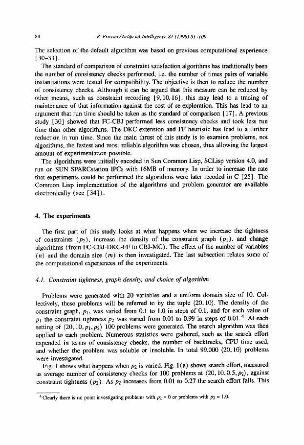
Fig. 1 shows what happens when pz is varied. Fig. 1 (a) shows search effort, measured as average number of consistency checks for 100 problems at (20,10,0.5,pz), against constraint tightness (~2). As p2 increases from 0.01 to 0.27 the search effort falls. This

4 Clearly there is no point investigating problems with p2 = 0 or problems with p2 = 1 .O.

P ProsserIArtijicial Intelligence 81 (I 996) 81-109 85

.5oocQ

45ooo

4oow

35000

3oooo

25000

20000

15000

10000

5000

n "0 0.1 0.2 0.3 0.4 0.5 0.6 0.7 0.8 0.9 1

P2

14OOOO -

120000 -

B looooo-

&ii 0 80000 -

60000 -

max - - mean ---

median ---- - st&” . . . . .

& -.-. _

0.2 0.25 0.3 0.35 0.4 0.45 0.5 0.55 0.6 0.65 0.7 P2

Fig. 1. Search effort against p2 for (20,10,0.5).

is due to the increasing effectiveness of domain filtering as pz increases. The onset of backtracking is at p2 M 0.25, and when p2 M 0.3 the search effort begins to increase rapidly, reaching a maximum at p2 x 0.38, and then falls away. 5 The vertical bar on the left-hand side is the largest value of p2 at which all problems were soluble (~2 = 0.35) and the right-hand vertical bar is the smallest value of p2 at which all problems were insoluble (~2 = 0.41). Therefore all problems to the left of the first vertical are soluble, and all problems to the right of the second vertical are insoluble. In the region between (i.e. 0.35 < pz < 0.41) there is a mixture of soluble and insoluble problems, and Smith has referred to this as the mushy region [ 37].6 It is in this region that the average search effort is maximal.

’ At p2 = 0.37, the average effort is 45,262 checks aad, at pz = 0.38, the average effort is 45,710 checks. ’ An analogy is drawn from the process of freezing, where an intermediate state is reached, neither liquid

nor solid.

86 P Prosser/Art$cial Intelligence 81 (1996) M-109

soluble problems - insoluble problems - - - _

mean .....-

0 0 5oooo lOOCOO 150000 2OcNm 25Oml

consistency checks

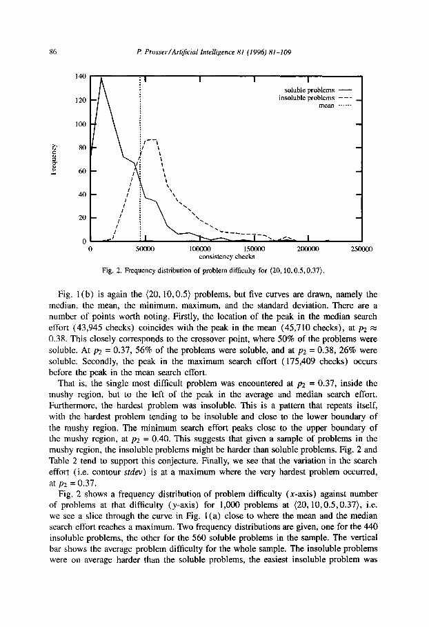
Fig. 2. Frequency distribution of problem difficulty for (20,10,0.5,0.37).

Fig. 1 (b) is again the (20,10,0.5) problems, but five curves are drawn, namely the

median, the mean, the minimum, maximum, and the standard deviation. There are a number of points worth noting. Firstly, the location of the peak in the median search

effort (43,945 checks) coincides with the peak in the mean (45,710 checks), at p2 M

0.38. This closely corresponds to the crossover point, where 50% of the problems were

soluble. At p2 = 0.37, 56% of the problems were soluble, and at p2 = 0.38, 26% were

soluble. Secondly, the peak in the maximum search effort (175,409 checks) occurs before the peak in the mean search effort.

That is, the single most difficult problem was encountered at p2 = 0.37, inside the mushy region, but to the left of the peak in the average and median search effort. Furthermore, the hardest problem was insoluble. This is a pattern that repeats itself,

with the hardest problem tending to be insoluble and close to the lower boundary of

the mushy region. The minimum search effort peaks close to the upper boundary of the mushy region, at p2 = 0.40. This suggests that given a sample of problems in the mushy region, the insoluble problems might be harder than soluble problems. Fig. 2 and Table 2 tend to support this conjecture. Finally, we see that the variation in the search

effort (i.e. contour S&V) is at a maximum where the very hardest problem occurred,

at p2 = 0.37. Fig. 2 shows a frequency distribution of problem difficulty (x-axis) against number

of problems at that difficulty (y-axis) for 1,000 problems at (20,10,0.5,0.37), i.e. we see a slice through the curve in Fig. 1 (a) close to where the mean and the median search effort reaches a maximum. Two frequency distributions are given, one for the 440 insoluble problems, the other for the 560 soluble problems in the sample. The vertical bar shows the average problem difficulty for the whole sample. The insoluble problems were on average harder than the soluble problems, the easiest insoluble problem was

P: Prosser/Artijicial Intelligence 81 (1996) 81-109 87

Table 2

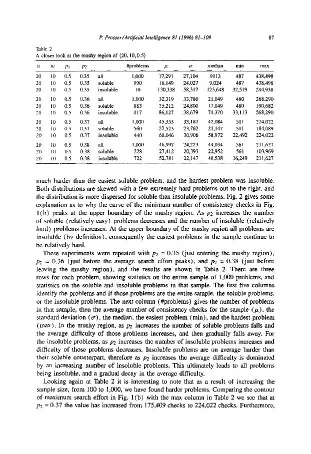
A closer look at the mushy region of (20,10,0.5)

,I m PI P2 #problems P u median min max

20 IO 0.5 0.35 all 1,000 17,291 27,104 9113 487 438,498

20 IO 0.5 0.35 soluble 990 16,149 24,027 9,024 487 438,498

20 IO 0.5 0.35 insoluble IO 130,338 58,317 123,648 32,519 244,938

20 10 0.5 0.36 all I.000 32,319 33,780 21,049 480 268,290

20 IO 0.5 0.36 soluble 883 25,212 24,800 17,049 480 190,682

20 10 0.5 0.36 insoluble I I7 86,127 38,679 74,370 33,l I3 268,290

20 IO 0.5 0.37 all 1,000 45,353 33,187 42,084 511 224,022

20 10 0.5 0.37 soluble 560 27,523 23,762 21,147 511 184,089

20 IO 0.5 0.37 insoluble 440 68,046 30,906 58,972 22,492 224,022

20 IO 0.5 0.38 all 1,000 46,997 24,223 44,034 561 211,627

20 IO 0.5 0.38 soluble 228 27,412 20,393 22,952 561 103,969

20 IO 0.5 0.38 insoluble 722 52.78 1 22,147 48,538 16,249 211,627

much harder than the easiest soluble problem, and the hardest problem was insoluble. Both distributions are skewed with a few extremely hard problems out to the right, and

the distribution is more dispersed for soluble than insoluble problems. Fig. 2 gives some

explanation as to why the curve of the minimum number of consistency checks in Fig.

1 (b) peaks at the upper boundary of the mushy region, As p2 increases the number of soluble (relatively easy) problems decreases and the number of insoluble (relatively hard) problems increases. At the upper boundary of the mushy region all problems are insoluble (by definition), consequently the easiest problems in the sample continue to

be relatively hard.

These experiments were repeated with p2 = 0.35 (just entering the mushy region), p2 = 0.36 (just before the average search effort peaks), and p2 = 0.38 (just before

leaving the mushy region), and the results are shown in Table 2. There are three rows for each problem, showing statistics on the entire sample of 1,000 problems, and statistics on the soluble and insoluble problems in that sample. The first five columns

identify the problems and if those problems are the entire sample, the soluble problems,

or the insoluble problems. The next column (#problems) gives the number of problems in that sample, then the average number of consistency checks for the sample (p), the standard deviation (a), the median, the easiest problem (min), and the hardest problem

(max). In the mushy region, as pz increases the number of soluble problems falls and

the average difficulty of those problems increases, and then gradually falls away. For the insoluble problems, as p2 increases the number of insoluble problems increases and

difficulty of those problems decreases. Insoluble problems are on average harder than their soluble counterpart, therefore as p2 increases the average difficulty is dominated by an increasing number of insoluble problems. This ultimately leads to all problems being insoluble, and a gradual decay in the average difficulty.

Looking again at Table 2 it is interesting to note that as a result of increasing the sample size, from 100 to 1,000, we have found harder problems. Comparing the contour of maximum search effort in Fig. l(b) with the max column in Table 2 we see that at p2 = 0.37 the value has increased from 175,409 checks to 224,022 checks. Furthermore,

88 P. Pro.~.~er/Art~cial Intelligence 81 (1996) 81-109

le+o5 L I I I I I I I I I J

fc-cbj-dkc-ff - ‘\

le+O6 r .’ ., cbj-mc - - - *

.I * \

10 I I I I I I I I I 0 0.1 0.2 0.3 0.4 0.5 0.6 0.7 0.8 0.9 1

P2

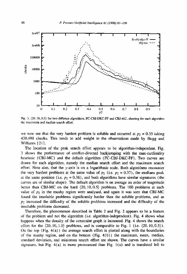
Fig. 3. (20,lO.O.S) for two different algorithms, FC-CBJ-DKC-FF and CBJ-MC, showing for each algorithm

the maximum and median search effort.

we now see that the very hardest problem is soluble and occurred at p2 = 0.35 taking 438,498 checks. This tends to add weight to the observations made by Hogg and Williams [ 211.

The location of the peak search effort appears to be algorithm-independent. Fig.

3 shows the performance of conflict-directed backjumping with the max-cardinality heuristic (CBJ-MC) and the default algorithm (FC-CBJ-DKC-FF). Two curves are

drawn for each algorithm, namely the median search effort and the maximum search effort. Note also, that the y-axis is on a logarithmic scale. Both algorithms encounter

the very hardest problems at the same value of p2 (i.e. p2 = 0.37), the medians peak at the same position (i.e. p2 = 0.38), and both algorithms have similar signatures (the

curves are of similar shape). The default algorithm is on average an order of magnitude

better than CBJ-MC on the hard (20,10,0.5) problems. The 100 problems at each value of p2 in the mushy region were analysed, and again it was seen that CBJ-MC found the insoluble problems significantly harder than the soluble problems, and as p2 increased the difficulty of the soluble problems increased and the difficulty of the

insoluble problems decreased. Therefore, the phenomenon described in Table 2 and Fig. 2 appears to be a feature

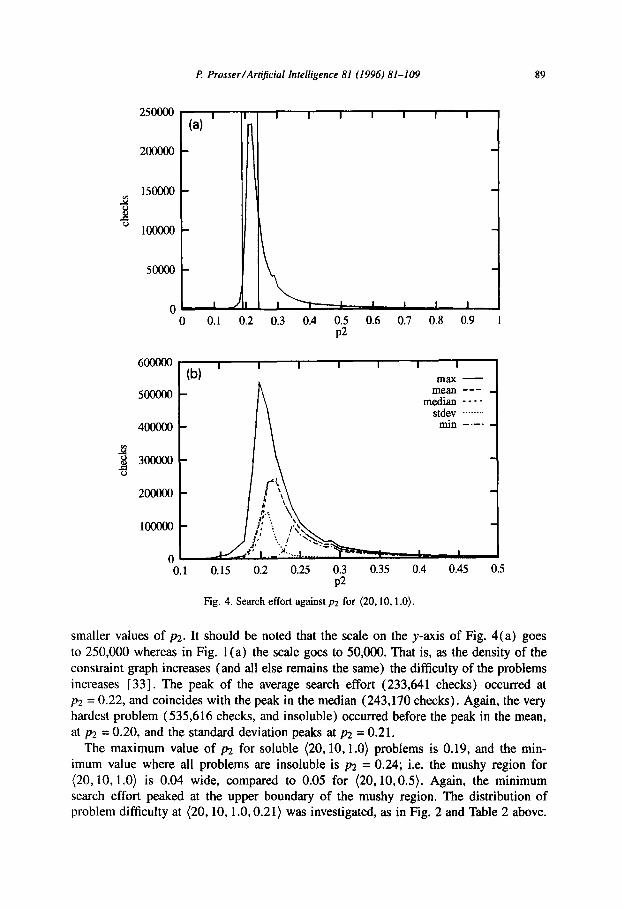
of the problem and not the algorithm (i.e. algorithm-independent). Fig. 4 shows what happens when the density of the constraint graph is increased. Fig. 4 shows the search effort for the (20,10,1.0) problems, and is comparable to Fig. 1 (i.e. (20,10,0.5)). On the top (Fig. 4(a)) the average search effort is plotted along with the boundaries of the mushy region, and on the bottom (Fig. 4(b)) the maximum, mean, median,

standard deviation, and minimum search effort are shown. The curves have a similar signature, but Fig. 4(a) is more pronounced than Fig. l(a) and is translated left to

P Prosser/Art@cial Intelligence 81 (1996) 81-109

250000

200000

150000 9

J.! ” 1OOOOo

5OcoO

0

GO0000

mo00

1OOOOO

n

0 0.1 0.2 0.3 0.4 0.5 0.6 0.7 0.8 0.9 1 P2

(b) I I I I I I I max -

mean --- - median ----

&jev . . . . . . . fin -.-. _

“0.1 0.15 0.2 0.25 0.3 0.35 0.4 0.45 0.5 P2

Fig. 4. Search effort against p2 for (20.10.1.0).

smaller values of p2. It should be noted that the scale on the y-axis of Fig. 4(a) goes to 250,000 whereas in Fig. 1 (a) the scale goes to 50,000. That is, as the density of the constraint graph increases (and all else remains the same) the difficulty of the problems increases [33]. The peak of the average search effort (233,641 checks) occurred at p2 = 0.22, and coincides with the peak in the median (243,170 checks). Again, the very hardest problem (535,616 checks, and insoluble) occurred before the peak in the mean, at p2 = 0.20, and the standard deviation peaks at p2 = 0.21.

The maximum value of pz for soluble (20,10,1.0) problems is 0.19, and the min- imum value where all problems are insoluble is p2 = 0.24; i.e. the mushy region for (20,10,1.0) is 0.04 wide, compared to 0.05 for (20,10,0.5). Again, the minimum search effort peaked at the upper boundary of the mushy region. The distribution of problem difficulty at (20,10,1 .O, 0.21) was investigated, as in Fig. 2 and Table 2 above.

90

le+O6

P. Prosser/Artij?cial Intelligence 81 (1996) 81-109

<20.10,0.1>

100 0 0.1 0.2 0.3 0.4 0.5 0.6 0.7 0.8 0.9 1

le+O6

IooooO

10000

<20.10,0.2>

(b) ' 1 I I I I I I I

1

loo0

100 0 0.1 0.2 0.3 0.4 0.5 0.6 0.7 0.8 0.9 1

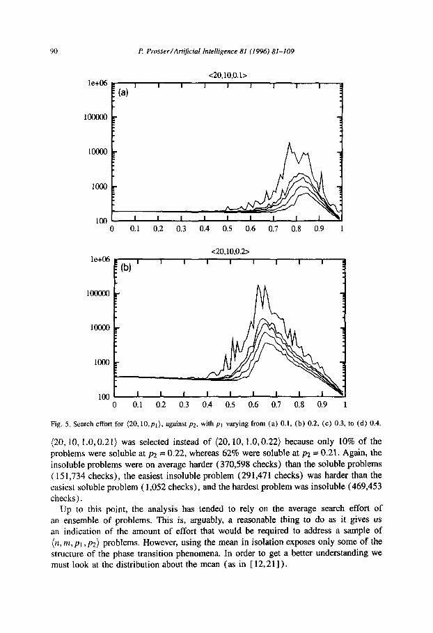
Fig. 5. Search effort for (2O,lO,pt), against ~2, with p1 varying from (a) 0.1, (b) 0.2, (c) 0.3, to (d) 0.4.

(20,10,1.0,0.21) was selected instead of (20,10,1.0,0.22) because only 10% of the problems were soluble at p2 = 0.22, whereas 62% were soluble at p2 = 0.21. Again, the insoluble problems were on average harder (370,598 checks) than the soluble problems ( 15 1,734 checks), the easiest insoluble problem (291,47 1 checks) was harder than the easiest soluble problem ( 1,052 checks), and the hardest problem was insoluble (469,453 checks).

Up to this point, the analysis has tended to rely on the average search effort of an ensemble of problems. This is, arguably, a reasonable thing to do as it gives us an indication of the amount of effort that would be required to address a sample of (n, m, pi, ~2) problems. However, using the mean in isolation exposes only some of the structure of the phase transition phenomena. In order to get a better understanding we must look at the distribution about the mean (as in [ 12,211).

R Prosser/Artifcial Intelligence 81 (1996) 81-109 91

le+O6 <20,10,0.3>

1000

100 0 0.1 0.2 0.3 0.4 0.5 0.6 0.7 0.8 0.9 1

<20,10,0.4> le+O6

IO0000

loo0

100 0 0.1 0.2 0.3 0.4 0.5 0.6 0.7 0.8 0.9 1

Cd) Fig. 5 -continued.

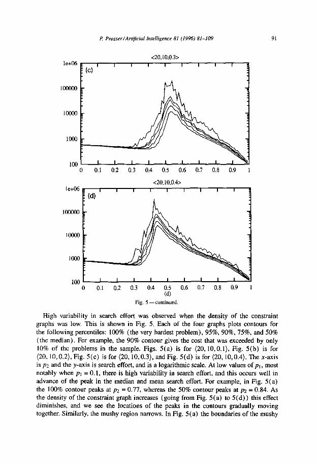
High variability in search effort was observed when the density of the constraint graphs was low. This is shown in Fig. 5. Each of the four graphs plots contours for the following percentiles: 100% (the very hardest problem), 95%, 90%, 75%, and 50% (the median). For example, the 90% contour gives the cost that was exceeded by only 10% of the problems in the sample. Figs. 5(a) is for (20,lO.O. 1). Fig. 5(b) is for (20,10,0.2), Fig. 5(c) is for (20,10,0.3), and Fig. 5(d) is for (20,10,0.4). The x-axis is p2 and the y-axis is search effort, and is a logarithmic scale. At low values of pr , most notably when pi = 0.1, there is high variability in search effort, and this occurs well in advance of the peak in the median and mean search effort. For example, in Fig. 5(a) the 100% contour peaks at p2 = 0.77, whereas the 50% contour peaks at p2 = 0.84. As the density of the constraint graph increases (going from Fig. 5 (a) to 5 (d) ) this effect diminishes, and we see the locations of the peaks in the contours gradually moving together. Similarly, the mushy region narrows. In Fig. 5(a) the boundaries of the mushy

92 P Prosser/Art@cial Intelligence 81 (1996) 81-109

checks

(4

xO000 -

1.50000 -

100000 -

50000 -

0

(b)

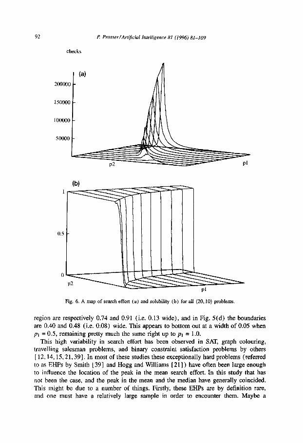
-7 Fig. 6. A map of search effort (a) and solubility (b) for ail (20.10) problems.

region are respectively 0.74 and 0.91 (i.e. 0.13 wide), and in Fig. 5 (d) the boundaries are 0.40 and 0.48 (i.e. 0.08) wide. This appears to bottom out at a width of 0.05 when pi = 0.5, remaining pretty much the same right up to pt = 1.0.

This high variability in search effort has been observed in SAT, graph colouring, travelling salesman problems, and binary constraint satisfaction problems by others [ 12,14,15,21,39]. In most of these studies these exceptionally hard problems (referred to as EHPs by Smith [ 391 and Hogg and Williams [ 211) have often been large enough to influence the location of the peak in the mean search effort. In this study that has not been the case, and the peak in the mean and the median have generally coincided. This might be due to a number of things. Firstly, these EHPs are by definition rare, and one must have a relatively large sample in order to encounter them. Maybe a

R Prosser/Art$cial Intelligence 81 (1996) 81-109 93

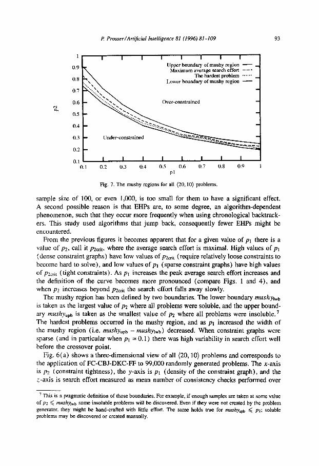
1 I I I I I I I I Upper boundary of mushy region - _

Maximum average search effort --- The hardest problem ..__._ _

Lower boundary of mushy region -

Over-constrained

0.3 -

0.2 -

Under-constrained

0.1 I I I I I I I I

0.1 0.2 0.3 0.4 0.5 0.6 0.7 0.8 0.9 1 Pl

Fig. 7. The mushy regions for all (20.10) problems.

sample size of 100, or even 1,000, is too small for them to have a significant effect. A second possible reason is that EHPs are, to some degree, an algorithm-dependent phenomenon, such that they occur more frequently when using chronological backtrack- ers. This study used algorithms that jump back, consequently fewer EHPs might be encountered.

From the previous figures it becomes apparent that for a given value of pt there is a value of ~2, call it pzc,+r, where the average search effort is maximal. High values of pt (dense constraint graphs) have low values of pzctit (require reIatively loose constraints to become hard to solve), and low values of pt (sparse constraint graphs) have high values of p2crit (tight constraints). As pr increases the peak average search effort increases and the definition of the curve becomes more pronounced (compare Figs. 1 and 4), and when p2 increases beyond pzc,.k the search effort falls away slowly.

The mushy region has been defined by two boundaries. The lower boundary mushylwb is taken as the largest value of p2 where all problems were soluble, and the upper bound- ary mUShy@, is taken as the smallest value of pz where all problems were insoluble.7 The hardest problems occurred in the mushy region, and as pi increased the width of the mushy region (i.e. mushyupb - mushylwb) decreased. When constraint graphs were sparse (and in particular when p1 = 0.1) there was high variability in search effort well before the crossover point.

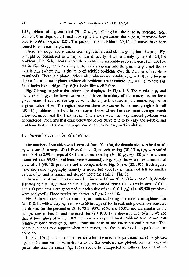
Fig. 6(a) shows a three-dimensional view of all (20,lO) problems and corresponds to the application of FC-CBJ-DKC-FF to 99,000 randomly generated problems. The x-axis

is p2 (constraint tightness), the y-axis is PI (density of the constraint graph), and the z-axis is search effort measured as mean number of consistency checks performed over

’ This is a pragmatic definition of those boundaries. For example, if enough samples are taken at some value of p2 < mushytwt, some insoluble problems will be discovered. Even if they were not created by the problem generator, they might be hand-crafted with little effort. The same holds true for rnu~hy,~t, < ~2; soluble problems may be discovered or created manually.

94 P Prosser/Art@ial Intelligence 81 (1996) 81-109

100 problems at a given point (20,10, PI, ~2). Going into the page p1 increases from 0.1 to 1.0 in steps of 0.1, and moving left to right across the page p2 increases from 0.01 to 0.99 in steps of 0.01. The peaks of the individual (2O,lO,pl) curves have been joined to enhance the picture.

There is a ridge, and it tracks from right to left and climbs going into the page. Fig. 6 might be considered as a map of the difficulty of all randomly generated (20,lO) problems. Fig. 6(b) shows where the soluble and insoluble problems exist for (20,lO). As in Fig. 6(a), the x-axis is ~2, the y-axis (going into the page) is ~1, and the Z- axis is psOl (where psOl is the ratio of soluble problems over the number of problems examined). There is a plateau where all problems are soluble ( psOl = 1 .O), and then an abrupt fall to a lower plateau where all problems are insoluble (p,,l = 0.0). Where Fig. 6(a) looks like a ridge, Fig. 6(b) looks like a cliff face.

Fig. 7 brings together the information displayed in Figs. l-6. The x-axis is PI and the y-axis is ~2. The lower curve is the lower boundary of the mushy region for a given value of ~1, and the top curve is the upper boundary of the mushy region for a given value of pl. The region between these two curves is the mushy region for all (20, 10) problems, the bold broken curve shows where the maximum average search effort occurred, and the faint broken line shows were the very hardest problem was encountered. Problems that exist below the lower curve tend to be easy and soluble, and problems that exist above the upper curve tend to be easy and insoluble.

4.2. Increasing the number of variables

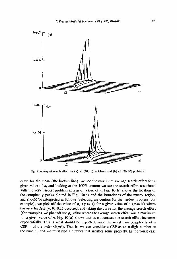
The number of variables was increased from 20 to 30, the domain size was held at 10, pl was varied in steps of 0.1 from 0.1 to 1.0, at each setting (30,10, ~1) p2 was varied from 0.01 to 0.99 in steps of 0.01, and at each setting (3O,lO,pl ,p2) 100 problems were examined (i.e. 99,000 problems were examined). Fig. 8 (a) shows a three-dimensional view of all (30,lO) problems and is comparable to Fig. 6 (i.e. (20,lO)). Both figures have the same topography, namely a ridge, but (30,lO) is translated left to smaller values of p2 and is higher and steeper (note the scale in Fig. 8).

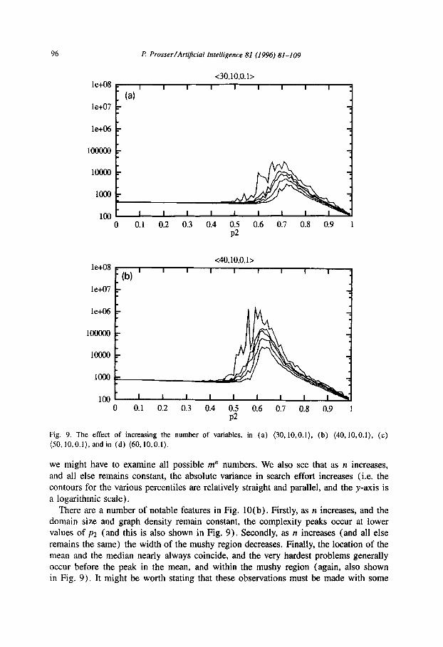
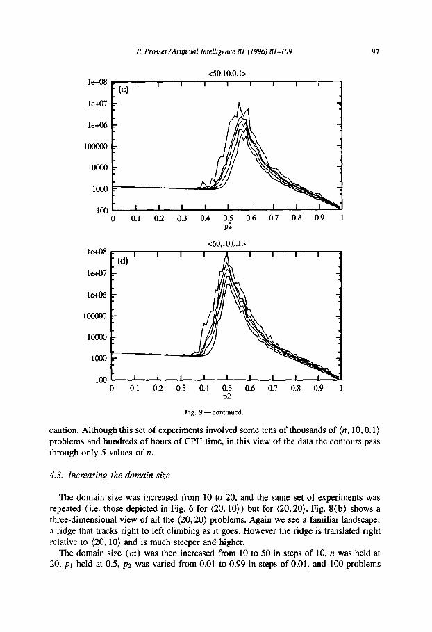
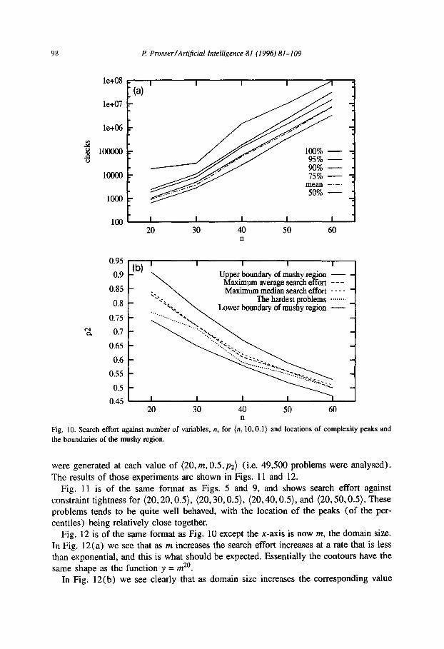
The number of variables (n) was then increased from 20 to 60 in steps of 10, domain size was held at 10, pi was held at 0.1, p2 was varied from 0.01 to 0.99 in steps of 0.01, and 100 problems were generated at each value of (n, 10,O. l,pz) (i.e. 49,500 problems were analysed). These results are shown in Figs. 9 and 10.

Fig. 9 shows search effort (on a logarithmic scale) against constraint tightness for (n, 10,O. l), with n varying from 30 to 60 in steps of 10. In each sub-picture five contours are drawn, for the percentiles 50%, 75%, 90%, 95%, and lOO%, and are similar to the sub-pictures in Fig. 5 (and the graph for (20,10,0.1) is shown in Fig. 5(a)). We see that at low values of n the 100% contour is noisy, and hard problems tend to occur at relatively low values of ~2, away from the peak of the lower percentile curves. This behaviour tends to disappear when n increases, and the locations of the peaks tend to coincide.

In Fig. 10(a) the maximum search effort (y-axis, a logarithmic scale) is plotted against the number of variables (x-axis). Six contours are plotted, for the range of percentiles and the mean. Fig. 10(a) should be interpreted as follows. Looking at the

i? Prosser/Art$cial Intelligence 81 (1996) 81-109 95

le+07

5e+O6

le+07

5e+O6

0

(b)

P2

Fig. 8. A map of search effort for (a) all (30.10) problems, and (b) all (20.20) problems.

curve for the mean (the broken line), we see the maximum average search effort for a

given value of n, and looking at the 100% contour we see the search effort associated with the very hardest problem at a given value of n. Fig. 10(b) shows the location of

the complexity peaks plotted in Fig. 10(a) and the boundaries of the mushy region, and should be interpreted as follows. Selecting the contour for the hardest problem (for example), we pick off the value of p2 (y-axis) for a given value of IZ (x-axis) where the very hardest (n, 10,O.l) occurred, and taking the curve for the average search effort (for example) we pick off the pz value where the average search effort was a maximum

for a given value of n. Fig. 10(a) shows that as n increases the search effort increases exponentially. This is what should be expected, since the worst case complexity of a CSP is of the order O(m”). That is, we can consider a CSP as an n-digit number to the base m, and we must find a number that satisfies some property. In the worst case

96

le+08

le+O7

le+O6

le+08

le+O7

le+O6

1OOOMJ

loo00

I? Prosser/Artifcial Intelligence 81 (1996) M-109

<30,10,0.1>

0 0.1 0.2 0.3 0.4 0.5 0.6 0.7 0.8 0.9 1 P2

<40,10,0.1> \ : (b) ’

I I I 1 I I I I d

1oixl

100 0 0.1 0.2 0.3 0.4 0.5 0.6 0.7 0.8 0.9 1

P2

Fig. 9. The effect of increasing the number of variables, in (a) (30,10,0.1), (b) (40,10,0.1), (c) (SO,lO,O.l),andin (d) (60,lO.O.l).

we might have to examine all possible m” numbers. We also see that as n increases, and all else remains constant, the absolute variance in search effort increases (i.e. the

contours for the various percentiles are relatively straight and parallel, and the y-axis is a logarithmic scale).

There are a number of notable features in Fig. IO(b). Firstly, as n increases, and the domain size and graph density remain constant, the complexity peaks occur at lower values of p2 (and this is also shown in Fig. 9). Secondly, as n increases (and all else

remains the same) the width of the mushy region decreases. Finally, the location of the mean and the median nearly always coincide, and the very hardest problems generally occur before the peak in the mean, and within the mushy region (again, also shown in Fig. 9). It might be worth stating that these observations must be made with some

P Prosser/Artifcial Intelligence 81 (1996) U-109 97

le+O8

le+O7

le+O6

1OOOOO

10000

1000

100

le+O8

le+O7

le+O6

1OOOOO

10000

1000

100

0 0.1 0.2 0.3 0.4 0.5 0.6 0.7 0.8 0.9 1 P2

<60,10.0.1>

0 0.1 0.2 0.3 0.4 0.5 0.6 0.7 0.8 0.9 1 P2

Fig. 9 -continued.

caution. Although this set of experiments involved some tens of thousands of (n, 10,O. 1) problems and hundreds of hours of CPU time, in this view of the data the contours pass through only 5 values of II.

4.3. tncreasing the domain size

The domain size was increased from 10 to 20, and the same set of experiments was repeated (i.e. those depicted in Fig. 6 for (20,lO)) but for (20,20). Fig. 8(b) shows a three-dimensional view of all the (20,20) problems. Again we see a familiar landscape; a ridge that tracks right to left climbing as it goes. However the ridge is translated right relative to (20, IO) and is much steeper and higher.

The domain size (m) was then increased from 10 to 50 in steps of 10, n was held at 20, pt held at 0.5, p2 was varied from 0.01 to 0.99 in steps of 0.01, and 100 problems

P. Pmsser/Artifcial Intelligence 81 (1996) M-109

le+08

le+O7

le+M

lcrOOO0

1OOOO

1OUO

100 t I I I I I 1 20 30 40 50 60

n

0.95

0.9 Jb'

I I I I I

0.85 -

0.8 -

0.75 - N a 0.7 -

0.65 -

0.6 -

0.55 -

0.5 -

0.45 20 30 40 50 60

n

Fig, 10. Search effort against number of variables, n, for (n, 10.0.1) and locations of complexity peaks and the boundaries of the mushy region.

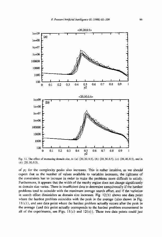
were generated at each value of (20, m, 0.5,~~) (i.e. 49,500 problems were analysed).

The results of those experiments are shown in Figs. 11 and 12. Fig. I1 is of the same format as Figs. 5 and 9, and shows search effort against

constraint tightness for (20,20, OS), (20,30,0.5), (20,40,0.5), and (20,50,0.5). These problems tends to be quite well behaved, with the location of the peaks (of the per- centiles) being relatively close together.

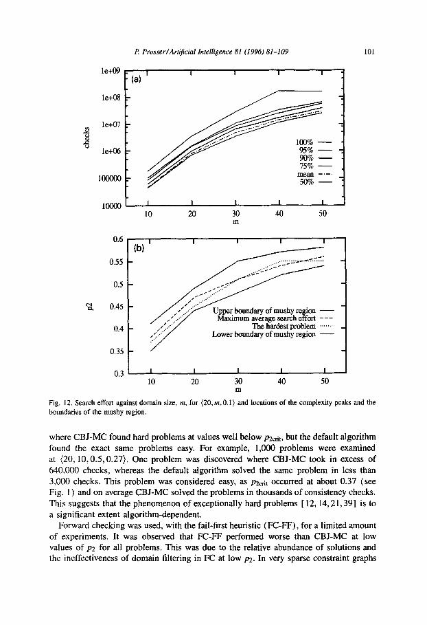
Fig. 12 is of the same format as Fig. 10 except the x-axis is now m, the domain size. In Fig. 12(a) we see that as m increases the search effort increases at a rate that is less than exponential, and this is what should be expected. Essentially the contours have the same shape as the function y = m*'.

In Fig. 12(b) we see clearly that as domain size increases the corresponding value

P: Presser/Artificial Intelligence 81 (1996) 81-109 99

le+O9

le+08

le+07

le+O6

1000

100 0 0.1 0.2 0.3 0.4 0.5 0.6 0.7 0.8 0.9 1

P2

le+O9 <20,30,0.5>

le+08

le+07

le+O6

1000

100 0 0.1 0.2 0.3 0.4 0.5 0.6 0.7 0.8 0.9 1

P2

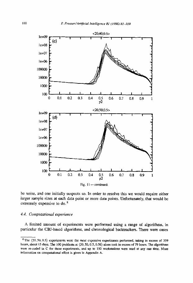
Fig. I 1. The effect of increasing domain size, in (a) (20,20,0.5), (b) (20,30, OS), (c) (20,40, OS), and in (d) (20,5O,O.S).

of p2 for the complexity peaks also increases. This is rather intuitive, as we should expect that as the number of values available to variables increases, the tightness of

the constraints has to increase in order to make the problems more difficult to satisfy. Furthermore, it appears that the width of the mushy region does not change significantly as domain size varies. There is insufficient data to determine unequivocally if the hardest problems tend to coincide with the maximum average search effort, and if the variation in search effort diminishes as domain size increases. Fig. 12(b) shows one data point where the hardest problem coincides with the peak in the average (also shown in Fig. 11 (c) > , and one data point where the hardest problem actually occurs after the peak in the average (and this point actually corresponds to the hardest problem encountered in all of the experiments, see Figs. 11 (c) and 12(a)). These two data points could just

100 P Prosser/Artijicial Intelligence 81 (1996) 81409

le+O9

le+O8

le+07

le+O6

1OOOOO

10000

1000

100

<20,40,0.5>

0 0.1 0.2 0.3 0.4 0.5 0.6 0.7 0.8 0.9 1 P2

le+O9

le+O8

le+07

le+O6

1OOOOO

10000

1000

100 0 0.1 0.2 0.3 0.4 0.5 0.6 0.7 0.8 0.9 1

P2

Fig. 1 I - continued.

be noise, and one initially suspects so. In order to resolve this we would require either larger sample sizes at each data point or more data points. Unfortunately, that would be extremely expensive to do. 8

4.4. Computational experience

A limited amount of experiments were performed using a range of algorithms, in particular the CBJ-based algorithms, and chronological backtrackers. There were cases

s The (20,50,0.5) experiments were the most expensive experiments performed, taking in excess of 359 hours, about 15 days. The 100 problems at (20,50,0.5,0.56) alone took in excess of 79 hours. The algorithms were re-coded in C for these experiments, and up to 150 workstations were used at any one time. Mom information on computational effort is given in Appendix A.

P: Prosser/ArtijScial Intelligence 81 (1996) N-109 101

le+O9 L

- (a) ’

le+07 :

10000 I I I I I

10 20 30 40 50 m

0.6 I I I I I (b)

0.55 -

0.5 -

cu a 0.45 -

0.4 - Lower boundary of mushy region -

0.35 -

0.3 I I I I I

10 20 30 40 50 m

Fig. 12. Search effort against domain size, tn. for (20, m, 0.1) and locations of the complexity peaks and the boundaries of the mushy region.

where CBJ-MC found hard problems at values well below Pzc,.tt, but the default algorithm found the exact same problems easy. For example, 1,000 problems were examined at (20,10,0..5,0.27). One problem was discovered where CBJ-MC took in excess of 640,000 checks, whereas the default algorithm solved the same problem in less than 3,000 checks. This problem was considered easy, as Bcrit occurred at about 0.37 (see Fig. 1) and on average CBJ-MC solved the problems in thousands of consistency checks. This suggests that the phenomenon of exceptionally hard problems [ 12,14,21,39] is to a significant extent algorithm-dependent.

Forward checking was used, with the fail-first heuristic (FC-IF), for a limited amount of experiments. It was observed that FC-FF performed worse than CBJ-MC at low values of p2 for all problems. This was due to the relative abundance of solutions and the ineffectiveness of domain filtering in FC at low ~2. In very sparse constraint graphs

102 P Prosser/Artijicial Intelligence 81 (1996) 81-109

(pt = 0.1) CBJ-MC was much better than FC-FF, and this was due to the difference between backjumping and chronological backtracking. It is a conjecture, that in order for an algorithm to perform well in sparse constraint graphs, it must be able to jump about the search space freely. When pt increased (beyond pt = 0.3) the difference in performance between FC-FF and the default algorithm became insignificant. It is a conjecture that this is due to the fail-first heuristic exposing dependencies; i.e. given a uniform domain size, when choosing the current variable fail-first will select a variable that has been filtered by some past variable, consequently when backtracking on failure the algorithm tends to fall back on a dependent variable.

Forward checking without the fail-first heuristic was almost always hopelessly ineffi- cient. For example, the (20,10,0.1) experiments were re-run with 50 problems at each point (i.e. 4,950 problems), using the algorithms fc, FC-FF, FC-CBJ, and FC-CBJ-FF. Without the FF heuristic FC took 574 hours and FC-CBJ took 14 minutes. With the FF heuristic FC-FF took 6 minutes and FC-CBJ-FF took 2 minutes. The algorithms were encoded in C for these experiments [ 251. However, there were particular cases where using the fail-first heuristic degraded performance. When constraints are loose (low values of ~2) it is in fact beneficial to choose as the current variable the one with most values remaining in its domain. Consequently when instantiating the current variable there are fewer variable/value pairs to check against in the future. Admittedly this may sound a bit artificial, but it suggests that when a problem is loosely constrained, constraint propagation may be wasteful (just check backwards), but if propagation is used then propagate from variables with large domains to variables with small domains. More information on the run time of the experiments is given in Appendix A.

5. Comparison with the theory

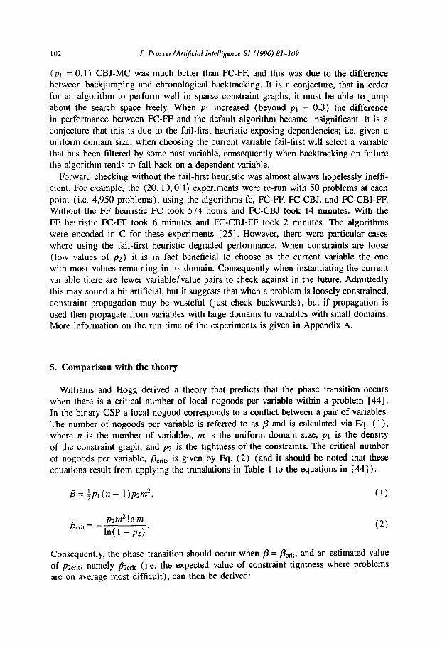
Williams and Hogg derived a theory that predicts that the phase transition occurs when there is a critical number of local nogoods per variable within a problem [44]. In the binary CSP a local nogood corresponds to a conflict between a pair of variables. The number of nogoods per variable is referred to as p and is calculated via Eq. ( 1 ), where n is the number of variables, m is the uniform domain size, pt is the density of the constraint graph, and p2 is the tightness of the constraints. The critical number of nogoods per variable, flcrtr, is given by Eq. (2) (and it should be noted that these equations result from applying the translations in Table 1 to the equations in [ 441).

P= $pl(n- l)p2m2, (1)

pcrit = _ mm2 In m Ml -p2)’

(2)

Consequently, the phase transition should occur when p = Pcrtr, and an estimated value of /V_crit, namely @?crtt (i.e. the expected value of constraint tightness where problems are on average most difficult), can then be derived:

R Prosser/Art#cial Intelligence 81 (1996) 81-109 103

0.8

0.7

0.6 Pi c

0.5

0.4

0.3

0.2

0.1

<20,20> Expected + - Empirical i--

<20,10> Expected a- Empirical s - -

<30,10> Expected -AS.- Empirical SC-’ _

I I I I

0.2 0.4 0.6 0.8 1 Pl

Fig. 13. Expected and empirical results.

P = &it,

1 ZPl (n - 1 )&itm2 = -

.&ritm* In 112

ln( 1 - B~~ri0 ’ P^2crit = 1 _ m-*/Pl(n-l) (3)

It should be noted that &it has been derived by different means. Smith [37,38] conjectures that the phase transition occurs when problems have, on average, just one solution. Given a binary CSP (n, m, ~1, ~2) an arbitrary instantiation of the variables will be a solution if all $ptn(n - 1) constraints are satisfied. There are m” possi- ble instantiations of the variable. Therefore, the expected number of solutions, E(N), is:

E(N) = m”( ] _ p2)Pln(n-1)/2 (4)

and the most difficult problems might occur when E(N) = 1, such that there is a mixture of insoluble problems and problems which have very few solutions, there- fore

1 = m”( 1 - fi2crit)Pln(n-1)/2, (5)

and this reduces to Eq. (3) above.

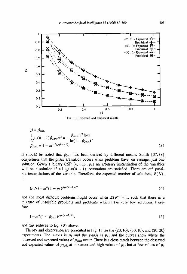
Theory and observation are presented in Fig. 13 for the (20, lo), (30, lo), and (20,20) experiments. The x-axis is pi and the y-axis is p2, and the curves show where the observed and expected values of pzctit occur. There is a close match between the observed and expected values of pzcet at moderate and high values of pr, but at low values of p1

104

Table 3

I? Prosser/Ar@cial Intelligence 81 (1996) 81-109

The effect of being connected

Problem PZcrit hit hnnected

(20,10,0.2) 0.66 0.70 0.74 0.67 1.00

(20, IO, 0.3) 0.54 0.55 0.97 0.52 1 .oo

(30,10,0.1) 0.72 0.80 0.25 0.72 1.00

(30, 10,0.2) 0.51 0.55 0.95 0.52 1 .oo

(40, 10,O.l) 0.63 0.69 0.49 0.63 1.00

(50,10,0.1) 0.56 0.61 0.75 (60,10,0.1) 0.50 0.54 0.87

there is a significant difference. 9 At low values of pt the hard problems occur earlier than expected. Experiments were performed to determine if this discrepancy might be due to the constraint graphs being disconnected. That is, if the graphs were disconnected they might appear to be made up of a smaller number of variables, and the actual density of the largest component may be greater than pt. This would then require a smaller value of p2 to become hard. The (20,10,0.2), (20,10,0.3), (30, lO,O.l), (30,10,0.2), and (40,10,0.1) experiments were then repeated but any disconnected constraint graphs were discarded. lo The results of those experiments are summarised in Table 3.

The column &onnecte,j is the ratio of connected constraint graphs over the number of constraint graphs examined. Where there are two row entries for a problem (n, m,pl), the first row corresponds to the experiments where constraint graphs were allowed to be disconnected, and the second row corresponds to experiments where discon- nected graphs were discarded (consequently p connected will be 1.0). As II increases (and as pl increases) the probability that the constraint graph is connected increases, and this is expected [ 1,291. Being connected does not appear to influence the outcome of the experiments; pzcrit and the location of the mushy region is generally unaf- fected. Although not shown, it did not significantly affect the average search effort either.

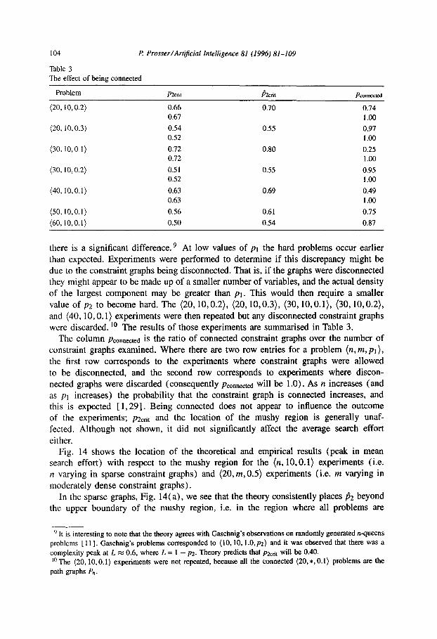
Fig. 14 shows the location of the theoretical and empirical results (peak in mean search effort) with respect to the mushy region for the (n, 10,O.l) experiments (i.e. n varying in sparse constraint graphs) and (20, m, 0.5) experiments (i.e. m varying in moderately dense constraint graphs).

In the sparse graphs, Fig. 14(a), we see that the theory consistently places $2 beyond the upper boundary of the mushy region, i.e. in the region where all problems are

‘) It is interesting to note that the theory agrees with Gaschnig’s observations on randomly generated n-queens problems [ 1 I]. Gaschnig’s problems corresponded to (10, 10, 1.0,~~) and it was observed that there was a complexity peak at L x 0.6, where L = 1 - pa. Theory predicts that p&d, will be 0.40. ‘” The (20.10.0.1) experiments were not repeated, because all the connected (20, *,O.l) problems are the path graphs Pn.

l? Prosser/Ar@cial Intelligence 81 (1996) M-109 105

0.8

Pi a 0.1

0.6

0.6

0.55

0.5

CI a 0.45

0.4

0.35

0.3

a) I I I I I

mushy upper boundary - . theory -o-- mean -t-

mushy lower boundary - .

20 30 40 50 60 tl

mushy upper boundary - theory +., mean -t-

mushy lower boundary -

I I I I I

10 20 30 40 50 m

Fig. 14. Comparison of empirical and theoretical results, for (a) (n, 10,O.l) and (b) (20,m,0.5).

insoluble. Conversely, in Fig. 14(b), theory matches the empirical results remarkably well; in fact, they are indistinguishable. One possible explanation for the discrepancy in Fig. 14(a) and the accuracy in Fig. 14(b) is as follows. The theory is based on the conjecture that on average the hardest problems will occur when on average there is a single solution. It may be the case that in sparse constraint graphs, at the crossover point problems either have very many solutions or none at all. Consequently, the average number of solutions is large at crossover, and it is only when constraints are tighter that problems have on average a single (or very few) solutions, and this will occur at the upper boundary of the mushy region. Conversely, in relatively dense constraint graphs, at the crossover point problems have either no solution or very few solutions. Consequently, theory becomes more accurate as density increases, and this agrees with Smith’s observations on the variance in the number of solutions [ 381.

106 P. Prosser/Art@cial Inielligence 81 (1996) 81-109

6. Conclusion

The study shows that for binary CSPs with n variables, uniform domain size m, and graph density pt , there is a critical value of constraint tightness ~2, namely pxcrtt, where

the average search effort is maximal, and this correspond closely to the crossover point

where 50% of the problems are soluble. The region where the phase transition takes place has been referred to as the mushy region, i.e. the region where problems change from being soluble to insoluble. As the density of the constraint graph increases the

width of the mushy region decreases and the maximal average search effort increases.

The hardest problem was generally encountered on first entering the mushy region, and that problem was generally insoluble. Within the mushy region the insoluble problems

were on average harder than the soluble problem. As p2 increased the soluble problems became scarce and more difficult, and insoluble problems became plentiful and less difficult. These phenomena appear to be characteristics of the problem i.e. they are

algorithm-independent. The landscape of the difficulty of some (n,m) problems have been mapped out and the topography is a ridge that curves from right to left, climbing

as it goes. It has been observed that in sparse constraint graphs (low values of PI) there is great

variability in search effort well before the phase transition. However, this variability was

not enough to inlluence the location of the peak in the mean search effort, the mean

occurring close to the peak in the median search effort. However, this might not be the

case if larger samples of problems were examined, or less informed algorithms were used. As the density of the constraint graph increases this variability diminishes.

The location of the greatest average difficulty, pzc,3, was predicted to occur when an ensemble of problems have on average one solution. The theory was accurate for

moderate to high values of pi, but in sparse graphs theory predicted that pzcrit would occur beyond the upper boundary of the mushy region, where all problems are insoluble.

One possible explanation for this is that in the mushy region sparse problems have either no solution or very many solutions. Consequently, in sparse graphs at the crossover point

the average number of solutions could be large, and it is only when nearly all problems

are insoluble that the average number of solutions is low. Conversely, in moderate to high densities it appears that at the crossover point problems either have no solutions or

very few solutions, and the theory is accurate. The theory may be used in a number of ways. The most obvious role is within an

empirical science of algorithms [ 221. As a starting point, p2crit may be considered as

a point of reference on the landscape, and algorithms may be positioned with respect to this. This might lead us to making informed choices as to what algorithm and heuristic to use for a given instance of a problem. Work in this area has already started [ 4 1 ] . Furthermore, by discovering under what circumstances one algorithm outperforms another we might gain a better understanding of the behaviour of algorithms, and this in turn should lead us to designs for even better algorithms and heuristics. Finally, this

might lead us to a better understanding of the structure of hard problems. Looking further ahead, if it is discovered that real world problems behave in a manner

predicted by the theory then it might allow us to move intelligent decision making into the realms of real time. For example, if we have a resource allocation problem

F! Prosser/Artijiciul Intelligence 81 (1996) 81-109 107

Table A.1

Computational cost of the experiments

Experiment

(20,lO)

(20, 10.0.5)

(20, 10.0.5)

(20, 10,0.5,0.35)

(20, 10,0.5,0.36)

(20, 10,0.5,0.37)

(20, 10,0.5,0.38)

(20, IO, 1 .O) (20,10,1.0,0.21)

(30, IO)

(30,10,0.1)

(40,10,0.1)

(50,10,0.1)

(60, 10,O.l)

(20,20)

(20.20,0.5)

(20,20,0.5)

(20,30,0.5)

(20.40.0.5)

(20,50,0.5)

#problems Implementation CPU time (hours)

99,000 SCLisp 4.0 38

9,900 SCLisp 4.0 1.4

9,900 SCLisp 4.0 CBJ-MC 18

1,000 SCLisp 4.0 1.2 1,000 SCLisp 4.0 2.4

1,000 SCLisp 4.0 3.5

1,000 SCLisp 4.0 3.4

9,900 SCLisp 4.0 8

1,000 SCLisp 4.0 13

99,000 ANSI C 115

9,900 ANSI C 0.6

9,900 ANSI C 2

9,900 ANSI C 13

9,900 ANSI C 86

99,000 ANSI C 188

9,900 SCLisp 4.0 90

9,900 ANSI C II

9,900 ANSI C 55

9,900 ANSI C 135

9,900 ANSI C 359

characterised as (n, m, pt , pz), in the event that p2 > &.tt we might know (with some confidence) that the problem is over-constrained. What is more relevant is that we might know how far the problem should be relaxed such that it becomes soluble, and possibly easy.

Appendix A. Computational effort

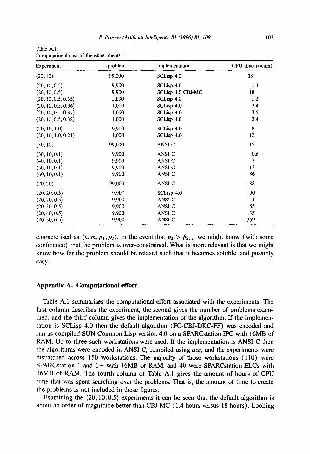
Table A.1 summarises the computational effort associated with the experiments. The first column describes the experiment, the second gives the number of problems exam- ined, and the third column gives the implementation of the algorithm. If the implemen- tation is SCLisp 4.0 then the default algorithm (FC-CBJ-DKC-FF) was encoded and run as compiled SUN Common Lisp version 4.0 on a SPARCstation IPC with 16MB of RAM. Up to three such workstations were used. If the implementation is ANSI C then the algorithms were encoded in ANSI C, compiled using act, and the experiments were dispatched across 150 workstations. The majority of those workstations (110) were SPARCstation 1 and l+ with 16MB of RAM, and 40 were SPARCstation ELCs with 16MB of RAM. The fourth column of Table A. 1 gives the amount of hours of CPU time that was spent searching over the problems. That is, the amount of time to create the problems is not included in these figures.

Examining the (20,10,0.5) experiments it can be seen that the default algorithm is about an order of magnitude better than CBJ-MC ( 1.4 hours versus 18 hours). Looking

108 P. Prosser/Artificiul Intelligence 81 (1996) 81-109

at the (20,20,0.5) experiments it can be seen that the ANSI C encoding was about an order of magnitude faster than the SCLisp encoding ( 11 hours against 90 hours).

Furthermore, only three workstations were available with SCLisp compared to 150

with ANSI C. Consequently the C encoding allowed us to do about 500 times more

experiments. In total, more than 1,100 hours of CPU time was used, and more than 400

thousand problems were examined. Table A. 1 might serve two purposes. Firstly, if these experiments are repeated one will have an idea of the computational effort required. Secondly, as better algorithms and more computational resource becomes available we

can look back and see how far we have progressed.

Acknowledgements

Ewan MacIntyre recoded the algorithms in C and wrote the dispatcher [25]. This

allowed me to do the experiments 500 times quicker. The University of Strathclyde supplied the CPU cycles. I would like to thank Barbara Smith, Tad Hogg, and Ian Gent for all their help and encouragement, and my anonymous referee who suggested many important improvements to this paper.

References

1 1 1 B. Bollobis, Random Graphs (Academic Press, New York, 1985). 121 P. Cheeseman, B. Kanefsky and W.M. Taylor, Where the really hard problems are, in: Proceedings

IJCAI-91. Sydney, Australia ( 1991) 33 l-337. [ 3 1 J.M. Crawford and L.D. Auton, Experimental results on the crossover point in satisfiability problems,

in: Proceedings AAAI-93, Washington, DC ( 1993) 21-27. 141 R. Dechter, Enhancement schemes for constraint processing: hackjumping, learning, and cutset

decomposition, Art$ Intell. 41 (3) (1990) 273-312. 15 1 R. Dechter, Constraint networks, in: Encyclopedia of Artijicial Intelligence (Wiley, New York, 2nd ed.,

1992) 276-286. 16 I R. Dechter and 1. Meiri, Experimental evaluation of preprocessing algorithms for constraint satisfaction

problems, Artif: Infell. 68 (2) ( 1994) 21 l-242. [ 7 ] EC. Freuder and R.J. Wallace, Partial constraint satisfaction, Artif: Intell. 58 (l-3) (1992) 21-70. [ 8 I D. Frost and R. Dechter, In search of the best search: an empirical evaluation, in: Proceedings AAAI-94,

Seattle, WA (1994) 301-306. 19 I D. Frost and R. Dechter, Dead-end driven learning, in: Proceedings AAAI-94, Seattle, WA ( 1994)

294-300. I 10 I J. Gaschnig, A general backtracking algorithm that eliminates most redundant tests, in: Proceedings

IJCAI-77, Cambridge, MA (1977) 457. [ I I I J. Gaschnig, Performance measurement and analysis of certain search algorithms, Tech. Rept. CMU-CS-

79- 124, Carnegie-Mellon University, Pittsburgh, PA ( 1979). 1 I2 I I.P. Gent and T. Walsh, Easy problems are sometimes hard, Artif: InfeH. 70 ( l-2) ( 1994) 335-346. [ I3 I I.P. Gent and T. Walsh, The SAT phase transition, in: Proceedings ECAI-94, Amsterdam, Netherlands

(1994) 105-109. [ I41 1.P Gent and T. Walsh, Computational phase transitions in real problems, Research Paper 724,

Department of Artificial Intelligence, Edinburgh University, Scotland ( 1994). [ IS I I.P. Gent and T. Walsh, The TSP phase transition, Technical Report, Department of Computer Science,

University of Strathclyde, Scotland ( 1995). I 161 M.L. Ginsberg, Dynamic backtracking, J. Artif: Intell. Res. 1 (1993) 25-46.

P. Prosser/Art@cial intelligence 81 (1996) M-109 109

I 171 M.L. Ginsberg, M. Frank, M. Halpin, MI! Halpin and MC. Torrance, Search lessons learned from crossword puzzles, in: Proceedings AAAI-90, Boston, MA ( 1990) 2 10-2 15.

I I8 I S.W. Golomb and L.D. Baumert, Backtrack programming, J. ACM 12 (1965) 516-524. [ 191 R.M. Haralick and G.L. Elliott, Increasing tree search efficiency for constraint satisfaction problems,

Arr$ Intel!. 14 ( 1980) 263-313. I20 ] A. Haselb(ick, Exploiting interchangeabilities in constraint satisfaction problems, in: Proceedings IJCAI-

93, Chambery, France (1993) 282-287. I21 1 T. Hogg and C.P Williams, The hardest constraint problems: a double phase transition, Artif: Intell. 69

122 123

124

125

126

127

128

129 130

131

I32 I 33

134

( I-2) ( 1994) 359-378. J.N. Hooker, Needed: An empirical science of algorilhms, OperatiansResearch42 (2) (1994) 201-212. S. Kirkpatrick and B. Selman, Critical behavior in the satisfiability of random boolean expressions, Science 264 (1994) 1297-1301. V. Kumar, Algorithms for constraint satisfaction problems: a survey, AI Msg. 13 (1) ( 1992) 32-44. E. Maclntyre, Really hard problems, Final Year Report for the B.Sc. Degree in Computer Science, Department of Computer Science, University of Strathclyde, Scotland ( 1994). A.K. Mackworth, Constraint satisfaction, in: Encyclopedia of Arttjicial InteNigence, Vol. 1 (Wiley, New York, 2nd ed., 1992) 285-293. P Meseguer, Constraint satisfaction problems: an overview, AI Comm. 2 ( I ) ( 1989) 3-17. D. Mitchell, B. Selman and H.J. Levesque, Hard and easy distribution of SAT problems, in: Proceedings AAAI-92, San Jose, CA ( 1992) 459-465. E.M. Palmer, Graphical Evnlution (Wiley, New York, 1985). P. Presser, Hybrid algorithms for the constraint satisfaction problem, Comput. Intell. 9 (3) (1993) 268-299. P. Prosser, Domain filtering can degrade intelligent backtracking search, in: Proceedings IJCAI-93, Chambery, France ( 1993) 262-267. P. Prosser, BM + BJ = BMJ, in: Proceedings CAIA-93, Orlando, FL ( 1993) 257-262. P. Presser, Binary constraint satisfaction problems: some are harder than others, in: Proceedings ECAI-94, Amsterdam, Netherlands (1994) 95-99. P Presser, A csp lab,fp site ftp.cs.strath.ac.uk, username anonymous,password your full email address, directory local/pat/csp-lab (1995).

I35 I PW. Purdom, Search rearrangement backtracking and polynomial average time, Artif: Intell. 21 ( 1983) 117-133.

I36 1 D. Sahin and E.C. Freuder, Contradicting conventional wisdom in constraint satisfaction, in: Proceedings ECAI-94, Amsterdam, The Netherlands (1994) 125-129; also in: Proceedings AAAI-92, San Jose, CA ( 1992) 440-446.

[ 37 I B.M. Smith, Phase transition and the mushy region in constraint satisfaction problems, in: Proceedings ECAI-94, Amsterdam, Netherlands (1994) 100-104.

I38 I B.M. Smith and M.E. Dyer, Locating the phase transition in binruy constraint satisfaction problems, Art$ Infell. 81 (1996) 155-181 (this volume).

[ 39 I B.M. Smith and S.A. Grant, Sparse constraint graphs and exceptionally hard problems, Research Repon 94.36, Division of Artificial Intelligence, School of Computer Studies, University of Leeds, England (1994).

I40 I E.P.K. Tsang, Foundations of Constraint Sarisfaction (Academic Press, New York, 1993). I41 I E.P.K Tsang, J. Borrett and A.C.M Kwan, An attempt to map the performance of a range of algorithm

and heuristic combinations, in: Proceedings AI.%95 ( 1995). I42 I Ct? Williams and T. Hogg, Extending deep structure, in: Proceedings AAAI-93, Washington, DC ( 1993). I43 I C.P. Williams and T. Hogg, The typicality of phase transitions in search, Comput. Intell. 9 (3) ( 1993)

21 i-238.

I44 I C.P. Williams and T. Hogg, Exploiting the deep structure of constraint problems, Artif: Intell. 70 ( 1-2) ( 1994) 73-l 18.